Multi Layer Peeling for Linear Arrangement and Hierarchical Clustering

Abstract

We present a new multi-layer peeling technique to cluster points in a metric space. A well-known non-parametric objective is to embed the metric space into a simpler structured metric space such as a line (i.e., Linear Arrangement) or a binary tree (i.e., Hierarchical Clustering). Points which are close in the metric space should be mapped to close points/leaves in the line/tree; similarly, points which are far in the metric space should be far in the line or on the tree. In particular we consider the Maximum Linear Arrangement problem Hassin and Rubinstein (2001) and the Maximum Hierarchical Clustering problem Cohen-Addad et al. (2018) applied to metrics.

We design approximation schemes ($1-\epsilon$ approximation for any constant $\epsilon>0$) for these objectives. In particular this shows that by considering metrics one may significantly improve former approximations ($0.5$ for Max Linear Arrangement and $0.74$ for Max Hierarchical Clustering). Our main technique, which is called multi-layer peeling, consists of recursively peeling off points which are far from the ”core” of the metric space. The recursion ends once the core becomes a sufficiently densely weighted metric space (i.e. the average distance is at least a constant times the diameter) or once it becomes negligible with respect to its inner contribution to the objective. Interestingly, the algorithm in the Linear Arrangement case is much more involved than that in the Hierarchical Clustering case, and uses a significantly more delicate peeling.

1 Introduction

Unsupervised learning plays a major role in the field of machine learning. Arguably the most prominent type of unsupervised learning is done through clustering. Abstractly, in this setting we are given a set of data points with some notion of pairwise relations which is captured via a metric space (such that closer points are more similar). In order to better understand the data, the goal is to embed this space into a simpler structured space while preserving the original pairwise relationships. A prevalent solution in this domain is to build a flat clustering (or partition) of the data (e.g., by using the k-means algorithm). However, these types of solutions ultimately fail to capture all pairwise relations (e.g., intra-cluster relations). To overcome this difficulty, often the metric space is mapped to structures that may capture all pairwise relations - in our case into a Linear Arrangement (LA) or a Hierarchical Clustering (HC).

The idea of embedding spaces by using a Linear Arrangement or Hierarchical Clustering structure is not new. These types of solutions have been extensively used in practice (e.g., see Citovsky et al. (2021); Sumengen et al. (2021); Aydin et al. (2019); Bateni et al. (2017); Rajagopalan et al. (2021)) and have also been extensively researched from a theoretical point of view (e.g., see Dasgupta (2016); Cohen-Addad et al. (2018); Moseley and Wang (2017); Charikar et al. (2006); Feige and Lee (2007); Hassin and Rubinstein (2001)). Notably, the Linear Arrangement type objectives were first considered by Hansen Hansen (1989) who considered the embedding of graphs into 2-dimensional and higher planes. On the other hand, the study of Hierarchical Clustering type objectives was initiated by Dasgupta Dasgupta (2016) - spurring a fruitful line of work resulting in many novel algorithms. In practice, more often than not, the data considered adheres to the triangle inequality (in particular guaranteeing that if point $a$ is similar, equivalently close, to points $b$ and $c$ then so are $b$ and $c$) and thus may be captured by a metric (e.g., see Charikar et al. (2019b); Naumov et al. (2021); Rajagopalan et al. (2021))

The first objective we consider is the Max Linear Arrangement objective.

Definition 1.1.

Let $G=(V,w)$ denote a metric (specifically, $w$ satisfies the triangle inequality) with $|V|=n$. In the Max Linear Arrangement problem our goal is to return a 1-1 mapping $y:V\rightarrow[n]$ so as to maximize $\sum_{i,j}w_{i,j}y_{i,j}$, where $y_{i,j}=|y_{i}-y_{j}|$.

The second objective we consider is the Max Hierarchical Clustering objective.

Definition 1.2.

Let $G=(V,w)$ denote a metric (specifically, $w$ satisfies the triangle inequality). In the Max Hierarchical Clustering problem our goal is to return a binary HC tree $T$ such that its leaves are in a 1-1 correspondence with $V$. Furthermore, we would like to return $T$ so as to maximize $\sum_{i,j}w_{i,j}|T_{i,j}|$, where $T_{ij}$ is the subtree rooted at the lowest-common-ancestor of the leaves $i$ and $j$ in the Hierarchical Clustering tree $T$ and $|T_{i,j}|$ is the number of leaves in $T_{i,j}$.

These objectives were first considered by Hassin and Rubinstein Hassin and Rubinstein (2001) and Cohen-Addad et al. Cohen-Addad et al. (2018) (respectively) with respect to the non-metric case. For these (non-metric) objectives the best known approximation ratios are $0.5$ for the Linear Arrangement objective Hassin and Rubinstein (2001) and $0.74$ for the Hierarchical Clustering objective Naumov et al. (2021)). The former was achieved by was achieved by bisecting the data points randomly and thereafter greedily arranging each set and the latter was achieved by approximating the Balanced Max-2-SAT problem.

As stated earlier, more often than not, the data considered in practical applications adheres to the triangle inequality. Therefore, our results’ merits are two fold. First, we offer a generalized framework to tackle these types of embedding objectives. Second, our results show that by applying this natural assumption we may significantly improve former best known approximations (from 0.5 (LA) and 0.74 (HC) to $1-\epsilon$ for any constant $\epsilon>0$).

Our Results.

We provide the following results.

• We design a general framework in order to tackle the embedding of metric spaces into simpler structured spaces (see Algorithm 1). We then concretely apply our framework to both the Linear Arrangement and Hierarchical Clustering settings. For an extended discussion see Our Techniques.

• We apply our framework to the Linear Arrangement case. In this case we prove that our applied algorithm (2) is an EPRAS (see Definition 3.2) - i.e., for any constant $\epsilon>0$ it yields a $1-\epsilon$ approximation.

• We apply our framework to the Hierarchical Clustering case. In this case we prove that our applied algorithm (4) is an EPRAS (see Definition 3.2) - i.e., for any constant $\epsilon>0$ it yields a $1-\epsilon$ approximation.

Our Techniques.

Our generic multi-layer peeling approach appears in Algorithm 1. We begin by checking whether the metric space is sufficiently densely weighted (i.e., whether the average distance is at least a constant times the diameter, or equivalently the metric’s weighted density (see Definition 2.1) is constant). If this is the case then we apply a specific algorithm that handles such instances. In the LA case we devise our own algorithm (see Algorithm 3). Algorithm 3 leverages the General Graph Partitioning algorithm of Goldreich et al. Goldreich et al. (1998) in order to “guess” an optimal graph partition that induces an almost optimal linear arrangement. In the HC case we leverage the work of Vainstein et al. Vainstein et al. (2021).

If, however, the metric is not sufficiently densely weighted, then we observe that it must contain a core - a subset of nodes containing almost all data points with a diameter significantly smaller than the original metric’s. Our general algorithm then peels off data points far from the core (in the LA setting) or not in the core (in the HC setting). We then embed these peeled off points; by placing them on one of the extreme sides of the line (in the LA setting) or by arranging them in a ladder structure (in the HC case; see Definition 3.5). Thus, we are left with handling the core (in the HC setting) or the extended core (in the LA setting).

Once again we consider two cases - either the total weight within the (extended) core is small enough, in which case we embed the core arbitrarily. Otherwise, we recurse on the instance induced by these data points. We claim that in every recursion step the density of the (extended) core increases significantly until eventually the recursion ends either when the (extended) core is sufficiently densely weighted or the total weight within the (extended) core is small enough.

Our proof is based on several claims. First, we consider the metric’s (extended) core compared to the peeled off layer. Since our algorithm embeds the two sets separately, we need to bound the resulting loss in objective value. We show that the weights within the peeled off layer contribute negligibly towards the objective while the weights between the peeled off layer and the (extended) core, contribute significantly. Hence, it makes sense then to peel off this layer in order to maximize the gain in objective value.

While the aforementioned is enough to bound the loss in a single recursion step, it is not enough. The number of recursion steps may not be constant which, in principle, may cause a blow up of the error. Nevertheless, we show that the error in each level is bounded by a geometric sequence and hence is dominated by the error of the deepest recursion step. Consequently, we manage to upper bound the total accumulated error by a constant that we may take to be as small as we wish.

While at large this describes our proof techniques, the algorithm and analysis of LA objective is a bit more nuanced as we will be considering 3 sets: the metric’s core, the peeled off layer, and any remaining points which together with the core are labeled as the extended core. In this case, to be able to justify peeling off a layer, we must choose the layer more aggressively. Specifically, we define this layer as points that are sufficiently far from the core (rather than any point outside the core, as in the HC case). Fortunately, this defined layer (see Algorithm 2) fits our criteria (of our general algorithm, Algorithm 1).

Related Work.

While the concept of hierarchical clustering has been around for a long time, the HC objective is relatively recent. In their seminal work, Dasgupta Dasgupta (2016) considered the problem of HC from an optimization view point. Thereafter, Cohen-Addad et al. Cohen-Addad et al. (2018) were the first to consider the objective we use in our manuscript. In their work they showed that the well known Average-Linkage algorithm yields an approximation of $\frac{2}{3}$. Subsequently, Charikar et al. Charikar et al. (2019a) improved upon this result through the use of semidefinite programming - resulting in a 0.6671 approximation. Finally, Naumov et al. Naumov et al. (2021) improved this to 0.74 by approximating the Balanced Max-2-SAT problem. With respect to the Max LA objective, Hassin and Rubinstein Hassin and Rubinstein (2001) were first to consider the problem. Through an approach of bisection and then greedily arranging the points, Hassin and Rubinstein managed to achieve a $0.5$ approximation. We note that the previous mentioned results all hold for arbitrary weights, while our main contribution is showing that by assuming the triangle inequality (i.e., metric-based dissimilarity weights) we may achieve PTAS’s for both objectives. We further note that with respect to metric-based dissimilarity weights, specifically an L1 metric, Rajagopalan et al. Rajagopalan et al. (2021) proved a 0.9 approximation through the use of random cut trees.

Both objectives have been originally studied with respect to their minimization variants. The minimum LA setting was first considered by Hansen Hansen (1989). Hansen leveraged the work of Leighton and Rao Leighton and Rao (1999) on balanced separators in order to approximate the minimum linear arrangement objective to facor of $O(\log^{2}n)$. Following several works improving upon this result, both Charikar et al. Charikar et al. (2006) and Feige and Lee Feige and Lee (2007) leveraged the novel work of Arora et al. Arora et al. (2004) on rounding of semidefinite programs, and combined this with the rounding algorithm of Rao and Reicha Rao and Richa (1998) in order to show a $O(\sqrt{\log n}\log\log n)$ approximation. For further reading on these are related types of objectives see Even et al. (1995); Rao and Richa (1998); Seymour (1995); Ravi et al. (1991). On the other hand, as mentioned earlier the minimum HC setting was introduced by Dasgupta Dasgupta (2016) and extensively studied as well (e.g., see Dasgupta (2016); Cohen-Addad et al. (2018); Charikar and Chatziafratis (2017); Charikar et al. (2019a); Ahmadian et al. (2019); Alon et al. (2020); Vainstein et al. (2021)).

Most related to our work is that of de la Vega and Kenyon de la Vega and Kenyon (1998). In their work they provide a PTAS for the Max Cut problem given a metric. The algorithm works by first creating a graph of clones (wherein each original vertex is cloned a number of times that is based on its outgoing weight in the original metric) with the property of being dense. It thereafter solves the problem in this new graph by applying the algorithm of de la Vega and Karpinski de la Vega and Karpinski (1998). For our objectives (HC and LA) such an approach seems to fail - specifically due to the fact that our objectives take into consideration the number of nodes in every induced cut and the cloned graph inflates the number of nodes which in turn inflates our objective values. Thus, for our considered types of objectives we need the more intricate process of iterative peeling (and subsequently terminating the process with more suited algorithms that leverage the General Graph Partitioning algorithm of Goldreich et al. Goldreich et al. (1998)). It is worth while mentioning that there has also been an extensive study of closely related objectives with respect to dense instances (e.g. see Kenyon-Mathieu and Schudy (2007); Arora et al. (1999); Karpinski and Schudy (2009)). However these types of approaches seem to fall short since our considered metrics need not be dense.

2 Multi-Layer Peeling Framework

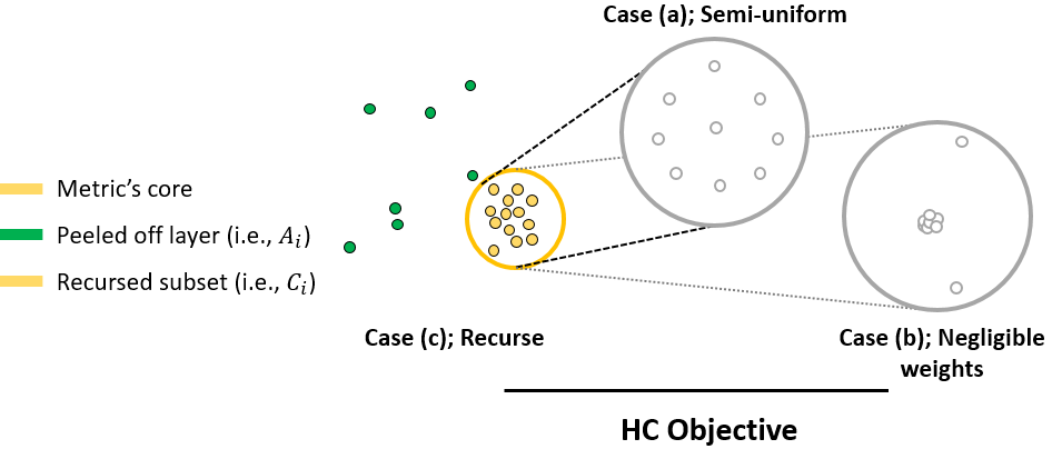
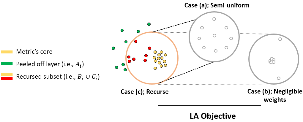
Figure 1: A recursion step (case (c)) and the two possible halting steps (cases (a) and (b)). The yellow points define the metric’s core. In the HC case we peel off both red and green points in a single step, while in the LA we must be more delicate and only peel off the green points.

Before defining our algorithms we need the following definitions.

Definition 2.1.

Let $G=(V,w)$ denote a metric and $U\subset V$ denote a subset of its nodes. We introduce the following notations: (1) let $\mathbf{D_{U}}=\max_{i,j\in U}w_{i,j}$ denote $U$’s diameter, (2) let $\mathbf{W_{U}}=\sum_{i,j\in U}w_{i,j}$ denote $U$’s sum of weights, (3) let $\mathbf{n_{U}}=|U|$ denote $U$’s size and (4) let $\mathbf{\rho_{U}}=\frac{W_{U}}{n_{U}^{2}D_{U}}$ denote $U$’s weighted density.

All our algorithms will make use of the following simple yet useful structural lemma that states that for small-density instances there exists a large cluster of nodes with a small diameter. The proof is deferred to the Appendix.

Lemma 2.2.

For any metric $G=(V,w)$ there exists a set $U\subset V$ such that $D_{U}\leq 4D_{V}\sqrt{\rho_{V}}$ and $n_{U}\geq n_{V}(1-\sqrt{\rho_{V}})$.

Definition 2.3.

Given a metric $G=(V,w)$ we denote $U\subset V$ as guaranteed by Lemma 2.2 as a metric’s core.

Note that the core can be found algorithmicaly simply through brute force (while the core need not be unique, our algorithms will choose one arbitrarily).

Throughout our paper we consider different metric-based objectives. In order to solve them, we apply the same recipe - if the instance is sufficiently densely weighted, apply an algorithm for these types of instances. Otherwise, the algorithm detects the metric’s core (which is a small-diameter subset containing almost all nodes) and peel off (and subsequently embed) a layer of data points that are far from the core. The algorithm then considers the core; if it is sufficiently small (in terms of inner weights) then we embed the core arbitrarily and halt. Otherwise, we recurse on the core. Our algorithms for both objectives (LA and HC) will follow the same structure as defined in Algorithm 1.

if the instance is sufficiently densely weighted then // case (a)

       Solve it using $ALG_{d-w}$.

else

       Let $C$ denote the metric’s core (as defined by Definition 2.3).

      Define the layer to peel off $A\subset V\setminus C$ appropriately.

      Embed $A$.

      if $W_{V\setminus A}$ is negligible then  Embed $V\setminus A$ arbitrarily and return.

        // case (b) else  Continue recursively on $V\setminus A$

        // case (c)

Algorithm 1 General Algorithm

We denote by cases (a) and (b) the different cases for which the algorithm may terminate and by case (c) the recursive step. We further denote by $ALG_{d-w}$ an auxiliary algorithm that will handle sufficiently densely weighted instances. (These algorithms will differ according to the different objectives).

Henceforth, given an algorithm $ALG$ and metric $G$ we denote by $ALG(G)$ the algorithm’s returned embedding. We note that when clear from context we overload the notation and denote $ALG(G)$ as the embedding’s value under the respective objectives. Equivalently, we will use the term $OPT(G)$ for the optimal embedding.

Our different algorithms will be similarly defined and thus so will their analyses. Thus, we introduce a general scheme for analyzing such algorithms. Let $k$ denote the number of recursive calls our algorithm performs. Furthermore, let $G_{i}$ denote the instance the algorithm is called upon in step $i$ for $i=0,1,\ldots,k$. (I.e., $G=G_{0}$ and $ALG(G_{k})$ does not perform a recursive step, meaning that it terminates with case (a) or (b)). We first observe that by applying a simple averaging argument we get the following useful observation.

Observation 2.4.

If there exist $\alpha_{i},\beta_{i},\gamma_{i}>0$ such that $ALG(G_{i})\geq\alpha_{i}+ALG(G_{i+1})$ and $OPT(G_{i})\leq\beta_{i}+\gamma_{i}OPT(G_{i+1})$ for all $i=0,\ldots,k-1$ then

$$\frac{ALG(G)}{OPT(G)}\geq\frac{\sum_{i=0}^{k-1}\alpha_{i}+ALG(G_{k})}{\sum_{i=0}^{k-1}\big{(}\beta_{i}\Pi_{j=0}^{i-1}\gamma_{j}\big{)}+(\Pi_{i=0}^{k-1}\gamma_{i})OPT(G_{k})}\geq\min\{\min_{i}\{\frac{\alpha_{i}}{\beta_{i}\Pi_{j=0}^{i-1}\gamma_{j}}\},\frac{ALG(G_{k})}{(\Pi_{i=0}^{k-1}\gamma_{i})OPT(G_{k})}\}.$$

Thus, in order to analyze a given algorithm, it will be enough to set the values of $\alpha_{i}$, $\beta_{i}$ and $\gamma_{i}$, and further analyze the approximation ratio of $\frac{ALG(G_{k})}{OPT(G_{k})}$ for the different terminating cases (cases (a) and (b)).

3 Notations and Preliminaries

We introduce the following notation to ease our presentation later on.

Definition 3.1.

Given a metric $G=(V,w)$, a solution $\mathbf{SOL(G)}$ for the LA objective and disjoints sets $A,B\subset V$ we define: $\mathbf{\left.SOL(G)\right|_{A}}=\sum_{i,j\in A}w_{i,j}y_{i,j}$ and $\mathbf{\left.SOL(G)\right|_{A,B}}=\sum_{i\in A,j\in B}w_{i,j}y_{i,j}$. For the HC objective the notations are defined symmetrically by replacing $y_{i,j}$ with $|T_{i,j}|$.

We will make use of algorithms belonging to the following class of algorithms.

Definition 3.2.

An algorithm is considered an Efficient Polytime Randomized Approximation Scheme (EPRAS) if for any $\epsilon>0$ the algorithm has expected running time of $f(\frac{1}{\epsilon})n^{O(1)}$ and approximates the optimal solution’s value up to a factor of $1-\epsilon$.

We will frequently use the following (simple) observations and thus we state them here.

Observation 3.3.

Given values $\alpha_{i}\geq 0$, $\alpha\in(0,\frac{1}{k(k+1)})$ and $k\in\mathbb{N}$ we have: (1) $\Pi_{i}(1-\alpha_{i})\geq 1-\sum_{i}\alpha_{i}$, (2) $1+k\alpha<\frac{1}{1-k\alpha}<1+(k+1)\alpha$ and (3) $1+k\alpha<e^{k\alpha}<1+(k+1)\alpha$.

The following facts will prove useful in our subsequent proofs and are therefore stated here.

Fact 3.4.

Given a metric $G$, if the optimal linear arrangement under the LA objective is $OPT_{LA}(G)$ and the optimal hierarchical clustering under the HC objective is $OPT_{HC}(G)$ then we have $OPT_{LA}(G)\geq\frac{1}{3}n\sum_{i,j}w_{i,j}y_{i,j}$ and $OPT_{HC}(G)\geq\frac{2}{3}n\sum_{i,j}w_{i,j}|T_{i,j}|$.

We note that the HC portion of Fact 3.4 has been used widely in the literature (e.g., see proof in Cohen-Addad et al. (2018)). The LA portion of Fact 3.4 is mentioned in Hassin and Rubinstein Hassin and Rubinstein (2001). Finally, in the HC section we make use of ”ladder” HC trees. We define them here.

Definition 3.5.

We define a ”ladder” as an HC tree that cuts a single data point from the rest at every cut (or internal node).

4 The Linear Arrangement Objective

We will outline the section as follows. We begin by presenting our algorithms (first the algorithm that handles case (a) and thereafter the general algorithm). We will then bound the algorithm’s approximation guarantee (by following the bounding scheme of Observation 2.4). Finally, we will analyze the algorithm’s running time.

4.1 Defining the Algorithms

Here we begin by applying our general algorithm to the linear arrangement problem (which we will denote simply as $ALG$). The algorithm uses, as a subroutine, an algorithm to handle case (a). We denote this subroutine as $ALG_{d-w}$ and define it following the definition of $ALG$.

4.1.1 Defining $ALG$

Here we apply our general algorithm (Algorithm 1) to the linear arrangement setting. In order to do so, roughly speaking, we define the layer to peel off $A$ as the set of all points which are ”far” from the metric’s core. We also introduce a subroutine to handle densely weighted instances, $ALG_{d-w}$.

if $\rho\geq\epsilon^{6}$ then  solve it using $ALG_{d-w}$.

  // case (a) else

       Let $C$ denote the metric’s core (as defined by Lemma 2.2).

      Let $A$ denote all data points that are of distance $\geq\epsilon^{2}D_{V}$ from $C$.

      Place $A$ to the left of $V\setminus A$. Arrange $A$ arbitrarily.

      if $W_{V\setminus A}<\epsilon W_{V}$ then  Arrange $V\setminus A$ arbitrarily and return.

        // case (b) else  Continue recursively on $V\setminus A$.

        // case (c)

Algorithm 2 Linear Arrangement Algorithm ($ALG$)

The set $V\setminus\{A\cup C\}$ will be used frequently in the upcoming proofs and thus we give it its own notation.

Definition 4.1.

Denote $B=V\setminus\{A\cup C\}$ where $A$ and $C$ are defined as in Algorithm 2.

4.1.2 Defining $ALG_{d-w}$

Here we will introduce an algorithm to handle case (a) type instances. Before formally defining the algorithm, we will first provide some intuition. Towards that end we first introduce the following definition.

Definition 4.2.

Consider $OPT(G_{k})$’s embedding into the line, $[n]$. Partition $[n]$ into $\frac{1}{\epsilon}$ consecutive sets each of size $\epsilon n$ and let $P_{i}^{*}$ denote the points embedded by $OPT(G_{k})$ into the $i$’th consecutive set. Furthermore, denote by $P^{*}=\{P_{i}^{*}\}$ the induced partition of the metric.

Later on, we will show that $OPT(G_{k})$’s objective value is closely approximated by the value generated solely from inter-partition-set edges (i.e., any $(u,v)$ where $u,v$ lie in different partition sets of $P^{*}$). While $OPT(G_{k})$ cannot be found algorithmically, assuming the above holds, it is enough for $ALG_{d-w}$ to guess the partition $P^{*}$. Indeed, that is exactly what we will do, by using the general graph partitioning algorithm of Goldreich et al. Goldreich et al. (1998).

We denote the General Graph Partitioning algorithm of Goldreich et al. Goldreich et al. (1998) as $PT(G,\Phi,\epsilon_{err})$. See Definition 4.10 for a definition of $\Phi$ and $\epsilon_{err}$ (these will be defined by $ALG_{d-w}$ as well) and see Theorem 4.11 for the tester’s guarantees. We are now ready to define our algorithm that handles sufficiently densely weighted instances (Algorithm 3).

Let $k=\frac{1}{\epsilon}$ denote the size of the partition.

for $\{\mu_{j,j^{\prime}}\}_{j\leq k,j^{\prime}\leq k,j\neq j^{\prime}}\subset\{i\epsilon^{9}n^{2}D_{V}:i\in\mathbb{N}\land i\leq\frac{1}{\epsilon^{7}}\}$ do

       Let $\Phi=\{\epsilon n,\epsilon n\}_{j=1}^{k}\cup\{\mu_{j,j^{\prime}},\mu_{j,j^{\prime}}\}_{j,j^{\prime}=1}^{k}$.

      Run $PT(G,\Phi,\epsilon_{err}=\epsilon^{9})$. Let $P$ denote the output partition (if succeeded).

      Let $\widehat{y}$ denote the linear arrangement obtained from embedding $P$ consecutively on the line (and arbitrarily within the partition sets).

      Compute the value $\sum_{e}w_{e}\widehat{y_{e}}$ for $P$.

Return the partition with maximum $\sum_{e}w_{e}\widehat{y_{e}}$ value.

Algorithm 3 LA Algorithm for Sufficiently Densely Weighted Instances ($ALG_{d-w}$)

4.2 Analyzing the Approximation Ratio of $ALG$

Now that we have defined $ALG$ we are ready to analyze its approximation ratio. Recall that by Observation 2.4 it is enough to analyze the approximation ratio of cases (a), (b) and the total loss incurred by the recursion steps (i.e., by setting $\alpha_{i}$, $\beta_{i}$ and $\gamma_{i}$).

4.2.1 Structural Lemmas

Recall that we defined $k$ to be the number of recursion steps used by $ALG$ and that $G_{i}$ is the instance that $ALG$ is applied to at recursion step $i$. Further recall that given $G_{i}$, $ALG(G_{i})$ partitioned the instance into $A_{i},B_{i}$ and $C_{i}$ and that, informally, by Lemma 2.2 $n_{C_{i}}$ contains the majority of the data points and $D_{C_{i}}$ is relatively small compared to $D_{V_{i}}$.

By the definition of $C_{i}$, $A_{i}$ could be considered as a set of outliers. Therefore, intuitively it makes sense to split $A_{i}$ from $C_{i}$. In order to prove our algorithm’s approximation ratio we will show that in fact one does not lose too much compared to optimal solution, by splitting $A_{i}$ from $C_{i}$. In order to do so we will show that in fact, both the values of $ALG$ and $OPT$ will be roughly equal to $\frac{1}{2}nW_{A_{i},C_{i}}$ (which makes sense intuitively since $C_{i}$ is of low diameter and contains many points and $A_{i}$ are the points that are far from this cluster).

The following lemmas consider 2 types of algorithms - algorithms that split $A_{i}$ and $C_{i}$ and algorithms that do not. Furthermore, they show that in fact, by the structural properties of $A_{i}$ and $C_{i}$, if we consider the values generated by these 2 types of algorithms restricted to the objective value generated by the inter-weights $W_{A_{i},C_{i}}$, are approximately equal. We begin by lower bounding the value generated by algorithms that split $A_{i}$ and $C_{i}$. Due to lack of space, we defer the following proofs to the Appendix.

Lemma 4.3.

Given the two disjoint sets $C_{i}$ and $A_{i}$ and a linear arrangement $y$ that places all nodes in $A_{i}$ to the left of all nodes in $C_{i}$ we are guaranteed that

$$\sum_{c\in C_{i},a\in A_{i}}w_{a,c}y_{a,c}\geq\frac{n_{C_{i}}}{2}(W_{C_{i},A_{i}}-n_{C_{i}}n_{A_{i}}D_{C_{i}}).$$

Due to the fact that $C_{i}$ is a small cluster containing most of the data points the above lemma reduces to the following corollary.

Corollary 4.4.

Given any linear arrangement $y$ that places all nodes in $A_{i}$ to the left of all nodes in $C_{i}$ we are guaranteed that

$$\sum_{a\in A_{i},c\in C_{i}}w_{a,c}y_{a,c}\geq\frac{1}{2}nW_{A_{i},C_{i}}(1-\frac{5\sqrt{\rho}}{\epsilon^{2}})$$

Now that we have lower bounded algorithms that split $A_{i}$ and $C_{i}$ we will upper bound algorithms that do not have this restriction. (Note that we begin by handling the case where one of the disjoint sets is a single data point and thereafter generalize it to two disjoint sets).

Lemma 4.5.

Given a set $C_{i}$ and a point $p\not\in C_{i}$, we are guaranteed that

$$\begin{gathered}\sum_{c\in C_{i}}w_{p,c}y_{p,c}\leq(W_{p,C_{i}}+n_{C_{i}}D_{C_{i}})(n-\frac{n_{C_{i}}}{2}).\end{gathered}$$

We are now ready to upper bound the inter-objective-value of two sets of disjoint points.

Lemma 4.6.

Given the two disjoint sets $C_{i}$ and ${A_{i}}$ and any linear arrangement $y$ we are guaranteed that

$$\sum_{c\in C_{i},a\in{A_{i}}}w_{a,c}y_{a,c}\leq(n-\frac{n_{C_{i}}}{2})(W_{C_{i},{A_{i}}}+n_{C_{i}}n_{A_{i}}D_{C_{i}}).$$

Due to the fact that $C_{i}$ is a small cluster containing most of the data points the lemma reduces to the following corollary.

Corollary 4.7.

Given any linear arrangement $y$ we are guaranteed that

$$\sum_{a\in A_{i},c\in C_{i}}w_{a,c}y_{a,c}\leq\frac{1}{2}nW_{A_{i},C_{i}}(1+\frac{9\sqrt{\rho}}{\epsilon^{2}}).$$

We will want to show that the objective values of both $ALG$ and $OPT$ (and some other intermediate values that will be defined later on) are approximately determined by their value on the inter-weights of $W_{A_{i},C_{i}}$. In order to do so, we first introduce the following structural lemma that will help us explain this behaviour.

Lemma 4.8.

Given an instance $G$ and sets $A,B$ and $C$ as defined by $ALG(G)$ we have $W_{A}+W_{A,B}\leq 2\frac{\sqrt{\rho}}{\epsilon^{2}}W_{A,C}.$

4.2.2 Analyzing the Approximation Ratio of Case (a) of $ALG$

We first give an overview the approximation ratio analysis. Recall the definition of $P^{*}$ (Definition 4.2). The first step towards our proof, is to show that instead of trying to approximate $OPT(G_{k})$, it will be enough to consider its value restricted to intra-partition-set weights with respect to $P^{*}$. Even more, for such weights $w_{u,v}$, incident to $P^{*}_{i}$ and $P^{*}_{i+j}$, it will be enough to assume that their generated value towards the objective (i.e., the value $y_{u,v}$) is only $(j-1)\epsilon n$ (while it may be as large as $(j+1)\epsilon n$). Formally, this will be done in Lemma 4.9 (whose proof is deferred to the Appendix).

Next, recall that $ALG_{d-w}$ tries to guess the partition $P^{*}$ (up to some additive error) and let $P$ denote the partition guessed by $ALG_{d-w}$. Observe that if guessed correctly, the value generated towards $ALG$’s objective for any intra-partition-set weight crossing between $P_{i}$ and $P_{i+j}$ is at least $|P_{i+1}|+\cdots|P_{i+j-1}|$ and if we managed to guess the set sizes as well then this value is exactly $(j-1)\epsilon n$ (equivalent to that of $OPT$’s). This will be done in Proposition 4.12.

Lemma 4.9.

Given the balanced line partition of set sizes $\epsilon n$, denoted as $P^{*}$, we have

$$OPT(G_{k})\leq(1+13\epsilon)\sum_{\begin{subarray}{c}1\leq i\leq k-1\\ 1\leq j\leq k-i\end{subarray}}W_{P^{*}_{i},P^{*}_{i+j}}(|P^{*}_{i+1}|+\cdots+|P^{*}_{i+j-1}|).$$

Before proving Proposition 4.12 we state the properties of the general graph partitioning algorithm of Goldreich et al. Goldreich et al. (1998).

Definition 4.10 (Goldreich et al. (1998)).

Let $\Phi=\{\lambda_{j}^{LB},\lambda_{j}^{UB}\}_{j=1}^{k}\cup\{\mu_{j,j^{\prime}}^{LB},\mu_{j,j^{\prime}}^{UB}\}_{j,j^{\prime}=1}^{k}$ denote a set of non-negative values such that $\lambda_{j}^{LB}\leq\lambda_{j}^{UB}$ and $\mu_{j,j^{\prime}}^{LB}\leq\mu_{j,j^{\prime}}^{UB}$. We define $\mathcal{GP}_{\Phi}$ the set of graphs $G$ on $n$ vertices that have a $k$ partition $(V_{1},\ldots,V_{k})$ upholding the following constraints

$$\begin{gathered}\forall j:\,\lambda_{j}^{LB}\leq\frac{|V_{j}|}{n}\leq\lambda_{j}^{UB};\quad\forall j,j^{\prime}:\,\mu_{j,j^{\prime}}^{LB}\leq\frac{W_{V_{j},V_{j^{\prime}}}}{n^{2}}\leq\mu_{j,j^{\prime}}^{UB}.\end{gathered}$$

Theorem 4.11 (Goldreich et al. (1998)).

Given inputs $G=(V,w)$ with $|V|=n$ and $w:V\times V\rightarrow[0,1]$ describing the graph and $\Phi$ describing bounds on the wanted partition, $\epsilon_{err}$, the algorithm $PT(G,\Phi,\epsilon_{err})$ has expected running time of

$$\exp\big{(}\log(\frac{1}{\epsilon_{err}})\cdot(\frac{O(1)}{\epsilon_{err}})^{k+1}\big{)}+O(\frac{\log{\frac{k}{\epsilon_{err}}}}{\epsilon_{err}^{2}})\cdot n.$$

Furthermore, if $G\in\mathcal{GP}_{\Phi}$ as in Definition 4.10 then the algorithm outputs a partition satisfying

• $\forall j:\,\,\lambda_{j}^{LB}-\epsilon_{err}\leq\frac{|V_{j}|}{n}\leq\lambda_{j}^{UB}+\epsilon_{err}$,

• $\forall j,j^{\prime}:\,\,\mu_{j,j^{\prime}}^{LB}-\epsilon_{err}\leq\frac{W_{V_{j},V_{j^{\prime}}}}{n^{2}}\leq\mu_{j,j^{\prime}}^{UB}+\epsilon_{err}$.

We are now ready to prove Proposition 4.12.

Proposition 4.12.

If $ALG$ terminates in case (a) then $\frac{ALG_{d-w}(G_{k})}{OPT(G_{k})}=\frac{ALG(G_{k})}{OPT(G_{k})}\geq 1-20\epsilon.$

Proof.

Let $P=\{P_{i}\}$ denote the partition returned by $PT(G_{k},\Phi,\epsilon_{err})$ and recall that its number of sets is $k=\frac{1}{\epsilon}$ and that $\epsilon_{err}=\epsilon^{9}$. We first observe that by Theorem 4.11 we are guaranteed that the error in $|P_{i}|$ compared to $|P^{*}_{i}|=\epsilon n$ is at most $|P_{i}|\geq\epsilon n-\epsilon_{err}n$ (due to the fact that in $\Phi$ we requested sets of size exactly $\epsilon n$). Therefore

$$\begin{gathered}ALG_{d-w}\geq\sum_{\begin{subarray}{c}1\leq i\leq k-1\\ 1\leq j\leq k-i\end{subarray}}W_{P_{i},P_{i+j}}(|P_{i+1}|+\cdots+|P_{i+j-1}|)\geq\sum_{\begin{subarray}{c}1\leq i\leq k-1\\ 1\leq j\leq k-i\end{subarray}}(j-1)(\epsilon n-\epsilon_{err}n)W_{P_{i},P_{i+j}},\end{gathered}$$ (1)

where $W_{P_{i},P_{i+j}}$ denotes the weight crossing between $P_{i}$ and $P_{i+j}$. For ease of presentation we will remove the subscript in the summation henceforth.

Consider the difference between the cut size of $W_{P_{i},P_{i+j}}$ and $W_{P^{*}_{i},P^{*}_{i+j}}$. Their difference originates from two errors: (1) the error that incurred by the PT algorithm (see Theorem 4.11) and (2) the error $ALG_{d-w}$ incurred in order to guess the partition of $OPT(G_{k})$ (see Algorithm 3). Therefore,

$$W_{P_{i},P_{i+j}}\geq W_{P^{*}_{i},P^{*}_{i+j}}-\epsilon_{err}n^{2}D_{V}-\epsilon^{9}n^{2}D_{V}=W_{P^{*}_{i},P^{*}_{i+j}}-2\epsilon^{9}n^{2}D_{V}$$

where the last equality is since $\epsilon_{err}=\epsilon^{9}$. Combining this with inequality 1 yields

$$\begin{gathered}ALG_{d-w}\geq(\epsilon n-\epsilon_{err}n)\cdot\sum(j-1)W_{P^{*}_{i},P^{*}_{i+j}}-(\epsilon n-\epsilon_{err}n)\cdot 2(\epsilon^{9}n^{2})D_{V}\sum(j-1)\geq\\ (\epsilon n-\epsilon_{err}n)\cdot\sum(j-1)W_{P^{*}_{i},P^{*}_{i+j}}-2n^{3}\epsilon^{7}D_{V},\end{gathered}$$ (2)

where the last inequality follows since $\epsilon_{err}>0$ and $\sum(j-1)=\sum_{i=1}^{k}\sum_{j=i+1}^{k}(j-1)\leq k^{3}=\epsilon^{-3}$.

Due to the fact that we are in case (a) we have that $\frac{W}{n^{2}D_{V}}=\rho\geq\epsilon^{6}$. By Fact 3.4 we have that $OPT\geq\frac{1}{3}nW$ and therefore $2n^{3}\epsilon^{7}D_{V}$ can be bounded by $2n^{3}\epsilon^{7}D_{V}\leq 2\epsilon nW\leq 6\epsilon OPT$. Thus we get $2n^{3}\epsilon^{7}D_{V}\leq 6\epsilon OPT(G_{k})$. Combining this with inequality 2 yields

$$ALG_{d-w}\geq(\epsilon n-\epsilon_{err}n)\cdot\sum(j-1)W_{P^{*}_{i},P^{*}_{i+j}}-6\epsilon OPT(G_{k}).$$ (3)

On the other hand, recall that $P^{*}$ denotes the balanced partition where all sets are of size $\epsilon n$. Therefore, by Lemma 4.9 we therefore get

$$\begin{gathered}OPT(G_{k})\leq(1+13\epsilon)\sum W_{P^{*}_{i},P^{*}_{i+j}}(|P^{*}_{i+1}|+\cdots+|P^{*}_{i+j-1}|)=\\ (1+13\epsilon)\sum(j-1)(\epsilon n)W_{P^{*}_{i},P^{*}_{i+j}}=\epsilon n(1+13\epsilon)\cdot\sum(j-1)W_{P^{*}_{i},P^{*}_{i+j}}.\end{gathered}$$ (4)

Combining inequalities 3 and 4 yields

$$\begin{gathered}ALG_{d-w}\geq\frac{\epsilon n-\epsilon_{err}n}{\epsilon n(1+13\epsilon)}OPT(G_{k})-6\epsilon OPT(G_{k})=\\ \frac{1-\epsilon^{8}}{1+13\epsilon}OPT(G_{k})-6\epsilon OPT(G_{k})\geq(1-20\epsilon)OPT(G_{k}),\end{gathered}$$

thereby concluding the proof. ∎

4.2.3 Analyzing the Approximation Ratio of Case (b) of $ALG$

Using our structural lemmas we will analyze the approximation ratio of $ALG$ applied to $G_{k}$ under the assumption that the algorithm terminated in case (b) (i.e., that $\rho<\epsilon^{6}$ and $W_{B\cup C}\leq\epsilon W_{G_{k}}$). The full proof is deferred to the Appendix.

Proposition 4.13.

If $ALG$ terminates in case (b) then $\frac{ALG(G_{k})}{OPT(G_{k})}\geq 1-33\epsilon.$

Sketch.

The proof follows the following path. Due to the fact that most of the instance’s density is centered at the metric’s core $C$, the majority of $OPT(G_{k})$’s objective is derived from weights incident to $C$. Since we are case (b), the weight of $W_{B\cup C}$ is negligible and therefore we will show that in fact $OPT(G_{k})$’s objective is defined by $\left.OPT(G_{k})\right|_{A,C}$. Thereafter, we show that in fact the best strategy to optimize for weights in $W_{A,C}$ is to place $A$ at one extreme of the line and $C$ at the other - which, fortunately, is what $ALG(G_{k})$ (approximately) does - thereby approximating $OPT(G_{k})$. ∎

4.2.4 Setting the Values $\alpha_{i}$, $\beta_{i}$ and $\gamma_{i}$

Due to lack of space, the following proofs are deferred to the Appendix.

Proposition 4.14.

For $A_{i}$ and $C_{i}$ as defined by our algorithm applied to $G_{i}$ and for $\alpha_{i}=\frac{1}{2}nW_{A,C}(1-\frac{5\sqrt{\rho}}{\epsilon^{2}})$, we have $ALG(G_{i})\geq\alpha_{i}+ALG(G_{i+1})$.

Proposition 4.15.

Let $G_{i}=(V_{i},w_{i})$ and $G_{i+1}=(V_{i+1},w_{i+1})$ denote the instances defined by the $i$ and $i+1$ recursion steps. Furthermore let $\beta_{i}=\frac{1}{2}n_{V_{i}}W_{A_{i},C_{i}}(1+\frac{13\sqrt{\rho}}{\epsilon^{2}})$ and $\gamma_{i}=1+4\sqrt{\rho_{i}}$. Therefore, $OPT(G_{i})\leq\beta_{i}+\gamma_{i}OPT(G_{i+1}).$

Thus, we have managed to set the values of $\alpha_{i}$, $\beta_{i}$ and $\gamma_{i}$ as follows.

Definition 4.16.

We define the values $\alpha_{i}$, $\beta_{i}$ and $\gamma_{i}$ as follows

$$\begin{gathered}\alpha_{i}=\frac{1}{2}nW_{A_{i},C_{i}}(1-\frac{5\sqrt{\rho_{i}}}{\epsilon^{2}});\quad\beta_{i}=\frac{1}{2}n_{V_{i}}W_{A_{i},C_{i}}(1+\frac{13\sqrt{\rho_{i}}}{\epsilon^{2}});\quad\gamma_{i}=1+4\sqrt{\rho_{i}}.\end{gathered}$$ (5)

4.2.5 Putting it all Together

Now that we have analyzed the terminal cases of the algorithm (cases (a) and (b)) and that we have set the values of $\alpha_{i}$, $\beta_{i}$ and $\gamma_{i}$ we will to combine these results to prove $ALG$’s approximation ratio (as in Observation 3.3). In order to so we must therefore bound the values $\min_{i}\{\frac{\alpha_{i}}{\beta_{i}\Pi_{j=0}^{i-1}\gamma_{j}}\}$ and $\frac{ALG(G_{k})}{(\Pi_{i=0}^{k-1}\gamma_{i})OPT(G_{k})}$. However, before doing so we will first show that $\Pi_{j=0}^{i-1}\gamma_{j}$ converges. Recall that $\gamma_{i}=1+4\sqrt{\rho_{i}}$. The following lemma shows that the instances’ densities ($\rho_{i}$) increase at a fast enough rate (exponentially) in order for $\Pi_{j=0}^{i-1}\gamma_{j}$ to converge.

Lemma 4.17.

For all $i=1,\ldots,k-1$ we are guaranteed that $\rho_{i+1}\geq 4\rho_{i}$.

Proof.

Let $V$ denote the set of nodes of $G_{i}$. Recall the notations $A$, $B$ and $C$ defined by our algorithm applied to $V$ (in particular, the set of nodes of $G_{i+1}$ is exactly $B\cup C$). Therefore, if we denote by $D_{B-C}$ the largest distance between any point in $B$ and its closest point in $C$, then $D_{B\cup C}\leq 2D_{B-C}+D_{C}\leq 2\epsilon^{2}D_{V}+4D_{V}\sqrt{\rho_{i}},$ where the first inequality follow from the triangle inequality and the second follows due to the fact that $B$ is defined as the set of all points of distance at most $\epsilon^{2}$ from $C$. Therefore,

$$\begin{gathered}\rho_{i+1}=\frac{W_{B\cup C}}{n^{2}_{B\cup C}\cdot D_{B\cup C}}\geq\frac{W_{V}}{n^{2}_{V}\cdot D_{V}}(\frac{\epsilon}{2\epsilon^{2}+4\sqrt{\rho_{i}}})=\rho_{i}(\frac{\epsilon}{2\epsilon^{2}+4\sqrt{\rho_{i}}}),\end{gathered}$$ (6)

where the equalities follows by the definition of $\rho_{i}$ and the inequality follows due to the fact that $W_{B\cup C}\geq\epsilon W_{V}$ (which follows due to the fact that we are in case (c)), $n_{B\cup C}\leq n_{V}$ and $D_{B\cup C}\leq(2\epsilon^{2}+4\sqrt{\rho_{i}})D_{V}$ (as stated above). Since we are in case (c), we are guaranteed that $\rho_{i}\leq\epsilon^{6}$ and therefore

$$\begin{gathered}\frac{\epsilon}{2\epsilon^{2}+4\sqrt{\rho_{i}}}\geq\frac{\epsilon}{2\epsilon^{2}+4\epsilon^{3}}\geq\frac{1}{3\epsilon},\end{gathered}$$ (7)

since $\epsilon\leq 10^{-2}$. Combining inequalities 6 and 7, and since $\epsilon<10^{-2}$ yields $\rho_{i+1}\geq\rho_{i}(\frac{\epsilon}{2\epsilon^{2}+4\sqrt{\rho_{i}}})\geq\frac{\rho_{i}}{3\epsilon}\geq 4\rho_{i},$ thereby concluding the proof. ∎

We are now ready to show that $\Pi_{j=0}^{i-1}\gamma_{j}$ converges.

Lemma 4.18.

For $\gamma_{i}=1+4\sqrt{\rho_{i}}$ we have $\Pi_{j=0}^{i-1}\gamma_{j}\leq 1+5\sqrt{\rho_{i}}$.

Proof.

Observe that $\Pi_{j=0}^{i-1}(1+4\sqrt{\rho_{j}})\leq e^{4\cdot\sum_{j}\sqrt{\rho_{j}}}\leq e^{4\sqrt{\rho_{i}}}\leq 1+5\sqrt{\rho_{i}},$ where the first inequality follows from Observation 3.3, the second follows since $\sqrt{\rho_{j}}$ are exponentially increasing (Lemma C.1) and the third inequality follows again by Observation 3.3 combined with the fact that $\rho<\epsilon^{2}$ and $\epsilon<10^{-2}$. ∎

Next we leverage the former lemma to bound $\min_{i}\{\frac{\alpha_{i}}{\beta_{i}\Pi_{j=0}^{i-1}\gamma_{j}}\}$ and $\frac{ALG(G_{k})}{(\Pi_{i=0}^{k-1}\gamma_{i})OPT(G_{k})}$.

Proposition 4.19.

For $\alpha_{i}$, $\beta_{i}$ and $\gamma_{i}$ as in Definition 4.16, we have $\min_{i}\{\frac{\alpha_{i}}{\beta_{i}\Pi_{j=0}^{i-1}\gamma_{j}}\}\geq 1-23\epsilon$.

Proof.

We first bound $\frac{\alpha_{i}}{\beta_{i}}$. By the definitions of $\alpha_{i}$ and $\beta_{i}$ we have

$$\begin{gathered}\frac{\alpha_{i}}{\beta_{i}}=\frac{1-\frac{5\sqrt{\rho_{i}}}{\epsilon^{2}}}{1+\frac{13\sqrt{\rho_{i}}}{\epsilon^{2}}}\geq(1-\frac{5\sqrt{\rho_{i}}}{\epsilon^{2}})(1-\frac{13\sqrt{\rho_{i}}}{\epsilon^{2}})\geq 1-\frac{18\sqrt{\rho_{i}}}{\epsilon^{2}},\end{gathered}$$ (8)

where the first inequality follows from the definitions of $\alpha_{i}$ and $\beta_{i}$ and the rest of the inequalities follow since $\epsilon<10^{2}$ and $\rho<\epsilon^{6}$.

By Lemma 4.18 we are guaranteed that $\Pi_{j=0}^{i-1}\gamma_{j}\leq 1+5\sqrt{\rho_{i}}$. Combining this with inequality 8 yields

$$\frac{\alpha_{i}}{\beta_{i}\Pi_{j=0}^{i-1}\gamma_{j}}\geq\frac{1-\frac{18\sqrt{\rho_{i}}}{\epsilon^{2}}}{1+5\sqrt{\rho_{i}}}\geq(1-\frac{18}{\epsilon^{2}}\sqrt{\rho_{i}})(1-5\sqrt{\rho_{i}})\geq 1-\frac{23}{\epsilon^{2}}\sqrt{\rho_{i}},$$

and since $\rho_{i}$ only increases and $\rho_{k-1}\leq\epsilon^{6}$ we have $\min_{i}\{\frac{\alpha_{i}}{\beta_{i}\Pi_{j=0}^{i-1}\gamma_{j}}\}\geq 1-\frac{23}{\epsilon^{2}}\sqrt{\rho_{k-1}}\geq 1-23\epsilon$, thereby concluding the proof. ∎

Proposition 4.20.

For $\gamma_{i}=1+4\sqrt{\rho_{i}}$ we have $\frac{ALG(G_{k})}{(\Pi_{i=0}^{k-1}\gamma_{i})OPT(G_{k})}\geq 1-34\epsilon$.

Proof.

By Propositions 4.12 and 4.13 we are guaranteed that $\frac{ALG(G_{k})}{OPT(G_{k})}\geq 1-33\epsilon$. On the other hand by by Lemma 4.18 we are guaranteed that $\Pi_{i=0}^{k-2}\gamma_{i}\leq 1+5\sqrt{\rho_{k-1}}$. Therefore, if $k=1$ then $\frac{ALG(G_{k})}{(\Pi_{i=0}^{k-1}\gamma_{i})OPT(G_{k})}=\frac{ALG(G_{k})}{OPT(G_{k})}\geq 1-33\epsilon.$ Otherwise, we have

$$\frac{ALG(G_{k})}{(\Pi_{i=0}^{k-1}\gamma_{i})OPT(G_{k})}\geq\frac{1-33\epsilon}{(1+4\sqrt{\rho_{k-1}})(1+5\sqrt{\rho_{k-1}})}\geq\frac{1-33\epsilon}{(1+4\epsilon^{3})(1+5\epsilon^{3})}\geq 1-34\epsilon,$$

where the second inequality follows since $\rho_{k-1}<\epsilon^{6}$ (since we recursed to step $k$) and the subsequent inequalities follow since $\epsilon<10^{-3}$ - thereby concluding the proof. ∎

Finally, we combine Propositions 4.19 and 4.20 to bound $ALG$’s approximation ratio.

Theorem 4.21.

For any metric $G$, $\frac{ALG(G)}{OPT(G)}\geq 1-34\epsilon$.

4.3 Analyzing the Running Time of $ALG$

Consider the definition of $ALG$. We observe that in each recursion step, the algorithm finds the layer to peel off, $A$, and then recurses. Therefore the running time is defined by the sum of these recursion steps, plus the terminating cases (i.e., either case (a) or case (b)). Recall that case (a) applies $ALG_{d-w}$ on the instance, while case (b) arranges the instance arbitrarily. Therefore, a bound on cases (a) and (b) is simply a bound on the running time of $ALG_{d-w}$ which is given by Lemma 4.22 (whose proof appears in the Appendix).

Lemma 4.22.

Given an instance $G$, the running time of $ALG_{d-w}(G)$ is at most $(\frac{1}{\epsilon^{7}})^{\frac{1}{\epsilon^{2}}}\cdot O(n^{2})$.

Remark 4.23.

A bi-product of Lemma 4.17 is that the number of recursion steps is bounded by $O(\log n)$. The proof follows similarly to the proof of Lemma C.3 substituting the inequality $\rho_{i+1}\geq 4\epsilon\sqrt{\rho_{i}}$ with $\rho_{i+1}\geq 4\sqrt{\rho_{i}}$ (which holds due to Lemma 4.17).

We are now ready to analyze the running time of $ALG$. (The proof is deferred to the Appendix.)

Theorem 4.24.

The algorithm $ALG$ is an EPRAS (with running time $O(n^{2}\log n)$ plus the running time of $ALG_{d-w}$).

Remark 4.25.

We remark that one may improve the running time by replacing $ALG_{d-w}$ with any faster algorithm while slightly degrading the quality of the approximation.

5 The Hierarchical Clustering Objective

The section is outlined as follows. We begin by presenting our algorithms (first the algorithm to handle case (a) and subsequently the general algorithm). Thereafter we will bound the algorithm’s approximation guarantee (by following the bounding scheme of Observation 2.4). Finally, we will analyze the algorithm’s running time.

5.1 Defining the Algorithms

As in the linear arragement setting, we will begin by applying our general algorithm to the linear arrangement problem (which we will denote simply as $ALG$). The algorithm uses, as a subroutine, an algorithm to handle case (a). We denote this subroutine as $ALG_{d-w}$ and define it following the definition of $ALG$.

5.1.1 Defining $ALG$

Here we apply our general algorithm (Algorithm 1) to the hierarchical clustering setting. In order to do so, roughly speaking, we define the layer to peel off $A$ as all points outside of the metric’s core.

if $\rho\geq\epsilon^{2}$ then  Solve the instance using $ALG_{d-w}$.

  // case (a) else

       Let $C$ denote the metric’s core (as defined by Lemma 2.2).

      Let $A=V\setminus C$ denote the rest of the points.

      Arrange $A$ as a (arbitrary) ladder and denote the tree by $T_{A}$.

      if $W_{C}<16\epsilon\cdot W_{V}$ then // case (b)

             Arrange $C$ arbitrarily and denote the resulting tree by $T_{C}$.

            Attach $T_{C}$’s root as a child of the bottom most internal node of $T_{A}$ and return.

       else  // case (c)

             Continue recursively on $C$ and denote the resulting tree by $T_{C}$.

            Attach $T_{C}$’s root as a child of the bottom most internal node of $T_{A}$ and return.

      

Algorithm 4 Hierarchical Clustering Algorithm ($ALG$)

Remark 5.1.

Note that Algorithm 4 conforms to the general Algorithm 1 since $C=V\setminus A$.

5.1.2 Defining $ALG_{d-w}$

We will use the algorithm of Vainstein et al. Vainstein et al. (2021) as $ALG_{d-w}$. As part of their algorithm they make use of the general graph partitioning algorithm of Goldreich et al. Goldreich et al. (1998) which is denoted by $PT(\cdot)$. Since we will use $PT(\cdot)$ to devise our own algorithm for the LA objective we refer the reader to Definition 4.10 and Theorem 4.11 for a more in-depth explanation of the $PT(\cdot)$ algorithm. We restate $ALG_{d-w}$ in Algorithm 5 as defined in Vainstein et al. Vainstein et al. (2021).

Enumerate over all trees $T$ with $k=\frac{1}{\epsilon}$ internal nodes.

for each such $T$ do

       for $\{\lambda_{i}\}_{i\leq k}\subset\{i\epsilon^{2}n:i\in\mathbb{N}\land i\leq\frac{3}{\epsilon}\}$ do

             for $\{\mu_{j,j^{\prime}}\}_{j\leq k,j^{\prime}\leq k,j\neq j^{\prime}}\subset\{i\epsilon^{3}n^{2}D_{V}:i\in\mathbb{N}\land i\leq\frac{9}{\epsilon}\}$ do

                   Let $\Phi=\{\lambda_{i},\lambda_{i}\}_{i=1}^{k}\cup\{\mu_{j,j^{\prime}},\mu_{j,j^{\prime}}\}_{j,j^{\prime}=1}^{k}$.

                  Run $PT(G,\Phi,\epsilon_{err}=\epsilon^{3})$. Let $P$ denote the output partition (if succeeded).

                  Compute the HC objective value based on $T$ and $P$.

            

      

Return the partition $P$ and tree $T$ with maximal HC objective value.

Algorithm 5 HC Algorithm for Sufficiently Densely Weighted Instances ($ALG_{d-w}$)

5.2 Analyzing the Approximation Ratio of $ALG$

Now that we have defined $ALG$ we are ready to analyze its approximation ratio. Recall that by Observation 2.4 it is enough to analyze the approximation ratio of cases (a), (b) and the total approximation loss generated by the recursion steps (i.e., by finding $\alpha_{i}$, $\beta_{i}$ and $\gamma_{i}$).

5.2.1 Analyzing the Approximation Ratio of Case (a) of $ALG$

In order to analyse the approximation ratio of $ALG_{d-w}$ in our setting we must first recall the definition of instances with not-all-small-weights (as defined by Vainstein et al. Vainstein et al. (2021)).

Definition 5.2.

A metric $G$ is said to have not all small weights if there exist constants (with respect to $n_{V}$) $c_{0},c_{1}<1$ such that the fraction of weights smaller than $c_{0}\cdot D_{V}$ is at most $1-c_{1}$.

The following theorem was presented in Vainstein et al. Vainstein et al. (2021).

Theorem 5.3.

For any constant $\xi>0$ and any metric $G=(V,w)$ with not all small weights (with constants $c_{0}$ and $c_{1}$) we are guaranteed that $\frac{ALG_{d-w}(G)}{OPT(G)}\geq 1-O(\frac{\xi}{c_{0}\cdot c_{1}})$ and that $ALG_{d-w}$’s expected running time is at most $f(\frac{1}{\xi})\cdot n^{2}$.

Applying the above theorem with $\xi=\epsilon^{5}$ to our metric instance $G_{k}$ yields Proposition 5.4 (whose proof is deferred to the Appendix).

Proposition 5.4.

If $ALG$ terminates in case (a) then $\frac{ALG_{d-w}(G_{k})}{OPT(G_{k})}=\frac{ALG(G_{k})}{OPT(G_{k})}\geq 1-\epsilon.$

5.2.2 Analyzing the Approximation Ratio of Case (b) of $ALG$

Proposition 5.5.

If $ALG$ terminates in case (b) then $\frac{ALG(G_{k})}{OPT(G_{k})}\geq 1-17\epsilon.$

Proof.

The proof is deferred to the Appendix. ∎

5.2.3 Setting the Values $\alpha_{i}$, $\beta_{i}$ and $\gamma_{i}$

Due to lack of space, we defer the following proofs to the Appendix.

Lemma 5.6.

For $A_{i}$ and $C_{i}$ as defined by our algorithm applied to $G_{i}$ and for $\alpha_{i}=n_{V_{i}}(W_{A_{i}}+W_{A_{i},C_{i}})(1-\sqrt{\rho_{i}})$ we have $ALG(G_{i})\geq\alpha_{i}+ALG(G_{i+1})$.

Lemma 5.7.

Let $G_{i}=(V_{i},w_{i})$ and $G_{i+1}=(V_{i+1},w_{i+1})$ denote the instances defined by the $i$ and $i+1$ recursion steps. Furthermore, let $\beta_{i}=n_{V_{i}}(W_{A_{i}}+W_{A_{i},C_{i}})$ and $\gamma_{i}=1+2\sqrt{\rho_{i}}$. Therefore, $OPT(G_{i})\leq\beta_{i}+\gamma_{i}OPT(G_{i+1}).$

Thus, we combine these values in Definition 5.8.

Definition 5.8.

We define the values $\alpha_{i}$, $\beta_{i}$ and $\gamma_{i}$ as follows

$$\begin{gathered}\alpha_{i}=n_{V_{i}}(W_{A_{i}}+W_{A_{i},C_{i}})(1-\sqrt{\rho_{i}});\quad\beta_{i}=n_{V_{i}}(W_{A_{i}}+W_{A_{i},C_{i}});\quad\gamma_{i}=1+2\sqrt{\rho_{i}}.\end{gathered}$$

5.2.4 Putting it all Together

Now that we have analyzed the terminal cases of the algorithm (cases (a) and (b)) and that we have set the values of $\alpha_{i}$, $\beta_{i}$ and $\gamma_{i}$ we will combine these results to prove $ALG$’s approximation ratio (as in Observation 2.4). Due to lack of space we defer the proofs of this section to the Appendix.

Proposition 5.9.

For $\alpha_{i}$, $\beta_{i}$ and $\gamma_{i}$ as in Definition 5.8, we have $\min_{i}\{\frac{\alpha_{i}}{\beta_{i}\Pi_{j=0}^{i-1}\gamma_{j}}\}\geq 1-4\epsilon$.

Proposition 5.10.

For $\gamma_{i}=1+2\sqrt{\rho_{i}}$ we have $\frac{ALG(G_{k})}{(\Pi_{i=0}^{k-1}\gamma_{i})OPT(G_{k})}\geq 1-23\epsilon$.

Theorem 5.11.

For any metric $G$, $\frac{ALG(G)}{OPT(G)}\geq 1-23\epsilon$.

5.3 Analyzing the Running Time of $ALG$

Consider the definition of $ALG$. In each recursion step, the algorithm finds the layer to peel off and then recurses. Therefore the running time is defined by the sum of these recursion steps, plus the terminating cases (i.e., either case (a) or case (b)). Recall that case (a) applies $ALG_{d-w}$ on the instance, while case (b) arranges the instance arbitrarily. Therefore, a bound on cases (a) and (b) is simply a bound on the running time of $ALG_{d-w}$ which is given by Theorem 5.3 Vainstein et al. (2021). In Lemma C.3 we bound the number of recursion steps and subsequently prove Theorem 5.12 (proofs appear in the Appendix).

Theorem 5.12.

The algorithm $ALG$ is an EPRAS (with running time $O(n^{2}\log\log n)$ plus the running time of $ALG_{d-w}$).

Remark 5.13.

We remark that one may improve the running time by replacing $ALG_{d-w}$ with any faster algorithm while slightly degrading the quality of the approximation.

Appendix A Deferred Proofs of Section 2

Proof of Lemma 2.2.

For every node $v$ let $W_{v}$ denote the sum of weights incident to $v$. Let $U_{v}$ denote the set of nodes that are within $2D_{V}\sqrt{\rho_{V}}$ distance of $v$. We prove that there exists $v$ with $|U_{v}|\geq n_{V}(1-\sqrt{\rho_{V}})$, thereby concluding the proof.

Assume towards contradiction that this is not the case. Then, for every node $v$ we have

$$W_{v}>(\sqrt{\rho_{V}}n_{V})(2D_{V}\sqrt{\rho_{V}})=2n_{V}D_{V}\rho_{V}$$

(since there are at least $n_{V}\sqrt{\rho_{V}}$ nodes of distances $\geq 2D_{V}\sqrt{\rho_{V}}$ from $v$). Summing over all $v$ yields $2W_{V}=\sum_{v}W_{v}>2n_{V}^{2}D_{V}\rho_{V}=2W_{V}$ which is a contradiction. ∎

Appendix B Deferred Proofs of Section 4

Proof of Lemma 4.3.

We first observe that for any $a\in A_{i}$ we have

$$\begin{gathered}\sum_{c\in C_{i}}w_{a,c}y_{a,c}\geq(\min_{c\in C_{i}}\{w_{a,c}\})\sum_{c\in C_{i}}y_{a,c}\geq\\ (\min_{c\in C_{i}}\{w_{a,c}\})(1+2+3+\cdots+n_{C_{i}})\geq(\min_{c\in C_{i}}\{w_{a,c}\})\frac{n^{2}_{C_{i}}}{2},\end{gathered}$$ (9)

where the second inequality follows since $y$ places all the points in $A_{i}$ to the left of all the points in $C_{i}$.

By the triangle inequality for any point $c\in C_{i}$ we have that $\min_{c\in C_{i}}\{w_{a,c}\}+D_{C_{i}}\geq w_{a,c}$ and therefore

$$(\min_{c\in C_{i}}\{w_{a,c}\})\cdot n_{C_{i}}\geq\sum_{c\in C_{i}}(w_{a,c}-D_{C_{i}}).$$ (10)

Therefore, by summing over all $a\in A_{i}$

$$\begin{gathered}\sum_{c\in C_{i},a\in A_{i}}w_{a,c}y_{a,c}=\sum_{a\in A_{i}}\sum_{c\in C_{i}}w_{a,c}y_{a,c}\geq\\ \sum_{a\in A_{i}}(\min_{c\in C_{i}}\{w_{a,c}\})\frac{n^{2}_{C_{i}}}{2}\geq\sum_{a\in A_{i}}\big{(}\sum_{c\in C_{i}}(w_{a,c}-D_{C_{i}})\frac{n_{C_{i}}}{2}\big{)}=\\ \frac{n_{C_{i}}}{2}(W_{C_{i},A_{i}}-n_{C_{i}}n_{A_{i}}D_{C_{i}}),\end{gathered}$$

where the first inequality follows from inequality 9 and the second follows from inequality 10 - thereby concluding the proof.

∎

Proof of Corollary 4.4.

We begin with Lemma 4.3

$$\begin{gathered}\sum_{a\in A,c\in C}w_{a,c}y_{a,c}\geq\frac{n_{C}}{2}(W_{A,C}-n_{A}n_{C}D_{C}).\end{gathered}$$ (11)

Recall that by the definitions of $A$ and $C$ all weights between sets $A$ and $C$ are at least $\epsilon^{2}D_{V}$ and therefore $W_{A,C}\geq n_{A}n_{C}D_{V}\epsilon^{2}$. Further recall that by Lemma 2.2 we are guaranteed that $D_{C}\leq 4\sqrt{\rho}D_{V}$ and therefore

$$\begin{gathered}n_{A}n_{C}D_{C}\leq n_{A}n_{C}4\sqrt{\rho}D_{V}\leq\frac{4\sqrt{\rho}}{\epsilon^{2}}W_{A,C}.\end{gathered}$$ (12)

Combining inequalities 11 and 12 with the fact that $n_{C}\geq(1-\sqrt{\rho})n$ yields

$$\begin{gathered}\sum_{a\in A,c\in C}w_{a,c}y_{a,c}\geq\frac{n_{C}}{2}(W_{A,C}-n_{A}n_{C}D_{C})\geq\\ \frac{n_{C}}{2}W_{A,C}(1-\frac{4\sqrt{\rho}}{\epsilon^{2}})\geq\frac{1}{2}nW_{A,C}(1-\sqrt{\rho})(1-\frac{4\sqrt{\rho}}{\epsilon^{2}}).\end{gathered}$$

Finally, since $\epsilon<1$ we have

$$\sum_{a\in A,c\in C}w_{a,c}y_{a,c}\geq\frac{1}{2}nW_{A,C}(1-\sqrt{\rho})(1-\frac{4\sqrt{\rho}}{\epsilon^{2}})\geq\frac{1}{2}nW_{A,C}(1-\frac{5\sqrt{\rho}}{\epsilon^{2}}),$$

thereby concluding the proof.

∎

Proof of Lemma 4.5.

We first observe that

$$\begin{gathered}\sum_{c\in C_{i}}w_{p,c}y_{p,c}\leq(\max_{c\in C_{i}}\{w_{p,c}\})\sum_{c\in C_{i}}y_{p,c}\leq\\ (\max_{c\in C_{i}}\{w_{p,c}\})(\sum_{i=0}^{n_{C_{i}}-1}(n-n_{C_{i}}+i))=(\max_{c\in C_{i}}\{w_{p,c}\})(n\cdot n_{C_{i}}-\frac{n_{C_{i}}(n_{C_{i}}+1)}{2})\leq\\ (\max_{c\in C_{i}}\{w_{p,c}\})(n\cdot n_{C_{i}}-\frac{n_{C_{i}}^{2}}{2}),\end{gathered}$$ (13)

where the second inequality follows from the fact that to maximize $\sum_{c\in C_{i}}y_{p,c}$ (i.e., the inter-objective-value where all weights are equal to 1) one must place $p$ at one extreme of the line and $C_{i}$ at the other extreme. On the other hand, for every $c\in C_{i}$, by the triangle inequality we have $w_{p,c}+D_{m}\geq(\max_{c\in C_{i}}\{w_{p,c}\})$ and therefore,

$$\begin{gathered}n_{C_{i}}\cdot(\max_{c\in C_{i}}\{w_{p,c}\})\leq\sum_{c\in C_{i}}(w_{p,c}+D_{C_{i}}).\end{gathered}$$ (14)

Combining inequalities 13 and 14 yields

$$\begin{gathered}\sum_{c\in C_{i}}w_{p,c}y_{p,c}\leq(\max_{c\in C_{i}}\{w_{p,c}\})(n\cdot n_{C_{i}}-\frac{n_{C_{i}}^{2}}{2})\leq\\ \sum_{c\in C_{i}}(w_{p,c}+D_{C_{i}})(n-\frac{n_{C_{i}}}{2})=(W_{p,C_{i}}+n_{C_{i}}D_{C_{i}})(n-\frac{n_{C_{i}}}{2}),\end{gathered}$$

thereby concluding the proof.

∎

Proof of Lemma 4.6.

Follows by applying Lemma 4.5 to all points $a\in{A_{i}}$. ∎

Proof of Corollary 4.7.

We begin with Lemma 4.6

$$\begin{gathered}\sum_{a\in A,c\in C}w_{a,c}y_{a,c}\leq(n-\frac{n_{C}}{2})(W_{A,C}+n_{A}n_{C}D_{C}).\end{gathered}$$ (15)

Recall that by the definitions of $A$ and $C$ all weights between sets $A$ and $C$ are at least $\epsilon^{2}D_{V}$ and therefore $W_{A,C}\geq n_{A}n_{C}D_{V}\epsilon^{2}$. Further recall that by Lemma 2.2 we are guaranteed that $D_{C}\leq 4\sqrt{\rho}D_{V}$ and therefore

$$\begin{gathered}n_{A}n_{C}D_{C}\leq n_{A}n_{C}4\sqrt{\rho}D_{V}\leq\frac{4\sqrt{\rho}}{\epsilon^{2}}W_{A,C}.\end{gathered}$$ (16)

Combining inequalities 15 and 16 with the fact that $n_{C}\geq(1-\sqrt{\rho})n$ yields

$$\begin{gathered}\sum_{a\in A,c\in C}w_{a,c}y_{a,c}\leq(n-\frac{n_{C}}{2})(W_{A,C}+n_{A}n_{C}D_{C})\leq\\ (n-\frac{n_{C}}{2})W_{A,C}(1+\frac{4\sqrt{\rho}}{\epsilon^{2}})\leq\frac{1}{2}nW_{A,C}(1+\sqrt{\rho})(1+\frac{4\sqrt{\rho}}{\epsilon^{2}})\leq\frac{1}{2}nW_{A,C}(1+\frac{9\sqrt{\rho}}{\epsilon^{2}}).\end{gathered}$$

where the last inequality follows since $\rho<1$ and $\epsilon<1$ - thereby concluding the proof. ∎

Proof of Lemma 4.9.

We first observe that $OPT(G_{k})$ can be rewritten as

$$\begin{gathered}OPT(G_{k})=\sum_{\begin{subarray}{c}1\leq i\leq k-1\\ 1\leq j\leq k-i\end{subarray}}\left.OPT(G_{k})\right|_{P_{i}^{*},P_{i+j}^{*}}+\sum_{\begin{subarray}{c}1\leq i\leq k\end{subarray}}\left.OPT(G_{k})\right|_{P_{i}^{*}}.\end{gathered}$$

For ease of presentation we will remove the subscript in the summation henceforth. Due to the fact that $|P_{i}^{*}|\leq\epsilon n$ we have that $\sum_{i}\left.OPT(G_{k})\right|_{P_{i}^{*}}\leq\sum_{i}\epsilon nW_{P_{i}^{*}}\leq\epsilon nW$. Combining this with Fact 3.4 guarantees that $\sum_{i}\left.OPT(G_{k})\right|_{P_{i}^{*}}\leq 3\epsilon OPT(G_{k})$. Therefore

$$\begin{gathered}OPT(G_{k})=\sum\left.OPT(G_{k})\right|_{P_{i}^{*},P_{i+j}^{*}}+\sum\left.OPT(G_{k})\right|_{P_{i}^{*}}\leq\\ \sum\left.OPT(G_{k})\right|_{P_{i}^{*},P_{i+j}^{*}}+3\epsilon OPT(G_{k})\Rightarrow OPT(G_{k})\leq\frac{1}{1-3\epsilon}\sum\left.OPT(G_{k})\right|_{P_{i}^{*},P_{i+j}^{*}}.\end{gathered}$$

On the other hand every weight that crosses between $P_{i}^{*}$ and $P_{i+j}^{*}$ can contribute at most $(j+1)\epsilon n$ to the objective and therefore $\left.OPT(G_{k})\right|_{P_{i}^{*},P_{i+j}^{*}}\leq W_{P^{*}_{i},P^{*}_{i+j}}((j+1)\epsilon n)=W_{P^{*}_{i},P^{*}_{i+j}}(|P^{*}_{i}|+\cdots+|P^{*}_{i+j}|)$. Putting it all together gives us

$$\begin{gathered}OPT(G_{k})\leq\frac{1}{1-3\epsilon}\sum\left.OPT(G_{k})\right|_{P_{i}^{*},P_{i+j}^{*}}\leq(1+4\epsilon)\sum W_{P^{*}_{i},P^{*}_{i+j}}(|P^{*}_{i}|+\cdots+|P^{*}_{i+j}|),\end{gathered}$$ (17)

where the last inequality follows since $\epsilon<\frac{1}{12}$. To conclude the proof we bound the value $(1+4\epsilon)\sum W_{P^{*}_{i},P^{*}_{i+j}}(|P^{*}_{i}|+|P^{*}_{i+j}|)$. Recall that $|P^{*}_{i}|+|P^{*}_{i+j}|=2\epsilon n$. Further note that $\sum W_{P^{*}_{i},P^{*}_{i+j}}\leq W$ simply since every weight is counted at most once. Therefore

$$\begin{gathered}(1+4\epsilon)\sum W_{P^{*}_{i},P^{*}_{i+j}}(|P^{*}_{i}|+|P^{*}_{i+j}|)=(1+4\epsilon)2\epsilon n\sum W_{P^{*}_{i},P^{*}_{i+j}}\leq(1+4\epsilon)2\epsilon nW.\end{gathered}$$ (18)

To conclude the proof, we use the fact that $OPT(G_{k})\geq\frac{1}{3}nW$ (see Fact 3.4) and get

$$\begin{gathered}(1+4\epsilon)2\epsilon nW\leq(1+4\epsilon)6\epsilon OPT(G_{k})\leq 7\epsilon OPT(G_{k}),\end{gathered}$$ (19)

for $\epsilon<10^{-2}$. Combining the above inequalities 17, 18 and 19 yields

$$\begin{gathered}OPT(G_{k})\leq(1+4\epsilon)\sum W_{P^{*}_{i},P^{*}_{i+j}}(|P^{*}_{i+1}|+\cdots+|P^{*}_{i+j-1}|)+7\epsilon OPT(G_{k})\Rightarrow\\ OPT(G_{k})\leq\frac{1+4\epsilon}{1-7\epsilon}\sum W_{P^{*}_{i},P^{*}_{i+j}}(|P^{*}_{i+1}|+\cdots+|P^{*}_{i+j-1}|)\leq\\ (1+13\epsilon)\sum W_{P^{*}_{i},P^{*}_{i+j}}(|P^{*}_{i+1}|+\cdots+|P^{*}_{i+j-1}|),\end{gathered}$$

for $\epsilon<10^{-2}$ - thereby concluding the proof. ∎

Proof of Proposition 4.13.

Our proof will contain three steps - (1) we will show that $OPT(G_{k})\leq(1+16\epsilon)\left.OPT(G_{k})\right|_{A,C}$ and (2) we will show that $\left.OPT(G_{k})\right|_{A,C}\leq(1+\frac{16\sqrt{\rho}}{\epsilon^{2}})\left.ALG(G_{k})\right|_{A,C}$. In step (3) we combine these observations and prove the proposition.

1. $\mathbf{OPT(G_{k})\leq(1+16\epsilon)\left.OPT(G_{k})\right|_{A,C}}$: In order to show this we will first show that $W\leq 6\epsilon W_{A,C}$ (and since the majority of the instance’s weight is contained within $W_{A,C}$, $OPT(G_{k})$ will generate most of its value from those weights).

   Indeed, since we are in case (b) we have that $W_{B\cup C}\leq\epsilon W_{V}$ and therefore

   $$W_{B\cup C}\leq\frac{\epsilon}{1-\epsilon}(W_{A}+W_{A,B}+W_{A,C})\leq 2\epsilon(W_{A}+W_{A,B}+W_{A,C}),$$

   where the first inequality is since $W_{V}=W_{B\cup C}+W_{A}+W_{A,B}+W_{A,C}$ and the second inequality follows since $\epsilon<10^{-3}$. On the other hand by Lemma 4.8 we have that $W_{A}+W_{A,B}\leq 2\frac{\sqrt{\rho}}{\epsilon^{2}}W_{A,C}$. Therefore,

   $$\begin{gathered}W_{A}+W_{A,B}+W_{B\cup C}\leq(1+2\epsilon)W_{A}+(1+2\epsilon)W_{A,B}+2\epsilon W_{A,C}\leq\\ (1+2\epsilon)(\frac{2\sqrt{\rho}}{\epsilon^{2}})W_{A,C}+2\epsilon W_{A,C}\leq\Big{(}(1+2\epsilon)(2\epsilon)+2\epsilon\Big{)}W_{A,C}\leq 5\epsilon W_{A,C},\end{gathered}$$ (20)

   where the last inequality follows since we are in case (b) and therefore $\rho\leq\epsilon^{6}$ and since $\epsilon<\frac{1}{4}$.

   Combining all the above yields

   $$\begin{gathered}OPT(G_{k})=\left.OPT(G_{k})\right|_{A}+\left.OPT(G_{k})\right|_{A,B}+\left.OPT(G_{k})\right|_{B\cup C}+\left.OPT(G_{k})\right|_{A,C}\leq\\ n(W_{A}+W_{A,B}+W_{B\cup C})+\left.OPT(G_{k})\right|_{A,C}\leq 5\epsilon nW_{A,C}+\left.OPT(G_{k})\right|_{A,C}\leq\\ 15\epsilon OPT(G_{k})+\left.OPT(G_{k})\right|_{A,C},\end{gathered}$$

   where the first inequality follows by simply rearranging $OPT(G_{k})$’s terms and the second inequality follows simply since all $y_{i,j}\leq n$. The third inequality follows from inequality 20 and the last inequality follows from Fact 3.4. Rearranging the terms yields

   $$\begin{gathered}OPT(G_{k})\leq\frac{1}{1-15\epsilon}\left.OPT(G_{k})\right|_{A,C}\leq(1+16\epsilon)\left.OPT(G_{k})\right|_{A,C},\end{gathered}$$ (21)

   where the last inequality follows since $\epsilon<10^{-4}$.

2. $\mathbf{\left.OPT(G_{k})\right|_{A,C}\leq(1+\frac{16\sqrt{\rho}}{\epsilon^{2}})\left.ALG(G_{k})\right|_{A,C}}$: We do this by applying Corollary 4.4 to $ALG$’s arrangement which we will denote by $y^{ALG}$ and applying Corollary 4.7 to $OPT$’s arrangement (denoted by $y$). The two corollaries respectively yield

   $$\begin{gathered}\left.ALG(G_{k})\right|_{A,C}\geq\frac{1}{2}nW_{A,C}(1-\frac{5\sqrt{\rho}}{\epsilon^{2}}),\\ \left.OPT(G_{k})\right|_{A,C}\leq\frac{1}{2}nW_{A,C}(1+\frac{9\sqrt{\rho}}{\epsilon^{2}}).\end{gathered}$$

   Combining the two inequalities gives us

   $$\begin{gathered}\left.OPT(G_{k})\right|_{A,C}\leq(\frac{1+\frac{9\sqrt{\rho}}{\epsilon^{2}}}{1-\frac{5\sqrt{\rho}}{\epsilon^{2}}})\left.ALG(G_{k})\right|_{A,C}\leq(1+\frac{16\sqrt{\rho}}{\epsilon^{2}})\left.ALG(G_{k})\right|_{A,C},\end{gathered}$$ (22)

   where the last inequality follows since $\rho<\epsilon^{6}$ and $\epsilon<10^{-3}$.

3. $\mathbf{OPT(G_{k})\leq(1+33\epsilon)ALG}$: We prove this by combining inequalities 20 and 22 -

   $$\begin{gathered}OPT(G_{k})\leq(1+16\epsilon)\left.OPT(G_{k})\right|_{A,C}\leq\\ (1+16\epsilon)(1+\frac{16\sqrt{\rho}}{\epsilon^{2}})\left.ALG(G_{k})\right|_{A,C}\leq(1+16\epsilon)(1+\frac{16\sqrt{\rho}}{\epsilon^{2}})ALG(G_{k}),\end{gathered}$$

   and since $\rho<\epsilon^{6}$ and $\epsilon<10^{-3}$ we get

   $$OPT(G_{k})\leq(1+35\epsilon)ALG(G_{k})\Rightarrow\frac{ALG(G_{k})}{OPT(G_{k})}\geq 1-33\epsilon,$$

   thereby concluding the proof.

∎

Proof of Proposition 4.14.

Due to the fact that $ALG(G_{i})$ recurses $B\cup C$ we have that $\left.ALG(G_{i})\right|_{B\cup C}=ALG(G_{i+1})$. Therefore,

$$\begin{gathered}ALG(G_{i})=\left.ALG(G_{i})\right|_{A}+\left.ALG(G_{i})\right|_{A,B\cup C}+\left.ALG(G_{i})\right|_{B\cup C}=\\ \left.ALG(G_{i})\right|_{A}+\left.ALG(G_{i})\right|_{A,B\cup C}+ALG(G_{i+1})\geq\left.ALG(G_{i})\right|_{A,C}+ALG(G_{i+1}).\end{gathered}$$

Applying Corollary 4.4 to $ALG(G_{i})$’s arrangement results in

$$\begin{gathered}\left.ALG(G_{i})\right|_{A,C}\geq\frac{1}{2}nW_{A,C}(1-\frac{5\sqrt{\rho}}{\epsilon^{2}}).\end{gathered}$$

Combining the two inequalities concludes the proof. ∎

Proof of Proposition 4.15.

We first observe that

$$\begin{gathered}OPT(G_{i})=\left.OPT(G_{i})\right|_{A_{i}}+\left.OPT(G_{i})\right|_{A_{i},B_{i}}+\left.OPT(G_{i})\right|_{A_{i},C_{i}}+\left.OPT(G_{i})\right|_{B_{i}\cup C_{i}}.\end{gathered}$$ (23)

Consider $\left.OPT(G_{i})\right|_{B_{i}\cup C_{i}}=\sum_{e\in B_{i}\cup C_{i}}w_{e}y_{e}$. The value $y_{e}$ is comprised of nodes from $n_{A_{i}}$ and $n_{B_{i}\cup C_{i}}$. Therefore $\left.OPT(G_{i})\right|_{B_{i}\cup C_{i}}\leq n_{A_{i}}W_{B_{i}\cup C_{i}}+OPT(G_{i+1})$, since $OPT(G_{i+1})$ solves the instance defined by $B_{i}\cup C_{i}$ optimally. By Fact 3.4 we have that $OPT(G_{i+1})\geq\frac{1}{3}n_{B_{i}\cup C_{i}}W_{B_{i}\cup C_{i}}$. Additionally, by Lemma 2.2, we have $n_{B_{i}\cup C_{i}}\geq\frac{1-\sqrt{\rho_{i}}}{\sqrt{\rho_{i}}}n_{A_{i}}$. Combining the above yields

$$\begin{gathered}\left.OPT(G_{i})\right|_{B_{i}\cup C_{i}}\leq n_{A_{i}}W_{B_{i}\cup C_{i}}+OPT(G_{i+1})\leq\\ \frac{\sqrt{\rho_{i}}}{1-\sqrt{\rho_{i}}}n_{B_{i}\cup C_{i}}W_{B_{i}\cup C_{i}}+OPT(G_{i+1})\leq(1+\frac{3\sqrt{\rho_{i}}}{1-\sqrt{\rho_{i}}})OPT(G_{i+1}).\end{gathered}$$ (24)

Next consider $\left.OPT(G_{i})\right|_{A_{i}}+\left.OPT(G_{i})\right|_{A_{i},B_{i}}$. Observe that $\left.OPT(G_{i})\right|_{A_{i}}+\left.OPT(G_{i})\right|_{A_{i},B_{i}}\leq n_{V_{i}}(W_{A_{i}}+W_{A_{i},B_{i}})$ since every edge may contribute at most $n_{V_{i}}$. By Lemma 4.8 we have that $W_{A}+W_{A,B}\leq 2\frac{\sqrt{\rho}}{\epsilon^{2}}W_{A,C}$. Combining the above yields

$$\begin{gathered}\left.OPT(G_{i})\right|_{A_{i}}+\left.OPT(G_{i})\right|_{A_{i},B_{i}}\leq n_{V_{i}}(W_{A_{i}}+W_{A_{i},B_{i}})\leq n_{V_{i}}\cdot 2\frac{\sqrt{\rho}}{\epsilon^{2}}W_{A,C}.\end{gathered}$$ (25)

Finally, consider $\left.OPT(G_{i})\right|_{A_{i},C_{i}}$. By Corollary 4.7 applied to $OPT(G_{i})$ we have

$$\begin{gathered}\left.OPT(G_{i})\right|_{A_{i},C_{i}}\leq\frac{1}{2}n_{V_{i}}W_{A_{i},C_{i}}(1+\frac{9\sqrt{\rho}}{\epsilon^{2}}).\end{gathered}$$ (26)

Thus, overall we get

$$\begin{gathered}OPT(G_{i})=\left.OPT(G_{i})\right|_{A_{i}}+\left.OPT(G_{i})\right|_{A_{i},B_{i}}+\left.OPT(G_{i})\right|_{A_{i},C_{i}}+\left.OPT(G_{i})\right|_{B_{i}\cup C_{i}}\leq\\ n_{V_{i}}\cdot 2\frac{\sqrt{\rho}}{\epsilon^{2}}W_{A,C}+\frac{1}{2}n_{V_{i}}W_{A_{i},C_{i}}(1+\frac{9\sqrt{\rho}}{\epsilon^{2}})+(1+\frac{3\sqrt{\rho_{i}}}{1-\sqrt{\rho_{i}}})OPT(G_{i+1})=\\ \frac{1}{2}n_{V_{i}}W_{A_{i},C_{i}}(1+\frac{13\sqrt{\rho}}{\epsilon^{2}})+(1+\frac{3\sqrt{\rho_{i}}}{1-\sqrt{\rho_{i}}})OPT(G_{i+1}),\end{gathered}$$

where the first equality follows from equality 23 and the first inequality follows from inequalities 24, 25 and 26. Finally, since $\rho_{i}<\epsilon^{6}$ and $\epsilon<\frac{1}{2}$ we have $\frac{3\sqrt{\rho_{i}}}{1-\sqrt{\rho_{i}}}\leq 4\sqrt{\rho_{i}}$ which in turn yields

$$OPT(G_{i})\leq\frac{1}{2}n_{V_{i}}W_{A_{i},C_{i}}(1+\frac{13\sqrt{\rho}}{\epsilon^{2}})+(1+4\sqrt{\rho_{i}})OPT(G_{i+1}).$$

Setting $\beta_{i}=\frac{1}{2}n_{V_{i}}W_{A_{i},C_{i}}(1+\frac{13\sqrt{\rho}}{\epsilon^{2}})$ and $\gamma_{i}=1+4\sqrt{\rho_{i}}$ concludes the proof. ∎

Proof of Lemma 4.8.

We observe that trivially have that $W_{A}\leq\frac{1}{2}n_{A}^{2}D_{V}$ and $W_{A,B}\leq n_{A}n_{B}D_{V}$ (recall that $D_{V}$ denotes the diameter of $V$). By Lemma 2.2 we have that $n_{A},n_{B}\leq\sqrt{\rho}n$ and that $n_{C}\geq(1-\sqrt{\rho})n$ and therefore

$$\begin{gathered}W_{A}+W_{A,B}\leq D_{V}n_{A}(\frac{1}{2}n_{A}+n_{B})\leq D_{V}n_{A}(1.5\sqrt{\rho}n)\leq D_{V}n_{A}n_{C}\cdot\frac{1.5\sqrt{\rho}}{1-\sqrt{\rho}}.\end{gathered}$$

Finally, we note that by the definition of $C$ all weights between $A$ and $C$ are at least $\epsilon^{2}D_{V}$ and therefore $W_{A,C}\geq\epsilon^{2}n_{A}n_{C}D_{V}$. Combining this with the above inequalities yields

$$\begin{gathered}W_{A}+W_{A,B}\leq\frac{1.5\sqrt{\rho}}{1-\sqrt{\rho}}n_{A}n_{C}D_{V}\leq\frac{1.5\sqrt{\rho}}{\epsilon^{2}(1-\sqrt{\rho})}W_{A,C}\leq 2\frac{\sqrt{\rho}}{\epsilon^{2}}W_{A,C},\end{gathered}$$

where the third inequality follows since $\frac{1}{1-\sqrt{\rho}}\leq\frac{4}{3}$ (since $\rho<\epsilon^{6}$ and $\epsilon<\frac{1}{4}$). ∎

Proof of Lemma 4.22.

Consider the algorithm $ALG_{d-w}$. It has a single loop that calls $PT(G,\Phi,\epsilon_{err}=\epsilon^{9})$ and computes the value $\sum w_{e}\widehat{y}_{e}$ for the outputted partition. Computing the partition can be done in time $O(n^{2})$.

We consider Theorem 4.11 in order to bound the running time. We note that in our case the number of partition sets $k=\frac{1}{\epsilon}$. Therefore, the running time of $PT(G,\Phi,\epsilon_{err}=\epsilon^{9})$ is bounded by

$$\exp\big{(}\log(\frac{1}{\epsilon^{9}})\cdot(\frac{O(1)}{\epsilon^{9}})^{\frac{1}{\epsilon}+1}\big{)}+O(\frac{\log{\frac{1}{\epsilon^{10}}}}{\epsilon^{18}})\cdot n.$$

Consider the for loop within $ALG_{d-w}$. Every value $\beta_{j,j^{\prime}}$ for a given pair $j,j^{\prime}$ can have $\frac{1}{\epsilon^{7}}$ different values. Both $j$ and $j^{\prime}$ can have $\frac{1}{\epsilon}$ values each. Therefore, the loop runs for $(\frac{1}{\epsilon^{7}})^{\frac{1}{\epsilon^{2}}}$ iterations. Therefore, the total running time of the algorithm is bounded by

$$\begin{gathered}(\frac{1}{\epsilon^{7}})^{\frac{1}{\epsilon^{2}}}\cdot\Big{(}\exp\big{(}\log(\frac{1}{\epsilon^{9}})\cdot(\frac{O(1)}{\epsilon^{9}})^{\frac{1}{\epsilon}+1}\big{)}+O(\frac{\log{\frac{1}{\epsilon^{10}}}}{\epsilon^{18}})\cdot n+O(n^{2})\Big{)}=(\frac{1}{\epsilon^{7}})^{\frac{1}{\epsilon^{2}}}\cdot O(n^{2}).\end{gathered}$$

∎

Proof of Theorem 4.24.

We first observe that case (b)’s running time is engulfed by that of case (a) and thus we may assume that the algorithm terminates in case (a).

Next we consider each recursion step and observe that its running time is defined by the time it takes to find $A_{i}$. In order to bound this running time consider the proof of Lemma 2.2 and observe that it is algorithmic; one may iterate over all points and check for each point the amount of nodes of distance $\leq 2D_{V}\sqrt{\rho_{V}}$ - all in time $O(n^{2})$ (which is linear in the size of the input). By Remark 4.23 we are guaranteed that the number of recursion steps is $O(\log n)$ - summing to $O(n^{2}\log n)$.

Therefore, together with Lemma 4.22 (that bounds the running time of case (a)) we get that $ALG$ runs in time $O(n^{2}\log n)$ plus the running time of $ALG_{d-w}$ (i.e., $f(\frac{1}{\epsilon})\cdot O(n^{2})$) which together yields an EPRAS. ∎

Appendix C Deferred Proofs of Section 5

Proof of Proposition 5.4.

Let $V$ denote the nodes of $G_{k}$ and $n_{V}=|V|$. Since we are in case (a) we have that $\rho_{V}\geq\epsilon^{2}$ and since $\rho_{V}=\frac{W_{V}}{n_{V}^{2}D_{V}}$ we have that $\frac{W_{V}}{D_{V}}\geq n_{V}^{2}\epsilon^{2}$. We argue that the instance has not-all-small-weights for $c_{0}=c_{1}=\epsilon^{2}$. Indeed, otherwise the total weight would be bounded by

$$\frac{W_{V}}{D_{V}}<(1-\epsilon^{2})\cdot\epsilon^{2}\cdot{n_{V}\choose 2}+\epsilon^{2}\cdot 1\cdot{n_{V}\choose 2}<2\epsilon^{2}{n_{V}\choose 2}\leq\epsilon^{2}n_{V}^{2},$$

contradicting our assumption. Therefore, by Theorem 5.3 with $\xi=O(\epsilon^{5})$ we are guaranteed that

$$\frac{ALG(G_{k})}{OPT(G_{k})}\geq 1-O(\frac{\xi}{c_{0}\cdot c_{1}})=1-\epsilon,$$

thereby concluding the proof. ∎

Proof of Proposition 5.5.

Recall that $ALG(G_{k})$ is defined such that it first clusters $A$ as a ladder (denoted by $T_{A}$), then clusters $C$ arbitrarily (denoted by $T_{C}$) and finally roots $T_{C}$ to the bottom of $T_{A}$. Therefore, by the definition of the HC objective, every weight that is incident to $A$, adds to the objective its weight times $n_{C}$ and thus $ALG(G_{k})\geq(W_{A}+W_{A,C})n_{C}$. By Lemma 2.2 we have that $n_{C}\geq(1-\sqrt{\rho})n$ and therefore $ALG(G_{k})\geq(1-\sqrt{\rho})n(W_{A}+W_{A,C})$.

Due to the fact that we are in case (b) we have that $W_{C}\leq 16\epsilon W_{V}$ and therefore $W_{A}+W_{A,C}\geq(1-16\epsilon)W_{V}$. Combined with what we explained above, we get $ALG(G_{k})\geq(1-\sqrt{\rho})(1-16\epsilon)nW_{V}$. Trivially, $OPT(G_{k})\leq Wn$. Finally, again since we are in case (b) we have $\rho<\epsilon^{2}$. Overall,

$$ALG(G_{k})\geq(1-\sqrt{\rho})(1-16\epsilon)OPT(G_{k})\geq(1-\epsilon)(1-16\epsilon)OPT(G_{k})\geq(1-17\epsilon)OPT(G_{k}).$$

∎

Proof of Lemma 5.6.

Due to the fact that $ALG(G_{i})$ places $A$ as a ladder and $C$ at the bottom of the ladder we have that $\left.ALG(G_{i})\right|_{A}+\left.ALG(G_{i})\right|_{A,C}\geq n_{C}(W_{A}+W_{A,C})$. On the other hand by Lemma 2.2 we have that $n_{C}\geq n(1-\sqrt{\rho})$. Finally, due to the fact that $ALG(G_{i})$ recurses on $C$ we have that $\left.ALG(G_{i})\right|_{C}=ALG(G_{i+1})$. Therefore

$$\begin{gathered}ALG(G_{i})=\left.ALG(G_{i})\right|_{A}+\left.ALG(G_{i})\right|_{A,C}+\left.ALG(G_{i})\right|_{C}\geq\\ n(W_{A}+W_{A,C})(1-\sqrt{\rho})+\left.ALG(G_{i})\right|_{C}=n(W_{A}+W_{A,C})(1-\sqrt{\rho})+ALG(G_{i+1}),\end{gathered}$$

thereby concluding the proof. ∎

Proof of Lemma 5.7.

We first observe that

$$\begin{gathered}OPT(G_{i})=\left.OPT(G_{i})\right|_{A_{i}}+\left.OPT(G_{i})\right|_{A_{i},C_{i}}+\left.OPT(G_{i})\right|_{C_{i}}\leq n_{V_{i}}(W_{A_{i}}+W_{A_{i},C_{i}})+\left.OPT(G_{i})\right|_{C_{i}},\end{gathered}$$

since every edge may contribute at most $n_{V_{i}}$. Consider $\left.OPT(G_{i})\right|_{C_{i}}=\sum_{e\in C_{i}}w_{e}T_{e}$. The value $T_{e}$ is comprised of nodes from $n_{A_{i}}$ and $n_{C_{i}}$. Therefore $\left.OPT(G_{i})\right|_{C_{i}}\leq n_{A_{i}}W_{C_{i}}+OPT(G_{i+1})$, since $OPT(G_{i+1})$ solves the instance defined by $C_{i}$ optimally. Therefore $OPT(G_{i})\leq n_{V_{i}}(W_{A_{i}}+W_{A_{i},C_{i}})+n_{A_{i}}W_{C_{i}}+OPT(G_{i+1})$.

By Fact 3.4 we have that $OPT(G_{i+1})\geq\frac{2}{3}n_{C_{i}}W_{C_{i}}$. Additionally, by Lemma 2.2, we have $n_{C_{i}}\geq\frac{1-\sqrt{\rho_{i}}}{\sqrt{\rho_{i}}}\cdot n_{A_{i}}$. Combining these inequalities with the above yields

$$\begin{gathered}OPT(G_{i})\leq n_{V_{i}}(W_{A_{i}}+W_{A_{i},C_{i}})+n_{A_{i}}W_{C_{i}}+OPT(G_{i+1})\leq\\ n_{V_{i}}(W_{A_{i}}+W_{A_{i},C_{i}})+\frac{\sqrt{\rho_{i}}}{1-\sqrt{\rho_{i}}}n_{c}W_{C}+OPT(G_{i+1})\leq\\ n_{V_{i}}(W_{A_{i}}+W_{A_{i},C_{i}})+(1+\frac{\frac{3}{2}\sqrt{\rho_{i}}}{1-\sqrt{\rho_{i}}})OPT(G_{i+1}).\end{gathered}$$

Finally, since $\rho_{i}<\epsilon^{2}$ and $\epsilon<\frac{1}{2}$ we have $\frac{\frac{3}{2}\sqrt{\rho_{i}}}{1-\sqrt{\rho_{i}}}\leq 2\sqrt{\rho_{i}}$ and therefore

$$OPT(G_{i})\leq\beta_{i}+\gamma_{i}OPT(G_{i+1})$$

for $\beta_{i}=n_{V_{i}}(W_{A_{i}}+W_{A_{i},C_{i}})$ and $\gamma_{i}=1+2\sqrt{\rho_{i}}$. ∎

To prove Theorem 5.11, we will need to show that $\Pi_{j=0}^{i-1}\gamma_{j}$ converges. Fortunately, the weighted densities $\rho_{i}$ increase fast enough to ensure this. All proofs of this subsection are deferred to the Appendix.

Lemma C.1.

For all $i=0,1,\ldots,k-1$ we are guaranteed that $\rho_{i+1}\geq 4\rho_{i}$.

Proof of Lemma C.1.

First observe that $\rho_{i+1}\geq 4\epsilon\sqrt{\rho_{i}}$, which follows from the fact that $W_{V_{i+1}}\geq 16\epsilon W_{V_{i}}$, $n_{V_{i+1}}\leq n_{V_{i}}$ and $D_{V_{i+1}}\leq 4D_{V_{i}}\sqrt{\rho_{i}}$, which all follow from Lemma 2.2 and since case (c) applies. Next, also due to the fact that case (c) applies, we have that $\rho_{i}\leq\epsilon^{2}$ and therefore $4\epsilon\sqrt{\rho_{i}}\geq 4\rho_{i}$, thereby concluding the proof. ∎

We are now ready to show that $\Pi_{j=0}^{i-1}\gamma_{j}$ converges.

Corollary C.2.

For $\gamma_{i}=1+2\sqrt{\rho_{i}}$ we have $\Pi_{j=0}^{i-1}\gamma_{j}\leq 1+3\sqrt{\rho_{i}}$.

Proof of Corollary C.2.

Observe that

$$\Pi_{j=0}^{i-1}(1+2\sqrt{\rho_{j}})\leq e^{2\cdot\sum_{j}\sqrt{\rho_{j}}}\leq e^{2\sqrt{\rho_{i}}}\leq 1+3\sqrt{\rho_{i}},$$

where the first inequality follows from Observation 3.3, the second follows since $\sqrt{\rho_{j}}$ are exponentially increasing (Lemma C.1) and the third inequality follows again by Observation 3.3 combined with the fact that $\rho<\epsilon^{2}$ and $\epsilon<10^{-2}$. ∎

Next we leverage the former lemmas to bound $\min_{i}\{\frac{\alpha_{i}}{\beta_{i}\Pi_{j=0}^{i-1}\gamma_{j}}\}$ and $\frac{ALG(G_{k})}{(\Pi_{i=0}^{k-1}\gamma_{i})OPT(G_{k})}$.

Proof of Proposition 5.9.

By the definitions of $\alpha_{i}$, $\beta_{i}$ and $\gamma_{i}$ we have

$$\begin{gathered}\frac{\alpha_{i}}{\beta_{i}\Pi_{j=0}^{i-1}\gamma_{j}}=\frac{1-\sqrt{\rho_{i}}}{\Pi_{j=0}^{i-1}\gamma_{j}}\geq\frac{1-\sqrt{\rho_{i}}}{1+3\sqrt{\rho_{i}}}\geq 1-4\sqrt{\rho_{i}},\end{gathered}$$

where the first equality is due to the definitions of $\alpha_{i}$ and $\beta_{i}$ and the first inequality is due to Corollary C.2 and the definition of $\gamma_{i}$. Therefore, since $\rho_{i}$’s only increase,

$$\min_{i}\{\frac{\alpha_{i}}{\beta_{i}\Pi_{j=0}^{i-1}\gamma_{j}}\}\geq 1-4\sqrt{\rho_{k-1}}\geq 1-4\epsilon,$$

where the last inequality follows since $\rho_{k-1}<\epsilon^{2}$ - thereby concluding the proof. ∎

Proof of Proposition 5.10.

If $k=0$ then we have no recursion and by the proof holds by Propositions 5.4 and 5.5. Otherwise

$$\frac{ALG(G_{k})}{(\Pi_{i=0}^{k-1}\gamma_{i})OPT(G_{k})}\geq\frac{1-17\epsilon}{(1+2\sqrt{\rho_{k-1}})(1+3\sqrt{\rho_{k-1}})}\geq 1-23\epsilon,$$

where the first inequality follows from Corollary C.2 and the definition of $\gamma_{k-1}$ and thesecond inequality follows since $\rho_{k-1}<\epsilon^{2}$ (since we recursed to step $k$) - thereby concluding the proof. ∎

Proof of Theorem 5.11.

Follows from Observation 2.4 and Propositions 5.9 and 5.10. ∎

Lemma C.3.

The number of recursion steps performed by Algorithm 4 is bounded by $O(\log\log n)$.

Proof of Lemma C.3.

Let $\rho_{0}$ denote the density of the original graph $G_{0}=(V_{0},W_{0})$ and let $n_{0}=|V_{0}|$. By the triangle inequality we have $W_{0}\geq D_{V_{0}}(n_{0}-1)$. We can see this by considering $u,v$ with $w_{u,v}=D_{V_{0}}$ and any $w\neq u,v$. By the triangle inequality $w_{u,w}+w_{v,w}\geq D_{V_{0}}$. Summing over all $w$ and adding this to $w_{u,v}$ results in $W_{0}\geq D_{V_{0}}(n_{0}-1)$. Therefore $\rho_{0}=\frac{W_{0}}{n_{0}^{2}D_{V_{0}}}\geq\frac{1}{n_{0}}-\frac{1}{n_{0}^{2}}\geq\frac{1}{2n_{0}}$.

As a bi-product of the proof of Lemma C.1 we are guaranteed that $\rho_{i+1}\geq 4\epsilon\sqrt{\rho_{i}}$. Therefore $\rho_{0}\leq(\frac{1}{16\epsilon^{2}})^{2^{k}-1}\cdot\rho_{k-1}^{2^{k}}$. On the other hand, by the definition of our algorithm, if we performed a recursion step then $\rho_{i}\leq\epsilon^{2}$. Thus, if we consider $k-1$ as the last recursion step, we have that $\rho_{k-1}\leq\epsilon^{2}$.

Combining all of the above yields

$$\frac{1}{2n_{0}}\leq\rho_{0}\leq(\frac{1}{16\epsilon^{2}})^{2^{k}-1}\cdot\rho_{k-1}^{2^{k}}\leq(\frac{1}{16\epsilon^{2}})^{2^{k}-1}\cdot(\epsilon^{2})^{2^{k}}.$$

Extracting $k$ yields $k=O(\log\log n)$. ∎

Proof of Theorem 5.12.

We first observe that case (b)’s running time is engulfed by that of case (a) and thus we may assume that the algorithm terminates in case (a).

Next we consider each recursion step and observe that its running time is defined by the time it takes to find $A_{i}$. In order to bound this running time consider the proof of Lemma 2.2 and observe that it is algorithmic; one may iterate over all points and check for each point the amount of nodes of distance $\leq 2D_{V}\sqrt{\rho_{V}}$ - all in time $O(n^{2})$ (which is linear in the input size). By Lemma C.3 we are guaranteed that the number of recursion steps is $O(\log\log n)$ - summing to $O(n^{2}\log\log n)$.

Therefore, together with Theorem 5.3 (that bounds the running time of case (a)) we get that $ALG$ runs in time $O(n^{2}\log\log n)$ plus the running time of $ALG_{d-w}$ (i.e., $f(\frac{1}{\epsilon^{5}})\cdot O(n^{2})$) which together yields an EPRAS. ∎

References

- Ahmadian et al. [2019] Sara Ahmadian, Vaggos Chatziafratis, Alessandro Epasto, Euiwoong Lee, Mohammad Mahdian, Konstantin Makarychev, and Grigory Yaroslavtsev. Bisect and conquer: Hierarchical clustering via max-uncut bisection. CoRR, abs/1912.06983, 2019.
- Alon et al. [2020] Noga Alon, Yossi Azar, and Danny Vainstein. Hierarchical clustering: A 0.585 revenue approximation. In Jacob D. Abernethy and Shivani Agarwal, editors, Conference on Learning Theory, COLT 2020, 9-12 July 2020, Virtual Event [Graz, Austria], volume 125 of Proceedings of Machine Learning Research, pages 153–162. PMLR, 2020. URL http://proceedings.mlr.press/v125/alon20b.html.
- Arora et al. [1999] Sanjeev Arora, David R. Karger, and Marek Karpinski. Polynomial time approximation schemes for dense instances of np-hard problems. J. Comput. Syst. Sci., 58(1):193–210, 1999. doi: 10.1006/jcss.1998.1605. URL https://doi.org/10.1006/jcss.1998.1605.
- Arora et al. [2004] Sanjeev Arora, Satish Rao, and Umesh V. Vazirani. Expander flows, geometric embeddings and graph partitioning. In László Babai, editor, Proceedings of the 36th Annual ACM Symposium on Theory of Computing, Chicago, IL, USA, June 13-16, 2004, pages 222–231. ACM, 2004. doi: 10.1145/1007352.1007355. URL https://doi.org/10.1145/1007352.1007355.
- Aydin et al. [2019] Kevin Aydin, MohammadHossein Bateni, and Vahab S. Mirrokni. Distributed balanced partitioning via linear embedding. Algorithms, 12(8):162, 2019. doi: 10.3390/a12080162. URL https://doi.org/10.3390/a12080162.
- Bateni et al. [2017] MohammadHossein Bateni, Soheil Behnezhad, Mahsa Derakhshan, MohammadTaghi Hajiaghayi, Raimondas Kiveris, Silvio Lattanzi, and Vahab S. Mirrokni. Affinity clustering: Hierarchical clustering at scale. In Isabelle Guyon, Ulrike von Luxburg, Samy Bengio, Hanna M. Wallach, Rob Fergus, S. V. N. Vishwanathan, and Roman Garnett, editors, Advances in Neural Information Processing Systems 30: Annual Conference on Neural Information Processing Systems 2017, December 4-9, 2017, Long Beach, CA, USA, pages 6864–6874, 2017. URL https://proceedings.neurips.cc/paper/2017/hash/2e1b24a664f5e9c18f407b2f9c73e821-Abstract.html.
- Charikar and Chatziafratis [2017] Moses Charikar and Vaggos Chatziafratis. Approximate hierarchical clustering via sparsest cut and spreading metrics. In Proceedings of the Twenty-Eighth Annual ACM-SIAM Symposium on Discrete Algorithms, SODA 2017, Barcelona, Spain, Hotel Porta Fira, January 16-19, pages 841–854, 2017.
- Charikar et al. [2006] Moses Charikar, Mohammad Taghi Hajiaghayi, Howard J. Karloff, and Satish Rao. l spreading metrics for vertex ordering problems. In Proceedings of the Seventeenth Annual ACM-SIAM Symposium on Discrete Algorithms, SODA 2006, Miami, Florida, USA, January 22-26, 2006, pages 1018–1027. ACM Press, 2006. URL http://dl.acm.org/citation.cfm?id=1109557.1109670.
- Charikar et al. [2019a] Moses Charikar, Vaggos Chatziafratis, and Rad Niazadeh. Hierarchical clustering better than average-linkage. In Proceedings of the Thirtieth Annual ACM-SIAM Symposium on Discrete Algorithms, SODA 2019, San Diego, California, USA, January 6-9, 2019, pages 2291–2304, 2019a.
- Charikar et al. [2019b] Moses Charikar, Vaggos Chatziafratis, Rad Niazadeh, and Grigory Yaroslavtsev. Hierarchical clustering for euclidean data. In The 22nd International Conference on Artificial Intelligence and Statistics, AISTATS 2019, 16-18 April 2019, Naha, Okinawa, Japan, pages 2721–2730, 2019b. URL http://proceedings.mlr.press/v89/charikar19a.html.
- Citovsky et al. [2021] Gui Citovsky, Giulia DeSalvo, Claudio Gentile, Lazaros Karydas, Anand Rajagopalan, Afshin Rostamizadeh, and Sanjiv Kumar. Batch active learning at scale. CoRR, abs/2107.14263, 2021. URL https://arxiv.org/abs/2107.14263.
- Cohen-Addad et al. [2018] Vincent Cohen-Addad, Varun Kanade, Frederik Mallmann-Trenn, and Claire Mathieu. Hierarchical clustering: Objective functions and algorithms. In Proceedings of the Twenty-Ninth Annual ACM-SIAM Symposium on Discrete Algorithms, SODA 2018, New Orleans, LA, USA, January 7-10, 2018, pages 378–397, 2018.
- Dasgupta [2016] Sanjoy Dasgupta. A cost function for similarity-based hierarchical clustering. In Proceedings of the 48th Annual ACM SIGACT Symposium on Theory of Computing, STOC 2016, Cambridge, MA, USA, June 18-21, 2016, pages 118–127, 2016.
- de la Vega and Karpinski [1998] Wenceslas Fernandez de la Vega and Marek Karpinski. Polynomial time approximation of dense weighted instances of MAX-CUT. Electron. Colloquium Comput. Complex., (64), 1998. URL https://eccc.weizmann.ac.il/eccc-reports/1998/TR98-064/index.html.
- de la Vega and Kenyon [1998] Wenceslas Fernandez de la Vega and Claire Kenyon. A randomized approximation scheme for metric MAX-CUT. In 39th Annual Symposium on Foundations of Computer Science, FOCS ’98, November 8-11, 1998, Palo Alto, California, USA, pages 468–471. IEEE Computer Society, 1998. doi: 10.1109/SFCS.1998.743497. URL https://doi.org/10.1109/SFCS.1998.743497.
- Even et al. [1995] Guy Even, Joseph Naor, Satish Rao, and Baruch Schieber. Divide-and-conquer approximation algorithms via spreading metrics (extended abstract). In 36th Annual Symposium on Foundations of Computer Science, Milwaukee, Wisconsin, USA, 23-25 October 1995, pages 62–71. IEEE Computer Society, 1995. doi: 10.1109/SFCS.1995.492463. URL https://doi.org/10.1109/SFCS.1995.492463.
- Feige and Lee [2007] Uriel Feige and James R. Lee. An improved approximation ratio for the minimum linear arrangement problem. Inf. Process. Lett., 101(1):26–29, 2007. doi: 10.1016/j.ipl.2006.07.009. URL https://doi.org/10.1016/j.ipl.2006.07.009.
- Goldreich et al. [1998] Oded Goldreich, Shafi Goldwasser, and Dana Ron. Property testing and its connection to learning and approximation. J. ACM, 45(4):653–750, 1998.
- Hansen [1989] Mark D. Hansen. Approximation algorithms for geometric embeddings in the plane with applications to parallel processing problems (extended abstract). In 30th Annual Symposium on Foundations of Computer Science, Research Triangle Park, North Carolina, USA, 30 October - 1 November 1989, pages 604–609. IEEE Computer Society, 1989. doi: 10.1109/SFCS.1989.63542. URL https://doi.org/10.1109/SFCS.1989.63542.
- Hassin and Rubinstein [2001] Refael Hassin and Shlomi Rubinstein. Approximation algorithms for maximum linear arrangement. Inf. Process. Lett., 80(4):171–177, 2001. doi: 10.1016/S0020-0190(01)00159-4. URL https://doi.org/10.1016/S0020-0190(01)00159-4.
- Karpinski and Schudy [2009] Marek Karpinski and Warren Schudy. Linear time approximation schemes for the gale-berlekamp game and related minimization problems. In Michael Mitzenmacher, editor, Proceedings of the 41st Annual ACM Symposium on Theory of Computing, STOC 2009, Bethesda, MD, USA, May 31 - June 2, 2009, pages 313–322. ACM, 2009. doi: 10.1145/1536414.1536458. URL https://doi.org/10.1145/1536414.1536458.
- Kenyon-Mathieu and Schudy [2007] Claire Kenyon-Mathieu and Warren Schudy. How to rank with few errors. In David S. Johnson and Uriel Feige, editors, Proceedings of the 39th Annual ACM Symposium on Theory of Computing, San Diego, California, USA, June 11-13, 2007, pages 95–103. ACM, 2007. doi: 10.1145/1250790.1250806. URL https://doi.org/10.1145/1250790.1250806.
- Leighton and Rao [1999] Frank Thomson Leighton and Satish Rao. Multicommodity max-flow min-cut theorems and their use in designing approximation algorithms. J. ACM, 46(6):787–832, 1999. doi: 10.1145/331524.331526. URL https://doi.org/10.1145/331524.331526.
- Moseley and Wang [2017] Benjamin Moseley and Joshua Wang. Approximation bounds for hierarchical clustering: Average linkage, bisecting k-means, and local search. In Advances in Neural Information Processing Systems 30: Annual Conference on Neural Information Processing Systems 2017, 4-9 December 2017, Long Beach, CA, USA, pages 3094–3103, 2017.
- Naumov et al. [2021] Stanislav Naumov, Grigory Yaroslavtsev, and Dmitrii Avdiukhin. Objective-based hierarchical clustering of deep embedding vectors. In Thirty-Fifth AAAI Conference on Artificial Intelligence, AAAI 2021, Thirty-Third Conference on Innovative Applications of Artificial Intelligence, IAAI 2021, The Eleventh Symposium on Educational Advances in Artificial Intelligence, EAAI 2021, Virtual Event, February 2-9, 2021, pages 9055–9063. AAAI Press, 2021. URL https://ojs.aaai.org/index.php/AAAI/article/view/17094.
- Rajagopalan et al. [2021] Anand Rajagopalan, Fabio Vitale, Danny Vainstein, Gui Citovsky, Cecilia M. Procopiuc, and Claudio Gentile. Hierarchical clustering of data streams: Scalable algorithms and approximation guarantees. In Marina Meila and Tong Zhang, editors, Proceedings of the 38th International Conference on Machine Learning, ICML 2021, 18-24 July 2021, Virtual Event, volume 139 of Proceedings of Machine Learning Research, pages 8799–8809. PMLR, 2021. URL http://proceedings.mlr.press/v139/rajagopalan21a.html.
- Rao and Richa [1998] Satish Rao and Andréa W. Richa. New approximation techniques for some ordering problems. In Howard J. Karloff, editor, Proceedings of the Ninth Annual ACM-SIAM Symposium on Discrete Algorithms, 25-27 January 1998, San Francisco, California, USA, pages 211–218. ACM/SIAM, 1998. URL http://dl.acm.org/citation.cfm?id=314613.314703.
- Ravi et al. [1991] R. Ravi, Ajit Agrawal, and Philip N. Klein. Ordering problems approximated: Single-processor scheduling and interval graph completion. In Javier Leach Albert, Burkhard Monien, and Mario Rodríguez-Artalejo, editors, Automata, Languages and Programming, 18th International Colloquium, ICALP91, Madrid, Spain, July 8-12, 1991, Proceedings, volume 510 of Lecture Notes in Computer Science, pages 751–762. Springer, 1991. doi: 10.1007/3-540-54233-7“˙180. URL https://doi.org/10.1007/3-540-54233-7_180.
- Seymour [1995] Paul D. Seymour. Packing directed circuits fractionally. Comb., 15(2):281–288, 1995. doi: 10.1007/BF01200760. URL https://doi.org/10.1007/BF01200760.
- Sumengen et al. [2021] Baris Sumengen, Anand Rajagopalan, Gui Citovsky, David Simcha, Olivier Bachem, Pradipta Mitra, Sam Blasiak, Mason Liang, and Sanjiv Kumar. Scaling hierarchical agglomerative clustering to billion-sized datasets. CoRR, abs/2105.11653, 2021. URL https://arxiv.org/abs/2105.11653.
- Vainstein et al. [2021] Danny Vainstein, Vaggos Chatziafratis, Gui Citovsky, Anand Rajagopalan, Mohammad Mahdian, and Yossi Azar. Hierarchical clustering via sketches and hierarchical correlation clustering. In Arindam Banerjee and Kenji Fukumizu, editors, The 24th International Conference on Artificial Intelligence and Statistics, AISTATS 2021, April 13-15, 2021, Virtual Event, volume 130 of Proceedings of Machine Learning Research, pages 559–567. PMLR, 2021. URL http://proceedings.mlr.press/v130/vainstein21a.html.