Boosting Adversarial Transferability via Fusing Logits of Top-1 Decomposed Feature

Abstract.

Recent research has shown that Deep Neural Networks (DNNs) are highly vulnerable to adversarial samples, which are highly transferable and can be used to attack other unknown black-box models. To improve the transferability of adversarial samples, several feature-based adversarial attack methods have been proposed to disrupt neuron activation in the middle layers. However, current state-of-the-art feature-based attack methods typically require additional computation costs for estimating the importance of neurons. To address this challenge, we propose a Singular Value Decomposition (SVD)-based feature-level attack method. Our approach is inspired by the discovery that eigenvectors associated with the larger singular values decomposed from the middle layer features exhibit superior generalization and attention properties. Specifically, we conduct the attack by retaining the decomposed Top-1 singular value-associated feature for computing the output logits, which are then combined with the original logits to optimize adversarial examples. Our extensive experimental results verify the effectiveness of our proposed method, which can be easily integrated into various baselines to significantly enhance the transferability of adversarial samples for disturbing normally trained CNNs and advanced defense strategies. The source code of this study is available at Link.

1. Introduction

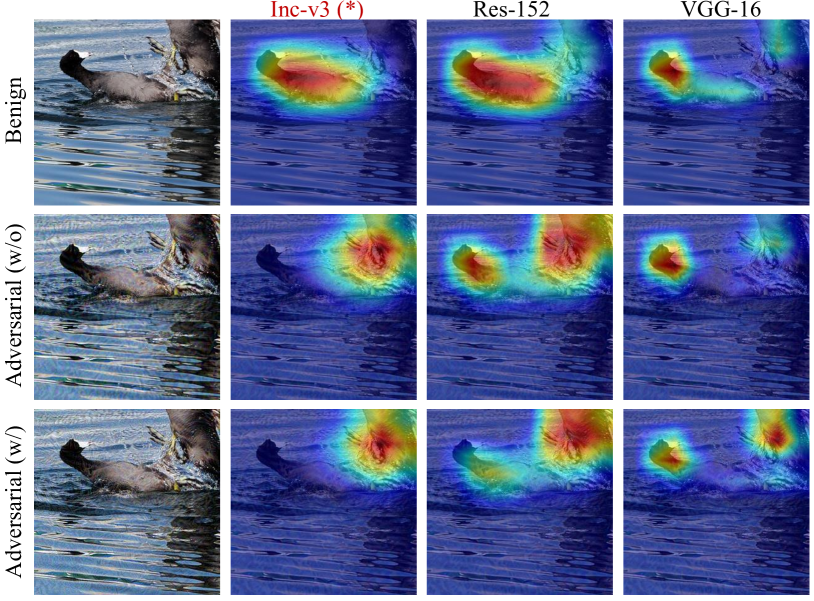
Figure 1. Visualization of attention shift. We apply Eigen-CAM (Muhammad and Yeasin, 2020) to visualize attention maps of benign (1st row) and adversarial images (2nd and 3rd rows) generated by our method without/with SVD. The 1st row shows maps of three representative models (Inception V3, ResNet-152, and VGG-16) on the benign image. The 2nd and 3rd rows show adversarial images generated on the source model (Inception-V3) and transferred to attack the target models (ResNet-152 and VGG-16). The result demonstrates that adversarial examples with SVD are more capable of disturbing the visual attention from the real foreground object to a common trivial region across different models.

Over the past decade, Deep Neural Networks (DNNs) have achieved significant progress in various computer vision tasks, such as, image classification (He et al., 2016), object detection (Ren et al., 2015), and image segmentation (Ronneberger et al., 2015). However, Goodfellow et al. (Goodfellow et al., 2015) have revealed that adding quasi-imperceptible adversarial perturbations into original input images can deceive DNNs into producing incorrect predictions, thus raising severe security issues for many applications, e.g., face recognition (Dong et al., 2019b) and autonomous driving (Kong et al., 2020). Therefore, it is critical to identify the weakness of the DNNs by developing more effective attack methods beforehand, which can subsequently be used to improve the robustness of DNNs.

Compared to white-box attacks, where the structure and the parameters are known to the attacker, black-box attacks have no access to this information. This makes them more practical for real-world applications. Besides, a more severe issue of adversarial examples is their good transferability (Szegedy et al., 2013). As a result, many works (Dong et al., 2018; Xie et al., 2019; Wang et al., 2022) have leveraged the transferability to attack other unknown black-box models. Additionally, there is another type of black-box attack method, i.e., query-based, which conducts several queries to approximate the gradient information for crafting adversarial examples. In this study, we focus on improving the transferability of transfer-based black-box attacks.

Recently, various methods have been developed to improve the transferability of adversarial samples from several different aspects, including gradient-based (Kurakin et al., 2018; Lin et al., 2020), loss function-based (Carlini and Wagner, 2017; Zhao et al., 2021), input transformation-based (Xie et al., 2019; Byun et al., 2022), and feature-based (Huang et al., 2019; Wang et al., 2021a; Zhang et al., 2022). The first three types of methods primarily manipulate either the inputs or outputs of models. In contrast, the last feature-based methods improve the transferability by disrupting the feature maps of intermediate layers in the surrogate model since the important features are typically shared among different models (Wu et al., 2020).

Existing feature-based attacks mainly aim to disturb the neuron activation of adversarial samples compared to original clean samples. The Feature Disruptive Attack (FDA) (Ganeshan et al., 2019) conducts the attack by optimizing the neuron activation towards mean activation in each middle layer. Instead of treating each neuron equally in the FDA, there are some attempts to consider the importance of each neuron for the attack. The Feature Importance-aware Attack (FIA) (Wang et al., 2021a) estimates the importance by computing the gradient with respect to multiple random masked inputs. The Neuron Attribution-based Attack (NAA) (Zhang et al., 2022) calculates neuron importance based on the neuron attribute method (Dhamdhere et al., 2018). Besides, Wu et al. (Wu et al., 2020) leverage the attention map to measure the feature importance and regularize optimization by disturbing the attention map. However, these methods often require significant extra computation for obtaining either neuron or feature importance.

On the other hand, a recent study on domain adaptation (Chen et al., 2019) analyzed deep features from a spectral perspective and found that the eigenvectors with larger singular values contribute the most to generalization across different domains. Besides, Muhammad et al. (Muhammad and Yeasin, 2020) proposed the Eigen-CAM for visualizing the attention map of the last convolutional layer. By projecting feature maps on their largest channel-wise eigenvector, the activation map can robustly and reliably localize the foreground objects as shown in Figure 1 (Row 1st). Accordingly, we assume that the eigenvectors corresponding to the largest singular value can be leveraged to increase the adversarial transferability due to its superior generalization and attention properties.

Inspired by the above findings, we propose a new feature-based attack method that utilizes singular value decomposition (SVD). Specifically, our approach involves selecting a middle layer with sufficient semantic information from the surrogate CNN model and decomposing its feature map by the SVD $\bm{X}=\bm{U}\bm{S}\bm{V}^{T}$. We then only retain the decomposed Top-1 feature with the largest singular value $\bm{Z}=s_{1}\bm{u}_{1}\bm{v}_{1}^{T}$, and forward it in parallel with the original feature $X$ through all subsequent layers to obtain corresponding output logits, respectively. Finally, these two logits are mixed up to compute the loss function and update adversarial examples via back-propagation. Comparing Row 2 and Row 3 in Figure 1, we can find that the adversarial sample learned with the SVD has better transferability than the original adversarial sample without SVD. To evaluate the effectiveness of the proposed method, we conduct extensive experiments in both white-box and box-box settings by using different training baselines.

In summary, the main contributions of this study are as follows:

• We propose a simple and effective feature decomposition adversarial attack method based on SVD to boost transferability by reliably localizing the critical features in the CNN models. Besides, the proposed feature decomposition attack method can be easily integrated into other attack methods to improve their performance.

• Extensive experiments have been conducted to verify the effectiveness of our attack method, which can significantly improve the transferability of adversarial samples against both normally trained CNN models and defense strategies.

2. Related Work

2.1. Adversarial Attacks

In the past few years, many adversarial attack methods (Goodfellow et al., 2015; Carlini and Wagner, 2017; Kurakin et al., 2018; Dong et al., 2018; Du and Pun, 2020; Mingxing et al., 2021; Wang et al., 2022; Zhang et al., 2022; Byun et al., 2022) have been proposed for crafting destructive adversarial samples. Besides, adversarial samples exhibit black-box transferability in which adversarial examples from one source model can be reused to fool other unknown models. Thus, it sparks the research of black-box attacks. To generate more destructive and transferable adversarial examples, many methods have been developed that focus on different aspects. We group them into the following categories.

Gradient-based: This type of method increases transferability through advanced gradient-based optimization. The FGSM (Goodfellow et al., 2015) is the pioneer gradient-based attack method that directly generates adversarial examples in a single-step optimization by maximizing the cross-entropy loss function. I-FGSM (Kurakin et al., 2018) extends the FGSM into an iterative updating method, which iteratively adds the perturbation with a small step size in the gradient direction. MI-FGSM (Dong et al., 2018) incorporates the momentum term into the I-FGSM to encourage a stabilized optimization direction. Similarly, NI-FGSM (Lin et al., 2020) integrates the Nesterov accelerated gradient (NAG) to accumulate the gradients over training iterations. Projected gradient descent (PGD) (Madry et al., 2017) is a variant of FGSM, which includes a random initialization within the allowed norm ball and is then followed by the optimization strategy of I-FGSM. LinBP (Guo et al., 2020) approximates gradients from a smoother surface by skipping over some non-linear activations to reduce the number of non-linear paths in the surrogate model. Huang et al (Huang and Kong, 2022) introduced an integrated gradient to improve transferability, which optimizes the perturbation using a line integral of the gradients from a black reference image to the input image.

Loss-based: Some studies focus on developing new loss functions for optimization to generate adversarial examples. C&W loss (Carlini and Wagner, 2017) directly enlarge the margin distance between the logits of benign examples and the adversarial examples. In (Naseer et al., 2019), a Relativistic Cross-Entropy (RCE) loss is proposed to enforce the confidence between the adversarial sample and the clean sample having a relatively large margin. (Zhao et al., 2021) observed the saturation issue of using the Cross-Entropy loss for crafting targeted adversarial examples and proposes a Logit Loss that is equal to the negative value of target logits for training. For learning disruptive Universal Adversarial Perturbation (UAP), (Zhang et al., 2021) leverages the Cosine Similarity Loss for optimization by minimizing the cosine similarity between the real sample and its adversarial counterpart.

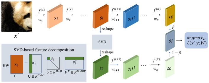
Figure 2. The overall framework of our proposed SVD-based feature decomposition adversarial attack method. The $X_{f}$ is the final logits, retaining logits $Z_{k}$ computed by the decomposed Top-1 singular value-related feature $Z_{l}$ and the original logits $X_{k}$.

Input transformation-based: To further improve the transferability, several input transformation methods have been proposed to augment samples at the input level. For example, the Diverse Input (DI) (Xie et al., 2019) applies random resizing and padding to the input images during each training iteration. The Translation-Invariant (TI) (Dong et al., 2019a) finds that shifting the input images to obtain an ensemble of adversarial images can improve the performance. To further improve the efficiency, the TI method is implemented by convolving the gradient of the input image with a pre-defined kernel. The Scale-Invariant (SI) (Lin et al., 2020) learns the adversarial perturbations over multiple scale copies ($S_{i}(x)=x/2^{i}$) of the input image. The Object-Based Diverse Input (ODI) (Byun et al., 2022) projects the input image onto several 3D objects for data augmentation. Besides, Long et al. (Long et al., 2022) proposes a frequency domain data augmentation for training, and this can significantly improve the transferability. These input transformation-based methods are add-on steps that can be directly integrated into other adversarial attack methods.

Feature-based: Instead of generating adversarial examples mainly based on the final decision of CNN models, some attempts have been made to improve the transferability based on the features of intermediate layers. Intermediate Level Attack (Huang et al., 2019) enhances transferability using a two-step optimization. The first step involves a standard attack, and the second step increases the perturbation on a pre-specified layer of a CNN model along the optimization direction in the previous step. Feature Disruptive Attack (FDA) (Ganeshan et al., 2019) generates adversarial examples by disrupting features at each layer of the CNN. Based on the observation that the classification attention maps of different CNN models are very similar, Attention-guided Transfer Attack (ATA) (Wu et al., 2020) improves the transferability of adversarial samples by further destructing the attention maps. Feature Importance-aware Attack (FIA) (Wang et al., 2021a) uses multiple random masked input images to compute feature importance based on the accumulated gradients w.r.t an intermediate layer, and then compute the perturbation by disrupting the weighted feature map. Neuron Attribution-based Attack (NAA) (Zhang et al., 2022) computes neuron importance in a middle layer based on neuron attributes and conducts the feature-level attacks by weighting neurons.

Compared with other feature-based methods, our method does not actually require explicit computation of the feature importance of different neurons. Instead, the SVD decomposition can implicitly identify important features that improve transferability. Additionally, our proposed approach is an add-on component that can be incorporated into various different attacking methods to enhance their performance.

2.2. Adversarial Defense

Recently, numerous methods have been proposed to mitigate the security issue raised by adversarial attacks. These methods can be mainly divided into adversarial training-based and input pre-processing methods. The adversarial training-based method (Madry et al., 2017) is a simple and effective way of improving the robustness of the model, where the adversarial samples are augmented with the clean training samples to retrain the model. On the other hand, the input pre-processing methods mainly aim to cure the infection of adversarial perturbations before feeding the images into CNNs, e.g., JPEG compression (Guo et al., 2017), random resizing and padding (R&P) (Xie et al., 2017), and high-level representation guided denoiser (HGD) (Lin et al., 2020). Additionally, to further improve defense performance, many works try to combine the benefits of adversarial training and input pre-processing methods, e.g., NeurIPS-r3 solution (Thomas and Elibol, 2017) and Neural Representation Purifier (NRP) (Naseer et al., 2020). In this study, we leverage these defenses to validate the disruptiveness of our proposed adversarial attack.

3. Preliminaries

We consider Convolutional Neural Networks (CNNs) used for image classification as a function $f$, which can be described as a series of successive functions $f=f^{(K)}\circ f^{(K-1)}\circ\cdots\circ f^{(1)}$ with parameters $W=(\textbf{w}_{K},\textbf{w}_{k-1},\cdots,\textbf{w}_{1})$. Here, $f^{(l)}$ is layer $l$, and $\textbf{w}_{l}$ are its corresponding parameters. $K$ represents the total number of layers. Besides, we denote the output of layer $l$ as ${\textbf{X}}_{l}$ for an input image $x$.

Given a CNN model $f$ and a clean image $x$ with ground truth label $y$, our primary goal is to craft an adversarial example $x^{\prime}$ that can mislead the classifier $f$ into making an unexpected prediction. To ensure that the induced perturbation to the original image $x$ is minimally changed, an adversarial example is usually bounded in the $l_{p}$-norm ball centered at $x$ with radius $\epsilon$. Following previous works (Goodfellow et al., 2015; Xie et al., 2019; Gao et al., 2021), we adopt the widely advocated $l_{\infty}$-norm in this work. More formally, it can be summarized as follows:

(1) $$\arg\max f(x^{\prime})\neq y,\quad\mbox{s.t.}\quad||x^{\prime}-x||_{\infty}\leq\epsilon.$$

Let $\mathcal{L}(x^{\prime},y;W)$ represent the loss function for crafting adversarial examples in Eq. 1, which can be formulated as:

(2) $$\arg\max_{x^{\prime}}\mathcal{L}(x^{\prime},y;W),$$

where $\mathcal{L}(x^{\prime},y;W)$ is usually the cross-entropy loss.

In real-world scenarios, the attacker has no access to the parameter $W$ of the victim model $f$. Following the common practice, we fool the victim model based on the transferability of the adversarial examples, crafted by a substitute model. Besides, we enhance transferability based on advanced gradient-based optimization methods, e.g., Iterative-Fast Gradient Sign Method (I-FGSM). The I-FGSM iteratively adds the perturbation with a small step size $\alpha$ in the gradient direction:

(3) $${{x^{\prime}}}_{0}=x,\quad{{x^{\prime}}}_{i+1}={{x}}^{\prime}_{i}+\alpha\cdot\text{sign}(\nabla_{{x^{\prime}}}\mathcal{L}(x^{\prime}_{i},y;W)),$$

where ${x}_{i}^{\prime}$ denotes adversarial image in the $i_{th}$ iteration, and $\alpha=\epsilon/T$ ensures that $x^{\prime}$ is within the $l_{p}$-norm when optimized by a maximum of $T$ iterations.

4. Method

In this section, we introduce our proposed attack method based on the SVD. We extract the Top-1 singular value feature from a middle layer $l$ to obtain more generalized information for boosting the transferability of adversarial examples. Finally, we describe the loss function for optimization.

4.1. Overall architecture

The overall architecture of our proposed feature decomposition attack framework is shown in Fig. 2. For an input image $x$, we pass it through the surrogate CNN model to compute the feature of each layer $f^{(i)}$. In a middle layer $l$, we decompose the corresponding feature $\bm{X}_{l}$ by SVD and obtain the Top-1 feature $\bm{Z}_{l}$ with the largest singular value. Then, the original feature $\bm{X}_{l}$ and the top-1 feature $\bm{Z}_{l}$ are concurrently transmitted to the remaining layers of CNN to compute the corresponding outputs $\bm{X}_{k}$ and $\bm{Z}_{k}$ in two parallel branches, respectively. Finally, we compute the attack loss function based on $\bm{X}_{k}$ and $\bm{Z}_{k}$, and update the adversarial example by gradient backpropagation.

4.2. SVD-based feature decomposition

A recent study (Chen et al., 2019) analyzed the deep feature from a spectral analysis perspective for domain adaptation tasks. After decomposing the feature representation by SVD, the eigenvectors associated with larger singular values usually contribute to generalization in cross-domain classification. On another aspect, (Muhammad and Yeasin, 2020) proposed an Eigen-CAM for visualizing the learned features in a CNN. By projecting the feature map of the last convolutional layer on its largest channel-wise eigenvector, the activation map can robustly and reliably localize the foreground objects without the computation of back-propagation.

To enhance the transferability of attacking unknown black-box CNNs, it is encouraged to address the overfitting issue of adversarial samples biasing towards the training surrogate CNN. Inspired by findings in (Chen et al., 2019; Muhammad and Yeasin, 2020), we also utilize the feature decomposition based on SVD to enhance the adversarial transferability. The detailed computation procedures are as follows.

Given the feature map $\bm{X}_{l}\in R^{C\times H\times W}$ of middle layer $l$, we first reshape it to the size $\mathcal{X}_{l}\in R^{C\times HW}$. Let $M=\min(C,HW)$, we then perform the Singular Value Decomposition (SVD) to decompose the feature into:

(4) $$\mathcal{X}_{l}=\bm{U}\bm{S}\bm{V}^{T},$$

where $\bm{S}\in R^{M\times M}$ is the rectangular diagonal singular value matrix, $\bm{U}\in R^{C\times M}$ is the left orthogonal singular vector matrix, $\bm{V}\in R^{HW\times M}$ is the right orthogonal singular vector matrix.

After the decomposition, we compute the Top-1 decomposed feature $\bm{Z}_{l}$ with respected to the largest singular value $s_{1}$ by:

(5) $$\bm{Z}_{l}=s_{1}\bm{u}_{1}\bm{v}_{1}^{T},$$

where $\bm{u}_{1}$ and $\bm{v}_{1}$ are the corresponding left and right singular vectors, respectively. The $\bm{Z}_{l}$ is reshaped back to $\bm{Z}_{l}\in R^{C\times H\times W}$ and is further used for computing the decomposed logits. Besides, we evaluate the attacking performance of using different Top-$k$ singular value to obtain the decomposed feature, i.e., $\bm{Z}_{l}=\sum_{i=1}^{k}s_{i}\bm{u}_{i}\bm{v}_{i}^{T}$.

4.3. Attacking algorithm

Since our proposed SVD-based feature decomposition can be integrated into different adversarial baselines for crafting the adversarial samples, this section only presents the loss function used for learning the adversarial perturbation in this study.

After getting the Top-1 decomposed feature $\bm{Z}_{l}$, we jointly forward it with $\bm{X}_{l}$ in parallel through the rest of the layers in the CNNs, and we can obtain the output logits $\bm{Z}_{k}$ and $\bm{X}_{K}$, respectively. Then, we combine them jointly to obtain the final logits:

(6) $$\bm{X}_{f}=\beta\bm{X}_{K}+(1-\beta)\bm{Z}_{k},$$

where $\beta$ is a hype-parameter controlling the influence of the decomposed feature.

Based on the fused logits $\bm{X}_{f}$, we can compute the final loss function by the cross-entropy:

(7) $$\mathcal{L}(x^{\prime},y;W)=-\mathds{1}_{y}^{T}\cdot\log\big{(}\text{softmax}(\bm{X}_{f})\big{)},$$

where $y$ is the ground-truth label of the input $x$.

5. Why SVD method is effective?

In this section, we will analyze why incorporating SVD to craft adversarial examples can improve attacking performance. Representation similarity (RS) metrics have been widely used to quantitatively compare the activations of different sets of neurons on a given dataset. Following (Cianfarani et al., 2022), we leverage the linear Centred Kernel Alignment (CKA) to measure the RS between the clean samples and adversarial samples. The linear CKA is computed as follows:

(8) $$\text{CKA}_{L}(\bm{X},\bm{Y})=\frac{||\bm{Y}^{T}\bm{X}||^{2}_{F}}{||\bm{X}^{T}\bm{X}||_{F}||\bm{Y}^{T}\bm{Y}||_{F}},$$

where $\bm{X}\in\mathbb{R}^{n\times d_{1}}$ and $\bm{Y}\in\mathbb{R}^{n\times d_{2}}$ are two feature activations of a set with $n$ samples. The $d_{1}$ and $d_{2}$ are the corresponding feature dimensions. To compute the linear CKA, we craft adversarial examples for 1000 images from ImageNet-Compatible Dataset by using Inc-v3 as the source model. The S²I-TI-DIM (Long et al., 2022) is used for optimization. More training details can be found in the experiments.

First, we compute the linear CKA between the features of clean samples and adversarial samples from the source Inc-v3 model. At layer $l$, we denote the features of all clean samples, adversarial samples (w/o SVD), and adversarial samples (w/ SVD) as $\bm{X}\in\mathbb{R}^{1000\times d_{l}}$, $\tilde{\bm{X}}\in\mathbb{R}^{1000\times d_{l}}$, $\tilde{\bm{X}}_{svd}\in\mathbb{R}^{1000\times d_{l}}$, where $d_{l}$ is the feature dimension at layer $l$. Then, we compute $\text{CKA}_{L}(\bm{X},\tilde{\bm{X}})$ and $\text{CKA}_{L}(\bm{X},\tilde{\bm{X}}_{svd})$. As shown in Table 1, we can find that the similarities between the representations of clean and adversarial samples (w/ SVD) are much smaller than without SVD, particularly at those higher layers. These results indicate that the adversarial examples crafted by using SVD are more disruptive in terms of attacking the white-box model.

Additionally, according to  (Cianfarani et al., 2022), ”high transferability indicates that the target network has learned similar decision boundary”. Therefore, when the representations that are correlated with the classification are more similar, the adversarial examples trained on the source models are easier to transfer to the target models. Specifically, we compute the linear CKA at the final global pooling layer and FC layer. These layers are highly correlated with the classification since different models have different architectures. In this part, we directly use the adversarial samples generated by Inc-v3 to compute the features from Inc-v3, ResNet-152, and VGG-16. As shown in Table 2, the linear CKA between Inc-v3 and ResNet-152 at Pool and FC layers for 1000 clean samples are 0.3769 and 0.4407, respectively. The linear CKA of adversarial samples (w/o SVD) will decrease to 0.2066 and 0.2182. On the other hand, we can find that the linear CKA of adversarial samples (w/ SVD) will slightly increase to 0.2273 and 0.2447, which means the representation of adversarial samples (w/ SVD) transferred from Inc-v3 to ResNet-152 are more similar than adversarial samples (w/o SVD). Besides, a similar finding can be found between Inc-v3 and VGG-16. These results indicate that our proposed SVD-based optimation methods can enhance the classification-related representation similarity of the adversarial examples between the source model and the target model, thereby improving transferability.

Upon analyzing the representation similarity using linear CKA, we can observe that crafting adversarial examples using SVD is effective in disrupting feature activations in the white-box model. Additionally, this also can enhance the transferability of adversarial samples for attacking black-box models.

Table 1. The linear CKA between the features of clean samples and adversarial samples computed from different layers of the source Inc-v3 model.

	Conv2d_4a	Mixed_5d	Mixed_6e	Mixed_7c	Pool	FC
w/o	0.9279	0.7183	0.6138	0.2765	0.1278	0.0885
w/	0.9251	0.6902	0.4697	0.2120	0.1140	0.0731

Table 2. The linear CKA between the features under the setting of transferring the adversarial examples crafted by Inc-v3 to ResNet-152 and VGG-16.

	Inc-v3 $\rightarrow$ ResNet-152			Inc-v3 $\rightarrow$ VGG-16
	Clean	Adv (w/o)	Adv (w/)	Clean	Adv (w/o)	Adv (w/)
Pool	0.3769	0.2066	0.2273	0.2160	0.1107	0.1165
FC	0.4407	0.2182	0.2447	0.3196	0.1793	0.1896

6. Experiments

6.1. Experimental Setup

Dataset: Following previous studies (Dong et al., 2018; Long et al., 2022), we conduct the experiments on the challenge ImageNet-Compatible Dataset. The dataset contains 1,000 images with 1,000 unique class labels that correspond to the original ImageNet dataset.

Models: In this study, we utilize four normally trained ImageNet CNN models as source models to craft adversarial examples, i.e., Inception-v3 (Inc-v3) (Szegedy et al., 2016), Inception-v4 (Inc-v4) (Szegedy et al., 2017), Inception-Resnet-v2 (IncRes-v2) (Szegedy et al., 2017) and Resnet-v2-152 (Res-152) (He et al., 2016). To evaluate the performance of the adversarial samples, we use the four training source models and Resnet-v2-50 (Res-50) and Resnet-v2-101 (Res-101) as victim models. Besides, for further evaluation of attacking defense models, we select four adversarially trained models based on PGD-AT (Madry et al., 2017) and Ensemble Adversarial Training (tramer2017ensemble), which augments a model’s training data with adversarial examples crafted on other static pre-trained models for yielding models with stronger robustness to black-box attacks. Specifically, adversarially trained models include an adversarially trained Inception-v3 model (Inc-v3_adv), an ensemble of three adversarially trained Inception-v3 models (Inc-v3_ens3), an ensemble of four adversarially trained Inception-v3 models (Inc-v3_ens4) and an ensemble of three adversarially trained Inception-Resnet-v2 models (IncRes-v2_ens). Additionally, we select advanced defense methods that cover random resizing and padding (R&P) (Xie et al., 2017), NIPS-r3 (Thomas and Elibol, 2017), HGD (Lin et al., 2020), JPEG (Guo et al., 2017), randomized smoothing (RS) (Jia et al., 2019) and NRP (Naseer et al., 2020) ), which are robust against black-box attacks.

Baseline Method: To thoroughly evaluate performance, we integrate our method into various well-known adversarial attacking baselines, including DI-FGSM (Xie et al., 2019), TI-FGSM (Dong et al., 2019a), MI-FGSM (Dong et al., 2018), VT-FGSM (Wang and He, 2021), SI-NI-FGSM (Lin et al., 2020), PI-TI-DI-FGSM (Gao et al., 2020), and Admix (Wang et al., 2021b). Additionally, we incorporate our method into one current SOAT attacking method S²-I-FGSM (Long et al., 2022), which adopts a frequency-based spectral transformation for data augmentation. Besides, we combine these simple baselines jointly to construct stronger disruptive attacking baselines.

Table 3. The attack success rates ($\%$) on six normally trained models. The adversarial examples are crafted via Inc-v3, Inc-v4, IncRes-v2, and Res-152, respectively.

Model	Attack	SVD	Inc-v3	Inc-v4	IncRes-v2	Res-152	Res-50	Res-101	Avg
Inc-v3	MI-FGSM	w/o	100.0	50.6	45.8	41.2	47.1	42.1	54.5
		w/	100.0	55.2	52.8	44.9	49.9	46.5	58.2 ($\uparrow 3.7$)
	DI-FGSM	w/o	99.9	49.6	37.7	32.7	37.4	33.5	48.5
		w/	99.5	53.1	44.7	34.2	43.0	37.6	52.0 ($\uparrow 3.5$)
	S2I-FGSM	w/o	99.7	63.6	57.5	49.9	56.5	52.0	63.2
		w/	99.8	69.8	65.9	57.2	64.2	60.1	69.5 ($\uparrow 6.3$)
	SI-NI-FGSM	w/o	100.0	76.9	74.7	68.0	72.2	69.1	76.8
		w/	100.0	80.2	79.1	70.7	76.2	72.3	79.8 ($\uparrow 3.0$)
	VT-MI-FGSM	w/o	100.0	75.0	69.9	62.6	66.8	62.3	72.8
		w/	99.8	80.6	78.7	69.0	73.7	70.6	78.7 ($\uparrow 5.9$)
Inc-v4	MI-FGSM	w/o	60.7	99.9	45.5	42.3	47.7	43.5	56.6
		w/	63.5	100.0	48.7	44.9	50.1	46.3	58.9 ($\uparrow 2.3$)
	DI-FGSM	w/o	52.5	99.2	36.0	29.9	32.7	30.5	46.8
		w/	56.0	99.5	40.2	32.6	39.2	33.7	50.2 ($\uparrow 3.4$)
	S2I-FGSM	w/o	71.5	99.6	55.4	49.0	57.1	48.9	63.6
		w/	76.1	99.6	62.6	54.3	60.4	55.3	68.1 ($\uparrow 4.5$)
	SI-NI-FGSM	w/o	86.0	100.0	79.1	73.6	77.1	73.7	81.6
		w/	87.1	100.0	81.4	75.3	79.6	75.9	83.2 ($\uparrow 1.6$)
	VT-MI-FGSM	w/o	80.1	99.8	70.6	64.2	65.8	63.8	74.1
		w/	85.0	99.9	76.5	69.9	71.4	68.6	78.6 ($\uparrow 4.5$)
IncRes-v2	MI-FGSM	w/o	60.2	53.4	99.2	44.1	49.6	46.7	58.9
		w/	71.5	61.2	99.7	50.8	57.4	54.8	65.9 ($\uparrow 7.0$)
	DI-FGSM	w/o	56.3	51.6	97.7	37.1	39.8	36.3	53.1
		w/	64.2	58.8	98.9	39.6	46.0	41.9	58.2 ($\uparrow 5.1$)
	S2I-FGSM	w/o	77.3	68.0	98.4	56.1	62.4	58.1	70.1
		w/	80.0	72.3	99.1	60.9	66.6	62.6	73.6 ($\uparrow 3.5$)
	SI-NI-FGSM	w/o	86.6	84.0	99.8	76.5	80.0	77.5	84.1
		w/	90.0	87.8	100.0	81.8	84.6	83.6	88.0 ($\uparrow 3.9$)
	VT-MI-FGSM	w/o	81.1	76.6	99.0	66.7	70.1	68.7	77.0
		w/	88.0	84.9	99.7	77.1	79.2	78.4	84.6 ($\uparrow 7.6$)
Res-152	MI-FGSM	w/o	56.3	50.8	46.0	99.4	82.9	86.2	70.3
		w/	63.9	53.9	50.1	99.4	88.0	89.1	74.1 ($\uparrow 3.8$)
	DI-FGSM	w/o	55.9	53.2	46.3	99.6	83.2	84.3	70.4
		w/	61.4	56.9	50.4	99.5	86.3	88.5	73.8 ($\uparrow 3.4$)
	S2I-FGSM	w/o	66.6	63.3	57.6	99.8	93.5	93.9	79.1
		w/	71.6	64.9	62.5	99.8	95.2	95.2	81.5 ($\uparrow 2.4$)
	SI-NI-FGSM	w/o	76.3	72.5	72.6	99.8	94.2	95.3	85.1
		w/	78.5	76.5	75.9	99.9	95.5	95.9	87.0 ($\uparrow 1.9$)
	VT-MI-FGSM	w/o	73.7	68.7	65.8	99.5	93.2	93.8	82.5
		w/	80.2	75.9	73.4	99.5	93.9	95.7	86.4 ($\uparrow 3.9$)

Table 4. The attack success rates (%) on ten defenses. The adversarial examples are crafted via Inc-v3, Inc-v4, IncRes-v2 and Res-152.

Model	Attack	SVD	Inc-v3adv	Inc-v3ens3	Inc-v3ens4	IncRes-v2ens	HGD	R&P	NIPS-r3	JPEG	RS	NRP	AVG.
Inc-v3	TI-DIM	w/o	45.5	43.1	43.2	28.6	36.2	30.0	35.4	54.6	36.2	24.9	37.8
		w/	49.2	48.4	45.5	32.0	40.0	34.3	41.2	59.8	39.0	24.3	41.4
	PI-TI-DI-FGSM	w/o	44.6	44.0	46.0	33.4	32.4	33.7	37.0	46.7	64.7	36.9	41.9
		w/	48.0	46.6	47.9	35.8	34.2	36.5	40.3	50.2	66.7	38.9	44.5
	VT-TI-DIM	w/o	64.3	65.0	64.3	47.6	58.8	51.7	57.6	74.9	42.6	35.2	56.2
		w/	67.9	69.4	67.3	51.9	61.7	53.5	62.3	80.2	45.1	37.8	59.7
	Admix-TI-DIM	w/o	77.0	75.6	73.9	60.0	69.6	62.2	70.3	84.7	55.9	46.3	67.6
		w/	81.6	82.7	79.3	64.8	73.4	57.5	75.5	88.2	58.9	47.3	70.9
	S2I-TI-DIM	w/o	82.8	81.9	79.2	68.8	77.1	70.0	75.9	87.2	61.2	57.2	74.1
		w/	85.8	84.8	83.5	72.9	80.6	75.1	80.1	88.9	64.4	59.1	77.5
Inc-v4	TI-DIM	w/o	38.8	38.9	37.1	29.1	36.3	29.9	33.4	48.7	35.9	19.2	34.7
		w/	41.3	42.3	41.6	29.7	37.0	30.8	36.2	53.3	37.5	21.3	37.1
	PI-TI-DI-FGSM	w/o	40.6	41.6	44.2	34.4	31.7	33.1	32.0	45.4	63.5	34.2	40.1
		w/	43.6	44.8	45.8	35.2	33.4	35.6	37.8	47.7	65.5	36.9	42.6
	VT-TI-DIM	w/o	57.9	61.4	59.7	48.4	58.8	51.9	55.1	70.8	41.3	32.0	53.7
		w/	61.3	64.7	62.7	52.8	61.8	53.6	59.1	76.1	42.0	36.1	57.0
	Admix-TI-DIM	w/o	77.3	78.7	74.5	65.7	75.8	69.2	74.0	83.7	54.5	49.1	70.3
		w/	78.7	81.2	77.0	69.0	76.7	72.3	75.8	86.2	56.0	47.6	72.1
	S2I-TI-DIM	w/o	80.2	80.8	77.7	71.0	77.2	72.4	76.4	84.7	60.4	56.5	73.7
		w/	82.1	82.2	78.8	72.9	78.3	74.3	78.2	86.3	63.6	59.0	75.6
IncRes-v2	TI-DIM	w/o	43.1	46.4	40.9	39.4	43.4	39.0	41.5	56.6	36.7	22.2	40.9
		w/	52.3	56.8	50.2	41.6	50.2	45.2	50.9	68.6	40.4	26.9	48.3
	PI-TI-DI-FGSM	w/o	47.8	48.7	49.5	45.6	39.4	45.8	46.5	51.1	66.3	40.9	48.2
		w/	54.9	54.7	56.1	50.3	45.7	50.2	51.6	56.1	70.3	45.8	53.6
	VT-TI-DIM	w/o	61.8	66.4	61.7	59.5	64.0	61.4	62.1	72.6	43.4	35.4	58.8
		w/	72.8	78.0	71.7	67.8	72.4	69.7	73.1	84.7	47.4	42.8	68.0
	Admix-TI-DIM	w/o	83.5	84.8	83.4	79.0	82.9	81.6	82.3	88.5	64.0	61.2	79.1
		w/	88.0	89.3	87.5	85.1	86.4	84.6	86.8	92.4	65.5	62.2	82.8
	S2I-TI-DIM	w/o	81.8	81.8	78.5	78.6	79.9	79.1	80.4	85.0	63.0	60.7	76.9
		w/	88.7	88.7	85.7	85.0	86.2	85.2	87.1	91.0	70.5	66.3	83.4
Res-152	TI-DIM	w/o	55.7	55.9	52.5	43.4	55.3	46.5	51.9	66.0	46.5	31.4	50.5
		w/	58.7	58.7	55.3	43.6	56.4	47.2	55.6	70.7	48.4	33.0	52.8
	PI-TI-DI-FGSM	w/o	53.1	52.7	55.4	46.8	42.2	46.8	51.0	54.3	71.2	47.2	52.1
		w/	56.0	57.2	59.1	49.1	47.4	49.4	51.6	58.5	73.0	46.9	54.8
	VT-TI-DIM	w/o	67.9	73.4	69.3	60.5	70.4	64.9	68.3	80.7	52.7	43.0	65.1
		w/	74.2	77.1	72.6	64.8	74.8	67.7	71.8	83.2	55.6	46.8	68.9
	Admix-TI-DIM	w/o	79.0	83.0	78.7	70.4	80.2	74.8	78.3	86.4	65.2	57.7	75.4
		w/	81.1	86.1	82.1	73.2	81.4	77.5	81.0	88.4	67.4	59.3	77.8
	S2I-TI-DIM	w/o	86.8	86.6	83.9	79.0	85.1	80.9	85.3	89.3	72.6	68.6	81.8
		w/	88.8	87.8	85.2	79.9	85.9	83.1	85.8	91.3	75.0	69.5	83.2

Parameter: In all experiments, the maximum perturbation is $\epsilon=16$, the iteration is $T=10$ and the step size is $\alpha=\epsilon/T$. For MI-FGSM (Dong et al., 2018), we set the decay factor to $\mu=1.0$. For DI-FGSM (Xie et al., 2019), we set the transformation probability to $p=0.5$. For TI-FGSM (Dong et al., 2019a), we set the kernel length to $k=7$. For VT-FGSM (Wang and He, 2021), we set the hyper-parameter to $\beta=1.5$, and the number of sampling examples is 20. For SI-NI-FGSM (Lin et al., 2020), we set the number of copies to $m_{1}=5$. For Admix (Wang et al., 2021b), we set number of copies to $m_{1}=5$, the sample number to $m_{2}=3$, and the admix ratio $\eta=0.2$. For PI-TI-DI-FGSM (Gao et al., 2020), we set the amplification factor to $\beta=10$, the project factor to $\gamma=16$ and the kernel to length $k_{w}=7$. For S²-I-FGSM (Long et al., 2022), we set the tuning factor for $\mathcal{M}$ as $\rho=0.5$, and the number of spectrum transformations as $N=20$. For our proposed SVD-based attacks, the Top-$k$ decomposed feature is $k=1$ and the hyperparameter is $\beta=0.5$. The middle layers for the SVD-based feature decomposition are Mixed-6e for Inception-v3 (Incv3), the last Inception-B blocks of Mixed-6b for Inception-v4 (Inc-v4), the Mixed-6a for Inception-Resnet-v2 (IncRes-v2), and the last layer of block3 in Layer4 for Resnet-v2-152 (Res-152), respectively.

6.2. Attack Normally Trained Models

In this section, we verify the effectiveness of our method against the normally trained models by training the adversarial samples with five different baselines. Based on the results in Table 3, we can make the following findings: 1) For each source model, there are significant improvements in performance when comparing the results of different baselines with SVD to baselines without SVD. For example, when Inc-v3 is used as the source model, average attack success rates increase by 3.7% (MI-FGSM), 3.5% (DI-FGSM), 6.3% (S²I-FGSM), 3.0% (SI-NI-FGSM), and 5.9% (VT-MI-FGSM). 2) When attacking black-box models, the adversarial transferability is also significantly improved after applying SVD. For instance, when VT-MI-FGSM and IncRes-v2 are used as the baseline and the substitute model, attack success rates increase from 81.1% to 88.0%, 76.6% to 84.9%, 66.7% to 77.1%, and 70.1% to 79.2% for transferring attack Inc-v3, Inc-v4, Res-152, and Res-50, respectively.

These findings can validate the effectiveness of our proposed method in improving attack performance against normally trained models. Moreover, when combined with existing attacks, it can further enhance the black-box transferability of adversarial examples.

6.3. Attack Defense Models

To further evaluate the effectiveness of our method, we evaluate the attack success rates against ten different defense strategies, including four adversarially trained models (Inc-v3_adv, Inc-v3_ens3, Inc-v3_ens4, IncRes-v2_ens) and six more advanced methods (HGD, R&P, NIPS-r3, RS, JPEG, NRP). As shown in Table 4, we can find that the proposed method significantly improves performance across source models with diverse training baselines. For example, the average attack success rates of Inc-v3 with TI-DIM, PI-TI-DI-FGSM, VT-TI-DIM, Admix-TI-DIM, and S²I-TI-DIM are increased by 3.6%, 2.6%, 3.5%, 3.4%, and 3.4%, respectively. The results indicate that the Top-1 decomposed feature contributes significantly to the final prediction. However, current defense strategies do not leverage these features to enhance robustness.

6.4. Analysis of computational cost

We calculate the additional computation cost for different baselines using Inc-v3 as the source model when attacking the 1000 images from the ImageNet-Compatible dataset. The results are presented in Table 8. From the table, we can observe that our proposed SVD method introduces an additional computation cost of approximately 25-30% for different baselines.

Table 5. The training cost for different baselines of attacking 1000 images from ImageNet-Compatible dataset with and without the proposed SVD-based attack

SVD	MI-FGSM	DI-FGSM	S2I-FGSM	SI-NI-FGSM	VT-MI-FGSM	TI-DIM	PI-TI-DI-FGSM	SI-NI-TI-DIM	VT-TI-DIM	Admix-TI-DIM	S2I-TI-DIM
w/o	23.39s	27.60s	723.84s	110.09s	452.02s	27.83s	40.58s	125.96s	525.35s	348.98s	815.24s
w/	30.02s	34.98s	890.65s	143.37s	594.03s	35.16s	50.23s	164.40s	684.05s	438.35s	998.17s

6.5. Image Quality of Adversarial Examples

We further compute the SSIM (wang2004image) scores between the original samples and the adversarial samples generated using the Inc-v3 model under different baselines, both with and without our proposed method. SSIM is a popular metric for evaluating image quality, a large SSIM score indicates better quality and less distortion. As shown in Table 6, we can find that SSIM scores obtained without and with our proposed method are very similar. This suggests that our proposed method does not significantly alter the perceptual similarity between the original and adversarial samples.

Table 6. The SSIM between the original samples and the adversarial samples trained by different baselines without and with our proposed method.

SVD	MI-FGSM	DI-FGSM	S2I-FGSM	SI-NI-FGSM	VT-MI-FGSM	TI-DIM	PI-TI-DI-FGSM	SI-NI-TI-DIM	VT-TI-DIM	Admix-TI-DIM	S2I-TI-DIM
w/o	0.8336	0.9505	0.9407	0.8313	0.8389	0.8112	0.7410	0.8110	0.8260	0.8079	0.8043
w/	0.8332	0.9500	0.9425	0.8294	0.8617	0.8109	0.7414	0.8093	0.8444	0.8068	0.8034

6.6. Ablation Study

Target Layer for Decomposition: Firstly, we evaluate the performance using different layers for SVD feature decomposition. In Fig. 3 (a) and (b), we plot the transfer attack success rate using Inc-v3 and Res-152 as the source models, respectively. For each source model, we compare four layers at four convolutional blocks with different feature resolutions. As shown in Fig. 3, we can find that the best performance is achieved at Mixed-6e for Inception-v3 and Layer 3 for ResNet-152. The main reason for this phenomenon is mainly due to that the first two layers have high-resolution and less semantic information. The Mixed-7c and Layer-4 are the last convolutional layers in the Inc-v3 and Res-152 and have less generalization ability. And the decomposed feature with the largest singular value for the last layer is relatively close to the original features, which weakens the contribution of the logits combination.

Parameter: The trade-off influence of the hyperparameter $\beta$ for the Inc-v3 as source model is shown in Fig. 4(a). We can find that the attack success rates increase along with the increment of $\beta$. The overall best performance is achieved at around $\beta=0.5$ for all five black-box models. When $\beta$ is increased further, the attack success rates decrease, indicating that using only the Top-1 decomposed feature is insufficient to achieve better performance. Besides, when $\beta=0$, original features are not utilized, resulting in significantly lower performance than other values. At $\beta=1$, SVD-based features are not utilized. Therefore, these results suggest the original feature is crucial for achieving better-attacking performance.

Top-$k$: In Fig. 4(b), we depict the performance of transferability under Top-$k$ decomposed feature $\bm{Z}_{l}=\sum_{i=1}^{k}s_{i}\bm{u}_{i}\bm{v}_{i}^{T}$. Compared with the original feature (i.e., Top-$0$), we can find that using the Top-1 decomposed feature can significantly boost the attack success rates in all models. However, performance will start to decrease when using Top-$k$ $(k>2)$ decomposed features. Besides, the attack success rates fluctuate around a certain value when $k>=5$, since $\sum_{i=1}^{k}s_{i}\bm{u}_{i}\bm{v}_{i}^{T}$ gradually equals to the original feature.

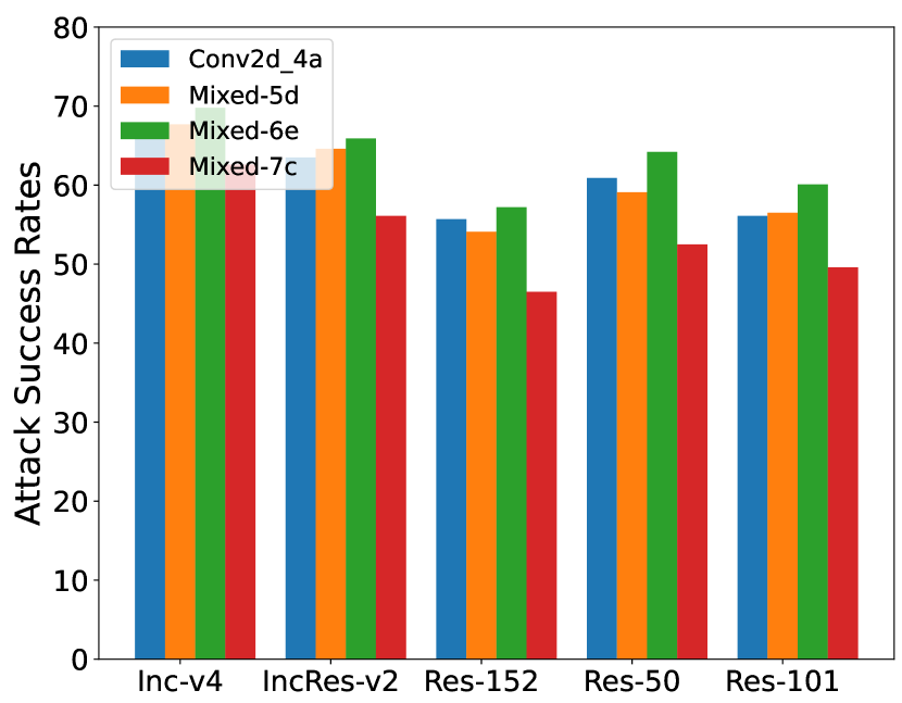
(a) Inception-v3

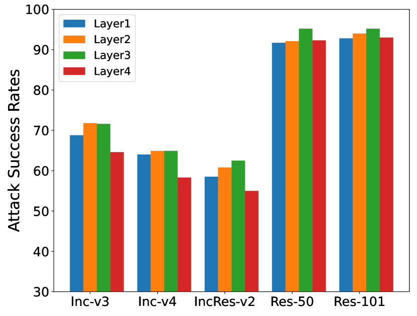
(b) ResNet-152

Figure 3. The black-box performance of using different layers for feature decomposition.

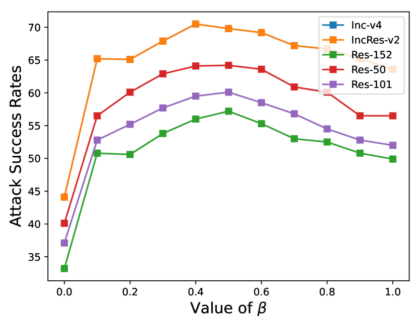
(a) Sensitivity of Parameter $\beta$

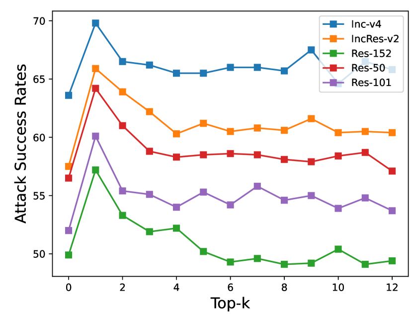
(b) Influence of Top-$k$

Figure 4. Ablation studies of different hyper-parameters against Inception-v3 in the black-box setting.

6.7. Comparison with feature-based methods

In this part, we compare our method with other feature-based methods in terms of both attack success rates and training costs. We craft adversarial examples using the same settings and data augmentation as NAA (Zhang et al., 2022). Based on Table. 7, our method can achieve superior performance in terms of attack success rate compared to the FDA (Ganeshan et al., 2019), FIA (Wang et al., 2021a), and NAA (Zhang et al., 2022) methods. Besides, we compare the total training cost of using Inc-v3 as the source model on a 2080Ti GPU across 1000 images with other feature-based methods. As shown in Table 8, our method is more efficient than the FIA (Wang et al., 2021a), NAA (Zhang et al., 2022), and FDA (Ganeshan et al., 2019), which only requires 1029s for training.

Table 7. Comparing our method with feature-based SOTA methods. The attack success rates (%) on four undefended models and four adversarially trained models.

Model	Attack	Inc-v3	Inc-v4	IncRes-v2	Res-152	Inc-v3adv	Inc-v3ens3	Inc-v3ens4	IncRes-v2ens
Inc-v3	FDA	81.3	42.9	36.0	35.4	19.3	8.9	6.4	2.3
	FIA	98.3	83.2	79.1	71.6	53.3	36.1	37.0	20.0
	NAA	98.1	85.0	82.4	77.1	61.5	50.5	50.8	31.5
	Ours	99.8	87.8	85.2	80.7	64.2	61.2	58.8	38.6
Inc-v4	FDA	84.8	99.6	71.9	68.7	27.9	18.4	17.2	7.3
	FIA	84.1	95.7	78.6	72.0	45.3	38.0	37.2	19.4
	NAA	86.0	96.5	81.0	75.5	52.4	50.5	49.4	30.8
	Ours	90.5	99.5	86.3	80.9	60.8	65.7	63.4	48.1
IncRes-v2	FDA	69.3	67.7	78.3	56.3	36.4	16.2	22.3	17.9
	FIA	81.6	77.1	88.7	71.0	63.8	49.8	46.6	34.1
	NAA	82.4	78.0	93.0	74.4	64.9	60.0	56.7	47.5
	Ours	92.9	92.2	99.3	88.0	76.7	78.0	74.7	70.4
Res-152	FDA	83.9	84.1	73.9	89.1	51.2	27.9	23.6	11.5
	FIA	83	81.6	78.4	98.9	58.2	49.1	44.9	29.3
	NAA	85.9	85.9	83.6	98.2	66.1	61.6	59.2	46.7
	Ours	86.4	84.8	83.1	99.9	70.7	70.4	67.6	57.2

Table 8. The training cost comparison of our method with other feature-based methods.

Method	FDA (Ganeshan et al., 2019)	FIA (Wang et al., 2021a)	NAA (Zhang et al., 2022)	Ours
Cost Time (s)	1421	7081	7163	1029

7. Conclusion

In this paper, we propose the SVD feature decomposition-based attack method. Incorporating decomposed features related to the largest singular value into the attack can intrinsically leverage the advantages of using more generalizable features and attentively localize the foreground object. Extensive experiments demonstrate that the proposed attack method can significantly boost the transferability for attacking both black-box models and defense strategies. On the other aspects, we could consider maintaining the clean singular vectors corresponding to the largest singular value for building more robust defense models.

References

- (1)
- Byun et al. (2022) Junyoung Byun, Seungju Cho, Myung-Joon Kwon, Hee-Seon Kim, and Changick Kim. 2022. Improving the Transferability of Targeted Adversarial Examples through Object-Based Diverse Input. In CVPR. 15244–15253.
- Carlini and Wagner (2017) Nicholas Carlini and David Wagner. 2017. Towards evaluating the robustness of neural networks. In IEEE Symposium on Security and Privacy. 39–57.
- Chen et al. (2019) Xinyang Chen, Sinan Wang, Mingsheng Long, and Jianmin Wang. 2019. Transferability vs. discriminability: Batch spectral penalization for adversarial domain adaptation. In ICML. 1081–1090.
- Cianfarani et al. (2022) Christian Cianfarani, Arjun Nitin Bhagoji, Vikash Sehwag, Ben Zhao, Heather Zheng, and Prateek Mittal. 2022. Understanding robust learning through the lens of representation similarities. NeurIPS 35 (2022), 34912–34925.
- Dhamdhere et al. (2018) Kedar Dhamdhere, Mukund Sundararajan, and Qiqi Yan. 2018. How important is a neuron? arXiv preprint arXiv:1805.12233 (2018).
- Dong et al. (2018) Yinpeng Dong, Fangzhou Liao, Tianyu Pang, Hang Su, Jun Zhu, Xiaolin Hu, and Jianguo Li. 2018. Boosting adversarial attacks with momentum. In CVPR. 9185–9193.
- Dong et al. (2019a) Yinpeng Dong, Tianyu Pang, Hang Su, and Jun Zhu. 2019a. Evading defenses to transferable adversarial examples by translation-invariant attacks. In CVPR. 4312–4321.
- Dong et al. (2019b) Yinpeng Dong, Hang Su, Baoyuan Wu, Zhifeng Li, Wei Liu, Tong Zhang, and Jun Zhu. 2019b. Efficient decision-based black-box adversarial attacks on face recognition. In CVPR. 7714–7722.
- Du and Pun (2020) Xia Du and Chi-Man Pun. 2020. Adversarial image attacks using multi-sample and most-likely ensemble methods. In ACM MM. 1634–1642.
- Ganeshan et al. (2019) Aditya Ganeshan, Vivek BS, and R Venkatesh Babu. 2019. Fda: Feature disruptive attack. In ICCV. 8069–8079.
- Gao et al. (2021) Lianli Gao, Yaya Cheng, Qilong Zhang, Xing Xu, and Jingkuan Song. 2021. Feature space targeted attacks by statistic alignment. arXiv preprint arXiv:2105.11645 (2021).
- Gao et al. (2020) Lianli Gao, Qilong Zhang, Jingkuan Song, Xianglong Liu, and Heng Tao Shen. 2020. Patch-wise attack for fooling deep neural network. In ECCV. 307–322.
- Goodfellow et al. (2015) Ian J Goodfellow, Jonathon Shlens, and Christian Szegedy. 2015. Explaining and harnessing adversarial examples. In ICLR.
- Guo et al. (2017) Chuan Guo, Mayank Rana, Moustapha Cisse, and Laurens Van Der Maaten. 2017. Countering adversarial images using input transformations. arXiv preprint arXiv:1711.00117 (2017).
- Guo et al. (2020) Yiwen Guo, Qizhang Li, and Hao Chen. 2020. Backpropagating linearly improves transferability of adversarial examples. NeurIPS 33 (2020), 85–95.
- He et al. (2016) Kaiming He, Xiangyu Zhang, Shaoqing Ren, and Jian Sun. 2016. Deep residual learning for image recognition. In CVPR. 770–778.
- Huang et al. (2019) Qian Huang, Isay Katsman, Horace He, Zeqi Gu, Serge Belongie, and Ser-Nam Lim. 2019. Enhancing adversarial example transferability with an intermediate level attack. In ICCV. 4733–4742.
- Huang and Kong (2022) Yi Huang and Adams Wai-Kin Kong. 2022. Transferable adversarial attack based on integrated gradients. ICLR (2022).
- Jia et al. (2019) Jinyuan Jia, Xiaoyu Cao, Binghui Wang, and Neil Zhenqiang Gong. 2019. Certified robustness for top-k predictions against adversarial perturbations via randomized smoothing. arXiv preprint arXiv:1912.09899 (2019).
- Kong et al. (2020) Zelun Kong, Junfeng Guo, Ang Li, and Cong Liu. 2020. Physgan: Generating physical-world-resilient adversarial examples for autonomous driving. In CVPR. 14254–14263.
- Kurakin et al. (2018) Alexey Kurakin, Ian J Goodfellow, and Samy Bengio. 2018. Adversarial examples in the physical world. In Artificial intelligence safety and security. 99–112.
- Lin et al. (2020) Jiadong Lin, Chuanbiao Song, Kun He, Liwei Wang, and John E Hopcroft. 2020. Nesterov accelerated gradient and scale invariance for adversarial attacks. In ICLR.
- Long et al. (2022) Yuyang Long, Qilong Zhang, Boheng Zeng, Lianli Gao, Xianglong Liu, Jian Zhang, and Jingkuan Song. 2022. Frequency domain model augmentation for adversarial attack. In ECCV. 549–566.
- Madry et al. (2017) Aleksander Madry, Aleksandar Makelov, Ludwig Schmidt, Dimitris Tsipras, and Adrian Vladu. 2017. Towards deep learning models resistant to adversarial attacks. arXiv preprint arXiv:1706.06083 (2017).
- Mingxing et al. (2021) Duan Mingxing, Kenli Li, Lingxi Xie, Qi Tian, and Bin Xiao. 2021. Towards multiple black-boxes attack via adversarial example generation network. In ACM MM. 264–272.
- Muhammad and Yeasin (2020) Mohammed Bany Muhammad and Mohammed Yeasin. 2020. Eigen-cam: Class activation map using principal components. In IJCNN. 1–7.
- Naseer et al. (2020) Muzammal Naseer, Salman Khan, Munawar Hayat, Fahad Shahbaz Khan, and Fatih Porikli. 2020. A self-supervised approach for adversarial robustness. In CVPR. 262–271.
- Naseer et al. (2019) Muhammad Muzammal Naseer, Salman H Khan, Muhammad Haris Khan, Fahad Shahbaz Khan, and Fatih Porikli. 2019. Cross-domain transferability of adversarial perturbations. NeurIPS (2019).
- Ren et al. (2015) Shaoqing Ren, Kaiming He, Ross Girshick, and Jian Sun. 2015. Faster r-cnn: Towards real-time object detection with region proposal networks. NeurIPS (2015).
- Ronneberger et al. (2015) Olaf Ronneberger, Philipp Fischer, and Thomas Brox. 2015. U-net: Convolutional networks for biomedical image segmentation. In MICCAI. 234–241.
- Szegedy et al. (2017) Christian Szegedy, Sergey Ioffe, Vincent Vanhoucke, and Alexander A Alemi. 2017. Inception-v4, inception-resnet and the impact of residual connections on learning. In AAAI.
- Szegedy et al. (2016) Christian Szegedy, Vincent Vanhoucke, Sergey Ioffe, Jon Shlens, and Zbigniew Wojna. 2016. Rethinking the inception architecture for computer vision. In CVPR. 2818–2826.
- Szegedy et al. (2013) Christian Szegedy, Wojciech Zaremba, Ilya Sutskever, Joan Bruna, Dumitru Erhan, Ian Goodfellow, and Rob Fergus. 2013. Intriguing properties of neural networks. arXiv preprint arXiv:1312.6199 (2013).
- Thomas and Elibol (2017) Anil Thomas and Oguz Elibol. 2017. Defense against adversarial attacks-3rd place.
- Wang and He (2021) Xiaosen Wang and Kun He. 2021. Enhancing the transferability of adversarial attacks through variance tuning. In Proceedings of the IEEE/CVF Conference on Computer Vision and Pattern Recognition. 1924–1933.
- Wang et al. (2021b) Xiaosen Wang, Xuanran He, Jingdong Wang, and Kun He. 2021b. Admix: Enhancing the transferability of adversarial attacks. In Proceedings of the IEEE/CVF International Conference on Computer Vision. 16158–16167.
- Wang et al. (2022) Yuxuan Wang, Jiakai Wang, Zixin Yin, Ruihao Gong, Jingyi Wang, Aishan Liu, and Xianglong Liu. 2022. Generating transferable adversarial examples against vision transformers. In ACM MM. 5181–5190.
- Wang et al. (2021a) Zhibo Wang, Hengchang Guo, Zhifei Zhang, Wenxin Liu, Zhan Qin, and Kui Ren. 2021a. Feature importance-aware transferable adversarial attacks. In ICCV. 7639–7648.
- Wu et al. (2020) Weibin Wu, Yuxin Su, Xixian Chen, Shenglin Zhao, Irwin King, Michael R Lyu, and Yu-Wing Tai. 2020. Boosting the transferability of adversarial samples via attention. In CVPR. 1161–1170.
- Xie et al. (2017) Cihang Xie, Jianyu Wang, Zhishuai Zhang, Zhou Ren, and Alan Yuille. 2017. Mitigating adversarial effects through randomization. arXiv preprint arXiv:1711.01991 (2017).
- Xie et al. (2019) Cihang Xie, Zhishuai Zhang, Yuyin Zhou, Song Bai, Jianyu Wang, Zhou Ren, and Alan L Yuille. 2019. Improving transferability of adversarial examples with input diversity. In CVPR. 2730–2739.
- Zhang et al. (2021) Chaoning Zhang, Philipp Benz, Adil Karjauv, and In So Kweon. 2021. Data-free universal adversarial perturbation and black-box attack. In ICCV. 7868–7877.
- Zhang et al. (2022) Jianping Zhang, Weibin Wu, Jen-tse Huang, Yizhan Huang, Wenxuan Wang, Yuxin Su, and Michael R Lyu. 2022. Improving Adversarial Transferability via Neuron Attribution-Based Attacks. In CVPR. 14993–15002.
- Zhao et al. (2021) Zhengyu Zhao, Zhuoran Liu, and Martha Larson. 2021. On success and simplicity: A second look at transferable targeted attacks. NeurIPS (2021), 6115–6128.