Projection-Free Online Convex Optimization with Stochastic Constraints

Abstract

This paper develops projection-free algorithms for online convex optimization with stochastic constraints. We design an online primal-dual projection-free framework that can take any projection-free algorithms developed for online convex optimization with no long-term constraint. With this general template, we deduce sublinear regret and constraint violation bounds for various settings. Moreover, for the case where the loss and constraint functions are smooth, we develop a primal-dual conditional gradient method that achieves $O(\sqrt{T})$ regret and $O(T^{3/4})$ constraint violations. Furthermore, for the setting where the loss and constraint functions are stochastic and strong duality holds for the associated offline stochastic optimization problem, we prove that the constraint violation can be reduced to have the same asymptotic growth as the regret.

1 Introduction

Online convex optimization (OCO) is a widely used framework for decision-making under uncertainty. In OCO, the decision-maker attempts to minimize a sequence of convex loss functions chosen by the adversarial environment. At each iteration, the decision-maker chooses a decision without knowing the loss function, after which the associated loss is revealed by the environment. Based on these repeated interactions, the decision-maker adapts to the environment so as to minimize the total cumulative loss. As the description suggests, the OCO framework is useful for designing iterative solution methods for optimizing a complex system even under limited information.

OCO with long-term constraints [16] extends the OCO framework. When the problem involves complex functional constraints, projection onto the feasible set can be difficult. For such scenarios, an alternate way is to take and aggregate the constraint functions and then require satisfying the aggregated constraint in the long run. For resource planning, there is a budget for each period, but budgets can be pooled over multiple time periods, over which resource allocation is flexible. The framework is given as the following online optimization model.

$$\min_{\bm{x_{1}},\ldots,\bm{x_{T}}\in\mathcal{X}}\quad\sum_{t=1}^{T}f_{t}(\bm{x_{t}})\quad\text{s.t.}\quad\sum_{t=1}^{T}g_{t}(\bm{x_{t}})\leq 0$$ (1)

where $\{f_{t}\}_{t=1}^{T}$ and $\{g_{t}\}_{t=1}^{T}$ are the convex loss and constraint functions over $T$ time periods. Here, the decision-maker selects $\bm{x_{t}}$ from a domain $\mathcal{X}$ based on the history up to time step $t$ before observing $f_{t}$ and $g_{t}$. The setting where the constraint functions $g_{1},\ldots,g_{T}$ in (1) are independent and identically distributed (i.i.d.) with an unknown probability distribution is referred to as OCO with stochastic constraints [25].

The existing algorithms for OCO with long-term constraints and stochastic constraints, however, still require projections onto the domain $\mathcal{X}$. The online primal-dual augmented Lagrangian algorithm [16, 13] and the drift-plus-penalty algorithm [24, 18] provide the two main algorithmic frameworks for OCO with long-term constraints, and both are variants of the primal-dual projected gradient method, requiring projection onto the domain at each iteration. When $\mathcal{X}$ is given by linear inequalities, projection onto it boils down to solving a quadratic program in the general case. Matrix completion for recommender systems requires projection onto a spectahedron [11].

There has been a surge of interest in projection-free algorithms based on the famous Frank-Wolfe method, replacing each projection step by a linear optimization over $\mathcal{X}$ [11]. [1] developed a projection-free algorithm for stochastic optimization with stochastic constraints. However, as far as we know, no projection-free algorithm exists for OCO with long-term constraints. Motivated by this, we develop projection-free algorithms for online convex optimization with stochastic constraints.

Our Contributions

1. We design an online primal-dual projection-free learning framework for OCO with stochastic constraints. The framework works as a general template, and it can take any projection-free algorithm developed for OCO with no long-term constraint. In particular, we apply the framework to different settings depending on (1) whether the loss and constraint functions are smooth or not and (2) whether the loss functions are arbitrary or stochastic. We provide sublinear regret and constraint violation bounds for various settings.

2. For the case where the loss and constraint functions are smooth, we develop Primal-Dual Meta-Frank-Wolfe, which is a variant of the Meta-Frank-Wolfe algorithm of [4]. Subject to a per-iteration cost of $O(\sqrt{T})$, the algorithm guarantees $O(\sqrt{T})$ regret and $O(T^{3/4})$ constraint violation.

3. When the loss functions are also stochastic and strong duality of the associated offline stochastic optimization problem is satisfied, we prove that the algorithms achieve smaller constraint violations. More precisely, we may reduce the constraint violation to have the same asymptotic growth as the regret if the strong duality assumption holds and the loss functions are i.i.d. with a probability distribution.

Our results are summarized in Table 1.

	Functions	Setting	Regret	Constraint violation	Per-round cost
Alg. 1	Non-smooth	Adversarial	$T^{5/6+\beta}$	$T^{11/12-\beta/2}$	1
	Non-smooth	Stochastic, SD	$T^{5/6}$	$T^{5/6}$	1
	Smooth	Adversarial	$T^{4/5+\beta}$	$T^{9/10-\beta/2}$	1
	Smooth	Stochastic	$T^{3/4+\beta}$	$T^{7/8-\beta/2}$	1
	Smooth	Stochastic, SD	$T^{3/4}$	$T^{3/4}$	1
Alg. 1	Non-smooth	Adversarial	$T^{3/4+\beta}$	$T^{7/8-\beta/2}$	$T$
	Non-smooth	Stochastic, SD	$T^{3/4}$	$T^{3/4}$	$T$
Alg. 2	Smooth	Adversarial	$T^{1/2+\beta}$	$T^{3/4-\beta/2}$	$\sqrt{T}$
	Smooth	Stochastic, SD	$T^{1/2}$	$T^{1/2}$	$\sqrt{T}$

Table 1: Regret and constraint violation bounds for various settings. Here SD means strong duality holds for the associated stochastic optimization problem; see Section 6.

In column “Setting", “Adversarial" means that the loss functions are adversarially chosen as the standard OCO framework, and “Stochastic" means that the loss functions are i.i.d. with an unknown probability distribution.

2 Related Work

Our work is related to the literature on online convex optimization with long-term constraints and the projection-free online learning and optimization literature.

OCO with Long-Term Constraints

The most general setting is where $\{g_{t}\}_{t=1}^{T}$ is adversarially chosen and the benchmark $\bm{x^{*}}$ is set to an optimal fixed solution of (1). However, for the general setting, it is known that it is impossible to simultaneously bound the regret and constraint violation by a sublinear function in $T$ [17]. Mahdavi et al. [16] then considered the special case where $g_{t}=g$ for some fixed function $g$ for all $t\in[T]$, and they provided an augmented-Lagrangian-based algorithm that achieves $O(\sqrt{T})$ regret and $O(T^{3/4})$ constraint violation. Jenatton et al. [13] modified the algorithm to obtain $O(T^{\max\{\beta,1-\beta\}})$ regret and $O(T^{1-\beta/2})$ constraint violation where $\beta\in(0,1)$ is an algorithm parameter.

Yu et al. [25] considered the case where $g_{t}$’s are time-varying but are i.i.d. with an unknown probability distribution, i.e., stochastic constraints. They provided the drift-plus-penalty (DPP) algorithm which guarantees $O(\sqrt{T})$ expected regret and $O(\sqrt{T})$ expected constraint violation under Slater’s condition. Wei et al. [21] gave a variant of DPP attaining the same asymptotic performance under a more general strong duality assumption.

Neely and Yu [18], Liakopoulos et al. [15], Valls et al. [20] consider adversarially chosen constraint functions but they set different benchmarks with more restrictions. Recently, Castiglioni et al. [3] came up with a unifying framework that works for both stochastic and adversarial constraint functions. Yuan and Lamperski [26], Yi et al. [23], Guo et al. [8] studied the notion of cumulative constraint violation, given by $\sum_{t=1}^{T}\left[g_{t}(\bm{x_{t}})\right]_{+}$ where $\left[a\right]_{+}=\max\{a,0\}$ over $a\in\mathbb{R}$, instead of imposing long-term constraints.

Projection-Free Online Learning and Optimization

Hazan and Kale [11] developed the first online projection-free algorithm, based on the Frank-Wolfe method [6], that guarantees $O(T^{3/4})$ regret for non-smooth loss functions. Garber and Hazan [7] provided an improved algorithm for smooth and strongly convex loss functions. After these works, there has been many results on projection-free algorithms for online convex optimization with no long-term constraint, and Table 2 summarizes the known regret bounds for various settings.

Loss function	Setting	Regret	Per-round cost	Reference
Non-smooth	Adversarial	$T^{3/4}$	1	OCG [10]
Smooth	Adversarial	$T^{2/3}$	1	OSPF [12]
Smooth	Stochastic	$T^{1/2}$	1	ORGFW [22]
Non-smooth	Adversarial	$T^{1/2}$	$T$	SFTRL [12]
Smooth	Adversarial	$T^{1/2}$	$\sqrt{T}$	MFW [4]

Table 2: Regret bounds for projection-free algorithms for OCO with no long-term constraint.

3 Online Convex Optimization with Stochastic Constraints

Let $\mathcal{X}\subseteq\mathbb{R}^{d}$ be a known fixed compact convex set. Let $f_{1},\ldots,f_{T}:\mathbb{R}^{d}\to\mathbb{R}$ be a sequence of arbitrary convex loss functions. Let $\bar{g}(\bm{x})=\mathbb{E}_{\bm{\omega}}\left[g(\bm{x},\bm{\omega})\right]:\mathbb{R}^{d}\to\mathbb{R}$ be a function where $g(\bm{x},\bm{\omega})$ is convex with respect to $\bm{x}\in\mathcal{X}$ and the expectation is taken with $\bm{\omega}\in\Omega$ from an unknown distribution.

Like Yu et al. [25], we take the benchmark decision $\bm{x^{*}}$ defined as an optimal solution to

$$\min_{\bm{x}\in\mathcal{X}}\ \ \sum_{t=1}^{T}f_{t}(\bm{x})\ \ \text{s.t.}\quad\bar{g}(\bm{x})=\mathbb{E}_{\bm{\omega}}\left[g(\bm{x},\bm{\omega})\right]\leq 0.$$ (2)

Instead of direct access to $\bar{g}$, we are presented constraint functions $g_{1},\ldots,g_{T}:\mathbb{R}^{d}\to\mathbb{R}$ where $g_{t}(\bm{x}):=g(\bm{x},\bm{\omega_{t}})$ for $t\in[T]$ where $\bm{\omega_{1}},\ldots,\bm{\omega_{T}}$ are i.i.d. samples of $\bm{\omega}$.

Our goal is to design an algorithm for choosing $\bm{x_{t}}$, $t\in[T]$ that guarantees a sublinear regret against the benchmark $\bm{x^{*}}$ and a sublinear constraint violation at the same time, under the condition that each $\bm{x_{t}}$ only depends on functions from previous time steps $f_{1},\ldots,f_{t-1},g_{1},\ldots,g_{t-1}$. Here, the regret and constraint violation are defined as follows:

$$\operatorname*{regret}(T)=\sum_{t=1}^{T}f_{t}(\bm{x_{t}})-\sum_{t=1}^{T}f_{t}(\bm{x^{*}}),\quad\operatorname*{violation}(T)=\sum_{t=1}^{T}g_{t}(\bm{x_{t}}).$$

We focus on the single constraint setting for simplicity, but our framework easily extends to multiple constraints. We assume that each loss $f_{t}$ is chosen adversarially, but is independent of $\bm{\omega_{s}}$ for $s\geq t+1$. In other words, $f_{t}$ can be chosen with full knowledge of the history up to time $t$, but not future random realizations.

We also consider the case when the loss functions are stochastic i.i.d. realizations of some random function $f(\bm{x},\bm{\omega})$, i.e., $f_{t}$ is given by $f_{t}(\bm{x})=f(\bm{x},\bm{\omega_{t}})$ where $f(\bm{x},\bm{\omega})$ is convex with respect to $\bm{x}\in\mathcal{X}$. Note here that the random variable $\bm{\omega}$ is the same as the one that appears in $g_{t}$, meaning that $f_{t}$ and $g_{t}$ are possibly dependent. A direct application of this setting is stochastic constrained stochastic optimization, that is formulated as the following optimization problem.

$$\min_{\bm{x}\in\mathcal{X}}\quad\bar{f}(\bm{x})=\mathbb{E}_{\bm{\omega}}\left[f(\bm{x},\bm{\omega})\right]\quad\text{s.t.}\quad\bar{g}(\bm{x})\leq 0.$$

An iterative algorithm would obtain an i.i.d. sample $\bm{\omega_{t}}$ of $\bm{\omega}$ at each iteration $t$ and consider $f_{t}=f_{t}(\cdot,\bm{\omega_{t}})$ and $g_{t}=g_{t}(\cdot,\bm{\omega_{t}})$. Given $\{\bm{x_{t}}\}_{t=1}^{T}$, we may obtain $\bm{\bar{x}_{T}}=(1/T)\sum_{t=1}^{T}\bm{x_{t}}$. By Jensen’s inequality, the optimality gap and constraint violation of $\bm{\bar{x}_{T}}$ are given by

$$\mathbb{E}\left[\bar{f}(\bm{\bar{x}_{T}})\right]-\bar{f}(\bm{x})\leq\frac{1}{T}\mathbb{E}\left[\sum_{t=1}^{T}f_{t}(\bm{x_{t}})-\sum_{t=1}^{T}f_{t}(\bm{x})\right],\quad\bar{g}(\bm{\bar{x}_{T}})\leq\frac{1}{T}\mathbb{E}\left[\sum_{t=1}^{T}g_{t}(\bm{x_{t}})\right].$$

4 Online Primal-Dual Projection-Free Learning Framework

Algorithm 1 provides a projection-free algorithmic framework for online convex optimization with stochastic constraints. The algorithm is a general template that can take any projection-free algorithm for online convex optimization with no long-term constraint. This allows us to use different projection-free algorithms depending on the structure of the loss and constraint functions.

Algorithm 1 Online Primal-Dual Projection-Free Learning Framework

  Initialize: time horizon $T$, number of blocks $Q$, block size $K$, initial iterates $\bm{x_{1}}\in\mathcal{X}$, $\lambda_{1}=0$, the number of blocks $Q$, step size $\mu$, augmentation parameter $\theta$, and a projection-free convex optimization oracle $\mathcal{E}$.

  for $q=1$ to $Q$ do

     for $k=1$ to $K$ do

        Observe $f_{t}$ and $g_{t}$.

        Use oracle $\mathcal{E}$ to obtain $\bm{x_{t+1}}$ based on $h_{t}(\bm{x})=f_{t}(\bm{x})+\lambda_{q}g_{t}(\bm{x})$ and $\bm{x}=\bm{x_{t}}$.

        Set $t\leftarrow t+1$.

     end for

     Set $\lambda_{q+1}=\left[(1-\theta\mu)\lambda_{q}+\mu\sum_{t=(q-1)K+1}^{qK}g_{t}(\bm{x_{t}})\right]_{+}$.

  end for

The idea behind Algorithm 1 is as follows. First, we break the time horizon $T$ into $Q$ blocks. Each block has $K$ time steps. Then for each of the $Q$ blocks, we use as an oracle a projection-free algorithm developed for online convex optimization with no long-term constraint. To be specific, for block $q\in[Q]$, the oracle is applied to

$$f_{t}(\bm{x})+\lambda_{q}g_{t}(\bm{x})$$

which is the loss function $f_{t}$ at time $t$ penalized by the constraint function $g_{t}$ where $\lambda_{q}$ is the penalty parameter for block $q$. Once iterations in block $q$ are completed, we update the penalty parameter $\lambda_{q}$ (the dual variable) based on the constraint function values realized in block $q$. The update rule is motivated by the online primal-dual augmented Lagrangian algorithm due to Mahdavi et al. [16], Jenatton et al. [13], and it makes use of the following augmented Lagrangian function

$$L_{t}(\bm{x},\lambda)=f_{t}(\bm{x})+\lambda g_{t}(\bm{x})-\frac{\theta}{2K}\lambda^{2}.$$

Given functions $f_{t},g_{t}$ for time steps $t=(q-1)K+1,\ldots,qK$ observed in block $q$, Algorithm 1 then updates the penalty parameter using the gradient ascent-type update

$$\lambda_{q+1}=\left[\lambda_{q}+\mu\sum_{t=(q-1)K+1}^{qK}\nabla_{\lambda}L_{t}(\bm{x_{t}},\lambda_{q})\right]_{+}=\left[(1-\theta\mu)\lambda_{q}+\mu\sum_{t=(q-1)K+1}^{qK}g_{t}(\bm{x_{t}})\right]_{+},$$

where $\mu$ is a step size.

Throughout this section, we work over the $\ell_{2}$ norm $\|\cdot\|_{2}$ in $\mathbb{R}^{d}$ for simplicity.

Definition 1 (Lipschitz continuity).

We say that a function $h:\mathcal{X}\to\mathbb{R}$ is $D$-Lipschitz for some $D\geq 0$ if $\|\nabla h(\bm{x})\|_{2}\leq D$ for all $\bm{x}\in\mathcal{X}$.

Definition 2 (Smoothness).

We say that a function $h:\mathcal{X}\to\mathbb{R}$ is $L$-smooth for some $L\geq 0$ if $\|\nabla h(\bm{x})-\nabla h(\bm{y})\|_{2}\leq L\|\bm{x}-\bm{y}\|_{2}$ for all $\bm{x},\bm{y}\in\mathcal{X}$.

We formally define the notion of oracle $\mathcal{E}$ used as a subroutine in Algorithm 1.

Definition 3 (Oracle).

We say that $\mathcal{E}$ is an $(\alpha,C_{0},C_{1},C_{2})$-oracle for some $\alpha\in(0,1)$ and $C_{0},C_{1},C_{2}\geq 0$ if for any sequence of (adversarial or stochastic) convex loss functions $h_{1},\ldots,h_{K}$ that are $D$-Lipschitz and $L$-smooth over domain $\mathcal{X}\subseteq\mathbb{R}^{d}$, oracle $\mathcal{E}$ guarantees

$$\mathbb{E}\left[\sum_{k=1}^{K}h_{k}(\bm{x_{k}})-\min_{x\in\mathcal{X}}\sum_{k=1}^{K}h_{k}(\bm{x})\right]\leq(C_{0}+C_{1}D+C_{2}L)K^{\alpha}$$

where the expectation is taken over the randomness of oracle $\mathcal{E}$ itself and the randomness of the convex loss functions. Constants $C_{0},C_{1},C_{2}$ are independent of parameters $D,L,K$.

Assumption 1.

When a function is non-smooth, we assume that it is $\infty$-smooth. Moreover, we assume that $0\cdot\infty=0$.

Remark 4.1.

Let $\mathcal{E}$ be an $(\alpha,C_{0},C_{1},C_{2})$-oracle for some $\alpha\in(0,1)$ and $C_{0},C_{1},C_{2}\geq 0$. If $C_{2}=0$, then $\mathcal{E}$ guarantees an $O(K^{\alpha})$ regret for any Lipschitz loss functions that can be non-smooth. If $C_{2}>0$, then $\mathcal{E}$ guarantees an $O(K^{\alpha})$ regret only if the loss functions are smooth.

If we are given an $(\alpha,C_{0},C_{1},C_{2})$-oracle, then we set the parameters of Algorithm 1 as follows:

$$\begin{aligned} Q=T^{\frac{2-2\alpha}{3-2\alpha}},K=T^{\frac{1}{3-2\alpha}},\beta\in\left[0,\frac{1-\alpha}{3-2\alpha}\right],\theta=3(C_{1}D+C_{2}L)T^{\frac{\alpha}{3-2\alpha}-\beta},\mu=\frac{1}{\theta(Q+1)}.\end{aligned}$$ (3)

We assume that both $T^{\frac{2-2\alpha}{3-2\alpha}}$ and $T^{\frac{1}{3-2\alpha}}$ are integers. Even if they are not, we can take the ceiling $\lceil\cdot\rceil$ as needed, and our framework still achieves the same asymptotic guarantees.

Theorem 1.

Suppose that loss functions $f_{1},\ldots,f_{T}$ and stochastic constraint functions $g_{1},\ldots,g_{T}$ are $D$-Lipschitz and $L$-smooth. If $\mathcal{E}$ is an $(\alpha,C_{0},C_{1},C_{2})$-oracle for some $\alpha\in(0,1)$ and $C_{0},C_{1},C_{2}\geq 0$, then Algorithm 1 whose parameters are set as in (3) guarantees that

$$\mathbb{E}\left[\sum_{t=1}^{T}f_{t}(\bm{x_{t}})-\min_{x\in\mathcal{X}}\sum_{t=1}^{T}f_{t}(\bm{x})\right]=O\left(T^{\frac{2-\alpha}{3-2\alpha}+\beta}\right),\quad\mathbb{E}\left[\sum_{t=1}^{T}g_{t}(\bm{x_{t}})\right]=O\left(T^{\frac{5-3\alpha}{6-4\alpha}-\frac{\beta}{2}}\right)$$

where the expectations are taken over the randomness of oracle $\mathcal{E}$ and the randomness of the loss and constraint functions.

In particular, based on projection-free algorithms for OCO with no long-term constraint as in Table 2, we deduce results in Table 1. The setting where functions are smooth and $O(\sqrt{T})$ per-round cost is allowed and the settings under strong duality are considered in the next sections.

5 Primal-Dual Meta-Frank-Wolfe for Smooth Functions

For the setting where the loss and constraint functions are smooth, Algorithm 1 guarantees $O(T^{3/4+\beta})$ regret and $O(T^{7/8-\beta/2})$ constraint violation. In this section, we develop Algorithm 2 which provides $O(T^{1/2+\beta})$ regret and $O(T^{3/4-\beta/2})$ constraint violation, where we use $O(\sqrt{T})$ gradient evaluations per time step.

Algorithm 2 is a combination of Meta-Frank-Wolfe [4] for projection-free online convex optimization (with no long-term constraint) and the online primal-dual gradient method [16, 13]. We refer to Algorithm 2 as Primal-Dual Meta-Frank-Wolfe (PDMFW). In constrast to Algorithm 1 that updates the dual variable only when a new block starts, Algorithm 2 updates the dual variable for every time step.

Algorithm 2 Primal-Dual Meta-Frank-Wolfe (PDMFW)

  Initialize: initial iterates $\bm{x_{1}}\in\mathcal{X}$, $\lambda_{1}=0$, step size $\mu$, augmentation parameter $\theta$, inner loop length $K$, projection-free linear optimization oracles $\mathcal{E}^{1},\ldots,\mathcal{E}^{K}$, and step sizes $\gamma_{1},\ldots,\gamma_{K}$.

  for $t=1$ to $T$ do

     Observe $f_{t}$ and $g_{t}$.

     Primal update: obtain $\bm{x_{t+1}}$ as follows

     Set $\bm{x_{t+1}^{1}}=\bm{x_{1}}$

     for $k=1$ to $K$ do

        Use oracle $\mathcal{E}^{k}$ (Algorithm 3) to obtain $\bm{v_{t+1}^{k}}$.

        Update

$$\bm{x_{t+1}^{k+1}}=\bm{x_{t+1}^{k}}+\gamma_{k}\left(\bm{v_{t+1}^{k}}-\bm{x_{t+1}^{k}}\right)$$

     end for

     Set

$$\bm{x_{t+1}}=\bm{x_{t+1}^{K+1}}$$

     Dual update:

$$\lambda_{t+1}=\left[(1-\theta\mu)\lambda_{t}+\mu g_{t}(\bm{x_{t}})\right]_{+}$$

  end for

As in [16, 13], PDMFW works over the following augmented Lagrangian function. Upon observing $f_{t}$ and $g_{t}$ at time $t$, we take

$$L_{t}(\bm{x},\lambda)=f_{t}(\bm{x})+\lambda g_{t}(\bm{x})-\frac{\theta}{2}\lambda^{2}$$ (4)

to compute the next iterate $\bm{x_{t+1}}$. At a high level, PDMFW is an online primal-dual framework based on the augmented Lagrangian function (4) that applies a Frank-Wolfe subroutine for the primal update and gradient ascent for the dual update.

The Frank-Wolfe subroutine replaces the projection-based primal update of the online primal-dual gradient method. Starting from $\bm{x_{t+1}^{1}}=\bm{x_{t}}$ at time $t$, the Frank-Wolfe procedure runs with $K$ steps and generates $\bm{x_{t+1}^{2}},\ldots,\bm{x_{t+1}^{K+1}}$. Then we set $\bm{x_{t+1}}=\bm{x_{t+1}^{K+1}}$. The Frank-Wolfe update at each step $k$ is given by $\bm{x_{t+1}^{k+1}}=\bm{x_{t+1}^{k}}+\gamma_{k}\left(\bm{v_{t+1}^{k}}-\bm{x_{t+1}^{k}}\right)$ for some step size $\gamma_{k}$. Here, the direction $\bm{v_{t+1}^{k}}$ would ideally be a vector $\bm{v}\in\mathcal{X}$ minimizing

$$\nabla_{\bm{x}}L_{t+1}(\bm{x_{t+1}^{k}},\lambda_{t+1})^{\top}\bm{v}=\left(\nabla f_{t+1}(\bm{x_{t+1}^{k}})+\lambda_{t+1}\nabla g_{t+1}(\bm{x_{t+1}^{k}})\right)^{\top}\bm{v}.$$

However, as functions $f_{t+1}$ and $g_{t+1}$ are only revealed after choosing $\bm{v_{t+1}^{k}}$, we use a projection-free online linear optimization oracle $\mathcal{E}^{k}$ to obtain $\bm{v_{t+1}^{k}}$ based on the history up to $t$. This idea was first introduced by Chen et al. [5]. For $k=1,\ldots,K$, we set

$$\gamma_{k}=\frac{2}{k+1}.$$

For the dual update, we follow the update rule of the online primal-dual gradient method, that is,

$$\lambda_{t+1}=\left[\lambda_{t}+\mu\nabla_{\lambda}L_{t}(\bm{x_{t}^{k}},\lambda_{t})\right]_{+}=\left[(1-\theta\mu)\lambda_{t}+\mu g_{t}(\bm{x_{t}})\right]_{+}$$

where $\mu$ is a step size. For a fixed $\beta\in(0,1/2)$, we set the parameters as follows:

$$K=\lfloor T^{\frac{1}{2}+\beta}\rfloor,\quad\theta=\frac{12RD\sqrt{d}}{T^{\frac{1}{2}+\beta}},\quad\mu=\frac{1}{\theta(T+2)}.$$ (5)

Here, we may set any value between 0 and 1 for $\beta$. We will show that the (expected) regret of PDMFW is $O(T^{\frac{1}{2}+\beta})$ and the (expected) constraint violation is $O(T^{\frac{3}{4}-\frac{\beta}{2}})$.

For a projection-free online linear optimization oracle, we use the Follow-The-Perturbed-Leader (FTPL) algorithm [9, 14], given as in Algorithm 3.

Algorithm 3 Follow-The-Perturbed-Leader for $\mathcal{E}^{k}$

  Choose a random perturbation vector $\bm{p}$ from $[0,\delta]^{d}$ uniformly at random where

$$\delta=\frac{1}{2D\sqrt{d}T^{\frac{1}{2}+\beta}}$$

  for $t=1$ to $T$ do

     Choose

$$\bm{v_{t+1}^{k}}\in\operatorname*{argmin}_{\bm{v}\in\mathcal{X}}\left\{\bm{p}^{\top}\bm{v}+\sum_{s=1}^{t-1}h_{s}^{k}(\bm{v})\right\}$$

where

$$h_{s}^{k}(\bm{v}):=\left(\nabla f_{s}(\bm{x_{s}^{k}})+\lambda_{s}\nabla g_{s}(\bm{x_{s}^{k}})\right)^{\top}\bm{v}.$$

  end for

The regret of FTPL for online linear optimization has a dependence on $T$ bounded above by $O(\sqrt{T})$ [14]. However, the coefficient $\nabla_{\bm{x}}L_{t}(\bm{x_{t}},\lambda_{t})=\nabla f_{t}(\bm{x_{t}^{k}})+\lambda_{t}\nabla g_{t}(\bm{x_{t}^{k}})$ for time $t$ has dual variable $\lambda_{t}$, so the regret grows as a function of $\lambda_{1},\ldots,\lambda_{T}$. Therefore, we need a refined regret analysis of FTPL to show how the regret grows as a function of the dual variables $\lambda_{1},\ldots,\lambda_{T}$.

We remark that Algorithm 2 is similar to the OSPHG algorithm of Sadeghi and Fazel [19] developed for online DR-submodular maximization, but modified to be projection-free.

Throughout this section, we work over the $\ell_{1}$ norm $\|\cdot\|_{1}$ in $\mathbb{R}^{d}$ and its dual $\|\cdot\|_{\infty}$, the $\ell_{\infty}$ norm.

Assumption 2 (Basic assumptions).

There are positive constants $D,G,R$ satisfying the following.

• $\|\nabla f_{t}(\bm{x})\|_{\infty},\|\nabla g_{t}(\bm{x})\|_{\infty}\leq D$ and $g_{t}(\bm{x})\leq G$ for all $t\in[T]$ and $\bm{x}\in\mathcal{X}$.

• $\|\bm{x}-\bm{y}\|_{1}\leq R$ for all $\bm{x},\bm{y}\in\mathcal{X}$.

Assumption 3 (Smoothness).

There exists a positive constant $L$ such that

$$\left\|\nabla f_{t}(\bm{x})-\nabla f_{t}(\bm{y})\right\|_{\infty},\left\|\nabla g_{t}(\bm{x})-\nabla g_{t}(\bm{y})\right\|_{\infty}\leq L\left\|\bm{x}-\bm{y}\right\|_{1}$$

for all $t\in[T]$ and $\bm{x},\bm{y}\in\mathcal{X}$.

We first provide an upper bound on the expected regret of FTPL (Algorithm 3).

Lemma 5.1.

For each $k=1,\ldots,K$, the expected regret of FTPL (Algorithm 3) under linear functions $h_{1}^{k}(\bm{v}),\ldots,h_{T}^{k}(\bm{v})$ (defined in Algorithm 3) is bounded above by

$$\mathcal{R}^{\mathcal{E}}(T):=RD\sqrt{d}\left(3T^{\frac{1}{2}+\beta}+\frac{1}{T^{\frac{1}{2}+\beta}}\mathbb{E}\left[\sum_{t=1}^{T}\lambda_{t}^{2}\right]\right).$$

Theorem 2 gives bounds on the expected regret and the expected long-term constraint violation under Algorithm 2, respectively. Let constants $C_{1},C_{2}$ be defined as

$$C_{1} =4RD+5R^{2}L+\frac{R(4D+5RL)^{2}}{4D\sqrt{d}}+3RD\sqrt{d}+\frac{G^{2}}{12RD\sqrt{d}},$$

$$C_{2} =\sqrt{96RD\sqrt{d}\left(RD+C_{1}\right)}.$$

Theorem 2.

Suppose that the loss functions $f_{1},\ldots,f_{T}$ and the stochastic constraint functions $g_{1},\ldots,g_{T}$ satisfy Assumptions 2 and 3. Then Algorithm 2 with parameters set according to (5) guarantees that

$$\mathbb{E}\left[\sum_{t=1}^{T}f_{t}(\bm{x_{t}})-\min_{x\in\mathcal{X}}\sum_{t=1}^{T}f_{t}(\bm{x})\right]\leq C_{1}T^{\frac{1}{2}+\beta},\quad\mathbb{E}\left[\sum_{t=1}^{T}g_{t}(\bm{x_{t}})\right]\leq C_{2}T^{\frac{3}{4}-\frac{\beta}{2}}$$

where the expectations are taken over the randomness of $\mathcal{E}^{1},\ldots,\mathcal{E}^{K}$ and the randomness of the loss and constraint functions.

6 Stochastic Loss Functions under Strong Duality

In this section, we focus on stochastic loss functions, i.e., $f_{t}(\bm{x})=f(\bm{x},\bm{\omega_{t}})$ in addition to stochastic constraint functions $g_{t}(\bm{x})=g(\bm{x},\bm{\omega_{t}})$. Recall that $\bar{f}(\bm{x})=\mathbb{E}\left[f(\bm{x},\bm{\omega})\right]$ and $\bar{g}(\bm{x})=\mathbb{E}\left[g(\bm{x},\bm{\omega})\right]$. We show that we can obtain improved bounds under strong Lagrangian duality of the following optimization problem:

$$\min_{\bm{x}\in\mathcal{X}}\left\{\bar{f}(\bm{x}):\ \bar{g}(\bm{x})\leq 0\right\}.$$ (6)

The Lagrangian of this is

$$\bar{L}(\bm{x},\lambda):=\bar{f}(\bm{x})+\lambda\bar{g}(\bm{x})$$

where $\bm{x}\in\mathcal{X}$ and $\lambda\geq 0$, and we assume that there exist $\bm{x^{*}}\in\mathcal{X}$ and $\lambda^{*}\geq 0$ such that

$$\bar{L}(\bm{x^{*}},\lambda)\leq\bar{L}(\bm{x^{*}},\lambda^{*})\leq\bar{L}(\bm{x},\lambda^{*}),\quad\forall\bm{x}\in\mathcal{X},\lambda\geq 0,$$ (7)

i.e., strong duality holds for (6). This is satisfied, for example, under Slater constraint qualification, when there exists $\bm{\hat{x}}\in\mathcal{X}$ with $\bar{g}(\bm{\hat{x}})=\mathbb{E}\left[g(\bm{\hat{x}},\bm{\omega})\right]<0$ (see Bertsekas [2, Proposition 5.1.6]), but our analysis allows for more general settings where strong duality holds but Slater constraint qualification may not hold.

Lemma 6.1.

Let $\bm{x_{1}},\ldots,\bm{x_{T}}$ and $\lambda_{1},\ldots,\lambda_{Q}$ be the decisions and dual variables chosen by Algorithm 1. When (7) holds we have

$$\mathbb{E}\left[\sum_{t=1}^{T}g_{t}(\bm{x_{t}})\right] \leq\mathbb{E}\left[\sum_{q=1}^{Q}\sum_{k=1}^{K}\left(f_{(q-1)K+k}(\bm{x_{(q-1)K+k}})+(\lambda^{*}+1)g_{(q-1)K+k}(\bm{x_{(q-1)K+k}})\right)\right]$$

$$\quad-\mathbb{E}\left[\sum_{q=1}^{Q}\sum_{k=1}^{K}\left(f_{(q-1)K+k}(\bm{x^{*}})+\lambda_{q}g_{(q-1)K+k}(\bm{x^{*}})\right)\right].$$

Lemma 6.2.

Let $\bm{x_{1}},\ldots,\bm{x_{T}}$ and $\lambda_{1},\ldots,\lambda_{T}$ be the decisions and dual variables chosen by Algorithm 2. When (7) holds we have

$$\mathbb{E}\left[\sum_{t=1}^{T}g_{t}(\bm{x_{t}})\right]\leq\mathbb{E}\left[\sum_{t=1}^{T}\left(f_{t}(\bm{x_{t}})+(\lambda^{*}+1)g_{t}(\bm{x_{t}})\right)-\sum_{t=1}^{T}\left(f_{t}(\bm{x^{*}})+\lambda_{t}g_{t}(\bm{x^{*}})\right)\right].$$

Using these bounds, we deduce the following results.

Theorem 3.

Suppose that the stochastic loss functions $f_{1},\ldots,f_{T}$ and stochastic constraint functions $g_{1},\ldots,g_{T}$ are $D$-Lipschitz and $L$-smooth. Furthermore, (7) is satisfied. If $\mathcal{E}$ is an $(\alpha,C_{0},C_{1},C_{2})$-oracle for some $\alpha\in(0,1)$ and $C_{0},C_{1},C_{2}\geq 0$, then Algorithm 1 whose parameters are set as in (3) with $\beta=0$ guarantees that

$$\mathbb{E}\left[\sum_{t=1}^{T}f_{t}(\bm{x_{t}})-\min_{x\in\mathcal{X}}\sum_{t=1}^{T}f_{t}(\bm{x})\right]=O\left(T^{\frac{2-\alpha}{3-2\alpha}}\right),\quad\mathbb{E}\left[\sum_{t=1}^{T}g_{t}(\bm{x_{t}})\right]=O\left(T^{\frac{2-\alpha}{3-2\alpha}}\right)$$

where the expectations are taken over the randomness of oracle $\mathcal{E}$ and the randomness of the loss and constraint functions.

Theorem 4.

Suppose that the stochastic loss functions $f_{1},\ldots,f_{T}$ and the stochastic constraint functions $g_{1},\ldots,g_{T}$ satisfy Assumptions 2 and 3. Furthermore, (7) is satisfied. Then Algorithm 2 whose parameters are set as in (5) with $\beta=0$ guarantees that

$$\mathbb{E}\left[\sum_{t=1}^{T}f_{t}(\bm{x_{t}})-\min_{x\in\mathcal{X}}\sum_{t=1}^{T}f_{t}(\bm{x})\right]\leq C_{1}T^{\frac{1}{2}},\quad\mathbb{E}\left[\sum_{t=1}^{T}g_{t}(\bm{x_{t}})\right]\leq C_{2}T^{\frac{1}{2}}$$

where the expectations are taken over the randomness of $\mathcal{E}^{1},\ldots,\mathcal{E}^{K}$ and the randomness of the loss and constraint functions.

7 Numerical Experiments

In this section, we present our experimental results to test the numerical performance of our projection-free algorithms, Algorithms 1 and 2, for online convex optimization with stochastic constraints. For Algorithm 1, we use the algorithms listed in Table 2. We consider the online matrix completion problem as in [10, 4]. For our experiments, we generate instances with synthetic simulated data. Here, to test our framework, we impose stochastic constraints.

We are given an $m\times n$ matrix $M$, and at each iteration $t$, we observe a subset $B_{t}\subseteq\{(i,j):1\leq i\leq m,1\leq j\leq n\}$ of the entries of $M$. Here, $M$ may encode the preferences of users over certain media items, in which case, $B_{t}$ corresponds to the ratings inputted by some users at time $t$. Therefore, based on the sequence of subsets $B_{1},\ldots,B_{T}$ that we observe over time, we want to infer the underlying matrix $M$. To be specific, we consider the following problem formulation:

$$\min\quad\frac{1}{2}\sum_{t=1}^{T}\sum_{(i,j)\in B_{t}}(X_{ij}^{t}-M_{ij})^{2}\quad\text{s.t.}\quad\lVert X^{t}\rVert_{*}\leq k\quad\forall t\in[T],\quad\sum_{t=1}^{T}\text{Tr}\left(G^{t}X^{t}\right)\leq 0.$$

Here, $X^{1},\ldots,X^{T}$ are the sequence of $m\times n$ matrices we choose online. Constraint $\lVert X^{t}\rVert_{*}\leq k$ where $\lVert\cdot\rVert_{*}$ is the nuclear norm induces that each $X^{t}$ has a low rank. Matrix $G^{t}$ is randomly generated, and $\sum_{t=1}^{T}\text{Tr}\left(G^{t}X^{t}\right)\leq 0$ is the long-term constraint that we impose. Furthermore, each $B_{t}$ consists of $b$ entries of $M$.

For our experiments, we test instances with $(m,n,k,b)=(50,50,5,100)$. For each of the instances, the underlying matrix $M$ is randomly chosen to have nuclear norm $1$, and thus, it is contained in the domain $\mathcal{X}=\{X\in\mathbb{R}^{m\times n}:\lVert X\rVert_{*}\leq k\}$. At each iteration $t$, we sample matrix $G^{t}$ from the uniform distribution over $[-1,1]^{m\times n}$ and sample subset $B_{t}$ from $\{B\subseteq\{1,\ldots,m\times n\}:|B|=b\}$ uniformly at random. Therefore, loss and constraint functions are stochastic and smooth. We test instances with time horizon $T\in\{10,20,\ldots,90,100,200,\ldots,900,1000\}$, and for each value of $T$, we generate 30 instances.

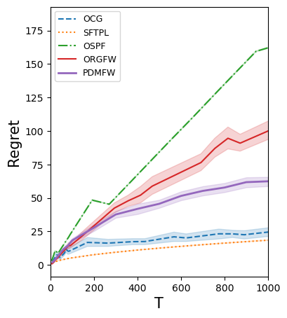
(a)

(b)

Figure 1: Results from testing Algorithms 1 and 2 on matrix completion instances

Figure 1 shows the regret values of the algorithms. PDMFW is Algorithm 2 while the others correspond to Algorithm 1 with oracles listed in Table 2. Note that each algorithm exhibits a sublinear growth in regret, as expected from our theoretical results. In particular, Algorithm 1 with $\mathsf{OCG}$ and Algorithm 1 with $\mathsf{SFTPL}$ achieve lower regret values than the others. Figure 1 summarizes the constraint violations of the algorithms. We observe that constraint violation values are centered around 0. In fact, there exists some instances where the constraint violation is below 0. This is possible because the benchmark $\bm{x^{*}}$ is set to a solution with $\bar{g}(\bm{x^{*}})\leq 0$. Nevertheless, the results shown in Figure 1 support the theoretical results that Algorithms 1 and 2 attain sublinear constraint violations.

Acknowledgements

This research is supported, in part, by the KAIST Starting Fund (KAIST-G04220016), the FOUR Brain Korea 21 Program (NRF-5199990113928), the National Research Foundation of Korea (NRF-2022M3J6A1063021).

Appendix A Performance Analysis of Online Primal-Dual Projection-Free Framework (Algorithm 1)

Let us define filtration $\{\mathcal{F}_{t}:\ t\geq 0\}$ where $\mathcal{F}_{0}=\{\emptyset,\Omega\}$ and $\mathcal{F}_{t}=\sigma(\bm{\omega_{1}},\ldots,\bm{\omega_{t}})$ being the $\sigma$-algebra generated by the set of random samples $\{\bm{\omega_{1}},\ldots,\bm{\omega_{t}}\}$. Note that $\bm{x_{t}}$ is $\mathcal{F}_{t-1}$-measurable for all $t\geq 1$.

For simplicity, we define vector $\bm{x_{k}^{q}}$ and functions $f_{k}^{q},g_{k}^{q},h_{k}^{q},L_{k}^{q}$ for $q\in[Q]$ and $k\in[K]$ as

$$\bm{x_{k}^{q}}=\bm{x_{t}},\quad f_{k}^{q}(\bm{x})=f_{t}(\bm{x}),\quad g_{k}^{q}(\bm{x})=g_{t}(\bm{x}),\quad h_{k}^{q}(\bm{x})=h_{t}(\bm{x}),\quad L_{k}^{q}(\bm{x})=L_{t}(\bm{x},\lambda)$$

for any $\bm{x}\in\mathcal{X}$ and $\lambda\geq 0$ where $t=k+(q-1)K.$ Then it follows that

$$h_{k}^{q}(\bm{x}) =f_{k}^{q}(\bm{x})+\lambda_{q}g_{k}^{q}(\bm{x}),$$

$$L_{k}^{q}(\bm{x},\lambda) =f_{k}^{q}(\bm{x})+\lambda_{q}g_{k}^{q}(\bm{x})-\frac{\theta}{2K}\lambda^{2}$$

$$=h_{k}^{q}(\bm{x})-\frac{\theta}{2K}\lambda^{2}.$$

Moreover, note that

$$\begin{aligned} \sum_{t=(q-1)K+1}^{qK}\left(L_{t}(\bm{x_{t}},\lambda_{q})-L_{t}(\bm{x},\lambda_{q})\right)&=\sum_{k=1}^{K}\left(L_{k}^{q}(\bm{x_{k}^{q}},\lambda_{q})-L_{k}^{q}(\bm{x},\lambda_{q})\right)\\ &=\sum_{k=1}^{K}\left(h_{k}^{q}(\bm{x_{k}^{q}})-h_{k}^{q}(\bm{x})\right)\end{aligned}$$ (8)

Lemma A.1.

Let $\bm{x_{k}^{q}}$ for $k=1,\ldots,K$ be decisions determined by an $(\alpha,C_{0},C_{1},C_{2})$-oracle. Then

$$\mathbb{E}\left[\sum_{k=1}^{K}\left(h_{k}^{q}(\bm{x_{k}^{q}})-h_{k}^{q}(\bm{x})\right)\mid\mathcal{F}_{(q-1)K}\right]\leq(C_{0}+C_{1}D(1+\lambda_{q})+C_{2}L(1+\lambda_{q}))T^{\frac{\alpha}{3-2\alpha}}$$

for any $\bm{x}\in\mathcal{X}$.

Proof.

As we assumed that the loss functions $f_{1},\ldots,f_{T}$ and the constraint functions $g_{1},\ldots,g_{T}$ are $D$-Lipschitz and $L$-smooth, it follows that $h_{1},\ldots,h_{T}$ are $D(1+\lambda_{q})$-Lipschitz and $L(1+\lambda_{q})$-smooth. Then

$$\mathbb{E}\left[\sum_{k=1}^{K}\left(h_{k}^{q}(\bm{x_{k}^{q}})-h_{k}^{q}(\bm{x})\right)\mid\mathcal{F}_{(q-1)K}\right] \leq\mathbb{E}\left[\sum_{k=1}^{K}\left(h_{k}^{q}(\bm{x_{k}^{q}})-\min_{\bm{x}\in\mathcal{X}}h_{k}^{q}(\bm{x})\right)\mid\mathcal{F}_{(q-1)K}\right]$$

$$\leq(C_{0}+C_{1}D(1+\lambda_{q})+C_{2}L(1+\lambda_{q}))K^{\alpha}.$$

Here, we have $K=T^{\frac{1}{3-2\alpha}}$, as required. ∎

Next, observe that

$$\begin{aligned} \sum_{t=(q-1)K+1}^{qK}\left(L_{t}(\bm{x_{t}},\lambda)-L_{t}(\bm{x_{t}},\lambda_{q})\right)&=\sum_{k=1}^{K}\left(L_{k}^{q}(\bm{x_{k}^{q}},\lambda)-L_{k}^{q}(\bm{x_{k}^{q}},\lambda_{q})\right).\end{aligned}$$ (9)

Lemma A.2.

Let $\lambda_{1},\ldots,\lambda_{Q}$ be the dual variables chosen by Algorithm 1. Then for any $\lambda\geq 0$,

$$\sum_{q=1}^{Q}\sum_{k=1}^{K}\left(L_{k}^{q}(\bm{x_{k}^{q}},\lambda)-L_{k}^{q}(\bm{x_{k}^{q}},\lambda_{q})\right)\leq\frac{1}{2\mu}\lambda^{2}+G^{2}K^{2}Q\mu+\theta^{2}\mu\sum_{q=1}^{Q}\lambda_{q}^{2}.$$

Proof.

Note that

$$\lambda_{q+1}=\left[\lambda_{q}+\mu\sum_{k=1}^{K}\nabla_{\lambda}L_{k}^{q}(\bm{x_{k}^{q}},\lambda_{q})\right]_{+}.$$

Then

$$\left(\lambda_{q+1}-\lambda\right)^{2} \leq\left(\lambda_{q}+\mu\sum_{k=1}^{K}\nabla_{\lambda}L_{k}^{q}(\bm{x_{k}^{q}},\lambda_{q})-\lambda\right)^{2}$$

$$=\left(\lambda_{q}-\lambda\right)^{2}+\mu^{2}\left(\sum_{k=1}^{K}g_{k}^{q}(\bm{x_{k}^{q}})-\theta\lambda_{q}\right)^{2}+2\mu\left(\sum_{k=1}^{K}\nabla_{\lambda}L_{k}^{q}(\bm{x_{k}^{q}},\lambda_{q})\right)^{\top}(\lambda_{q}-\lambda)$$

$$\leq\left(\lambda_{q}-\lambda\right)^{2}+2\mu^{2}(G^{2}K^{2}+\theta^{2}\lambda_{q}^{2})+2\mu\sum_{k=1}^{K}\left(L_{k}^{q}(\bm{x_{k}^{q}},\lambda_{q})-L_{k}^{q}(\bm{x_{k}^{q}},\lambda)\right).$$

Therefore, it follows that

$$\sum_{q=1}^{Q}\sum_{k=1}^{K}\left(L_{k}^{q}(\bm{x_{k}^{q}},\lambda_{q})-L_{k}^{q}(\bm{x_{k}^{q}},\lambda)\right)$$

$$\leq\sum_{q=1}^{Q}\frac{1}{2\mu}\left((\lambda_{q}-\lambda)^{2}-(\lambda_{q+1}-\lambda)^{2}\right)+G^{2}K^{2}Q\mu+\theta^{2}\mu\sum_{q=1}^{Q}\lambda_{q}^{2}$$

$$=\frac{1}{2\mu}\lambda^{2}-\frac{1}{2\mu}(\lambda_{Q+1}-\lambda)^{2}+G^{2}K^{2}Q\mu+\theta^{2}\mu\sum_{q=1}^{Q}\lambda_{q}^{2}$$

$$\leq\frac{1}{2\mu}\lambda^{2}+G^{2}K^{2}Q\mu+\theta^{2}\mu\sum_{q=1}^{Q}\lambda_{q}^{2}$$

where the last inequality holds because $(\lambda_{Q+1}-\lambda)^{2}\geq 0$. ∎

Note that

$$\begin{aligned} &\sum_{q=1}^{Q}\sum_{t=(q-1)K+1}^{qK}\left(L_{t}(\bm{x_{t}},\lambda)-L_{t}(\bm{x},\lambda_{q})\right)\\ &=\sum_{q=1}^{Q}\sum_{k=1}^{K}\left(L_{k}^{q}(\bm{x_{k}^{q}},\lambda)-L_{k}^{q}(\bm{x},\lambda_{q})\right)\\ &=\sum_{q=1}^{Q}\sum_{k=1}^{K}\left(f_{k}^{q}(\bm{x_{k}^{q}})-f_{k}^{q}(\bm{x})\right)+\lambda\sum_{q=1}^{Q}\sum_{k=1}^{K}g_{k}^{q}(\bm{x_{k}^{q}})-\sum_{q=1}^{Q}\lambda_{q}\sum_{k=1}^{K}g_{k}^{q}(\bm{x})-\frac{Q\theta}{2}\lambda^{2}+\frac{\theta}{2}\sum_{q=1}^{Q}\lambda_{q}^{2}.\end{aligned}$$ (10)

Based on (8), (9), (10), Lemmas A.1 and A.2, we deduce the following lemma.

Lemma A.3.

Let $\bm{x_{k}^{q}}$ for $k=1,\ldots,K$ and $\lambda_{1},\ldots,\lambda_{Q}$ be the decisions and the dual variable chosen by Algorithm 1. Then for any $\bm{x}\in\mathcal{X}$ and $\lambda\geq 0$,

$$\mathbb{E}\left[\sum_{q=1}^{Q}\sum_{k=1}^{K}\left(f_{k}^{q}(\bm{x_{k}^{q}})-f_{k}^{q}(\bm{x})\right)+\lambda\sum_{q=1}^{Q}\sum_{k=1}^{K}g_{k}^{q}(\bm{x_{k}^{q}})-\sum_{q=1}^{Q}\lambda_{q}\sum_{k=1}^{K}g_{k}^{q}(\bm{x})\right]$$

$$\leq\frac{1}{2}\left(\frac{1}{\mu}+Q\theta\right)\lambda^{2}+G^{2}K^{2}Q\mu+Q(C_{0}+C_{1}D+C_{2}L)T^{\frac{\alpha}{3-2\alpha}}+\frac{Q}{2}(C_{1}D+C_{2}L)T^{\frac{\alpha}{3-2\alpha}+\beta}.$$

Proof.

Note that

$$\sum_{q=1}^{Q}\sum_{k=1}^{K}\left(f_{k}^{q}(\bm{x_{k}^{q}})-f_{k}^{q}(\bm{x})\right)+\lambda\sum_{q=1}^{Q}\sum_{k=1}^{K}g_{k}^{q}(\bm{x_{k}^{q}})-\sum_{q=1}^{Q}\lambda_{q}\sum_{k=1}^{K}g_{k}^{q}(\bm{x})$$

$$=\sum_{q=1}^{Q}\sum_{k=1}^{K}\left(L_{k}^{q}(\bm{x_{k}^{q}},\lambda)-L_{k}^{q}(\bm{x},\lambda_{q})\right)+\frac{Q\theta}{2}\lambda^{2}-\frac{\theta}{2}\sum_{q=1}^{Q}\lambda_{q}^{2}$$

$$=\sum_{q=1}^{Q}\sum_{k=1}^{K}\left(h_{k}^{q}(\bm{x_{k}^{q}})-h_{k}^{q}(\bm{x})\right)+\sum_{q=1}^{Q}\sum_{k=1}^{K}\left(L_{k}^{q}(\bm{x_{k}^{q}},\lambda)-L_{k}^{q}(\bm{x_{k}^{q}},\lambda_{q})\right)+\frac{Q\theta}{2}\lambda^{2}-\frac{\theta}{2}\sum_{q=1}^{Q}\lambda_{q}^{2}$$

$$\leq\sum_{q=1}^{Q}\sum_{k=1}^{K}\left(h_{k}^{q}(\bm{x_{k}^{q}})-h_{k}^{q}(\bm{x})\right)+\frac{1}{2}\left(\frac{1}{\mu}+Q\theta\right)\lambda^{2}+G^{2}K^{2}Q\mu+\left(\theta^{2}\mu-\frac{\theta}{2}\right)\sum_{q=1}^{Q}\lambda_{q}^{2}$$

where the first equality is from (10), the second equality is due to (8) and (9), and the last inequality follows from Lemma A.2. By Lemma A.1,

$$\mathbb{E}\left[\sum_{q=1}^{Q}\sum_{k=1}^{K}\left(h_{k}^{q}(\bm{x_{k}^{q}})-h_{k}^{q}(\bm{x})\right)\right] =\sum_{q=1}^{Q}\mathbb{E}\left[\mathbb{E}\left[\sum_{k=1}^{K}\left(h_{k}^{q}(\bm{x_{k}^{q}})-h_{k}^{q}(\bm{x})\right)\mid\mathcal{F}_{(q-1)K}\right]\right]$$

$$\leq\sum_{q=1}^{Q}\mathbb{E}\left[(C_{0}+C_{1}D(1+\lambda_{q})+C_{2}L(1+\lambda_{q}))T^{\frac{\alpha}{3-2\alpha}}\right].$$

Here, using the fact that $a+b\geq 2\sqrt{ab}$ for any $a,b\geq 0$, we obtain

$$\lambda_{q}T^{\frac{\alpha}{3-2\alpha}}\leq\frac{1}{2}T^{\frac{\alpha}{3-2\alpha}+\beta}+\frac{\lambda_{q}^{2}}{2}T^{\frac{\alpha}{3-2\alpha}-\beta}.$$

Therefore, it follows that

$$\sum_{q=1}^{Q}(C_{0}+C_{1}D(1+\lambda_{q})+C_{2}L(1+\lambda_{q}))T^{\frac{\alpha}{3-2\alpha}}$$

$$\leq Q(C_{0}+C_{1}D+C_{2}L)T^{\frac{\alpha}{3-2\alpha}}+\frac{Q}{2}(C_{1}D+C_{2}L)T^{\frac{\alpha}{3-2\alpha}+\beta}+\frac{1}{2}(C_{1}D+C_{2}L)T^{\frac{\alpha}{3-2\alpha}-\beta}\sum_{q=1}^{Q}\lambda_{q}^{2}$$

$$=Q(C_{0}+C_{1}D+C_{2}L)T^{\frac{\alpha}{3-2\alpha}}+\frac{Q}{2}(C_{1}D+C_{2}L)T^{\frac{\alpha}{3-2\alpha}+\beta}+\frac{\theta}{6}\sum_{q=1}^{Q}\lambda_{q}^{2}.$$

Note that

$$\left(\theta^{2}\mu-\frac{\theta}{2}\right)\sum_{q=1}^{Q}\lambda_{q}^{2}+\frac{\theta}{6}\sum_{q=1}^{Q}\lambda_{q}^{2}=\left(\theta^{2}\mu-\frac{\theta}{3}\right)\sum_{q=1}^{Q}\lambda_{q}^{2}=\left(\frac{\theta}{Q+1}-\frac{\theta}{3}\right)\sum_{q=1}^{Q}\lambda_{q}^{2}.$$

Since $\lambda_{1}=0$ and $Q+1\geq 3$ for $Q\geq 2$, we have

$$\left(\frac{\theta}{Q+1}-\frac{\theta}{3}\right)\sum_{q=1}^{Q}\lambda_{q}^{2}\leq 0,$$

as required. ∎

Proof of Theorem 1.

By plugging in (3) to the inequality given in Lemma A.3, it follows that

$$\mathbb{E}\left[\sum_{q=1}^{Q}\sum_{k=1}^{K}\left(f_{k}^{q}(\bm{x_{k}^{q}})-f_{k}^{q}(\bm{x})\right)+\lambda\sum_{q=1}^{Q}\sum_{k=1}^{K}g_{k}^{q}(\bm{x_{k}^{q}})-\sum_{q=1}^{Q}\lambda_{q}\sum_{k=1}^{K}g_{k}^{q}(\bm{x})\right]$$

$$\leq\frac{1}{2}\left(\frac{1}{\mu}+Q\theta\right)\lambda^{2}+G^{2}K^{2}Q\mu+Q(C_{0}+C_{1}D+C_{2}L)T^{\frac{\alpha}{3-2\alpha}}+\frac{Q}{2}(C_{1}D+C_{2}L)T^{\frac{\alpha}{3-2\alpha}+\beta}$$

$$=\frac{1}{2}(2Q+1)\theta\lambda^{2}+\frac{G^{2}K^{2}Q}{\theta(Q+1)}+Q(C_{0}+C_{1}D+C_{2}L)T^{\frac{\alpha}{3-2\alpha}}+\frac{Q}{2}(C_{1}D+C_{2}L)T^{\frac{\alpha}{3-2\alpha}+\beta}$$

$$\leq 2Q\theta\lambda^{2}+\frac{G^{2}K^{2}}{\theta}+Q(C_{0}+C_{1}D+C_{2}L)T^{\frac{\alpha}{3-2\alpha}}+\frac{Q}{2}(C_{1}D+C_{2}L)T^{\frac{\alpha}{3-2\alpha}+\beta}$$

$$=6(C_{1}D+C_{2}L)T^{\frac{2-\alpha}{3-2\alpha}-\beta}\lambda^{2}+\frac{G^{2}}{3(C_{1}D+C_{2}L)}T^{\frac{2-\alpha}{3-2\alpha}+\beta}$$

$$\quad+(C_{0}+C_{1}D+C_{2}L)T^{\frac{2-\alpha}{3-2\alpha}}+\frac{1}{2}(C_{1}D+C_{2}L)T^{\frac{2-\alpha}{3-2\alpha}+\beta}$$

$$\leq 6(C_{1}D+C_{2}L)T^{\frac{2-\alpha}{3-2\alpha}-\beta}\lambda^{2}+\left(\frac{G^{2}}{3(C_{1}D+C_{2}L)}+\frac{3(C_{0}+C_{1}D+C_{2}L)}{2}\right)T^{\frac{2-\alpha}{3-2\alpha}+\beta}.$$

Moreover, as $\bar{g}(\bm{x^{*}})\leq 0$,

$$\mathbb{E}\left[\sum_{q=1}^{Q}\lambda_{q}\sum_{k=1}^{K}g_{k}^{q}(\bm{x^{*}})\right] =\sum_{q=1}^{Q}\mathbb{E}\left[\mathbb{E}\left[\lambda_{q}\sum_{k=1}^{K}g_{k}^{q}(\bm{x^{*}})\mid\mathcal{F}_{(q-1)K}\right]\right]$$

$$=\sum_{q=1}^{Q}\mathbb{E}\left[\lambda_{q}\sum_{k=1}^{K}\mathbb{E}\left[g_{k}^{q}(\bm{x^{*}})\mid\mathcal{F}_{(q-1)K}\right]\right]$$

$$=\sum_{q=1}^{Q}\mathbb{E}\left[\lambda_{q}\sum_{k=1}^{K}\bar{g}(\bm{x^{*}})\right]$$

$$\leq 0.$$

This implies that

$$\mathbb{E}\left[\sum_{q=1}^{Q}\sum_{k=1}^{K}\left(f_{k}^{q}(\bm{x_{k}^{q}})-f_{k}^{q}(\bm{x^{*}})\right)+\lambda\sum_{q=1}^{Q}\sum_{k=1}^{K}g_{k}^{q}(\bm{x_{k}^{q}})\right]$$

$$\leq 6(C_{1}D+C_{2}L)T^{\frac{2-\alpha}{3-2\alpha}-\beta}\lambda^{2}+\left(\frac{G^{2}}{3(C_{1}D+C_{2}L)}+\frac{3(C_{0}+C_{1}D+C_{2}L)}{2}\right)T^{\frac{2-\alpha}{3-2\alpha}+\beta}.$$

Next, we set

$$\lambda=\frac{1}{12(C_{1}D+C_{2}L)T^{\frac{2-\alpha}{3-2\alpha}-\beta}}\left[\mathbb{E}\left[\sum_{q=1}^{Q}\sum_{k=1}^{K}g_{k}^{q}(\bm{x_{k}^{q}})\right]\right]_{+}.$$

Then we obtain

$$\mathbb{E}\left[\sum_{q=1}^{Q}\sum_{k=1}^{K}\left(f_{k}^{q}(\bm{x_{k}^{q}})-f_{k}^{q}(\bm{x^{*}})\right)\right] \leq-\frac{1}{24(C_{1}D+C_{2}L)T^{\frac{2-\alpha}{3-2\alpha}-\beta}}\left[\mathbb{E}\left[\sum_{q=1}^{Q}\sum_{k=1}^{K}g_{k}^{q}(\bm{x_{k}^{q}})\right]\right]_{+}^{2}$$

$$\quad+\left(\frac{G^{2}}{3(C_{1}D+C_{2}L)}+\frac{3(C_{0}+C_{1}D+C_{2}L)}{2}\right)T^{\frac{2-\alpha}{3-2\alpha}+\beta}.$$

As a result,

$$\mathbb{E}\left[\sum_{q=1}^{Q}\sum_{k=1}^{K}\left(f_{k}^{q}(\bm{x_{k}^{q}})-f_{k}^{q}(\bm{x^{*}})\right)\right] \leq\left(\frac{G^{2}}{3(C_{1}D+C_{2}L)}+\frac{3(C_{0}+C_{1}D+C_{2}L)}{2}\right)T^{\frac{2-\alpha}{3-2\alpha}+\beta}.$$

Moreover,

$$\frac{1}{24(C_{1}D+C_{2}L)T^{\frac{2-\alpha}{3-2\alpha}-\beta}}\left[\mathbb{E}\left[\sum_{q=1}^{Q}\sum_{k=1}^{K}g_{k}^{q}(\bm{x_{k}^{q}})\right]\right]_{+}^{2}$$

$$\leq-\mathbb{E}\left[\sum_{q=1}^{Q}\sum_{k=1}^{K}\left(f_{k}^{q}(\bm{x_{k}^{q}})-f_{k}^{q}(\bm{x^{*}})\right)\right]+\left(\frac{G^{2}}{3(C_{1}D+C_{2}L)}+\frac{3(C_{0}+C_{1}D+C_{2}L)}{2}\right)T^{\frac{2-\alpha}{3-2\alpha}+\beta}$$

$$\leq TDR+\left(\frac{G^{2}}{3(C_{1}D+C_{2}L)}+\frac{3(C_{0}+C_{1}D+C_{2}L)}{2}\right)T^{\frac{2-\alpha}{3-2\alpha}+\beta}$$

where the second inequality holds because $f_{1},\ldots,f_{T}$ are $D$-Lipschitz. Then

$$\mathbb{E}\left[\sum_{q=1}^{Q}\sum_{k=1}^{K}g_{k}^{q}(\bm{x_{k}^{q}})\right]$$

$$\leq\left[\mathbb{E}\left[\sum_{q=1}^{Q}\sum_{k=1}^{K}g_{k}^{q}(\bm{x_{k}^{q}})\right]\right]_{+}$$

$$\leq\sqrt{24(C_{1}D+C_{2}L)T^{\frac{2-\alpha}{3-2\alpha}-\beta}\left(TDR+\left(\frac{G^{2}}{3(C_{1}D+C_{2}L)}+\frac{3(C_{0}+C_{1}D+C_{2}L)}{2}\right)T^{\frac{2-\alpha}{3-2\alpha}+\beta}\right)}$$

$$=O\left(T^{\frac{5-3\alpha}{6-4\alpha}-\frac{\beta}{2}}\right).$$

Then the result follows as

$$\mathbb{E}\left[\sum_{t=1}^{T}\left(f_{t}(\bm{x_{t}})-f_{t}(\bm{x^{*}})\right)\right] =\mathbb{E}\left[\sum_{q=1}^{Q}\sum_{k=1}^{K}\left(f_{k}^{q}(\bm{x_{k}^{q}})-f_{k}^{q}(\bm{x^{*}})\right)\right],$$

$$\mathbb{E}\left[\sum_{t=1}^{T}g_{t}(\bm{x_{t}})\right] =\mathbb{E}\left[\sum_{q=1}^{Q}\sum_{k=1}^{K}g_{k}^{q}(\bm{x_{k}^{q}})\right],$$

as required. ∎

Appendix B Performance Analysis of PMFWG (Algorithm 2)

We provide the proof of Lemma 5.1 in Section B.1. Then, in Section B.2 we show Theorem 2.

B.1 Regret of FTPL: Proof of Lemma 5.1

Recall that our adaptive variant of Follow-The-Perturbed-Leader proceeds as the following setup:

• Choose a random perturbation vector $\bm{p}$ from $[0,1/\delta]^{d}$ for some $\delta>0$ uniformly at random.

• For $t=1,\ldots,T$:

  • Choose

    $$\bm{x_{t}}\in\operatorname*{argmin}_{\bm{x}\in\mathcal{X}}\left(\bm{p}+\sum_{s=1}^{t-1}\bm{w_{s}}\right)^{\top}\bm{x}.$$

  • Observe $\bm{w_{t}}$.

Define $M(\bm{w})=\operatorname*{argmin}_{\bm{x}\in\mathcal{X}}\bm{w}^{\top}\bm{x}$ for $\bm{w}\in\mathbb{R}^{d}$.

Lemma B.1.

The sequence $\{\bm{w_{t}}\}_{t\in[T]}$ satisfies the following.

$$\sum_{t=1}^{T}M\left(\sum_{s=1}^{t}\bm{w_{s}}\right)^{\top}\bm{w_{t}}\leq\sum_{t=1}^{T}M\left(\sum_{s=1}^{T}\bm{w_{s}}\right)^{\top}\bm{w_{t}}.$$

Proof.

We proceed by induction. The case $T=1$ is obvious. Now assume it holds for $T\geq 1$, i.e.,

$$\sum_{t=1}^{T}M\left(\sum_{s=1}^{t}\bm{w_{s}}\right)^{\top}\bm{w_{t}}\leq\sum_{t=1}^{T}M\left(\sum_{s=1}^{T}\bm{w_{s}}\right)^{\top}\bm{w_{t}}.$$

Consider

$$\sum_{t=1}^{T+1}M\left(\sum_{s=1}^{t}\bm{w_{s}}\right)^{\top}\bm{w_{t}} =\sum_{t=1}^{T}M\left(\sum_{s=1}^{t}\bm{w_{s}}\right)^{\top}\bm{w_{t}}+M\left(\sum_{s=1}^{T+1}\bm{w_{s}}\right)^{\top}\bm{w_{T+1}}$$

$$\leq M\left(\sum_{s=1}^{T+1}\bm{w_{s}}\right)^{\top}\bm{w_{T+1}}+\sum_{t=1}^{T}M\left(\sum_{s=1}^{T}\bm{w_{s}}\right)^{\top}\bm{w_{t}}$$

$$=M\left(\sum_{s=1}^{T+1}\bm{w_{s}}\right)^{\top}\bm{w_{T+1}}+M\left(\sum_{s=1}^{T}\bm{w_{s}}\right)^{\top}\left(\sum_{t=1}^{T}\bm{w_{t}}\right)$$

$$\leq M\left(\sum_{s=1}^{T+1}\bm{w_{s}}\right)^{\top}\bm{w_{T+1}}+M\left(\sum_{s=1}^{T}\bm{w_{s}}+\bm{w_{T+1}}\right)^{\top}\left(\sum_{t=1}^{T}\bm{w_{t}}\right)$$

$$=\sum_{t=1}^{T+1}M\left(\sum_{s=1}^{T+1}\bm{w_{s}}\right)^{\top}\bm{w_{t}}$$

where the first inequality comes from the induction hypothesis and the second inequality is because of the definition of $M(\cdot)$, as required. ∎

Lemma B.2.

Define $\bm{p_{0}}:=\bm{0}$. Then for any sequence $\bm{p_{1}},\ldots,\bm{p_{T}}$ we have

$$\sum_{t=1}^{T}M\left(\bm{p_{t}}+\sum_{s=1}^{t}\bm{w_{s}}\right)^{\top}\bm{w_{t}}\leq\sum_{t=1}^{T}M\left(\sum_{s=1}^{T}\bm{w_{s}}\right)^{\top}\bm{w_{t}}+R\sum_{t=1}^{T}\|\bm{p_{t}}-\bm{p_{t-1}}\|_{\infty}.$$

Consequently, if $\bm{p_{t}}=\bm{p}$ for all $t\in[T]$, we have

$$\sum_{t=1}^{T}M\left(\bm{p}+\sum_{s=1}^{t}\bm{w_{s}}\right)^{\top}\bm{w_{t}}\leq\sum_{t=1}^{T}M\left(\sum_{s=1}^{T}\bm{w_{s}}\right)^{\top}\bm{w_{t}}+R\|\bm{p}\|_{\infty}.$$

Proof.

We invoke Lemma B.1 with $\bm{w_{t}^{\prime}}=\bm{w_{t}}+\bm{p_{t}}-\bm{p_{t-1}}$ to obtain

$$\sum_{t=1}^{T}M\left(\bm{p_{t}}+\sum_{s=1}^{t}\bm{w_{s}}\right)^{\top}(\bm{w_{t}}+\bm{p_{t}}-\bm{p_{t-1}})$$

$$\leq\sum_{t=1}^{T}M\left(\bm{p_{T}}+\sum_{s=1}^{T}\bm{w_{s}}\right)^{\top}(\bm{w_{t}}+\bm{p_{t}}-\bm{p_{t-1}})$$

$$=M\left(\bm{p_{T}}+\sum_{s=1}^{T}\bm{w_{s}}\right)^{\top}\left(\bm{p_{T}}+\sum_{t=1}^{T}\bm{w_{t}}\right)$$

$$\leq M\left(\sum_{s=1}^{T}\bm{w_{s}}\right)^{\top}\left(\bm{p_{T}}+\sum_{t=1}^{T}\bm{w_{t}}\right)$$

$$=M\left(\sum_{s=1}^{T}\bm{w_{s}}\right)^{\top}\left(\sum_{t=1}^{T}\bm{w_{t}}\right)+M\left(\sum_{s=1}^{T}\bm{w_{s}}\right)^{\top}\left(\sum_{t=1}^{T}(\bm{p_{t}}-\bm{p_{t-1}})\right)$$

where the second inequality follows from the definition of $M(\cdot)$. This inequality implies that

$$\sum_{t=1}^{T}M\left(\bm{p_{t}}+\sum_{s=1}^{t}\bm{w_{s}}\right)^{\top}\bm{w_{t}}$$

$$\leq M\left(\sum_{s=1}^{T}\bm{w_{s}}\right)^{\top}\left(\sum_{t=1}^{T}\bm{w_{t}}\right)+\sum_{t=1}^{T}\left(M\left(\sum_{s=1}^{T}\bm{w_{s}}\right)-M\left(\bm{p_{t}}+\sum_{s=1}^{t}\bm{w_{s}}\right)\right)^{\top}\left(\bm{p_{t}}-\bm{p_{t-1}}\right)$$

$$\leq M\left(\sum_{s=1}^{T}\bm{w_{s}}\right)^{\top}\left(\sum_{t=1}^{T}\bm{w_{t}}\right)+R\sum_{t=1}^{T}\|\bm{p_{t}}-\bm{p_{t-1}}\|_{\infty},$$

as required. ∎

Lemma B.3.

Let $\bm{p}$ be a vector sampled from $[0,1/\delta]^{n}$ uniformly at random, and $\bm{w},\bm{w^{\prime}},\bm{w^{\prime\prime}}$ be three arbitrary fixed vectors. Then

$$\mathbb{E}\left[\left(M(\bm{w}+\bm{p})-M(\bm{w}+\bm{w^{\prime}}+\bm{p})\right)^{\top}\bm{w^{\prime\prime}}\right]\leq R\|\bm{w^{\prime\prime}}\|_{\infty}\sum_{i=1}^{d}\min\left\{1,\delta|w_{i}^{\prime}|\right\}.$$

Proof.

We consider the hypercubes $C=\bm{w}+[0,1/\delta]^{d}$, $C^{\prime}=\bm{w}+\bm{w^{\prime}}+[0,1/\delta]^{d}$. Note that $\bm{\tilde{p}}:=\bm{w}+\bm{p}$ is uniformly distributed over $C$ and $\bm{\tilde{p}^{\prime}}:=\bm{w}+\bm{w^{\prime}}+\bm{p}$ is uniformly distributed over $C^{\prime}$. Let $C_{\cap}=C\cap C^{\prime}$ and $C_{\circ}=(C\cup C^{\prime})\setminus(C\cap C^{\prime})$. Now

$$\mathbb{E}\left[\left(M(\bm{\tilde{p}})-M(\bm{\tilde{p}^{\prime}})\right)^{\top}\bm{w^{\prime\prime}}\right]$$

$$=\mathbb{E}\left[M(\bm{\tilde{p}})^{\top}\bm{w^{\prime\prime}}\mid\bm{\tilde{p}}\in C_{\cap}\right]\mathbb{P}[\bm{\tilde{p}}\in C_{\cap}]+\mathbb{E}\left[M(\bm{\tilde{p}})^{\top}\bm{w^{\prime\prime}}\mid\bm{\tilde{p}}\in C_{\circ}\right]\mathbb{P}[\bm{\tilde{p}}\in C_{\circ}]$$

$$\quad-\mathbb{E}\left[M(\bm{\tilde{p}^{\prime}})^{\top}\bm{w^{\prime\prime}}\mid\bm{\tilde{p}^{\prime}}\in C_{\cap}\right]\mathbb{P}[\bm{\tilde{p}^{\prime}}\in C_{\cap}]-\mathbb{E}\left[M(\bm{\tilde{p}^{\prime}})^{\top}\bm{w^{\prime\prime}}\mid\bm{\tilde{p}^{\prime}}\in C_{\circ}\right]\mathbb{P}[\bm{\tilde{p}^{\prime}}\in C_{\circ}].$$

Since $\bm{p}$ is uniform on the hypercube, the distribution of $\bm{\tilde{p}}\mid\bm{\tilde{p}}\in C_{\cap}$ is equal to the distribution of $\bm{\tilde{p}^{\prime}}\mid\bm{\tilde{p}^{\prime}}\in C_{\cap}$, and also the probability that each vector is in $C_{\cap}$ is equal. Therefore,

$$\mathbb{E}\left[\left(M(\bm{\tilde{p}})-M(\bm{\tilde{p}^{\prime}})\right)^{\top}\bm{w^{\prime\prime}}\right]$$

$$=\mathbb{E}\left[M(\bm{\tilde{p}})^{\top}\bm{w^{\prime\prime}}\mid\bm{\tilde{p}}\in C_{\circ}\right]\mathbb{P}[\bm{\tilde{p}}\in C_{\circ}]-\mathbb{E}\left[M(\bm{\tilde{p}^{\prime}})^{\top}\bm{w^{\prime\prime}}\mid\bm{\tilde{p}^{\prime}}\in C_{\circ}\right]\mathbb{P}[\bm{\tilde{p}^{\prime}}\in C_{\circ}].$$

Since $\mathbb{P}[\bm{\tilde{p}}\in C_{\cap}]=\mathbb{P}[\bm{\tilde{p}^{\prime}}\in C_{\cap}]$ we have $\mathbb{P}[\bm{\tilde{p}}\in C_{\circ}]=\mathbb{P}[\bm{\tilde{p}^{\prime}}\in C_{\circ}]$, hence

$$\mathbb{E}\left[\left(M(\bm{\tilde{p}})-M(\bm{\tilde{p}^{\prime}})\right)^{\top}\bm{w^{\prime\prime}}\right]$$

$$=\mathbb{E}\left[M(\bm{\tilde{p}})^{\top}\bm{w^{\prime\prime}}\mid\bm{\tilde{p}}\in C_{\circ}\right]\mathbb{P}[\bm{\tilde{p}}\in C_{\circ}]-\mathbb{E}\left[M(\bm{\tilde{p}^{\prime}})^{\top}\bm{w^{\prime\prime}}\mid\bm{\tilde{p}}\in C_{\circ}\right]\mathbb{P}[\bm{\tilde{p}^{\prime}}\in C_{\circ}]$$

$$=\mathbb{P}[\bm{\tilde{p}}\in C_{\circ}]\left(\mathbb{E}\left[M(\bm{\tilde{p}})\mid\bm{\tilde{p}}\in C_{\circ}\right]-\mathbb{E}\left[M(\bm{\tilde{p}^{\prime}})\mid\bm{\tilde{p}^{\prime}}\in C_{\circ}\right]\right)^{\top}\bm{w^{\prime\prime}}$$

$$\leq R\|\bm{w^{\prime\prime}}\|_{\infty}\mathbb{P}[\bm{\tilde{p}}\in C_{\circ}].$$

We now estimate $\mathbb{P}[\bm{\tilde{p}}\in C_{\circ}]$. If $\bm{\tilde{p}}\in C\setminus C^{\prime}$ then there exists some $i\in[d]$ such that $\tilde{p}_{i}\in[w_{i},w_{i}+1/\delta]$ but $\tilde{p}_{i}\not\in[w_{i}+w_{i}^{\prime},w_{i}+w_{i}^{\prime}+1/\delta]$. We can compute that

$$\mathbb{P}[\tilde{p}_{i}\in[w_{i},w_{i}+1/\delta]\setminus[w_{i}+w_{i}^{\prime},w_{i}+w_{i}^{\prime}+1/\delta]]=\begin{cases}1,&|w_{i}^{\prime}|\geq 1/\delta\\ \delta{|w_{i}^{\prime}|},&|w_{i}^{\prime}|<1/\delta\end{cases}=\min\left\{1,\delta{|w_{i}^{\prime}|}\right\}.$$

Now observe that

$$\mathbb{P}\left[\bm{\tilde{p}}\in C_{\circ}\right] =\mathbb{P}\left[\bm{\tilde{p}}\in C\setminus C^{\prime}\right]$$

$$=\mathbb{P}\left[\exists i\in[d]\text{ s.t. }\tilde{p}_{i}\in[w_{i},w_{i}+1/\delta]\setminus[w_{i}+w_{i}^{\prime},w_{i}+w_{i}^{\prime}+1/\delta]\right]$$

$$=1-\mathbb{P}\left[\forall i\in[d],\ \tilde{p}_{i}\in[w_{i},w_{i}+1/\delta]\cap[w_{i}+w_{i}^{\prime},w_{i}+w_{i}^{\prime}+1/\delta]\right]$$

$$=1-\prod_{i=1}^{d}\left(1-\mathbb{P}[\tilde{p}_{i}\in[w_{i},w_{i}+1/\delta]\setminus[w_{i}+w_{i}^{\prime},w_{i}+w_{i}^{\prime}+1/\delta]]\right)$$

$$=1-\prod_{i=1}^{d}\left(1-\min\left\{1,\delta{|w_{i}^{\prime}|}\right\}\right)$$

$$=1-\prod_{i=1}^{d}\max\left\{0,1-\delta{|w_{i}^{\prime}|}\right\}$$

$$=\begin{cases}1-\prod_{i=1}^{d}\left(1-\delta{|w_{i}^{\prime}|}\right),&\|\bm{w^{\prime}}\|_{\infty}\leq 1/\delta\\ 1,&\|\bm{w^{\prime}}\|_{\infty}>1/\delta,\end{cases}$$

where the fourth equality follows since each $\tilde{p}_{i}$ is independent. A union bound then gives

$$\mathbb{P}\left[\bm{\bm{\tilde{p}}}\in C_{\circ}\right] =\mathbb{P}\left[\bm{\bm{\tilde{p}}}\in C\setminus C^{\prime}\right]$$

$$=\mathbb{P}\left[\exists i\in[d]\text{ s.t. }\tilde{p}_{i}\in[w_{i},w_{i}+1/\delta]\setminus[w_{i}+w_{i}^{\prime},w_{i}+w_{i}^{\prime}+1/\delta]\right]$$

$$\leq\sum_{i=1}^{d}\mathbb{P}\left[\tilde{p}_{i}\in[w_{i},w_{i}+1/\delta]\setminus[w_{i}+w_{i}^{\prime},w_{i}+w_{i}^{\prime}+1/\delta]\right]$$

$$=\sum_{i=1}^{d}\min\left\{1,\delta{|w_{i}^{\prime}|}\right\},$$

as required. ∎

Theorem 5 (Follow-the-Perturbed-Leader regret bound).

Let $\bm{x_{1}},\ldots,\bm{x_{T}}$ be the sequence of decisions chosen by FTPL for the sequence of linear vectors $\bm{w_{1}},\ldots,\bm{w_{T}}$. Then

$$\mathbb{E}\left[\sum_{t=1}^{T}\bm{w_{t}}^{\top}\bm{x_{t}}\right]-\min_{\bm{x}\in\mathcal{X}}\sum_{t=1}^{T}\bm{w_{t}}^{\top}\bm{x}\leq\frac{R}{\delta}+\delta dR\sum_{t=1}^{T}\|\bm{w_{t}}\|_{\infty}^{2}$$

where the expectation is taken with respect to the randomness of the random perturbation vectors.

Proof.

According to Lemma B.2 we have

$$\sum_{t=1}^{T}M\left(\bm{p}+\sum_{s=1}^{t}\bm{w_{s}}\right)^{\top}\bm{w_{t}} \leq\sum_{t=1}^{T}M\left(\sum_{s=1}^{T}\bm{w_{s}}\right)^{\top}\bm{w_{t}}+R\|\bm{p}\|_{\infty}$$

$$=\min_{\bm{x}\in\mathcal{X}}\sum_{t=1}^{T}\bm{w_{t}}^{\top}\bm{x}+R\|\bm{p}\|_{\infty}$$

$$\leq\min_{\bm{x}\in\mathcal{X}}\sum_{t=1}^{T}\bm{w_{t}}^{\top}\bm{x}+\frac{R}{\delta}$$

where the final inequality follows since $\bm{p}\in[0,1/\delta]^{d}$. Remember that $\bm{x_{t}}=M\left(\bm{p}+\sum_{s=1}^{t-1}\bm{w_{s}}\right)$. Therefore,

$$\sum_{t=1}^{T}\bm{w_{t}}^{\top}\bm{x_{t}} \leq\min_{\bm{x}\in\mathcal{X}}\sum_{t=1}^{T}\bm{w_{t}}^{\top}\bm{x}+\frac{R}{\delta}+\sum_{t=1}^{T}\left(M\left(\bm{p}+\sum_{s=1}^{t-1}\bm{w_{s}}\right)-M\left(\bm{p}+\sum_{s=1}^{t}\bm{w_{s}}\right)\right)^{\top}\bm{w_{t}}.$$

Take expectations of both sides to get

$$\mathbb{E}_{\bm{p}}\left[\sum_{t=1}^{T}\bm{w_{t}}^{\top}\bm{x_{t}}\right]$$

$$\leq\min_{\bm{x}\in\mathcal{X}}\sum_{t=1}^{T}\bm{w_{t}}^{\top}\bm{x}+\frac{R}{\delta}+\sum_{t=1}^{T}\mathbb{E}_{\bm{p}}\left[M\left(\bm{p}+\sum_{s=1}^{t-1}\bm{w_{s}}\right)-M\left(\bm{p}+\sum_{s=1}^{t}\bm{w_{s}}\right)\right]^{\top}\bm{w_{t}}.$$

We now apply Lemma B.3 to each term in the last sum to get

$$\mathbb{E}_{\bm{p}}\left[\sum_{t=1}^{T}\bm{w_{t}}^{\top}\bm{x_{t}}\right]-\min_{\bm{x}\in\mathcal{X}}\sum_{t=1}^{T}\bm{w_{t}}^{\top}\bm{x} \leq\frac{R}{\delta}+\sum_{t=1}^{T}R\|\bm{w_{t}}\|_{\infty}\sum_{i=1}^{d}\min\left\{1,\delta|w_{t,i}|\right\}$$

$$\leq\frac{R}{\delta}+\sum_{t=1}^{T}R\|\bm{w_{t}}\|_{\infty}\sum_{i=1}^{d}\delta|w_{t,i}|$$

$$\leq\frac{R}{\delta}+\delta dR\sum_{t=1}^{T}\|\bm{w_{t}}\|_{\infty}^{2},$$

as required. ∎

Having proved Theorem 5, we can prove Lemma 5.1. Let us define filtration $\{\mathcal{F}_{t}:\ t\geq 0\}$ where $\mathcal{F}_{0}=\{\emptyset,\Omega\}$ and $\mathcal{F}_{t}=\sigma(\bm{\omega_{1}},\ldots,\bm{\omega_{t}})$ being the $\sigma$-algebra generated by the set of random samples $\{\bm{\omega_{1}},\ldots,\bm{\omega_{t}}\}$. Note that $\bm{x_{t}}$ and $\lambda_{t}$ are $\mathcal{F}_{t-1}$-measurable for all $t\geq 1$.

Proof of Lemma 5.1.

Note that the expected regret of FTPL under the sequence of linear functions $h_{1}^{k}(\bm{v}),\ldots,h_{T}^{k}(\bm{v})$ can be bounded using Theorem 5, as follows.

$$\begin{aligned} \mathbb{E}\left[\sum_{t=1}^{T}h_{t}^{k}(\bm{v_{t}^{k}})-\min_{\bm{v}\in\mathcal{X}}\sum_{t=1}^{T}h_{t}^{k}(\bm{v})\right]&=\mathbb{E}\left[\mathbb{E}\left[\sum_{t=1}^{T}h_{t}^{k}(\bm{v_{t}^{k}})\mid\mathcal{F}_{T}\right]-\min_{\bm{v}\in\mathcal{X}}\sum_{t=1}^{T}h_{t}^{k}(\bm{v})\right]\\ &\leq\mathbb{E}\left[\frac{R}{\delta}+\delta dR\sum_{t=1}^{T}\|\nabla f_{t}(\bm{x_{t}^{k}})+\lambda_{t}\nabla g_{t}(\bm{x_{t}^{k}})\|_{\infty}^{2}\right]\\ &\leq\mathbb{E}\left[\frac{R}{\delta}+2\delta dR\sum_{t=1}^{T}\left(\|\nabla f_{t}(\bm{x_{t}^{k}})\|_{\infty}^{2}+\lambda_{t}^{2}\|\nabla g_{t}(\bm{x_{t}^{k}})\|_{\infty}^{2}\right)\right]\end{aligned}$$ (11)

where the first equality holds due to the tower rule, the first inequality follows from Theorem 5, and the second inequality holds because $\|\bm{x}+\bm{y}\|_{\infty}^{2}\leq(\|\bm{x}\|_{\infty}+\|\bm{y}\|_{\infty})^{2}\leq 2\|\bm{x}\|_{\infty}^{2}+2\|\bm{y}\|_{\infty}^{2}$ for any $\bm{x},\bm{y}\in\mathbb{R}^{d}$. Note that

$$\begin{aligned} &\mathbb{E}\left[\frac{R}{\delta}+2\delta dR\sum_{t=1}^{T}\left(\|\nabla f_{t}(\bm{x_{t}^{k}})\|_{\infty}^{2}+\lambda_{t}^{2}\|\nabla g_{t}(\bm{x_{t}^{k}})\|_{\infty}^{2}\right)\right]\\ &=\frac{R}{\delta}+2\delta dR\sum_{t=1}^{T}\left(\|\nabla f_{t}(\bm{x_{t}^{k}})\|_{\infty}^{2}+\mathbb{E}\left[\lambda_{t}^{2}\|\nabla g_{t}(\bm{x_{t}^{k}})\|_{\infty}^{2}\right]\right)\\ &\leq\frac{R}{\delta}+2\delta dR\sum_{t=1}^{T}\left(D^{2}+D^{2}\mathbb{E}\left[\lambda_{t}^{2}\right]\right)\end{aligned}$$ (12)

where the first inequality follows from 2. Since

$$\delta=\frac{1}{2D\sqrt{d}T^{\frac{1}{2}+\beta}},$$

it follows from (11) that

$$\mathbb{E}\left[\sum_{t=1}^{T}h_{t}^{k}(\bm{v_{t}^{k}})-\min_{\bm{v}\in\mathcal{X}}\sum_{t=1}^{T}h_{t}^{k}(\bm{v})\right] \leq\frac{R}{\delta}+{2R\delta d}\sum_{t=1}^{T}(D^{2}+D^{2}\mathbb{E}\left[\lambda_{t}^{2}\right])$$

$$=RD\sqrt{d}\left(3T^{\frac{1}{2}+\beta}+\frac{1}{T^{\frac{1}{2}+\beta}}\mathbb{E}\left[\sum_{t=1}^{T}\lambda_{t}^{2}\right]\right),$$

as required. ∎

B.2 Regret: Proof of Theorem 2

Lemma B.4.

Let $\gamma_{k}=2/(k+1)$ for $k\geq 1$. Then for any $\ell\leq K+1$,

$$\prod_{k=\ell}^{K}(1-\gamma_{k})\leq\left(\frac{\ell+1}{K+2}\right)^{2}.$$

Proof.

If $\ell=K+1$, then both sides are equal to 1, so the inequality is satisfied. Assume that $\ell\leq K$. Then

$$\prod_{k=\ell}^{K}(1-\gamma_{k})\leq\exp\left(-\sum_{k=\ell}^{K}\frac{2}{k+1}\right)\leq\exp\left(-\int_{x=\ell+1}^{K+2}\frac{2}{x}dx\right)=\left(\frac{\ell+1}{K+2}\right)^{2},$$

as required. ∎

First, we prove the following lemma, which holds because $f_{t}$ and $g_{t}$ are smooth (3). We closely follow the proof of Chen et al. [4, Theorem 1]. We define a constant $C_{3}$ as

$$C_{3}=4RD+5R^{2}L+\frac{R(4D+5RL)^{2}}{4D\sqrt{d}}+3RD\sqrt{d}.$$

Lemma B.5.

Let $\gamma_{k}=2/(k+1)$. Then for any $\bm{x}\in\mathcal{X}$,

$$\mathbb{E}\left[\sum_{t=1}^{T}L_{t}(\bm{x_{t}},\lambda_{t})-\sum_{t=1}^{T}L_{t}(\bm{x},\lambda_{t})\right]\leq C_{3}T^{\frac{1}{2}+\beta}+\frac{2RD\sqrt{d}}{T^{\frac{1}{2}+\beta}}\sum_{t=1}^{T}\mathbb{E}\left[\lambda_{t}^{2}\right].$$

Proof.

Observe first that

$$\sum_{t=1}^{T}L_{t}(\bm{x_{t}},\lambda_{t})-\sum_{t=1}^{T}L_{t}(\bm{x},\lambda_{t})=\sum_{t=1}^{T}\left(f_{t}(\bm{x_{t}})-f_{t}(\bm{x})\right)+\sum_{t=1}^{T}\lambda_{t}\left(g_{t}(\bm{x_{t}})-g_{t}(\bm{x})\right).$$ (13)

Let $t\geq 1$. Note that for any $1\leq k\leq K$,

$$\begin{aligned} &f_{t}(\bm{x_{t}^{k+1}})-f_{t}(\bm{x})\\ &=f_{t}(\bm{x_{t}^{k}}+\gamma_{k}(\bm{v_{t}^{k}}-\bm{x_{t}^{k}}))-f_{t}(\bm{x})\\ &\leq f_{t}(\bm{x_{t}^{k}})-f_{t}(\bm{x})+\gamma_{k}\nabla f_{t}(\bm{x_{t}^{k}})^{\top}(\bm{v_{t}^{k}}-\bm{x_{t}^{k}})+\frac{L\gamma_{k}^{2}R^{2}}{2}\\ &=f_{t}(\bm{x_{t}^{k}})-f_{t}(\bm{x})+\gamma_{k}\nabla f_{t}(\bm{x_{t}^{k}})^{\top}(\bm{x}-\bm{x_{t}^{k}})+\gamma_{k}\nabla f_{t}(\bm{x_{t}^{k}})^{\top}(\bm{v_{t}^{k}}-\bm{x})+\frac{L\gamma_{k}^{2}R^{2}}{2}\\ &\leq(1-\gamma_{k})\left(f_{t}(\bm{x_{t}^{k}})-f_{t}(\bm{x})\right)+\gamma_{k}\nabla f_{t}(\bm{x_{t}^{k}})^{\top}(\bm{v_{t}^{k}}-\bm{x})+\frac{L\gamma_{k}^{2}R^{2}}{2}\end{aligned}$$ (14)

where the first inequality holds because $f_{t}$ is $L$-smooth and $\|\bm{v_{t}^{k}}-\bm{x_{t}^{k}}\|_{1}\leq R$ whereas the second inequality follows from the convexity of $f_{t}$. Then it follows from (14) that

$$\begin{aligned} f_{t}(\bm{x_{t}})-f_{t}(\bm{x})&=f_{t}(\bm{x_{t}^{K+1}})-f_{t}(\bm{x})\\ &\leq\prod_{k=1}^{K}(1-\gamma_{k})\left(f_{t}(\bm{x_{t}^{1}})-f_{t}(\bm{x})\right)\\ &\quad+\sum_{k=1}^{K}\gamma_{k}\left(\nabla f_{t}(\bm{x_{t}^{k}})^{\top}(\bm{v_{t}^{k}}-\bm{x})+\frac{L\gamma_{k}R^{2}}{2}\right)\prod_{j=k+1}^{K}(1-\gamma_{j})\\ &=\prod_{k=1}^{K}(1-\gamma_{k})\left(f_{t}(\bm{x_{t-1}})-f_{t}(\bm{x})\right)\\ &\quad+\sum_{k=1}^{K}\gamma_{k}\left(\nabla f_{t}(\bm{x_{t}^{k}})^{\top}(\bm{v_{t}^{k}}-\bm{x})+\frac{L\gamma_{k}R^{2}}{2}\right)\prod_{j=k+1}^{K}(1-\gamma_{j})\\ &\leq\prod_{k=1}^{K}(1-\gamma_{k})DR\\ &\quad+\sum_{k=1}^{K}\gamma_{k}\left(\nabla f_{t}(\bm{x_{t}^{k}})^{\top}(\bm{v_{t}^{k}}-\bm{x})+\frac{L\gamma_{k}R^{2}}{2}\right)\prod_{j=k+1}^{K}(1-\gamma_{j})\end{aligned}$$ (15)

where the last inequality holds because $f_{t}$ is $D$-Lipschitz. Similarly, we deduce that

$$\begin{aligned} &\mathbb{E}\left[\lambda_{t}\left(g_{t}(\bm{x_{t}})-g_{t}(\bm{x})\right)\right]\\ &\leq\prod_{k=1}^{K}(1-\gamma_{k})DR\mathbb{E}\left[\lambda_{t}\right]\\ &\quad+\sum_{k=1}^{K}\gamma_{k}\left(\mathbb{E}\left[\lambda_{t}\nabla g_{t}(\bm{x_{t}^{k}})^{\top}(\bm{v_{t}^{k}}-\bm{x})\right]+\frac{L\gamma_{k}R^{2}}{2}\mathbb{E}\left[\lambda_{t}\right]\right)\prod_{j=k+1}^{K}(1-\gamma_{j}).\end{aligned}$$ (16)

Summing up (15) and (16) for $t=1,\ldots,T$, we obtain

$$\begin{aligned} &\mathbb{E}\left[\sum_{t=1}^{T}L_{t}(\bm{x_{t}},\lambda_{t})-\sum_{t=1}^{T}L_{t}(\bm{x},\lambda_{t})\right]\\ &\leq\sum_{t=1}^{T}\prod_{k=1}^{K}(1-\gamma_{k})DR\left(1+\mathbb{E}\left[\lambda_{t}\right]\right)\\ &\quad+\sum_{t=1}^{T}\sum_{k=1}^{K}\gamma_{k}\mathbb{E}\left[\left(\nabla f_{t}(\bm{x_{t}^{k}})+\lambda_{t}\nabla g_{t}(\bm{x_{t}^{k}})\right)^{\top}(\bm{v_{t}^{k}}-\bm{x})\right]\prod_{j=k+1}^{K}(1-\gamma_{j})\\ &\quad+\sum_{t=1}^{T}\sum_{k=1}^{K}\frac{L\gamma_{k}^{2}R^{2}}{2}\left(1+\mathbb{E}\left[\lambda_{t}\right]\right)\prod_{j=k+1}^{K}(1-\gamma_{j}).\end{aligned}$$ (17)

Here,

$$\begin{aligned} &\sum_{t=1}^{T}\prod_{k=1}^{K}(1-\gamma_{k})DR\left(1+\mathbb{E}\left[\lambda_{t}\right]\right)+\sum_{t=1}^{T}\sum_{k=1}^{K}\frac{L\gamma_{k}^{2}R^{2}}{2}\left(1+\mathbb{E}\left[\lambda_{t}\right]\right)\prod_{j=k+1}^{K}(1-\gamma_{j})\\ &\leq\sum_{t=1}^{T}\frac{4RD}{(K+2)^{2}}\left(1+\mathbb{E}\left[\lambda_{t}\right]\right)+\sum_{t=1}^{T}\sum_{k=1}^{K}\frac{2R^{2}L}{(k+1)^{2}}\left(\frac{k+2}{K+2}\right)^{2}\left(1+\mathbb{E}\left[\lambda_{t}\right]\right)\\ &\leq\sum_{t=1}^{T}\frac{4RD}{K+2}\left(1+\mathbb{E}\left[\lambda_{t}\right]\right)+\sum_{t=1}^{T}\frac{9R^{2}LK}{2\left(K+2\right)^{2}}\left(1+\mathbb{E}\left[\lambda_{t}\right]\right)\\ &\leq\sum_{t=1}^{T}\frac{4RD}{T^{\frac{1}{2}+\beta}}\left(1+\mathbb{E}\left[\lambda_{t}\right]\right)+\sum_{t=1}^{T}\frac{5R^{2}L}{T^{\frac{1}{2}+\beta}}\left(1+\mathbb{E}\left[\lambda_{t}\right]\right)\end{aligned}$$ (18)

where the first inequality follows from Lemma B.4, the second inequality holds because $K+2\geq 1$ and $2(k+2)\leq 3(k+1)$, and the third inequality is obtained using $K+2\geq T^{\frac{1}{2}+\beta}$ and $K\leq T^{\frac{1}{2}+\beta}$. Furthermore,

$$\begin{aligned} &\sum_{t=1}^{T}\sum_{k=1}^{K}\gamma_{k}\prod_{j=k+1}^{K}(1-\gamma_{j})\mathbb{E}\left[\left(\nabla f_{t}(\bm{x_{t}^{k}})+\lambda_{t}\nabla g_{t}(\bm{x_{t}^{k}})\right)^{\top}(\bm{v_{t}^{k}}-\bm{x})\right]\\ &=\sum_{k=1}^{K}\gamma_{k}\prod_{j=k+1}^{K}(1-\gamma_{j})\sum_{t=1}^{T}\mathbb{E}\left[\left(\nabla f_{t}(\bm{x_{t}^{k}})+\lambda_{t}\nabla g_{t}(\bm{x_{t}^{k}})\right)^{\top}(\bm{v_{t}^{k}}-\bm{x})\right]\\ &=\sum_{k=1}^{K}\gamma_{k}\prod_{j=k+1}^{K}(1-\gamma_{j})\mathbb{E}\left[\sum_{t=1}^{T}h_{t}^{k}(\bm{v_{t}^{k}})-\sum_{t=1}^{T}h_{t}^{k}(\bm{x})\right]\\ &\leq\sum_{k=1}^{K}\gamma_{k}\prod_{j=k+1}^{K}(1-\gamma_{j})\mathcal{R}^{\mathcal{E}}(T)\\ &\leq\sum_{k=1}^{K}\frac{2}{(k+1)}\left(\frac{k+2}{K+2}\right)^{2}\mathcal{R}^{\mathcal{E}}(T)\\ &\leq\sum_{k=1}^{K}\frac{3(k+2)}{(K+2)^{2}}\mathcal{R}^{\mathcal{E}}(T)\\ &\leq\frac{3}{2}\mathcal{R}^{\mathcal{E}}(T)\end{aligned}$$ (19)

where the second inequality is from Lemma B.4. By Lemma 5.1, (17), (18), and (19),

$$\begin{aligned} &\mathbb{E}\left[\sum_{t=1}^{T}L_{t}(\bm{x_{t}},\lambda_{t})-\sum_{t=1}^{T}L_{t}(\bm{x},\lambda_{t})\right]\\ &\leq\sum_{t=1}^{T}\frac{4RD+5R^{2}L}{T^{\frac{1}{2}+\beta}}\left(1+\mathbb{E}\left[\lambda_{t}\right]\right)+RD\sqrt{d}\left(3T^{\frac{1}{2}+\beta}+\frac{1}{T^{\frac{1}{2}+\beta}}\sum_{t=1}^{T}\mathbb{E}[\lambda_{t}^{2}]\right).\end{aligned}$$ (20)

Observe that

$$\frac{4RD+5R^{2}L}{T^{{\frac{1}{2}+\beta}}}\lambda_{t}\leq\frac{RD\sqrt{d}}{T^{\frac{1}{2}+\beta}}\lambda_{t}^{2}+\frac{(4RD+5R^{2}L)^{2}}{4RD\sqrt{d}T^{{\frac{1}{2}+\beta}}}=\frac{RD\sqrt{d}}{T^{\frac{1}{2}+\beta}}\lambda_{t}^{2}+\frac{R(4D+5RL)^{2}}{4D\sqrt{d}T^{{\frac{1}{2}+\beta}}}.$$ (21)

as $2\sqrt{pq}\leq p+q$ for any $p,q\geq 0$. Based on (20) and (21),

$$\mathbb{E}\left[\sum_{t=1}^{T}L_{t}(\bm{x_{t}},\lambda_{t})-\sum_{t=1}^{T}L_{t}(\bm{x},\lambda_{t})\right] \leq\sum_{t=1}^{T}\left(4RD+5R^{2}L+\frac{R(4D+5RL)^{2}}{4D\sqrt{d}}\right)\frac{1}{T^{\frac{1}{2}+\beta}}$$

$$\quad+3RD\sqrt{d}T^{\frac{1}{2}+\beta}+\frac{2RD\sqrt{d}}{T^{\frac{1}{2}+\beta}}\sum_{t=1}^{T}\mathbb{E}\left[\lambda_{t}^{2}\right]$$

$$\leq C_{3}T^{\frac{1}{2}+\beta}+\frac{2RD\sqrt{d}}{T^{\frac{1}{2}+\beta}}\sum_{t=1}^{T}\mathbb{E}\left[\lambda_{t}^{2}\right],$$

as required. ∎

Next, based on the concavity of $L_{t}(\bm{x_{t}},\lambda)$ with respect to $\lambda$, we show the following lemma.

Lemma B.6.

For any $\lambda\geq 0$,

$$\mathbb{E}\left[\sum_{t=1}^{T}L_{t}(\bm{x_{t}},\lambda)-\sum_{t=1}^{T}L_{t}(\bm{x_{t}},\lambda_{t})\right]\leq\frac{1}{2\mu}\lambda^{2}+G^{2}T\mu+\mu\theta^{2}\sum_{t=1}^{T}\mathbb{E}\left[\lambda_{t}^{2}\right].$$

Proof.

Note that

$$\begin{aligned} &(\lambda_{t+1}-\lambda)^{2}\\ &\leq(\lambda_{t}+\mu\nabla_{\lambda}L_{t}(\bm{x_{t}},\lambda_{t})-\lambda)^{2}\\ &=(\lambda_{t}-\lambda)^{2}+\mu^{2}(g_{t}(\bm{x_{t}})-\theta\lambda_{t})^{2}+2\mu\nabla_{\lambda}L_{t}(\bm{x_{t}},\lambda_{t})^{\top}(\lambda_{t}-\lambda)\\ &\leq(\lambda_{t}-\lambda)^{2}+\mu^{2}(g_{t}(\bm{x_{t}})-\theta\lambda_{t})^{2}-2\mu\left(L_{t}(\bm{x_{t}},\lambda)-L_{t}(\bm{x_{t}},\lambda_{t})\right)-{\mu\theta}(\lambda_{t}-\lambda)^{2}\end{aligned}$$ (22)

where the first inequality is because $\lambda_{t+1}$ is the projection of $\lambda_{t}+\mu\nabla_{\lambda}L_{t}(\bm{x_{t}},\lambda_{t})$, the equality is because $\nabla_{\lambda}L_{t}(\bm{x_{t}},\lambda_{t})=g_{t}(\bm{x_{t}})-\theta\lambda_{t}$, the second inequality holds because $L_{t}$ is $\theta$-strongly concave with respect to $\lambda$. Note that

$$\begin{aligned} \mathbb{E}\left[(g_{t}(\bm{x_{t}})-\theta\lambda_{t})^{2}\right]&\leq\mathbb{E}\left[2(g_{t}(\bm{x_{t}}))^{2}+2\theta^{2}\lambda_{t}^{2}\right]\\ &=2\mathbb{E}\left[\mathbb{E}\left[(g_{t}(\bm{x_{t}}))^{2}+2\theta^{2}\lambda_{t}^{2}\mid\mathcal{F}_{t-1}\right]\right]\\ &\leq 2G^{2}+2\theta^{2}\mathbb{E}\left[\lambda_{t}^{2}\right].\end{aligned}$$ (23)

Combining (22) and (23),

$$\begin{aligned} &\mathbb{E}\left[(\lambda_{t+1}-\lambda)^{2}\right]\\ &\leq\mathbb{E}\left[(\lambda_{t}-\lambda)^{2}\right]+\mu^{2}(2G^{2}+2\theta^{2}\lambda_{t}^{2})-\mathbb{E}\left[2\mu\left(L_{t}(\bm{x_{t}},\lambda)-L_{t}(\bm{x_{t}},\lambda_{t})\right)\right]-{\mu\theta}(\lambda_{t}-\lambda)^{2}.\end{aligned}$$ (24)

Then it follows from (24) that

$$\begin{aligned} &\mathbb{E}\left[\sum_{t=1}^{T}L_{t}(\bm{x_{t}},\lambda)-\sum_{t=1}^{T}L_{t}(\bm{x_{t}},\lambda_{t})\right]\\ &\leq\mathbb{E}\left[\sum_{t=1}^{T}\frac{1}{2\mu}\left((\lambda_{t}-\lambda)^{2}-(\lambda_{t+1}-\lambda)^{2}\right)+\sum_{t=1}^{T}{\mu}(G^{2}+\theta^{2}\lambda_{t}^{2})-\sum_{t=1}^{T}\frac{\theta}{2}(\lambda_{t}-\lambda)^{2}\right]\\ &\leq\frac{1}{2\mu}(\lambda_{1}-\lambda)^{2}+G^{2}T\mu+\sum_{t=1}^{T}\mu\theta^{2}\mathbb{E}\left[\lambda_{t}^{2}\right]\\ &=\frac{1}{2\mu}\lambda^{2}+G^{2}T\mu+\sum_{t=1}^{T}\mu\theta^{2}\mathbb{E}\left[\lambda_{t}^{2}\right]\end{aligned}$$

where the last inequality holds due to $\lambda_{1}=0$. Therefore, the assertion of the lemma holds, as required. ∎

Based on Lemmas B.5 and B.6, we show the following lemma. Recall that

$$C_{1}=4RD+5R^{2}L+\frac{R(4D+5RL)^{2}}{4D\sqrt{d}}+3RD\sqrt{d}+\frac{G^{2}}{12RD\sqrt{d}}=C_{3}+\frac{G^{2}}{12RD\sqrt{d}}.$$

Lemma B.7.

Let $\gamma_{k}=2/(k+1)$. Then for any $\bm{x}\in\mathcal{X}$ and $\lambda\geq 0$,

$$\mathbb{E}\left[\left(\sum_{t=1}^{T}f_{t}(\bm{x_{t}})-\sum_{t=1}^{T}f_{t}(\bm{x})\right)+\left(\sum_{t=1}^{T}\lambda g_{t}(\bm{x_{t}})-\sum_{t=1}^{T}\lambda_{t}g_{t}(\bm{x})\right)\right]$$

$$\leq C_{1}T^{\frac{1}{2}+\beta}+24RD\sqrt{d}T^{\frac{1}{2}-\beta}\lambda^{2}.$$

Proof.

Adding the two inequalities proved in Lemmas B.5 and B.6, we obtain

$$\begin{aligned} &\mathbb{E}\left[\sum_{t=1}^{T}L_{t}(\bm{x_{t}},\lambda)-\sum_{t=1}^{T}L_{t}(\bm{x},\lambda_{t})\right]\\ &\leq C_{3}T^{\frac{1}{2}+\beta}+\frac{2RD\sqrt{d}}{T^{\frac{1}{2}+\beta}}\sum_{t=1}^{T}\mathbb{E}\left[\lambda_{t}^{2}\right]+\frac{1}{2\mu}\lambda^{2}+G^{2}T\mu+\sum_{t=1}^{T}\mu\theta^{2}\mathbb{E}\left[\lambda_{t}^{2}\right].\end{aligned}$$ (25)

By (25),

$$\mathbb{E}\left[\left(\sum_{t=1}^{T}f_{t}(\bm{x_{t}})-\sum_{t=1}^{T}f_{t}(\bm{x})\right)+\left(\sum_{t=1}^{T}\lambda g_{t}(\bm{x_{t}})-\sum_{t=1}^{T}\lambda_{t}g_{t}(\bm{x})\right)\right]$$

$$\leq C_{3}T^{\frac{1}{2}+\beta}+G^{2}T\mu+\left(\frac{1}{2}T\theta+\frac{1}{2\mu}\right)\lambda^{2}+\sum_{t=1}^{T}\left(\frac{2RD\sqrt{d}}{T^{\beta}}+\mu\theta^{2}-\frac{\theta}{2}\right)\mathbb{E}\left[\lambda_{t}^{2}\right]$$

$$\leq C_{3}T^{\frac{1}{2}+\beta}+G^{2}T\mu+\left(\frac{1}{2}T\theta+\frac{1}{2\mu}\right)\lambda^{2}$$

$$\leq C_{3}T^{\frac{1}{2}+\beta}+\frac{G^{2}}{12RD\sqrt{d}}T^{\frac{1}{2}+\beta}+24RD\sqrt{d}T^{\frac{1}{2}-\beta}\lambda^{2}$$

$$=C_{1}T^{\frac{1}{2}+\beta}+24RD\sqrt{d}T^{\frac{1}{2}-\beta}\lambda^{2}$$

where the second inequality holds because $\lambda_{1}=0$ and for $T\geq 1$,

$$\frac{2RD\sqrt{d}}{T^{\frac{1}{2}+\beta}}+\mu\theta^{2}-\frac{\theta}{2}=\frac{\theta}{6}+\frac{\theta}{T+2}-\frac{\theta}{2}\leq\frac{\theta}{6}+\frac{\theta}{3}-\frac{\theta}{2}=0,$$

as required. ∎

Lastly, we need the following lemma.

Lemma B.8.

For any $\{\lambda_{t}\}_{t=1}^{T}\subseteq\mathbb{R}_{+}$ such that $\lambda_{t}$ is $\mathcal{F}_{t-1}$-measurable for $t\geq 1$, then

$$\mathbb{E}\left[\sum_{t=1}^{T}\lambda_{t}g_{t}(\bm{x^{*}})\right]\leq 0$$

Proof.

Note that

$$\mathbb{E}[\lambda_{t}g_{t}(\bm{x^{*}})] =\mathbb{E}\left[\mathbb{E}[\lambda_{t}g_{t}(\bm{x^{*}})\mid\mathcal{F}_{t-1}]\right]$$

$$=\mathbb{E}\left[\lambda_{t}\mathbb{E}[g_{t}(\bm{x^{*}})\mid\mathcal{F}_{t-1}]\right]$$

$$=\mathbb{E}\left[\lambda_{t}\bar{g}(\bm{x^{*}})\right]$$

$$=\mathbb{E}\left[\lambda_{t}\right]\bar{g}(\bm{x^{*}})$$

$$\leq 0$$

where the first equality comes from the tower rule, the second equality holds because $\lambda_{t}$ is $\mathcal{F}_{t-1}$-measurable, the third equality follows as $g_{t}$ is independent of $\{\bm{\omega_{1}},\ldots,\bm{\omega_{t-1}}\}$, the fourth equality holds because $\bar{g}(\bm{x^{*}})$ is a constant, and the last inequality follows from $\lambda_{t}\geq 0$ and $\bar{g}(\bm{x^{*}})\leq 0$. Then

$$\mathbb{E}\left[\sum_{t=1}^{T}\lambda_{t}g_{t}(\bm{x^{*}})\right]=\sum_{t=1}^{T}\mathbb{E}[\lambda_{t}g_{t}(\bm{x^{*}})]\leq 0,$$

as required. ∎

Now we are ready to prove Theorem 2.

Proof of Theorem 2.

By Lemma B.7,

$$\begin{aligned} &\mathbb{E}\left[\left(\sum_{t=1}^{T}f_{t}(\bm{x_{t}})-\sum_{t=1}^{T}f_{t}(\bm{x})\right)+\left(\sum_{t=1}^{T}\lambda g_{t}(\bm{x_{t}})-\sum_{t=1}^{T}\lambda_{t}g_{t}(\bm{x})\right)\right]\\ &\leq C_{1}T^{\frac{1}{2}+\beta}+24RD\sqrt{d}T^{\frac{1}{2}-\beta}\lambda^{2}.\end{aligned}$$ (26)

Here, we set

$$\lambda=\left(48RD\sqrt{d}T^{\frac{1}{2}-\beta}\right)^{-1}\left[\mathbb{E}\left[\sum_{t=1}^{T}g_{t}(\bm{x_{t}})\right]\right]_{+}$$

where $(p)_{+}=\max\{p,0\}$. Then

$$\mathbb{E}\left[\sum_{t=1}^{T}\lambda g_{t}(\bm{x_{t}})\right]=\left(48RD\sqrt{d}T^{{\frac{1}{2}-\beta}}\right)^{-1}\left[\mathbb{E}\left[\sum_{t=1}^{T}g_{t}(\bm{x_{t}})\right]\right]_{+}^{2}=48RD\sqrt{d}T^{{\frac{1}{2}-\beta}}\lambda^{2}.$$

Together with (26), this implies

$$\begin{aligned} &\mathbb{E}\left[\sum_{t=1}^{T}f_{t}(\bm{x_{t}})-\sum_{t=1}^{T}f_{t}(\bm{x})\right]\\ &\leq C_{1}T^{\frac{1}{2}+\beta}+\mathbb{E}\left[\sum_{t=1}^{T}\lambda_{t}g_{t}(\bm{x})\right]-\frac{1}{96RD\sqrt{d}T^{{\frac{1}{2}-\beta}}}\left[\mathbb{E}\left[\sum_{t=1}^{T}g_{t}(\bm{x_{t}})\right]\right]_{+}^{2}.\end{aligned}$$ (27)

In particular, we consider $\bm{x}=\bm{x^{*}}$. Note that $\lambda_{t}$ is $\mathcal{F}_{t-1}$-measurable for all $t\geq 1$. Then by Lemma B.8,

$$\mathbb{E}\left[\sum_{t=1}^{T}\lambda_{t}g_{t}(\bm{x^{*}})\right]\leq 0$$ (28)

Then it follows from (27) and (28) that

$$\mathbb{E}\left[\sum_{t=1}^{T}f_{t}(\bm{x_{t}})-\sum_{t=1}^{T}f_{t}(\bm{x^{*}})\right]\leq C_{1}T^{\frac{1}{2}+\beta}.$$

as required. Moreover, Since $f_{1},\ldots,f_{T}$ are $D$-Lipschitz, it follows from (27) that

$$\left[\mathbb{E}\left[\sum_{t=1}^{T}g_{t}(\bm{x_{t}})\right]\right]_{+}^{2}\leq 96RD\sqrt{d}T^{{\frac{1}{2}-\beta}}\left(RDT+C_{1}T^{\frac{1}{2}+\beta}\right).$$

Therefore,

$$\mathbb{E}\left[\sum_{t=1}^{T}g_{t}(\bm{x_{t}})\right]\leq C_{2}T^{{\frac{3}{4}-\frac{\beta}{2}}}$$

where

$$C_{2}=\sqrt{96RD\sqrt{d}\left(RD+C_{1}\right)},$$

as required. ∎

Appendix C Analysis for Stochastic Loss Functions under Strong Duality (Section 6)

We first prove Lemmas 6.1 and 6.2. Then based on these lemmas, we prove Theorems 3 and 4.

Proof of Lemma 6.1.

Note that

$$\mathbb{E}\left[\sum_{t=1}^{T}g_{t}(\bm{x_{t}})\right] =\mathbb{E}\left[\sum_{q=1}^{Q}\sum_{k=1}^{K}g_{(q-1)K+k}(\bm{x_{(q-1)K+k}})\right]$$

$$=\sum_{q=1}^{Q}\sum_{k=1}^{K}\mathbb{E}\left[\mathbb{E}\left[g_{(q-1)K+k}(\bm{x_{(q-1)K+k}})\mid\mathcal{F}_{(q-1)K+k-1}\right]\right]$$

$$=\mathbb{E}\left[\sum_{q=1}^{Q}\sum_{k=1}^{K}\bar{g}(\bm{x_{(q-1)K+k}})\right]$$

$$=\mathbb{E}\left[\sum_{q=1}^{Q}\sum_{k=1}^{K}\bar{L}(\bm{x_{(q-1)K+k}},\lambda^{*}+1)-\sum_{q=1}^{Q}\sum_{k=1}^{K}\bar{L}(\bm{x_{(q-1)K+k}},\lambda^{*})\right]$$

$$\leq\mathbb{E}\left[\sum_{q=1}^{Q}\sum_{k=1}^{K}\bar{L}(\bm{x_{(q-1)K+k}},\lambda^{*}+1)-\sum_{q=1}^{Q}\sum_{k=1}^{K}\bar{L}(\bm{x^{*}},\lambda_{q})\right]$$

where the last inequality follows from (7). Moreover, note that

$$\mathbb{E}\left[\sum_{q=1}^{Q}\sum_{k=1}^{K}\left(f_{(q-1)K+k}(\bm{x_{(q-1)K+k}})+(\lambda^{*}+1)g_{(q-1)K+k}(\bm{x_{(q-1)K+k}})\right)\right]$$

$$=\sum_{q=1}^{Q}\sum_{k=1}^{K}\mathbb{E}\left[\mathbb{E}\left[f_{(q-1)K+k}(\bm{x_{(q-1)K+k}})+(\lambda^{*}+1)g_{(q-1)K+k}(\bm{x_{(q-1)K+k}})\mid\mathcal{F}_{(q-1)K+k-1}\right]\right]$$

$$=\mathbb{E}\left[\sum_{q=1}^{Q}\sum_{k=1}^{K}\left(\bar{f}(\bm{x_{(q-1)K+k}})+(\lambda^{*}+1)\bar{g}(\bm{x_{(q-1)K+k}})\right)\right]$$

$$=\mathbb{E}\left[\sum_{q=1}^{Q}\sum_{k=1}^{K}\bar{L}(\bm{x_{(q-1)K+k}},\lambda^{*}+1)\right].$$

Similarly,

$$\mathbb{E}\left[\sum_{q=1}^{Q}\sum_{k=1}^{K}\left(f_{(q-1)K+k}(\bm{x^{*}})+\lambda_{q}g_{(q-1)K+k}(\bm{x^{*}})\right)\right] =\mathbb{E}\left[\sum_{t=1}^{T}\bar{L}(\bm{x^{*}},\lambda_{q})\right].$$

Therefore, the assertion follows, as required. ∎

Proof of Lemma 6.2.

Note that

$$\mathbb{E}\left[\sum_{t=1}^{T}g_{t}(\bm{x_{t}})\right] =\sum_{t=1}^{T}\mathbb{E}\left[\mathbb{E}\left[g_{t}(\bm{x_{t}})\mid\mathcal{F}_{t-1}\right]\right]$$

$$=\mathbb{E}\left[\sum_{t=1}^{T}\bar{g}(\bm{x_{t}})\right]$$

$$=\mathbb{E}\left[\sum_{t=1}^{T}\bar{L}(\bm{x_{t}},\lambda^{*}+1)-\sum_{t=1}^{T}\bar{L}(\bm{x_{t}},\lambda^{*})\right]$$

$$\leq\mathbb{E}\left[\sum_{t=1}^{T}\bar{L}(\bm{x_{t}},\lambda^{*}+1)-\sum_{t=1}^{T}\bar{L}(\bm{x^{*}},\lambda_{t})\right]$$

where the last inequality follows from (7). Moreover, note that

$$\mathbb{E}\left[\sum_{t=1}^{T}\left(f_{t}(\bm{x_{t}})+(\lambda^{*}+1)g_{t}(\bm{x_{t}})\right)\right] =\sum_{t=1}^{T}\mathbb{E}\left[\mathbb{E}\left[f_{t}(\bm{x_{t}})+(\lambda^{*}+1)g_{t}(\bm{x_{t}})\mid\mathcal{F}_{t-1}\right]\right]$$

$$=\mathbb{E}\left[\sum_{t=1}^{T}\left(\bar{f}(\bm{x_{t}})+(\lambda^{*}+1)\bar{g}(\bm{x_{t}})\right)\right]$$

$$=\mathbb{E}\left[\sum_{t=1}^{T}\bar{L}(\bm{x_{t}},\lambda^{*}+1)\right].$$

Similarly,

$$\mathbb{E}\left[\sum_{t=1}^{T}\left(f_{t}(\bm{x^{*}})+\lambda_{t}g_{t}(\bm{x^{*}})\right)\right] =\mathbb{E}\left[\sum_{t=1}^{T}\bar{L}(\bm{x^{*}},\lambda_{t})\right].$$

Therefore, the assertion follows, as required. ∎

As we have shown Lemmas 6.1 and 6.2, we are ready to prove Theorems 3 and 4.

Proof of Theorem 3.

By Theorem 1, we know that

$$\mathbb{E}\left[\sum_{t=1}^{T}f_{t}(\bm{x_{t}})-\sum_{t=1}^{T}f_{t}(\bm{x^{*}})\right]=O\left(T^{\frac{2-\alpha}{3-2\alpha}}\right).$$

Therefore, it suffices to prove the upper bound on the constraint violation. Note that

$$\mathbb{E}\left[\sum_{t=1}^{T}g_{t}(\bm{x_{t}})\right]$$

$$\leq\mathbb{E}\left[\sum_{q=1}^{Q}\sum_{k=1}^{K}\left(f_{(q-1)K+k}(\bm{x_{(q-1)K+k}})+(\lambda^{*}+1)g_{(q-1)K+k}(\bm{x_{(q-1)K+k}})\right)\right]$$

$$\quad-\mathbb{E}\left[\sum_{q=1}^{Q}\sum_{k=1}^{K}\left(f_{(q-1)K+k}(\bm{x^{*}})+\lambda_{q}g_{(q-1)K+k}(\bm{x^{*}})\right)\right]$$

$$\leq\frac{1}{2}\left(\frac{1}{\mu}+Q\theta\right)\lambda^{*2}+G^{2}K^{2}Q\mu+Q(C_{0}+C_{1}D+C_{2}L)T^{\frac{\alpha}{3-2\alpha}}+\frac{Q}{2}(C_{1}D+C_{2}L)T^{\frac{\alpha}{3-2\alpha}}$$

$$\leq O\left(T^{\frac{2-\alpha}{3-2\alpha}}\right)$$

where the first inequality is due to Lemma 6.1, the second inequality is from Lemma A.3, and the last inequality holds because of (3). ∎

Proof of Theorem 4.

By Theorem 2, we know that

$$\mathbb{E}\left[\sum_{t=1}^{T}f_{t}(\bm{x_{t}})-\sum_{t=1}^{T}f_{t}(\bm{x^{*}})\right]=O\left(\sqrt{T}\right).$$

Therefore, it suffices to prove the upper bound on the constraint violation. Note that

$$\mathbb{E}\left[\sum_{t=1}^{T}g_{t}(\bm{x_{t}})\right]$$

$$\leq\mathbb{E}\left[\sum_{t=1}^{T}\left(f_{t}(\bm{x_{t}})+(\lambda^{*}+1)g_{t}(\bm{x_{t}})\right)-\sum_{t=1}^{T}\left(f_{t}(\bm{x^{*}})+\lambda_{t}g_{t}(\bm{x^{*}})\right)\right]$$

$$\leq C_{1}T^{\frac{1}{2}+\beta}+24RD\sqrt{d}T^{\frac{1}{2}-\beta}\lambda^{*2}$$

$$\leq O(\sqrt{T})$$

where the first inequality is due to Lemma 6.2, the second inequality is from Lemma B.7, and the last inequality holds because of (5). ∎

References

- Akhtar et al. [2021] Zeeshan Akhtar, Amrit Singh Bedi, and Ketan Rajawat. Conservative stochastic optimization with expectation constraints. IEEE Transactions on Signal Processing, 69:3190–3205, 2021. doi: 10.1109/TSP.2021.3082467.
- Bertsekas [1999] Dimitri P. Bertsekas. Nonlinear Programming. Athena Scientific, Cambridge, Massachusetts, 1999.
- Castiglioni et al. [2022] Matteo Castiglioni, Andrea Celli, Alberto Marchesi, Giulia Romano, and Nicola Gatti. A unifying framework for online optimization with long-term constraints. In Alice H. Oh, Alekh Agarwal, Danielle Belgrave, and Kyunghyun Cho, editors, Advances in Neural Information Processing Systems, 2022. URL https://openreview.net/forum?id=DhHqObn2UW.
- Chen et al. [2018a] Lin Chen, Christopher Harshaw, Hamed Hassani, and Amin Karbasi. Projection-free online optimization with stochastic gradient: From convexity to submodularity. In Jennifer Dy and Andreas Krause, editors, Proceedings of the 35th International Conference on Machine Learning, volume 80 of Proceedings of Machine Learning Research, pages 814–823. PMLR, 10–15 Jul 2018a. URL https://proceedings.mlr.press/v80/chen18c.html.
- Chen et al. [2018b] Lin Chen, Hamed Hassani, and Amin Karbasi. Online continuous submodular maximization. In Amos Storkey and Fernando Perez-Cruz, editors, Proceedings of the Twenty-First International Conference on Artificial Intelligence and Statistics, volume 84 of Proceedings of Machine Learning Research, pages 1896–1905. PMLR, 09–11 Apr 2018b. URL https://proceedings.mlr.press/v84/chen18f.html.
- Frank and Wolfe [1956] Marguerite Frank and Philip Wolfe. An algorithm for quadratic programming. Naval Research Logistics, 3(1-2):95–110, 1956.
- Garber and Hazan [2016] Dan Garber and Elad Hazan. A linearly convergent variant of the conditional gradient algorithm under strong convexity, with applications to online and stochastic optimization. SIAM Journal on Optimization, 26(3):1493–1528, 2016. doi: 10.1137/140985366. URL https://doi.org/10.1137/140985366.
- Guo et al. [2022] Hengquan Guo, Xin Liu, Honghao Wei, and Lei Ying. Online convex optimization with hard constraints: Towards the best of two worlds and beyond. In Alice H. Oh, Alekh Agarwal, Danielle Belgrave, and Kyunghyun Cho, editors, Advances in Neural Information Processing Systems, 2022. URL https://openreview.net/forum?id=rwdpFgfVpvN.
- Hannan [1957] James F. Hannan. Approximation to bayes risk in repeated play, pages 97–140. Princeton University Press, 1957. ISBN 9780691079363. URL http://www.jstor.org/stable/j.ctt1b9x26z.8.
- Hazan [2016] Elad Hazan. Introduction to online convex optimization. Found. Trends Optim., 2(3–4):157–325, aug 2016. ISSN 2167-3888. doi: 10.1561/2400000013. URL https://doi.org/10.1561/2400000013.
- Hazan and Kale [2012] Elad Hazan and Satyen Kale. Projection-free online learning. In Proceedings of the 29th International Coference on International Conference on Machine Learning, ICML’12, page 1843–1850, Madison, WI, USA, 2012. Omnipress. ISBN 9781450312851.
- Hazan and Minasyan [2020] Elad Hazan and Edgar Minasyan. Faster projection-free online learning. In Jacob Abernethy and Shivani Agarwal, editors, Proceedings of Thirty Third Conference on Learning Theory, volume 125 of Proceedings of Machine Learning Research, pages 1877–1893. PMLR, 09–12 Jul 2020. URL https://proceedings.mlr.press/v125/hazan20a.html.
- Jenatton et al. [2016] Rodolphe Jenatton, Jim Huang, and Cedric Archambeau. Adaptive algorithms for online convex optimization with long-term constraints. In Maria Florina Balcan and Kilian Q. Weinberger, editors, Proceedings of The 33rd International Conference on Machine Learning, volume 48 of Proceedings of Machine Learning Research, pages 402–411, New York, New York, USA, 20–22 Jun 2016. PMLR. URL https://proceedings.mlr.press/v48/jenatton16.html.
- Kalai and Vempala [2005] Adam Kalai and Santosh Vempala. Efficient algorithms for online decision problems. Journal of Computer and System Sciences, 71(3):291–307, 2005. ISSN 0022-0000. doi: https://doi.org/10.1016/j.jcss.2004.10.016. URL https://www.sciencedirect.com/science/article/pii/S0022000004001394. Learning Theory 2003.
- Liakopoulos et al. [2019] Nikolaos Liakopoulos, Apostolos Destounis, Georgios Paschos, Thrasyvoulos Spyropoulos, and Panayotis Mertikopoulos. Cautious regret minimization: Online optimization with long-term budget constraints. In Kamalika Chaudhuri and Ruslan Salakhutdinov, editors, Proceedings of the 36th International Conference on Machine Learning, volume 97 of Proceedings of Machine Learning Research, pages 3944–3952. PMLR, 09–15 Jun 2019. URL https://proceedings.mlr.press/v97/liakopoulos19a.html.
- Mahdavi et al. [2012] Mehrdad Mahdavi, Rong Jin, and Tianbao Yang. Trading regret for efficiency: Online convex optimization with long term constraints. Journal of Machine Learning Research, 13(81):2503–2528, 2012. URL http://jmlr.org/papers/v13/mahdavi12a.html.
- Mannor et al. [2009] Shie Mannor, John N. Tsitsiklis, and Jia Yuan Yu. Online learning with sample path constraints. Journal of Machine Learning Research, 10(20):569–590, 2009. URL http://jmlr.org/papers/v10/mannor09a.html.
- Neely and Yu [2017] Michael J. Neely and Hao Yu. Online convex optimization with time-varying constraints, 2017. URL https://arxiv.org/abs/1702.04783.
- Sadeghi and Fazel [2020] Omid Sadeghi and Maryam Fazel. Online continuous dr-submodular maximization with long-term budget constraints. In Silvia Chiappa and Roberto Calandra, editors, Proceedings of the Twenty Third International Conference on Artificial Intelligence and Statistics, volume 108 of Proceedings of Machine Learning Research, pages 4410–4419. PMLR, 26–28 Aug 2020. URL https://proceedings.mlr.press/v108/sadeghi20a.html.
- Valls et al. [2020] Victor Valls, George Iosifidis, Douglas Leith, and Leandros Tassiulas. Online convex optimization with perturbed constraints: Optimal rates against stronger benchmarks. In Silvia Chiappa and Roberto Calandra, editors, Proceedings of the Twenty Third International Conference on Artificial Intelligence and Statistics, volume 108 of Proceedings of Machine Learning Research, pages 2885–2895. PMLR, 26–28 Aug 2020. URL https://proceedings.mlr.press/v108/valls20a.html.
- Wei et al. [2020] Xiaohan Wei, Hao Yu, and Michael J. Neely. Online primal-dual mirror descent under stochastic constraints. In Abstracts of the 2020 SIGMETRICS/Performance Joint International Conference on Measurement and Modeling of Computer Systems, SIGMETRICS ’20, page 3–4, New York, NY, USA, 2020. Association for Computing Machinery. ISBN 9781450379854. doi: 10.1145/3393691.3394209. URL https://doi.org/10.1145/3393691.3394209.
- Xie et al. [2020] Jiahao Xie, Zebang Shen, Chao Zhang, Boyu Wang, and Hui Qian. Efficient projection-free online methods with stochastic recursive gradient. Proceedings of the AAAI Conference on Artificial Intelligence, 34(04):6446–6453, Apr. 2020. doi: 10.1609/aaai.v34i04.6116. URL https://ojs.aaai.org/index.php/AAAI/article/view/6116.
- Yi et al. [2021] Xinlei Yi, Xiuxian Li, Tao Yang, Lihua Xie, Tianyou Chai, and Karl Johansson. Regret and cumulative constraint violation analysis for online convex optimization with long term constraints. In Marina Meila and Tong Zhang, editors, Proceedings of the 38th International Conference on Machine Learning, volume 139 of Proceedings of Machine Learning Research, pages 11998–12008. PMLR, 18–24 Jul 2021. URL https://proceedings.mlr.press/v139/yi21b.html.
- Yu and Neely [2020] Hao Yu and Michael J. Neely. A low complexity algorithm with o(√t) regret and o(1) constraint violations for online convex optimization with long term constraints. Journal of Machine Learning Research, 21(1):1–24, 2020. URL http://jmlr.org/papers/v21/16-494.html.
- Yu et al. [2017] Hao Yu, Michael Neely, and Xiaohan Wei. Online convex optimization with stochastic constraints. In I. Guyon, U. Von Luxburg, S. Bengio, H. Wallach, R. Fergus, S. Vishwanathan, and R. Garnett, editors, Advances in Neural Information Processing Systems, volume 30. Curran Associates, Inc., 2017. URL https://proceedings.neurips.cc/paper/2017/file/da0d1111d2dc5d489242e60ebcbaf988-Paper.pdf.
- Yuan and Lamperski [2018] Jianjun Yuan and Andrew Lamperski. Online convex optimization for cumulative constraints. In S. Bengio, H. Wallach, H. Larochelle, K. Grauman, N. Cesa-Bianchi, and R. Garnett, editors, Advances in Neural Information Processing Systems, volume 31. Curran Associates, Inc., 2018. URL https://proceedings.neurips.cc/paper/2018/file/9cb9ed4f35cf7c2f295cc2bc6f732a84-Paper.pdf.