Higher-Order GFDM for Linear Elliptic Operators

Abstract

We present a novel approach of discretizing diffusion operators of the form $\nabla\cdot(\lambda\nabla u)$ in the context of meshfree generalized finite difference methods. Our ansatz uses properties of derived operators and combines the discrete Laplace operator with reconstruction functions approximating the diffusion coefficient $\lambda$. Provided that the reconstructions are of a sufficiently high order, we prove that the order of accuracy of the discrete Laplace operator transfers to the derived diffusion operator. We show that the new discrete diffusion operator inherits the diagonal dominance property of the discrete Laplace operator and fulfills enrichment properties. Our numerical results for elliptic and parabolic partial differential equations show that even low-order reconstructions preserve the order of the underlying discrete Laplace operator for sufficiently smooth diffusion coefficients. In experiments, we demonstrate the applicability of the new discrete diffusion operator to interface problems with point clouds not aligning to the interface and numerically prove first-order convergence.

1 Introduction and governing equations

Meshfree methods grew in popularity due to their applicability to problems where classical mesh-based methods struggle due to the high computational cost of meshing and re-meshing algorithms. We present a generalized finite difference method (GFDM) that stems from a generalization of the SPH method. It expands the capabilities of SPH for free surface problems by consistent discrete differential operators from a moving least squares (MLS) finite difference ansatz [1]. This method proved itself in practice in the simulation of free surface flows with complex geometries in industrial applications [2, 3, 4]. Our eventual goal is to extend this method to allow phase change simulations in a one-fluid model where the phase change occurs across a diffuse phase change region and not at a sharp interface dividing the domain into phases [5, 6]. In such models, the diffusion operator, abbreviated by

$$\Delta_{\lambda}u:=\nabla\cdot(\lambda\nabla u),$$ (1)

appears in the momentum equation where $\lambda$ represents the viscosity and $u$ is the velocity, and in the energy equation where $u$ is the temperature and $\lambda$ is the heat conductivity. The heat conductivity can exhibit jumps in phase change or compound material simulations. Additionally, the viscosity can jump by several orders of magnitude when modeling solid materials as extremely viscous fluids. With this in view, it is necessary to study the case of strong discontinuities in the diffusion coefficient $\lambda$, leading to an interface problem. We only consider the case of a linear diffusion operator in this paper.

Classical mesh-based methods, such as the finite element method and the finite volume method, facilitate the discretization of diffusion operators as in equation 1 because they require the weak or integral form of partial differential equations [7, 8]. In contrast, the GFDM that we present in section 2 uses differential operators in their strong form with an MLS-ansatz to enforce consistency conditions for the discrete operators [9, 10, 11]. The MLS-ansatz lacks stability features that are intrinsic to mesh-based methods such as diagonal dominance which is essential for fulfilling the discrete maximum principle for elliptic problems [12, 13]. We present a one-dimensional correction technique to enforce diagonal dominance upon the discrete operators. Furthermore, we investigate derived operators with an emphasis on derived operators from the discrete Laplace operator. This will be the foundation for the new discrete diffusion operator in section 3.

Applying the MLS-based GFDM to the diffusion operator (1) in its strong form requires the gradient of the diffusion coefficient $\nabla\lambda$ to enforce consistency conditions. The gradient needs to be approximated for problems where the gradient cannot be computed manually. For sufficiently smooth $\lambda$, it is reasonable to approximate the gradient, however, for discontinuous $\lambda$ this approach leads to instabilities for elliptic interface problems [14]. A common approach to tackle discontinuities in the diffusion coefficient is to divide the domain into subdomains on which the diffusivity is smooth. Such domain decompositions require explicit interface conditions between the subdomains and points on the interface [15, 16, 17, 18]. In the present work, we assume an unknown interface location rendering it impossible to perform a domain decomposition without prior interface identification. Moreover, placing points on the interface is impossible in a diffuse interface scenario. Yoon and Song [19], Kim et al. [20], and Suchde and Kuhnert [21] incorporate enrichment to improve the discrete diffusion operator by adding non-differentiable functions to the consistency conditions in assumed interface regions.

The new discrete diffusion operator presented in section 3 does not require the gradient $\nabla\lambda$. Instead, we derive a discrete diffusion operator from the discrete Laplace operator by weighing its coefficients with reconstructions of $\lambda$. Thus, neither do we treat interface points specially nor do we require knowledge of the interface location. Moreover, the new operator inherits diagonal dominance from the discrete Laplace operator and satisfies enrichment properties similar to those enforced by Suchde and Kuhnert [21].

We test the new discrete diffusion operator in section 4 using the parabolic heat equation

$$\diffp{u}{t}=\Delta_{\lambda}u+q$$ (2)

and the elliptic Poisson’s equation

$$-\Delta_{\lambda}u=q.$$ (3)

It is straightforward to incorporate non-homogeneous Dirichlet and Neumann boundary conditions in GFDM, but in this paper, we only impose homogeneous Dirichlet boundary conditions $u|_{\partial\Omega}=0$ on the boundary of a domain $\Omega$.

2 Generalized finite difference method

Our formulation of GFDM is based on the discretization of a closed domain $\Omega\subset\mathbb{R}^{d}$ by a point cloud $\Omega_{h}=\set{\bm{x}_{1},\dots,\bm{x}_{N}}.$ The indexed function $h\colon\Omega\to\mathbb{R}^{+}$ is called interaction radius or smoothing length and establishes a concept of connectivity through the discrete balls given by $B_{i}=\set{\bm{x}\in\Omega_{h}\mid\lVert\bm{x}-\bm{x}_{i}\rVert\leq h(\bm{x}_{i})}$ defining the stencils $\mathcal{S}_{i}=\set{j\mid\bm{x}_{j}\in B_{i}}.$ Since a point with index $i$ is always a part of its stencil, $i\in\mathcal{S}_{i}$, it is convenient to define the neighbors $\mathcal{N}_{i}=\mathcal{S}_{i}\setminus\set{i}$.

Throughout the document, we use the Landau notation $O(h^{p})$ without specifying the limit $h\to 0$. This limit means that the interaction radius $h$ converges uniformly to the zero function.

2.1 Differential operator discretization

Our formulation of GFDM discretizes linear differential operators $D$ in their strong form at each point $\bm{x}_{i}\in\Omega_{h}$. We compute coefficients $c_{ij}^{D}$ to represent the discrete differential operator $D_{i}$ at $\bm{x}_{i}$ by

$$Du(\bm{x}_{i})\approx D_{i}u=\sum_{j\in\mathcal{S}_{i}}c_{ij}^{D}u_{j},$$ (4)

where $u_{j}=u(\bm{x}_{j})$. The numerous ways to calculate the coefficients $c_{ij}^{D}$ divide GFDM into distinct formulations, for example, RBF methods [22], RBF-FD methods [23, 24, 25], or Voronoi-based finite volume methods (FVM) [26]. Milewski [27] applies a random walk technique to obtain the coefficients and stencils, while Davydov and Safarpoor [17] select the stencils based on quality measures. Both approaches generally lead to non-radial neighborhoods $B_{i}$.

For our MLS formulation, we define a test function set $\Phi_{i}$ and enforce exact reproducibility

$$D\phi(\bm{x}_{i})=D_{i}\phi,\quad\forall\phi\in\Phi_{i}.$$ (5)

If the number of neighbors coincides with the number of test functions, $\lvert B_{i}\rvert=\lvert\Phi_{i}\rvert$, equation 5 is solvable, provided that the resulting matrix is invertible. But the MLS method originates from neighborhoods that have more points than there are test functions, $\lvert B_{i}\rvert>\lvert\Phi_{i}\rvert$. To solve equation 5 in this case, we impose a minimization

$$\min\frac{1}{2}\sum_{j\in\mathcal{S}_{i}}\left(\frac{c_{ij}^{D}}{w_{ij}}\right)^{2}$$ (6)

with weights $w_{ij}=w(\lVert\bm{x}_{j}-\bm{x}_{i}\rVert/h_{i})$ given by a decreasing weight function $w\colon[0,1]\to[0,1]$ that we set as $w(r)=\exp(-r)$. Generally, the choice of the weight function influences the discretization error but is not a subject of this paper [28].

Together with equation 6, we rewrite equation 5 in matrix form

$$\min \frac{\lVert\bm{W}_{i}^{-1}\bm{c}_{i}^{D}\rVert_{2}^{2}}{2}$$ (7a)

s.t. $$\bm{K}_{i}\bm{c}_{i}^{D}=\bm{b}_{i}^{D}$$ (7b)

where $$\bm{W}_{i} w_{ij} \bm{c}_{i}^{D} c_{ij}^{D} \bm{K}_{i} \bm{b}_{i}$$ is a diagonal matrix with the weights , is the vector containing the coefficients and and are the matrix and right-hand side resulting from the reproducibility conditions in equation 5. The optimization problem has the unique solution

$$\bm{c}_{i}^{D}=\bm{W}_{i}^{2}\bm{K}_{i}^{T}\bm{A}_{i}^{-1}\bm{b}_{i}^{D}$$ (7c)

with

$$\bm{A}_{i}=\bm{K}_{i}\bm{W}_{i}^{2}\bm{K}_{i}^{T}.$$ (7d)

We use monomials up to degree $r$

$$\Phi_{i}=\set{(\bm{x}-\bm{x}_{i})^{\bm{\alpha}}}{\lvert\bm{\alpha}\rvert\leq r}$$ (8)

to enforce the consistency of the discrete differential operators. In the above, the multi-index notation with the conventions $\bm{x}^{\bm{\alpha}}=\prod_{i=1}^{d}x_{i}^{\alpha_{i}}$ and $\lvert\bm{\alpha}\rvert=\sum_{i=1}^{d}\alpha_{i}$ for $\bm{\alpha}\in\mathbb{N}_{0}^{d}$ and $\bm{x}\in\mathbb{R}^{d}$ is used. We will further use the notation $\bm{\alpha}!=\prod_{i=1}^{d}\alpha_{i}!$ and $\partial^{\bm{\alpha}}=\prod_{i=1}^{d}\partial_{i}^{\alpha_{i}}$.

The condition number of the matrix $\bm{A}_{i}$ in equation 7d depends on the smoothing length $h$ and tends to $\infty$ when $h\to 0$. It becomes independent of the smoothing length for scaled monomials $(\bm{x}-\bm{x}_{i})^{\bm{\alpha}}/h_{i}^{\lvert\bm{\alpha}\rvert}$ but for clarity, we use the unscaled monomials in the present work [29].

Monomial test functions enable us to discretize basic differential operators, such as the Laplace operator $\Delta$ or directional derivatives $\diffp{}{\bm{v}}$. To illustrate our formulation of the GFDM, let us consider the Laplace operator and monomial test functions. The reproducibility conditions from equation 5 read

$$\sum_{j\in\mathcal{S}_{i}}c_{ij}^{\Delta}(\bm{x}-\bm{x}_{i})^{\bm{\alpha}}=\begin{cases}2\delta_{kl},&\text{if }\bm{\alpha}=\bm{e}_{k}+\bm{e}_{l},\\ 0,&\text{else},\end{cases}$$ (9)

where $\bm{e}_{k}$ and $\bm{e}_{l}$ are the $k$-th and $l$-th standard basis vectors of $\mathbb{N}_{0}^{d}$, and $\delta_{kl}$ is the Kronecker delta symbol. According to these consistency conditions, the right-hand side $\bm{b}_{i}^{\Delta}$ in equation 7b is independent of $\bm{x}_{i}$. On the other hand, by expanding the diffusion operator (1) for a sufficiently smooth diffusivity $\lambda$

$$\Delta_{\lambda}u=\langle\nabla\lambda,\nabla u\rangle+\lambda\Delta u,$$ (10)

it is straightforward to derive the consistency conditions

$$\sum_{j\in\mathcal{S}_{i}}c_{ij}^{\Delta_{\lambda}}(\bm{x}-\bm{x}_{i})^{\bm{\alpha}}=\begin{cases}\partial_{k}\lambda(\bm{x}_{i}),&\text{if }\bm{\alpha}=\bm{e}_{k},\\ 2\delta_{kl}\lambda(\bm{x}_{i}),&\text{if }\bm{\alpha}=\bm{e}_{k}+\bm{e}_{l},\\ 0,&\text{else}.\end{cases}$$ (11)

In contrast to $\bm{b}_{i}^{\Delta}$, the right-hand side $\bm{b}_{i}^{\Delta_{\lambda}}$ depends on $\bm{x}_{i}$ and needs the gradient $\nabla\lambda(\bm{x}_{i})$ or an approximation thereof. The new discrete diffusion operator circumvents the necessity of explicitly calculating the diffusivity gradient and the right-hand side for the optimization problem (7).

2.2 Diagonal dominance

As we pointed out in our previous work [14], diagonal dominance is an essential feature of discrete diffusion operators.

Definition 2.1.

A discrete differential operator $D_{i}$ is called diagonally dominant if it is consistent for constant functions, $c_{ii}^{D}\neq 0$, and its coefficients $c_{ij}^{D}$ satisfy the sign condition

$$c_{ij}^{D}c_{ii}^{D}\leq 0$$ (12)

for all $j\in\mathcal{N}_{i}$.

Diagonally dominant discrete Laplace operators with $c_{ij}^{\Delta}\geq 0$ for $j\in\mathcal{N}_{i}$ lead to an M-matrix and the solution fulfilling the discrete maximum principle for Poisson’s equation [12, 30]. Diagonal dominance is also crucial for solving the parabolic heat equation, where the lack of diagonal dominance leads to severe instabilities [11].

Because the optimization problem (7) does not enforce diagonal dominance, a correction technique was proposed by Suchde [11]. For the correction, we use a second discrete operator $\bm{c}_{i}^{0}\in\ker{\bm{K}_{i}}$ approximating the zero functional $f\mapsto 0$ non-trivially by prescribing $c_{ii}^{0}=1$ in the optimization. The corrected operator

$$\widehat{\bm{c}}_{i}^{D}=\bm{c}_{i}^{D}+\widehat{\alpha}\bm{c}_{i}^{0}$$ (13)

satisfies the same consistency conditions as $\bm{c}_{i}^{D}$. One way to obtain the coefficient $\widehat{\alpha}$ is to formulate a minimization problem that penalizes large off-diagonal entries relative to the diagonal entry

$$\widehat{\alpha}=\operatorname*{arg\,min}_{\alpha\in\mathbb{R}}\sum_{j\in\mathcal{S}_{i}}\frac{(c_{ij}^{D}+\alpha c_{ij}^{0})^{2}}{(c_{ii}^{D}+\alpha c_{ii}^{0})^{2}}.$$ (14)

The advantage of this minimization approach is its unique solvability and the low computational cost. But a disadvantage is that the sign condition (12) is not necessarily fulfilled. The correction technique in equation 13 with the minimization (14) performs well on high-quality point clouds but fails to provide diagonally dominant operators on lower-quality stencils [11, 14]. The measurement and enhancement of point cloud quality are subject to current research.

2.3 Derived operators

In classical finite difference methods, operators can be derived from existing operators. Suppose a uniform grid with uniform spacing $h>0$ in 1D, the second derivative is approximated by $u^{\prime\prime}(x_{i})\approx(u_{i-1}-2u_{i}+u_{i+1})/h^{2}$. Multiplying the coefficients by $(x_{j}-x_{i})/2$, where $j\in\set{i-1,i,i+1}$, we derive a new operator that approximates the first derivative $u^{\prime}(x_{i})\approx(u_{i+1}-u_{i-1})/2h.$ Repeating this step with $(x_{j}-x_{i})^{2}/2$ yields an approximation operator that is the arithmetic average $u(x_{i})\approx(u_{i+1}+u_{i-1})/2.$

The same holds for GFDM, where multiplying the coefficients of a discrete differential operator with a monomial $d_{ij}^{\widetilde{D}}=c_{ij}^{D}(\bm{x}_{j}-\bm{x}_{i})^{\bm{\alpha}}$ may lead to an approximation of a different linear operator $\widetilde{D}$. We will use this property in combination with the discrete Laplace operator in section 3 to derive a discrete diffusion operator.

For the remainder of the document, we assume that the discrete Laplace operator is accurate of order $p\geq 2$, fulfilling the consistency conditions from equation 9 for all monomials up to degree $p$ and

$$\Delta u(\bm{x}_{i})=\sum_{j\in\mathcal{S}_{i}}c_{ij}^{\Delta}u_{j}+O(h^{p}).$$

The consistency conditions (9) for the discrete Laplace operator lead to $c_{ij}^{\Delta}=O(h^{-2})$ for $h\to 0$, similar to the classical finite difference method. The following theorem describes which operators can be derived from the discrete Laplace operator.

Theorem 2.2.

Let $\xi\in C^{q}(\Omega)$ then the coefficients

$$c_{ij}^{\xi}=\xi_{j}c_{ij}^{\Delta},\quad c_{ii}^{\xi}=-\sum_{j\in\mathcal{N}_{i}}\xi_{j}c_{ij}^{\Delta},$$

where $j\in\mathcal{N}_{i}$ fulfill

$$\sum_{j\in\mathcal{S}_{i}}c_{ij}^{\xi}(\bm{x}_{j}-\bm{x}_{i})^{\bm{\alpha}}=\begin{cases}0,&\text{if }\bm{\alpha}=\bm{0},\\ 2\partial_{k}\xi(\bm{x}_{i})+O(h^{p})+O(h^{q}),&\text{if }\bm{\alpha}=\bm{e}_{k},\\ 2\delta_{kl}\xi(\bm{x}_{i})+O(h^{p})+O(h^{q+1}),&\text{if }\bm{\alpha}=\bm{e}_{k}+\bm{e}_{l},\\ O(h^{p})+O(h^{q+\lvert\bm{\alpha}\rvert-1}),&\text{else}.\end{cases}$$

Proof.

If $\lvert\bm{\alpha}\rvert=0$, then we obtain a constant monomial which, by definition of the coefficients $c_{ij}^{\xi}$, leads to

$$\sum_{j\in\mathcal{S}_{i}}c_{ij}^{\xi}=0.$$

Thus, we only consider the case $\lvert\bm{\alpha}\rvert>0$. Using the definition of the coefficients $c_{ij}^{\xi}$ and a Taylor expansion of $\xi$, we write

$$\sum_{j\in\mathcal{S}_{i}}c_{ij}^{\xi}(\bm{x}_{j}-\bm{x}_{i})^{\bm{\alpha}} =\sum_{j\in\mathcal{N}_{i}}\xi_{j}c_{ij}^{\Delta}(\bm{x}_{j}-\bm{x}_{i})^{\bm{\alpha}}$$

$$=\sum_{j\in\mathcal{N}_{i}}\Big{[}\sum_{\lvert\bm{\beta}\rvert\leq q}\frac{\partial^{\bm{\beta}}\xi(\bm{x}_{i})}{\bm{\beta}!}\left(\bm{x}_{j}-\bm{x}_{i}\right)^{\bm{\beta}}+O(h^{q+1})\Big{]}c_{ij}^{\Delta}(\bm{x}_{j}-\bm{x}_{i})^{\bm{\alpha}}$$

$$=\sum_{\lvert\bm{\beta}\rvert\leq q}\Big{[}\sum_{j\in\mathcal{N}_{i}}c_{ij}^{\Delta}(\bm{x}_{j}-\bm{x}_{i})^{\bm{\alpha}+\bm{\beta}}\Big{]}\frac{\partial^{\bm{\beta}}\xi(\bm{x}_{i})}{\bm{\beta}!}$$

$$\phantom{=}+\sum_{j\in\mathcal{N}_{i}}c_{ij}^{\Delta}(\bm{x}_{j}-\bm{x}_{i})^{\bm{\alpha}}O(h^{q+1}).$$

We split the outer summation over the multi-indices in the first term, such that in the interior sum only monomials of degree $\leq p$ appear and write

$$\sum_{j\in\mathcal{N}_{i}}c_{ij}^{\xi}(\bm{x}_{j}-\bm{x}_{i})^{\bm{\alpha}}=\sum_{\lvert\bm{\alpha}+\bm{\beta}\rvert\leq p}\Big{[}\sum_{j\in\mathcal{N}_{i}}c_{ij}^{\Delta}(\bm{x}_{j}-\bm{x}_{i})^{\bm{\alpha}+\bm{\beta}}\Big{]}\frac{\partial^{\bm{\beta}}\xi(\bm{x}_{i})}{\bm{\beta}!}+r_{i,\bm{\alpha}}$$ (15)

with the remainder

$$r_{i,\bm{\alpha}} =\sum_{p+1\leq\lvert\bm{\alpha}+\bm{\beta}\rvert\leq q+\lvert\bm{\alpha}\rvert}\Big{[}\sum_{j\in\mathcal{N}_{i}}c_{ij}^{\Delta}(\bm{x}_{j}-\bm{x}_{i})^{\bm{\alpha}+\bm{\beta}}\Big{]}\frac{\partial^{\bm{\beta}}\xi(\bm{x}_{i})}{\bm{\beta}!}$$ (16a)

$$\phantom{=}+\sum_{j\in\mathcal{N}_{i}}c_{ij}^{\Delta}(\bm{x}_{j}-\bm{x}_{i})^{\bm{\alpha}}O(h^{q+1}).$$ (16b)

Let us first take a closer look at the first term in the remainder $r_{i,\bm{\alpha}}$ from equation 16. Since we assume that $p\geq 2$ and thus $p+1\geq 3$, we obtain

$$\sum_{j\in\mathcal{N}_{i}}c_{ij}^{\Delta}(\bm{x}_{j}-\bm{x}_{i})^{\bm{\alpha}+\bm{\beta}}=O(h^{p})$$

for each $\bm{\beta}$ such that $p+1\leq\lvert\bm{\alpha}+\bm{\beta}\rvert\leq q+\lvert\bm{\alpha}\rvert$. Additionally, from $c_{ij}^{\Delta}=O(h^{-2})$ and $(\bm{x}_{j}-\bm{x}_{i})^{\bm{\alpha}}=O(h^{\lvert\bm{\alpha}\rvert})$ we conclude for the second term in equation 16

$$\sum_{j\in\mathcal{N}_{i}}c_{ij}^{\Delta}(\bm{x}_{j}-\bm{x}_{i})^{\bm{\alpha}}O(h^{q+1})=O(h^{q+\lvert\bm{\alpha}\rvert-1})$$

which leads to the final representation of the remainder

$$r_{i,\bm{\alpha}}=O(h^{p})+O(h^{q+\lvert\bm{\alpha}\rvert-1}).$$

Now, we examine the first term on the right-hand side of equation 15. Since the sum is dependent on $\bm{\alpha}$, we perform a case distinction.

1. For $\lvert\bm{\alpha}\rvert=1$, we represent the multi-index with $\bm{\alpha}=\bm{e}_{k}$ for some $k\in\set{1,\dots,d}$. By the consistency conditions of $c_{ij}^{\Delta}$, the interior sum in equation 15 is non-zero if and only if $\bm{\beta}=\bm{e}_{k}$ and it becomes

   $$\sum_{j\in\mathcal{S}_{i}}c_{ij}^{\xi}(\bm{x}_{j}-\bm{x}_{i})^{\bm{\alpha}}=\partial_{k}\xi(\bm{x}_{i})\sum_{j\in\mathcal{N}_{i}}c_{ij}^{\Delta}(\bm{x}_{j}-\bm{x}_{i})^{2\bm{e}_{k}}+O(h^{p})+O(h^{q}).$$

   Together with equation 9, we obtain

   $$\sum_{j\in\mathcal{S}_{i}}c_{ij}^{\xi}(\bm{x}_{j}-\bm{x}_{i})^{\bm{\alpha}}=2\partial_{k}\xi(\bm{x}_{i})+O(h^{p})+O(h^{q}).$$

2. Similarly, for $\lvert\bm{\alpha}\rvert=2$, we express the multi-index by $\bm{\alpha}=\bm{e}_{k}+\bm{e}_{l}$ for $k$, $l\in\set{1,\dots,d}$ and the sum is non-zero only for $\bm{\beta}=0$ and $k=l$. Consequently,

   $$\sum_{j\in\mathcal{S}_{i}}c_{ij}^{\xi}(\bm{x}_{j}-\bm{x}_{i})^{\bm{\alpha}} =\xi(\bm{x}_{i})\sum_{j\in\mathcal{N}_{i}}c_{ij}^{\Delta}(\bm{x}_{j}-\bm{x}_{i})^{\bm{e}_{k}+\bm{e}_{l}}+O(h^{p})+O(h^{q+1})$$

   $$=2\delta_{kl}\xi(\bm{x}_{i})+O(h^{p})+O(h^{q+1}).$$

3. For $\lvert\bm{\alpha}\rvert\geq 3$, the consistency conditions $\Delta(\bm{x}-\bm{x}_{i})^{\bm{\alpha}+\bm{{\beta}}}|_{i}=0$ for $\lvert\bm{\alpha}\rvert+\lvert\bm{\beta}\rvert\leq p$ directly lead to

   $$\sum_{j\in\mathcal{S}_{i}}c_{ij}^{\xi}(\bm{x}_{j}-\bm{x}_{i})^{\bm{\alpha}+\bm{{\beta}}}=O(h^{p})+O(h^{q+\lvert\bm{\alpha}\rvert-1}).$$

∎

Theorem 2.2 states that the derived gradient operator, given by the coefficients $\bm{d}_{ij}^{\nabla}=\frac{c_{ij}^{\Delta}}{2}(\bm{x}_{j}-\bm{x}_{i})\in\mathbb{R}^{d}$, fulfills

$$\nabla u(\bm{x}_{i})=\sum_{j\in\mathcal{S}_{i}}\bm{d}_{ij}^{\nabla}u_{j}+O(h^{p})+O(h^{q})$$ (17)

for functions $u\in C^{q}(\Omega)$. Moreover, we obtain an interpolation operator with $d_{ij}^{1}=\frac{c_{ij}^{\Delta}}{2}(\bm{x}_{j}-\bm{x}_{i})^{2\bm{e}_{k}}$ for $k\in\set{1,\dots,d}$. Note that all derived operators with $\bm{\alpha}\neq\bm{0}$ have vanishing diagonal entries $d_{ii}=0$.

2.4 Voronoi-based finite volume method

We demonstrated in our previous work that the Voronoi-based finite volume method is a GFDM. This formulation automatically satisfies properties such as the discrete Gauss theorem and diagonal dominance [14]. To obtain the Voronoi-based finite volume method, we define the Voronoi cell surrounding a point $\bm{x}_{i}$

$$\Omega_{i}=\set{\bm{x}\in\Omega\mid\lVert\bm{x}-\bm{x}_{i}\rVert<\lVert\bm{x}-\bm{x}_{j}\rVert\text{ for all }j\neq i}.$$ (18)

In the finite volume method, a function $u$ is approximated by cell averages

$$u(\bm{x}_{i})\approx\frac{1}{\lvert\Omega_{i}\rvert}\int_{\Omega_{i}}u(\bm{x})\dl V.$$ (19)

This is a second-order approximation only at the centroid of the Voronoi cell $\Omega_{i}$ and not at $\bm{x}_{i}$. To discretize the Laplace operator, we split the boundary of $\Omega_{i}$ into line segments (in 2D) or surfaces (in 3D) $\Gamma_{ij}=\overline{\Omega}_{i}\cap\overline{\Omega}_{j}$ that lie between the cells corresponding to points $\bm{x}_{i}$ and $\bm{x}_{j}$. Applying the cell average ansatz (19) on $\Delta u(\bm{x}_{i})$, Gauss’s theorem and quadrature rules yield the discrete Laplace operator

$$\Delta u(\bm{x}_{i})\approx\sum_{j\in\mathcal{N}_{i}}\frac{1}{\lvert\Omega_{i}\rvert}\int_{\Gamma_{ij}}\diffp{u}{\bm{n}}\dl S\approx\sum_{j\in\mathcal{N}_{i}}\frac{\lvert\Gamma_{ij}\rvert}{\lvert\Omega_{i}\rvert}\frac{u_{j}-u_{i}}{\lVert\bm{x}_{j}-\bm{x}_{i}\rVert}.$$

In the above equation, we used a central finite difference discretization to approximate the directional derivative at the mid-point $\bm{x}_{ij}=\frac{\bm{x}_{i}+\bm{x}_{j}}{2}$ between $\bm{x}_{i}$ and $\bm{x}_{j}$. With the coefficients $f_{ij}^{\Delta}=\frac{\lvert\Gamma_{ij}\rvert}{\lvert\Omega_{i}\rvert\lVert\bm{x}_{j}-\bm{x}_{i}\rVert}$ for $j\in\mathcal{N}_{i}$, we obtain the GFDM formulation as in equation 4

$$\Delta u(\bm{x}_{i})\approx\sum_{j\in\mathcal{N}_{i}}f_{ij}^{\Delta}(u_{j}-u_{i}).$$ (20)

Following similar steps, we establish a discrete diffusion operator

$$\Delta_{\lambda}u(\bm{x}_{i})\approx\sum_{j\in\mathcal{N}_{i}}\lambda_{ij}f_{ij}^{\Delta}(u_{j}-u_{i})=\sum_{j\in\mathcal{N}_{i}}f_{ij}^{\Delta_{\lambda}}(u_{j}-u_{i})$$ (21)

where approximations $\lambda_{ij}\approx\lambda(\bm{x}_{ij})$ are added in front of the coefficients $f_{ij}^{\Delta}$.

3 Derived discrete diffusion operator

The new discrete diffusion operator is inspired by the Voronoi-based finite volume method, generalizing it to arbitrary neighborhoods that are not based on a mesh. Trask et al. [31] presented a similar idea that requires a globally computed graph connecting the point cloud. Seifarth [32] also successfully applied ideas from classical finite volume methods to generalized finite difference methods to solve transport equations on static point clouds. Kwan-Yu et al. [33] used ideas from mesh-based methods to construct conservative differential operators. Their discrete differential operators, however, are computed globally, while we compute our differential operators locally.

Recall that the discrete diffusion operator obtained from the finite volume method, given by the coefficients $f_{ij}^{\Delta_{\lambda}}=\lambda_{ij}f_{ij}^{\Delta}$, is basically a scaled Laplace operator where the coefficients $f_{ij}^{\Delta}$ stem from geometric properties of the Voronoi cell. But instead of $f_{ij}^{\Delta}$, we use the coefficients $c_{ij}^{\Delta}$ computed by the MLS approach in equation 7 to define the new coefficients

$$c_{ij}^{\Delta_{\lambda}} =\lambda_{ij}c_{ij}^{\Delta},\;j\in\mathcal{N}_{i},$$ (22a)

$$c_{ii}^{\Delta_{\lambda}} =-\sum_{j\in\mathcal{N}_{i}}\lambda_{ij}c_{ij}^{\Delta},$$ (22b)

leading to the derived diffusion operator (DDO)

$$\Delta_{\lambda}u(\bm{x}_{i})\approx\sum_{j\in\mathcal{N}_{i}}c_{ij}^{\Delta_{\lambda}}(u_{j}-u_{i})=\sum_{j\in\mathcal{S}_{i}}c_{ij}^{\Delta_{\lambda}}u_{j}.$$ (23)

In the above $\lambda_{ij}$ are, similar to the finite volume approach, reconstructions of the diffusivity $\lambda$ at the mid-point $\bm{x}_{ij}=\frac{\bm{x}_{i}+\bm{x}_{j}}{2}$. The derived diffusion operator also generalizes the finite volume method, reinterpreting the coefficients $c_{ij}^{\Delta}$ with an underlying, hidden notion of meshless volumes and surfaces. Note that the discrete diffusion operator in equation 22 does not need an explicit calculation of $\nabla\lambda$ as opposed to the MLS-based approach.

3.1 Reconstruction functions

First, let us investigate the reconstructions $\lambda_{ij}$. For each point $\bm{x}_{i}\in\Omega_{h}$, we use a reconstruction function $\lambda_{i\to}\colon\Omega\to\mathbb{R}$ to define the reconstructions with $\lambda_{ij}=\lambda_{i\to}(\bm{x}_{j})$. Lemma 3.1 presents a constraint on the reconstruction function to reconstruct values at the mid-point $\bm{x}_{ij}$, assuming sufficient regularity of the diffusivity $\lambda$.

Lemma 3.1.

Let $\lambda\in C^{q}(\Omega)$ and the reconstruction function $\lambda_{i\to}$ fulfill

$$\partial^{\bm{\alpha}}\lambda_{i\to}(\bm{x}_{i})=\frac{\partial^{\bm{\alpha}}\lambda(\bm{x}_{i})}{2^{\lvert\bm{\alpha}\rvert}}$$

for each $\bm{\alpha}\in\mathbb{N}_{0}^{d}$ with $\lvert\bm{\alpha}\rvert\leq q,$ then

$$\lambda_{ij}=\lambda\left(\frac{\bm{x}_{i}+\bm{x}_{j}}{2}\right)+O(h^{q+1}).$$

Proof.

We use Taylor’s formula to obtain

$$\lambda_{ij} =\lambda_{i\to}(\bm{x}_{j})=\sum_{\lvert\bm{\alpha}\rvert\leq q}\frac{\partial^{\bm{\alpha}}\lambda_{i\to}(\bm{x}_{i})}{\bm{\alpha}!}(\bm{x}_{j}-\bm{x}_{i})^{\bm{\alpha}}+O(h^{q+1})$$

$$=\sum_{\lvert\bm{\alpha}\rvert\leq q}\frac{\partial^{\bm{\alpha}}\lambda(\bm{x}_{i})}{\bm{\alpha}!}\frac{(\bm{x}_{j}-\bm{x}_{i})^{\bm{\alpha}}}{2^{\lvert\bm{\alpha}\rvert}}+O(h^{q+1})$$

$$=\sum_{\lvert\bm{\alpha}\rvert\leq q}\frac{\partial^{\bm{\alpha}}\lambda(\bm{x}_{i})}{\bm{\alpha}!}\left(\frac{\bm{x}_{j}-\bm{x}_{i}}{2}\right)^{\bm{\alpha}}+O(h^{q+1})$$

$$=\lambda\left(\frac{\bm{x}_{i}+\bm{x}_{j}}{2}\right)+O(h^{q+1}).$$

∎

Example 3.2.

Some examples of first-order reconstruction functions that fulfill the properties from Lemma 3.1 are the three Pythagorean means

$$\lambda_{i\to}(\bm{x}) =\frac{\lambda_{i}+\lambda(\bm{x})}{2},$$ (24a)

$$\lambda_{i\to}(\bm{x}) =2\frac{\lambda_{i}\lambda(\bm{x})}{\lambda_{i}+\lambda(\bm{x})},$$ (24b)

$$\lambda_{i\to}(\bm{x}) =\sqrt{\lambda_{i}\lambda(\bm{x})},$$ (24c)

which are the arithmetic, harmonic, and geometric mean, respectively. Reconstruction functions based on Pythagorean means provide symmetric reconstructions $\lambda_{ij}=\lambda_{ji}$ and are first-order accurate.

Numerically computing the gradient $\nabla_{i}\lambda$ and using a Taylor expansion

$$\lambda_{i\to}(\bm{x})=\lambda_{i}+\frac{1}{2}\langle\nabla_{i}\lambda,\bm{x}-\bm{x}_{i}\rangle,$$ (25a)

or a skew Taylor expansion

$$\lambda_{i\to}(\bm{x})=\lambda(\bm{x})-\frac{1}{2}\langle\nabla_{i}\lambda,\bm{x}-\bm{x}_{i}\rangle$$ (25b)

yields first-order accurate reconstruction functions. Empirically, these lead to worse results than the Pythagorean means, possibly due to the asymmetry of the reconstructions $\lambda_{ij}\neq\lambda_{ji}$, while requiring additional computational steps.

A higher-order scheme follows from a one-dimensional Hermite interpolation

$$\lambda_{ij}=\frac{\lambda_{i}+\lambda_{j}}{2}+\frac{1}{8}\langle\nabla_{i}\lambda-\nabla_{j}\lambda,\bm{d}_{ij}\rangle$$ (26)

with the directional vector $\bm{d}_{ij}=\bm{x}_{j}-\bm{x}_{i}$. In this case, the reconstructions are symmetric and do not require more computation time than the Taylor series-based first-order reconstructions in equation 25.

3.2 Consistency conditions

Restricting ourselves to reconstruction functions that fulfill the property from Lemma 3.1, we derive the consistency conditions for the derived discrete diffusion operator. Theorem 3.3 shows that the discrete diffusion operator meets the consistency conditions from equation 11 approximately, as opposed to the exact reproducibility property of the discrete Laplacian.

Theorem 3.3.

Let $\lambda\in C^{q}(\Omega)$ and the reconstruction functions $\lambda_{i\to}$ fulfill the reconstruction property in Lemma 3.1, then

$$\sum_{j\in\mathcal{S}_{i}}c_{ij}^{\Delta_{\lambda}}(\bm{x}_{j}-\bm{x}_{i})^{\bm{\alpha}}=\begin{cases}0,&\text{if }\bm{\alpha}=\bm{0},\\ \partial_{k}\lambda(\bm{x}_{i})+O(h^{p})+O(h^{q}),&\text{if }\bm{\alpha}=\bm{e}_{k},\\ 2\delta_{kl}\lambda(\bm{x}_{i})+O(h^{p})+O(h^{q+1}),&\text{if }\bm{\alpha}=\bm{e}_{k}+\bm{e}_{l},\\ O(h^{p})+O(h^{q+\lvert\bm{\alpha}\rvert-1}),&\text{else},\end{cases}$$

holds for all $\bm{\alpha}\in\mathbb{N}_{0}^{d}$.

Proof.

We apply Theorem 2.2 with the reconstruction function $\lambda_{i\to}$ instead of $\xi$ and the cases of $\lvert\bm{\alpha}\rvert=0$ and $\lvert\bm{\alpha}\rvert\geq 3$ follow immediately. For $\lvert\bm{\alpha}\rvert\in\set{1,2}$ we obtain the consistency conditions

$$\sum_{j\in\mathcal{S}_{i}}c_{ij}^{\Delta_{\lambda}}(\bm{x}_{j}-\bm{x}_{i})^{\bm{\alpha}}=\begin{cases}2\partial_{k}\lambda_{i\to}(\bm{x}_{i})+O(h^{p})+O(h^{q}),&\text{if }\bm{\alpha}=\bm{e}_{k},\\ 2\delta_{kl}\lambda_{i\to}(\bm{x}_{i})+O(h^{p})+O(h^{q+1}),&\text{if }\bm{\alpha}=\bm{e}_{k}+\bm{e}_{l},\\ \end{cases}$$

and applying Lemma 3.1 yields

$$2\partial_{k}\lambda_{i\to}(\bm{x}_{i}) =\partial_{k}\lambda(\bm{x}_{i}),$$

$$2\lambda_{i\to}(\bm{x}_{i}) =2\lambda(\bm{x}_{i}),$$

concluding the proof. ∎

Theorem 3.3 allows us to derive the accuracy of the discrete diffusion operator. As stated in Theorem 3.4, the new discrete diffusion operator inherits the accuracy of the underlying discrete Laplace operator with an additional error term that depends on the accuracy of the reconstruction function.

Theorem 3.4.

Let $u\in C^{p+2}(\Omega)$, $\lambda\in C^{q}(\Omega)$, and the reconstruction function $\lambda_{i\to}$ fulfill the reconstruction property in Lemma 3.1, then

$$\Delta_{\lambda}u(\bm{x}_{i})=\sum_{j\in\mathcal{S}_{i}}c_{ij}^{\Delta_{\lambda}}u_{j}+O(h^{p})+O(h^{q}).$$

Proof.

To prove Theorem 3.4, we use a Taylor expansion of $u$ and the results from Theorem 3.3. We write

$$\sum_{j\in\mathcal{S}_{i}}c_{ij}^{\Delta_{\lambda}}u_{j}=\sum_{\lvert\bm{\alpha}\rvert\leq{p+1}}\frac{\partial^{\bm{\alpha}}u(\bm{x}_{i})}{\bm{\alpha}!}\sum_{j\in\mathcal{S}_{i}}c_{ij}^{\Delta_{\lambda}}(\bm{x}_{j}-\bm{x}_{i})^{\bm{\alpha}}+\sum_{j\in\mathcal{S}_{i}}c_{ij}^{\Delta_{\lambda}}O(h^{p+2}).$$

With $c_{ij}^{\Delta_{\lambda}}=O(h^{-2})$ and separating the first sum into derivatives of order zero, one, two, and higher order, this is rewritten as

$$\sum_{j\in\mathcal{S}_{i}}c_{ij}^{\Delta_{\lambda}}u_{j} =u(\bm{x}_{i})\sum_{j\in\mathcal{S}_{i}}c_{ij}^{\Delta_{\lambda}}+\sum_{k=1}^{d}\partial_{k}u(\bm{x}_{i})\sum_{j\in\mathcal{S}_{i}}c_{ij}^{\Delta_{\lambda}}(\bm{x}_{j}-\bm{x}_{i})^{\bm{e}_{k}}$$

$$\phantom{=}+\sum_{k,l=1}^{d}\frac{\partial_{kl}^{2}u(\bm{x}_{i})}{2}\sum_{j\in\mathcal{S}_{i}}c_{ij}^{\Delta_{\lambda}}(\bm{x}_{j}-\bm{x}_{i})^{\bm{e}_{k}+\bm{e}_{l}}$$

$$\phantom{=}+\sum_{3\leq\lvert\bm{\alpha}\rvert\leq p+1}\frac{\partial^{\bm{\alpha}}u(\bm{x}_{i})}{\bm{\alpha}!}\sum_{j\in\mathcal{S}_{i}}c_{ij}^{\Delta_{\lambda}}(\bm{x}_{j}-\bm{x}_{i})^{\bm{\alpha}}+O(h^{p}).$$

With Theorem 3.3 and equation 10, this sum simplifies to

$$\sum_{j\in\mathcal{S}_{i}}c_{ij}^{\Delta_{\lambda}}u_{j} =\sum_{k=1}^{d}\partial_{k}u(\bm{x}_{i})\partial_{k}\lambda(\bm{x}_{i})+\sum_{k,l=1}^{d}\delta_{kl}\partial_{kl}^{2}u(\bm{x}_{i})\lambda(\bm{x}_{i})+O(h^{p})+O(h^{q})$$

$$=\langle\nabla u(\bm{x}_{i}),\nabla\lambda(\bm{x}_{i})\rangle+\lambda(\bm{x}_{i})\Delta u(\bm{x}_{i})+O(h^{p})+O(h^{q})$$

$$=\Delta_{\lambda}u(\bm{x}_{i})+O(h^{p})+O(h^{q}).$$

∎

Theorems 3.3 and 3.4 show that it is sufficient to satisfy monomial consistency conditions approximately to obtain an accurate discrete diffusion operator. When applied to monomials of degree 1, the diffusion operator naturally leads to a gradient approximation of $\lambda$. Especially for problems with discontinuous diffusivities, this leads to a “natural” notion of a gradient.

3.3 Diagonal dominance

As we pointed out before, diagonal dominance is especially important for elliptic problems to satisfy the maximum principle discretely. The following corollary formulates sufficient conditions for diagonally dominant derived diffusion operators.

Corollary 3.5.

The derived diffusion operator in equation 22 for point $\bm{x}_{i}$ is diagonally dominant if $c_{ij}^{\Delta}\geq 0$ and $\lambda_{ij}>0$ for each neighbor $j\in\mathcal{N}_{i}$.

The Pythagorean means (24) fulfill the positivity condition $\lambda_{ij}>0$ if $\lambda>0$. In contrast, the Taylor-based reconstructions in equation 25 and gradient reconstruction in equation 26 may violate positivity and require a correction of the discrete gradients $\nabla_{i}\lambda$ or the usage of limiters.

3.4 Enrichment

A popular ansatz for discretizing diffusion operators is an enrichment where the idea is to solve a system similar to equation 7 with more test functions to obtain a more stable operator. Yoon and Song [19] and Kim et al. [20] include a weakly discontinuous wedge function in the differential operator calculation, and Suchde and Kuhnert [21] use scaled monomials of the form $u(\bm{x})=(\bm{x}-\bm{x}_{i})^{\bm{\alpha}}/\lambda(\bm{x})$. Applying the diffusion operator to $u=f/\lambda$ yields $\Delta_{\lambda}u=\Delta f-\langle\nabla f,\nabla\log\lambda\rangle-f\Delta\log\lambda,$ from which it is straightforward to derive new enriched consistency conditions. Theorem 3.6 states that these consistency conditions hold numerically.

Theorem 3.6.

If $\lambda\in C^{q}(\Omega)$ and the reconstruction functions $\lambda_{i\to}$ fulfill the reconstruction property in Lemma 3.1, then for each $\bm{\alpha}\in\mathbb{N}_{0}^{d}$

$$\sum_{j\in\mathcal{S}_{i}}c_{ij}^{\Delta_{\lambda}}\frac{(\bm{x}_{i}-\bm{x}_{j})^{\bm{\alpha}}}{\lambda(\bm{x}_{j})}=\begin{cases}-\Delta\log\lambda(\bm{x}_{i})+O(h^{p}),&\text{if }\bm{\alpha}=\bm{0},\\ -\partial_{k}\log\lambda(\bm{x}_{i})+O(h^{p})+O(h^{q}),&\text{if }\bm{\alpha}=\bm{e}_{k},\\ 2\delta_{kl}+O(h^{p})+O(h^{q+1}),&\text{if }\bm{\alpha}=\bm{e}_{k}+\bm{e}_{l},\\ O(h^{p})+O(h^{q+\lvert\bm{\alpha}\rvert-1}),&\text{else},\end{cases}$$

holds.

Proof.

First, let us consider the case of $\lvert\bm{\alpha}\rvert\geq 1$. In this case, we can rewrite the operator as

$$\sum_{j\in\mathcal{S}_{i}}c_{ij}^{\Delta_{\lambda}}\frac{(\bm{x}_{j}-\bm{x}_{i})^{\bm{\alpha}}}{\lambda_{j}}=\sum_{j\in\mathcal{N}_{i}}\frac{\lambda_{ij}}{\lambda_{j}}c_{ij}^{\Delta}(\bm{x}_{j}-\bm{x}_{i})^{\bm{\alpha}}.$$

Reinterpreting the prefactor $\lambda_{ij}/\lambda_{j}$ as evaluations of a new “reconstruction function” $\kappa_{i\to}(\bm{x})=\lambda_{i\to}(\bm{x})/\lambda(\bm{x})$ and applying Theorem 2.2 directly yields

$$\sum_{j\in\mathcal{S}_{i}}c_{ij}^{\Delta_{\lambda}}\frac{(\bm{x}_{j}-\bm{x}_{i})^{\bm{\alpha}}}{\lambda_{j}}=\begin{cases}2\partial_{k}\kappa_{i\to}(\bm{x}_{i})+O(h^{p})+O(h^{q}),&\text{if }\bm{\alpha}=\bm{e}_{k},\\ 2\delta_{kl}\kappa_{i\to}(\bm{x}_{i})+O(h^{p})+O(h^{q+1}),&\text{if }\bm{\alpha}=\bm{e}_{k}+\bm{e}_{l},\\ O(h^{p})+O(h^{q+\lvert\bm{\alpha}\rvert-1}),&\text{else}.\end{cases}$$

Obviously $\kappa_{i\to}(\bm{x}_{i})=1$ and the partial derivative with respect to the $k$-th coordinate reads

$$\partial_{k}\kappa_{i\to}(\bm{x}_{i})=\frac{\lambda(\bm{x}_{i})\partial_{k}\lambda_{i\to}(\bm{x}_{i})-\lambda_{i\to}(\bm{x}_{i})\partial_{k}\lambda(\bm{x}_{i})}{\lambda(\bm{x}_{i})^{2}}\\ =-\frac{1}{2}\partial_{k}\log\lambda(\bm{x}_{i}).$$

Now we consider $\bm{\alpha}=\bm{0}$. To start with, we reformulate the first consistency condition of the discrete Laplace operator (9)

$$0=\frac{\lambda_{ii}}{\lambda_{i}}\sum_{j\in\mathcal{S}_{i}}c_{ij}^{\Delta}=\sum_{j\in\mathcal{N}_{i}}c_{ij}^{\Delta}\frac{\lambda_{ii}}{\lambda_{i}}+c_{ii}^{\Delta}\frac{\lambda_{ii}}{\lambda_{i}}.$$ (27)

We rewrite the derived diffusion operator as above and subtract equation 27 to obtain

$$\sum_{j\in\mathcal{S}_{i}}c_{ij}^{\Delta_{\lambda}}\frac{1}{\lambda_{j}} =\sum_{j\in\mathcal{N}_{i}}c_{ij}^{\Delta}\left(\frac{\lambda_{ij}}{\lambda_{j}}-\frac{\lambda_{ij}}{\lambda_{i}}\right)-\sum_{j\in\mathcal{N}_{i}}c_{ij}^{\Delta}\frac{\lambda_{ii}}{\lambda_{i}}-c_{ii}^{\Delta}\frac{\lambda_{ii}}{\lambda_{i}}$$

$$=\sum_{j\in\mathcal{N}_{i}}c_{ij}^{\Delta}\left(\frac{\lambda_{ij}}{\lambda_{j}}-\frac{\lambda_{ii}}{\lambda_{i}}\right)-\sum_{j\in\mathcal{S}_{i}}c_{ij}^{\Delta}\frac{\lambda_{ij}}{\lambda_{i}}$$

$$=\sum_{j\in\mathcal{S}_{i}}c_{ij}^{\Delta}\frac{\lambda_{ij}}{\lambda_{j}}-\sum_{j\in\mathcal{S}_{i}}c_{ij}^{\Delta}\frac{\lambda_{ij}}{\lambda_{i}}.$$

Because $c_{ij}^{\Delta}$ depict a discrete Laplace operator of order $p$, this reduces to

$$\sum_{j\in\mathcal{S}_{i}}c_{ij}^{\Delta_{\lambda}}\frac{1}{\lambda_{j}}=\Delta\frac{\lambda_{i\to}}{\lambda}\biggr{\rvert}_{\bm{x}=\bm{x}_{i}}-\frac{\Delta\lambda_{i\to}(\bm{x}_{i})}{\lambda(\bm{x}_{i})}+O(h^{p}).$$

We use the identity

$$\Delta\frac{\lambda_{i\to}}{\lambda}=\frac{\Delta\lambda_{i\to}-2\langle\nabla\lambda_{i\to},\nabla\log\lambda\rangle-\lambda_{i\to}\Delta\log\lambda+\lambda_{i\to}\lVert\nabla\log\lambda\rVert^{2}}{\lambda}$$

and apply Lemma 3.1 to $\lambda_{i\to}$ and its derivatives to obtain the consistency condition

$$\sum_{j\in\mathcal{S}_{i}}c_{ij}^{\Delta_{\lambda}}\frac{1}{\lambda_{j}}=-\Delta\log\lambda(\bm{x}_{i})+O(h^{p}).$$

∎

Following a similar idea and applying our new operator to scaled monomials of the form

$$q_{\bm{\alpha}}(\bm{x})=\frac{(\bm{x}-\bm{x}_{i})^{\bm{\alpha}}}{\lambda_{i\to}(\bm{x})},$$ (28)

we derive further consistency conditions.

Theorem 3.7.

For each $1\leq\lvert\bm{\alpha}\rvert\leq p$

$$\sum_{j\in\mathcal{S}_{i}}c_{ij}^{\Delta_{\lambda}}\frac{(\bm{x}_{j}-\bm{x}_{i})^{\bm{\alpha}}}{\lambda_{i\to}(\bm{x}_{j})}=\begin{cases}2\delta_{kl},&\text{if }\bm{\alpha}=\bm{e}_{k}+\bm{e}_{l},\\ 0,&\text{else}.\end{cases}$$

Furthermore, if $\lambda\in C^{2}(\Omega)$ and the reconstruction functions $\lambda_{i\to}$ fulfill the reconstruction property in Lemma 3.1 then

$$\sum_{j\in\mathcal{S}_{i}}c_{ij}^{\Delta_{\lambda}}\frac{1}{\lambda_{i\to}(\bm{x}_{j})}=-\frac{\Delta\lambda(\bm{x}_{i})}{4\lambda(\bm{x}_{i})}+O(h^{p}).$$

Proof.

Multi-indices with $1\leq\lvert\bm{\alpha}\rvert\leq p$ lead to the same consistency conditions that are used for the discrete Laplace operator in equation 9

$$\sum_{j\in\mathcal{S}_{i}}c_{ij}^{\Delta_{\lambda}}q_{\bm{\alpha}}(\bm{x}_{j})=\sum_{j\in\mathcal{N}_{i}}\lambda_{ij}c_{ij}^{\Delta}\frac{(\bm{x}_{j}-\bm{x}_{i})^{\bm{\alpha}}}{\lambda_{i\to}(\bm{x}_{j})}=\sum_{j\in\mathcal{S}_{i}}c_{ij}^{\Delta}(\bm{x}_{j}-\bm{x}_{i})^{\bm{\alpha}}.$$

For $\lvert\bm{\alpha}\rvert=0$ and thus $\bm{\alpha}=\bm{0}$ we obtain

$$\sum_{j\in\mathcal{S}_{i}}c_{ij}^{\Delta_{\lambda}}\frac{1}{\lambda_{i\to}(\bm{x}_{j})}=\sum_{j\in\mathcal{N}_{i}}c_{ij}^{\Delta}\left(1-\frac{\lambda_{ij}}{\lambda_{i}}\right)=-\sum_{j\in\mathcal{S}_{i}}c_{ij}^{\Delta}\frac{\lambda_{ij}}{\lambda_{i}}=-\frac{\Delta\lambda_{i\to}(\bm{x}_{i})}{\lambda(\bm{x}_{i})}+O(h^{p}).$$

Applying Lemma 3.1 to $\Delta\lambda_{i\to}(\bm{x}_{i})$ concludes the proof. ∎

Theorem 3.7 illustrates that the discrete diffusion operator, applied to test functions as in equation 28, behaves like the discrete Laplace operator. The only exception is the case of $\bm{\alpha}=\bm{0}$ which is similar to the respective case in Theorem 3.6.

Remark 3.8.

We observed that enforcing all of these enriched consistency conditions, along with the consistency conditions from Theorem 3.3, in an MLS optimization as in equation 7 leads to a discrete diffusion operator that does not perform as well as the derived diffusion operator.

3.5 An alternative view

We can also obtain the new discrete diffusion operator by representing the diffusion operator in terms of other, well-known, operators and discretizing them instead. For example, the representation

$$\Delta_{\lambda}u=\frac{1}{2}\left(\Delta(\lambda u)+\lambda\Delta u-u\Delta\lambda\right)$$

leads to

$$\Delta_{\lambda}u(\bm{x}_{i}) \approx\frac{1}{2}\left(\sum_{j\in\mathcal{S}_{i}}c_{ij}^{\Delta}\lambda_{j}u_{j}+\lambda_{i}\sum_{j\in\mathcal{S}_{i}}c_{ij}^{\Delta}u_{j}-u_{i}\Delta_{i}\lambda\right)$$

$$=\sum_{j\in\mathcal{S}_{i}}\frac{\lambda_{i}+\lambda_{j}}{2}c_{ij}^{\Delta}u_{j}-\frac{u_{i}\Delta_{i}\lambda}{2}.$$

By reordering the sums and using the fact that $c_{ii}^{\Delta}=-\sum_{j\in\mathcal{N}_{i}}c_{ij}^{\Delta}$, we rewrite the diagonal entry

$$c_{ii}^{\Delta_{\lambda}} =\lambda_{i}c_{ii}^{\Delta}-\frac{1}{2}\sum_{j\in\mathcal{S}_{i}}c_{ij}^{\Delta}\lambda_{j}=\frac{1}{2}\left(\lambda_{i}c_{ii}^{\Delta}-\sum_{j\in\mathcal{N}_{i}}c_{ij}^{\Delta}\lambda_{j}\right)=-\sum_{j\in\mathcal{N}_{i}}\frac{\lambda_{i}+\lambda_{j}}{2}c_{ij}^{\Delta},$$

leading to the derived diffusion operator with arithmetic averaging. Similarly, reformulating the diffusion operator as in equation 10 or as $\Delta_{\lambda}u=\Delta(\lambda u)-\langle\nabla\lambda,\nabla u\rangle-u\Delta\lambda$ and approximating the gradient $\nabla u$ with the derived gradient operator in equation 17 leads to the Taylor reconstructions in equation 25.

4 Numerical results

In this section, we test and compare the presented methods. We distinguish between

• FVM – the Voronoi-based finite volume method in GFDM formulation from equation 21,

• MLS$k$ – the classical MLS approximation (7) of the diffusion operator by computing the gradient with a second-order discrete gradient operator

  $$\nabla_{i}\lambda=\sum_{j\in\mathcal{S}_{i}}\bm{c}_{ij}^{\nabla}\lambda_{j}+O(h^{2}),$$ (29)

  and solving the optimization problem (7) with monomials of order up to $k$, and

• DDO$k$ – the new, derived diffusion operator from equation 23 with an underlying MLS-based $k$-th order accurate discrete Laplace operator.

Because fourth-order schemes require more neighbors to solve the optimization problem (7), we enforced the same neighborhoods for MLS$k$ and DDO$k$, independent of the consistency order and method.

We also compare the reconstruction techniques from Example 3.2 for DDO$k$, abbreviated by

• AM – arithmetic mean (24a),

• HM – harmonic mean (24b),

• GM – geometric mean (24c),

• GR – gradient reconstruction (26) using a second-order discrete gradient operator as in equation 29.

All simulations are performed on unstructured two-dimensional point clouds with different refinement levels, as depicted in figure 1. We generated these point clouds with the commercial software MESHFREE [2] with an advancing front point cloud generation technique [34], enabling us to demonstrate the applicability of our method for point clouds used in complex industrial applications. Because the point clouds do not conform to any interface, we illustrate that our method does not require a special point cloud treatment.

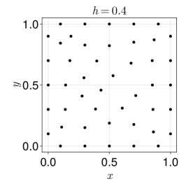
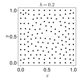
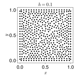
Figure 1: Irregular point clouds with different constant smoothing lengths $h$.

We calculate the relative discrete $L^{2}$ error of the numerical solution $u_{h}$ to the analytic reference solution $u$ by $\lVert u-u_{h}\rVert=\lVert u-u_{h}\rVert_{2}/\lVert u\rVert_{2}$ with the discrete $L^{2}$ norm

$$\lVert u\rVert_{2}=\left(\sum_{i=1}^{N}v_{i}u_{i}^{2}\right)^{\frac{1}{2}}.$$

For the integration weights $v_{i}$, we choose the Voronoi cell volumes $v_{i}=\lvert\Omega_{i}\rvert$ from equation 18 to obtain the property $\sum_{i=1}^{N}v_{i}=\lvert\Omega\rvert$.

We test the methods on Poisson’s equation (3) in section 4.1 and the heat equation (2) in section 4.2

4.1 Poisson’s equation

First, we study the behavior of the new operator using Poisson’s equation as in equation 3. We distinguish between problems with smooth diffusivity and discontinuous diffusivity.

Expanding the diffusion operator for a differentiable diffusivity $\lambda\in C^{1}(\Omega)$ and a sufficiently smooth analytic solution $u\in C^{2}(\Omega)$ as in equation 10 allows us to define the source term

$$q=-\Delta_{\lambda}u=-\langle\nabla\lambda,\nabla u\rangle-\lambda\Delta u.$$

For the elliptic interface test case, we assume that $\lambda$ is piecewise constant and has a jump on a $d-1$ dimensional manifold $\Gamma\subset\Omega$. For a smooth function $f\in C^{2}(\Omega)$ with $f|_{\Gamma}=0$, we define the analytic solution by

$$u=\frac{f}{\lambda}+c$$

with a constant $c$ to fulfill the homogeneous Dirichlet boundary condition. Because $f$ vanishes on the interface $\Gamma$, division by $\lambda$ introduces only a weak discontinuity. Hence, the resulting function is weakly differentiable, $u\in H^{1}(\Omega)$, with $\nabla u=\nabla f/\lambda$ and thus $\lambda\nabla u=\nabla f$. As a consequence, the source term

$$q=-\Delta_{\lambda}u=-\Delta f$$

is continuous.

Test case 1

(a) Analytic solution $u$.

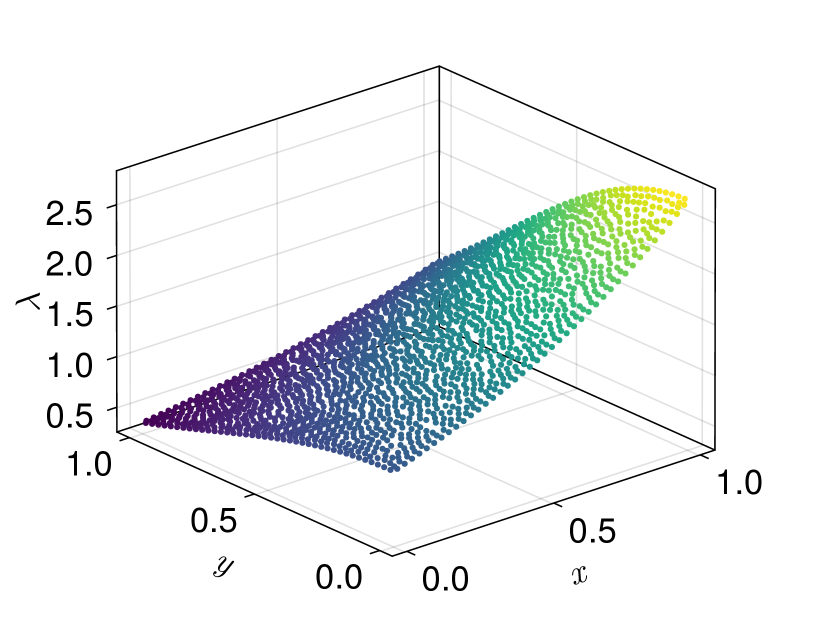
(b) Diffusivity $\lambda$.

Figure 2: Setup for test case 1.

Using the analytic solution $u(\bm{x})=\sin(\pi x_{1})\sin(\pi x_{2})$, we choose $\lambda(\bm{x})=\exp(x_{1}-x_{2}^{2})$, displayed in figure 2.

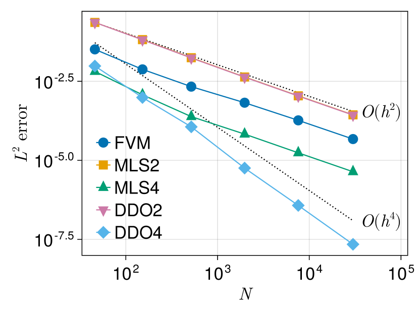
(a) Comparison of methods using arithmetic averaging for FVM and DDO$k$.

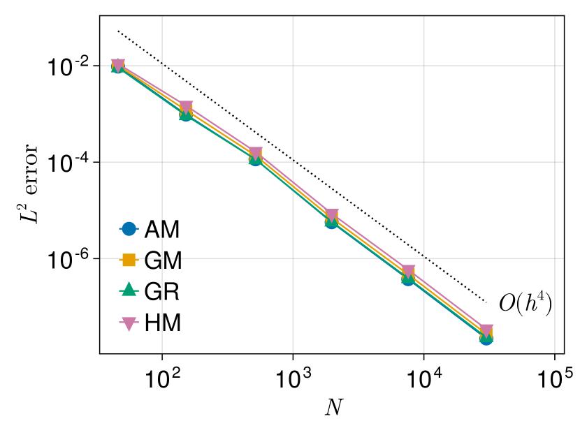
(b) Comparison of reconstruction methods using DDO4.

Figure 3: Relative $L^{2}$ error depending on the number of points $N$ for test case 1.

The results for the different methods are summarized in figure 3(a). For FVM and DDO$k$, we used arithmetic averaging to calculate the intermediate values $\lambda_{ij}$. We observe that FVM, MLS2, MLS4, and DDO2 are second-order accurate. While MLS2 and DDO2 achieve similar errors, FVM shows a lower error, with MLS4 producing an even lower error. Finally, DDO4 yields the lowest errors and fourth-order convergence, even though we only used first-order accurate arithmetic average reconstructions, in contrast to the second-order accurate gradient approximation for MLS4. The results suggest that the dominant error derived in Theorem 3.4 comes from the discrete Laplace operator and not from the reconstructions. In figure 3(b), we show that all reconstruction methods preserve the order of the underlying discrete Laplace operator and lead to almost the same errors in the example of DDO4.

Test case 2

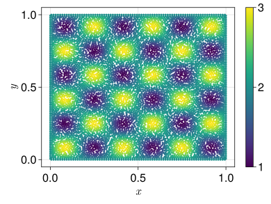
Figure 4: Diffusivity $\lambda$ for test case 2.

For this test case, we leave the analytic solution as in test case 1 and use a more challenging diffusivity $\lambda(\bm{x})=2+\sin(6\pi x_{1})\sin(6\pi x_{2})$, as shown in figure 4. Because of the local extrema, the averaging reconstructions might fail to reconstruct the function values at the mid-points $\bm{x}_{ij}$.

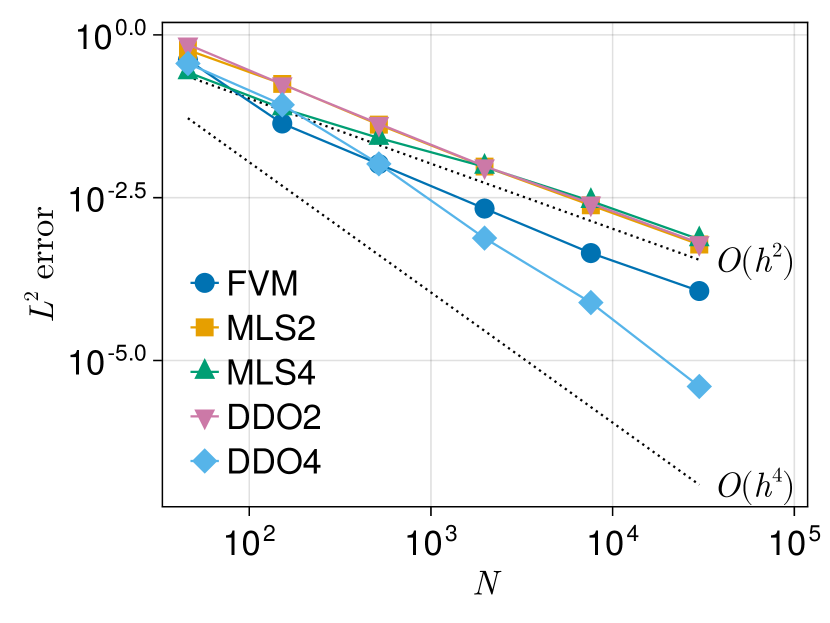
(a) Comparison of methods using arithmetic averaging for FVM and DDO$k$.

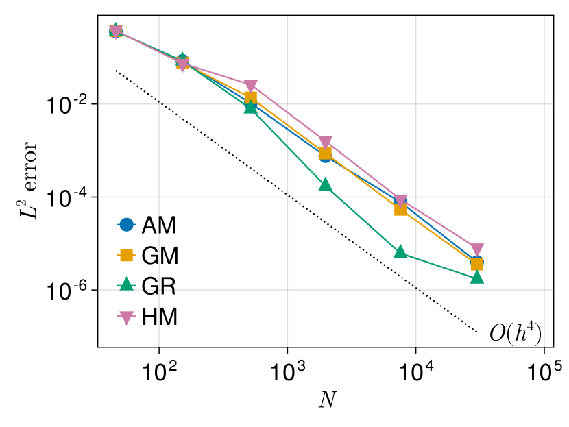
(b) Comparison of reconstruction methods using DDO4.

Figure 5: Relative $L^{2}$ error depending on the number of points $N$ for test case 2.

The results in figure 5(a) let us draw similar conclusions as in test case 1, with DDO4 being the only fourth-order method. Comparing the different reconstruction methods for DDO4 in figure 5(b), we observe that the gradient reconstruction slightly outperforms the averaging reconstructions. Nevertheless, all reconstructions conserve the fourth-order accuracy of the underlying discrete Laplace operator.

Test case 3

Now we consider a test case with a discontinuous diffusivity $\lambda$. With $c=\frac{3}{4}$, we choose $f(\bm{x})=\sin(\pi x_{1})\sin(\pi x_{2})-c$ and a piecewise constant diffusivity with a jump of eight orders of magnitude

$$\lambda(\bm{x})=\begin{cases}10^{8},&f(\bm{x})\geq 0,\\ 1,&f(\bm{x})<0.\end{cases}$$

The resulting interface $\Gamma=\set{\bm{x}\mid f(\bm{x})=0}$ can be seen in figure 6 along which $u$ has a weak discontinuity and $\lambda$ has a jump. The results in figure 7(a) show FVM and DDO$k$ with harmonic averaging.

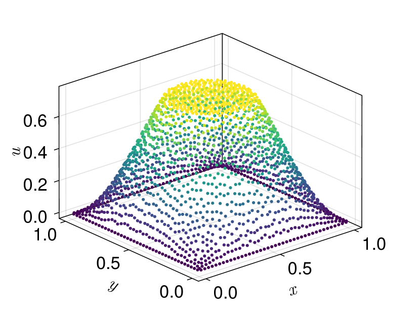
(a) Analytic solution $u$.

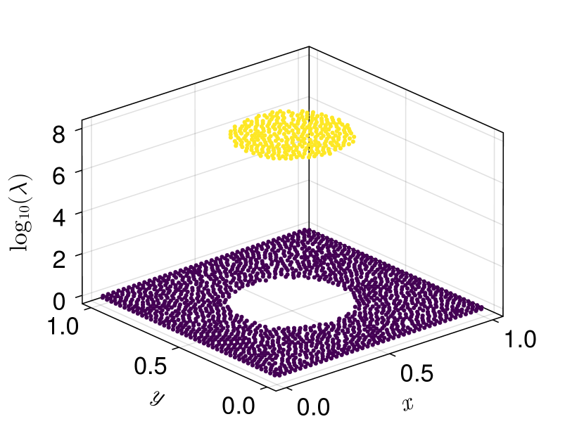
(b) Diffusivity $\lambda$.

Figure 6: Setup for test case 2.

MLS$k$ does not provide the correct solution, independent of the refinement $h$. The remaining methods are at least first-order accurate with FVM yielding the lowest errors and DDO2 the highest. FVM also shows second-order convergence for some refinement levels, especially for the first three and the last two refinement levels. This behavior is also present in the other methods but not so frequently. Nevertheless, this is a big advantage compared to the present MLS-based approach which fails to converge for this test case.

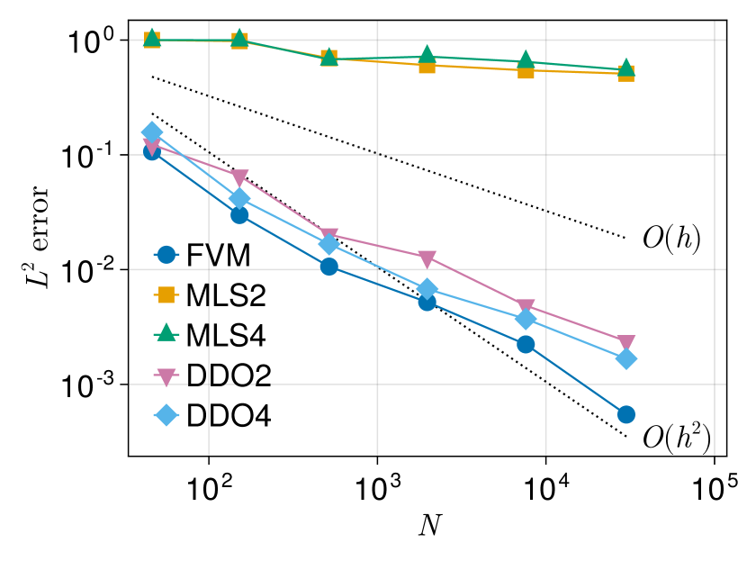
(a) Comparison of methods using harmonic averaging for FVM and DDO$k$.

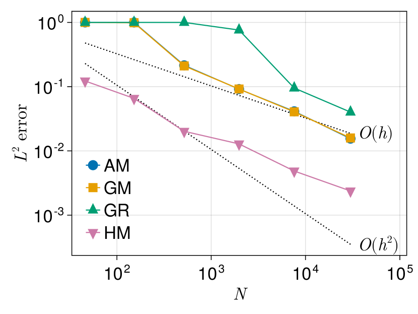
(b) Comparison of reconstruction methods using DDO2.

Figure 7: Relative $L^{2}$ error depending on the number of points $N$ for test case 3.

Comparing the reconstruction methods in figure 7(b), harmonic averaging clearly shows the lowest error with DDO2. We observed the same with FVM and DDO4. It may seem surprising that gradient reconstruction performs the worst. Because the gradients are based on the MLS approximation, the discrete gradient $\nabla_{i}\lambda$ becomes smeared-out, and especially for high discontinuities there is no guarantee that the reconstructions suffice to $\min(\lambda_{i},\lambda_{j})\leq\lambda_{ij}\leq\max(\lambda_{i},\lambda_{j}).$ Furthermore, non-positive reconstructions $\lambda_{ij}\leq 0$ cannot be excluded, leading to non-diagonally dominant operators and wrong results. This issue can be circumvented by other formulations of discrete gradients less susceptible to jumps, for example, a WENO technique [35]. This technique leads to a weak notion of the gradient and, in this example, to vanishing discrete gradients $\nabla_{i}\lambda\approx\bm{0}$. The gradient reconstruction scheme thus reduces to arithmetic averaging that performs worse than harmonic averaging.

4.2 Heat equation

To solve the heat equation (2), we multiply the analytic solutions from section 4.1, which we call $\bar{u}$, with a time-dependent function $a$ such that $u(\bm{x},t)=a(t)\bar{u}(\bm{x})$ is an analytic solution to the heat equation with the source term $q(\bm{x},t)=a^{\prime}(t)\bar{u}(\bm{x})-a(t)\Delta_{\lambda}\bar{u}(\bm{x}).$

Suchde [11] showed for a similar problem with a constant diffusivity $\lambda=1$ that the absence of diagonally dominant operators leads to severe instabilities in the numerical solution after a few time steps. Similarly to the test case used therein, we define $a(t)=\exp(-4t)$ for all test cases in this section and measure the relative $L^{2}$ error at $t=1$.

The time step size $\Delta t$ used in the implicit trapezoidal rule fulfills the CFL condition

$$\Delta t\leq 0.7\Delta x^{2},$$ (30)

where $\Delta x$ is the smallest distance between two points in the point cloud.

Test case 4

In this example, we use the analytic solution from test case 1 as $\bar{u}$. The results shown in figure 9 clearly show the expected convergence behavior, almost identical to the results in figure 3(a). FVM and DDO2 are second-order accurate, with FVM yielding lower errors, and DDO4 is fourth-order accurate. Because we applied first-order averaging to FVM and DDO, we show that the dominant error in time-dependent functions is due to the spatial discretization and not the temporal discretization or reconstruction function.

Test case 5

Similarly to test case 4, we use the analytic solution for the elliptic interface problem from test case 3 as $\bar{u}$. The results in figure 9 show that for this test case, we cannot reproduce the behavior as seen in figure 7(a). All methods converge with FVM yielding the lowest errors for the first three refinement levels. After that, the errors are almost constant. One reason could be that the time step sizes obtained from the CFL condition (30) are too large. Nevertheless, we observe first-order convergence on average for this selection of point clouds. Additionally, DDO2 and DDO4 are both on par with the mesh-based FVM.

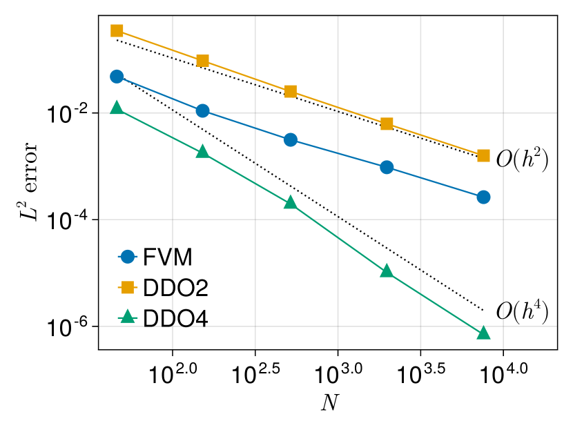
Figure 8: Relative $L^{2}$ error depending on the number of points $N$ for test case 4.

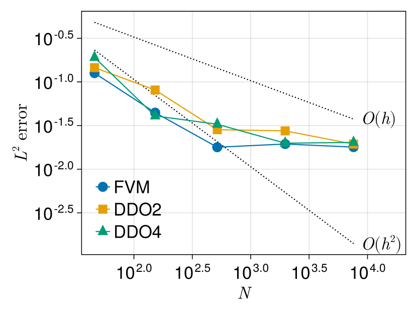
Figure 9: Relative $L^{2}$ error depending on the number of points $N$ for test case 5.

5 Final remarks

In this paper, we derived a new discretization method of the diffusion operator based on weighting the discrete Laplace operator by using reconstruction functions. We proved that the discrete diffusion operator preserves the consistency order from the discrete Laplace operator with additional error terms that arise from the reconstruction, and investigated diagonal dominance and enrichment properties. Other features such as conservation or the extension to anisotropic diffusion coefficients are relevant topics that might be featured in future research.

We tested the derived diffusion operator and showed that even first-order reconstructions conserve the fourth-order accuracy of the discrete Laplace operator for problems with smooth diffusivity. For interface problems, we demonstrated the applicability of the new discrete diffusion operator, and numerically showed first-order accuracy for such problems. The results were on par with the Voronoi-based finite volume method.

References

- [1] Jörg Kuhnert. General Smoothed Particle Hydrodynamics. Shaker Verlag, Aachen, Germany, 1999.
- [2] MESHFREE Homepage. https://www.meshfree.eu, 2023. Accessed 20-03-2023.
- [3] Isabel Michel, Tobias Seifarth, Jörg Kuhnert, and Pratik Suchde. A meshfree generalized finite difference method for solution mining processes. Computational Particle Mechanics, 8(3):561–574, 2021.
- [4] Lennart Veltmaat, Felix Mehrens, Hans-Josef Endres, Jörg Kuhnert, and Pratik Suchde. Mesh-free simulations of injection molding processes. Physics of Fluids, 34(3):033102, 2022.
- [5] C. R. Swaminathan and Vaughan R. Voller. On the enthalpy method. International Journal of Numerical Methods for Heat & Fluid Flow, 3(3):233–244, 1993.
- [6] Félix. R. Saucedo-Zendejo and Edgar. O. Reséndiz-Flores. Transient heat transfer and solidification modelling in direct-chill casting using a generalized finite differences method. Journal of Mining and Metallurgy, Section B: Metallurgy, 55(1):47–54, 2019.
- [7] Ivo Babuška. The finite element method for elliptic equations with discontinuous coefficients. Computing, 5(3):207–213, 1970.
- [8] Richard E. Ewing, Zhilin Li, Tao Lin, and Yanping Lin. The immersed finite volume element methods for the elliptic interface problems. Mathematics and Computers in Simulation, 50(1–4):63–76, 1999.
- [9] Chia-Ming Fan, Chi-Nan Chu, Božidar Šarler, and Tsung-Han Li. Numerical solutions of waves-current interactions by generalized finite difference method. Engineering Analysis with Boundary Elements, 100:150–163, 2019.
- [10] Po-Wei Li and Chia-Ming Fan. Generalized finite difference method for two-dimensional shallow water equations. Engineering Analysis with Boundary Elements, 80:58–71, 2017.
- [11] Pratik Suchde. Conservation and Accuracy in Meshfree Generalized Finite Difference Methods. PhD thesis, Technische Universität Kaiserslautern, 2018.
- [12] Benjamin Seibold. M-Matrices in Meshless Finite Difference Methods. PhD thesis, Technische Universität Kaiserslautern, 2006.
- [13] Michel Chipot. Elliptic Equations: An Introductory Course. Springer, 2009.
- [14] Heinrich Kraus, Jörg Kuhnert, Andreas Meister, and Pratik Suchde. A meshfree point collocation method for elliptic interface problems. Appl. Math. Model., 113:241–261, 2023.
- [15] Yanan Xing, Lina Song, Xiaoming He, and Changxin Qiu. A generalized finite difference method for solving elliptic interface problems. Mathematics and Computers in Simulation, 178:109–124, 2020.
- [16] Masood Ahmad, Siraj ul Islam, and Elisabeth Larsson. Local meshless methods for second order elliptic interface problems with sharp corners. Journal of Computational Physics, 416(109500):109500, 2020.
- [17] Oleg Davydov and Mansour Safarpoor. A meshless finite difference method for elliptic interface problems based on pivoted QR decomposition. Applied Numerical Mathematics, 161:489–509, 2021.
- [18] Qiushuo Qin, Lina Song, and Fan Liu. A meshless method based on the generalized finite difference method for three-dimensional elliptic interface problems. Computers & Mathematics with Applications, 131:26–34, 2023.
- [19] Young-Cheol Yoon and Jeong-Hoon Song. Extended particle difference method for weak and strong discontinuity problems: part I. Derivation of the extended particle derivative approximation for the representation of weak and strong discontinuities. Computational Mechanics, 53(6):1087–1103, 2014.
- [20] Do Wan Kim, Wing Kam Liu, Young-Cheol Yoon, Ted Belytschko, and Sang-Ho Lee. Meshfree point collocation method with intrinsic enrichment for interface problems. Computational Mechanics, 40(6):1037–1052, 2007.
- [21] Pratik Suchde and Jörg Kuhnert. A meshfree generalized finite difference method for surface PDEs. Computers & Mathematics with Applications, 78(8):2789–2805, 2019.
- [22] Elisabeth Larsson and Bengt Fornberg. A numerical study of some radial basis function based solution methods for elliptic PDEs. Computers & Mathematics with Applications, 46(5):891–902, 2003.
- [23] Natasha Flyer, Bengt Fornberg, Victor Bayona, and Gregory A. Barnett. On the role of polynomials in RBF-FD approximations: I. Interpolation and accuracy. Journal of Computational Physics, 321:21–38, 2016.
- [24] Victor Bayona, Miguel Moscoso, Manuel Carretero, and Manuel Kindelan. RBF-FD formulas and convergence properties. Journal of Computational Physics, 229(22):8281–8295, 2010.
- [25] Varun Shankar. The overlapped radial basis function-finite difference (RBF-FD) method: A generalization of RBF-FD. Journal of Computational Physics, 342:211–228, 2017.
- [26] Ilya D. Mishev. Finite volume methods on Voronoi meshes. Numerical Methods for Partial Differential Equations, 14(2):193–212, 1998.
- [27] Sławomir Milewski. Combination of the meshless finite difference approach with the monte carlo random walk technique for solution of elliptic problems. Computers & Mathematics with Applications, 76(4):854–876, 2018.
- [28] Thibault Jacquemin, Satyendra Tomar, Konstantinos Agathos, Shoya Mohseni-Mofidi, and Stéphane P. A. Bordas. Taylor-series expansion based numerical methods: A primer, performance benchmarking and new approaches for problems with non-smooth solutions. Archives of Computational Methods in Engineering, 27(5):1465–1513, 2020.
- [29] Zhiyin Zheng and Xiaolin Li. Theoretical analysis of the generalized finite difference method. Computers & Mathematics with Applications, 120:1–14, 2022.
- [30] Zhilin Li and Kazufumi Ito. Maximum principle preserving schemes for interface problems with discontinuous coefficients. SIAM Journal on Scientific Computing, 23(1):339–361, 2001.
- [31] Nathaniel Trask, Mauro Perego, and Pavel Bochev. A high-order staggered meshless method for elliptic problems. SIAM Journal on Scientific Computing, 39(2):A479–A502, 2017.
- [32] Tobias Seifarth. Numerische Algorithmen für gitterfreie Methoden zur Lösung von Transportproblemen. PhD thesis, Universität Kassel, 2018.
- [33] Edmond Kwan-Yu Chiu, Qiqi Wang, Rui Hu, and Antony Jameson. A conservative mesh-free scheme and generalized framework for conservation laws. SIAM Journal on Scientific Computing, 34(6):A2896–A2916, 2012.
- [34] Pratik Suchde, Thibault Jacquemin, and Oleg Davydov. Point cloud generation for meshfree methods: An overview. Archives of Computational Methods in Engineering, 30(2):889–915, 2023.
- [35] Oliver Friedrich. Weighted essentially non-oscillatory schemes for the interpolation of mean values on unstructured grids. Journal of Computational Physics, 144(1):194–212, 1998.