The role of individual compensation and acceptance decisions in crowdsourced delivery

Abstract

High demand, rising customer expectations, and government regulations are forcing companies to increase the efficiency and sustainability of urban (last-mile) distribution. Consequently, several new delivery concepts have been proposed that increase flexibility for customers and other stakeholders. One of these innovations is crowdsourced delivery, where deliveries are made by occasional drivers who wish to utilize their surplus resources (unused transport capacity) by making deliveries in exchange for some compensation. The potential benefits of crowdsourced delivery include reduced delivery costs and increased flexibility (by scaling delivery capacity up and down as needed). The use of occasional drivers poses new challenges because (unlike traditional couriers) neither their availability nor their behavior in accepting delivery offers is certain. The relationship between the compensation offered to occasional drivers and the probability that they will accept a task has been largely neglected in the scientific literature. Therefore, we consider a setting in which compensation-dependent acceptance probabilities are explicitly considered in the process of assigning delivery tasks to occasional drivers. We propose a mixed-integer nonlinear model that minimizes the expected delivery costs while identifying optimal assignments of tasks to a mix of professional and occasional drivers and their compensation. We propose an exact two-stage solution algorithm that allows to decompose compensation and assignment decisions for generic acceptance probability functions and show that the runtime of this algorithm is polynomial under mild conditions. Finally, we also study a more general case of the considered problem setting, show that it is NP-hard and propose an approximate linearization scheme of our mixed-integer nonlinear model. The results of our computational study show clear advantages of our new approach over existing ones.

Keywords: Crowdsourced delivery, occasional drivers, compensation schemes, acceptance uncertainty, crowdshipper behavior

1 Introduction

Fueled by the Covid-19 pandemic, e-tailing and same-day home delivery have continued to grow. This increase in demand and rising customer expectations are forcing providers to improve their efficiency in last-mile distribution. At the same time, technological advances and the proliferation of the sharing economy, such as Airbnb, car-sharing systems, and ride-hailing systems like Uber, have popularized the gig economy. In this new paradigm, instead of hiring employees on long-term contracts, employers (companies or individuals) can offer small, short-term tasks (usually through an online platform) and compensation for performing the task. Gig workers can then agree to perform that task in exchange for the advertised compensation. A prime example of the gig economy is crowdsourced delivery (Savelsbergh and Ulmer, 2022), which is one of the most prominent research directions in city logistics (Kaspi et al., 2022). Instead of using a traditional logistics system, a company can choose to offer delivery tasks to regular customers or other independent couriers (often referred to as occasional drivers) and compensate them accordingly. Crowdsourced delivery which has the potential to reduce overall delivery costs and increase the flexibility of delivery capacity, has already attracted interest from both industry and academia. Alnaggar et al. (2021) and Savelsbergh and Ulmer (2022) provide comprehensive overviews and classifications of industry applications and scientific contributions.

Crowdsourced delivery adds significant complexity to the planning process because the behavior and availability of occasional drivers is often not known in advance. Integrating the behavior of occasional drivers into planning decisions, especially with respect to task acceptance, is a major challenge in this domain (Savelsbergh and Ulmer, 2022). In the case of instant delivery (e.g., food orders), the inability to find an occasional driver for an offered task may lead to customer dissatisfaction or significant additional costs. In the classical models, occasional drivers are assumed to accept all tasks for which the compensation is high enough to compensate for the additional costs incurred by the drivers for the detour, see e.g. Archetti et al. (2016); Arslan et al. (2019). More recently, acceptance probabilities have been investigated through behavioral studies and surveys of occasional drivers, see e.g. Devari et al. (2017); Le and Ukkusuri (2019). Such acceptance probabilities were used as fixed parameters in the task allocation problem by Gdowska et al. (2018) and Santini et al. (2022). The effect of compensation schemes on acceptance behavior was investigated by Dayarian and Savelsbergh (2020), but only through a sensitivity analysis of fixed compensation options and acceptance thresholds drawn from a normal distribution. Barbosa et al. (2022) and Hou et al. (2022) integrate the impact of compensation on acceptance probabilities within task allocation. However, Barbosa et al. (2022) assume that the detour of all occasional drivers is the same for each task. Consequently, the compensations of all occasional drivers are identical. Hou et al. (2022) propose a sequential approach in which the compensation values are optimized for fixed task allocations that are decided in the first step.

Contribution and outline

This paper is the first to incorporate task-acceptance probabilities of occasional drivers, which depend on the operator’s compensation decisions, into an exact solution framework. To this end, we introduce a mixed-integer nonlinear programming (MINLP) formulation that optimizes the decision process by allowing for full flexibility in the compensations offered and the associated acceptance probabilities of occasional drivers. To model the latter, we introduce acceptance probability functions that estimate the probability that an occasional driver will accept a task. This estimation can be based on historical information, the attributes of occasional drivers and tasks, external factors, and the compensations offered. In our model, referred to as the Crowdshipping Assignment Problem with Compensation-Driven Acceptance Behavior (CAPCAB), we aim to minimize the total expected cost of assigning tasks by outsourcing them to either occasional (crowdsourced) drivers or to a third party logistics company, while ensuring that all delivery tasks are performed. Our model is applicable to several established crowdsourced delivery settings, see, e.g., Sampaio et al. (2019) for a classification. These include in-store deliveries in which occasional drivers (e.g., regular customers) are initially located at the pick-up location and multi-depot deliveries in which they first need to travel to a pick-up location as occurring, e.g., in meal delivery. Customer orders have to be delivered as quickly as possible via direct delivery, and multiple orders cannot be combined within a single trip by an occasional driver, as in Archetti et al. (2016); Ausseil et al. (2022).

Our main contributions can be summarized as follows:

• We introduce the CAPCAB, which considers (generic) compensation-dependent task acceptance probability functions of occasional drivers and allows to derive optimal compensations offered to them while minimizing the expected cost to the operator.

• We introduce a MINLP formulation for the CAPCAB (with generic acceptance probability functions) and show that it can be solved optimally via a two-stage approach that decomposes compensation and assignment decisions. We also show, that this two-stage approach which uses an exact linearization of our MINLP formulation allows to solve the CAPCAB in polynomial time for generic probability functions under mild conditions.

• We study two practically relevant classes of acceptance probability functions (linear and logistic acceptance probability functions) and derive explicit formulas for optimal compensation values in these cases.

• We study a generalization of the CAPCAB, show that it is NP-hard, and propose an approximate linearization scheme for an appropriately extended MINLP formulation.

• We conduct an extensive computational study and sensitivity analysis on the main model parameters. Our results show that the compensation scheme proposed in this work consistently and significantly outperforms alternative established compensation schemes from the literature. We also demonstrate that this scheme ensures higher satisfaction of occasional drivers by providing them with more and more successful offers. Finally, the extremely low runtimes on large instances consisting of 100 tasks and up to 150 occasional drivers and the computational complexity of the proposed method indicate that our approach can be applied to larger problem instances that could arise in real-life applications.

This paper is organized as follows. Section 2 summarizes the related literature. Section 3 formally introduces the problem studied in this paper, provides a MINLP formulation, and discusses the considered acceptance probability functions. Section 4 introduces the theoretical results that lead to the exact linearizations and polynomial-time solvability of CAPCAB. Section 5 focuses on the aforementioned generalization of the CAPCAB, shows that this variant is NP-hard, and introduces an approximate linearization scheme for this more general case. Section 6 details the setup of our computational study, whose results and findings are discussed in Section 7. We conclude in Section 8, where we also provide possible future research directions. The Appendix contains proofs of all theoretical results, and additional computational results .

2 Literature review

In this section, we review articles that address uncertainty in driver behavior and/or compensation optimization subjects in the context of crowdsourced delivery. The reviewed papers consist of those identified by Savelsbergh and Ulmer (2022), as well as more recent papers addressing both subjects. Table 1 provides an overview of these articles and classifies them according to three criteria: service type (following the classification of Sampaio et al. (2019)), compensation, and crowdshipper acceptance probability. An article is classified as driver dependent (or independent) if the attributes of occasional drivers are considered (or not considered) in the corresponding criterion. Integrated compensation indicates that compensation decisions are simultaneously made with other decisions. Finally, works considering compensation dependent acceptance probability model acceptance probability of occasional drivers as a function of compensation. In the following paragraph, we briefly summarize the articles that consider uncertainty in driver behavior without using acceptance probability functions. Section 2.1 discusses papers in which the compensation offered to drivers for performing tasks are treated as decisions that are independent of acceptance probabilities. Finally, Section 2.2 provides details on articles that assume a relationship between compensation decisions and acceptance probabilities.

Table 1: Literature overview

	Service Type		Compensation			Acceptance Probability
Paper	Multi-Depot	In-Store	Driver Independent	Driver Dependent	Integrated	Driver Independent	Driver Dependent	Compensation Dependent
Kafle et al. (2017)	✓
Gdowska et al. (2018)		✓				✓
Allahviranloo and Baghestani (2019)	✓
Mofidi and Pazour (2019)	✓
Dai and Liu (2020)	✓
Ausseil et al. (2022)	✓
Behrendt et al. (2022)	✓
Santini et al. (2022)		✓				✓
Dahle et al. (2019)	✓			✓	✓
Yildiz and Savelsbergh (2019)	✓		✓			✓
Cao et al. (2020)	✓			✓
Le et al. (2021)	✓			✓	✓
Barbosa et al. (2022)		✓	✓			✓		✓
Hou et al. (2022)		✓		✓			✓	✓
Our Work	✓	✓		✓	✓		✓	✓

Kafle et al. (2017) and Allahviranloo and Baghestani (2019) focus on a bid submission setting in which a planner obtains bids that contain information about tasks and compensation amounts required by occasional drivers. Mofidi and Pazour (2019) and Ausseil et al. (2022) consider approaches in which a planner offers menus of tasks to occasional drivers. Behrendt et al. (2022) study a scheduling problem that considers occasional drivers who are willing to commit to a time slot. Dai and Liu (2020) focus on a workforce allocation problem that considers the allocation of occasional drivers to different restaurants in a meal delivery setting. Finally, Gdowska et al. (2018) and Santini et al. (2022) study settings in which the acceptance probabilities of occasional drivers are considered but represented by fixed values.

2.1 Independent compensation decisions

Dahle et al. (2019) propose an extension of the pick-up and delivery vehicle routing problem with time windows in which the company owning the fleet can use occasional drivers to outsource some requests. They model the behavior of occasional drivers using personal threshold constraints, which indicate the minimum amount of compensation for which an occasional driver is willing to accept a task, and study the impact of the following three compensation schemes: fixed and equal compensation for each served request, compensation proportional to the cost of traveling from the pickup location to the delivery location, and compensation proportional to the cost of the detour taken by the occasional driver. Their results show that using occasional drivers can lead to savings of about 10-15%, even when using a sub-optimal compensation scheme. They also show that these savings can be further increased by using more complex compensation schemes.

Yildiz and Savelsbergh (2019) model a crowdsourced meal delivery system as a multi-server queue with general arrival and service time distributions to investigate which restaurants should be included in the network, what payments should be offered to couriers, and whether full-time drivers should be used. They study the trade-off between profit and service quality and analyze the impact of unit revenue and vehicle speed. They derive optimal compensation amounts analytically, considering per-delivery and per-mile schemes, with respect to the optimal service area. They also investigate the impact of a given acceptance probability on the service area and compensation.

Cao et al. (2020) consider a sequential packing problem to model task deliveries by occasional drivers and a professional fleet. In their setting, a distribution center receives delivery tasks at the beginning of a day, assigns bundles of tasks to occasional drivers during the day, and delivers the remaining tasks by the company-owned fleet at the end of the day. To model the arrival of occasional drivers, a marked Poisson process is proposed that specifies the time at which an occasional driver requests a task bundle and the bundle size. The arrival rate is assumed to be the same for each task bundle and is influenced by an incentive rate that allows an occasional driver to earn the same profit by delivering any bundle. They optimize the incentive rate that minimizes total delivery costs.

Le et al. (2021) integrate task assignment, pricing, and compensation decisions. They assume that an occasional driver will accept a task if the compensation is above a given threshold and below an upper bound that the operator is willing to offer. These (distance-dependent) thresholds are derived from real-world surveys. The authors evaluate flat and individual compensation schemes under different levels of supply and demand.

2.2 Compensation dependent acceptance probability

Barbosa et al. (2022) extend the problem proposed by Archetti et al. (2016) by integrating compensation decisions. As one of the few papers to date, they combine pricing, matching, and routing aspects while considering the possibility that occasional drivers may refuse tasks. The acceptance probability is modeled as a function of the compensation offered. However, the authors assume that the probability function is identical for each pair of occasional driver and task. This implies that decisions about compensations are reduced to defining a single compensation that is constant for each occasional driver offered a task. The considered problem is solved using a heuristic algorithm which builds upon the method proposed in Gdowska et al. (2018).

Hou et al. (2022) propose an optimization framework for a crowdsourced delivery service. They model the problem as a discrete event system, where an event is a task or a driver entering the system. A two-stage procedure is proposed to solve the problem. Tasks are assigned in the first stage, which focuses on minimizing the total detour of assigned tasks. In the second stage, optimal compensations are calculated that minimize the total delivery cost for the given task. The problem setting also considers the possibility that occasional drivers may refuse tasks, and the acceptance probabilities are determined by a binomial logit discrete choice model.

Studying the impact of compensation decisions on the acceptance behavior of occasional drivers has been identified as an important research direction. The first steps towards filling this research gap have been taken by Barbosa et al. (2022) and Hou et al. (2022). Barbosa et al. (2022) do not consider individual properties of driver-task pairs and solve the resulting problem heuristically. Even though Hou et al. (2022) consider compensations for each assigned pair individually, their sequential algorithm computes optimal compensations once the assignments are fixed. As a result, their approach lacks an evaluation of all possible task assignment-compensation combinations. We aim to overcome these shortcomings by making assignment and compensation decisions simultaneously while considering compensation-dependent acceptance behaviors of occasional drivers, and by proposing an exact method for solving the resulting optimization problem.

3 Problem definition

In the following, we formally introduce the Crowdshipping Assignment Problem with Compensation-Driven Acceptance Behavior. The CAPCAB aims to fulfill a set of online orders (tasks) $I$ by offering them to occasional drivers or outsourcing them to a third part logistics company (3PL). The set of occasional drivers $J$ represents ordinary customers and other independent couriers who express willingness to perform tasks from $I$. These drivers are not fully employed and perform individual delivery tasks on their own time. A solution to the CAPCAB allocates each task $i\in I$ either by offering the task to an occasional driver $j\in J$ or by outsourcing it to the 3PL who is assumed to perform the task at a costs $c_{i}\geq 0$. In the remainder, we refer to the 3PL as professional drivers to differentiate them from the occasional drivers.

Occasional drivers are offered a compensation for performing a task, and they can choose whether to accept the task given their own utility with regard to compensation. The compensation dependent acceptance probability $P_{ij}(C_{ij})$ specifies the probability that an occasional driver $j\in J$ will accept an offer to perform a task $i\in I$ when offered a compensation of $C_{ij}\geq 0$. Tasks refused by an occasional driver must be performed by a professional driver, incurring a penalized cost $c_{i}^{\prime}\geq c_{i}$ to the company.

A feasible solution of the CAPCAB can be described as a one-to-one assignment $A\subset I_{\mathrm{o}}\times J_{\mathrm{o}}$ where $I_{\mathrm{o}}\subseteq I$ is the set of tasks offered to a subset of the occasional drivers $J_{\mathrm{o}}\subseteq J$. Every other task $i\in I\setminus I_{\mathrm{o}}$ is performed by a professional driver, while no tasks are offered to the occasional drivers belonging to $J\setminus J_{\mathrm{o}}$. The total expected cost of such a solution is represented by

$$\sum_{i\in I\setminus I_{\mathrm{o}}}c_{i}+\sum_{(i,j)\in A}\left(P_{ij}(C_{ij})C_{ij}+(1-P_{ij}(C_{ij}))c_{i}^{\prime}\right),$$ (1)

which sums up the total delivery cost to perform each task $i\in I\setminus I_{\mathrm{o}}$ by professional drivers and the expected cost stemming from offering compensation $C_{ij}$ to driver $j$ to perform task $i$, for each $(i,j)\in A$. The expected cost for each $(i,j)\in A$ is given by the compensation $C_{ij}$ times the probability $P_{ij}(C_{ij})$ that occasional driver $j$ will accept task $i$, plus the penalized cost $c^{\prime}_{i}$ to perform task $i$, times the probability $1-P_{ij}(C_{ij})$ that occasional driver $j$ will refuse the task. The objective of the CAPCAB is to define the sets $I_{\mathrm{o}}$ and $J_{\mathrm{o}}$, their one-to-one assignment $A\subset I_{\mathrm{o}}\times J_{\mathrm{o}}$, and the compensation $C_{ij}$ for each $(i,j)\in A$ in such a way that the expected total cost is minimized.

(a) Instance and solution.

(b) OD 1 accepts task 2.

(c) OD 1 refuses task 2.

Figure 1: An instance and a solution of the CAPCAB in which occasional driver (OD) 1 is offered a compensation of $C_{21}$ for task 2. Figures 1(b) and 1(c) visualize the deliveries when OD 1 accepts or refuses task 2, respectively.

Figure 1 provides an instance of the CAPCAB and illustrates the allocation of tasks to occasional and professional drivers, as well as the role of the acceptance probability. Within this example, we consider a scenario with two tasks and two occasional drivers, i.e., $I=\{1,2\}$ and $J=\{1,2\}$. The figure indicate the store (in the middle of the figure) and the delivery location of the two tasks as well as the home location of the occasional drivers (to illustrate the potential detour of potential occasional drivers to complete the task). For simplicity, we assume that both occasional drivers are initially located at the central store. Figure 1(a) illustrates a solution for the instance in which task 1 is assigned to a professional driver (at cost $c_{1}$) and compensation $C_{21}$ is offered to occasional driver 1 for performing task 2, i.e., $I_{\mathrm{o}}=\{2\}$, $J_{\mathrm{o}}=\{1\}$, and $A=\{(2,1)\}$. Occasional driver 2 drives directly from the central depot to its final destination while occasional driver 1 must accept or refuse the task. With probability $P(C_{21})$, occasional driver 1 will accept the task (leading to total costs of $C_{21}$ + $c_{1}$) in which case they perform the task and then drive to their final destination, see Figure 1(b). With probability $1-P(C_{21})$, they refuse the task and drive directly to their final destination. In this case, an additional professional driver must be used to perform task 1, and the total costs are equal to $c_{1}+c_{2}^{\prime}$, see Figure 1(c). Therefore, the expected total cost of the solution equals $P(C_{21})(C_{21}+c_{1})+(1-P(C_{21}))(c_{1}+c^{\prime}_{2})$.

Assumptions

The above definition of the CAPCAB assumes a static scenario with complete information, where the set of tasks $I$ and the set of available occasional drivers $J$ are known at the time of the assignment (e.g., by requiring the occasional drivers to sign up for a certain time slot in order to be offered tasks). While the availability of an occasional driver is certain, their acceptance behavior is probabilistic. Within our framework, we only assume that the underlying compensation-dependent acceptance probability functions $P_{ij}:\mathbb{R}_{+}\mapsto[0,1]$ are separable for each $i\in I$ and $j\in J$, i.e., that the probability of driver $j\in J$ for task $i\in I$ does not depend on other tasks $i^{\prime}\in I\setminus\{i\}$ or compensations offered to other drivers $j^{\prime}\in J\setminus\{j\}$, nor on their acceptance decisions. We argue that the latter assumption is realistic in the considered static setting where occasional drivers receive individual offers and thus have little opportunity to exchange information. Notice that information exchange between occasional drivers after their acceptance or refusal, which may influence their behavior, can be incorporated into the acceptance probabilities before each time slot in a dynamic setting while obeying the separability assumption. Finally, we also assume that $P_{ij}(0)=0$ for all $i\in I,j\in J$, i.e., no occasional driver works for free and, consequently, is never offered a task without compensation. In practice, we assume that historical information on driver decisions combined with characteristics of tasks and occasional drivers (e.g., their destinations or historical acceptance behavior), and external factors allow to estimate the probability function.

3.1 Mixed integer nonlinear programming formulation

Next, we introduce an MINLP formulation (2) for the CAPCAB that uses three sets of decision variables. Variables $y_{i}\in\{0,1\}$ indicate whether task $i\in I$ is performed by a professional driver, and variables $x_{ij}\in\{0,1\}$ indicate whether task $i\in I$ is offered to occasional driver $j\in J$. Variables $C_{ij}\geq 0$ represent the compensation offered to occasional driver $j\in J$ for performing task $i\in I$.

$$\min\quad \sum_{i\in I}\left(c_{i}y_{i}+\sum_{j\in J}\left(P_{ij}(C_{ij})C_{ij}+(1-P_{ij}(C_{ij}))c^{\prime}_{i}\right)x_{ij}\right)$$ (2a)

s.t. $$\sum_{i\in I}x_{ij}\leq 1 j\in J$$ (2b)

$$\sum_{j\in J}x_{ij}+y_{i}=1 i\in I$$ (2c)

$$C_{ij}\leq U_{ij}x_{ij} i\in I,\ j\in J$$ (2d)

$$x_{ij}\in\{0,1\} i\in I,\ j\in J$$ (2e)

$$y_{i}\in\{0,1\} i\in I$$ (2f)

$$C_{ij}\geq 0 i\in I,\ j\in J$$ (2g)

The objective function (2a) minimizes the expected total cost. Constraints (2b) ensure that at most one task is offered to each occasional driver. Equations (2c) ensure that each task is either offered to an occasional driver or performed by a professional driver. Inequalities (2d) ensure that the compensation offered is not greater than a given upper bound $U_{ij}$ if task $j\in J$ is offered to occasional driver $i\in I$. Note that the cost $c_{i}$ of a professional driver for task $i\in I$ can always be used as such an upper bound, since it will never be optimal to offer compensation that exceeds this value. Furthermore, constraints (2d) also force $C_{ij}$ to zero if task $i\in I$ is not offered to occasional driver $j\in J$. Finally, constraints (2e)–(2g) define the domains of the variables. The difficulty of formulation (2) depends significantly on the considered probability function $P_{ij}:\mathbb{R}_{+}\mapsto[0,1]$ of occasional drivers $j\in J$ for tasks $i\in I$. In Section 4, we discuss a two-stage solution framework considering a general acceptance probability function. In the remainder of this section, we introduce two probability functions that can be used to model realistic acceptance behavior and discuss their use within the solution framework in Section 4.

3.2 Linear acceptance probability

One way to model the acceptance behavior of occasional drivers is to assume that their willingness to perform a task increases linearly with the compensation offered. Campbell and Savelsbergh (2006) propose a linear approach to model the time slot selection behavior of customers in the context of attended home delivery services. We adopt their idea to model the acceptance behavior of occasional drivers. For each task-driver pair, we assume an initial acceptance probability that depends on the pair’s characteristics. We also assume that this probability can be increased linearly by the amount of compensation offered, at a rate that also depends on the pair’s characteristics. Besides task specific characteristics such as distance or weight, these can also include other factors such as weather and traffic levels. Such linear acceptance models allow avoiding the oversimplified assumption of a given (task-specific) threshold above which an occasional driver will always perform a task. A linear model also has the advantage of having a small number of parameters that need to be estimated. We consider a linear model in which we assume that occasional driver $j\in J$ accepts task $i\in I$ with a given base probability $\alpha_{ij}$, $0\leq\alpha_{ij}\leq 1$, if the compensation offered is greater than zero. Parameter $\beta_{ij}>0$ specifies the rate at which the acceptance probability of occasional driver $j\in J$ increases for task $i\in I$ for a given compensation $C_{ij}$. Hence, the probability function is formally defined as

$$P_{ij}(C_{ij})=\begin{cases}0&\mbox{if $C_{ij}=0$}\\ \min\{\alpha_{ij}+\beta_{ij}C_{ij},1\}&\mbox{ otherwise }\end{cases},\quad i\in I,\ j\in J.$$ (3)

Considering function (3) in formulation (2), we first observe that there always exists an optimal solution in which $C_{ij}>0$ if task $i\in I$ is offered to occasional driver $j\in J$, i.e., if $x_{ij}=1$. Since the acceptance probability for a compensation of zero is equal to zero, the alternative solution in which task $j$ is performed by a professional driver is always at least as good (recall that we assumed that $c_{i}^{\prime}\geq c_{i}$). Similarly, it is never optimal to offer a compensation that exceeds the cost of a professional driver for the same task, or that exceeds the minimum compensation that leads to an acceptance probability equal to one. Thus, $\min\{c_{i},\frac{1-\alpha_{ij}}{\beta_{ij}}\}$ is an upper bound on the compensation offered to occasional driver $j\in J$ for task $i\in I$ that can be used to (possibly) strengthen the upper bounds $U_{ij}$ in constraints (2d). Consequently, the variant of formulation (2) for the linear acceptance probability case is obtained by replacing the objective function (2a) by

$$\min\quad \sum_{i\in I}\left(c_{i}y_{i}+\sum_{j\in J}[(\alpha_{ij}+\beta_{ij}C_{ij})C_{ij}+(1-\alpha_{ij}-\beta_{ij}C_{ij})c^{\prime}_{i}]x_{ij}\right).$$ (4)

3.3 Logistic acceptance probability

An alternative to modeling the acceptance behavior of occasional drivers that has been suggested in the literature is the use of logistic regression models. Devari et al. (2017) propose a logistic regression model to model the acceptance behavior of occasional drivers for performing a delivery for their friends. Similarly, Le and Ukkusuri (2019) propose a binary-logit model where the willingness to work as an occasional driver is considered a dependent variable. Logistic regression is particularly appealing when historical or experimental data are available on task and driver attributes, external factors, the compensation offered for tasks and the resulting acceptance decisions. Such data can be used to fit a logistic regression model that predicts the acceptance probabilities of occasional drivers. Using parameters $\gamma_{ij}$, which subsumes the impact of all predictors other than the compensation, and $\delta_{ij}>0$, logistic acceptance probabilities are modeled using functions

$$P_{ij}(C_{ij})=\begin{cases}0&\mbox{if $C_{ij}=0$}\\ \frac{1}{1+e^{-(\gamma_{ij}+\delta_{ij}C_{ij})}}&\mbox{ otherwise}\end{cases},\quad i\in I,\ i\in J.$$ (5)

A nonlinear model for the CAPCAB when considering logistic acceptance probabilities is obtained from (2) if the objective function (2a) is replaced by

$$\min\quad \sum_{i\in I}\left(c_{i}y_{i}+\sum_{j\in J}[(\frac{1}{1+e^{-(\gamma_{ij}+\delta_{ij}C_{ij})}})C_{ij}+(1-\frac{1}{1+e^{-(\gamma_{ij}+\delta_{ij}C_{ij})}})c^{\prime}_{i}]x_{ij}\right).$$ (6)

4 Mixed integer linear programming reformulations

A major advantage of the CAPCAB over previously introduced models is its integration of assignment and compensation decisions, as well as its consideration of the uncertain acceptance behavior of occasional drivers. However, these aspects pose a significant challenge to the design of well-performing solution methods that derive optimal assignment and compensation decisions. In this section, we show how to overcome this challenge by exploiting some of the assumptions made in the CAPCAB. We will show that, under certain conditions, the CAPCAB can be solved optimally using a two-phase approach that first identifies optimal compensation values that are used as input to the second phase, in which assignment decisions are made. We also provide explicit formulas for optimal compensation values in the case of linear and logistic acceptance probabilities. These results allow us to reformulate MINLP (2) and its variants for the latter two acceptance probability functions as mixed-integer linear programs (MILPs). They also imply that the CAPCAB can be solved in polynomial time whenever the first-phase problem of identifying optimal compensation values can be solved in polynomial time.

The main property required for the results introduced below is that the compensation and acceptance decisions are separable. This property holds for the CAPCAB since the acceptance probability functions are assumed to be independent of each other (for each pair of task and occasional driver) and since the considered setting does not include constraints that limit the operator’s choice, such as cardinality or budget limits on the tasks offered to occasional drivers. Theorem 1 reveals that the separability of compensation and acceptance decisions allows for the identification of optimal compensation values independent of the task allocation decisions. The latter is made more explicit in Corollary 1.

Theorem 1.

Consider an arbitrary instance of the CAPCAB. There exists an optimal solution for this instance in which the (optimal) compensation values $C_{ij}^{*}$ are equal to

$$C^{*}_{ij}=\mathrm{argmin}_{C_{ij}\geq 0}~{}P_{ij}(C_{ij})(C_{ij}-c^{\prime}_{i})$$

if task $i\in I$ is offered to occasional driver $j\in J$. Furthermore, compensations $C_{ij}^{*}$ for tasks $i\in I$ that are not offered to occasional driver $j\in J$ can be set to an arbitrary (non-negative) value.

Proof.

Provided in Appendix A. ∎

Corollary 1.

There exists an optimal solution for an arbitrary instance of the CAPCAB that can be identified by solving formulation (2) while setting compensation values equal to

$$C_{ij}^{*}=\mathrm{argmin}_{C_{ij}\geq 0}P_{ij}(C_{ij})(C_{ij}-c^{\prime}_{i})$$ (7)

for each task $i\in I$ and every occasional driver $j\in J$.

A major consequence of Corollary 1 is that optimal compensation values, which can be calculated according to Equation (7), are independent of the other decisions, i.e., which tasks to assign to professional drivers and which tasks to offer to which occasional driver. Therefore, we can first calculate the compensation values and then identify optimal assignment decisions using the MILP formulation (9) in which cost parameters ${\bar{c}}^{*}_{ij}$ are set to

$${\bar{c}}^{*}_{ij}=P_{ij}(C_{ij}^{*})C_{ij}^{*}+(1-P_{ij}(C^{*}_{ij}))c^{\prime}_{i}$$ (8)

for each $i\in I$ and $j\in J$. As in formulation (2), variables $y_{i}\in\{0,1\}$ indicate whether task $i\in I$ is performed by a professional driver and variables $x_{ij}\in\{0,1\}$ indicate whether it is offered to occasional driver $j\in J$.

$$\min\quad \sum_{i\in I}c_{i}y_{i}+\sum_{i\in I}\sum_{j\in J}{\bar{c}}^{*}_{ij}x_{ij}$$ (9a)

s.t. $$\sum_{i\in I}x_{ij}\leq 1 j\in J$$ (9b)

$$\sum_{j\in J}x_{ij}+y_{i}=1 i\in I$$ (9c)

$$x_{ij}\in\{0,1\} i\in I,\ j\in J$$ (9d)

$$y_{i}\in\{0,1\} i\in I$$ (9e)

Constraints (9b) and (9c) ensure that each occasional driver is offered at most one task, and that each task is either offered to an occasional driver or assigned to a professional driver. Overall, it is easy to see that formulation (9) is equivalent to a standard assignment problem (with special “assignment” variables $y_{i}$ for each $i\in I$). Consequently, Corollary 2 follows, since formulation (9) can be solved in polynomial time due to its totally unimodular constraint matrix.

Corollary 2.

The CAPCAB can be solved in polynomial time if the compensation and acceptance decisions are separable and optimal compensation values $C^{*}_{ij}$ for tasks $i\in I$ and occasional drivers $j\in J$ can be identified in polynomial time.

Propositions 1 and 2 provide explicit formulas for optimal compensations in instances of the CAPCAB if the acceptance behavior of occasional drivers is modeled using linear or logistic acceptance probability functions, respectively, as introduced in Section 3. Thus, such instances satisfy the conditions of Corollary 2 and can be solved in polynomial time.

Proposition 1.

Consider an instance of the CAPCAB in which the acceptance behavior of occasional drivers is modeled using the linear acceptance probability function

$$P_{ij}(C_{ij})=\begin{cases}0&\mbox{if $C_{ij}=0$}\\ \min\{\alpha_{ij}+\beta_{ij}C_{ij},1\}&\mbox{ otherwise }\end{cases},\quad i\in I,\ j\in J.$$ (10)

There exists an optimal solution for this instance with compensation values $C_{ij}^{*}=\frac{c^{\prime}_{i}}{2}-\frac{\alpha_{ij}}{2\beta_{ij}}$ for each task $i\in I$ and occasional driver $j\in J$.

Proof.

Provided in Appendix A. ∎

Proposition 2.

Consider an instance of the CAPCAB in which the acceptance behavior of occasional drivers is modeled using the logistic acceptance probability function

$$P_{ij}(C_{ij})=\begin{cases}0&\mbox{if $C_{ij}=0$}\\ \frac{1}{1+e^{-(\gamma_{ij}+\delta_{ij}C_{ij})}}&\mbox{ otherwise}\end{cases},\quad i\in I,\ i\in J.$$ (11)

There exists an optimal solution to that instance with compensation values $C_{ij}^{*}=-\frac{W(e^{\gamma_{ij}+\delta_{ij}c^{\prime}_{i}-1})-\delta_{ij}c^{\prime}_{i}+1}{\delta_{ij}}$ for each task $i\in I$ and occasional driver $j\in J$, in which $W(\cdot)$ is the Lambert $W$ function.

Proof.

Provided in Appendix A. ∎

5 The CAPCAB without separability

In this section, we discuss a generalization of the CAPCAB in which the decisions about which tasks to offer to occasional drivers and the corresponding compensation are not independent of each other. This occurs, for example, when the operator has to respect (strategic) considerations that limit the number of tasks offered to occasional drivers or the budget available for such offers. In this section, we assume that the relevant limitations can be modeled as a set of $L$ linear constraints involving assignment and compensation decisions. Using notation $a_{ij}^{\ell}$ and $b_{ij}^{\ell}$ for each $i\in I$, $j\in J$, and $\ell\in\{1,\dots,L\}$ to denote the coefficients associated to these two sets of variables and $B^{\ell}$ for the corresponding (resource) limits, the considered set of constraints is written as

$$\sum_{i\in I}\sum_{j\in J}(a_{ij}^{\ell}x_{ij}+b_{ij}^{\ell}C_{ij})\leq B^{\ell}, \ell\in\{1,\dots,L\}.$$ (12)

A cardinality constraint on the total number of tasks offered to occasional drivers can, e.g., be realized by setting $a_{ij}^{\ell}=1$ and $b_{ij}^{\ell}=0$ for all $i\in I$ and $j\in J$ while $a_{ij}^{\ell}=0$ and $b_{ij}^{\ell}=1$ holds for a constraint limiting the overall budget offered to occasional drivers.

Proposition 3 shows that the inclusion of non-separability constraints (12) implies NP-hardness of the resulting variant of the CAPCAB, which we call the Crowdshipping Assignment Problem with Compensation-Driven Acceptance Behavior without Separability (CAPCABwS).

Proposition 3.

The CAPCABwS is strongly NP-hard.

Proof.

Provided in Appendix A. ∎

While considering the above set of constraints related to operator choices, we still assume that the acceptance decisions of occasional drivers depend only on the task and compensation offered, i.e., the acceptance probability functions $P_{ij}(C_{ij})$ are still applicable. Thus, while the results concerning optimal compensation decisions from Section 4 and the two-phase solution approach are no longer applicable, the objective function (2a) can be decomposed for each $i\in I$ and $j\in J$, which is exploited in Proposition 4.

Proposition 4.

The nonlinear objective function (2a) in formulation (2) can be replaced by

$$\sum_{i\in I}c_{i}y_{i}+\sum_{i\in I}\sum_{j\in J}(f_{ij}(C_{ij})+g_{ij}(x_{ij})).$$ (13)

Thereby, $f_{ij}(C_{ij})$ is a nonlinear function depending on $C_{ij}$, and $g_{ij}(x_{ij})$ is a linear function in $x_{ij}$. In the case of generic acceptance probability functions $P_{ij}(C_{ij})$, we have $f_{ij}(C_{ij})=P_{ij}(C_{ij})(C_{ij}-c_{i}^{\prime})$ and $g_{ij}(x_{ij})=c_{i}^{\prime}x_{ij}$.

Proof.

Provided in Appendix A. ∎

Proposition 4 implies that a piecewise linear approximation of the nonlinear objective function (2a) can be derived using standard techniques. Thus, for each $i\in I$ and $j\in J$, we use a discrete set of possible compensation values $\{u_{ij}^{k}:k\in\{1,\dots,K\}\}$ such that $u_{ij}^{1}=0$, $u_{ij}^{K}=U_{ij}$, $u_{ij}^{k-1}<u_{ij}^{k}$, $k\in\{2,\dots,K\}$, together with non-negative variables $w_{ij}^{k}\geq 0$, $k\in\{1,\dots,K\}$. Since the nonlinear functions $f_{ij}(C_{ij})$ are not necessarily convex, formulation (14) also uses binary variables $v_{ij}^{k}\in\{0,1\}$ for each $i\in I$, $j\in J$, and $k\in\{1,\dots,K-1\}$. Here, $v_{ij}^{k}=1$ indicates that $u_{ij}^{k}\leq C_{ij}\leq u_{ij}^{k+1}$.

$$\min\quad \sum_{i\in I}c_{i}y_{i}+\sum_{i\in I}\sum_{j\in J}\left(\sum_{k=1}^{K}f_{ij}(u_{ij}^{k})w_{ij}^{k}+g_{ij}(x_{ij})\right)$$ (14a)

s.t. $$\eqref{eq:minlp:oc:assignment}-\eqref{eq:minlp:y},\eqref{eq:non-separable}$$

$$\sum_{k=1}^{K}u_{ij}^{k}w_{ij}^{k}\leq U_{ij}x_{ij} i\in I,\ j\in J$$ (14b)

$$w_{ij}^{1}\leq v_{ij}^{1} i\in I,\ j\in J$$ (14c)

$$w_{ij}^{k}\leq v_{ij}^{k-1}+v_{ij}^{k} i\in I,j\in J,\ k\in\{2,\dots,K-1\}$$ (14d)

$$w_{ij}^{K}\leq v_{ij}^{K-1} i\in I,\ j\in J$$ (14e)

$$\sum_{k=1}^{K-1}v_{ij}^{k}=1 i\in I,\ j\in J$$ (14f)

$$\sum_{k=1}^{K}w_{ij}^{k}=1 i\in I,\ j\in J$$ (14g)

$$v_{ij}^{k}\in\{0,1\} i\in I,\ j\in J,\ k\in\{1,\dots,K-1\}$$ (14h)

$$w_{ij}^{k}\geq 0 i\in I,\ j\in J,\ k\in\{1,\dots,K\}\$$ (14i)

The objective function (14a) is a piecewise linear approximation of the one introduced in Proposition 4 using the discrete set of compensation values $u_{ij}^{k}$ and variables $w_{ij}^{k}$. Recall that $g_{ij}(x_{ij})$ is a linear function. As described in Section 3.1, constraints (2b)-(2f) ensure that at most one task is offered to an occasional driver and that each task is either performed by a professional driver, or offered to an occasional driver. They also define the domains of variables $x_{ij}$ and $y_{i}$ for tasks $i\in I$ and occasional drivers $j\in J$. Constraints (12) have been introduced at the beginning of this section while inequalities (14b) are constraints $C_{ij}\leq U_{ij}x_{ij}$ rewritten using the identity $\sum_{k=1}^{K}u_{ij}^{k}w_{ij}^{k}=C_{ij}$. Finally, (14c)–(14i) are standard constraints used to model piecewise linear approximations, see, e.g., Nemhauser and Wolsey (1988) for further details.

Propositions 5 and 6 detail how formulation (14) can be modified when the acceptance behavior is modeled using a linear and logistic acceptance probability function, respectively.

Proposition 5.

Consider an arbitrary instance of the CAPCABwS in which the acceptance behavior of occasional drivers is modeled using the linear probability function (3). Then, Proposition 4 applies for $f_{ij}(C_{ij})=\beta_{ij}C_{ij}^{2}+(\alpha_{ij}-\beta_{ij}c_{i}^{\prime})C_{ij}$ and $g_{ij}(x_{ij})=c_{i}^{\prime}(1-\alpha_{ij})x_{ij}$.

Furthermore, variables $v_{ij}^{k}$, $i\in I$, $j\in J$, $k\in\{1,\dots,K-1\}$ and constraints (14c)–(14f) involving them are redundant in formulation (14) and can therefore be removed.

Proof.

Provided in Appendix A. ∎

Proposition 6.

Consider an arbitrary instance of the CAPCABwS in which the acceptance behavior of occasional drivers is modeled using the logistic probability function (5). Then, Proposition 4 applies for $g_{ij}(x_{ij})=c_{i}^{\prime}x_{ij}$ and $f_{ij}(C_{ij})=\begin{cases}0&\mbox{ if $C_{ij}=0$}\\ \frac{C_{ij}-c_{i}^{\prime}}{1+e^{-\gamma_{ij}-\delta_{ij}C_{ij}}}&\mbox{ otherwise}\end{cases}$.

Proof.

Provided in Appendix A. ∎

6 Experimental setup

In this section, we describe our benchmark instances, provide further details on the parameters of the considered acceptance probability functions, and introduce alternative compensation models inspired by the literature that we use to evaluate our approach.

6.1 Instances

As a relatively new area of research, the field of crowdsourced delivery still lacks established benchmark libraries. Most existing studies use instances from the VRP literature (e.g., Archetti et al. (2016); Barbosa et al. (2022)) or randomly generated synthetic instances (e.g., Arslan et al. (2019); Dayarian and Savelsbergh (2020)). Since the instances used in these works do not consider acceptance probabilities, we generate a new set of synthetic instances. To this end, we simulate an in-store delivery setting, where occasional drivers are assumed to be regular in-store customers who are willing to deliver a task en route. We generate destinations for occasional drivers and tasks uniformly at random in a $200\times 200$ plane. The coordinates of these locations are rounded to two decimal places. The store is assumed to be located in the center of the plane and coincides with the initial locations of all occasional drivers. We assume that the professional delivery cost $c_{i}$ for each task $i\in I$ is equal to the Euclidean distance between the task delivery point and the depot. Note that, since each task is identified with its origin and destination, the costs for professional and occasional drivers can be incorporated in the respective parameters without explicitly including these locations in the model. Therefore, our model generalizes problems consisting of tasks with different origins and destinations such as meal delivery, as well as tasks with single origin and different destinations such as in-store customer settings. Each instance is characterized by a combination of the following three parameters:

1. The number of occasional drivers $|J|\in\{50,75,\dots,150\}$.

2. A penalty parameter $\rho\in\{0,0.05,\dots,0.25\}$ that defines the relative increase in professional delivery costs if an occasional driver rejects an offer, i.e., $c_{i}^{\prime}=(1+\rho)c_{i}$, $\forall i\in I$.

3. A parameter $\mu\in\{0,0.1,\dots,1\}$ that affects the acceptance probabilities of occasional drivers and, in particular, their sensitivity towards making detours when performing deliveries. In the linear case, this parameter is used to define the base probability $\alpha_{ij}$ for each $i\in I$ and $j\in J$ via a weighted distance utility $\nicefrac{{\mu d_{j}}}{{(d_{i}+d_{ij})}}$, i.e., $\alpha_{ij}=\nicefrac{{\mu d_{j}}}{{(d_{i}+d_{ij})}}$. Here, $d_{k}$ is the Euclidean distance between the store and the destination of $k\in I\cup J$, while $d_{ij}$ is the Euclidean distance between the destinations of task $i\in I$ and driver $j\in J$.

For each configuration, five instances with 100 tasks are generated using different random seeds, so our instance library consists of $1\,650$ instances.

6.2 Acceptance probability functions

As explained above, for the linear model we set the base probability $\alpha_{ij}$ of probability function (3) equal to the weighted distance utility for task $i\in I$ and driver $j\in J$. Thus, the base probability decreases with increasing detour of occasional drivers (for constant $\mu$) or decreasing $\mu$ (for constant detour). The rate of increase $\beta_{ij}$ is determined by dividing a random value from the uniform distribution $U(0.5,2)$ by the detour for driver $j\in J$ when delivering task $i\in I$, i.e. $\beta_{ij}=\nicefrac{{X_{j}}}{{(d_{i}+d_{ij}-d_{j})}}:X_{j}\sim U(0.5,2)$.

To simulate the logistic acceptance probabilities, we first generate an artificial historical dataset containing $100\,000$ data points with simulated decisions of potential occasional drivers. Each data point consists of locations of a driver-task pair, $\alpha_{ij}$ and $\beta_{ij}$ values calculated as in the linear case, a compensation value drawn randomly from the uniform distribution over $[0,100\sqrt{2}]$ (the upper bound of the interval corresponds to the maximal professional delivery cost that incurs for serving a customer request), and an acceptance decision generated using a Bernoulli trial based on the resulting (linear) acceptance probability. Afterwards, this data set is used to train a logistic regression model in order to obtain parameters $\gamma_{ij}$ and $\delta_{ij}$ of the logistic acceptance probability function (5). The dependent variable considered in the logistic regression model is the acceptance decision, and the independent variables used to estimate it are the Euclidean distances between the store and the destinations of task and driver, the detour for delivering the task, the compensation, and the driver sensitivity. The driver sensitivity corresponds to $\beta_{ij}$ values used in the linear model.

6.3 Benchmark compensation models

We assess the potential advantages of the individualized compensation scheme proposed in this paper to the established detour-based, distance-based and flat compensation schemes introduced in the literature. The three schemes are formally defined as follows:

• In the detour-based scheme, the offered compensation is proportional to the detour of driver $j\in J$ when delivering task $i\in I$, i.e., $C_{ij}=p_{\mathrm{detour}}\cdot(d_{i}+d_{ij}-d_{j})$.

• The distance-based scheme compensates proportional to the distance between the central store and the destination of task $i\in I$, i.e., $C_{ij}=p_{\mathrm{distance}}\cdot d_{i}$ holds for all $j\in J$.

• The flat scheme offers a constant compensation for all tasks and drivers, i.e., $C_{ij}=p_{\mathrm{flat}}$ for all $i\in I$ and $j\in J$.

Each of the three schemes can be fully described by a single parameter (i.e., $p_{\mathrm{detour}}$, $p_{\mathrm{distance}}$, $p_{\mathrm{flat}}$). Naturally, the quality of the compensation schemes may be very sensitive to the values of these parameters. In order to assess the advantages of individual compensations over these schemes in a fair way, we aim to find (close-to) optimal parameter values for each of the three benchmark schemes. We use this value to replace the compensation in Equation (7) in the first phase of our two-phase solution approach, and then determine optimal assignments under the corresponding scheme.

To determine the best compensation parameter for any given instance, we perform a heuristic search procedure in the interval $[0,p_{\mathrm{max}}]$ where $p_{\mathrm{max}}$ is the maximum value to which any optimal compensation $C_{ij}^{*}$ from the individualized scheme (identified using equation (7)) leads in the considered scheme. For example, in the distance-based scheme, the maximum can be calculated by $p_{\mathrm{distance}}=\max_{i\in I,j\in J}\{\nicefrac{{C_{ij}^{*}}}{{d_{i}}}\}$. Next, we identify optimal assignments for all compensation values $p\in\{\nicefrac{{\ell\cdot p_{\mathrm{max}}}}{{25}}\mid\ell=0,1,\dots 25\}$ by solving formulation (9) using $w_{ij}^{*}=p$ for all $i\in I$ and $j\in J$. Let $\ell^{*}\in\{0,1,\dots,25\}$ be a value yielding minimum expected costs for the resulting assignment. We use the golden section search within the interval $[\nicefrac{{\ell^{-}\cdot p_{\mathrm{max}}}}{{25}},\nicefrac{{\ell^{+}\cdot p_{\mathrm{max}}}}{{25}}]$, $\ell^{-}=\max\{\ell^{*}-1,0\}$, $\ell^{+}=\min\{\ell^{*}+1,25\}$ to find a parameter value leading to a local minimum of the expected costs using formulation (9). This value is then used for the comparison of the different schemes in the following section.

7 Computational study

In this section, we discuss the results of our computational study for the CAPCAB (with separability) using the exact two-stage solution approach proposed in Section 4. We analyze the performance of the four considered compensation schemes for linear and logistic acceptance probability functions in Section 7.1 and Section 7.2, respectively. Section 7.3 analyzes the sensitivity of the results in the logistic model on the availability of occasional drivers, their willingness to take detours, and the penalty for rejecting tasks.

We base our analysis of the compensation schemes on their respective performance in terms of economic benefit to the company and satisfaction of the occasional drivers with the respective compensation schemes. We quantify these performance indicators as follows:

• To quantify the economic benefit, we consider the expected total cost, which is directly related to the objective function values of the CAPCAB.

• To quantify the satisfaction of occasional drivers, we calculate the mean acceptance rate $\sum_{(i,j)\in A}\nicefrac{{P_{ij}(C_{ij})}}{{|A|}}$. A high value indicates that occasional drivers are likely to receive offers that they are satisfied with as compensation for completing the task. To put this indicator in perspective, we evaluate it together with the fraction of tasks offered. A high value for both indicators represents a compensation scheme in which occasional drivers can expect to receive a high number of offers, and that these offers are generally acceptable.

Our conclusions regarding comparisons between the different compensation schemes are supported by paired t-tests performed for each instance and reported at $\alpha=0.05$ level in the remainder of this section. Full results are provided in the electronic companion, which includes detailed results for each instance and performance indicator. Runtimes are not reported as they are less than one second for each instance.

7.1 Performance comparison for linear acceptance probabilities

Expected total cost

We focus first on analyzing the expected total cost. Figure 2(a) shows the relative savings for this criterion for all compensation schemes compared to the case where all tasks are allocated to the professional drivers. From this figure, we conclude that the individualized compensation scheme leads to cost savings with a median of over $75\%$. The other schemes lead to significantly smaller median savings of around $65\%$. This figure also indicates that the detour-based scheme performs the worst, while the results of the flat and distance-based schemes appear to be similar.

More insight into the relative performance of the four compensation schemes in terms of savings in expected total cost (in the linear case) can be obtained from Figure 2(b). For each scheme, this figure reports the fraction of instances in which the relative loss in solution quality (in percent) is at most a given value compared to the best performing scheme.

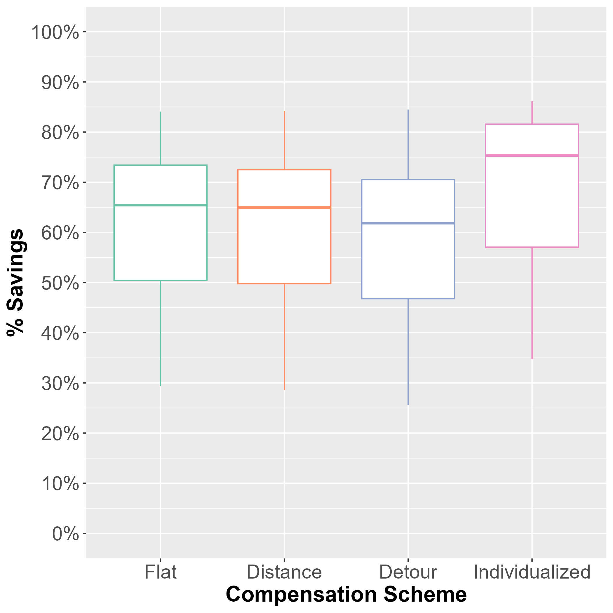
(a)

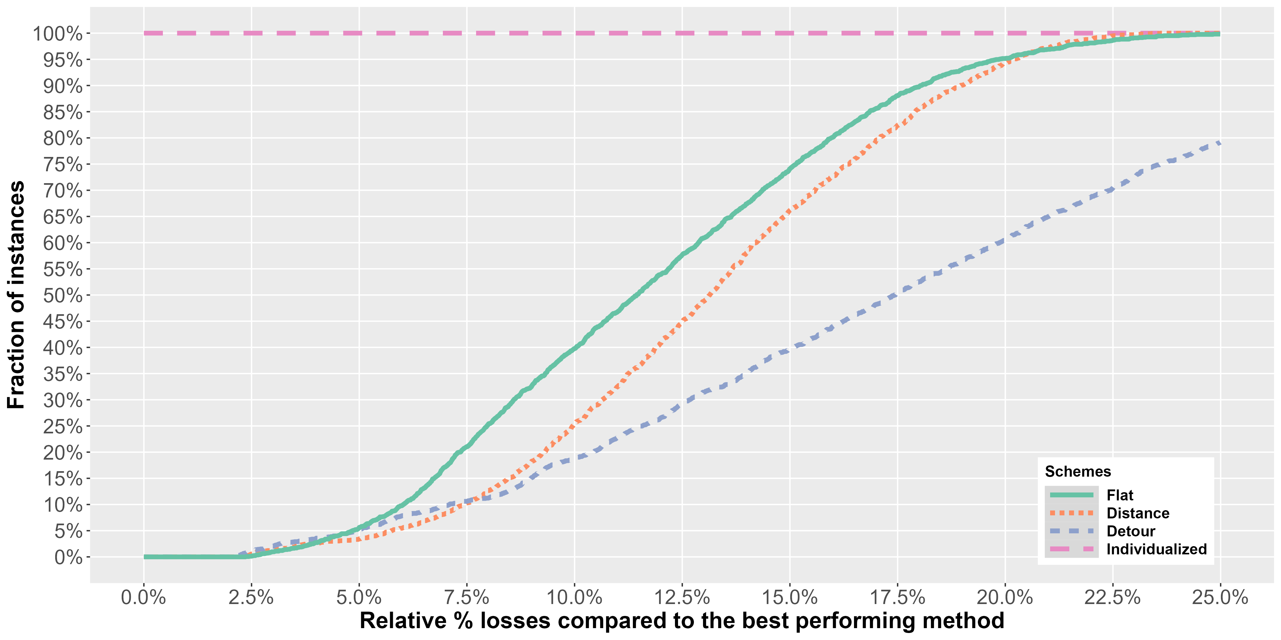
(b)

Figure 2: Expected total cost for linear acceptance probabilities.

First, we observe that the results obtained by using the individualized compensation scheme are strictly better than those of any other scheme in all instances considered. This follows because the relative loss of solution quality of the individualized scheme is zero in $100\%$ of the instances. For all other schemes, the relative loss is at least $2\%$ for each instance. Figure 2(b) also illustrates that the individualized scheme clearly outperforms all other schemes, that the flat scheme performs slightly better than the distance scheme, and that both of them clearly outperform the detour scheme. Note that this relative order of the schemes is rather unexpected. Intuitively, one would expect the distance and detour schemes to outperform the flat scheme, since the detour and distance amounts directly affect the acceptance probabilities. The results show that for each experimental configuration, the intervals of the relative mean difference in expected total cost between the individualized and benchmarks schemes are $(4.32\%,79.51\%)$, $(6.10\%,61.28\%)$, and $(5.02\%,66.78\%)$ for the detour, distance, and flat schemes, respectively. Paired t-tests confirm that the differences between the compensation schemes are statistically significant in all instances.

Mean acceptance rate

Figure 3(a) shows the fractions of tasks offered to occasional drivers by the different compensation schemes, while Figure 3(b) shows the mean acceptance rates of these tasks per instance. We observe that all schemes offer the majority of tasks to occasional drivers while achieving high expected acceptance rates. As for the previous two criteria, the individualized compensation scheme clearly outperforms the benchmark schemes as it achieves a higher acceptance rate while simultaneously offering more tasks. Among the benchmark schemes, the flat scheme shows the best performance, followed by the detour and distance schemes. The average differences in mean acceptance rates between the individualized and the benchmark schemes per experimental configuration take values in $(0.88\%,8.10\%)$, $(1.18\%,16.04\%)$ and $(1.24\%,8.10\%)$ for the detour, distance, and flat schemes, respectively. While the differences between the individualized scheme and the distance or flat scheme are statistically significant in all instances, this is not true for 49 out of 330 cases when comparing the individualized scheme and the detour scheme. These exceptions arise for instances with a relatively small number of occasional drivers, i.e., when $|J|\in\{50,75\}$. As their availability increases, the differences between the two schemes increase.

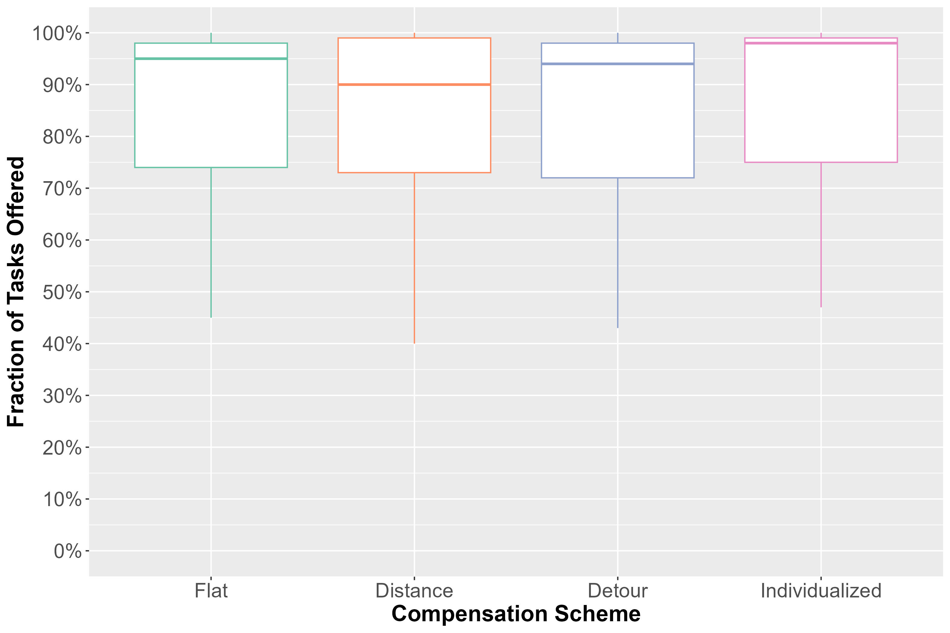
(a)

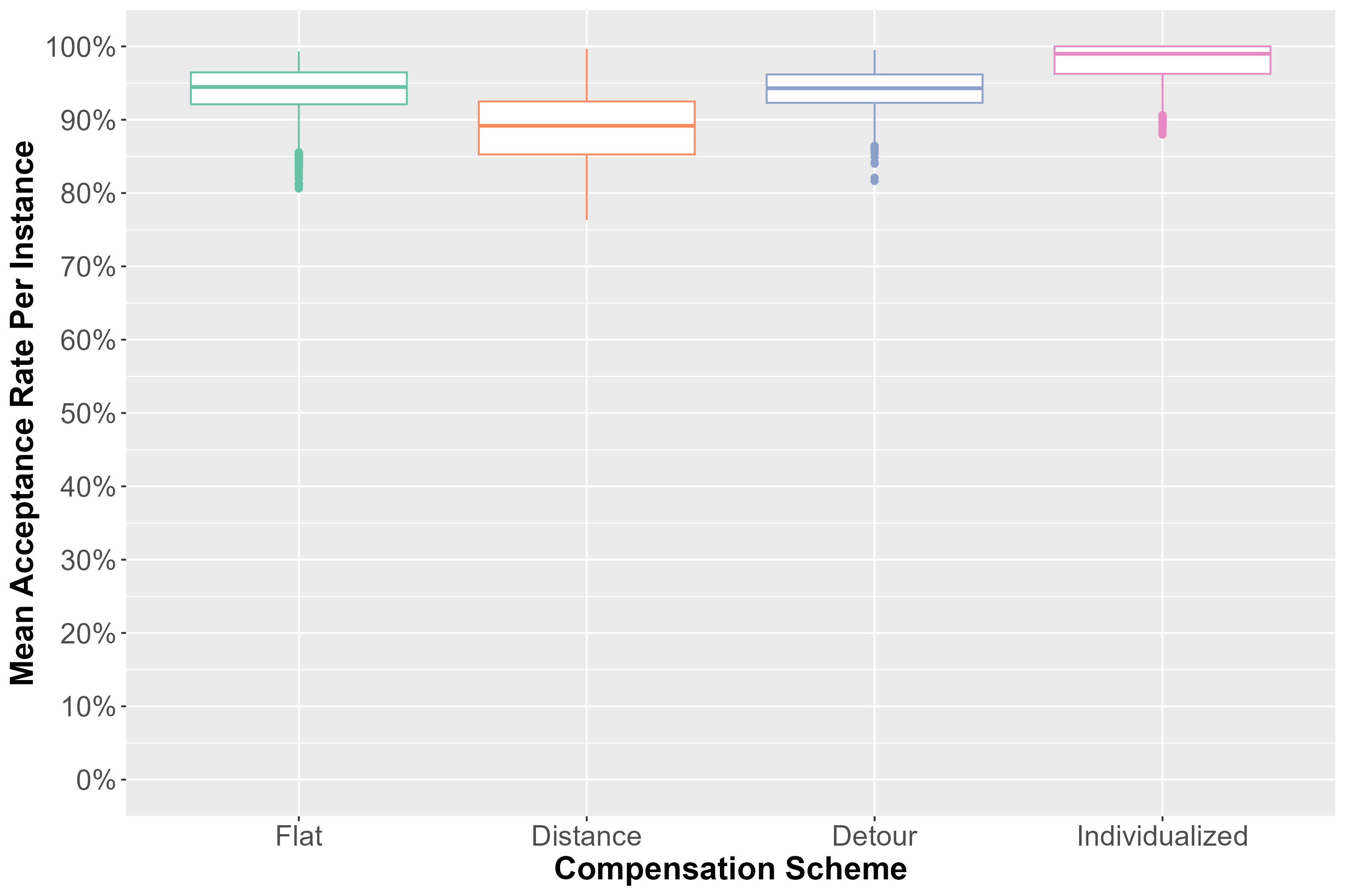
(b)

Figure 3: Fractions of offered tasks and expected acceptance rates for linear acceptance probabilities.

Overall, we conclude that the individualized scheme clearly outperforms all alternatives considered in each evaluation criteria. Thus, the use of the individualized scheme has the greatest potential to increase the satisfaction of occasional drivers and to reduce the use of professional drivers, while simultaneously reducing the expected total cost.

7.2 Performance comparison for logistic acceptance probabilities

Expected total cost

Figure 4(a) shows the relative cost savings of all four compensation schemes compared to the setting with no occasional drivers for logistic acceptance probability functions. Consistent with the case of the linear acceptance function, the individualized compensation scheme outperforms all benchmark schemes with median cost savings of more than $35\%$. Figure 4(b) shows that the individualized scheme outperforms all other schemes in every instance. For each parameter combination, the mean differences between the individualized scheme and the detour-based, distance-based, and flat schemes take values in the intervals $(0.27\%,6.73\%)$, $(1.31\%,8.99\%)$ and $(1.41\%,13.60\%)$, respectively. The statistical significance of the differences between the individualized and the benchmark schemes is confirmed for each setting considered by paired t-tests. Figure 4 also reveals that the detour-based scheme comes closest to the individualized scheme and outperforms the other two schemes. The flat compensation scheme shows the worst performance, which is in contrast to the case of linear acceptance probability functions, where the performance order of the three benchmark schemes is reversed.

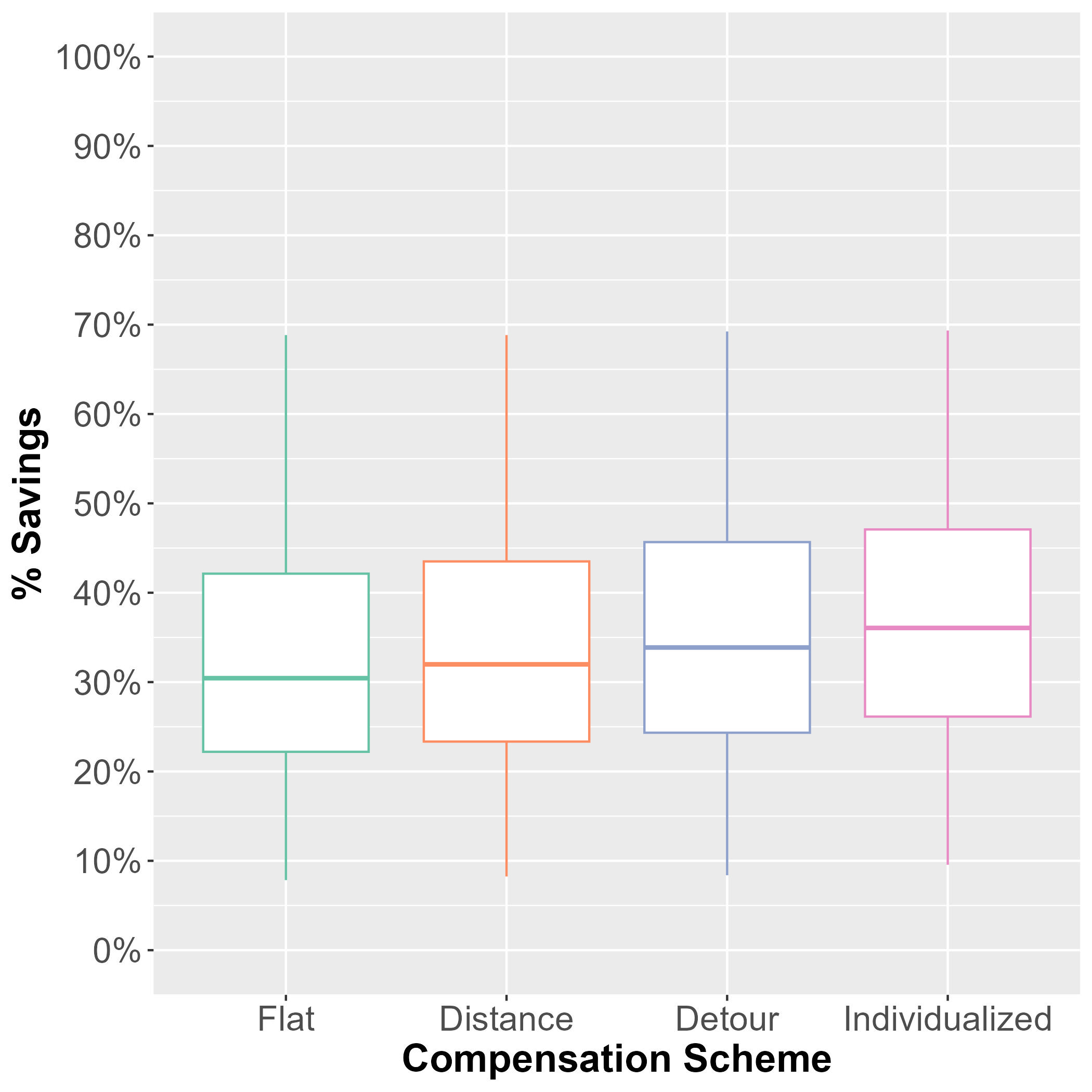
(a)

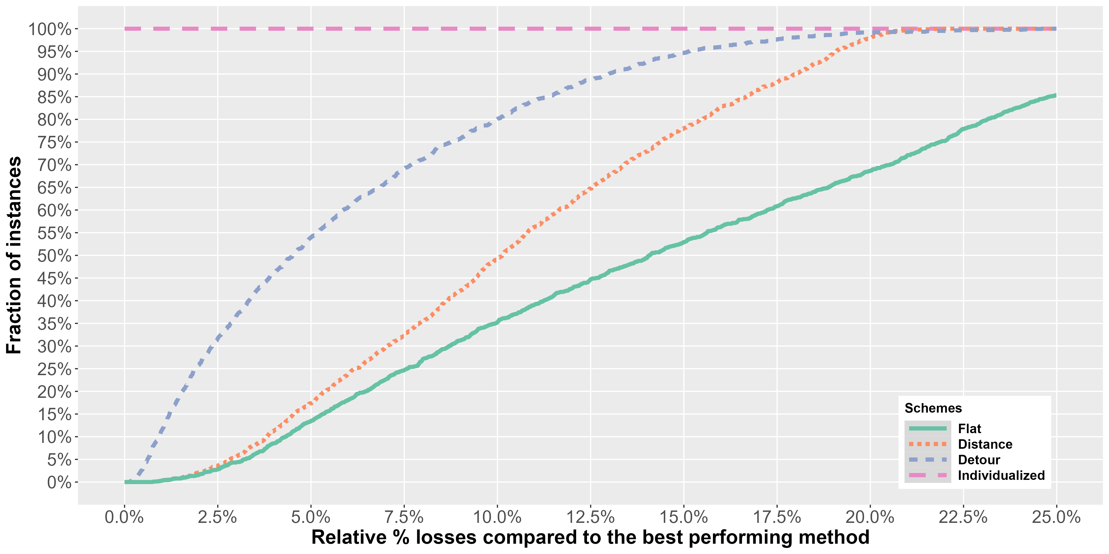
(b)

Figure 4: Expected total cost for logistic acceptance probabilities.

Mean acceptance rate

Figures 5(a) and 5(b) show that the individualized scheme is superior to the benchmark schemes, as it outsources more tasks than the other schemes and achieves the highest mean acceptance rate. The median fraction of tasks offered to occasional drivers is around $90\%$, and the median expected acceptance rate (per instance) of these offers is close to $70\%$. In comparison, the median fraction of tasks offered by the flat compensation scheme is only about $75\%$, and the median acceptance rate per instance is only slightly higher than $60\%$. If we examine the differences in each configuration, we see that the average differences of the mean acceptance rates per configuration of the detour, distance, and flat schemes to the individualized scheme lie in the intervals $(1.04\%,11.75\%)$, $(1.30\%,14.13\%)$, and $(3.11\%,24.68\%)$, respectively. While the differences between the individualized and the flat schemes are statistically significant in all cases, this is not true for the distance scheme in 2 out of $330$ configurations ($|J|=150$, $\rho\in\{20,50\}$, $\mu=0$) in which occasional drivers are mainly concerned with distance and are not sensitive to the detour. When comparing the detour-based and the individualized scheme, we observe that the differences are not statistically significant in $76$ out of $330$ configurations (in which $|J|\in\{50,75,100\}$). This shows that the individualized scheme significantly outperforms the detour-based schemes in environments characterized by an oversupply of occasional drivers.

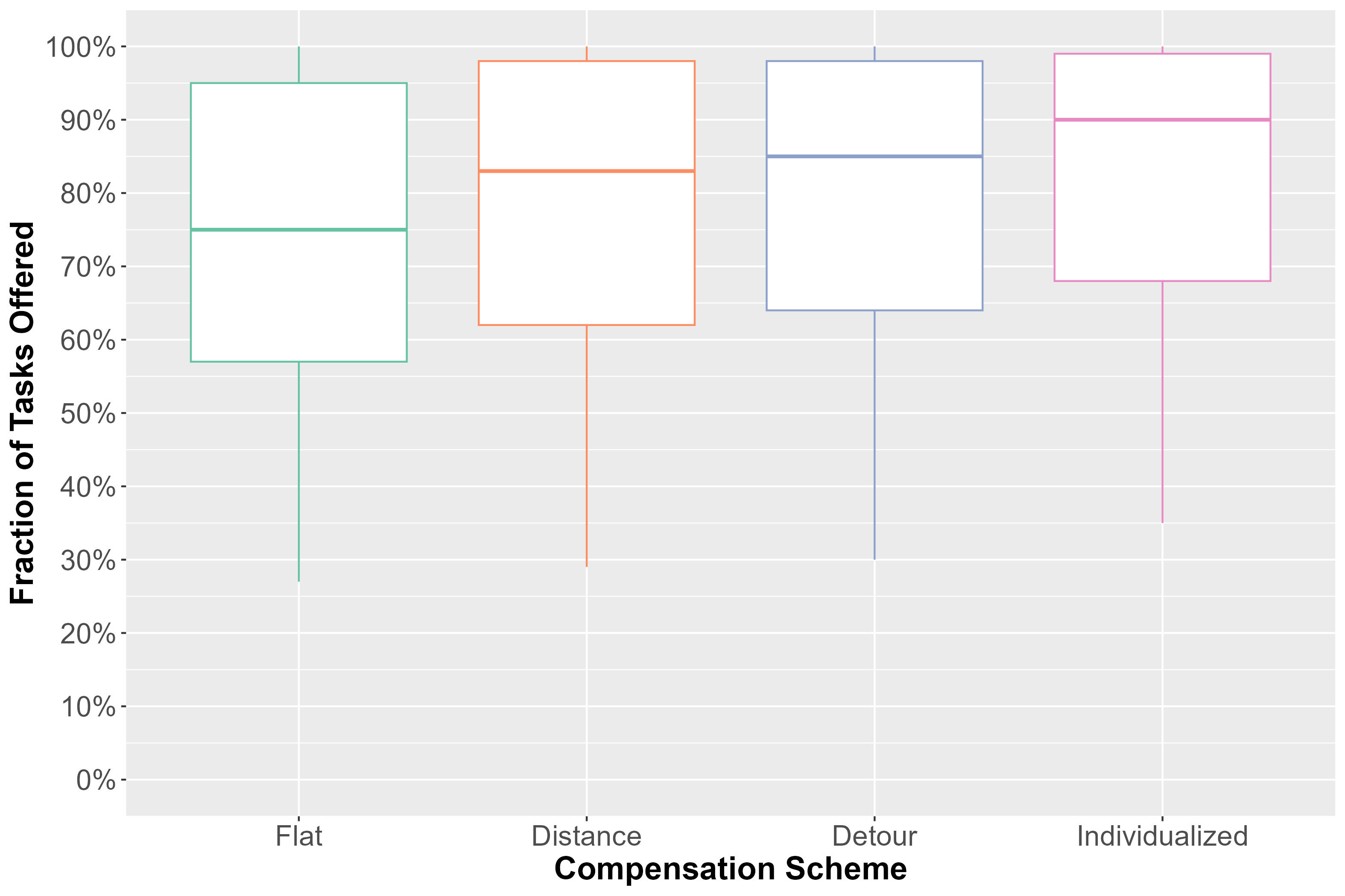
(a)

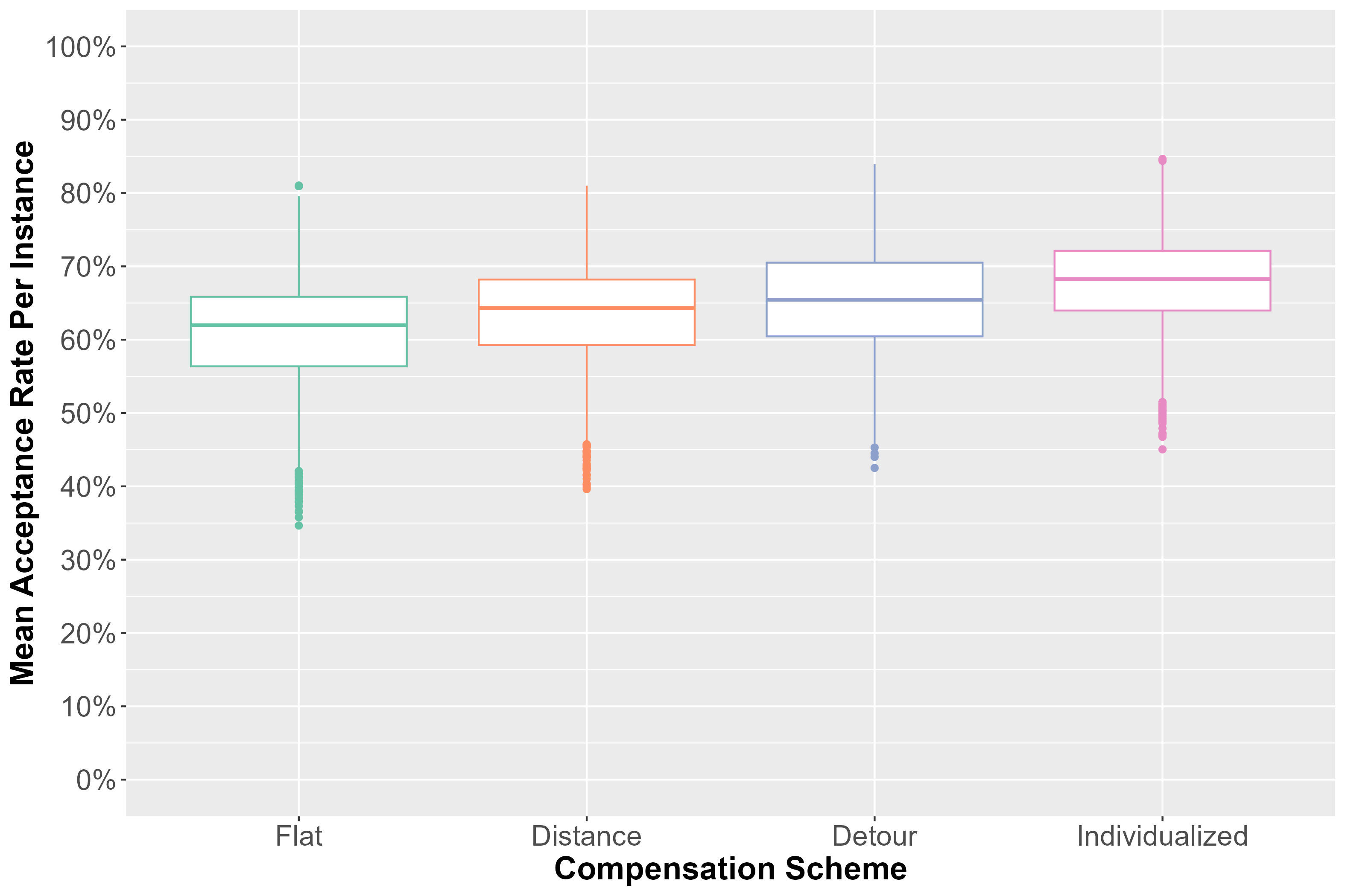
(b)

Figure 5: Fractions of offered tasks and expected acceptance rates for logistic acceptance probabilities.

Overall, we conclude that the individualized scheme clearly outperforms all alternatives considered in each evaluation criteria for both linear and logistic acceptance probability functions.

7.3 Sensitivity analysis

In the following, we analyze the sensitivity of the performance indicators with regard to changes in the availability of occasional drivers $|J|$, the penalty for rejected tasks $\rho$, and the parameter $\mu$ that affects the willingness to make detours. For the sake of brevity, and since all effects can be readily demonstrated within the logistic acceptance probability model, we restrict our discussion of sensitivity to the above parameters to that model. The full set of results can be found in the electronic companion.

Sensitivity towards availability of occasional drivers

Figure 6 shows the savings in expected total cost compared to the scenario with no occasional drivers, as well as the mean acceptance rates and fraction of tasks offered, respectively, for different numbers of (available) occasional drivers $|J|$. We observe that the savings tend to increase with increasing availability of occasional drivers for all the performance indicators, which is to be expected since a higher number gives the company more options to select cost-efficient occasional drivers. Figure 6(b) nicely illustrates that the number of tasks offered is always close to the maximum number possible (i.e., the minimum of $|I|$ and $|J$), while the mean acceptance always hovers around $65\%$. With a higher number of occasional drivers (i.e., with $|J|>|I|$), it is more likely to find occasional drivers who are more willing to accept the offers, and the mean acceptance increases (cf. Figure 6(c)).

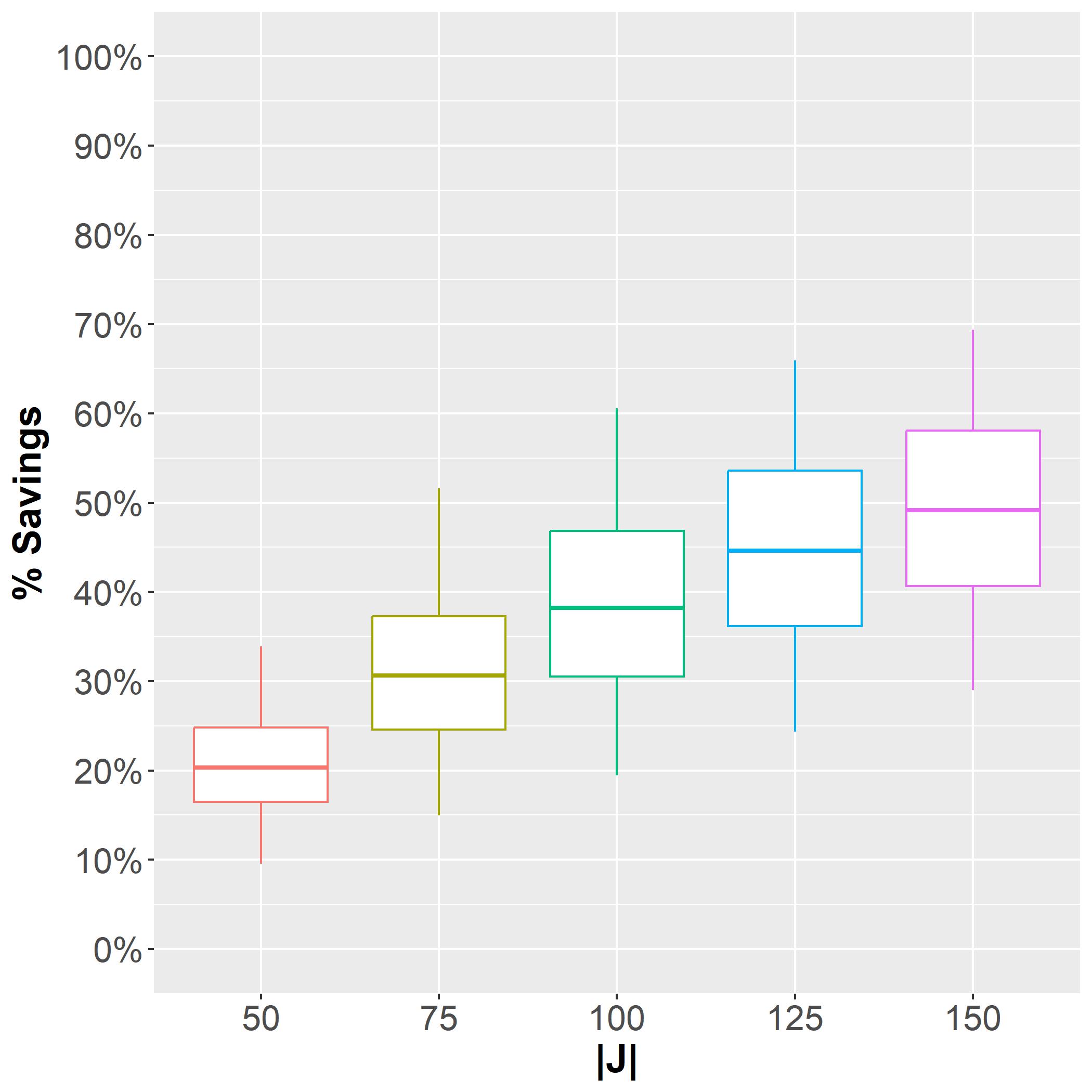
(a) Expected total cost.

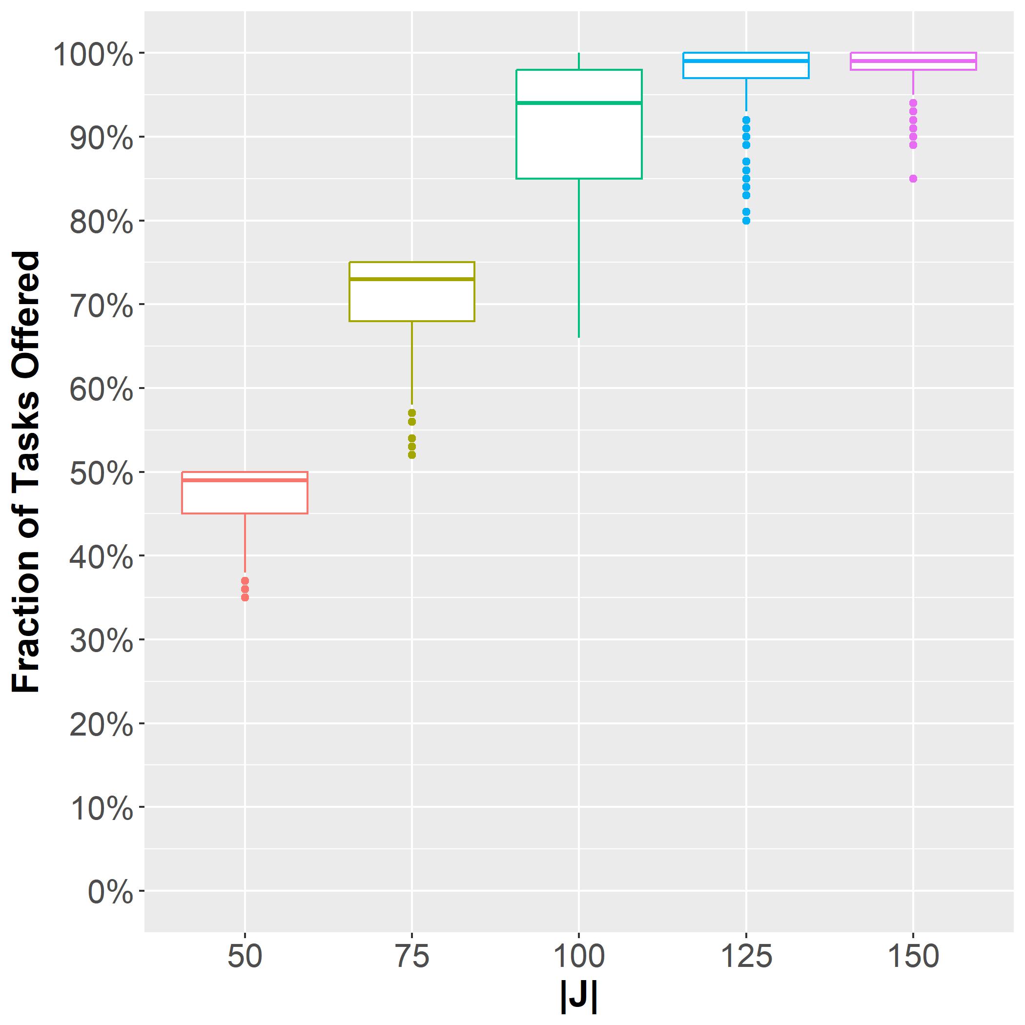
(b) Fraction of tasks offered.

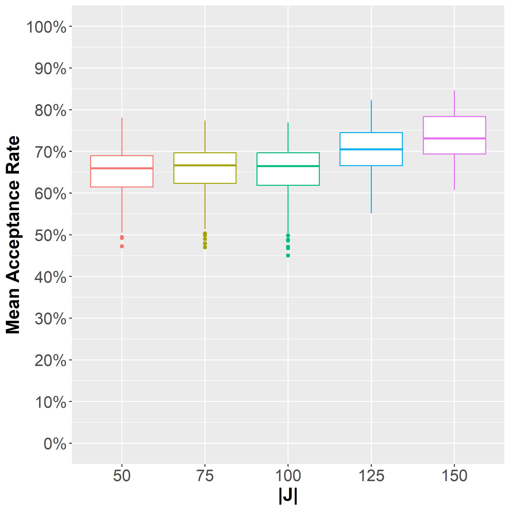
(c) Mean acceptance rate.

Figure 6: Sensitivity to availability

Sensitivity towards the penalty parameter $\rho$

Figure 7 illustrates the effect of increasing the penalty for rejected offers. As expected, an increase in the penalty has a significant impact on the individualized scheme, leading to fewer tasks being offered to the occasional drivers on average, cf. Figure 7(b). At the same time, the mean acceptance of offers increases (cf. Figure 7(c)), indicating a more careful selection of occasional drivers and a stronger focus on making good (acceptable) offers. The decrease in the number of occasional drivers used and the simultaneous increase in the penalty also lead to smaller savings in terms of total expected costs. However, as can be seen in Figure 7(a), the effects are much less severe than one would expect, decreasing from $40\%$ savings in the unrealistic case that no penalty is incurred to $33\%$ in the case that a rejected offer leads to a $25\%$ increase in operational costs. One explanation is that the individualized compensation scheme allows good (acceptable) offers to be made to occasional drivers for tasks that would initially be very costly to the company using professional drivers, thus allowing the company to efficiently outsource them to occasional drivers.

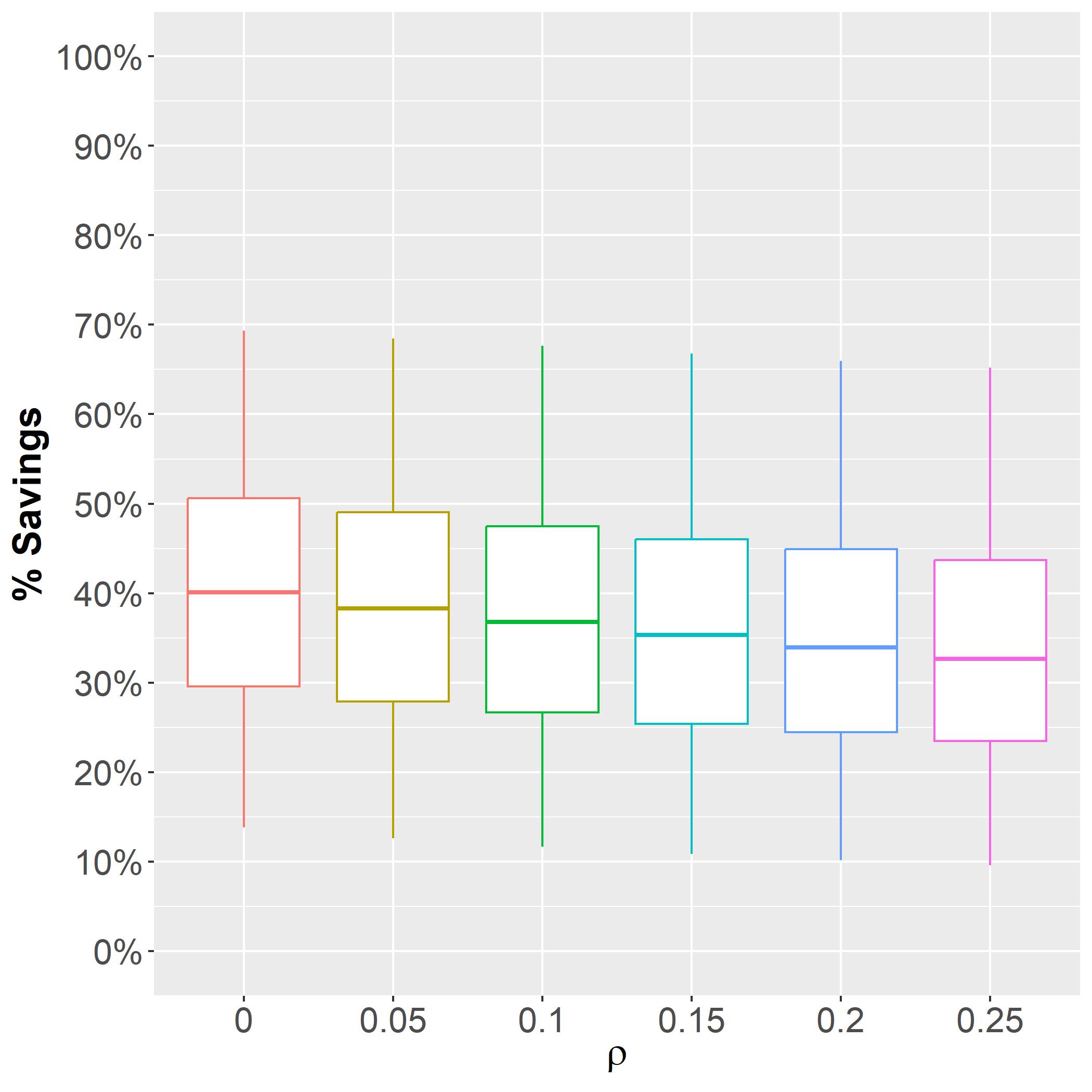
(a) Expected total cost.

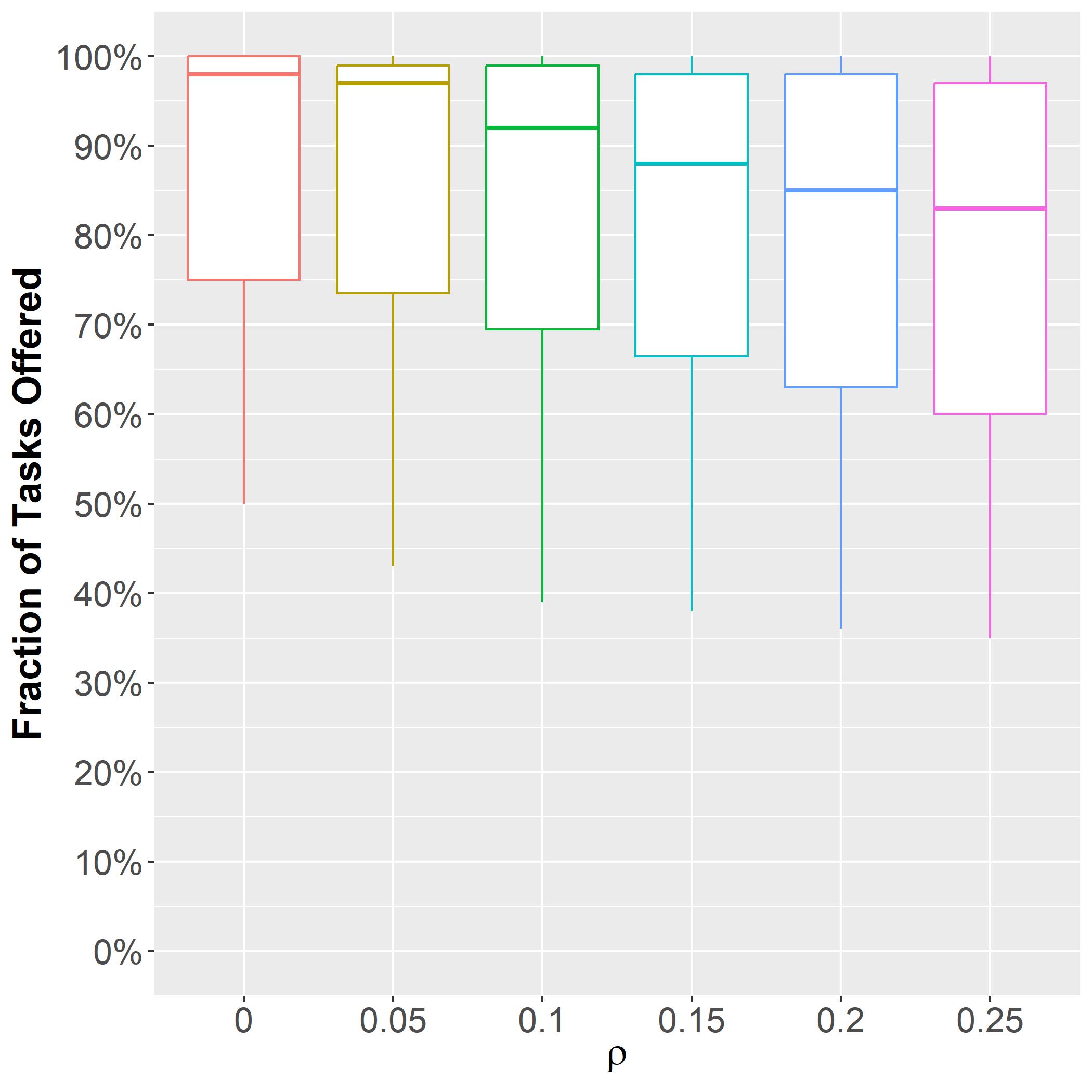
(b) Fraction of tasks offered.

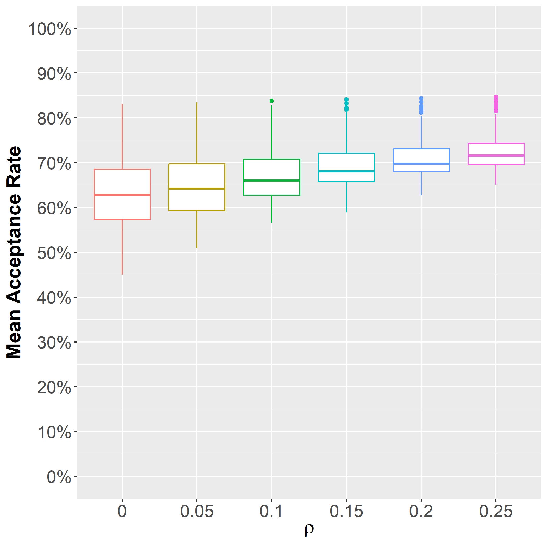
(c) Mean acceptance rate.

Figure 7: Sensitivity to penalty

Sensitivity towards parameter $\mu$

A larger value of $\mu$ increases the acceptance probability because it increases the willingness of occasional drivers to make a detour. As can be seen in Figure 8, this increases the savings in terms of expected total cost, more tasks are offered to occasional drivers, and the acceptance rates also increase, cf. Figures 8(a), 8(b) and 8(c). While this effect was expected, it is worth noting that the individualized scheme generates significant cost savings for all parameter values considered. Furthermore, high fractions of tasks offered to occasional drivers and mean acceptance rates indicate that it allows to outsource a high proportion of tasks to occasional drivers, relatively independent of the concrete value of parameter $\mu$.

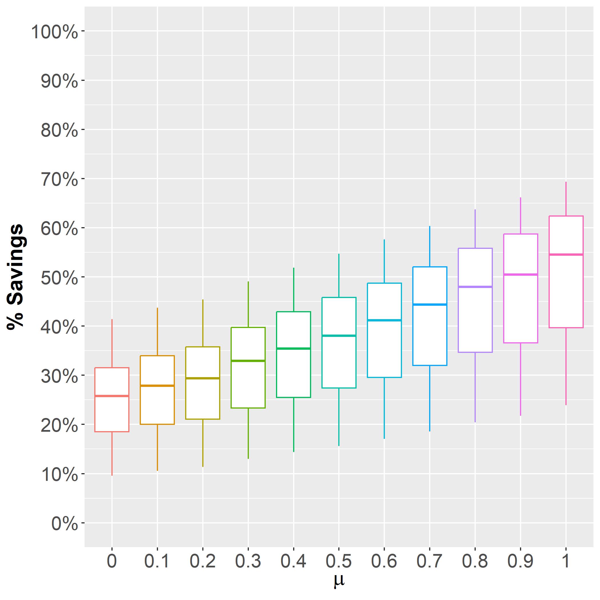
(a) Expected total cost.

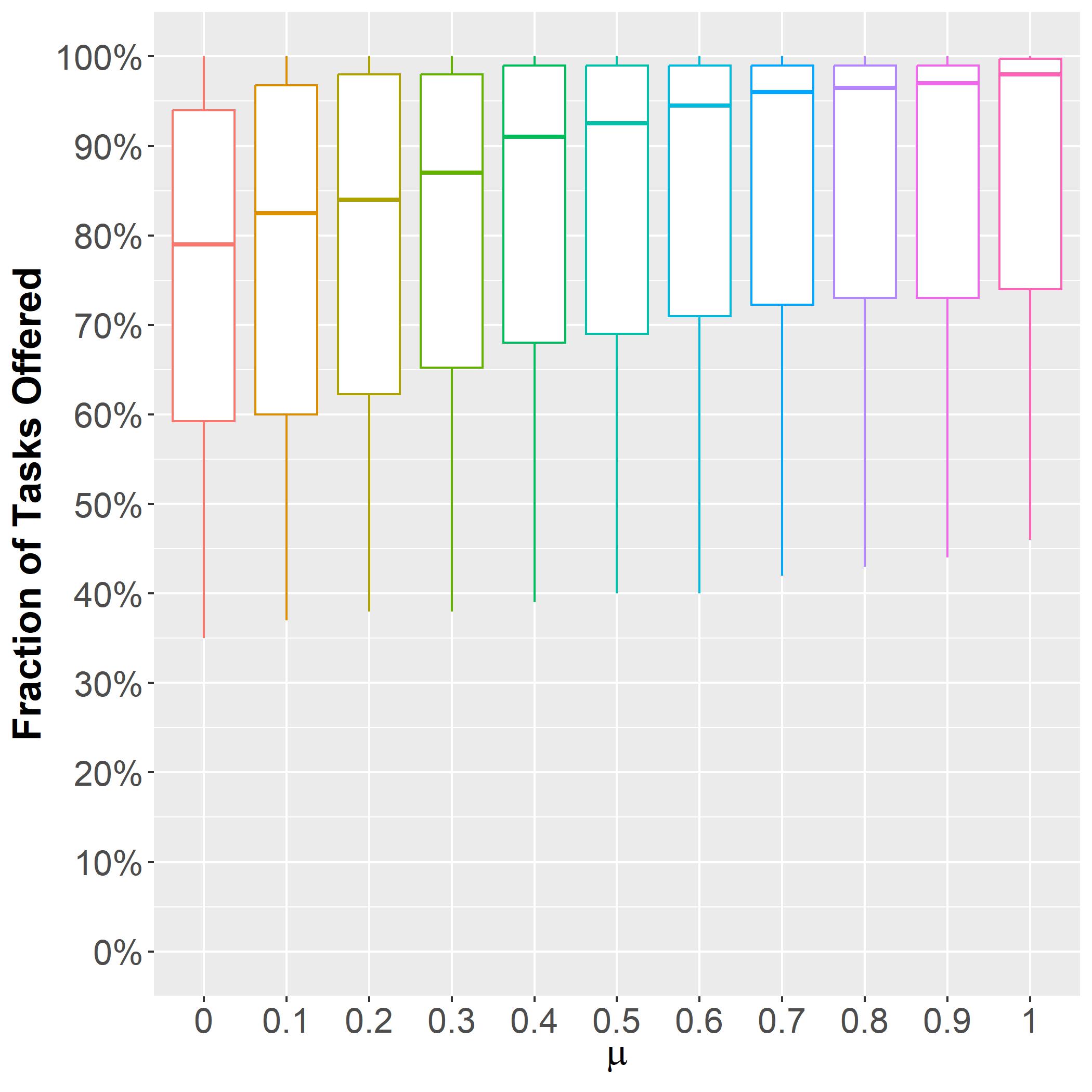
(b) Fraction of tasks offered.

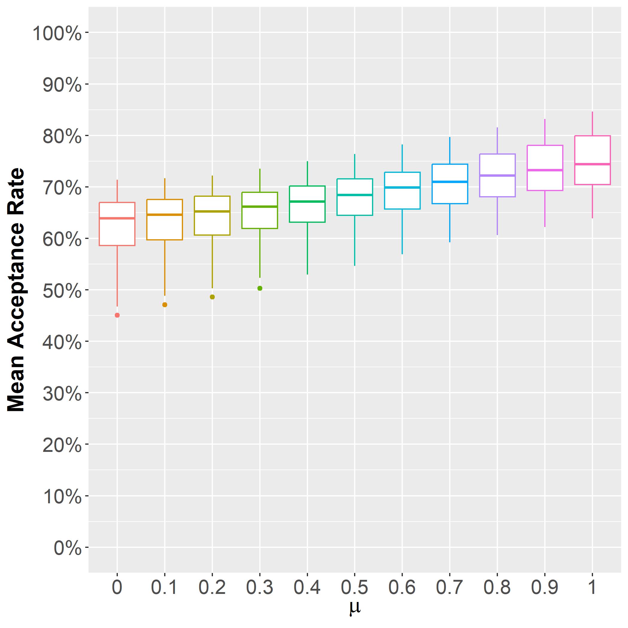
(c) Mean acceptance rate.

Figure 8: Sensitivity to distance utility weight

8 Conclusions and future work

In this paper, we introduced the Crowdshipping Assignment Problem with Compensation-Driven Acceptance Behavior which defines an integrated solution to the task assignment and compensation decisions, while explicitly accounting for the probability with which occasional drivers will accept these assignments. To this end, we proposed an MINLP formulation for generic acceptance probability functions and showed that it can be solved optimally with a two-stage approach that decomposes compensation and assignment decisions. Moreover, we proposed an exact linearization of our MINLP formulation and showed that the latter can be solved in polynomial time for generic probability functions under mild conditions. We also derived explicit formulas for optimal compensation decisions for linear and logistic acceptance probability functions which are two particularly relevant, special cases of our generic setting. Furthermore, we investigated the non-separable case where the decision-maker has additional restrictions on compensation and assignment decisions, and propose an approximate linearization for this extension.

We conducted an extensive computational study comparing our approach with established benchmark compensation schemes from the literature. The results of our study show that the use of crowdshippers can lead to substantial benefits and that our approach outperforms the compensation schemes from the literature in terms. Our model allows operators to offer individualized compensation that results in a very high rate of accepted offers while achieving higher cost savings than the other schemes, which is due to the flexibility of our model according to the results. This is an important observation from the perspective of both the operator and the occasional driver. It shows that more occasional drivers can be utilized, which may result in lower dependency on third party logistic companies or a dedicated private fleet to fulfill the tasks.Moreover, a high acceptance rate of offers shows that the offers are more persuasive to occasional drivers, which signals higher driver satisfaction and therefore may result in a higher engagement and availability of occasional drivers in the long run. The sensitivity analysis shows that the proposed model is robust with regard to variations in the availability of occasional drivers and adapts very well to changes in the magnitude of the penalty incurred for rejected offers as well as to changes in the utility functions of occasional drivers.

Future research can be devoted to studying dynamic versions of the problem, where tasks and available drivers are unknown in advance and become available over time. Given its efficiency, our approach could be embedded in an approximate dynamic programming framework to take compensation decisions at each time step while acceptance probabilities could be dynamically updated according to the earlier decisions taken by occasional drivers. Another possible avenue is to enrich the problem by considering additional features such as routing decisions and offering bundles of tasks to occasional drivers.

Appendix A Proofs

Proof of Theorem 1..

We conclude that the second statement of the theorem holds since compensation values $C_{ij}$ are irrelevant if task $i\in I$ is not offered to occasional driver $j\in J$, cf. objective function (1). Assume that task $i\in I$ is offered to occasional driver $j\in J$. We observe that an optimal compensation value $C_{ij}^{*}$ is equal to

$$C_{ij}^{*}=\mathrm{argmin}_{C_{ij}\geq 0}P_{ij}(C_{ij})(C_{ij}-c^{\prime}_{i})+c_{i}^{\prime}$$

since this value minimizes the (relevant terms of) objective function (2) and there are no dependencies on other tasks and drivers. The theorem follows because the last term of this equation is constant and can therefore be neglected. ∎

Proof of Proposition 1..

Recall that the optimal compensation values are calculated according to Equation (7) given in Corollary 1. We observe that the minimum of Equation (7) when plugging in probability function (10) is attained for $C_{ij}\in]0,c_{i}^{\prime}]$, in which case its value is less than or equal to zero, while it is equal to zero if $C_{ij}=0$. Similarly, we have $C_{ij}\leq\frac{1-\alpha_{ij}}{\beta_{ij}}$ since $P_{ij}(\frac{1-\alpha_{ij}}{\beta_{ij}})=1$ and further increasing the compensation would increase the value of $P_{ij}(C_{ij})(C_{ij}-c_{i}^{\prime})$. Thus, an optimal compensation value for task $i\in I$ when offered to occasional driver $j\in J$ must be a minimizer of $(\alpha_{ij}+\beta_{ij}C_{ij})(C_{ij}-c_{i}^{\prime})=\beta_{ij}C_{ij}^{2}+(\alpha_{ij}-\beta_{ij}c_{i}^{\prime})C_{ij}-\alpha_{ij}c_{i}^{\prime}$. By taking the first derivative (and since the second derivative is non-negative), the minimizer $C_{ij}^{*}$ is obtained as

$$2\beta_{ij}C_{ij}^{*}+\alpha_{ij}-\beta_{ij}c_{i}^{\prime}=0\Leftrightarrow C_{ij}^{*}=\frac{c_{i}^{\prime}}{2}-\frac{\alpha_{ij}}{2\beta_{ij}}.$$

∎

Proof of Proposition 2..

We first observe that optimal compensation values lie in the intervals $]0,c_{i}^{\prime}]$ since Equation (7) evaluates to a non-positive value in this interval. Thus, an optimal compensation value for task $i\in I$ when offered to occasional driver $j\in J$ must be a minimizer of $\frac{C_{ij}-c_{i}^{\prime}}{1+e^{-(\gamma_{ij}+\delta_{ij}C_{ij})}}$ whose first derivative $\frac{e^{-(\gamma_{ij}+\delta_{ij}C_{ij})}\left(1+(C_{ij}-c_{i}^{\prime})\delta_{ij}+e^{\gamma_{ij}+\delta_{ij}C_{ij}}\right)}{\left(1+e^{-(\gamma_{ij}+\delta_{ij}C_{ij})}\right)^{2}}$ is equal to zero if and only if the (strictly monotonically increasing) function $1+(C_{ij}-c_{i}^{\prime})\delta_{ij}+e^{\gamma_{ij}+\delta_{ij}C_{ij}}$ is equal to zero. We use the following basic manipulations

$$1+(C_{ij}^{*}-c_{i}^{\prime})\delta_{ij}+e^{\gamma_{ij}+\delta_{ij}C_{ij}^{*}}=0 \quad\Leftrightarrow\quad e^{\gamma_{ij}+\delta_{ij}C_{ij}^{*}}=c_{i}^{\prime}\delta_{ij}-1-\delta_{ij}C_{ij}^{*}\quad\Leftrightarrow$$

$$\Leftrightarrow\quad(c_{i}^{\prime}\delta_{ij}-1-\delta_{ij}C_{ij}^{*})e^{-\gamma_{ij}-\delta_{ij}C_{ij}^{*}}=1 \quad\Leftrightarrow\quad(c_{i}^{\prime}\delta_{ij}-1-\delta_{ij}C_{ij}^{*})e^{c_{i}^{\prime}\delta_{ij}-1-\delta_{ij}C_{ij}^{*}}=e^{\gamma_{ij}+c_{i}^{\prime}\delta_{ij}-1}$$

that hold for optimal compensation values $C_{ij}^{*}$ and observe that the last equation has the form $ze^{z}=b$ for $z=c_{i}^{\prime}\delta_{ij}-1-\delta_{ij}C_{ij}^{*}$ and $b=e^{\gamma_{ij}+c_{i}^{\prime}\delta_{ij}-1}$. It can therefore be solved using the real-valued Lambert $W$ function $W(ze^{z})=z$ and it follows that

$$c_{i}^{\prime}\delta_{ij}-1-\delta_{ij}C_{ij}^{*} =W(e^{\gamma_{ij}+c_{i}^{\prime}\delta_{ij}-1}) \quad\Leftrightarrow\quad C_{ij}^{*}=-\frac{W(e^{\gamma_{ij}+c_{i}^{\prime}\delta_{ij}-1})-c_{i}^{\prime}\delta_{ij}+1}{\delta_{ij}}.$$

∎

Proof of Proposition 3..

Obviously, the problem is in NP, since any assignment and compliance with the constraints can be verified in polynomial time (given there is only a polynomial number of constraints of type (12)). We show the proposition by reduction from the multidimensional knapsack problem. Let $A$ be an instance of the multidimensional knapsack problem with $d$ dimensions and items $I^{K}$ with value $v^{K}_{i}$ for $i^{K}\in I^{K}$. Let $C^{K}_{\ell}$ be the capacity of the knapsack in dimension $\ell=1,\ldots,d$ and $w^{K}_{i\ell}$ be the weight of $i^{K}\in I^{K}$ in dimension $\ell=1,\ldots,d$. Design an instance $A^{\prime}$ of CAPCABwS with tasks $I$ as follows:

• Let $\omega=\Pi_{i\in I^{K}}\min\left\{v_{i^{K}},2\right\}$ be a large constant.

• With each item $i^{K}\in I^{K}$ identify a task $i\in I$ with $c_{i}=c^{\prime}_{i}=\omega v^{K}_{i}$.

• Let $J$ be the set of occasional drivers with $|J|\geq|I|$. For each $j\in J$ set the parameters of the probability function such that $j$ accepts a task $i\in I$ for any $C_{ij}>0$.

• For $\ell=1,\ldots,d$ introduce the non-separability constraint

  $$\sum_{i\in I}\sum_{j\in J}(w^{K}_{i\ell}x_{ij})\leq C^{K}_{\ell}.$$ (15)

Each constraint (15) in $A^{\prime}$ models the knapsack constraint for dimension $\ell$ in $A$. Then, there exists a solution to $A$ with a value of at least $V$ if and only if there exists an assignment of tasks in $A^{\prime}$ with an expected cost of at most $\tilde{C}=\left(\sum_{i^{k}\in I^{K}}v_{i^{k}}-V\right)\omega+1$.

• Let $i_{1}^{K},\ldots,i_{n}^{K}$ be a feasible solution for $A$ with $V=\sum_{1}^{n}v^{K}_{i}$, which are identified by tasks $1,\ldots,n$ in $A^{\prime}$. Take $n$ occasional drivers in $J$, w.l.o.g. $1,\ldots,n$ and offer a compensation of $C_{ij}=\frac{1}{n}$. The construction of the probability function ensures that the occasional drivers will accept these tasks (with a probability of one). Due to the construction of the non-separability constraints, and since the solution is feasible for the $A$, assigning the tasks to these occasional drivers is also feasible in $A^{\prime}$. Since no other tasks are offered to the occasional drivers, the total expected cost is $\tilde{C}$.

• Consider a feasible solution to $A^{\prime}$ with cost of $C^{\prime}\leq\tilde{C}$ in which, w.l.o.g., tasks $1,\ldots,n$ are allocated to occasional drivers. Since the occasional drivers require a compensation strictly greater than zero to perform the task, it holds that

  $$\sum_{j\in J}\sum_{i\in J}v^{K}_{i}x_{ij}\geq V$$

  since otherwise the total expected cost would be higher than $\tilde{C}$. Then, the corresponding items $i^{K}_{1},\ldots,i^{K}_{n}$ also sum up to a value of at least $V$ in $A$. Since all non-separability constraints are adhered to in $A^{\prime}$, this solution is also feasible for $A$.

∎

Proof of Proposition 4..

We first recall that $x_{ij}=0$ implies $C_{ij}=0$ due to inequalities (2d). Since $P_{ij}(0)=0$ holds by assumption all nonlinear terms, $P_{ij}(C_{ij})x_{ij}$ in objective function (2a) can be replaced by $P_{ij}(C_{ij})$. As a consequence the proposition follows since

$$\sum_{i\in I}c_{i}y_{i}+\sum_{i\in I}\sum_{j\in J}\left(P_{ij}(C_{ij})C_{ij}+(1-P_{ij}(C_{ij}))c_{i}^{\prime}\right)x_{ij}=$$

$$= \sum_{i\in I}c_{i}y_{i}+\sum_{i\in I}\sum_{j\in J}\left(C_{ij}P_{ij}(C_{ij})x_{ij}-c_{i}^{\prime}P_{ij}(C_{ij})x_{ij}+c_{i}^{\prime}x_{ij}\right)=$$

$$= \sum_{i\in I}c_{i}y_{i}+\sum_{i\in I}\sum_{j\in J}\left(P_{ij}(C_{ij})(C_{ij}-c_{i}^{\prime})+c_{i}^{\prime}x_{ij}\right)$$

∎

Proof of Proposition 5..

Using $U_{ij}=\min\{c_{i},\frac{1-\alpha_{ij}}{\beta_{ij}}\}$ discussed in Section 3.2, the linear acceptance probability function (3) can be simplified to $P_{ij}(C_{ij})=\alpha_{ij}+\beta_{ij}C_{ij}$ due to constraints (2d), cf. Proposition 4. Thus, $f_{ij}(C_{ij})+g_{ij}(x_{ij})$ must be equal to the corresponding (nonlinear) part of (4) for each $i\in I$ and $j\in J$ and we have

$$f_{ij}(C_{ij})+g_{ij}(x_{ij}) =(P_{ij}(C_{ij})C_{ij}+(1-P_{ij}(C_{ij}))c_{i}^{\prime})x_{ij}=$$

$$=((\alpha_{ij}+\beta_{ij}C_{ij})C_{ij}+(1-\alpha_{ij}-\beta_{ij}C_{ij})c^{\prime}_{i})x_{ij}=$$

$$=\beta_{ij}C_{ij}^{2}x_{ij}+(\alpha_{ij}-\beta_{ij}c_{i}^{\prime}C_{ij}x_{ij}+c_{i}^{\prime}(1-\alpha_{ij})x_{ij}=$$

$$=\underbrace{\beta_{ij}C_{ij}^{2}+(\alpha_{ij}-\beta_{ij}c_{i}^{\prime})C_{ij}}_{f_{ij}(C_{ij})}+\underbrace{c_{i}^{\prime}(1-\alpha_{ij})x_{ij}}_{g_{ij}(x_{ij})}$$

The last equation holds since $x_{ij}=0$ implies that $C_{ij}=0$ due to constraints (2d). The second part of the proposition follows since $f_{ij}(C_{ij})$ is a convex (quadratic) function as $\beta_{ij}>0$. ∎

Proof of Proposition 6..

We first observe that the proposition holds for $C_{ij}=0$ in which case we obtain $f_{ij}(C_{ij})+g_{ij}(x_{ij})=c_{i}^{\prime}x_{ij}$. For $0<C_{ij}\leq U_{ij}$ we obtain

$$f_{ij}(C_{ij})+g_{ij}(x_{ij}) =(P_{ij}(C_{ij})C_{ij}+(1-P_{ij}(C_{ij}))c_{i}^{\prime})x_{ij}=\frac{(C_{ij}-c_{i}^{\prime})x_{ij}}{1+e^{-\gamma_{ij}-\delta_{ij}C_{ij}}}+c_{i}^{\prime}x_{ij}.$$

We observe that we can remove $x_{ij}$ from $(C_{ij}-c_{i}^{\prime})x_{ij}$ since the assumption $C_{ij}>0$ implies that $x_{ij}=1$. ∎

Appendix B Additional and detailed computational results

Table 2: Paired t-test results comparing the individualized compensation scheme with the benchmark schemes in terms of total expected cost obtained using linear acceptance probability.

$|J|$	$\rho$	$\mu$	Individualized	Detour		Distance		Flat
				$\%$ Diff.	p-Val	$\%$ Diff.	p- Val	$\%$ Diff.	p-Val
50	0.00	0.00	4617.53	0.15	0.00	0.08	0.00	0.08	0.00
		0.10	4573.57	0.14	0.00	0.08	0.00	0.08	0.00
		0.20	4526.51	0.13	0.00	0.08	0.00	0.08	0.00
		0.30	4476.96	0.12	0.00	0.08	0.00	0.08	0.00
		0.40	4424.89	0.12	0.00	0.07	0.00	0.07	0.00
		0.50	4370.55	0.11	0.00	0.07	0.00	0.07	0.00
		0.60	4311.78	0.10	0.00	0.07	0.00	0.06	0.00
		0.70	4248.36	0.09	0.00	0.07	0.00	0.06	0.00
		0.80	4180.39	0.08	0.00	0.06	0.00	0.06	0.00
		0.90	4107.25	0.07	0.00	0.06	0.00	0.05	0.00
		1.00	4031.02	0.04	0.00	0.06	0.00	0.05	0.00
	0.05	0.00	4638.81	0.14	0.00	0.09	0.00	0.08	0.00
		0.10	4594.34	0.14	0.00	0.09	0.00	0.08	0.00
		0.20	4546.85	0.13	0.00	0.09	0.00	0.08	0.00
		0.30	4496.62	0.12	0.00	0.08	0.00	0.08	0.00
		0.40	4444.26	0.11	0.00	0.08	0.00	0.07	0.00
		0.50	4389.67	0.11	0.00	0.08	0.00	0.07	0.00
		0.60	4330.36	0.10	0.00	0.07	0.00	0.07	0.00
		0.70	4266.70	0.09	0.00	0.07	0.00	0.06	0.00
		0.80	4197.91	0.08	0.00	0.07	0.00	0.06	0.00
		0.90	4123.62	0.07	0.00	0.07	0.00	0.05	0.00
		1.00	4046.93	0.04	0.00	0.06	0.00	0.05	0.00
	0.10	0.00	4655.59	0.14	0.00	0.09	0.00	0.08	0.00
		0.10	4611.02	0.14	0.00	0.09	0.00	0.08	0.00
		0.20	4563.27	0.13	0.00	0.09	0.00	0.08	0.00
		0.30	4512.21	0.12	0.00	0.09	0.00	0.08	0.00
		0.40	4458.82	0.11	0.00	0.08	0.00	0.07	0.00
		0.50	4403.55	0.11	0.00	0.08	0.00	0.07	0.00
		0.60	4343.94	0.10	0.00	0.08	0.00	0.07	0.00
		0.70	4279.69	0.09	0.00	0.07	0.00	0.06	0.00
		0.80	4210.03	0.08	0.00	0.07	0.00	0.06	0.00
		0.90	4135.38	0.07	0.00	0.07	0.00	0.05	0.00
		1.00	4058.26	0.04	0.00	0.07	0.00	0.05	0.00
	0.15	0.00	4665.98	0.14	0.00	0.10	0.00	0.08	0.00
		0.10	4621.43	0.14	0.00	0.10	0.00	0.08	0.00
		0.20	4573.72	0.13	0.00	0.09	0.00	0.08	0.00
		0.30	4521.90	0.12	0.00	0.09	0.00	0.08	0.00
		0.40	4468.45	0.11	0.00	0.09	0.00	0.07	0.00
		0.50	4412.85	0.11	0.00	0.08	0.00	0.07	0.00
		0.60	4352.55	0.10	0.00	0.08	0.00	0.07	0.00
		0.70	4288.43	0.09	0.00	0.08	0.00	0.06	0.00
		0.80	4218.11	0.08	0.00	0.07	0.00	0.06	0.00
		0.90	4143.48	0.07	0.00	0.07	0.00	0.06	0.00
		1.00	4065.98	0.05	0.00	0.07	0.00	0.05	0.00
	0.20	0.00	4672.25	0.14	0.00	0.10	0.00	0.09	0.00
		0.10	4627.93	0.14	0.00	0.10	0.00	0.08	0.00
		0.20	4580.41	0.13	0.00	0.10	0.00	0.08	0.00
		0.30	4528.96	0.12	0.00	0.09	0.00	0.08	0.00
		0.40	4475.72	0.12	0.00	0.09	0.00	0.08	0.00
		0.50	4419.85	0.11	0.00	0.09	0.00	0.07	0.00
		0.60	4359.04	0.10	0.00	0.08	0.00	0.07	0.00
		0.70	4294.91	0.09	0.00	0.08	0.00	0.06	0.00
		0.80	4224.54	0.08	0.00	0.08	0.00	0.06	0.00
		0.90	4149.98	0.07	0.00	0.07	0.00	0.06	0.00
		1.00	4071.96	0.05	0.00	0.07	0.00	0.05	0.00
	0.25	0.00	4675.80	0.14	0.00	0.10	0.00	0.09	0.00
		0.10	4631.57	0.14	0.00	0.10	0.00	0.08	0.00
		0.20	4583.88	0.13	0.00	0.10	0.00	0.08	0.00
		0.30	4532.59	0.13	0.00	0.10	0.00	0.08	0.00
		0.40	4479.37	0.12	0.00	0.09	0.00	0.08	0.00
		0.50	4423.57	0.11	0.00	0.09	0.00	0.07	0.00
		0.60	4362.62	0.10	0.00	0.09	0.00	0.07	0.00
		0.70	4298.55	0.09	0.00	0.08	0.00	0.06	0.00
		0.80	4228.30	0.08	0.00	0.08	0.00	0.06	0.00
		0.90	4153.63	0.07	0.00	0.08	0.00	0.06	0.00
		1.00	4075.62	0.05	0.00	0.07	0.00	0.05	0.00
75	0.00	0.00	3211.97	0.31	0.00	0.19	0.00	0.19	0.00
		0.10	3150.19	0.30	0.00	0.18	0.00	0.18	0.00
		0.20	3085.64	0.29	0.00	0.18	0.00	0.18	0.00
		0.30	3018.23	0.27	0.00	0.17	0.00	0.17	0.00
		0.40	2946.62	0.26	0.00	0.17	0.00	0.16	0.00
		0.50	2872.59	0.24	0.00	0.17	0.00	0.15	0.00
		0.60	2794.91	0.23	0.00	0.16	0.00	0.15	0.00
		0.70	2711.08	0.21	0.00	0.16	0.00	0.14	0.00
		0.80	2621.94	0.18	0.00	0.16	0.00	0.13	0.00
		0.90	2528.45	0.15	0.00	0.15	0.00	0.12	0.00
		1.00	2431.15	0.10	0.00	0.14	0.00	0.11	0.00
	0.05	0.00	3236.30	0.31	0.00	0.20	0.00	0.19	0.00
		0.10	3173.74	0.30	0.00	0.19	0.00	0.19	0.00
		0.20	3108.20	0.29	0.00	0.19	0.00	0.18	0.00
		0.30	3038.66	0.27	0.00	0.19	0.00	0.17	0.00
		0.40	2965.56	0.26	0.00	0.18	0.00	0.17	0.00
		0.50	2890.13	0.24	0.00	0.18	0.00	0.16	0.00
		0.60	2810.97	0.23	0.00	0.18	0.00	0.15	0.00
		0.70	2726.45	0.21	0.00	0.17	0.00	0.14	0.00
		0.80	2636.31	0.19	0.00	0.17	0.00	0.13	0.00
		0.90	2541.97	0.16	0.00	0.16	0.00	0.13	0.00
		1.00	2443.87	0.10	0.00	0.15	0.00	0.12	0.00
	0.10	0.00	3255.94	0.31	0.00	0.21	0.00	0.19	0.00
		0.10	3192.52	0.29	0.00	0.20	0.00	0.19	0.00
		0.20	3125.86	0.29	0.00	0.20	0.00	0.18	0.00
		0.30	3055.12	0.27	0.00	0.20	0.00	0.18	0.00
		0.40	2981.15	0.26	0.00	0.19	0.00	0.17	0.00
		0.50	2904.33	0.24	0.00	0.19	0.00	0.16	0.00
		0.60	2824.01	0.23	0.00	0.18	0.00	0.15	0.00
		0.70	2738.60	0.21	0.00	0.18	0.00	0.15	0.00
		0.80	2647.44	0.19	0.00	0.18	0.00	0.14	0.00
		0.90	2552.98	0.16	0.00	0.17	0.00	0.13	0.00
		1.00	2454.39	0.11	0.00	0.16	0.00	0.12	0.00
	0.15	0.00	3269.88	0.31	0.00	0.21	0.00	0.20	0.00
		0.10	3206.21	0.30	0.00	0.21	0.00	0.19	0.00
		0.20	3139.25	0.29	0.00	0.21	0.00	0.18	0.00
		0.30	3067.75	0.27	0.00	0.21	0.00	0.18	0.00
		0.40	2992.78	0.26	0.00	0.20	0.00	0.17	0.00
		0.50	2915.21	0.24	0.00	0.20	0.00	0.17	0.00
		0.60	2834.13	0.23	0.00	0.19	0.00	0.16	0.00
		0.70	2747.74	0.21	0.00	0.19	0.00	0.15	0.00
		0.80	2656.28	0.19	0.00	0.18	0.00	0.14	0.00
		0.90	2561.70	0.16	0.00	0.17	0.00	0.13	0.00
		1.00	2462.41	0.11	0.00	0.17	0.00	0.12	0.00
	0.20	0.00	3279.02	0.31	0.00	0.22	0.00	0.20	0.00
		0.10	3215.48	0.30	0.00	0.22	0.00	0.19	0.00
		0.20	3148.54	0.29	0.00	0.21	0.00	0.19	0.00
		0.30	3076.79	0.28	0.00	0.21	0.00	0.18	0.00
		0.40	3001.48	0.26	0.00	0.21	0.00	0.17	0.00
		0.50	2923.36	0.24	0.00	0.20	0.00	0.17	0.00
		0.60	2841.68	0.23	0.00	0.20	0.00	0.16	0.00
		0.70	2754.88	0.21	0.00	0.19	0.00	0.15	0.00
		0.80	2663.16	0.19	0.00	0.19	0.00	0.14	0.00
		0.90	2568.14	0.16	0.00	0.18	0.00	0.13	0.00
		1.00	2468.73	0.11	0.00	0.17	0.00	0.12	0.00
	0.25	0.00	3284.01	0.31	0.00	0.22	0.00	0.20	0.00
		0.10	3220.28	0.30	0.00	0.22	0.00	0.20	0.00
		0.20	3153.25	0.29	0.00	0.22	0.00	0.19	0.00
		0.30	3081.50	0.28	0.00	0.22	0.00	0.18	0.00
		0.40	3005.97	0.26	0.00	0.22	0.00	0.18	0.00
		0.50	2927.76	0.25	0.00	0.21	0.00	0.17	0.00
		0.60	2845.77	0.23	0.00	0.21	0.00	0.16	0.00
		0.70	2758.71	0.22	0.00	0.20	0.00	0.16	0.00
		0.80	2666.56	0.20	0.00	0.19	0.00	0.15	0.00
		0.90	2571.44	0.17	0.00	0.19	0.00	0.14	0.00
		1.00	2472.17	0.11	0.00	0.18	0.00	0.13	0.00
100	0.00	0.00	2206.74	0.57	0.00	0.37	0.00	0.37	0.00
		0.10	2134.99	0.56	0.00	0.37	0.00	0.36	0.00
		0.20	2061.18	0.55	0.00	0.37	0.00	0.35	0.00
		0.30	1985.07	0.53	0.00	0.36	0.00	0.33	0.00
		0.40	1906.57	0.51	0.00	0.36	0.00	0.32	0.00
		0.50	1825.18	0.49	0.00	0.35	0.00	0.31	0.00
		0.60	1740.57	0.47	0.00	0.34	0.00	0.30	0.00
		0.70	1652.52	0.43	0.00	0.33	0.00	0.28	0.00
		0.80	1562.53	0.39	0.00	0.31	0.00	0.26	0.00
		0.90	1469.11	0.33	0.00	0.29	0.00	0.24	0.00
		1.00	1371.79	0.20	0.00	0.25	0.00	0.21	0.00
	0.05	0.00	2221.55	0.58	0.00	0.38	0.00	0.38	0.00
		0.10	2148.63	0.57	0.00	0.38	0.00	0.37	0.00
		0.20	2073.98	0.56	0.00	0.38	0.00	0.36	0.00
		0.30	1996.64	0.54	0.00	0.38	0.00	0.35	0.00
		0.40	1916.35	0.52	0.00	0.37	0.00	0.34	0.00
		0.50	1833.03	0.50	0.00	0.37	0.00	0.32	0.00
		0.60	1747.62	0.47	0.00	0.36	0.00	0.31	0.00
		0.70	1658.84	0.44	0.00	0.34	0.00	0.29	0.00
		0.80	1567.98	0.40	0.00	0.33	0.00	0.27	0.00
		0.90	1474.15	0.34	0.00	0.30	0.00	0.25	0.00
		1.00	1376.14	0.21	0.00	0.26	0.00	0.22	0.00
	0.10	0.00	2234.08	0.58	0.00	0.39	0.00	0.39	0.00
		0.10	2160.51	0.57	0.00	0.39	0.00	0.38	0.00
		0.20	2084.80	0.56	0.00	0.39	0.00	0.37	0.00
		0.30	2005.94	0.54	0.00	0.39	0.00	0.36	0.00
		0.40	1924.20	0.52	0.00	0.39	0.00	0.35	0.00
		0.50	1839.92	0.50	0.00	0.38	0.00	0.34	0.00
		0.60	1753.58	0.48	0.00	0.37	0.00	0.32	0.00
		0.70	1664.44	0.45	0.00	0.36	0.00	0.30	0.00
		0.80	1572.75	0.41	0.00	0.34	0.00	0.28	0.00
		0.90	1478.43	0.34	0.00	0.32	0.00	0.26	0.00
		1.00	1379.76	0.21	0.00	0.28	0.00	0.23	0.00
	0.15	0.00	2243.76	0.58	0.00	0.40	0.00	0.40	0.00
		0.10	2169.68	0.57	0.00	0.40	0.00	0.39	0.00
		0.20	2093.42	0.56	0.00	0.40	0.00	0.38	0.00
		0.30	2013.29	0.55	0.00	0.40	0.00	0.37	0.00
		0.40	1930.49	0.53	0.00	0.40	0.00	0.36	0.00
		0.50	1845.87	0.51	0.00	0.39	0.00	0.35	0.00
		0.60	1758.87	0.48	0.00	0.39	0.00	0.34	0.00
		0.70	1669.11	0.45	0.00	0.37	0.00	0.32	0.00
		0.80	1577.06	0.41	0.00	0.36	0.00	0.29	0.00
		0.90	1482.20	0.35	0.00	0.33	0.00	0.27	0.00
		1.00	1383.06	0.22	0.00	0.29	0.00	0.24	0.00
	0.20	0.00	2250.65	0.58	0.00	0.41	0.00	0.41	0.00
		0.10	2176.63	0.57	0.00	0.41	0.00	0.40	0.00
		0.20	2099.51	0.56	0.00	0.41	0.00	0.39	0.00
		0.30	2018.90	0.55	0.00	0.41	0.00	0.38	0.00
		0.40	1935.62	0.53	0.00	0.41	0.00	0.37	0.00
		0.50	1850.70	0.51	0.00	0.41	0.00	0.36	0.00
		0.60	1763.48	0.49	0.00	0.40	0.00	0.34	0.00
		0.70	1673.21	0.46	0.00	0.39	0.00	0.33	0.00
		0.80	1580.96	0.42	0.00	0.37	0.00	0.30	0.00
		0.90	1485.66	0.36	0.00	0.34	0.00	0.28	0.00
		1.00	1386.01	0.23	0.00	0.30	0.00	0.25	0.00
	0.25	0.00	2255.77	0.58	0.00	0.41	0.00	0.41	0.00
		0.10	2181.50	0.58	0.00	0.41	0.00	0.41	0.00
		0.20	2103.49	0.57	0.00	0.42	0.00	0.40	0.00
		0.30	2022.77	0.56	0.00	0.42	0.00	0.39	0.00
		0.40	1939.63	0.54	0.00	0.43	0.00	0.38	0.00
		0.50	1854.69	0.51	0.00	0.42	0.00	0.37	0.00
		0.60	1767.45	0.49	0.00	0.41	0.00	0.35	0.00
		0.70	1676.81	0.46	0.00	0.40	0.00	0.33	0.00
		0.80	1584.27	0.42	0.00	0.38	0.00	0.31	0.00
		0.90	1488.35	0.37	0.00	0.36	0.00	0.29	0.00
		1.00	1388.51	0.23	0.00	0.31	0.00	0.26	0.00
125	0.00	0.00	1715.33	0.73	0.00	0.49	0.00	0.52	0.00
		0.10	1661.05	0.71	0.00	0.48	0.00	0.51	0.00
		0.20	1605.86	0.69	0.00	0.47	0.00	0.49	0.00
		0.30	1549.94	0.66	0.00	0.46	0.00	0.46	0.00
		0.40	1492.80	0.64	0.00	0.45	0.00	0.44	0.00
		0.50	1434.80	0.61	0.00	0.44	0.00	0.41	0.00
		0.60	1375.87	0.57	0.00	0.42	0.00	0.38	0.00
		0.70	1315.72	0.53	0.00	0.39	0.00	0.35	0.00
		0.80	1254.50	0.48	0.00	0.36	0.00	0.31	0.00
		0.90	1192.38	0.37	0.00	0.30	0.00	0.26	0.00
		1.00	1129.36	0.17	0.00	0.21	0.00	0.21	0.00
	0.05	0.00	1717.17	0.74	0.00	0.51	0.00	0.54	0.00
		0.10	1662.44	0.72	0.00	0.50	0.00	0.52	0.00
		0.20	1606.73	0.70	0.00	0.49	0.00	0.50	0.00
		0.30	1550.33	0.67	0.00	0.48	0.00	0.48	0.00
		0.40	1493.12	0.65	0.00	0.47	0.00	0.45	0.00
		0.50	1435.09	0.62	0.00	0.45	0.00	0.42	0.00
		0.60	1375.96	0.58	0.00	0.43	0.00	0.39	0.00
		0.70	1315.90	0.54	0.00	0.41	0.00	0.36	0.00
		0.80	1254.65	0.49	0.00	0.37	0.00	0.32	0.00
		0.90	1192.56	0.39	0.00	0.31	0.00	0.27	0.00
		1.00	1129.39	0.18	0.00	0.22	0.00	0.22	0.00
	0.10	0.00	1718.76	0.75	0.00	0.51	0.00	0.56	0.00
		0.10	1663.26	0.73	0.00	0.51	0.00	0.54	0.00
		0.20	1607.19	0.71	0.00	0.51	0.00	0.52	0.00
		0.30	1550.62	0.68	0.00	0.50	0.00	0.49	0.00
		0.40	1493.38	0.66	0.00	0.49	0.00	0.47	0.00
		0.50	1435.15	0.62	0.00	0.47	0.00	0.44	0.00
		0.60	1376.00	0.59	0.00	0.45	0.00	0.41	0.00
		0.70	1316.02	0.55	0.00	0.42	0.00	0.37	0.00
		0.80	1254.76	0.50	0.00	0.38	0.00	0.33	0.00
		0.90	1192.61	0.40	0.00	0.32	0.00	0.28	0.00
		1.00	1129.39	0.18	0.00	0.22	0.00	0.23	0.00
	0.15	0.00	1719.73	0.76	0.00	0.52	0.00	0.57	0.00
		0.10	1663.73	0.74	0.00	0.52	0.00	0.55	0.00
		0.20	1607.47	0.72	0.00	0.52	0.00	0.53	0.00
		0.30	1550.86	0.69	0.00	0.52	0.00	0.51	0.00
		0.40	1493.43	0.67	0.00	0.50	0.00	0.48	0.00
		0.50	1435.19	0.64	0.00	0.48	0.00	0.45	0.00
		0.60	1376.03	0.60	0.00	0.46	0.00	0.42	0.00
		0.70	1316.04	0.55	0.00	0.43	0.00	0.38	0.00
		0.80	1254.85	0.50	0.00	0.39	0.00	0.34	0.00
		0.90	1192.61	0.41	0.00	0.33	0.00	0.29	0.00
		1.00	1129.39	0.19	0.00	0.23	0.00	0.24	0.00
	0.20	0.00	1720.15	0.76	0.00	0.53	0.00	0.58	0.00
		0.10	1663.99	0.75	0.00	0.53	0.00	0.57	0.00
		0.20	1607.70	0.72	0.00	0.53	0.00	0.54	0.00
		0.30	1550.91	0.70	0.00	0.53	0.00	0.52	0.00
		0.40	1493.47	0.67	0.00	0.52	0.00	0.49	0.00
		0.50	1435.21	0.64	0.00	0.50	0.00	0.46	0.00
		0.60	1376.04	0.60	0.00	0.48	0.00	0.43	0.00
		0.70	1316.05	0.56	0.00	0.45	0.00	0.39	0.00
		0.80	1254.89	0.51	0.00	0.41	0.00	0.35	0.00
		0.90	1192.61	0.42	0.00	0.34	0.00	0.30	0.00
		1.00	1129.39	0.19	0.00	0.24	0.00	0.25	0.00
	0.25	0.00	1720.39	0.77	0.00	0.54	0.00	0.60	0.00
		0.10	1664.21	0.75	0.00	0.54	0.00	0.58	0.00
		0.20	1607.84	0.73	0.00	0.54	0.00	0.56	0.00
		0.30	1550.94	0.71	0.00	0.55	0.00	0.53	0.00
		0.40	1493.49	0.68	0.00	0.53	0.00	0.50	0.00
		0.50	1435.23	0.65	0.00	0.51	0.00	0.47	0.00
		0.60	1376.05	0.61	0.00	0.49	0.00	0.44	0.00
		0.70	1316.05	0.57	0.00	0.46	0.00	0.40	0.00
		0.80	1254.89	0.52	0.00	0.42	0.00	0.36	0.00
		0.90	1192.61	0.43	0.00	0.35	0.00	0.31	0.00
		1.00	1129.39	0.20	0.00	0.25	0.00	0.26	0.00
150	0.00	0.00	1479.30	0.77	0.00	0.57	0.00	0.59	0.00
		0.10	1439.38	0.74	0.00	0.56	0.00	0.57	0.00
		0.20	1399.34	0.72	0.00	0.55	0.00	0.54	0.00
		0.30	1358.99	0.69	0.00	0.53	0.00	0.51	0.00
		0.40	1318.27	0.65	0.00	0.52	0.00	0.47	0.00
		0.50	1277.37	0.62	0.00	0.50	0.00	0.43	0.00
		0.60	1236.21	0.58	0.00	0.47	0.00	0.39	0.00
		0.70	1194.77	0.53	0.00	0.43	0.00	0.34	0.00
		0.80	1153.04	0.47	0.00	0.37	0.00	0.29	0.00
		0.90	1110.91	0.38	0.00	0.29	0.00	0.24	0.00
		1.00	1068.19	0.13	0.00	0.15	0.00	0.18	0.00
	0.05	0.00	1479.32	0.77	0.00	0.58	0.00	0.61	0.00
		0.10	1439.40	0.75	0.00	0.58	0.00	0.58	0.00
		0.20	1399.36	0.72	0.00	0.57	0.00	0.55	0.00
		0.30	1359.01	0.69	0.00	0.55	0.00	0.52	0.00
		0.40	1318.30	0.66	0.00	0.54	0.00	0.49	0.00
		0.50	1277.40	0.62	0.00	0.52	0.00	0.45	0.00
		0.60	1236.23	0.58	0.00	0.49	0.00	0.40	0.00
		0.70	1194.78	0.54	0.00	0.44	0.00	0.36	0.00
		0.80	1153.05	0.48	0.00	0.38	0.00	0.30	0.00
		0.90	1110.91	0.39	0.00	0.30	0.00	0.25	0.00
		1.00	1068.19	0.14	0.00	0.16	0.00	0.19	0.00
	0.10	0.00	1479.32	0.78	0.00	0.59	0.00	0.63	0.00
		0.10	1439.40	0.76	0.00	0.59	0.00	0.60	0.00
		0.20	1399.36	0.73	0.00	0.58	0.00	0.57	0.00
		0.30	1359.01	0.70	0.00	0.57	0.00	0.53	0.00
		0.40	1318.30	0.67	0.00	0.56	0.00	0.50	0.00
		0.50	1277.40	0.63	0.00	0.54	0.00	0.46	0.00
		0.60	1236.23	0.59	0.00	0.51	0.00	0.42	0.00
		0.70	1194.78	0.54	0.00	0.46	0.00	0.37	0.00
		0.80	1153.05	0.48	0.00	0.40	0.00	0.32	0.00
		0.90	1110.91	0.40	0.00	0.31	0.00	0.26	0.00
		1.00	1068.19	0.14	0.00	0.16	0.00	0.19	0.00
	0.15	0.00	1479.32	0.78	0.00	0.60	0.00	0.64	0.00
		0.10	1439.40	0.76	0.00	0.60	0.00	0.61	0.00
		0.20	1399.36	0.74	0.00	0.60	0.00	0.58	0.00
		0.30	1359.01	0.71	0.00	0.59	0.00	0.55	0.00
		0.40	1318.30	0.67	0.00	0.57	0.00	0.51	0.00
		0.50	1277.40	0.64	0.00	0.55	0.00	0.47	0.00
		0.60	1236.23	0.59	0.00	0.52	0.00	0.43	0.00
		0.70	1194.78	0.55	0.00	0.47	0.00	0.38	0.00
		0.80	1153.05	0.49	0.00	0.41	0.00	0.33	0.00
		0.90	1110.91	0.40	0.00	0.32	0.00	0.27	0.00
		1.00	1068.19	0.15	0.00	0.16	0.00	0.20	0.00
	0.20	0.00	1479.32	0.79	0.00	0.60	0.00	0.66	0.00
		0.10	1439.40	0.77	0.00	0.60	0.00	0.63	0.00
		0.20	1399.36	0.74	0.00	0.61	0.00	0.60	0.00
		0.30	1359.01	0.71	0.00	0.60	0.00	0.56	0.00
		0.40	1318.30	0.68	0.00	0.58	0.00	0.52	0.00
		0.50	1277.40	0.64	0.00	0.57	0.00	0.48	0.00
		0.60	1236.23	0.60	0.00	0.54	0.00	0.44	0.00
		0.70	1194.78	0.55	0.00	0.49	0.00	0.39	0.00
		0.80	1153.05	0.49	0.00	0.42	0.00	0.34	0.00
		0.90	1110.91	0.41	0.00	0.33	0.00	0.27	0.00
		1.00	1068.19	0.15	0.00	0.17	0.00	0.21	0.00
	0.25	0.00	1479.32	0.80	0.00	0.61	0.00	0.67	0.00
		0.10	1439.40	0.77	0.00	0.61	0.00	0.64	0.00
		0.20	1399.36	0.75	0.00	0.61	0.00	0.61	0.00
		0.30	1359.01	0.72	0.00	0.61	0.00	0.57	0.00
		0.40	1318.30	0.68	0.00	0.60	0.00	0.54	0.00
		0.50	1277.40	0.64	0.00	0.58	0.00	0.49	0.00
		0.60	1236.23	0.60	0.00	0.55	0.00	0.45	0.00
		0.70	1194.78	0.55	0.00	0.50	0.00	0.40	0.00
		0.80	1153.05	0.50	0.00	0.44	0.00	0.34	0.00
		0.90	1110.91	0.42	0.00	0.34	0.00	0.28	0.00
		1.00	1068.19	0.15	0.00	0.17	0.00	0.21	0.00

Table 3: Paired t-test results comparing the individualized compensation scheme with the benchmark schemes in terms of mean acceptance rate obtained using linear acceptance probability.

$|J|$	$\rho$	$\mu$	Individualized	Detour		Distance		Flat
				$\%$ Diff.	p-Val	$\%$ Diff.	p- Val	$\%$ Diff.	p-Val
50	0.00	0.00	0.91	-0.01	0.62	-0.13	0.00	-0.06	0.02
		0.10	0.92	-0.04	0.11	-0.13	0.00	-0.06	0.00
		0.20	0.92	-0.03	0.23	-0.13	0.00	-0.05	0.00
		0.30	0.92	-0.02	0.45	-0.13	0.00	-0.06	0.00
		0.40	0.92	-0.02	0.47	-0.12	0.00	-0.05	0.00
		0.50	0.92	-0.02	0.50	-0.11	0.00	-0.05	0.00
		0.60	0.92	-0.02	0.40	-0.10	0.00	-0.05	0.00
		0.70	0.92	-0.03	0.17	-0.11	0.00	-0.05	0.00
		0.80	0.92	-0.02	0.34	-0.10	0.00	-0.04	0.00
		0.90	0.93	-0.03	0.04	-0.10	0.00	-0.05	0.00
		1.00	0.93	-0.03	0.02	-0.09	0.00	-0.04	0.00
	0.05	0.00	0.93	-0.01	0.72	-0.13	0.00	-0.04	0.00
		0.10	0.93	-0.02	0.32	-0.13	0.00	-0.04	0.00
		0.20	0.93	-0.04	0.16	-0.13	0.00	-0.05	0.00
		0.30	0.93	-0.03	0.27	-0.12	0.00	-0.05	0.00
		0.40	0.93	-0.02	0.45	-0.12	0.00	-0.04	0.01
		0.50	0.93	-0.03	0.38	-0.11	0.00	-0.04	0.01
		0.60	0.93	-0.02	0.45	-0.10	0.00	-0.04	0.01
		0.70	0.93	-0.03	0.15	-0.10	0.00	-0.04	0.00
		0.80	0.94	-0.02	0.16	-0.09	0.00	-0.03	0.00
		0.90	0.94	-0.04	0.01	-0.09	0.00	-0.04	0.00
		1.00	0.94	-0.04	0.00	-0.08	0.00	-0.03	0.01
	0.10	0.00	0.95	-0.03	0.33	-0.10	0.00	-0.05	0.00
		0.10	0.94	-0.03	0.30	-0.12	0.00	-0.05	0.00
		0.20	0.95	-0.05	0.09	-0.13	0.00	-0.05	0.00
		0.30	0.95	-0.04	0.09	-0.12	0.00	-0.04	0.00
		0.40	0.95	-0.03	0.14	-0.12	0.00	-0.05	0.00
		0.50	0.95	-0.03	0.13	-0.11	0.00	-0.04	0.00
		0.60	0.96	-0.04	0.14	-0.11	0.00	-0.04	0.00
		0.70	0.96	-0.04	0.03	-0.10	0.00	-0.04	0.00
		0.80	0.96	-0.04	0.04	-0.10	0.00	-0.04	0.00
		0.90	0.96	-0.05	0.00	-0.09	0.00	-0.04	0.00
		1.00	0.96	-0.04	0.00	-0.08	0.00	-0.03	0.00
	0.15	0.00	0.96	-0.04	0.08	-0.08	0.00	-0.04	0.01
		0.10	0.96	-0.04	0.14	-0.09	0.00	-0.05	0.01
		0.20	0.96	-0.04	0.10	-0.11	0.00	-0.04	0.00
		0.30	0.96	-0.05	0.04	-0.11	0.00	-0.04	0.00
		0.40	0.96	-0.04	0.06	-0.11	0.00	-0.05	0.00
		0.50	0.96	-0.03	0.10	-0.11	0.00	-0.04	0.00
		0.60	0.97	-0.03	0.07	-0.10	0.00	-0.04	0.00
		0.70	0.96	-0.04	0.07	-0.09	0.00	-0.04	0.00
		0.80	0.96	-0.04	0.02	-0.08	0.00	-0.04	0.00
		0.90	0.96	-0.05	0.00	-0.07	0.00	-0.03	0.00
		1.00	0.97	-0.05	0.00	-0.07	0.00	-0.03	0.00
	0.20	0.00	0.98	-0.05	0.04	-0.07	0.00	-0.04	0.00
		0.10	0.98	-0.04	0.07	-0.06	0.00	-0.05	0.01
		0.20	0.98	-0.05	0.06	-0.09	0.00	-0.04	0.00
		0.30	0.98	-0.05	0.01	-0.10	0.00	-0.04	0.00
		0.40	0.97	-0.05	0.02	-0.10	0.01	-0.04	0.01
		0.50	0.97	-0.04	0.04	-0.10	0.00	-0.03	0.01
		0.60	0.97	-0.04	0.02	-0.09	0.00	-0.03	0.04
		0.70	0.97	-0.04	0.04	-0.09	0.00	-0.03	0.01
		0.80	0.97	-0.04	0.01	-0.08	0.00	-0.03	0.01
		0.90	0.97	-0.04	0.02	-0.07	0.00	-0.03	0.01
		1.00	0.97	-0.05	0.00	-0.06	0.00	-0.03	0.00
	0.25	0.00	0.99	-0.05	0.00	-0.05	0.02	-0.04	0.00
		0.10	0.99	-0.05	0.07	-0.06	0.02	-0.04	0.01
		0.20	0.99	-0.05	0.04	-0.07	0.01	-0.04	0.00
		0.30	0.99	-0.06	0.01	-0.09	0.00	-0.04	0.00
		0.40	0.99	-0.06	0.02	-0.10	0.01	-0.05	0.00
		0.50	0.98	-0.05	0.03	-0.10	0.01	-0.04	0.00
		0.60	0.98	-0.04	0.04	-0.09	0.00	-0.03	0.00
		0.70	0.98	-0.04	0.03	-0.09	0.00	-0.03	0.00
		0.80	0.98	-0.04	0.01	-0.08	0.00	-0.02	0.00
		0.90	0.98	-0.04	0.01	-0.07	0.00	-0.02	0.01
		1.00	0.98	-0.05	0.00	-0.06	0.00	-0.03	0.00
75	0.00	0.00	0.93	-0.03	0.08	-0.14	0.00	-0.08	0.00
		0.10	0.93	-0.04	0.01	-0.14	0.00	-0.08	0.00
		0.20	0.93	-0.03	0.05	-0.14	0.00	-0.08	0.00
		0.30	0.94	-0.04	0.09	-0.13	0.00	-0.07	0.00
		0.40	0.94	-0.03	0.13	-0.13	0.00	-0.08	0.00
		0.50	0.94	-0.03	0.17	-0.14	0.00	-0.07	0.00
		0.60	0.95	-0.04	0.04	-0.12	0.00	-0.07	0.00
		0.70	0.95	-0.03	0.17	-0.11	0.00	-0.07	0.00
		0.80	0.95	-0.03	0.04	-0.11	0.00	-0.06	0.00
		0.90	0.95	-0.04	0.00	-0.10	0.00	-0.06	0.00
		1.00	0.95	-0.03	0.00	-0.10	0.00	-0.06	0.00
	0.05	0.00	0.94	-0.03	0.04	-0.13	0.00	-0.07	0.00
		0.10	0.94	-0.03	0.04	-0.14	0.00	-0.06	0.00
		0.20	0.95	-0.04	0.07	-0.14	0.00	-0.06	0.00
		0.30	0.95	-0.04	0.02	-0.14	0.00	-0.06	0.00
		0.40	0.95	-0.03	0.04	-0.13	0.00	-0.06	0.00
		0.50	0.95	-0.03	0.12	-0.12	0.00	-0.06	0.00
		0.60	0.96	-0.04	0.09	-0.12	0.00	-0.06	0.00
		0.70	0.96	-0.04	0.07	-0.11	0.00	-0.06	0.00
		0.80	0.96	-0.04	0.03	-0.11	0.00	-0.05	0.00
		0.90	0.96	-0.04	0.00	-0.10	0.00	-0.05	0.00
		1.00	0.96	-0.03	0.01	-0.09	0.00	-0.04	0.00
	0.10	0.00	0.95	-0.03	0.12	-0.11	0.00	-0.06	0.00
		0.10	0.96	-0.03	0.03	-0.12	0.00	-0.06	0.00
		0.20	0.96	-0.04	0.04	-0.13	0.00	-0.06	0.00
		0.30	0.96	-0.03	0.05	-0.13	0.00	-0.05	0.00
		0.40	0.96	-0.04	0.02	-0.13	0.00	-0.06	0.00
		0.50	0.96	-0.03	0.02	-0.12	0.00	-0.06	0.00
		0.60	0.96	-0.03	0.04	-0.11	0.00	-0.05	0.00
		0.70	0.97	-0.04	0.06	-0.11	0.00	-0.05	0.00
		0.80	0.97	-0.04	0.01	-0.10	0.00	-0.04	0.00
		0.90	0.97	-0.05	0.00	-0.09	0.00	-0.04	0.00
		1.00	0.97	-0.03	0.00	-0.08	0.00	-0.04	0.00
	0.15	0.00	0.97	-0.03	0.07	-0.08	0.00	-0.04	0.00
		0.10	0.96	-0.02	0.05	-0.08	0.00	-0.06	0.00
		0.20	0.97	-0.05	0.02	-0.12	0.00	-0.06	0.00
		0.30	0.96	-0.04	0.02	-0.12	0.00	-0.05	0.00
		0.40	0.97	-0.04	0.01	-0.12	0.00	-0.05	0.00
		0.50	0.97	-0.03	0.01	-0.11	0.00	-0.05	0.00
		0.60	0.97	-0.03	0.03	-0.11	0.00	-0.05	0.00
		0.70	0.97	-0.04	0.03	-0.10	0.00	-0.04	0.00
		0.80	0.97	-0.04	0.01	-0.09	0.00	-0.04	0.00
		0.90	0.97	-0.04	0.01	-0.08	0.00	-0.04	0.00
		1.00	0.97	-0.04	0.00	-0.08	0.00	-0.04	0.00
	0.20	0.00	0.98	-0.04	0.03	-0.07	0.00	-0.04	0.00
		0.10	0.98	-0.03	0.03	-0.08	0.00	-0.05	0.00
		0.20	0.98	-0.04	0.01	-0.08	0.00	-0.05	0.00
		0.30	0.98	-0.04	0.01	-0.10	0.00	-0.04	0.00
		0.40	0.98	-0.04	0.01	-0.10	0.00	-0.05	0.00
		0.50	0.97	-0.04	0.01	-0.10	0.00	-0.04	0.00
		0.60	0.98	-0.04	0.02	-0.10	0.00	-0.04	0.00
		0.70	0.98	-0.04	0.02	-0.09	0.00	-0.04	0.00
		0.80	0.98	-0.04	0.01	-0.09	0.00	-0.04	0.00
		0.90	0.98	-0.05	0.01	-0.08	0.00	-0.04	0.00
		1.00	0.98	-0.04	0.00	-0.07	0.00	-0.04	0.00
	0.25	0.00	0.99	-0.03	0.01	-0.05	0.00	-0.04	0.00
		0.10	0.99	-0.03	0.01	-0.06	0.00	-0.04	0.00
		0.20	0.99	-0.03	0.01	-0.08	0.00	-0.05	0.00
		0.30	0.99	-0.05	0.00	-0.09	0.00	-0.05	0.00
		0.40	0.99	-0.04	0.00	-0.10	0.00	-0.05	0.00
		0.50	0.98	-0.04	0.00	-0.09	0.00	-0.04	0.00
		0.60	0.99	-0.03	0.00	-0.09	0.00	-0.04	0.00
		0.70	0.99	-0.04	0.01	-0.09	0.00	-0.04	0.00
		0.80	0.99	-0.04	0.01	-0.08	0.00	-0.04	0.00
		0.90	0.99	-0.04	0.00	-0.08	0.00	-0.04	0.01
		1.00	0.99	-0.04	0.00	-0.07	0.00	-0.04	0.00
100	0.00	0.00	0.93	-0.03	0.01	-0.09	0.00	-0.06	0.00
		0.10	0.94	-0.04	0.00	-0.16	0.00	-0.05	0.00
		0.20	0.94	-0.06	0.01	-0.16	0.00	-0.05	0.00
		0.30	0.94	-0.04	0.01	-0.15	0.00	-0.05	0.00
		0.40	0.95	-0.04	0.01	-0.14	0.00	-0.05	0.00
		0.50	0.95	-0.04	0.00	-0.14	0.00	-0.05	0.00
		0.60	0.96	-0.04	0.01	-0.13	0.00	-0.05	0.00
		0.70	0.96	-0.05	0.00	-0.11	0.00	-0.05	0.00
		0.80	0.96	-0.04	0.00	-0.10	0.00	-0.04	0.00
		0.90	0.97	-0.04	0.00	-0.09	0.00	-0.04	0.00
		1.00	0.97	-0.03	0.00	-0.07	0.00	-0.03	0.00
	0.05	0.00	0.95	-0.04	0.01	-0.08	0.00	-0.07	0.00
		0.10	0.95	-0.04	0.01	-0.12	0.00	-0.06	0.00
		0.20	0.95	-0.06	0.01	-0.14	0.00	-0.06	0.00
		0.30	0.96	-0.05	0.00	-0.14	0.00	-0.06	0.00
		0.40	0.96	-0.05	0.00	-0.14	0.00	-0.06	0.00
		0.50	0.96	-0.04	0.00	-0.13	0.00	-0.06	0.00
		0.60	0.97	-0.04	0.01	-0.13	0.00	-0.06	0.00
		0.70	0.97	-0.04	0.00	-0.11	0.00	-0.05	0.00
		0.80	0.97	-0.05	0.00	-0.11	0.00	-0.04	0.00
		0.90	0.97	-0.04	0.00	-0.09	0.00	-0.04	0.00
		1.00	0.97	-0.03	0.00	-0.07	0.00	-0.03	0.00
	0.10	0.00	0.97	-0.03	0.01	-0.08	0.00	-0.06	0.00
		0.10	0.96	-0.04	0.01	-0.08	0.00	-0.06	0.00
		0.20	0.96	-0.04	0.00	-0.11	0.00	-0.06	0.00
		0.30	0.96	-0.05	0.00	-0.12	0.00	-0.06	0.00
		0.40	0.97	-0.05	0.00	-0.12	0.00	-0.06	0.00
		0.50	0.97	-0.04	0.01	-0.12	0.00	-0.06	0.00
		0.60	0.97	-0.04	0.00	-0.13	0.00	-0.05	0.00
		0.70	0.97	-0.04	0.00	-0.11	0.00	-0.04	0.00
		0.80	0.97	-0.04	0.00	-0.10	0.00	-0.04	0.00
		0.90	0.98	-0.04	0.00	-0.09	0.00	-0.04	0.00
		1.00	0.98	-0.03	0.00	-0.07	0.00	-0.04	0.00
	0.15	0.00	0.98	-0.04	0.01	-0.06	0.00	-0.05	0.00
		0.10	0.98	-0.04	0.01	-0.07	0.00	-0.05	0.00
		0.20	0.97	-0.04	0.01	-0.08	0.00	-0.05	0.00
		0.30	0.97	-0.06	0.00	-0.11	0.00	-0.05	0.00
		0.40	0.98	-0.05	0.01	-0.12	0.00	-0.05	0.00
		0.50	0.97	-0.04	0.00	-0.12	0.00	-0.04	0.00
		0.60	0.98	-0.04	0.00	-0.11	0.00	-0.04	0.00
		0.70	0.98	-0.04	0.00	-0.11	0.00	-0.05	0.00
		0.80	0.98	-0.04	0.00	-0.09	0.00	-0.04	0.00
		0.90	0.98	-0.04	0.00	-0.08	0.00	-0.04	0.00
		1.00	0.98	-0.03	0.00	-0.07	0.00	-0.03	0.00
	0.20	0.00	0.99	-0.04	0.00	-0.06	0.00	-0.05	0.00
		0.10	0.98	-0.04	0.00	-0.05	0.00	-0.05	0.00
		0.20	0.98	-0.04	0.01	-0.06	0.00	-0.05	0.00
		0.30	0.98	-0.06	0.00	-0.09	0.00	-0.05	0.00
		0.40	0.98	-0.05	0.00	-0.10	0.00	-0.05	0.00
		0.50	0.98	-0.04	0.01	-0.10	0.00	-0.04	0.00
		0.60	0.98	-0.04	0.01	-0.11	0.00	-0.04	0.00
		0.70	0.98	-0.04	0.00	-0.10	0.00	-0.04	0.00
		0.80	0.98	-0.03	0.00	-0.09	0.00	-0.04	0.00
		0.90	0.98	-0.04	0.00	-0.07	0.00	-0.04	0.00
		1.00	0.98	-0.03	0.00	-0.06	0.00	-0.04	0.00
	0.25	0.00	0.99	-0.04	0.00	-0.04	0.00	-0.05	0.00
		0.10	0.99	-0.04	0.00	-0.04	0.00	-0.04	0.00
		0.20	0.99	-0.04	0.00	-0.05	0.00	-0.05	0.00
		0.30	0.99	-0.05	0.00	-0.07	0.00	-0.05	0.00
		0.40	0.99	-0.05	0.00	-0.10	0.00	-0.05	0.00
		0.50	0.99	-0.05	0.00	-0.10	0.00	-0.04	0.00
		0.60	0.98	-0.04	0.00	-0.09	0.00	-0.04	0.00
		0.70	0.98	-0.04	0.00	-0.10	0.00	-0.03	0.00
		0.80	0.98	-0.04	0.00	-0.09	0.00	-0.04	0.00
		0.90	0.99	-0.03	0.00	-0.08	0.00	-0.04	0.00
		1.00	0.99	-0.03	0.00	-0.06	0.00	-0.03	0.00
125	0.00	0.00	0.99	-0.08	0.01	-0.06	0.00	-0.07	0.00
		0.10	0.99	-0.08	0.00	-0.16	0.00	-0.06	0.00
		0.20	1.00	-0.07	0.00	-0.15	0.00	-0.05	0.00
		0.30	1.00	-0.07	0.00	-0.14	0.00	-0.05	0.00
		0.40	1.00	-0.06	0.00	-0.13	0.00	-0.05	0.00
		0.50	1.00	-0.06	0.00	-0.12	0.00	-0.04	0.00
		0.60	1.00	-0.05	0.00	-0.10	0.00	-0.04	0.00
		0.70	1.00	-0.05	0.00	-0.09	0.00	-0.03	0.00
		0.80	1.00	-0.05	0.00	-0.07	0.00	-0.03	0.00
		0.90	1.00	-0.05	0.00	-0.06	0.00	-0.02	0.00
		1.00	1.00	-0.02	0.00	-0.03	0.01	-0.02	0.00
	0.05	0.00	1.00	-0.07	0.00	-0.05	0.00	-0.06	0.00
		0.10	1.00	-0.06	0.00	-0.13	0.00	-0.06	0.00
		0.20	1.00	-0.06	0.00	-0.15	0.00	-0.05	0.00
		0.30	1.00	-0.06	0.00	-0.14	0.00	-0.05	0.00
		0.40	1.00	-0.06	0.00	-0.12	0.00	-0.04	0.00
		0.50	1.00	-0.05	0.00	-0.12	0.00	-0.04	0.00
		0.60	1.00	-0.05	0.00	-0.10	0.00	-0.04	0.00
		0.70	1.00	-0.05	0.00	-0.09	0.00	-0.03	0.00
		0.80	1.00	-0.05	0.00	-0.07	0.00	-0.03	0.00
		0.90	1.00	-0.05	0.00	-0.06	0.00	-0.02	0.00
		1.00	1.00	-0.02	0.00	-0.03	0.01	-0.02	0.01
	0.10	0.00	1.00	-0.05	0.00	-0.05	0.00	-0.05	0.00
		0.10	1.00	-0.06	0.00	-0.05	0.01	-0.05	0.00
		0.20	1.00	-0.06	0.00	-0.12	0.00	-0.05	0.00
		0.30	1.00	-0.06	0.00	-0.14	0.00	-0.04	0.00
		0.40	1.00	-0.05	0.00	-0.12	0.00	-0.04	0.00
		0.50	1.00	-0.05	0.00	-0.10	0.00	-0.04	0.00
		0.60	1.00	-0.05	0.00	-0.10	0.00	-0.03	0.00
		0.70	1.00	-0.04	0.00	-0.09	0.00	-0.03	0.01
		0.80	1.00	-0.04	0.00	-0.07	0.00	-0.03	0.00
		0.90	1.00	-0.05	0.00	-0.05	0.00	-0.02	0.00
		1.00	1.00	-0.02	0.00	-0.03	0.00	-0.02	0.01
	0.15	0.00	1.00	-0.05	0.00	-0.05	0.01	-0.05	0.00
		0.10	1.00	-0.05	0.00	-0.05	0.01	-0.04	0.00
		0.20	1.00	-0.05	0.00	-0.09	0.00	-0.04	0.00
		0.30	1.00	-0.05	0.00	-0.13	0.00	-0.04	0.00
		0.40	1.00	-0.05	0.00	-0.12	0.00	-0.04	0.00
		0.50	1.00	-0.05	0.00	-0.10	0.00	-0.03	0.00
		0.60	1.00	-0.04	0.00	-0.09	0.00	-0.03	0.01
		0.70	1.00	-0.04	0.00	-0.09	0.00	-0.03	0.01
		0.80	1.00	-0.04	0.00	-0.07	0.00	-0.03	0.01
		0.90	1.00	-0.04	0.00	-0.05	0.00	-0.02	0.01
		1.00	1.00	-0.02	0.00	-0.03	0.00	-0.02	0.01
	0.20	0.00	1.00	-0.04	0.00	-0.04	0.00	-0.04	0.00
		0.10	1.00	-0.05	0.00	-0.04	0.01	-0.04	0.00
		0.20	1.00	-0.05	0.00	-0.04	0.01	-0.04	0.00
		0.30	1.00	-0.04	0.00	-0.12	0.00	-0.04	0.00
		0.40	1.00	-0.04	0.00	-0.12	0.00	-0.04	0.00
		0.50	1.00	-0.04	0.00	-0.10	0.00	-0.03	0.00
		0.60	1.00	-0.04	0.01	-0.09	0.00	-0.03	0.01
		0.70	1.00	-0.04	0.00	-0.08	0.00	-0.03	0.01
		0.80	1.00	-0.04	0.00	-0.07	0.00	-0.02	0.01
		0.90	1.00	-0.04	0.00	-0.05	0.00	-0.02	0.01
		1.00	1.00	-0.02	0.00	-0.03	0.01	-0.02	0.00
	0.25	0.00	1.00	-0.03	0.00	-0.03	0.00	-0.04	0.00
		0.10	1.00	-0.04	0.00	-0.03	0.01	-0.04	0.00
		0.20	1.00	-0.04	0.00	-0.04	0.01	-0.04	0.00
		0.30	1.00	-0.04	0.00	-0.08	0.00	-0.04	0.00
		0.40	1.00	-0.04	0.00	-0.11	0.00	-0.03	0.00
		0.50	1.00	-0.03	0.00	-0.10	0.00	-0.03	0.00
		0.60	1.00	-0.03	0.01	-0.09	0.00	-0.03	0.01
		0.70	1.00	-0.04	0.01	-0.08	0.00	-0.03	0.01
		0.80	1.00	-0.03	0.00	-0.07	0.00	-0.02	0.01
		0.90	1.00	-0.04	0.00	-0.05	0.00	-0.02	0.00
		1.00	1.00	-0.02	0.00	-0.03	0.01	-0.02	0.00
150	0.00	0.00	1.00	-0.05	0.00	-0.03	0.02	-0.06	0.00
		0.10	1.00	-0.05	0.00	-0.15	0.00	-0.05	0.00
		0.20	1.00	-0.05	0.00	-0.15	0.00	-0.04	0.00
		0.30	1.00	-0.04	0.00	-0.13	0.00	-0.04	0.01
		0.40	1.00	-0.04	0.00	-0.12	0.00	-0.04	0.01
		0.50	1.00	-0.04	0.00	-0.12	0.00	-0.03	0.00
		0.60	1.00	-0.04	0.00	-0.11	0.00	-0.03	0.00
		0.70	1.00	-0.03	0.00	-0.09	0.00	-0.03	0.01
		0.80	1.00	-0.04	0.00	-0.07	0.00	-0.02	0.01
		0.90	1.00	-0.04	0.00	-0.05	0.00	-0.02	0.01
		1.00	1.00	-0.01	0.00	-0.01	0.00	-0.02	0.01
	0.05	0.00	1.00	-0.04	0.00	-0.03	0.01	-0.05	0.00
		0.10	1.00	-0.04	0.00	-0.13	0.01	-0.05	0.00
		0.20	1.00	-0.04	0.00	-0.13	0.00	-0.04	0.00
		0.30	1.00	-0.04	0.00	-0.13	0.00	-0.04	0.00
		0.40	1.00	-0.04	0.00	-0.12	0.00	-0.03	0.00
		0.50	1.00	-0.04	0.00	-0.12	0.00	-0.03	0.00
		0.60	1.00	-0.03	0.00	-0.11	0.00	-0.03	0.00
		0.70	1.00	-0.03	0.00	-0.09	0.00	-0.03	0.00
		0.80	1.00	-0.03	0.00	-0.07	0.00	-0.02	0.01
		0.90	1.00	-0.03	0.00	-0.05	0.00	-0.02	0.00
		1.00	1.00	-0.01	0.00	-0.01	0.00	-0.02	0.00
	0.10	0.00	1.00	-0.03	0.00	-0.03	0.01	-0.05	0.00
		0.10	1.00	-0.03	0.00	-0.02	0.01	-0.04	0.00
		0.20	1.00	-0.03	0.00	-0.12	0.00	-0.04	0.00
		0.30	1.00	-0.03	0.00	-0.13	0.00	-0.04	0.00
		0.40	1.00	-0.03	0.00	-0.12	0.00	-0.03	0.00
		0.50	1.00	-0.03	0.01	-0.11	0.00	-0.03	0.00
		0.60	1.00	-0.03	0.01	-0.11	0.00	-0.03	0.01
		0.70	1.00	-0.03	0.00	-0.09	0.00	-0.03	0.01
		0.80	1.00	-0.03	0.00	-0.07	0.00	-0.02	0.01
		0.90	1.00	-0.03	0.00	-0.05	0.00	-0.02	0.00
		1.00	1.00	-0.01	0.00	-0.01	0.00	-0.01	0.00
	0.15	0.00	1.00	-0.03	0.00	-0.03	0.00	-0.04	0.00
		0.10	1.00	-0.03	0.00	-0.02	0.01	-0.04	0.00
		0.20	1.00	-0.02	0.00	-0.11	0.01	-0.04	0.00
		0.30	1.00	-0.03	0.00	-0.12	0.00	-0.04	0.00
		0.40	1.00	-0.03	0.00	-0.12	0.00	-0.03	0.01
		0.50	1.00	-0.03	0.01	-0.10	0.00	-0.03	0.01
		0.60	1.00	-0.02	0.00	-0.10	0.00	-0.03	0.01
		0.70	1.00	-0.02	0.01	-0.08	0.00	-0.03	0.00
		0.80	1.00	-0.03	0.00	-0.06	0.00	-0.02	0.01
		0.90	1.00	-0.03	0.00	-0.04	0.00	-0.02	0.00
		1.00	1.00	-0.01	0.00	-0.01	0.00	-0.01	0.00
	0.20	0.00	1.00	-0.03	0.00	-0.02	0.01	-0.04	0.00
		0.10	1.00	-0.02	0.00	-0.02	0.01	-0.04	0.00
		0.20	1.00	-0.02	0.01	-0.02	0.01	-0.03	0.00
		0.30	1.00	-0.03	0.00	-0.10	0.00	-0.03	0.01
		0.40	1.00	-0.03	0.00	-0.10	0.00	-0.03	0.01
		0.50	1.00	-0.03	0.01	-0.10	0.00	-0.03	0.01
		0.60	1.00	-0.02	0.00	-0.09	0.00	-0.03	0.01
		0.70	1.00	-0.02	0.01	-0.08	0.00	-0.03	0.00
		0.80	1.00	-0.02	0.00	-0.06	0.00	-0.02	0.01
		0.90	1.00	-0.03	0.00	-0.04	0.00	-0.02	0.00
		1.00	1.00	-0.01	0.00	-0.01	0.00	-0.01	0.00
	0.25	0.00	1.00	-0.02	0.00	-0.02	0.01	-0.03	0.00
		0.10	1.00	-0.02	0.00	-0.02	0.01	-0.03	0.00
		0.20	1.00	-0.02	0.00	-0.02	0.02	-0.03	0.00
		0.30	1.00	-0.02	0.00	-0.09	0.01	-0.03	0.01
		0.40	1.00	-0.02	0.00	-0.10	0.00	-0.03	0.01
		0.50	1.00	-0.02	0.00	-0.09	0.00	-0.03	0.01
		0.60	1.00	-0.02	0.00	-0.09	0.00	-0.03	0.01
		0.70	1.00	-0.02	0.01	-0.08	0.00	-0.02	0.01
		0.80	1.00	-0.02	0.00	-0.06	0.00	-0.02	0.00
		0.90	1.00	-0.03	0.00	-0.04	0.00	-0.02	0.00
		1.00	1.00	-0.01	0.00	-0.01	0.00	-0.01	0.01

Table 4: Paired t-test results comparing the individualized compensation scheme with the benchmark schemes in terms of total expected cost obtained using logistic acceptance probability.

$|J|$	$\rho$	$\mu$	Individualized	Detour		Distance		Flat
				$\%$ Diff.	p-Val	$\%$ Diff.	p- Val	$\%$ Diff.	p-Val
50	0.00	0.00	6270.38	0.02	0.00	0.02	0.00	0.03	0.00
		0.10	6182.13	0.02	0.00	0.02	0.00	0.03	0.00
		0.20	6119.91	0.02	0.00	0.02	0.00	0.03	0.00
		0.30	5980.57	0.01	0.00	0.02	0.00	0.03	0.00
		0.40	5874.89	0.01	0.00	0.02	0.00	0.03	0.00
		0.50	5775.77	0.01	0.00	0.02	0.00	0.03	0.00
		0.60	5666.36	0.01	0.00	0.02	0.00	0.03	0.00
		0.70	5545.61	0.01	0.00	0.02	0.00	0.03	0.00
		0.80	5409.07	0.01	0.00	0.02	0.00	0.02	0.00
		0.90	5316.13	0.01	0.00	0.02	0.00	0.02	0.00
		1.00	5167.72	0.00	0.00	0.02	0.00	0.02	0.00
	0.05	0.00	6356.08	0.02	0.00	0.02	0.00	0.03	0.00
		0.10	6270.26	0.02	0.00	0.02	0.00	0.03	0.00
		0.20	6207.37	0.02	0.00	0.02	0.00	0.03	0.00
		0.30	6069.91	0.01	0.00	0.02	0.00	0.03	0.00
		0.40	5961.49	0.01	0.00	0.02	0.00	0.03	0.00
		0.50	5860.52	0.01	0.00	0.02	0.00	0.03	0.00
		0.60	5749.01	0.01	0.00	0.02	0.00	0.03	0.00
		0.70	5626.64	0.01	0.00	0.02	0.00	0.02	0.00
		0.80	5487.28	0.01	0.00	0.02	0.00	0.02	0.00
		0.90	5391.52	0.00	0.00	0.02	0.00	0.02	0.00
		1.00	5239.93	0.00	0.00	0.01	0.00	0.01	0.00
	0.10	0.00	6420.89	0.02	0.00	0.02	0.00	0.03	0.00
		0.10	6338.34	0.02	0.00	0.02	0.00	0.03	0.00
		0.20	6276.30	0.02	0.00	0.02	0.00	0.03	0.00
		0.30	6141.22	0.01	0.00	0.02	0.00	0.03	0.00
		0.40	6031.72	0.01	0.00	0.02	0.00	0.03	0.00
		0.50	5930.01	0.01	0.00	0.02	0.00	0.03	0.00
		0.60	5817.12	0.01	0.00	0.02	0.00	0.03	0.00
		0.70	5694.32	0.01	0.00	0.02	0.00	0.02	0.00
		0.80	5552.84	0.01	0.00	0.02	0.00	0.02	0.00
		0.90	5454.74	0.00	0.00	0.02	0.00	0.02	0.00
		1.00	5299.88	0.00	0.00	0.01	0.00	0.01	0.00
	0.15	0.00	6476.43	0.02	0.00	0.02	0.00	0.03	0.00
		0.10	6394.63	0.02	0.00	0.02	0.00	0.03	0.00
		0.20	6333.98	0.02	0.00	0.02	0.00	0.03	0.00
		0.30	6202.88	0.01	0.00	0.02	0.00	0.03	0.00
		0.40	6092.49	0.01	0.00	0.02	0.00	0.03	0.00
		0.50	5990.26	0.01	0.00	0.02	0.00	0.03	0.00
		0.60	5876.60	0.01	0.00	0.02	0.00	0.03	0.00
		0.70	5753.84	0.01	0.00	0.02	0.00	0.02	0.00
		0.80	5611.09	0.01	0.00	0.02	0.00	0.02	0.00
		0.90	5511.20	0.00	0.00	0.02	0.00	0.02	0.00
		1.00	5353.98	0.00	0.00	0.01	0.00	0.01	0.00
	0.20	0.00	6526.38	0.02	0.00	0.02	0.00	0.03	0.00
		0.10	6445.39	0.02	0.00	0.02	0.00	0.03	0.00
		0.20	6384.76	0.02	0.00	0.02	0.00	0.03	0.00
		0.30	6256.06	0.01	0.00	0.02	0.00	0.03	0.00
		0.40	6147.00	0.01	0.00	0.02	0.00	0.03	0.00
		0.50	6044.13	0.01	0.00	0.02	0.00	0.03	0.00
		0.60	5930.37	0.01	0.00	0.02	0.00	0.03	0.00
		0.70	5807.67	0.01	0.00	0.02	0.00	0.02	0.00
		0.80	5664.11	0.01	0.00	0.02	0.00	0.02	0.00
		0.90	5562.55	0.00	0.00	0.02	0.00	0.02	0.00
		1.00	5403.70	0.00	0.00	0.01	0.00	0.01	0.00
	0.25	0.00	6570.40	0.02	0.00	0.02	0.00	0.03	0.00
		0.10	6491.83	0.02	0.00	0.02	0.00	0.03	0.00
		0.20	6431.93	0.02	0.00	0.02	0.00	0.03	0.00
		0.30	6303.96	0.01	0.00	0.02	0.00	0.03	0.00
		0.40	6196.04	0.01	0.00	0.02	0.00	0.03	0.00
		0.50	6093.26	0.01	0.00	0.02	0.00	0.03	0.00
		0.60	5978.72	0.01	0.00	0.02	0.00	0.03	0.00
		0.70	5857.34	0.01	0.00	0.02	0.00	0.02	0.00
		0.80	5712.78	0.01	0.00	0.02	0.00	0.02	0.00
		0.90	5609.72	0.00	0.00	0.02	0.00	0.02	0.00
		1.00	5450.05	0.00	0.00	0.01	0.00	0.02	0.00
75	0.00	0.00	5664.75	0.03	0.00	0.04	0.00	0.06	0.00
		0.10	5532.92	0.03	0.00	0.04	0.00	0.06	0.00
		0.20	5439.17	0.03	0.00	0.04	0.00	0.06	0.00
		0.30	5233.61	0.03	0.00	0.05	0.00	0.06	0.00
		0.40	5074.87	0.03	0.00	0.05	0.00	0.06	0.00
		0.50	4927.88	0.02	0.00	0.05	0.00	0.06	0.00
		0.60	4766.44	0.02	0.00	0.04	0.00	0.05	0.00
		0.70	4591.37	0.02	0.00	0.04	0.00	0.05	0.00
		0.80	4388.97	0.01	0.00	0.04	0.00	0.04	0.00
		0.90	4249.14	0.01	0.00	0.03	0.00	0.03	0.00
		1.00	4029.11	0.01	0.00	0.03	0.00	0.03	0.00
	0.05	0.00	5794.60	0.03	0.00	0.04	0.00	0.06	0.00
		0.10	5662.56	0.03	0.00	0.04	0.00	0.06	0.00
		0.20	5567.64	0.03	0.00	0.04	0.00	0.06	0.00
		0.30	5361.00	0.03	0.00	0.05	0.00	0.06	0.00
		0.40	5196.88	0.02	0.00	0.04	0.00	0.06	0.00
		0.50	5046.53	0.02	0.00	0.04	0.00	0.06	0.00
		0.60	4881.14	0.02	0.00	0.04	0.00	0.05	0.00
		0.70	4701.78	0.02	0.00	0.04	0.00	0.05	0.00
		0.80	4495.28	0.01	0.00	0.04	0.00	0.04	0.00
		0.90	4350.96	0.01	0.00	0.03	0.00	0.03	0.00
		1.00	4125.22	0.01	0.00	0.03	0.00	0.03	0.00
	0.10	0.00	5894.67	0.03	0.00	0.04	0.00	0.05	0.00
		0.10	5766.17	0.03	0.00	0.04	0.00	0.06	0.00
		0.20	5672.39	0.03	0.00	0.04	0.00	0.06	0.00
		0.30	5467.01	0.03	0.00	0.04	0.00	0.06	0.00
		0.40	5301.40	0.02	0.00	0.04	0.00	0.06	0.00
		0.50	5148.81	0.02	0.00	0.04	0.00	0.06	0.00
		0.60	4980.66	0.02	0.00	0.04	0.00	0.05	0.00
		0.70	4798.91	0.01	0.00	0.04	0.00	0.05	0.00
		0.80	4588.92	0.01	0.00	0.04	0.00	0.04	0.00
		0.90	4441.16	0.01	0.00	0.03	0.00	0.04	0.00
		1.00	4210.70	0.01	0.00	0.03	0.00	0.03	0.00
	0.15	0.00	5980.01	0.03	0.00	0.04	0.00	0.05	0.00
		0.10	5853.22	0.03	0.00	0.04	0.00	0.06	0.00
		0.20	5761.15	0.03	0.00	0.04	0.00	0.06	0.00
		0.30	5558.76	0.03	0.00	0.04	0.00	0.06	0.00
		0.40	5393.13	0.02	0.00	0.04	0.00	0.06	0.00
		0.50	5239.32	0.02	0.00	0.04	0.00	0.06	0.00
		0.60	5068.77	0.02	0.00	0.04	0.00	0.06	0.00
		0.70	4887.48	0.01	0.00	0.04	0.00	0.05	0.00
		0.80	4674.87	0.01	0.00	0.04	0.00	0.04	0.00
		0.90	4523.78	0.01	0.00	0.03	0.00	0.04	0.00
		1.00	4290.02	0.01	0.00	0.03	0.00	0.03	0.00
	0.20	0.00	6053.31	0.03	0.00	0.04	0.00	0.05	0.00
		0.10	5930.77	0.03	0.00	0.04	0.00	0.05	0.00
		0.20	5839.84	0.03	0.00	0.04	0.00	0.05	0.00
		0.30	5639.54	0.03	0.00	0.04	0.00	0.06	0.00
		0.40	5475.23	0.02	0.00	0.04	0.00	0.06	0.00
		0.50	5320.85	0.02	0.00	0.04	0.00	0.06	0.00
		0.60	5148.77	0.02	0.00	0.04	0.00	0.06	0.00
		0.70	4967.29	0.02	0.00	0.04	0.00	0.05	0.00
		0.80	4753.62	0.01	0.00	0.04	0.00	0.04	0.00
		0.90	4600.60	0.01	0.00	0.03	0.00	0.04	0.00
		1.00	4363.64	0.01	0.00	0.03	0.00	0.03	0.00
	0.25	0.00	6118.05	0.03	0.00	0.03	0.00	0.05	0.00
		0.10	5999.60	0.03	0.00	0.04	0.00	0.05	0.00
		0.20	5911.26	0.03	0.00	0.04	0.00	0.05	0.00
		0.30	5712.43	0.03	0.00	0.04	0.00	0.06	0.00
		0.40	5548.69	0.02	0.00	0.04	0.00	0.06	0.00
		0.50	5394.12	0.02	0.00	0.04	0.00	0.06	0.00
		0.60	5221.66	0.02	0.00	0.04	0.00	0.06	0.00
		0.70	5040.95	0.02	0.00	0.04	0.00	0.05	0.00
		0.80	4826.78	0.01	0.00	0.04	0.00	0.05	0.00
		0.90	4671.18	0.01	0.00	0.03	0.00	0.04	0.00
		1.00	4432.26	0.01	0.00	0.03	0.00	0.03	0.00
100	0.00	0.00	5234.62	0.05	0.00	0.06	0.00	0.08	0.00
		0.10	5070.18	0.04	0.00	0.06	0.00	0.09	0.00
		0.20	4950.28	0.04	0.00	0.06	0.00	0.09	0.00
		0.30	4697.17	0.04	0.00	0.06	0.00	0.09	0.00
		0.40	4491.97	0.04	0.00	0.06	0.00	0.09	0.00
		0.50	4306.88	0.03	0.00	0.06	0.00	0.09	0.00
		0.60	4104.79	0.03	0.00	0.06	0.00	0.08	0.00
		0.70	3886.38	0.03	0.00	0.06	0.00	0.08	0.00
		0.80	3633.95	0.02	0.00	0.05	0.00	0.06	0.00
		0.90	3457.04	0.01	0.00	0.05	0.00	0.05	0.00
		1.00	3185.87	0.01	0.01	0.04	0.00	0.04	0.00
	0.05	0.00	5399.39	0.04	0.00	0.06	0.00	0.08	0.00
		0.10	5233.53	0.04	0.00	0.06	0.00	0.09	0.00
		0.20	5112.20	0.04	0.00	0.06	0.00	0.09	0.00
		0.30	4853.13	0.04	0.00	0.06	0.00	0.09	0.00
		0.40	4640.74	0.03	0.00	0.07	0.00	0.09	0.00
		0.50	4449.66	0.03	0.00	0.07	0.00	0.09	0.00
		0.60	4239.40	0.03	0.00	0.07	0.00	0.09	0.00
		0.70	4013.43	0.02	0.00	0.06	0.00	0.08	0.00
		0.80	3753.12	0.02	0.00	0.06	0.00	0.07	0.00
		0.90	3570.50	0.02	0.00	0.05	0.00	0.06	0.00
		1.00	3290.62	0.01	0.00	0.04	0.00	0.04	0.00
	0.10	0.00	5529.35	0.04	0.00	0.06	0.00	0.08	0.00
		0.10	5365.68	0.04	0.00	0.06	0.00	0.08	0.00
		0.20	5246.53	0.04	0.00	0.06	0.00	0.08	0.00
		0.30	4987.66	0.04	0.00	0.06	0.00	0.09	0.00
		0.40	4773.60	0.03	0.00	0.06	0.00	0.09	0.00
		0.50	4579.45	0.03	0.00	0.07	0.00	0.09	0.00
		0.60	4364.24	0.03	0.00	0.07	0.00	0.09	0.00
		0.70	4134.41	0.02	0.00	0.06	0.00	0.08	0.00
		0.80	3867.53	0.02	0.00	0.06	0.00	0.07	0.00
		0.90	3679.58	0.01	0.00	0.05	0.00	0.06	0.00
		1.00	3392.20	0.01	0.00	0.04	0.00	0.05	0.00
	0.15	0.00	5637.90	0.04	0.00	0.05	0.00	0.07	0.00
		0.10	5478.77	0.04	0.00	0.06	0.00	0.08	0.00
		0.20	5361.66	0.04	0.00	0.06	0.00	0.08	0.00
		0.30	5104.40	0.04	0.00	0.06	0.00	0.09	0.00
		0.40	4890.79	0.03	0.00	0.06	0.00	0.09	0.00
		0.50	4694.73	0.03	0.00	0.07	0.00	0.09	0.00
		0.60	4475.93	0.03	0.00	0.07	0.00	0.09	0.00
		0.70	4244.64	0.02	0.00	0.06	0.00	0.08	0.00
		0.80	3974.43	0.02	0.00	0.06	0.00	0.07	0.00
		0.90	3782.38	0.01	0.00	0.05	0.00	0.06	0.00
		1.00	3489.21	0.01	0.00	0.04	0.00	0.05	0.00
	0.20	0.00	5732.16	0.04	0.00	0.05	0.00	0.06	0.00
		0.10	5577.36	0.04	0.00	0.05	0.00	0.07	0.00
		0.20	5462.72	0.04	0.00	0.06	0.00	0.08	0.00
		0.30	5208.75	0.04	0.00	0.06	0.00	0.09	0.00
		0.40	4996.46	0.03	0.00	0.06	0.00	0.09	0.00
		0.50	4799.09	0.03	0.00	0.07	0.00	0.09	0.00
		0.60	4577.77	0.03	0.00	0.07	0.00	0.09	0.00
		0.70	4345.33	0.02	0.00	0.07	0.00	0.09	0.00
		0.80	4072.51	0.02	0.00	0.06	0.00	0.07	0.00
		0.90	3877.12	0.01	0.00	0.06	0.00	0.07	0.00
		1.00	3580.64	0.01	0.00	0.05	0.00	0.05	0.00
	0.25	0.00	5814.50	0.04	0.00	0.05	0.00	0.06	0.00
		0.10	5664.73	0.04	0.00	0.05	0.00	0.07	0.00
		0.20	5553.29	0.04	0.00	0.05	0.00	0.07	0.00
		0.30	5302.82	0.04	0.00	0.06	0.00	0.08	0.00
		0.40	5092.70	0.03	0.00	0.06	0.00	0.09	0.00
		0.50	4894.80	0.03	0.00	0.06	0.00	0.09	0.00
		0.60	4671.24	0.03	0.00	0.07	0.00	0.09	0.00
		0.70	4438.83	0.02	0.00	0.07	0.00	0.09	0.00
		0.80	4162.91	0.02	0.00	0.06	0.00	0.08	0.00
		0.90	3965.44	0.01	0.00	0.06	0.00	0.07	0.00
		1.00	3665.70	0.01	0.00	0.05	0.00	0.06	0.00
125	0.00	0.00	4847.17	0.05	0.00	0.07	0.00	0.10	0.00
		0.10	4672.42	0.05	0.00	0.07	0.00	0.11	0.00
		0.20	4545.41	0.05	0.00	0.07	0.00	0.11	0.00
		0.30	4276.17	0.04	0.00	0.07	0.00	0.10	0.00
		0.40	4061.71	0.04	0.00	0.07	0.00	0.10	0.00
		0.50	3860.68	0.03	0.00	0.07	0.00	0.09	0.00
		0.60	3645.19	0.03	0.00	0.07	0.00	0.09	0.00
		0.70	3425.16	0.02	0.00	0.06	0.00	0.08	0.00
		0.80	3162.66	0.01	0.00	0.05	0.00	0.06	0.00
		0.90	2975.58	0.01	0.00	0.04	0.00	0.05	0.00
		1.00	2708.84	0.01	0.00	0.03	0.00	0.03	0.00
	0.05	0.00	5002.00	0.05	0.00	0.07	0.00	0.11	0.00
		0.10	4821.35	0.05	0.00	0.08	0.00	0.11	0.00
		0.20	4690.25	0.05	0.00	0.08	0.00	0.11	0.00
		0.30	4412.02	0.04	0.00	0.08	0.00	0.11	0.00
		0.40	4189.50	0.04	0.00	0.08	0.00	0.11	0.00
		0.50	3981.75	0.03	0.00	0.08	0.00	0.11	0.00
		0.60	3758.04	0.03	0.00	0.07	0.00	0.10	0.00
		0.70	3530.97	0.02	0.00	0.07	0.00	0.09	0.00
		0.80	3260.33	0.02	0.00	0.05	0.00	0.07	0.00
		0.90	3067.01	0.01	0.00	0.05	0.00	0.05	0.00
		1.00	2791.99	0.01	0.00	0.03	0.00	0.04	0.00
	0.10	0.00	5139.49	0.05	0.00	0.07	0.00	0.10	0.00
		0.10	4957.61	0.05	0.00	0.08	0.00	0.11	0.00
		0.20	4824.94	0.05	0.00	0.08	0.00	0.11	0.00
		0.30	4541.73	0.04	0.00	0.08	0.00	0.12	0.00
		0.40	4312.39	0.04	0.00	0.08	0.00	0.12	0.00
		0.50	4098.54	0.04	0.00	0.08	0.00	0.11	0.00
		0.60	3866.98	0.03	0.00	0.08	0.00	0.11	0.00
		0.70	3633.24	0.03	0.00	0.07	0.00	0.09	0.00
		0.80	3354.91	0.02	0.00	0.06	0.00	0.07	0.00
		0.90	3155.71	0.01	0.00	0.05	0.00	0.06	0.00
		1.00	2872.94	0.01	0.00	0.04	0.00	0.04	0.00
	0.15	0.00	5259.21	0.05	0.00	0.07	0.00	0.09	0.00
		0.10	5079.55	0.05	0.00	0.08	0.00	0.11	0.00
		0.20	4947.71	0.05	0.00	0.08	0.00	0.11	0.00
		0.30	4661.94	0.04	0.00	0.08	0.00	0.12	0.00
		0.40	4428.54	0.04	0.00	0.08	0.00	0.12	0.00
		0.50	4210.34	0.04	0.00	0.08	0.00	0.12	0.00
		0.60	3971.93	0.03	0.00	0.08	0.00	0.11	0.00
		0.70	3732.20	0.03	0.00	0.07	0.00	0.10	0.00
		0.80	3446.73	0.02	0.00	0.06	0.00	0.08	0.00
		0.90	3241.91	0.01	0.00	0.06	0.00	0.07	0.00
		1.00	2951.78	0.01	0.00	0.04	0.00	0.05	0.00
	0.20	0.00	5366.46	0.05	0.00	0.07	0.00	0.09	0.00
		0.10	5188.30	0.05	0.00	0.07	0.00	0.10	0.00
		0.20	5058.68	0.05	0.00	0.08	0.00	0.10	0.00
		0.30	4773.35	0.04	0.00	0.08	0.00	0.11	0.00
		0.40	4537.34	0.04	0.00	0.08	0.00	0.12	0.00
		0.50	4315.24	0.04	0.00	0.08	0.00	0.12	0.00
		0.60	4071.88	0.04	0.00	0.08	0.00	0.12	0.00
		0.70	3827.72	0.03	0.00	0.08	0.00	0.11	0.00
		0.80	3535.98	0.02	0.00	0.07	0.00	0.09	0.00
		0.90	3325.75	0.02	0.00	0.06	0.00	0.07	0.00
		1.00	3028.51	0.01	0.00	0.05	0.00	0.05	0.00
	0.25	0.00	5462.92	0.05	0.00	0.06	0.00	0.08	0.00
		0.10	5287.65	0.05	0.00	0.07	0.00	0.09	0.00
		0.20	5159.20	0.05	0.00	0.07	0.00	0.10	0.00
		0.30	4876.33	0.04	0.00	0.08	0.00	0.11	0.00
		0.40	4640.30	0.04	0.00	0.08	0.00	0.12	0.00
		0.50	4414.99	0.04	0.00	0.08	0.00	0.12	0.00
		0.60	4166.09	0.04	0.00	0.08	0.00	0.12	0.00
		0.70	3919.45	0.03	0.00	0.08	0.00	0.11	0.00
		0.80	3622.27	0.02	0.00	0.07	0.00	0.09	0.00
		0.90	3407.27	0.02	0.00	0.06	0.00	0.08	0.00
		1.00	3103.16	0.01	0.00	0.05	0.00	0.06	0.00
150	0.00	0.00	4561.63	0.06	0.00	0.08	0.00	0.11	0.00
		0.10	4383.34	0.05	0.00	0.08	0.00	0.12	0.00
		0.20	4253.99	0.05	0.00	0.08	0.00	0.11	0.00
		0.30	3978.78	0.04	0.00	0.07	0.00	0.11	0.00
		0.40	3763.65	0.03	0.00	0.07	0.00	0.10	0.00
		0.50	3553.11	0.03	0.00	0.07	0.00	0.09	0.00
		0.60	3330.54	0.03	0.00	0.07	0.00	0.08	0.00
		0.70	3113.84	0.02	0.00	0.06	0.00	0.07	0.00
		0.80	2853.20	0.01	0.00	0.04	0.00	0.05	0.00
		0.90	2665.55	0.01	0.00	0.03	0.00	0.04	0.00
		1.00	2413.22	0.00	0.00	0.02	0.00	0.02	0.00
	0.05	0.00	4702.76	0.06	0.00	0.08	0.00	0.12	0.00
		0.10	4518.03	0.06	0.00	0.08	0.00	0.12	0.00
		0.20	4384.70	0.05	0.00	0.08	0.00	0.12	0.00
		0.30	4101.15	0.04	0.00	0.08	0.00	0.12	0.00
		0.40	3878.63	0.04	0.00	0.08	0.00	0.11	0.00
		0.50	3661.52	0.03	0.00	0.08	0.00	0.10	0.00
		0.60	3431.10	0.03	0.00	0.07	0.00	0.09	0.00
		0.70	3207.38	0.02	0.00	0.06	0.00	0.08	0.00
		0.80	2938.18	0.01	0.00	0.05	0.00	0.06	0.00
		0.90	2744.41	0.01	0.00	0.04	0.00	0.04	0.00
		1.00	2483.65	0.00	0.00	0.02	0.00	0.03	0.00
	0.10	0.00	4835.74	0.06	0.00	0.08	0.00	0.12	0.00
		0.10	4646.57	0.06	0.00	0.09	0.00	0.13	0.00
		0.20	4509.82	0.05	0.00	0.09	0.00	0.13	0.00
		0.30	4218.82	0.05	0.00	0.08	0.00	0.13	0.00
		0.40	3989.40	0.04	0.00	0.08	0.00	0.12	0.00
		0.50	3766.25	0.03	0.00	0.08	0.00	0.11	0.00
		0.60	3528.35	0.03	0.00	0.08	0.00	0.10	0.00
		0.70	3298.21	0.02	0.00	0.07	0.00	0.09	0.00
		0.80	3020.89	0.02	0.00	0.05	0.00	0.06	0.00
		0.90	2821.21	0.01	0.00	0.04	0.00	0.05	0.00
		1.00	2552.48	0.01	0.00	0.03	0.00	0.03	0.00
	0.15	0.00	4958.39	0.06	0.00	0.08	0.00	0.11	0.00
		0.10	4767.35	0.06	0.00	0.09	0.00	0.13	0.00
		0.20	4628.59	0.06	0.00	0.09	0.00	0.13	0.00
		0.30	4331.94	0.05	0.00	0.09	0.00	0.13	0.00
		0.40	4096.21	0.04	0.00	0.08	0.00	0.13	0.00
		0.50	3867.51	0.04	0.00	0.08	0.00	0.12	0.00
		0.60	3622.46	0.03	0.00	0.08	0.00	0.11	0.00
		0.70	3386.41	0.03	0.00	0.07	0.00	0.10	0.00
		0.80	3101.45	0.02	0.00	0.06	0.00	0.07	0.00
		0.90	2895.98	0.01	0.00	0.05	0.00	0.06	0.00
		1.00	2619.70	0.01	0.00	0.03	0.00	0.04	0.00
	0.20	0.00	5071.59	0.07	0.00	0.08	0.00	0.11	0.00
		0.10	4879.48	0.06	0.00	0.08	0.00	0.12	0.00
		0.20	4740.59	0.06	0.00	0.09	0.00	0.12	0.00
		0.30	4439.97	0.05	0.00	0.09	0.00	0.13	0.00
		0.40	4199.20	0.05	0.00	0.09	0.00	0.13	0.00
		0.50	3965.43	0.04	0.00	0.09	0.00	0.13	0.00
		0.60	3713.61	0.03	0.00	0.09	0.00	0.12	0.00
		0.70	3472.11	0.03	0.00	0.08	0.00	0.11	0.00
		0.80	3179.90	0.02	0.00	0.06	0.00	0.08	0.00
		0.90	2968.82	0.01	0.00	0.05	0.00	0.06	0.00
		1.00	2685.19	0.01	0.00	0.04	0.00	0.04	0.00
	0.25	0.00	5174.09	0.07	0.00	0.07	0.00	0.10	0.00
		0.10	4984.45	0.06	0.00	0.08	0.00	0.11	0.00
		0.20	4845.21	0.06	0.00	0.09	0.00	0.12	0.00
		0.30	4543.44	0.05	0.00	0.09	0.00	0.13	0.00
		0.40	4297.92	0.05	0.00	0.09	0.00	0.14	0.00
		0.50	4060.22	0.04	0.00	0.09	0.00	0.13	0.00
		0.60	3801.95	0.04	0.00	0.09	0.00	0.13	0.00
		0.70	3555.46	0.03	0.00	0.08	0.00	0.11	0.00
		0.80	3256.36	0.02	0.00	0.07	0.00	0.09	0.00
		0.90	3039.78	0.02	0.00	0.06	0.00	0.07	0.00
		1.00	2749.16	0.01	0.00	0.04	0.00	0.05	0.00

Table 5: Paired t-test results comparing the individualized compensation scheme with the benchmark schemes in terms of mean acceptance rate obtained using logistic acceptance probability.

$|J|$	$\rho$	$\mu$	Individualized	Detour		Distance		Flat
				$\%$ Diff.	p-Val	$\%$ Diff.	p- Val	$\%$ Diff.	p-Val
50	0.00	0.00	0.51	-0.07	0.01	-0.12	0.00	-0.18	0.00
		0.10	0.53	-0.06	0.02	-0.11	0.00	-0.18	0.00
		0.20	0.54	-0.05	0.02	-0.11	0.00	-0.17	0.00
		0.30	0.56	-0.05	0.02	-0.10	0.00	-0.15	0.00
		0.40	0.58	-0.04	0.02	-0.10	0.00	-0.14	0.00
		0.50	0.59	-0.03	0.02	-0.09	0.00	-0.12	0.00
		0.60	0.61	-0.01	0.25	-0.09	0.00	-0.12	0.00
		0.70	0.63	-0.01	0.19	-0.10	0.00	-0.10	0.00
		0.80	0.64	-0.01	0.04	-0.08	0.00	-0.10	0.00
		0.90	0.65	-0.02	0.05	-0.07	0.00	-0.09	0.00
		1.00	0.67	-0.01	0.00	-0.06	0.00	-0.06	0.00
	0.05	0.00	0.56	-0.09	0.00	-0.08	0.02	-0.13	0.00
		0.10	0.57	-0.08	0.00	-0.09	0.01	-0.14	0.00
		0.20	0.57	-0.05	0.00	-0.09	0.00	-0.14	0.00
		0.30	0.58	-0.05	0.04	-0.09	0.00	-0.14	0.00
		0.40	0.59	-0.01	0.60	-0.09	0.00	-0.14	0.00
		0.50	0.61	-0.02	0.08	-0.09	0.00	-0.12	0.00
		0.60	0.62	-0.01	0.47	-0.09	0.00	-0.11	0.00
		0.70	0.64	-0.01	0.42	-0.08	0.00	-0.10	0.00
		0.80	0.66	-0.01	0.48	-0.08	0.00	-0.09	0.00
		0.90	0.67	0.00	0.92	-0.07	0.00	-0.09	0.00
		1.00	0.69	-0.00	0.42	-0.06	0.00	-0.07	0.00
	0.10	0.00	0.61	-0.12	0.00	-0.08	0.01	-0.10	0.00
		0.10	0.61	-0.10	0.00	-0.07	0.02	-0.11	0.00
		0.20	0.61	-0.08	0.00	-0.06	0.04	-0.11	0.00
		0.30	0.62	-0.06	0.00	-0.07	0.01	-0.12	0.00
		0.40	0.63	-0.05	0.02	-0.07	0.01	-0.12	0.00
		0.50	0.64	-0.02	0.17	-0.07	0.00	-0.11	0.00
		0.60	0.65	-0.02	0.19	-0.07	0.00	-0.10	0.00
		0.70	0.66	-0.01	0.59	-0.07	0.00	-0.10	0.00
		0.80	0.67	0.00	0.84	-0.08	0.00	-0.09	0.00
		0.90	0.68	0.01	0.49	-0.07	0.00	-0.07	0.00
		1.00	0.70	0.01	0.47	-0.06	0.00	-0.07	0.00
	0.15	0.00	0.63	-0.09	0.02	-0.06	0.01	-0.08	0.00
		0.10	0.64	-0.11	0.00	-0.07	0.01	-0.09	0.00
		0.20	0.65	-0.09	0.00	-0.07	0.01	-0.10	0.00
		0.30	0.65	-0.07	0.00	-0.06	0.02	-0.09	0.00
		0.40	0.65	-0.05	0.00	-0.06	0.01	-0.11	0.00
		0.50	0.66	-0.03	0.01	-0.06	0.01	-0.11	0.00
		0.60	0.67	-0.02	0.01	-0.06	0.00	-0.09	0.00
		0.70	0.68	-0.01	0.31	-0.07	0.00	-0.09	0.00
		0.80	0.69	-0.01	0.46	-0.06	0.01	-0.08	0.00
		0.90	0.70	-0.01	0.26	-0.05	0.01	-0.07	0.00
		1.00	0.71	-0.00	0.99	-0.05	0.00	-0.06	0.00
	0.20	0.00	0.65	-0.07	0.01	-0.05	0.01	-0.06	0.00
		0.10	0.66	-0.11	0.00	-0.05	0.01	-0.07	0.00
		0.20	0.66	-0.09	0.00	-0.07	0.00	-0.09	0.00
		0.30	0.67	-0.07	0.00	-0.07	0.01	-0.09	0.00
		0.40	0.67	-0.05	0.01	-0.05	0.02	-0.08	0.00
		0.50	0.68	-0.04	0.03	-0.05	0.02	-0.09	0.00
		0.60	0.69	-0.02	0.01	-0.05	0.01	-0.09	0.00
		0.70	0.70	-0.02	0.02	-0.06	0.00	-0.08	0.00
		0.80	0.71	-0.02	0.02	-0.06	0.00	-0.08	0.00
		0.90	0.71	-0.01	0.48	-0.06	0.00	-0.07	0.00
		1.00	0.73	-0.01	0.51	-0.05	0.00	-0.06	0.00
	0.25	0.00	0.68	-0.06	0.00	-0.04	0.01	-0.05	0.01
		0.10	0.68	-0.07	0.00	-0.05	0.01	-0.06	0.00
		0.20	0.68	-0.09	0.00	-0.05	0.01	-0.06	0.00
		0.30	0.69	-0.07	0.00	-0.06	0.01	-0.08	0.00
		0.40	0.70	-0.06	0.00	-0.06	0.01	-0.09	0.00
		0.50	0.70	-0.04	0.00	-0.05	0.01	-0.09	0.00
		0.60	0.71	-0.03	0.06	-0.05	0.02	-0.08	0.00
		0.70	0.71	-0.02	0.00	-0.05	0.02	-0.07	0.00
		0.80	0.72	-0.01	0.02	-0.06	0.00	-0.07	0.00
		0.90	0.73	-0.01	0.02	-0.06	0.00	-0.08	0.00
		1.00	0.74	-0.00	0.47	-0.05	0.00	-0.06	0.00
75	0.00	0.00	0.51	-0.06	0.12	-0.14	0.00	-0.22	0.00
		0.10	0.53	-0.06	0.07	-0.13	0.00	-0.22	0.00
		0.20	0.54	-0.05	0.01	-0.13	0.00	-0.20	0.00
		0.30	0.56	-0.04	0.01	-0.12	0.00	-0.19	0.00
		0.40	0.58	-0.03	0.00	-0.11	0.00	-0.18	0.00
		0.50	0.60	-0.03	0.01	-0.11	0.00	-0.17	0.00
		0.60	0.62	-0.03	0.02	-0.10	0.00	-0.15	0.00
		0.70	0.64	-0.02	0.04	-0.10	0.00	-0.14	0.00
		0.80	0.65	-0.01	0.02	-0.09	0.00	-0.11	0.00
		0.90	0.66	-0.01	0.00	-0.08	0.00	-0.09	0.00
		1.00	0.68	-0.01	0.15	-0.06	0.00	-0.07	0.00
	0.05	0.00	0.56	-0.07	0.00	-0.08	0.02	-0.14	0.00
		0.10	0.57	-0.05	0.06	-0.10	0.01	-0.15	0.00
		0.20	0.58	-0.04	0.13	-0.10	0.00	-0.15	0.00
		0.30	0.59	-0.03	0.05	-0.10	0.00	-0.16	0.00
		0.40	0.60	-0.03	0.07	-0.09	0.00	-0.15	0.00
		0.50	0.62	-0.02	0.06	-0.10	0.00	-0.14	0.00
		0.60	0.63	-0.01	0.06	-0.09	0.00	-0.14	0.00
		0.70	0.65	-0.02	0.07	-0.09	0.00	-0.13	0.00
		0.80	0.66	-0.00	0.80	-0.09	0.00	-0.10	0.00
		0.90	0.68	-0.00	0.52	-0.08	0.00	-0.10	0.00
		1.00	0.70	-0.00	0.31	-0.07	0.00	-0.07	0.00
	0.10	0.00	0.61	-0.10	0.00	-0.07	0.00	-0.10	0.00
		0.10	0.61	-0.09	0.00	-0.07	0.01	-0.12	0.00
		0.20	0.62	-0.07	0.00	-0.07	0.01	-0.12	0.00
		0.30	0.62	-0.04	0.03	-0.07	0.01	-0.13	0.00
		0.40	0.64	-0.04	0.01	-0.08	0.00	-0.14	0.00
		0.50	0.65	-0.04	0.00	-0.09	0.00	-0.12	0.00
		0.60	0.66	-0.02	0.02	-0.08	0.00	-0.12	0.00
		0.70	0.66	-0.00	0.80	-0.08	0.00	-0.11	0.00
		0.80	0.67	0.00	0.92	-0.07	0.00	-0.10	0.00
		0.90	0.69	-0.00	0.99	-0.08	0.00	-0.09	0.00
		1.00	0.71	0.00	0.47	-0.07	0.00	-0.08	0.00
	0.15	0.00	0.64	-0.10	0.00	-0.06	0.00	-0.07	0.00
		0.10	0.65	-0.09	0.00	-0.06	0.00	-0.09	0.00
		0.20	0.65	-0.08	0.00	-0.06	0.00	-0.10	0.00
		0.30	0.66	-0.07	0.00	-0.06	0.00	-0.11	0.00
		0.40	0.66	-0.04	0.01	-0.06	0.01	-0.11	0.00
		0.50	0.67	-0.03	0.01	-0.07	0.01	-0.11	0.00
		0.60	0.68	-0.02	0.04	-0.07	0.01	-0.11	0.00
		0.70	0.69	-0.02	0.01	-0.08	0.00	-0.11	0.00
		0.80	0.69	0.00	0.92	-0.06	0.00	-0.08	0.00
		0.90	0.70	0.00	0.86	-0.06	0.00	-0.08	0.00
		1.00	0.72	0.00	0.85	-0.06	0.00	-0.07	0.00
	0.20	0.00	0.67	-0.10	0.00	-0.05	0.00	-0.07	0.00
		0.10	0.67	-0.08	0.00	-0.05	0.00	-0.07	0.00
		0.20	0.67	-0.07	0.00	-0.05	0.00	-0.08	0.00
		0.30	0.68	-0.07	0.00	-0.05	0.00	-0.10	0.00
		0.40	0.68	-0.05	0.00	-0.06	0.01	-0.10	0.00
		0.50	0.69	-0.03	0.02	-0.06	0.02	-0.10	0.00
		0.60	0.70	-0.02	0.02	-0.06	0.01	-0.10	0.00
		0.70	0.71	-0.03	0.00	-0.06	0.01	-0.10	0.00
		0.80	0.72	-0.02	0.00	-0.06	0.00	-0.09	0.00
		0.90	0.72	-0.01	0.19	-0.06	0.00	-0.07	0.00
		1.00	0.73	0.00	0.88	-0.05	0.00	-0.06	0.00
	0.25	0.00	0.69	-0.08	0.00	-0.04	0.02	-0.06	0.00
		0.10	0.69	-0.08	0.00	-0.04	0.00	-0.06	0.00
		0.20	0.69	-0.08	0.00	-0.05	0.00	-0.07	0.00
		0.30	0.70	-0.06	0.00	-0.05	0.01	-0.09	0.00
		0.40	0.70	-0.05	0.00	-0.05	0.01	-0.09	0.00
		0.50	0.71	-0.05	0.00	-0.06	0.00	-0.10	0.00
		0.60	0.72	-0.03	0.00	-0.06	0.01	-0.10	0.00
		0.70	0.72	-0.03	0.02	-0.05	0.01	-0.09	0.01
		0.80	0.73	-0.02	0.01	-0.06	0.00	-0.08	0.00
		0.90	0.73	-0.01	0.00	-0.05	0.01	-0.07	0.00
		1.00	0.75	-0.01	0.00	-0.06	0.00	-0.06	0.00
100	0.00	0.00	0.49	-0.03	0.06	-0.14	0.00	-0.24	0.00
		0.10	0.51	-0.03	0.05	-0.13	0.00	-0.23	0.00
		0.20	0.52	-0.03	0.08	-0.13	0.00	-0.22	0.00
		0.30	0.55	-0.01	0.53	-0.12	0.00	-0.21	0.00
		0.40	0.57	-0.00	0.87	-0.11	0.00	-0.19	0.00
		0.50	0.59	-0.01	0.80	-0.11	0.00	-0.19	0.00
		0.60	0.61	-0.01	0.58	-0.11	0.00	-0.18	0.00
		0.70	0.63	-0.01	0.34	-0.10	0.00	-0.15	0.00
		0.80	0.65	-0.01	0.09	-0.10	0.00	-0.13	0.00
		0.90	0.66	-0.01	0.12	-0.09	0.00	-0.11	0.00
		1.00	0.69	-0.00	0.48	-0.07	0.00	-0.08	0.00
	0.05	0.00	0.56	-0.05	0.07	-0.07	0.02	-0.12	0.00
		0.10	0.56	-0.04	0.18	-0.07	0.00	-0.12	0.00
		0.20	0.57	-0.05	0.01	-0.07	0.00	-0.12	0.00
		0.30	0.58	-0.02	0.00	-0.07	0.01	-0.13	0.00
		0.40	0.59	-0.00	0.66	-0.07	0.00	-0.11	0.00
		0.50	0.61	0.01	0.45	-0.07	0.00	-0.11	0.00
		0.60	0.62	0.01	0.55	-0.07	0.00	-0.11	0.00
		0.70	0.64	0.00	0.91	-0.07	0.00	-0.10	0.00
		0.80	0.66	0.00	0.66	-0.07	0.00	-0.10	0.00
		0.90	0.67	0.00	0.85	-0.07	0.00	-0.08	0.00
		1.00	0.70	0.00	0.91	-0.06	0.00	-0.07	0.00
	0.10	0.00	0.61	-0.10	0.00	-0.05	0.00	-0.08	0.00
		0.10	0.61	-0.07	0.00	-0.06	0.00	-0.10	0.00
		0.20	0.61	-0.06	0.01	-0.06	0.00	-0.11	0.00
		0.30	0.62	-0.05	0.01	-0.06	0.00	-0.11	0.00
		0.40	0.63	-0.04	0.00	-0.07	0.00	-0.11	0.00
		0.50	0.64	-0.02	0.00	-0.07	0.00	-0.11	0.00
		0.60	0.65	-0.01	0.42	-0.07	0.00	-0.11	0.00
		0.70	0.66	-0.00	0.98	-0.06	0.00	-0.09	0.00
		0.80	0.67	0.01	0.59	-0.06	0.00	-0.08	0.00
		0.90	0.69	0.01	0.39	-0.06	0.00	-0.08	0.00
		1.00	0.71	0.01	0.41	-0.05	0.00	-0.06	0.00
	0.15	0.00	0.64	-0.09	0.00	-0.04	0.00	-0.06	0.00
		0.10	0.65	-0.08	0.00	-0.04	0.00	-0.07	0.00
		0.20	0.65	-0.07	0.00	-0.05	0.00	-0.09	0.00
		0.30	0.65	-0.05	0.01	-0.05	0.00	-0.10	0.00
		0.40	0.65	-0.04	0.02	-0.05	0.00	-0.09	0.00
		0.50	0.66	-0.03	0.02	-0.06	0.00	-0.10	0.00
		0.60	0.68	-0.02	0.02	-0.06	0.00	-0.10	0.00
		0.70	0.69	-0.02	0.15	-0.07	0.00	-0.10	0.00
		0.80	0.70	-0.00	0.54	-0.06	0.00	-0.08	0.00
		0.90	0.71	-0.00	0.68	-0.06	0.00	-0.08	0.00
		1.00	0.72	0.00	0.32	-0.04	0.00	-0.06	0.00
	0.20	0.00	0.67	-0.10	0.00	-0.03	0.00	-0.06	0.00
		0.10	0.67	-0.08	0.00	-0.04	0.00	-0.06	0.00
		0.20	0.67	-0.07	0.00	-0.04	0.00	-0.07	0.00
		0.30	0.68	-0.06	0.00	-0.04	0.00	-0.09	0.00
		0.40	0.68	-0.04	0.01	-0.04	0.01	-0.08	0.00
		0.50	0.69	-0.04	0.01	-0.06	0.00	-0.09	0.00
		0.60	0.70	-0.03	0.03	-0.06	0.00	-0.09	0.00
		0.70	0.70	-0.02	0.06	-0.05	0.00	-0.09	0.00
		0.80	0.72	-0.01	0.02	-0.06	0.00	-0.09	0.00
		0.90	0.72	-0.01	0.28	-0.05	0.00	-0.07	0.00
		1.00	0.73	-0.00	0.67	-0.05	0.00	-0.06	0.00
	0.25	0.00	0.69	-0.07	0.02	-0.03	0.01	-0.05	0.00
		0.10	0.69	-0.09	0.00	-0.03	0.00	-0.05	0.00
		0.20	0.69	-0.07	0.00	-0.03	0.00	-0.06	0.00
		0.30	0.69	-0.06	0.00	-0.04	0.00	-0.07	0.00
		0.40	0.70	-0.05	0.00	-0.04	0.00	-0.08	0.00
		0.50	0.70	-0.04	0.00	-0.04	0.00	-0.08	0.00
		0.60	0.72	-0.03	0.00	-0.05	0.00	-0.09	0.00
		0.70	0.72	-0.02	0.05	-0.05	0.00	-0.09	0.00
		0.80	0.73	-0.02	0.01	-0.05	0.00	-0.08	0.00
		0.90	0.74	-0.01	0.01	-0.05	0.00	-0.07	0.00
		1.00	0.75	-0.00	0.47	-0.05	0.00	-0.07	0.00
125	0.00	0.00	0.57	-0.08	0.01	-0.13	0.00	-0.25	0.00
		0.10	0.59	-0.07	0.00	-0.12	0.00	-0.23	0.00
		0.20	0.60	-0.07	0.00	-0.12	0.00	-0.23	0.00
		0.30	0.63	-0.06	0.00	-0.10	0.00	-0.21	0.00
		0.40	0.65	-0.05	0.00	-0.10	0.00	-0.20	0.00
		0.50	0.67	-0.05	0.00	-0.10	0.00	-0.18	0.00
		0.60	0.69	-0.04	0.00	-0.09	0.00	-0.16	0.00
		0.70	0.71	-0.03	0.00	-0.08	0.00	-0.13	0.00
		0.80	0.73	-0.02	0.00	-0.07	0.00	-0.10	0.00
		0.90	0.75	-0.02	0.00	-0.06	0.00	-0.08	0.00
		1.00	0.77	-0.01	0.01	-0.05	0.00	-0.05	0.00
	0.05	0.00	0.59	-0.08	0.00	-0.08	0.00	-0.14	0.00
		0.10	0.61	-0.06	0.00	-0.08	0.00	-0.14	0.00
		0.20	0.62	-0.05	0.01	-0.08	0.00	-0.16	0.00
		0.30	0.64	-0.05	0.00	-0.08	0.00	-0.16	0.00
		0.40	0.66	-0.05	0.00	-0.08	0.00	-0.16	0.00
		0.50	0.68	-0.05	0.00	-0.09	0.00	-0.17	0.00
		0.60	0.70	-0.03	0.00	-0.08	0.00	-0.15	0.00
		0.70	0.72	-0.03	0.00	-0.08	0.00	-0.13	0.00
		0.80	0.74	-0.02	0.00	-0.07	0.00	-0.10	0.00
		0.90	0.76	-0.02	0.00	-0.06	0.00	-0.08	0.00
		1.00	0.78	-0.01	0.01	-0.05	0.00	-0.05	0.00
	0.10	0.00	0.63	-0.08	0.00	-0.06	0.00	-0.08	0.00
		0.10	0.64	-0.08	0.00	-0.07	0.00	-0.11	0.00
		0.20	0.64	-0.06	0.00	-0.06	0.00	-0.12	0.00
		0.30	0.66	-0.05	0.00	-0.07	0.00	-0.13	0.00
		0.40	0.67	-0.04	0.00	-0.07	0.00	-0.13	0.00
		0.50	0.69	-0.04	0.00	-0.08	0.00	-0.14	0.00
		0.60	0.71	-0.04	0.00	-0.08	0.00	-0.14	0.00
		0.70	0.73	-0.03	0.00	-0.07	0.00	-0.12	0.00
		0.80	0.75	-0.02	0.00	-0.07	0.00	-0.10	0.00
		0.90	0.76	-0.02	0.00	-0.06	0.00	-0.08	0.00
		1.00	0.78	-0.01	0.00	-0.05	0.00	-0.06	0.00
	0.15	0.00	0.66	-0.10	0.00	-0.03	0.01	-0.05	0.01
		0.10	0.66	-0.07	0.00	-0.05	0.00	-0.08	0.00
		0.20	0.67	-0.07	0.00	-0.05	0.00	-0.09	0.00
		0.30	0.67	-0.05	0.00	-0.05	0.00	-0.10	0.00
		0.40	0.69	-0.04	0.00	-0.06	0.00	-0.11	0.00
		0.50	0.70	-0.03	0.00	-0.06	0.00	-0.11	0.00
		0.60	0.72	-0.04	0.00	-0.06	0.00	-0.12	0.00
		0.70	0.73	-0.03	0.00	-0.07	0.00	-0.12	0.00
		0.80	0.75	-0.02	0.00	-0.07	0.00	-0.10	0.00
		0.90	0.77	-0.02	0.00	-0.06	0.00	-0.08	0.00
		1.00	0.79	-0.01	0.00	-0.05	0.00	-0.06	0.00
	0.20	0.00	0.68	-0.10	0.00	-0.02	0.02	-0.05	0.01
		0.10	0.68	-0.09	0.00	-0.03	0.00	-0.06	0.00
		0.20	0.69	-0.06	0.00	-0.04	0.00	-0.07	0.00
		0.30	0.69	-0.05	0.00	-0.04	0.00	-0.09	0.00
		0.40	0.70	-0.04	0.01	-0.05	0.00	-0.09	0.00
		0.50	0.71	-0.04	0.00	-0.06	0.00	-0.10	0.00
		0.60	0.73	-0.03	0.00	-0.06	0.00	-0.11	0.00
		0.70	0.74	-0.03	0.00	-0.06	0.00	-0.11	0.00
		0.80	0.76	-0.02	0.00	-0.06	0.00	-0.09	0.00
		0.90	0.77	-0.02	0.01	-0.06	0.00	-0.08	0.00
		1.00	0.79	-0.01	0.00	-0.05	0.00	-0.06	0.00
	0.25	0.00	0.70	-0.08	0.01	-0.02	0.04	-0.05	0.01
		0.10	0.70	-0.09	0.00	-0.03	0.01	-0.05	0.01
		0.20	0.70	-0.07	0.00	-0.03	0.01	-0.06	0.00
		0.30	0.71	-0.06	0.00	-0.04	0.00	-0.07	0.00
		0.40	0.72	-0.04	0.01	-0.04	0.00	-0.08	0.00
		0.50	0.73	-0.03	0.00	-0.05	0.00	-0.09	0.00
		0.60	0.74	-0.03	0.00	-0.06	0.00	-0.09	0.00
		0.70	0.75	-0.03	0.00	-0.05	0.00	-0.10	0.00
		0.80	0.77	-0.02	0.00	-0.06	0.00	-0.09	0.00
		0.90	0.78	-0.01	0.02	-0.06	0.00	-0.08	0.00
		1.00	0.80	-0.01	0.00	-0.05	0.00	-0.06	0.00
150	0.00	0.00	0.62	-0.11	0.00	-0.13	0.00	-0.23	0.00
		0.10	0.63	-0.10	0.00	-0.11	0.00	-0.22	0.00
		0.20	0.65	-0.09	0.00	-0.11	0.00	-0.22	0.00
		0.30	0.67	-0.07	0.00	-0.09	0.00	-0.20	0.00
		0.40	0.69	-0.05	0.00	-0.09	0.00	-0.18	0.00
		0.50	0.71	-0.04	0.00	-0.08	0.00	-0.15	0.00
		0.60	0.73	-0.03	0.00	-0.08	0.00	-0.12	0.00
		0.70	0.75	-0.03	0.00	-0.07	0.00	-0.10	0.00
		0.80	0.78	-0.02	0.00	-0.06	0.00	-0.07	0.00
		0.90	0.79	-0.01	0.00	-0.04	0.00	-0.05	0.00
		1.00	0.82	-0.01	0.00	-0.03	0.00	-0.03	0.00
	0.05	0.00	0.63	-0.10	0.00	-0.10	0.00	-0.17	0.00
		0.10	0.65	-0.09	0.00	-0.09	0.00	-0.18	0.00
		0.20	0.66	-0.08	0.00	-0.10	0.00	-0.19	0.00
		0.30	0.68	-0.06	0.00	-0.09	0.00	-0.17	0.00
		0.40	0.70	-0.05	0.00	-0.08	0.00	-0.17	0.00
		0.50	0.72	-0.04	0.00	-0.08	0.00	-0.16	0.00
		0.60	0.74	-0.03	0.00	-0.07	0.00	-0.13	0.00
		0.70	0.76	-0.03	0.00	-0.07	0.00	-0.10	0.00
		0.80	0.78	-0.02	0.00	-0.06	0.00	-0.08	0.00
		0.90	0.80	-0.01	0.00	-0.05	0.00	-0.06	0.00
		1.00	0.82	-0.01	0.00	-0.03	0.00	-0.04	0.00
	0.10	0.00	0.65	-0.09	0.00	-0.07	0.00	-0.09	0.00
		0.10	0.66	-0.09	0.00	-0.08	0.00	-0.13	0.00
		0.20	0.67	-0.08	0.00	-0.08	0.00	-0.14	0.00
		0.30	0.69	-0.06	0.00	-0.08	0.00	-0.15	0.00
		0.40	0.71	-0.05	0.00	-0.07	0.00	-0.15	0.00
		0.50	0.73	-0.04	0.00	-0.07	0.00	-0.15	0.00
		0.60	0.75	-0.03	0.00	-0.07	0.00	-0.13	0.00
		0.70	0.76	-0.03	0.00	-0.07	0.00	-0.11	0.00
		0.80	0.79	-0.02	0.00	-0.06	0.00	-0.08	0.00
		0.90	0.80	-0.01	0.00	-0.05	0.00	-0.06	0.00
		1.00	0.82	-0.01	0.00	-0.03	0.00	-0.04	0.00
	0.15	0.00	0.67	-0.10	0.00	-0.04	0.00	-0.06	0.01
		0.10	0.68	-0.08	0.00	-0.05	0.00	-0.08	0.00
		0.20	0.69	-0.07	0.00	-0.06	0.00	-0.10	0.00
		0.30	0.70	-0.06	0.00	-0.06	0.00	-0.12	0.00
		0.40	0.72	-0.05	0.00	-0.07	0.00	-0.13	0.00
		0.50	0.73	-0.04	0.00	-0.07	0.00	-0.14	0.00
		0.60	0.75	-0.03	0.00	-0.06	0.00	-0.13	0.00
		0.70	0.77	-0.03	0.00	-0.06	0.00	-0.11	0.00
		0.80	0.79	-0.02	0.00	-0.06	0.00	-0.08	0.00
		0.90	0.81	-0.01	0.00	-0.05	0.00	-0.06	0.00
		1.00	0.83	-0.01	0.00	-0.04	0.00	-0.04	0.00
	0.20	0.00	0.69	-0.08	0.00	-0.02	0.07	-0.05	0.01
		0.10	0.69	-0.08	0.00	-0.03	0.00	-0.06	0.01
		0.20	0.70	-0.07	0.00	-0.04	0.00	-0.07	0.00
		0.30	0.71	-0.06	0.00	-0.06	0.00	-0.10	0.00
		0.40	0.73	-0.05	0.00	-0.06	0.00	-0.11	0.00
		0.50	0.74	-0.04	0.00	-0.06	0.00	-0.12	0.00
		0.60	0.76	-0.03	0.00	-0.06	0.00	-0.13	0.00
		0.70	0.77	-0.03	0.00	-0.06	0.00	-0.11	0.00
		0.80	0.79	-0.02	0.00	-0.05	0.00	-0.09	0.00
		0.90	0.81	-0.02	0.00	-0.05	0.00	-0.07	0.00
		1.00	0.83	-0.01	0.00	-0.04	0.00	-0.05	0.00
	0.25	0.00	0.71	-0.08	0.00	-0.01	0.19	-0.04	0.02
		0.10	0.71	-0.08	0.00	-0.02	0.02	-0.05	0.01
		0.20	0.71	-0.07	0.00	-0.03	0.00	-0.06	0.01
		0.30	0.72	-0.06	0.00	-0.04	0.00	-0.08	0.00
		0.40	0.74	-0.05	0.00	-0.05	0.00	-0.09	0.00
		0.50	0.75	-0.04	0.00	-0.05	0.00	-0.11	0.00
		0.60	0.77	-0.03	0.00	-0.06	0.00	-0.11	0.00
		0.70	0.78	-0.02	0.00	-0.06	0.00	-0.11	0.00
		0.80	0.80	-0.02	0.00	-0.05	0.00	-0.09	0.00
		0.90	0.81	-0.02	0.00	-0.05	0.00	-0.07	0.00
		1.00	0.83	-0.01	0.00	-0.04	0.00	-0.05	0.00