Weyl geometric effects on the propagation of light in gravitational fields

Abstract

We consider the effects of Weyl geometry on the propagation of electromagnetic waves and on the gravitational spin Hall effect of light. It is usually assumed that in vacuum the electromagnetic waves propagate along null geodesics, a result which follows from the geometrical optics approximation. However, this model is valid only in the limit of infinitely high frequencies. At large but finite frequencies, the ray dynamics is affected by the wave polarization. Therefore, the propagation of the electromagnetic waves can deviate from null geodesics, and this phenomenon is known as the gravitational spin Hall effect of light. On the other hand, Maxwell’s equations have the remarkable property of conformal invariance. This property is a cornerstone of Weyl geometry and the corresponding gravitational theories. As a first step in our study, we obtain the polarization-dependent ray equations in Weyl geometry, describing the gravitational spin Hall effect of light in the presence of nonmetricity. As a specific example of the spin Hall effect of light in Weyl geometry, we consider the case of the simplest conformally invariant action, constructed from the square of the Weyl scalar, and the strength of the Weyl vector only. The action is linearized in the Weyl scalar by introducing an auxiliary scalar field. In static spherical symmetry, this theory admits an exact black hole solution, which generalizes the standard Schwarzschild solution through the presence of two new terms in the metric, having a linear and a quadratic dependence on the radial coordinate. We numerically study the polarization-dependent propagation of light rays in this exact Weyl geometric metric, and the effects of the presence of the Weyl vector on the magnitude of the spin Hall effect are estimated.

I Introduction

Maxwell’s equations have a natural invariance with respect to the group of conformal transformations $g_{\mu\nu}\rightarrow\tilde{g}_{\mu\nu}=\Sigma^{2}g_{\mu\nu}$, where the dimensionless conformal factor $\Sigma(x)$ is a smooth, strictly positive function of the spacetime coordinates $x^{\mu}$ [1, 2]. The conformal invariance of Maxwell’s equations has fundamental physical consequences and implies that because the photon is massless, no specific mass or length scale is associated with the electromagnetic field [2]. In the geometrical optics limit of Maxwell’s equations, which is based on the assumption that the wavelengths of the electromagnetic waves are negligible as compared to the radius of curvature of spacetime, light travels along null geodesics, which are left invariant by the conformal transformations, except for a change of parametrization [1].

On the other hand, conformal invariance is the cornerstone of Weyl geometry [3], which is an important extension of Riemann geometry. The starting point for building up Weyl geometry is the replacement of the metric compatibility condition of Riemann geometry with a more general condition. Assume that the covariant derivative of the metric tensor does not vanish identically, but is given by $\nabla_{\alpha}g_{\mu\nu}=Q_{\alpha\mu\nu}$, where $Q_{\alpha\mu\nu}$ is called the nonmetricity tensor. Initially, Weyl adopted for the nonmetricity tensor the particular form $Q_{\alpha\mu\nu}=\omega_{\alpha}g_{\mu\nu}$, where $\omega_{\alpha}$ is the Weyl vector. For a detailed discussion of Weyl geometry, as well as of its historical development, see Ref. [4]. Weyl also introduced the important idea of the necessity of the conformal invariance of physical laws, and he also proposed reformulating Einstein’s gravitational theory as a conformally invariant physical theory. Conformally invariant theories of gravity, as well as of the elementary particle physics, were recently considered in Refs. [5, 6, 7, 8, 9, 10, 11]. In a general sense, the action that describes an arbitrary physical system is conformally invariant if the variation of the action $S\left[g_{\mu\nu},\phi\right]$ with respect to the group of conformal transformations vanishes, $\delta_{c}S\left[g_{\mu\nu},\phi\right]=\int{d^{n}x\left(\delta S/\delta\phi\right)\delta_{c}\phi}=0$ [12].

We can also consider the Weyl rescaling, representing the simultaneous transformations of the physical fields and of the metric, given by $\tilde{g}_{\mu\nu}(x)=e^{2\sigma(x)}g_{\mu\nu}$, and $\tilde{\phi}=e^{-\Delta\sigma(x)}\phi(x)$ [12], under which the action transforms as $\delta_{\sigma}S\left[g_{\mu\nu},\phi\right]=\int{d^{n}x\sigma\left[2\left(\delta S/\delta g_{\mu\nu}\right)g_{\mu\nu}-\Delta_{n}\left(\delta S/\delta\phi\right)\phi\right]}$. See Ref. [12] for an in-depth discussion of conformal invariance and Weyl invariance.

An interesting extension of Weyl’s theory was proposed by Dirac [13, 14], which is based on the introduction of a new geometric quantity, the Dirac gauge function $\beta$, which describes the geometric and physical properties of the spacetime manifold, together with the symmetric metric tensor $g_{\mu\nu}$ and the geometric Weyl vector $\omega_{\mu}$. For physical and cosmological applications of the Weyl-Dirac theory, see Refs. [15, 16]. The Weyl geometric theory and its possible physical implications were also investigated in Refs. [17, 18, 19]. In particular, a new scalar field, called a measure field, was introduced in the theory. The measure field plays the role of a measure associated with each world point. If all the physical quantities are measured with a standard given by the measure field, then it is possible to formulate all the field equations in a manifestly gauge-invariant way.

The simplest possible gravitational action with conformal symmetry in a purely Riemann geometry, implemented locally, is the conformal gravity model, in which the Lagrangian density is given by $C_{\alpha\beta\gamma\delta}^{2}$ [20, 21, 22, 23, 24, 25], where $C_{\alpha\beta\gamma\delta}$ is the Weyl tensor defined in Riemann geometry. Conformal Weyl gravity is purely geometric and does not contain the Weyl gauge field $\omega_{\mu}$ or a scalar field. In four dimensions, the theory has the important property of invariance under local Weyl gauge transformations.

An attractive approach to Weyl’s theory and to its physical applications was considered in Refs. [26, 27, 28, 29, 30, 31, 32, 33] by adopting a viewpoint from elementary particle physics. The key idea of this approach is the linearization in the gravitational action of the Weyl quadratic term $\tilde{R}^{2}$ by introducing an auxiliary scalar field $\phi_{0}$ [26]. Thus, in the linearized version of Weyl quadratic theory, a spontaneous symmetry breaking of the $D(1)$ group can be implemented through a geometric Stueckelberg-type mechanism [27, 28, 29]. Consequently, the Weyl gauge field becomes massive, with the mass term originating from the spin-zero mode of the geometric $\tilde{R}^{2}$ term in the total gravitational action.

From a technical point of view, the Stueckelberg mechanism is introduced by replacing the scalar field $\phi_{0}$ with a constant value, that is, its vacuum expectation value, $\phi_{0}\rightarrow\langle\phi_{0}\rangle$. Once the Weyl vector field has become massive, it includes the auxiliary scalar field $\phi_{0}$, which no longer appears in the scalar-vector-tensor formulation of the theory, and we recover the initial tensor-vector theory, as proposed by Weyl. However, the Einstein-Proca action, which arises in the broken phase, can be obtained directly from the Weyl action, by eliminating the auxiliary scalar field $\phi_{0}$ [30, 31, 32].

Moreover, the scalar mode also leads to the existence of the Planck scale and of the cosmological constant. In Weyl geometric gravity, the Planck scale, all mass scales, as well as the cosmological constant, originate from geometry [33]. The Higgs field, playing a fundamental role in the standard model of elementary particle physics, is generated by the Weyl boson fusion in the early Universe.

Black hole solutions in the linearized Weyl geometric gravity were considered in Ref. [34]. Although generally the vacuum field equations of Weyl geometric gravity cannot be solved exactly, an exact solution, corresponding to a Weyl-type black hole, can be obtained in the particular case in which the Weyl vector has only a radial component. This solution represents an extension of the Schwarzschild line element, with two extra terms appearing in the metric.

The behavior of the galactic rotation curves in the exact solution of Weyl geometric gravity was considered in Ref. [35], where it was shown that a dark matter density profile and an effective geometric mass can also be introduced. Three particular cases, corresponding to some specific functional forms of the Weyl vector, were also studied. The predictions of the Weyl geometric theoretical model were compared with a selected sample of galactic rotation curves, by also introducing an explicit breaking of the conformal invariance, which allows one to fix the numerical values of the free parameters of the model. The obtained results did show that Weyl geometric models can be considered as viable theoretical alternatives to the dark matter paradigm.

Another interesting and universal phenomenon in physics, generally encountered for waves with internal structure propagating in inhomogeneous media, is the spin-orbit coupling between the internal (spin) and the external (average position and momentum) degrees of freedom of a wave packet [36, 37, 38]. The universality of spin-orbit coupling is a consequence of the conservation of angular momentum [39]. The spin has an important effect on dynamics and can generally be seen as particles following spin-dependent trajectories. For example, this leads to the spin Hall effect of electrons propagating in condensed matter systems [40, 41, 42, 43, 36, 37].

Spin-orbit interactions are also present in optics [38, 44], where electromagnetic waves can generally be seen to propagate in a polarization-dependent way. In this case, the spin internal degree of freedom is now represented by the state of polarization of the wave packet. This leads to the spin Hall effect of light, represented by the polarization-dependent spatial splitting of light that occurs during refraction and reflection at an optical interface [45, 46]. In this case, linearly polarized light, representing the superposition of left- and right-circularly polarized components, experiences polarization-dependent separation at the optical interface. The presence of this effect is a direct consequence of the spin-dependent correction terms that appear when considering the boundary conditions of a wave packet, rather than using the single ray approximation [47]. The spin Hall effect of light was proposed in Ref. [48] by analogy with the standard Hall effect, with the spin-1 photons playing the role of the spin-1/2 charges and a refractive index gradient representing the electric potential gradient. The spin-dependent displacement, which is perpendicular to the refractive index gradient, was detected for photons passing through an air-glass interface in Ref. [45] (see also Ref. [46], where a similar experimental result was reported), indicating the universality of the spin Hall effect for wave packets of different nature.

A similar effect also occurs for electromagnetic waves propagating in curved spacetimes. The spin Hall effect of light in the presence of a gravitational field was investigated in detail in Refs. [49, 50] (see also Refs. [51, 52]). Similar effects have also been shown to affect the propagation of other types of fields in curved spacetime, such as linearized gravitational waves [53, 54, 55], as well as massive and massless Dirac fields [56, 57, 58]. More exotic forms of spin Hall effects in gravitational fields have also been investigated for massless particles with anyonic spin [59, 60, 61, 62]. For a review of the work done in this direction, see Refs. [63, 64]. From a theoretical point of view, it is usually assumed in many investigations that in vacuum electromagnetic waves travel along null geodesics. This description corresponds to the geometrical optics approximation of Maxwell’s equations. However, it is important to point out that such an approach to wave propagation is rigorously valid only in the limit of infinitely high frequencies of light. At high but finite frequencies, diffraction effects can still be neglected, but a spin-orbit coupling appears, and ray propagation is influenced by the wave polarization [49]. Therefore, the path of the electromagnetic waves can depart from null geodesics. This is called the gravitational spin Hall effect of light [49].

A fully covariant Wentzel-Kramers-Brillouin (WKB) approach for the propagation of electromagnetic waves in arbitrary curved spacetimes was introduced and developed in Ref. [49]. The ray equations, depending on the polarization of light, which describe the gravitational spin Hall effect were obtained, and the role of the curvature of spacetime was pointed out. The polarization-dependent ray dynamics in the Schwarzschild spacetime was also investigated numerically, and the magnitude and importance of the effect were briefly assessed in an astrophysical context. It is important to note that the gravitational spin Hall effect is analogous to the spin Hall effect of light in inhomogeneous media, an effect whose existence was confirmed experimentally [45, 46].

The main goal of the present manuscript is to extend the investigation of the gravitational spin Hall effect for more general geometries than the Riemannian one considered in Refs. [49, 50], and to investigate the non-Riemannian effects induced on the propagation of light by the change of the geometrical structure of the base spacetime manifold. In this study we will concentrate on the ray propagation in conformally invariant Weyl geometry [3, 4], which has the important property that the form of Maxwell’s equations coincides with their Riemannian counterparts. In the present investigation, we consider first the polarization-dependent ray equations in Weyl geometry, obtained by using the covariant WKB approach from first principles. These equations describe the gravitational spin Hall effect of light in the presence of nonmetricity, generated by the presence of the Weyl vector. We also consider a specific example of the spin Hall effect of light in Weyl geometry, by considering a conformally invariant, Weyl-type gravitational model, constructed from the square of the Weyl scalar and from the strength of the Weyl vector only. This gravitational action can be reformulated as a scalar-vector-tensor theory by linearizing it in the Weyl scalar via the introduction of an auxiliary scalar field. In static spherical symmetry, and with the Weyl vector assumed to have only a radial component, this conformally invariant geometric theory has an exact black hole solution, which generalizes the standard Schwarzschild solution through the presence of two new terms in the metric, having a linear and a quadratic dependence on the radial coordinate. We numerically study the polarization-dependent propagation of light rays in this exact Weyl geometric metric, and the effects of the presence of the Weyl vector on the magnitude of the spin Hall effect are presented and discussed in detail.

The present paper is organized as follows. We introduce the basics of Weyl geometry, gravitational action, and the black hole solution of Weyl geometric gravity in Section II. The conformal invariance of Maxwell’s equations is also discussed. The propagation of high-frequency electromagnetic waves in Weyl geometry is discussed in Section III, where the equations of the spin Hall effect for light are also obtained. We investigate the spin Hall effect in the background geometry of the exact black hole solution of Weyl geometric gravity in Section V. Finally, we discuss and conclude our work in Section VI. The complete details of the computation of the curvature tensor of the Weyl geometry are presented in Appendix A.

II From Weyl geometry to Weyl geometric gravity

In this section, we briefly review the basics of Weyl geometry, discuss the conformal invariance of Maxwell’s equations, and, after introducing the action and the field equations of Weyl geometric gravity, we present a spherically symmetric solution of the vacuum equations of the theory.

II.1 Weyl geometry

One of the basic properties of Weyl geometry is the variation of the length of a vector under parallel transport. If a vector with length $\ell$ is parallel transported between the infinitesimally close points $x^{\mu}$ and $x^{\mu}+\delta x^{\mu}$, in Weyl geometry the length of the vector will change according to

$$\delta\ell=\ell\omega_{\mu}\delta x^{\mu},$$ (1)

where $\omega_{\mu}$ is the Weyl vector field. The second important characteristic of Weyl geometry is the abandonment of the metric compatibility condition $\nabla_{\alpha}g_{\mu\nu}=0$ of Riemann geometry. One can define the nonmetricity $Q_{\lambda\mu\nu}$ through the covariant derivative of the metric tensor, which in Weyl geometry takes the form

$$\tilde{\nabla}_{\lambda}g_{\mu\nu}=-\alpha\omega_{\lambda}g_{\mu\nu}\equiv Q_{\lambda\mu\nu},\tilde{\nabla}_{\lambda}g^{\mu\nu}=\alpha\omega_{\lambda}g^{\mu\nu},$$ (2)

where $\alpha$ denotes the Weyl gauge coupling constant. From the nonmetricity condition in Eq. 2, we immediately obtain the connection $\tilde{\Gamma}_{\mu\nu}^{\lambda}$ of Weyl geometry as

$$\tilde{\Gamma}_{\mu\nu}^{\lambda}=\Gamma_{\mu\nu}^{\lambda}+\frac{1}{2}\alpha\Big{[}\delta_{\mu}^{\lambda}\omega_{\nu}+\delta_{\nu}^{\lambda}\omega_{\mu}-g_{\mu\nu}\omega^{\lambda}\Big{]}=\Gamma_{\mu\nu}^{\lambda}+\Psi_{\mu\nu}^{\lambda},$$ (3)

where $\Gamma_{\mu\nu}^{\lambda}$ is the standard Levi-Civita connection associated with the metric $g_{\mu\nu}$:

$$\Gamma_{\mu\nu}^{\lambda}=\frac{1}{2}g^{\lambda\sigma}\left(\partial_{\nu}g_{\sigma\mu}+\partial_{\mu}g_{\sigma\nu}-\partial_{\sigma}g_{\mu\nu}\right).$$ (4)

In the following, we denote the physical and geometric quantities in Weyl geometry by a tilde. With the help of the Weyl connection, we define the Weyl covariant derivative of a vector $v_{\mu}$ as

$$\tilde{\nabla}_{\lambda}v_{\mu} =\partial_{\lambda}v_{\mu}-\tilde{\Gamma}_{\lambda\mu}^{\nu}v_{\nu}=\nabla_{\lambda}v_{\mu}-\Psi_{\lambda\mu}^{\nu}v_{\nu},$$ (5a)

$$\tilde{\nabla}_{\lambda}v^{\mu} =\partial_{\lambda}v^{\mu}+\tilde{\Gamma}_{\lambda\nu}^{\mu}v^{\nu}=\nabla_{\lambda}v^{\mu}+\Psi_{\lambda\nu}^{\mu}v^{\nu},$$ (5b)

where $\nabla_{\lambda}$ denotes the covariant derivative constructed with the Levi-Civita connection. By contracting Eq. 3, we obtain

$$\omega_{\mu}=\frac{1}{2\alpha}\left(\tilde{\Gamma}^{\lambda}_{\lambda\mu}-\Gamma^{\lambda}_{\lambda\mu}\right).$$ (6)

Furthermore, using the relation $\Gamma^{\lambda}_{\lambda\mu}=\partial_{\mu}\ln\sqrt{-g}$, we obtain

$$\tilde{\Gamma}^{\lambda}_{\lambda\mu}=\partial_{\mu}\ln\sqrt{-g}+2\alpha\omega_{\mu}.$$ (7)

In Weyl geometry, the determinant of the metric is a scalar density of weight 2, satisfying the relations

$$\tilde{\nabla}_{\mu}g =\partial_{\mu}g-2\tilde{\Gamma}^{\lambda}_{\lambda\mu}g,$$ (8a)

$$\tilde{\nabla}_{\mu}\ln\sqrt{-g} =\partial_{\mu}\ln\sqrt{-g}-\tilde{\Gamma}^{\lambda}_{\lambda\mu}.$$ (8b)

Another important geometrical and physical quantity, the field strength $\tilde{W}_{\mu\nu}$ of the Weyl vector $\omega_{\mu}$, is defined as

$$\tilde{W}_{\mu\nu}=\tilde{\nabla}_{\mu}\omega_{\nu}-\tilde{\nabla}_{\nu}\omega_{\mu}=\partial_{\mu}\omega_{\nu}-\partial_{\nu}\omega_{\mu}.$$ (9)

We can also express the action of covariant derivative commutators on vectors and covectors as

$$\left(\tilde{\nabla}_{\mu}\tilde{\nabla}_{\nu}-\tilde{\nabla}_{\nu}\tilde{\nabla}_{\mu}\right)v^{\sigma} =\tilde{R}\indices{{}^{\sigma}_{\rho\mu\nu}}v^{\rho}$$

$$\left(\tilde{\nabla}_{\mu}\tilde{\nabla}_{\nu}-\tilde{\nabla}_{\nu}\tilde{\nabla}_{\mu}\right)v_{\sigma} =-\tilde{R}\indices{{}^{\rho}_{\sigma\mu\nu}}v_{\rho},$$ (10a)

where the curvature tensor $$\tilde{R}_{\mu\nu\sigma}^{\lambda}$$ of Weyl geometry is defined according to the standard definition:

$$\tilde{R}_{\mu\nu\sigma}^{\lambda}=\partial_{\nu}\tilde{\Gamma}_{\mu\sigma}^{\lambda}-\partial_{\sigma}\tilde{\Gamma}_{\mu\nu}^{\lambda}+\tilde{\Gamma}_{\rho\nu}^{\lambda}\tilde{\Gamma}_{\mu\sigma}^{\rho}-\tilde{\Gamma}_{\rho\sigma}^{\lambda}\tilde{\Gamma}_{\mu\nu}^{\rho},$$ (10k)

If we consider a general symmetric connection of the form $\tilde{\Gamma}_{\mu\nu}^{\lambda}=\Gamma_{\mu\nu}^{\lambda}+\Psi_{\mu\nu}^{\lambda}$, the curvature tensor can be expanded as

$$\tilde{R}_{\mu\nu\sigma}^{\lambda} = R_{\mu\nu\sigma}^{\lambda}+\nabla_{\nu}\Psi_{\mu\sigma}^{\lambda}-\nabla_{\sigma}\Psi_{\mu\nu}^{\lambda}$$ (10l)

$$+\Psi_{\rho\nu}^{\lambda}\Psi_{\mu\sigma}^{\rho}-\Psi_{\rho\sigma}^{\lambda}\Psi_{\mu\nu}^{\rho},$$

where $R_{\mu\nu\sigma}^{\lambda}$ is the curvature tensor of Riemann geometry. Taking into account that $\Psi_{\mu\nu}^{\lambda}$ is given by Eq. 3, we obtain

$$\tilde{R}_{\mu\nu\sigma}^{\lambda}=R_{\mu\nu\sigma}^{\lambda}+\frac{1}{2}\alpha\Bigg{[}\tilde{W}_{\nu\sigma}\delta_{\mu}^{\lambda}+\left(\delta_{\sigma}^{\lambda}\nabla_{\nu}-\delta_{\nu}^{\lambda}\nabla_{\sigma}\right)\omega_{\mu}$$

$$+\left(g_{\mu\nu}\nabla_{\sigma}-g_{\mu\sigma}\nabla_{\nu}\right)\omega^{\lambda}\Bigg{]}+\frac{1}{4}\alpha^{2}\Bigg{[}\left(\omega^{2}g_{\mu\nu}-\omega_{\mu}\omega_{\nu}\right)\delta_{\sigma}^{\lambda}$$

$$-\left(\omega^{2}g_{\mu\sigma}-\omega_{\mu}\omega_{\sigma}\right)\delta_{\nu}^{\lambda}+\left(g_{\mu\sigma}\omega_{\nu}-g_{\mu\nu}\omega_{\sigma}\right)\omega^{\lambda}\Bigg{]},$$ (10m)

where $\omega^{2}=\omega_{\rho}\omega^{\rho}$ (see Appendix A for the derivation of the above relations). It follows from straightforward calculations that the curvature tensor in Weyl geometry satisfies the following symmetries:

$$\tilde{R}_{\mu\nu\rho\sigma}=-\tilde{R}_{\mu\nu\sigma\rho},$$ (10na)

$$\tilde{R}_{\mu\nu\rho\sigma}=-\tilde{R}_{\nu\mu\rho\sigma}+\alpha g_{\mu\nu}\tilde{W}_{\rho\sigma},$$ (10nb)

$$\tilde{R}_{\mu\nu\rho\sigma}=\tilde{R}_{\rho\sigma\mu\nu}+\frac{\alpha}{2}\Big{(}g_{\mu\nu}\tilde{W}_{\rho\sigma}-g_{\rho\sigma}\tilde{W}_{\mu\nu}$$

$$\quad+g_{\nu\sigma}\tilde{W}_{\mu\rho}-g_{\nu\rho}\tilde{W}_{\mu\sigma}+g_{\mu\rho}\tilde{W}_{\nu\sigma}-g_{\mu\sigma}\tilde{W}_{\nu\rho}\Big{)},$$ (10nc)

$$\tilde{R}_{\mu\nu}=\tilde{R}_{\nu\mu}+2\alpha\tilde{W}_{\mu\nu}.$$ (10nd)

Note that the curvature tensor does not satisfy the same symmetries as in Riemann geometry, unless $\tilde{W}_{\mu\nu}=0$. The contractions of the Weyl curvature tensor are defined as

$$\tilde{R}_{\mu\nu}=\tilde{R}_{\mu\lambda\nu}^{\lambda},\qquad\tilde{R}=g^{\mu\sigma}\tilde{R}_{\mu\sigma}.$$ (10o)

The Weyl scalar takes the form

$$\tilde{R}=R-3\alpha\nabla_{\mu}\omega^{\mu}-\frac{3}{2}\alpha^{2}\omega_{\mu}\omega^{\mu},$$ (10p)

where $R$ is the Ricci scalar defined in Riemann geometry.

Under a conformal transformation with a conformal factor $\Sigma$, the metric tensor, of the Weyl field, and of a scalar field $\phi$ transform as

$$\hat{g}_{\mu\nu} =\Sigma^{2}g_{\mu\nu},$$ (10qa)

$$\hat{\omega}_{\mu} =\omega_{\mu}-\frac{2}{\alpha}\partial_{\mu}\ln\Sigma,$$ (10qb)

$$\hat{\phi} =\Sigma^{-1}\phi.$$ (10qc)

II.2 Conformal invariance of Maxwell’s equations

In Riemann geometry, electromagnetic fields are described by the potential $A_{\mu}$ and the field strength $F_{\mu\nu}$, defined as the antisymmetrized derivative of the potential:

$$F_{\mu\nu}=\nabla_{\mu}A_{\nu}-\nabla_{\nu}A_{\mu}.$$ (10r)

Note the formal analogy between the above equation and Eq. 9, which was used by Weyl [3] to propose a unified theory of gravitation and electromagnetism. However, in the present work, we will consider $\tilde{W}_{\mu\nu}$ as a purely geometric quantity that has no direct physical or geometric relation to the electromagnetic potential. However, as we shall see, the presence of a Weyl geometric structure on the spacetime manifold may have important implications on the behavior of the electromagnetic fields.

Maxwell’s equations in Riemann geometry can be derived from the action [2]

$$S_{(em)}=\int{\left(-\frac{1}{4}F_{\mu\nu}F^{\mu\nu}+4\pi A_{\mu}j^{\mu}\right)\sqrt{-g}\,d^{4}x},$$ (10s)

where $j^{\mu}$ is the $4$-current. The equations take the covariant form

$$\nabla_{\nu}F^{\mu\nu}=-4\pi j^{\mu},\;\;\;\varepsilon^{\alpha\beta\mu\nu}\nabla_{\beta}F_{\mu\nu}=0,$$ (10t)

where $\varepsilon^{\alpha\beta\mu\nu}$ is the Levi-Civita tensor. The potential satisfies the equation

$$\left(\nabla^{\nu}\nabla_{\mu}-\delta^{\nu}_{\mu}\nabla^{\sigma}\nabla_{\sigma}\right)A_{\nu}=0.$$ (10u)

Since the term $\Psi^{\lambda}_{\mu\nu}$ in the Weyl connection is symmetric, it immediately follows that the definition of the electromagnetic field tensor takes the same form in Weyl geometry:

$$\tilde{F}_{\mu\nu}=F_{\mu\nu}=\tilde{\nabla}_{\mu}A_{\nu}-\tilde{\nabla}_{\nu}A_{\mu}=\nabla_{\mu}A_{\nu}-\nabla_{\nu}A_{\mu}.$$ (10v)

Thus, the relation between the field tensor and the potentials is the same in both Riemann and Weyl geometries. On the other hand, the contravariant and mixed components of the electromagnetic field tensor have the transformation rules,

$$\tilde{F}^{\mu\nu}=\Sigma^{-4}F^{\mu\nu},\tilde{F}_{\nu}^{\mu}=\Sigma^{-2}F_{\nu}^{\mu}.$$ (10w)

Therefore, the conformally rescaled Maxwell’s equations take the form

$$\tilde{g}^{\mu\nu}\tilde{\nabla}_{\nu}\tilde{F}_{\mu\sigma}=-4\pi\tilde{j}_{\sigma},\qquad\varepsilon^{\alpha\beta\mu\nu}\tilde{\nabla}_{\beta}\tilde{F}_{\mu\nu}=0,$$ (10x)

with the current $j_{\sigma}$ having the transformation law $\tilde{j}_{\sigma}=\Sigma^{-2}j_{\sigma}$ [2].

One can also show that the wave equation Eq. 10u is also conformally invariant [2]. Moreover, the action of the electromagnetic field is also invariant with respect to the conformal transformations, and in the Weyl geometry takes the form

$$\tilde{S}_{(em)}=\int{\left(-\frac{1}{4}\tilde{F}_{\mu\nu}\tilde{F}^{\mu\nu}+4\pi\tilde{A}_{\mu}\tilde{j}^{\mu}\right)\sqrt{-\tilde{g}}\,d^{4}x}.$$ (10y)

In the geometrical optics approximation, the propagation of electromagnetic waves can be described by null geodesics

$$\frac{dk^{\mu}}{d\lambda}+\Gamma^{\mu}_{\nu\sigma}k^{\nu}k^{\sigma}=0,$$ (10z)

where $k^{\mu}=dx^{\mu}/d\lambda$ is the tangent vector of the null geodesic and $\lambda$ is an affine parameter. Due to the conformal invariance of Maxwell’s equations, null geodesics are also left invariant after a conformal transformation.

II.3 Weyl geometric gravity: action, field equations, and black hole solutions

The simplest gravitational Lagrangian density, which is conformally invariant, can be introduced in Weyl geometry according to the definition [3, 28, 29, 30, 31, 32]

$$L_{W}=\left(\frac{1}{4!\,\xi^{2}}\tilde{R}^{2}-\frac{1}{4}\tilde{W}_{\mu\nu}\tilde{W}^{\mu\nu}\right)\sqrt{-\tilde{g}},$$ (10aa)

where we have denoted by $\xi<1$ the parameter of the perturbative coupling. The Lagrangian $L_{W}$ can be linearized by the replacement $\tilde{R}^{2}\rightarrow 2\phi_{0}^{2}\,\tilde{R}-\phi_{0}^{4}$, where $\phi_{0}$ is an auxiliary scalar field. It is easy to check that the new Lagrangian density is mathematically equivalent to the initial one. This result follows from the use of the solution $\phi_{0}^{2}=\tilde{R}$ of the equation of motion of $\phi_{0}$ in the new $L_{W}$. Therefore, we obtain a new Weyl geometric Lagrangian containing a scalar degree of freedom, expressed as

$$L_{W}=\left(\frac{\phi_{0}^{2}}{12\xi^{2}}\tilde{R}-\frac{\phi_{0}^{4}}{4!\,\xi^{2}}-\frac{1}{4}\tilde{W}_{\mu\nu}\tilde{W}^{\mu\nu}\right)\sqrt{-\tilde{g}}.$$ (10ab)

This Lagrangian represents the simplest gravitational Lagrangian density containing the Weyl gauge symmetry, as well as conformal invariance. As we have already mentioned, $L_{W}$ has a spontaneous breaking to an Einstein-Proca Lagrangian of the Weyl gauge field. Substituting into Eq. 10ab the expression of $\tilde{R}$ given in Eq. 10p, after performing a gauge transformation and a redefinition of the physical and geometric variables, we obtain a Riemann geometry action, invariant under conformal transformation and given by [28, 29, 30]

$$\mathcal{S} = \int\Bigg{[}\frac{\phi^{2}}{12\xi^{2}}\Big{(}R-3\alpha\nabla_{\mu}\omega^{\mu}-\frac{3}{2}\alpha^{2}\omega_{\mu}\omega^{\mu}\Big{)}$$ (10ac)

$$-\frac{\phi^{4}}{4!\,\xi^{2}}-\frac{1}{4}\tilde{W}_{\mu\nu}\tilde{W}^{\mu\nu}\Bigg{]}\sqrt{-g}\,d^{4}x,$$

The field equations of this theory can be obtained by varying the action (10ac) with respect to the metric tensor and are given by [34]

$$\frac{\phi^{2}}{\xi^{2}}\Big{(}R_{\mu\nu}-\frac{1}{2}Rg_{\mu\nu}\Big{)}+\frac{1}{\xi^{2}}\Big{(}g_{\mu\nu}\Box-\nabla_{\mu}\nabla_{\nu}\Big{)}\phi^{2}$$

$$-\frac{3\alpha}{2\xi^{2}}\Big{(}\omega^{\rho}\nabla_{\rho}\phi^{2}g_{\mu\nu}-\omega_{\nu}\nabla_{\mu}\phi^{2}-\omega_{\mu}\nabla_{\nu}\phi^{2}\Big{)}$$

$$+\frac{3\alpha^{2}}{4\xi^{2}}\phi^{2}\Big{(}\omega_{\rho}\omega^{\rho}g_{\mu\nu}-2\omega_{\mu}\omega_{\nu}\Big{)}-6\tilde{W}_{\rho\mu}\tilde{W}_{\sigma\nu}g^{\rho\sigma}$$

$$+\frac{3}{2}\tilde{W}_{\rho\sigma}\tilde{W}^{\rho\sigma}g_{\mu\nu}+\frac{1}{4\xi^{2}}\phi^{4}g_{\mu\nu}=0.$$ (10ad)

Taking the trace of the above equation, we obtain

$$\Phi R+3\alpha\omega^{\rho}\nabla_{\rho}\Phi-\Phi^{2}-\frac{3}{2}\alpha^{2}\Phi\omega_{\rho}\omega^{\rho}-3\Box\Phi=0,$$ (10ae)

where we have introduced the notation $\Phi\equiv\phi^{2}$. By varying the action (10ac) with respect to the scalar field $\phi$ we find

$$R-3\alpha\nabla_{\rho}\omega^{\rho}-\frac{3}{2}\alpha^{2}\omega_{\rho}\omega^{\rho}-\Phi=0.$$ (10af)

The above relation represents the equation of motion of the scalar field $\phi$. From Eqs. (10ae) and (10af) we immediately obtain

$$\Box\Phi-\alpha\nabla_{\rho}(\Phi\omega^{\rho})=0.$$ (10ag)

The equation of motion of the Weyl vector is obtained as

$$4\xi^{2}\nabla_{\nu}\tilde{W}^{\mu\nu}+\alpha^{2}\Phi\omega^{\mu}-\alpha\nabla^{\mu}\Phi=0.$$ (10ah)

Applying $\nabla_{\mu}$ to both sides of the above equation, we obtain Eq. 10ag, a result that indicates the consistency of the field equations of the theory.

II.4 Black hole solutions

We now introduce a static and spherically symmetric geometry, with coordinates $\left(t,r,\theta,\varphi\right)$. Thus, the line element can be written as

$$ds^{2}=e^{\nu(r)}dt^{2}-e^{\lambda(r)}dr^{2}-r^{2}d\Omega^{2},$$ (10ai)

where $d\Omega^{2}=d\theta^{2}+\sin^{2}\theta d\varphi^{2}$. In the following, a prime denotes the derivative with respect to the radial coordinate $r$. Furthermore, we assume that the Weyl vector only depends on the radial coordinate $r$ and has only one nonvanishing component, so that $\omega_{\mu}$ is represented as $\omega_{\mu}=(0,\omega_{r}(r),0,0)$. Therefore, with this form of $\omega_{\mu}$ we have $\tilde{W}_{\mu\nu}\equiv 0$. From Eq. 10ah, we obtain

$$\Phi^{\prime}=\alpha\Phi\omega_{r}.$$ (10aj)

The gravitational field equations take the form [34]

$$-1+e^{\lambda}-\frac{1}{4}e^{\lambda}r^{2}\Phi-\frac{2r\Phi^{\prime}}{\Phi}+\frac{3r^{2}}{4}\frac{\Phi^{\prime 2}}{\Phi^{2}}+r\lambda^{\prime}$$

$$+\frac{r^{2}\lambda^{\prime}}{2}\frac{\Phi^{\prime}}{\Phi}-\frac{r^{2}\Phi^{\prime\prime}}{\Phi}=0,$$ (10aka)

$$1-e^{\lambda}+\frac{1}{4}e^{\lambda}r^{2}\Phi+\frac{2r\Phi^{\prime}}{\Phi}+\frac{3r^{2}}{4}\frac{\Phi^{\prime 2}}{\Phi^{2}}$$

$$+r\nu^{\prime}\left(1+\frac{r}{2}\frac{\Phi^{\prime}}{\Phi}\right)=0,$$ (10akb)

and

$$\begin{split}&2(\nu^{\prime}-\lambda^{\prime})+(4-2r\lambda^{\prime}+2r\nu^{\prime})\frac{\Phi^{\prime}}{\Phi}\\ &\quad+r\left(e^{\lambda}\Phi+4\frac{\Phi^{\prime\prime}}{\Phi}-3\frac{\Phi^{\prime 2}}{\Phi^{2}}-\lambda^{\prime}\nu^{\prime}+\nu^{\prime 2}+2\nu^{\prime\prime}\right)=0.\end{split}$$ (10al)

The above system admits an exact solution, given by [34]

$$e^{-\lambda}=e^{\nu}=1-\delta+\frac{\delta(2-\delta)}{3}\frac{r}{r_{s}}-\frac{r_{s}}{r}+C_{3}r^{2},$$ (10am)

where $\delta$ and $C_{3}$ are arbitrary integration constants, while $r_{s}=2M$ represents the gravitational mass of the compact object. For the scalar field, we obtain the expression

$$\Phi(r)=\frac{C_{1}}{\left(r+C_{2}r_{s}\right)^{2}}=\frac{C_{1}}{r_{s}^{2}}\frac{1}{\left(\frac{r}{r_{s}}+C_{2}\right)^{2}},$$ (10an)

where $C_{1}$ and $C_{2}$ are arbitrary integration constants. Finally, the radial component of the Weyl covector can be obtained as

$$\omega_{r}=\frac{1}{\alpha}\frac{\Phi^{\prime}}{\Phi}=-\frac{2}{\alpha}\frac{1}{r_{s}}\frac{1}{\frac{r}{r_{s}}+C_{2}},$$ (10ao)

while its contravariant representation is given by

$$\omega^{r} = g^{11}\omega_{r}=\frac{2}{\alpha}\frac{1}{r_{s}}\frac{e^{-\lambda}}{\frac{r}{r_{s}}+C_{2}}$$ (10ap)

$$= \frac{2}{\alpha r_{s}}\frac{1-\delta+\frac{\delta(2-\delta)}{3}\frac{r}{r_{s}}-\frac{r_{s}}{r}+C_{3}r_{s}^{2}\left(\frac{r}{r_{s}}\right)^{2}}{\frac{r}{r_{s}}+C_{2}}.$$

We want to point out that similar black hole solutions can be found in conformal gravity [20], and in the dRGT massive gravity theory [65].

III WKB approximation for Maxwell’s equations in Weyl geometry

In this section, we investigate the dynamics of the high-frequency electromagnetic waves in Weyl geometry. We perform a WKB analysis of Maxwell’s equations, and we derive the equations of geometrical optics.

We consider Maxwell’s equations for the vector potential

$$\left(\tilde{\nabla}^{\nu}\tilde{\nabla}_{\mu}-\delta^{\nu}_{\mu}\tilde{\nabla}^{\sigma}\tilde{\nabla}_{\sigma}\right)A_{\nu}=0,$$ (10aq)

and we fix the gauge by imposing the Lorenz gauge condition

$$\tilde{\nabla}_{\mu}A^{\mu}=0.$$ (10ar)

To describe the propagation of high-frequency electromagnetic waves, we assume that the vector potential admits a WKB expansion

$$A_{\mu}=\left[{A_{0}}_{\mu}+\epsilon{A_{1}}_{\mu}+\mathcal{O}(\epsilon^{2})\right]e^{iS/\epsilon},$$ (10as)

where $\epsilon$ is a small expansion parameter related to the wavelength, $S$ is a real phase function, and ${A_{i}}_{\mu}$ are complex amplitudes. We define a wave vector as $k_{\mu}=\nabla_{\mu}S$, and the wave frequency $f$ measured by a timelike observer with $4$-velocity $t^{\mu}$ is $f=k_{\mu}t^{\mu}/\epsilon$. Our WKB analysis follows the same steps as in Ref. [63, Sec. 3.2], and consists in inserting the WKB ansatz (10as) into Maxwell’s equations and the Lorenz gauge condition. Then the resulting equations will be analyzed at each order in $\epsilon$.

We start by inserting the WKB ansatz into the Lorenz gauge condition. At the lowest two orders in $\epsilon$, we obtain

$$\mathcal{O}(\epsilon^{-1}): \quad k^{\mu}{A_{0}}_{\mu}=0,$$ (10ata)

$$\mathcal{O}(\epsilon^{0}): \quad\tilde{\nabla}^{\mu}{A_{0}}_{\mu}+ik^{\mu}{A_{1}}_{\mu}+\alpha{A_{0}}_{\mu}\omega^{\mu}=0.$$ (10atb)

Note that the lowest-order equation is the same as in Riemann geometry, while the next-to-leading-order equation explicitly depends on the Weyl vector field $$\omega^{\mu}$$.

We continue our analysis by inserting the WKB ansatz into Maxwell’s equations. Making use of Eq. (10ata), at the lowest order in $\epsilon$, we obtain the geometrical optics dispersion relation

$$k_{\mu}k^{\mu}=0.$$ (10au)

This is a Hamilton-Jacobi equation for the phase function $S$, which can be solved by using the method of characteristics. For this purpose, we define a Hamiltonian

$$H(x,p)=\frac{1}{2}g^{\alpha\beta}p_{\alpha}p_{\beta}=0.$$ (10av)

The corresponding Hamilton’s equations are

$$\dot{x}^{\mu} =\frac{\partial H}{\partial p_{\mu}}=p^{\mu},$$ (10awa)

$$\dot{p}_{\mu} =-\frac{\partial H}{\partial x^{\mu}}=\tilde{\Gamma}^{\alpha}_{\beta\mu}p_{\alpha}p^{\beta}-\alpha\omega_{\mu}H.$$ (10awb)

However, in this case, the momentum is null ($H=0$) and we can also use Eq. 3 to rewrite the above equations as

$$\dot{x}^{\mu} =p^{\mu},$$ (10axa)

$$\dot{p}_{\mu} =\Gamma^{\alpha}_{\beta\mu}p_{\alpha}p^{\beta}.$$ (10axb)

Thus, we recovered the well-known result of geometrical optics that light rays follow the null geodesic equations of the background spacetime. Furthermore, the conformal invariance of null geodesics is reflected by the fact that the above equations do not depend on the Weyl geometry connection $\tilde{\Gamma}^{\alpha}_{\beta\mu}$, but only on the Levi-Civita connection $\Gamma^{\alpha}_{\beta\mu}$. The geodesic equations can also be derived in a covariant form by taking the covariant derivative of the geometrical optics dispersion relation:

$$0=\tilde{\nabla}_{\nu}\left(\frac{1}{2}k_{\mu}k^{\mu}\right)=k^{\mu}\tilde{\nabla}_{\nu}k_{\mu}=k^{\mu}\tilde{\nabla}_{\mu}k_{\nu}=k^{\mu}\nabla_{\mu}k_{\nu}.$$ (10ay)

At the next order in $\epsilon$, we obtain a transport equation for the amplitude ${A_{0}}_{\mu}$:

$$k^{\nu}\tilde{\nabla}_{\nu}{A_{0}}_{\mu}+\frac{1}{2}{A_{0}}_{\mu}\tilde{\nabla}^{\nu}k_{\nu}+\frac{\alpha}{2}k_{\mu}{A_{0}}_{\nu}\omega^{\nu}=0.$$ (10az)

The last term in the above equation is not present in Riemann geometry. To analyze the above transport equation, we expand the complex amplitude ${A_{0}}_{\mu}$ as

$${A_{0}}_{\mu}=\sqrt{I}a_{\mu},$$ (10ba)

where $I={\bar{A}_{0}}^{\mu}{A_{0}}_{\mu}$ is a real intensity, $a_{\mu}$ is a unit-complex polarization vector ($\bar{a}^{\mu}a_{\mu}=1$). Then the transport equation (10az) can be split into transport equations for the field intensity $I$ and the polarization vector $a_{\mu}$:

$$\tilde{\nabla}_{\mu}\left(Ik^{\mu}\right) =2\alpha Ik_{\mu}\omega^{\mu},$$ (10bba)

$$k^{\nu}\tilde{\nabla}_{\nu}a_{\mu} =-\alpha k_{(\mu}a_{\nu)}\omega^{\nu}.$$ (10bbb)

While in Riemann geometry the polarization vector is parallel transported along $k^{\nu}$, we see that this is no longer the case in Weyl geometry. Since we required the polarization vector to have unit norm, and keeping in mind that this is not generally conserved by parallel transport in Weyl geometry, it immediately follows that $a_{\mu}$ cannot satisfy a parallel transport equation. The additional term on the right-hand-side of Eq. 10bbb ensures that the norm of $a_{\mu}$ is conserved in Weyl geometry.

To further analyze the dynamics of the polarization vector, it is convenient to introduce a tetrad $\{k_{\mu},t_{\mu},m_{\mu},\bar{m}_{\mu}\}$ adapted to the wave vector $k_{\mu}$. Here, $t_{\alpha}$ is a real timelike vectors, $m_{\alpha}$ and $\bar{m}_{\alpha}$ are complex null vectors, and the only nonzero contractions are $t_{\alpha}t^{\alpha}=-1$, $k_{\alpha}t^{\alpha}=-\epsilon\omega$ and $m_{\alpha}\bar{m}^{\alpha}=1$. Using this tetrad, the polarization vector can be expanded as

$$a_{\mu}=z_{1}m_{\mu}+z_{2}\bar{m}_{\mu}+z_{3}k_{\mu},$$ (10bc)

where $z_{i}$ are complex scalar functions. The last term in the above equation represents a residual gauge degree of freedom not fixed by the Lorenz gauge, and we can ignore it in the following. The terms proportional to $z_{1}$ and $z_{2}$ describe the state of polarization of the electromagnetic wave, with circular polarization corresponding to $z_{1}=0$ or $z_{2}=0$.

Using Eq. 10bbb, we can derive a transport equation for the complex scalars $z_{i}$. It is convenient to introduce a Jones vector $z=(z_{1}\,\,z_{2})^{T}$, which will satisfy the transport equation

$$\dot{z}=k^{\mu}\tilde{\nabla}_{\mu}z=ik^{\mu}B_{\mu}\sigma_{3}z,$$ (10bd)

where $\sigma_{3}$ is the third Pauli matrix and $B_{\mu}$ represents a Berry connection defined as

$$\begin{split}B_{\mu}&=\frac{i}{2}\left(\bar{m}^{\nu}\tilde{\nabla}_{\mu}m_{\nu}-m^{\nu}\tilde{\nabla}_{\mu}\bar{m}_{\nu}\right)\\ &=i\left(\bar{m}^{\nu}\tilde{\nabla}_{\mu}m_{\nu}+\frac{\alpha}{2}\omega_{\mu}\right).\end{split}$$ (10be)

Note that compared to the Berry connection obtained in Riemann geometry [63, Eq. 35], here there is an additional term proportional to $\omega_{\mu}$ in the above equation. This means that the Weyl vector field has a nontrivial contribution to the polarization dynamics. Furthermore, since $m_{\nu}$ and $\bar{m}_{\nu}$ are orthogonal to $k_{\mu}$, they will be functions of both $x^{\mu}$ and $k_{\mu}$. Then the action of the covariant derivative on $m_{\nu}$ and $\bar{m}_{\nu}$ should be understood as in Ref. [63, Eq. 35].

The transport equation (10bd) can be integrated as

$$z(\tau)=\begin{pmatrix}e^{i\gamma(\tau)}&0\\ 0&e^{-i\gamma(\tau)}\end{pmatrix}z(0),$$ (10bf)

where $\gamma$ is the Berry phase, defined as

$$\gamma(\tau)=\int_{0}^{\tau}d\tau^{\prime}k^{\mu}B_{\mu}.$$ (10bg)

The Berry phase encodes the evolution of the polarization in a circular basis. Note that the state of circular polarization of an electromagnetic wave is conserved.

IV Going beyond geometrical optics in Weyl geometry - the gravitational spin Hall effect of light

In this section, we take into account the spin-orbit coupling for electromagnetic waves propagating in curved spacetime, and we derive the ray equations of the gravitational spin Hall effect of light in Weyl geometry. To provide a better context for this effect, we start with a brief review of the spin Hall effect of light in optics. Detailed reviews of the spin Hall effect of light in optics can be found in Refs. [38, 39], and a comparison between the optical and gravitational cases can be found in Ref. [63].

IV.1 Brief review of the spin Hall effect for light in optics

We briefly review the spin Hall effect for light in optics, following the presentations given in Refs. [46, 66, 67, 44] (different approaches can be found in Refs. [68, 69, 70]). The geometrical optics approximation for the propagation of light is similar to the semiclassical limit of quantum mechanics [46]. To describe the propagation of light in some optical medium, the short-wavelength approximation is based on the assumption that the wavelength $\lambda$ of light is much smaller than the characteristic lengthscale $L$ of variation of the medium, such that $\lambda/L\ll 1$. In this approximation, the propagation of light is considered as the motion of a particle-like wave packet. The dynamical propagation of this wave packet can then be described using the canonical formalism on the phase space $({\bf r},{\bf p})$. In the following, we introduce the dimensionless wave momentum ${\bf p}=\lambdabar{\bf k}$, where $\lambdabar=\lambda/2\pi$ and ${\bf k}$ is the average wave vector of the wave packet. The parameter $\lambdabar$ plays the same role as Planck’s constant in the semiclassical approximation of quantum mechanics [46, 66].

Electromagnetic waves do possess an intrinsic property - the polarization or spin, which determines the intrinsic angular momentum of light. The two spin eigenstates of light are given by the left-hand and right-hand circular polarizations of the photons, which are determined by the helicity $\sigma=\pm 1$. For one photon, the spin angular momentum is $\sigma{\bf p}/|{\bf p}|$.

In the $\lambdabar\rightarrow 0$ limit of the electromagnetic wave equations, the internal and external degrees of freedom of light are decoupled. Therefore, the propagation of lights is independent of the polarization, and the polarization vector is parallel transported along the light ray. This is similar to the geometrical optics description presented in Section III. To take into account spin-orbit interactions between the internal and external degrees of freedom, one must go to the first-order approximation [46, 66, 67, 44]. In this approximation, the orbital degrees of freedom (average position and momentum) and the polarization are coupled, and wave packets generally follow polarization-dependent trajectories.

The Lagrangian $L_{SOI}$ describing the spin-orbit interaction is given by

$$L_{SOI}=-\lambdabar\sigma\bf{A}\left(\bf{p}\right)\dot{\bf{p}},$$ (10bh)

where $\bf{A}\left(\bf{p}\right)$ is the Berry connection, which has a purely geometric origin. The Lagrangian that describes the spin Hall effect of light in an inhomogeneous medium with refractive index $n\left(\bf{r}\right)$ is given by [46, 66]

$$L=L_{0}+L_{SOI}=\bf{p}\dot{\bf{r}}+n(\bf{r})-p-\lambdabar\sigma\bf{A}\left(\bf{p}\right)\dot{\bf{p}}$$ (10bi)

where $L_{0}=\bf{p}\dot{\bf{r}}+n(\bf{r})-p$ is the Lagrangian of the geometrical optics limit $\lambdabar\rightarrow 0$. The role of the Berry connection in $L_{SOI}$ can be better understood by introducing a parametrization of the basis vectors of the ray coordinate frame of the form $\bf{t}=\bf{t}\left(\bf{p}\right)=\bf{p}/{|\bf{p}|}$, $\bf{v}=\bf{v}\left(\bf{p}\right)$ and $\bf{w}=\bf{w}\left(\bf{p}\right)$. Then the Berry connection can be written as

$$A_{i}=\bf{v}\frac{\partial\bf{w}}{\partial p_{i}}.$$ (10bj)

The wave polarization is generally described by a unit complex vector $\bf{e}=\bf{e}(\bf{p})$ orthogonal to the wave momentum $\bf{p}$. The space of all possible directions of $\bf{t}=\bf{p}/{|\bf{p}|}$ can be identified with the two-sphere $\bf{S}^{2}$. Thus, the polarization vector $\bf{e}(\bf{p})$ is tangent to $\bf{S}^{2}$, and its dynamics is described by the Berry connection as parallel transport over $\bf{S}^{2}$. One can also associate a curvature tensor with the Berry connection, given by [46, 66]

$$F_{ij}=\frac{\partial A_{j}}{\partial p_{i}}-\frac{\partial A_{i}}{\partial p_{j}}=\frac{\partial\bf{v}}{\partial p_{i}}\frac{\partial\bf{w}}{\partial p_{j}}-\frac{\partial\bf{v}}{\partial p_{j}}\frac{\partial\bf{w}}{\partial p_{i}}.$$ (10bk)

The Berry curvature tensor is antisymmetric and one can associate a dual vector $\bf{F}=\frac{\partial}{\partial\bf{p}}\times\bf{A}$, so that $F_{ij}=\epsilon_{ijk}F_{k}$. For an electromagnetic wave, the Berry curvature is given by $\bf{F}=\bf{p}/|\bf{p}|^{3}$ [46]. Finally, the equations of motion of the polarized light ray, which describe the Hall spin effect of light, can be obtained from the Lagrangian (10bi) as [46]

$$\dot{\bf{r}} =\frac{\bf{p}}{|\bf{p}|}+\lambdabar_{0}\sigma\dot{\bf{p}}\times\bf{F}=\frac{\bf{p}}{|\bf{p}|}+\lambdabar\sigma\frac{\dot{\bf{p}}\times\bf{p}}{|\bf{p}|^{3}},$$ (10bla)

$$\dot{\bf{p}} =\nabla n.$$ (10blb)

Compared to the geometrical optics limit $\lambdabar\rightarrow 0$, there is an additional term in the equation for $\dot{\bf{r}}$. This additional term depends linearly on wavelength and its sign is determined by the state of circular polarization of the wave packet. Additionally, note that while the polarization dynamics is governed by the Berry connection, as was also the case in Section III, the spin Hall equations are defined using the Berry connection. We will observe the same behavior when deriving the gravitational spin Hall equations in the next section.

The above spin Hall equations can already be used to infer results about the propagation of polarized light in gravitational fields. It is well known that the propagation of electromagnetic waves in curved spacetime can be analogously described as electromagnetic waves propagating in some dielectric medium. This analogy was first mentioned by Eddington [71] and was later developed by several authors [72, 73, 74, 75, 76]. Using this analog framework, the effect of curved spacetime on the propagation of light could be encoded by an inhomogeneous refractive index $n(\bf{r})$. In particular, it has been shown in Ref. [64] that the gravitational spin Hall equations in Schwarzschild spacetime, as first derived in Ref. [51], can be obtained from Eq. 10bl by an appropriate choice of refractive index $n(\bf{r})$. The reverse statement of obtaining Eq. 10bl from the generally covariant form of the gravitational spin Hall equations has also been shown in Ref. [50] by using Gordon’s optical metric.

IV.2 The gravitational spin Hall effect of light in Weyl geometry

In this section, , we go beyond the geometrical optics approximation of Section III and we derive the gravitational spin Hall equations in Weyl geometry. We will follow the approach given in Ref. [63].

In the geometrical optics treatment presented in Section III, the polarization dynamics is influenced by the geodesic rays followed by high-frequency electromagnetic waves, but there is no backreaction from the polarization onto the rays. In other words, spin-orbit interactions between the external (position and momentum) and internal (spin or polarization) degrees of freedom of the electromagnetic wave are not fully taken into account. This can be solved as in Ref. [63].

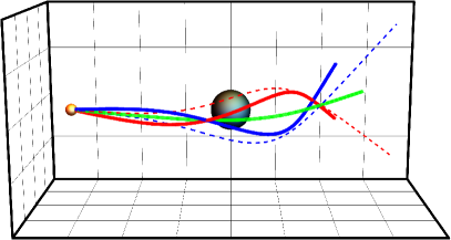
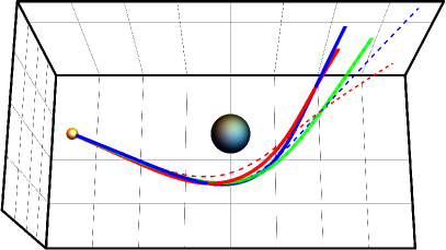
Figure 1: Equatorial view (left) and top view (right) of light rays around a Schwarzschild black hole in Weyl geometry ($C_{2}=C_{3}=\delta=0$). Gravitational spin Hall light rays of opposite circular polarization ($s=\pm 1$, red and blue lines) and a null geodesic ($s=0$, green trajectory) are emitted with the same initial conditions from a source (orange sphere) at $r=8r_{s}$. For comparison, we also display the corresponding gravitational spin Hall rays in Riemann geometry (dashed lines). The individual components of the trajectory and their momenta are shown in Fig. 4.

First, we note that for circularly polarized electromagnetic waves, the WKB field will take the form

$$A_{\alpha}=\sqrt{I}m_{\alpha}e^{i(S+\epsilon\gamma)/\epsilon}\quad\text{or}\quad A_{\alpha}=\sqrt{I}\bar{m}_{\alpha}e^{i(S-\epsilon\gamma)/\epsilon}.$$ (10bm)

The above fields have a total phase factor $\tilde{S}=S+\epsilon s\gamma$, with $s=\pm 1$ depending on the state of circular polarization. While the geometrical optics geodesic ray equations (10aw) were derived by solving a Hamilton-Jacobi equation for the phase function $S$, higher-order corrections and spin-orbit interactions can be taken into account by defining an effective Hamilton-Jacobi equation for the total phase function $\tilde{S}$ [63]. Using the results from the previous section, we can write this as

$$\frac{1}{2}(\tilde{\nabla}_{\mu}\tilde{S})(\tilde{\nabla}^{\mu}\tilde{S})-\epsilon s(\tilde{\nabla}^{\mu}\tilde{S})B_{\mu}=\mathcal{O}(\epsilon^{2}).$$ (10bn)

The polarization-dependent ray equations describing the gravitational spin Hall effect can be derived by applying the method of characteristics to the above equation. In this way we obtain the effective Hamiltonian

$$H(x,p)=\frac{1}{2}g^{\alpha\beta}p_{\alpha}p_{\beta}-\epsilon sp^{\mu}B_{\mu}(x,p)=\mathcal{O}(\epsilon^{2}).$$ (10bo)

The gravitational spin Hall equations can be derived by calculating Hamilton’s equations. However, the above Hamiltonian is gauge dependent, in the sense that the Berry connection depends on the choice of complex vectors $m_{\mu}$ and $\bar{m}_{\mu}$. This gauge dependence can be removed by performing a coordinate transformation of the type introduced in Refs. [77, 49]:

$$x^{\mu} \mapsto x^{\mu}-i\epsilon s\bar{m}^{\nu}\frac{\partial}{\partial p_{\mu}}{m}_{\nu},$$ (10bpa)

$$p_{\mu} \mapsto p_{\mu}+i\epsilon s\left(\bar{m}^{\nu}\tilde{\nabla}_{\mu}{m}_{\nu}+\frac{\alpha}{2}\omega_{\mu}\right).$$ (10bpb)

After performing this coordinate transformation, the Hamiltonian reduces to

$$H(x,p)=\frac{1}{2}g^{\alpha\beta}p_{\alpha}p_{\beta}=\mathcal{O}(\epsilon^{2}),$$ (10bq)

and the gauge-invariant equations of motion describing the gravitational spin Hall effect become

$$\dot{x}^{\mu} =p^{\mu}+\frac{1}{p_{\sigma}t^{\sigma}}S^{\mu\nu}p^{\rho}\tilde{\nabla}_{\rho}t_{\nu},$$ (10bra)

$$\dot{x}^{\nu}\tilde{\nabla}_{\nu}p_{\mu} =-\frac{1}{2}\tilde{R}_{\rho\sigma\mu\nu}p^{\nu}S^{\rho\sigma},$$ (10brb)

In the above equations, $$x^{\mu}(\tau) p_{\mu}(\tau) t^{\mu} S^{\mu\nu}$$ represents the worldline followed by the energy centroid of the electromagnetic wave packet, represents the average momentum of the wave packet, and is a timelike vector field used to define the energy centroid of the wave packet. The spin tensor encodes the state of polarization and the angular momentum carried by the wave packet and is defined as

$$S^{\mu\nu}=2i\epsilon s\bar{m}^{[\mu}m^{\nu]}=\epsilon s\frac{\varepsilon^{\mu\nu\rho\sigma}p_{\rho}t_{\sigma}}{p_{\beta}t^{\beta}}.$$ (10bs)

The gravitational spin Hall equations of motion appear to have the same form as in Riemann geometry. However, the effect of Weyl geometry is hidden in the curvature term from Eq. 10brb, as the symmetry properties of the curvature tensor are not the same in Riemann and Weyl geometry when $\tilde{W}_{\mu\nu}\neq 0$ (see Eq. 10n). Therefore, we must be careful when swapping the indices of the curvature tensor in Eq. 10brb, as terms proportional to $\tilde{W}_{\mu\nu}$ can arise.

A better comparison between the gravitational spin Hall effect in Weyl and Riemann geometry can be achieved by expanding the Weyl covariant derivative and the Weyl curvature tensor in the spin Hall equations. We obtain

$$\dot{x}^{\mu} =p^{\mu}+\frac{1}{p\cdot t}S^{\mu\nu}p^{\rho}\left(\nabla_{\rho}t_{\nu}-\frac{\alpha}{2}t_{\rho}\omega_{\nu}\right),$$ (10bta)

$$\dot{x}^{\nu}\nabla_{\nu}p_{\mu} =-\frac{1}{2}R_{\rho\sigma\mu\nu}p^{\nu}S^{\rho\sigma}$$

$$\qquad-\frac{\alpha}{2p\cdot t}p^{\nu}S^{\rho\sigma}\bigg{(}g_{\mu\sigma}t_{\nu}p^{\gamma}\nabla_{\gamma}\omega_{\rho}$$

$$\qquad-g_{\mu\sigma}\omega_{\nu}p^{\gamma}\nabla_{\gamma}t_{\rho}-g_{\mu\nu}\omega_{\rho}p^{\gamma}\nabla_{\gamma}t_{\sigma}\bigg{)}.$$ (10btb)

In the above form of the spin Hall equations, we can clearly see the effect of the Weyl geometry, given by the terms that contain the Weyl vector field $\omega_{\mu}$.

V Spin Hall effect for Weyl geometric black holes

In this section, we present some numerical examples of gravitational spin Hall trajectories near black holes in Weyl geometry. We consider the family of black hole solutions introduced in Section II.4.

The gravitational spin Hall equations (10br) can be rewritten in a more concrete form by considering the general metric given in Eq. 10ai with $\nu(r)=-\lambda(r)$, a Weyl vector of the form $\omega_{\mu}=(\omega_{0}(r),\omega_{1}(r),0,0)$ and a choice of timelike vector field $t^{\mu}=(e^{-\nu(r)/2},0,0,0)$. We denote the coordinate components of the worldline and the momentum by $x^{\mu}(\tau)=(t(\tau),r(\tau),\theta(\tau),\phi(\tau))$ and $p_{\mu}(\tau)=(p_{t}(\tau),p_{r}(\tau),p_{\theta}(\tau),p_{\phi}(\tau))$, where $\tau$ is an affine parameter. Furthermore, note that we can use the Hamiltonian constraint given in Eq. 10bq to fix one of the components of $p_{\mu}$ and eliminate one of the eight spin Hall equations. Solving Eq. 10bq for $p_{t}$ we obtain

$$p_{t}=-\frac{e^{\frac{\nu}{2}}\sqrt{p_{\phi}^{2}+p_{\theta}^{2}\sin^{2}\theta+e^{\nu}r^{2}p_{r}^{2}\sin^{2}\theta}}{r\sin\theta},$$ (10bu)

where the sign of $p_{t}$ is fixed so that $p^{\mu}$ is future directed. The gravitational spin Hall equations become

$$\dot{t} =-e^{-\nu}p_{t},$$ (10bva)

$$\dot{r} =e^{\nu}p_{r},$$ (10bvb)

$$\dot{\theta} =\frac{p_{\theta}}{r^{2}}+\epsilon s\frac{\alpha\omega_{r}+\nu^{\prime}}{2r^{2}p_{t}\sin\theta}p_{\phi},$$ (10bvc)

$$\dot{\phi} =\frac{p_{\phi}}{r^{2}\sin^{2}\theta}-\epsilon s\frac{\alpha\omega_{r}+\nu^{\prime}}{2r^{2}p_{t}\sin\theta}p_{\theta},$$ (10bvd)

$$\dot{p}_{r} =-\nu^{\prime}e^{\nu}p_{r}^{2}-\frac{\left(r\nu^{\prime}-2\right)\left(p_{\phi}^{2}+p_{\theta}^{2}\sin^{2}\theta\right)}{2r^{3}\sin^{2}\theta},$$ (10bve)

$$\dot{p}_{\theta} =\frac{p_{\phi}^{2}\cot\theta}{r^{2}\sin^{2}\theta}+\epsilon s\frac{e^{\nu}p_{r}\left[\alpha r^{2}\omega_{r}^{\prime}+r\nu^{\prime}\left(\alpha r\omega_{r}+2\right)-2\right]+2p_{r}+p_{\theta}\cot\theta\left(\alpha\omega_{r}+\nu^{\prime}\right)}{2r\sqrt{r^{2}p_{r}^{2}\sin^{2}\theta+e^{-\nu(r)}\left(p_{\phi}^{2}+p_{\theta}^{2}\sin^{2}\theta\right)}}p_{\phi},$$ (10bvf)

$$\dot{p}_{\phi} =\epsilon se^{\nu}\frac{p_{r}p_{\theta}\left[\alpha r^{2}e^{\nu}\omega_{r}^{\prime}+re^{\nu}\left(\alpha r\omega_{r}+2\right)\nu^{\prime}-2e^{\nu}+2\right]+\cot\theta\left(p_{\phi}^{2}\csc^{2}\theta+p_{\theta}^{2}\right)\left(\alpha\omega_{r}+\nu^{\prime}\right)}{2r^{2}p_{t}\csc\theta}.$$ (10bvg)

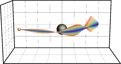
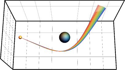
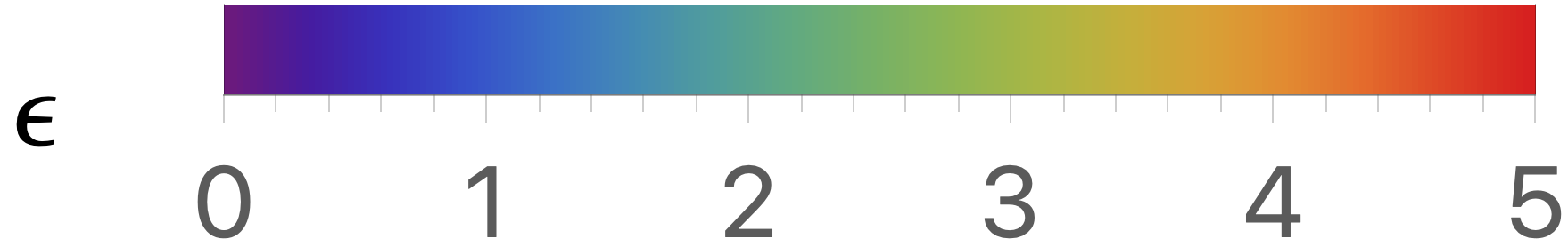
Figure 2: Frequency dependence of the gravitational spin Hall effect of light in Weyl geometry. Equatorial view (left) and top view (right) of light rays of different frequencies (encoded by the colors of the rainbow) and opposite circular polarization, emitted by a source at $r=8r_{s}$ and travelling around a Schwarzschild black hole in Weyl geometry ($C_{2}=C_{3}=\delta=0$).

Note that, in this particular case, the gravitational spin Hall equations do not depend on the time component $\omega_{0}(r)$ of the Weyl vector. We will numerically integrate the above equations using Wolfram Mathematica [78], with a straightforward extension of the code presented in Ref. [79]. For some of the numerical examples presented below, we use unrealistically large values of $\epsilon$ (up to $\epsilon=5$ in units of $M=1$). This is done solely for the purpose of visualization, as otherwise the effect would be very small and would be hardly visible on some of the figures. It should be kept in mind that in physically relevant situations one should only consider $\epsilon<1$, as the WKB expansion used to derive the spin Hall equations is not valid otherwise.

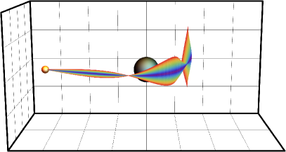
Figure 3: Frequency dependence of the gravitational spin Hall effect of light in Weyl geometry. Equatorial view (left) and top view (right) of light rays of different frequencies (encoded by the colors of the rainbow) and opposite circular polarization, emitted by a source at $r=8r_{s}$ and travelling around a black hole in Weyl geometry with parameters $C_{2}=0$, $C_{3}=5\times 10^{-4}$, $\delta=10^{-2}$.

As a first example, we consider the black hole solution given in Eqs. (10ai) and (10am) with $C_{2}=C_{3}=\delta=0$. In this case, the metric reduces to that of a Schwarzschild black hole. However, even in this case, the Weyl vector will be nonzero. Since this choice of metric represents a black hole solution in both Riemannian and Weyl geometry, it allows us to have a clear comparison between the two and to see how Weyl geometry will affect the propagation of light.

We have shown in the previous Section that null geodesics do not depend on the Weyl vector, and take the same form as in Riemann geometry. However, this is no longer the case for polarized light rays. It can be clearly seen in Eq. (10bt) that the gravitational spin Hall equations have a nontrivial dependence on the Weyl vector (note that Eq. 10bt is independent of the Weyl gauge coupling constant $\alpha$). Thus, in general, we expect that the gravitational spin Hall effect will be different in Weyl and Riemann geometry.

To illustrate this difference, consider the numerical example in Fig. 1. Here, we consider a source of light close to a Schwarzschild black hole, at $r=8r_{s}$, and we emit polarized light rays and geodesics with the same initial conditions. The green trajectory represents a null geodesic, which is the same in both Weyl and Riemann geometry. The red and blue trajectories represent finite-frequency light rays of opposite circular polarization, described by the spin Hall equations. The solid lines represent the gravitational spin Hall rays in Weyl geometry, while the dashed lines represent the gravitational spin Hall trajectories in Riemann geometry. The individual coordinate components of the worldlines, as well as the momenta, are shown in Fig. 4.

Thus, we can clearly see that the gravitational spin Hall effect is different in Weyl and Riemann geometry. In this particular case ($C_{2}=C_{3}=\delta=0$), the polarized light rays experience a stronger deflection toward the Weyl geometry black hole than the corresponding rays in Riemann geometry. This difference gradually fades away as we increase the value of $C_{2}$, and in the limit $C_{2}\rightarrow\infty$ we obtain $\omega_{\mu}\rightarrow 0$ and the gravitational spin Hall rays of Weyl geometry converge to those of Riemann geometry.

Using a similar setup, we also considered the frequency dependence of the gravitational spin Hall effect in Weyl geometry. This is illustrated in Fig. 2, where rays of different frequencies, encoded by the colors of the rainbow, are emitted from a source at $r=8r_{s}$, close to a black hole with $C_{2}=C_{3}=\delta=0$. There are two copies of the rainbow present in Fig. 2, corresponding to the two states of opposite circular polarization ($s=\pm 1$) and separated by a null geodesic trajectory (violet color, corresponding to a wavelength zero).

The individual coordinate components of the worldlines and the momenta are shown in Fig. 5. As expected, light rays with small wavelengths, represented by blue colors, do not deviate too much from the null geodesic trajectory, whereas light rays with large wavelengths, represented by colors close to red, experience a strong deviation.

Another example is shown in Fig. 3, where we considered a more general black hole with $C_{2}=0$, $C_{3}=5\times 10^{-4}$ and $\delta=10^{-2}$. In this case, the general properties of the gravitational spin Hall effect of light remain mostly unchanged, with the exception of the overall magnitude of the deflection, which is now larger and is very sensitive to the values of the parameters $C_{3}$ and $\delta$. The individual coordinate components of the worldlines and the momenta are shown in Fig. 6.

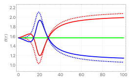
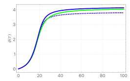
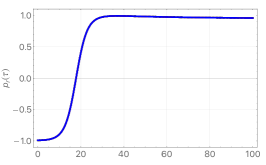
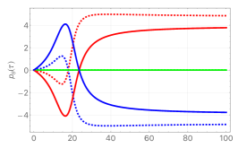
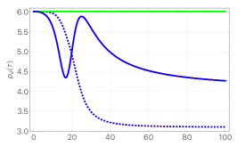
Figure 4: Plots for the individual components of the trajectories $(r(\tau),\theta(\tau),\phi(\tau))$ and the momenta $(p_{r}(\tau),p_{\theta}(\tau),p_{\phi}(\tau))$ for the configuration given in Fig. 1. Green lines represent geodesic motion, solid lines represent spin Hall trajectories of opposite circular polarization in Weyl geometry and dashed lines represent spin Hall trajectories of opposite circular polarization in Riemann geometry. Red or green lines appear to be missing on certain plots because of perfect overlap.

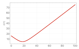
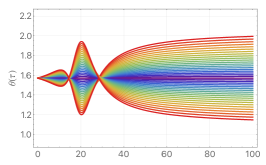
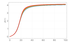
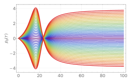
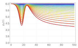
Figure 5: Plots for the individual components of the trajectories $(r(\tau),\theta(\tau),\phi(\tau))$ and the momenta $(p_{r}(\tau),p_{\theta}(\tau),p_{\phi}(\tau))$ for the configuration given in Fig. 2. Different wavelengths $\epsilon$ are encoded in the colors of the rainbow. Lines of certain colors appear to be missing on certain plots because of overlap.

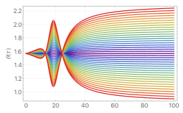
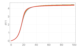
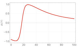
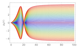
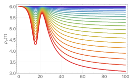
Figure 6: Plots for the individual components of the trajectories $(r(\tau),\theta(\tau),\phi(\tau))$ and the momenta $(p_{r}(\tau),p_{\theta}(\tau),p_{\phi}(\tau))$ for the configuration given in Fig. 3. Different wavelengths $\epsilon$ are encoded in the colors of the rainbow. Lines of certain colors appear to be missing on certain plots because of overlap.

VI Discussions and final remarks

Weyl geometry is an interesting and natural extension of Riemannian geometry. Even though Weyl’s original goal of formulating a successful unified theory of gravitation and electromagnetism was not fulfilled, the purely geometric framework introduced in this geometry has found many applications in physics and even engineering. For example, the mechanics of solids with distributed point defects can be formulated using Weyl geometry, with the geometric object relevant to this distribution being the nonmetricity [80]. The base manifold of a solid with distributed point defects, for a stress-free body, is a flat Weyl manifold, that is, a manifold with an affine connection that has a nonmetricity with vanishing traceless part [80]. Moreover, a large number of metric anomalies (intrinsic interstitials, vacancies, point stacking faults) arising from a distribution of point defects as well as thermal deformations, biological growth, etc. are geometric in nature, and can be analyzed using Weyl geometry [81].

In the present work, we have considered another aspect of Weyl geometry, namely, its effect on the propagation of electromagnetic waves in vacuum, in the presence of a gravitational field. More precisely, we have investigated the frequency-dependent propagation of light, which is the result of the spin-orbit coupling between the external and internal degrees of freedom of electromagnetic waves, and which is described physically with the help of the Berry phase [38, 44, 47]. The spin-orbit coupling leads to the spin Hall effect for light, whose observational detection has opened new perspectives in the study of semiconductor spintronics/valleytronics, in high-energy physics, and in condensed matter physics [82]. It is also important to note that the spin Hall effect for light has a topological nature in the spin-orbit interaction similar to that of the standard spin Hall effect in electronic systems. The theory of the spin Hall effect of light was generalized to the case of Riemannian geometry in [49], where the polarization-dependent ray equations describing the gravitational spin Hall effect of light were obtained. A numerical analysis of the polarization-dependent ray propagation in the Schwarzschild geometry was also presented, and the magnitude of the effect was estimated. It is important to mention that the gravitational spin Hall effect for light is analogous to the spin Hall effect of light in inhomogeneous media, which has been observed experimentally.

A particular and very interesting example of the gravitational spin Hall effect is represented by the deflection of light by a black hole that has the mass of the Sun and a gravitational (Schwarzschild) radius of the order of 3 km, $r_{s}\approx 3$ km. For a circularly polarized light ray coming from a distant source, passing very near the surface of the Sun and then reaching Earth, it turns out that the distance of separation between the rays of opposite circular polarization would depend on the wavelength. For a wavelength of the order $\lambda\approx 10^{-9}$ m, the separation distance of the order $d\approx 10^{-15}$ m. For $\lambda\approx 1$ m, the separation distance is $d\approx 10^{-6}$ m [49]. This ray separation in standard Riemann geometry is very small, $10^{-6}$ times smaller than the wavelength of light. However, it is important to note that the rays are scattered by a finite angle, and after the reintersection point their separation increases linearly with the distance. On the other hand, much more massive compact objects, such as neutron stars or supermassive black holes, could generate a much stronger Riemannian gravitational spin Hall effect of light [49].

It is interesting to point out that the Riemannian gravitational spin Hall equations are just a special case of the Mathisson-Papapetrou equations (see [50] and references therein)

$$\dot{x}^{\mu}\nabla_{\mu}p_{\alpha} =-\frac{1}{2}R_{\alpha\beta\gamma\lambda}\dot{x}^{\beta}S^{\gamma\lambda},$$ (10bwa)

$$\dot{x}^{\mu}\nabla_{\mu}S^{\alpha\beta} =p^{\alpha}\dot{x}^{\beta}-p^{\beta}\dot{x}^{\alpha}.$$ (10bwb)

describing the motion of spinning bodies. To obtain an evolution equation for the worldline, one must impose the Corinaldesi-Papapetrou spin supplementary condition $S^{\alpha\beta}t_{\beta}=0$, where $t_{\beta}$ is a timelike vector field.

The study of the spin Hall effect for light in Weyl geometry is very much simplified by the conformal invariance of Maxwell’s equations. This leads to the important result that in both Riemann and Weyl geometry the electromagnetic field equations take the same form, and thus one can efficiently use again the covariant WKB approximation to study the propagation of light in arbitrary Weyl geometries. However, the polarization-dependent ray equations (10bt) describing the gravitational spin Hall effect of light in Weyl geometry contain the curvature tensor of the Weyl manifold, which introduces a new degree of freedom for the description of the motion, the Weyl vector $\omega_{\mu}$, and its covariant derivatives, respectively.

As an astrophysical application of the general formalism, we have considered the frequency-dependent motion of light in a black hole-type solution of the gravitational field equations in the simplest version of Weyl geometric gravity [34], in which the Weyl vector has only one nonzero component $\omega_{1}$. In this case the Weyl-type field equations do have an exact static spherically symmetric solution, which generalizes the Schwarzschild-de Sitter solutions of general relativity by introducing a new radial distance dependent linear term in the metric. This solution was used in Ref. [35] to propose an alternative geometric description of the galactic rotation curves, and of the galactic properties usually attributed to the existence of dark matter. Within the framework of this model, an effective geometric mass term can be introduced, with an associated density profile. A comparison with a small selected sample of galactic rotation curves was also made by also considering an explicit breaking of the conformal invariance at galactic scales. The parameters of the black hole solution were fixed from the comparison with the observational data as $\gamma=2/C_{2}\approx 10^{-28}$ m^-1, and $C_{1}\approx 10^{4}$. For the integration constant $C_{3}$, it was assumed to have values of the same order of magnitude as the cosmological constant. Hence, the preliminary investigations of [35] indicated that the Weyl geometric theory may represent a viable theoretical explanation for the galactic dynamics without invoking the existence of the mysterious dark matter.

In the exact solution of Weyl geometric gravity $C_{1}$, $C_{2}$ and $C_{3}$ represent integration constants, similar to the gravitational radius (or mass) in the Schwarzschild solution. Hence, their numerical values depend on the considered astrophysical system and may also depend on the mass of the compact object. We have studied numerically the spin Hall effect of light for this Weyl geometric type black hole solution, and investigated the motion of light in this metric, by also performing a detailed comparison with the similar effects in the Schwarzschild geometry. The numerical results indicate a strong effect of Weyl geometry on the polarized light dynamics and a significant increase in its magnitude compared to Riemann geometry. This effect is expected to increase with the distance from the source, and thus astrophysical observations of the spin Hall effect of light, as well as the possible detection of the deviations from the Schwarzschild/Kerr geometries may provide convincing evidence for the presence of the Weyl geometry in the Universe. Therefore, these results on the spin Hall effect of light lead to the possibility of directly constraining the Weyl geometric gravity theory by using astrophysical and astronomical observations of the motion of light emitted near compact objects. In the present work, we have introduced some basic tools necessary for a detailed comparison of the predictions of the spin Hall effect of light in the Weyl geometric gravity theory with the results of astrophysical observations.

Appendix A The curvature tensor in Weyl geometry

In this Appendix, we present the full details of the computation of the curvature tensor in Weyl geometry. Using the decomposition of the Weyl connection given in Eq. 3, we can write

$$\tilde{R}\indices{{}^{\lambda}_{\mu\nu\sigma}} = \partial_{\nu}\Gamma_{\mu\sigma}^{\lambda}-\partial_{\sigma}\Gamma_{\mu\nu}^{\lambda}+\partial_{\nu}\Psi_{\mu\sigma}^{\lambda}-\partial_{\sigma}\Psi_{\mu\nu}^{\lambda}+\left(\Gamma_{\rho\nu}^{\lambda}+\Psi_{\rho\nu}^{\lambda}\right)\left(\Gamma_{\mu\sigma}^{\rho}+\Psi_{\mu\sigma}^{\rho}\right)-\left(\Gamma_{\rho\sigma}^{\lambda}+\Psi_{\rho\sigma}^{\lambda}\right)\left(\Gamma_{\mu\nu}^{\rho}+\Psi_{\mu\nu}^{\rho}\right)$$ (10bx)

$$= R\indices{{}^{\lambda}_{\mu\nu\sigma}}+\partial_{\nu}\Psi_{\mu\sigma}^{\lambda}-\partial_{\sigma}\Psi_{\mu\nu}^{\lambda}+\Gamma_{\rho\nu}^{\lambda}\Psi_{\mu\sigma}^{\rho}+\Gamma_{\mu\sigma}^{\rho}\Psi_{\rho\nu}^{\lambda}-\Gamma_{\rho\sigma}^{\lambda}\Psi_{\mu\nu}^{\rho}-\Gamma_{\mu\nu}^{\rho}\Psi_{\rho\sigma}^{\lambda}+\Psi_{\rho\nu}^{\lambda}\Psi_{\mu\sigma}^{\rho}-\Psi_{\rho\sigma}^{\lambda}\Psi_{\mu\nu}^{\rho}.$$

We have the following relations:

$$\partial_{\nu}\Psi_{\mu\sigma}^{\lambda} =\frac{\alpha}{2}\Big{(}\delta_{\mu}^{\lambda}\partial_{\nu}\omega_{\sigma}+\delta_{\sigma}^{\lambda}\partial_{\nu}\omega_{\mu}-\omega^{\lambda}\partial_{\nu}g_{\mu\sigma}-g_{\mu\sigma}\partial_{\nu}\omega^{\lambda}\Big{)},$$ (10bya)

$$\partial_{\sigma}\Psi_{\mu\nu}^{\lambda} =\frac{\alpha}{2}\Big{(}\delta_{\mu}^{\lambda}\partial_{\sigma}\omega_{\nu}+\delta_{\nu}^{\lambda}\partial_{\sigma}\omega_{\mu}-\omega^{\lambda}\partial_{\sigma}g_{\mu\nu}-g_{\mu\nu}\partial_{\sigma}\omega^{\lambda}\Big{)},$$ (10byb)

Using the above equations, we can write

$$\partial_{\nu}\Psi_{\mu\sigma}^{\lambda}-\partial_{\sigma}\Psi_{\mu\nu}^{\lambda}=\frac{\alpha}{2}\Big{[}\tilde{W}_{\nu\sigma}\delta_{\mu}^{\lambda}+\delta_{\sigma}^{\lambda}\partial_{\nu}\omega_{\mu}-\delta_{\nu}^{\lambda}\partial_{\sigma}\omega_{\mu}-\omega^{\lambda}\left(\partial_{\nu}g_{\mu\sigma}-\partial_{\sigma}g_{\mu\nu}\right)-g_{\mu\sigma}\partial_{\nu}\omega^{\lambda}+g_{\mu\nu}\partial_{\sigma}\omega^{\lambda}\Big{]}.$$ (10bz)

Next, we obtain

$$\Gamma_{\rho\nu}^{\lambda}\Psi_{\mu\sigma}^{\rho} =\frac{\alpha}{2}\left(\Gamma_{\mu\nu}^{\lambda}\omega_{\sigma}+\Gamma_{\sigma\nu}^{\lambda}\omega_{\mu}-\Gamma_{\rho\nu}^{\lambda}g_{\mu\sigma}\omega^{\rho}\right),$$ (10caa)

$$\Gamma_{\mu\sigma}^{\rho}\Psi_{\rho\nu}^{\lambda} =\frac{\alpha}{2}\left(\Gamma_{\mu\sigma}^{\lambda}\omega_{\nu}+\Gamma_{\mu\sigma}^{\rho}\delta_{\nu}^{\lambda}\omega_{\rho}-\Gamma_{\nu\mu\sigma}\omega^{\lambda}\right),$$ (10cab)

$$\Gamma_{\rho\sigma}^{\lambda}\Psi_{\mu\nu}^{\rho} =\frac{\alpha}{2}\left(\Gamma_{\mu\sigma}^{\lambda}\omega_{\nu}+\Gamma_{\nu\sigma}^{\lambda}\omega_{\mu}-\Gamma_{\rho\sigma}^{\lambda}g_{\mu\nu}\omega^{\rho}\right),$$ (10cac)

$$\Gamma_{\mu\nu}^{\rho}\Psi_{\rho\sigma}^{\lambda} =\frac{\alpha}{2}\left(\Gamma_{\mu\nu}^{\lambda}\omega_{\sigma}+\Gamma_{\mu\nu}^{\rho}\delta_{\sigma}^{\lambda}\omega_{\rho}-\Gamma_{\sigma\mu\nu}\omega^{\lambda}\right).$$ (10cad)

Therefore, we find

$$\begin{split}&\Gamma_{\rho\nu}^{\lambda}\Psi_{\mu\sigma}^{\rho}+\Gamma_{\mu\sigma}^{\rho}\Psi_{\rho\nu}^{\lambda}-\Gamma_{\rho\sigma}^{\lambda}\Psi_{\mu\nu}^{\rho}-\Gamma_{\mu\nu}^{\rho}\Psi_{\rho\sigma}^{\lambda}=\frac{\alpha}{2}\Big{(}\Gamma_{\mu\sigma}^{\rho}\delta_{\nu}^{\lambda}\omega_{\rho}-\Gamma_{\mu\nu}^{\rho}\delta_{\sigma}^{\lambda}\omega_{\rho}+\Gamma_{\rho\sigma}^{\lambda}g_{\mu\nu}\omega^{\rho}-\Gamma_{\rho\nu}^{\lambda}g_{\mu\sigma}\omega^{\rho}+\Gamma_{\sigma\mu\nu}\omega^{\lambda}-\Gamma_{\nu\mu\sigma}\omega^{\lambda}\Big{)}.\end{split}$$ (10cb)

Then

$$\partial_{\nu}\Psi_{\mu\sigma}^{\lambda}-\partial_{\sigma}\Gamma_{\mu\nu}^{\lambda}+\Gamma_{\rho\nu}^{\lambda}\Psi_{\mu\sigma}^{\rho}+\Psi_{\rho\nu}^{\lambda}\Gamma_{\mu\sigma}^{\rho}-\Gamma_{\rho\sigma}^{\lambda}\Psi_{\mu\nu}^{\rho}-\Gamma_{\mu\nu}^{\rho}\Psi_{\rho\sigma}^{\lambda}$$ (10cc)

$$= \frac{\alpha}{2}\Bigg{(}\tilde{W}_{\nu\sigma}\delta_{\mu}^{\lambda}+\delta_{\sigma}^{\lambda}\partial_{\nu}\omega_{\mu}-\delta_{\nu}^{\lambda}\partial_{\sigma}\omega_{\mu}-\omega^{\lambda}\partial_{\nu}g_{\mu\sigma}+\omega^{\lambda}\partial_{\sigma}g_{\mu\nu}-g_{\mu\sigma}\partial_{\nu}\omega^{\lambda}+g_{\mu\nu}\partial_{\sigma}\omega^{\lambda}$$

$$-\Gamma_{\rho\nu}^{\lambda}g_{\mu\sigma}\omega^{\rho}+\Gamma_{\rho\sigma}^{\lambda}g_{\mu\nu}\omega^{\rho}+\Gamma_{\mu\sigma}^{\rho}\delta_{\nu}^{\lambda}\omega_{\rho}-\Gamma_{\mu\nu}^{\rho}\delta_{\sigma}^{\lambda}\omega_{\rho}+\Gamma_{\sigma,\mu\nu}\omega^{\lambda}-\Gamma_{\nu,\mu\sigma}\omega^{\lambda}\Bigg{)}.$$

With the use of the relation

$$\Gamma_{\sigma\mu\nu}-\Gamma_{\nu\mu\sigma}=\partial_{\nu}g_{\sigma\mu}-\partial_{\sigma}g_{\mu\nu},$$ (10cd)

we simplify the above equation, thus obtaining

$$\partial_{\nu}\Psi_{\mu\sigma}^{\lambda}-\partial_{\sigma}\Gamma_{\mu\nu}^{\lambda}+\Gamma_{\rho\nu}^{\lambda}\Psi_{\mu\sigma}^{\rho}+\Psi_{\rho\nu}^{\lambda}\Gamma_{\mu\sigma}^{\rho}-\Gamma_{\rho\sigma}^{\lambda}\Psi_{\mu\nu}^{\rho}-\Gamma_{\mu\nu}^{\rho}\Psi_{\rho\sigma}^{\lambda}$$

$$=\frac{\alpha}{2}\Big{(}\tilde{W}_{\nu\sigma}\delta_{\mu}^{\lambda}+\delta_{\sigma}^{\lambda}\nabla_{\nu}\omega_{\mu}-\delta_{\nu}^{\lambda}\nabla_{\sigma}\omega_{\mu}+g_{\mu\nu}\nabla_{\sigma}\omega^{\lambda}-g_{\mu\sigma}\nabla_{\nu}\omega^{\lambda}\Big{)}.$$ (10ce)

The term $\Psi_{\rho\nu}^{\lambda}\Psi_{\mu\sigma}^{\rho}-\Psi_{\rho\sigma}^{\lambda}\Psi_{\mu\nu}^{\rho}$ can be represented in the form

$$\begin{split}\Psi_{\rho\nu}^{\lambda}\Psi_{\mu\sigma}^{\rho}-\Psi_{\rho\sigma}^{\lambda}\Psi_{\mu\nu}^{\rho}=\frac{\alpha^{2}}{4}\Big{[}\left(g_{\mu\nu}\omega_{\rho}\omega^{\rho}-\omega_{\nu}\omega_{\mu}\right)\delta_{\sigma}^{\lambda}-\left(g_{\mu\sigma}\omega_{\rho}\omega^{\rho}-\omega_{\mu}\omega_{\sigma}\right)\delta_{\nu}^{\lambda}+\left(g_{\mu\sigma}\omega_{\nu}-g_{\mu\nu}\omega_{\sigma}\right)\omega^{\lambda}\Big{]}.\end{split}$$ (10cf)

Finally, we obtain the curvature tensor in the Weyl conformal geometry as

$$\tilde{R}\indices{{}^{\lambda}_{\mu\nu\sigma}}=R\indices{{}^{\lambda}_{\mu\nu\sigma}} + \frac{\alpha}{2}\Big{[}\tilde{W}_{\nu\sigma}\delta_{\mu}^{\lambda}+\left(\delta_{\sigma}^{\lambda}\nabla_{\nu}-\delta_{\nu}^{\lambda}\nabla_{\sigma}\right)\omega_{\mu}+\left(g_{\mu\nu}\nabla_{\sigma}-g_{\mu\sigma}\nabla_{\nu}\right)\omega^{\lambda}\Big{]}$$ (10cg)

$$+\frac{\alpha^{2}}{4}\Big{[}\left(\omega^{2}g_{\mu\nu}-\omega_{\mu}\omega_{\nu}\right)\delta_{\sigma}^{\lambda}-\left(\omega^{2}g_{\mu\sigma}-\omega_{\mu}\omega_{\sigma}\right)\delta_{\nu}^{\lambda}+\left(g_{\mu\sigma}\omega_{\nu}-g_{\mu\nu}\omega_{\sigma}\right)\omega^{\lambda}\Big{]},$$

where we used the notation $\omega^{2}=\omega_{\rho}\omega^{\rho}$.

References

- Wald [1984] R. M. Wald, General relativity (University of Chicago Press, Chicago, USA, 1984).
- Côté et al. [2019] J. Côté, V. Faraoni, and A. Giusti, Revisiting the conformal invariance of Maxwell’s equations in curved spacetime, General Relativity and Gravitation 51, 117 (2019).
- Weyl [1918] H. Weyl, Gravitation und Electrizität, Sitzungsberichte der Königlich Preussischen Akademie der Wissenschaften zu Berlin , 465 (1918).
- Scholz [2018] E. Scholz, The Unexpected Resurgence of Weyl Geometry in late 20th-Century Physics, in Beyond Einstein: Perspectives on Geometry, Gravitation, and Cosmology in the Twentieth Century, edited by D. E. Rowe, T. Sauer, and S. A. Walter (Springer New York, New York, NY, 2018) pp. 261–360.
- Penrose [2010] R. Penrose, Cycles of time: an extraordinary new view of the universe (Random House, London, UK, 2010).
- Gurzadyan and Penrose [2013] V. G. Gurzadyan and R. Penrose, On CCC-predicted concentric low-variance circles in the CMB sky, The European Physical Journal Plus 128, 22 (2013).
- Bars et al. [2013] I. Bars, P. J. Steinhardt, and N. Turok, Cyclic cosmology, conformal symmetry and the metastability of the Higgs, Physics Letters B 726, 50 (2013).
- Penrose [2014] R. Penrose, On the Gravitization of Quantum Mechanics 2: Conformal Cyclic Cosmology, Foundations of Physics 44, 873 (2014).
- Tod [2015] P. Tod, The equations of Conformal Cyclic Cosmology, General Relativity and Gravitation 47, 17 (2015).
- ’t Hooft [2015] G. ’t Hooft, Local conformal symmetry: The missing symmetry component for space and time, International Journal of Modern Physics D 24, 1543001 (2015).
- ’t Hooft [2018] G. ’t Hooft, Singularities, horizons, firewalls, and local conformal symmetry, in 2nd Karl Schwarzschild Meeting on Gravitational Physics, edited by P. Nicolini, M. Kaminski, J. Mureika, and M. Bleicher (Springer International Publishing, Cham, 2018) pp. 1–12.
- Karananas and Monin [2016] G. K. Karananas and A. Monin, Weyl vs. conformal, Physics Letters B 757, 257 (2016).
- Dirac [1973] P. A. M. Dirac, Long range forces and broken symmetries, Proceedings of the Royal Society of London. A. Mathematical and Physical Sciences 333, 403 (1973).
- Dirac [1974] P. A. M. Dirac, Cosmological models and the large numbers hypothesis, Proceedings of the Royal Society of London. A. Mathematical and Physical Sciences 338, 439 (1974).
- Rosen [1982] N. Rosen, Weyl’s geometry and physics, Foundations of Physics 12, 213 (1982).
- Israelit [2011] M. Israelit, A Weyl-Dirac cosmological model with DM and DE, General Relativity and Gravitation 43, 751 (2011).
- Utiyama [1973] R. Utiyama, On Weyl’s Gauge Field, Progress of Theoretical Physics 50, 2080 (1973).
- Utiyama [1975a] R. Utiyama, On Weyl’s gauge field, General Relativity and Gravitation 6, 41 (1975a).
- Utiyama [1975b] R. Utiyama, On Weyl’s Gauge Field. II, Progress of Theoretical Physics 53, 565 (1975b).
- Mannheim and Kazanas [1989] P. D. Mannheim and D. Kazanas, Exact Vacuum Solution to Conformal Weyl Gravity and Galactic Rotation Curves, The Astrophysical Journal 342, 635 (1989).
- Mannheim [1994] P. D. Mannheim, Open questions in classical gravity, Foundations of Physics 24, 487 (1994).
- Mannheim [1996] P. D. Mannheim, Local and global gravity, Foundations of Physics 26, 1683 (1996).
- Mannheim [2000] P. D. Mannheim, Attractive and repulsive gravity, Foundations of Physics 30, 709 (2000).
- Mannheim [2007] P. D. Mannheim, Solution to the ghost problem in fourth order derivative theories, Foundations of Physics 37, 532 (2007).
- Mannheim [2012] P. D. Mannheim, Making the case for conformal gravity, Foundations of Physics 42, 388 (2012).
- Ghilencea [2019a] D. M. Ghilencea, Spontaneous breaking of Weyl quadratic gravity to Einstein action and Higgs potential, Journal of High Energy Physics 2019, 49 (2019a).
- Ghilencea and Lee [2019] D. M. Ghilencea and H. M. Lee, Weyl gauge symmetry and its spontaneous breaking in the standard model and inflation, Physical Review D 99, 115007 (2019).
- Ghilencea [2019b] D. M. Ghilencea, Weyl inflation with an emergent Planck scale, Journal of High Energy Physics 2019, 209 (2019b).
- Ghilencea [2020a] D. M. Ghilencea, Stueckelberg breaking of Weyl conformal geometry and applications to gravity, Physical Review D 101, 045010 (2020a).
- Ghilencea [2020b] D. M. Ghilencea, Palatini quadratic gravity: spontaneous breaking of gauged scale symmetry and inflation, The European Physical Journal C 80, 1147 (2020b).
- Ghilencea [2021] D. M. Ghilencea, Gauging scale symmetry and inflation: Weyl versus Palatini gravity, The European Physical Journal C 81, 510 (2021).
- Ghilencea [2022] D. M. Ghilencea, Standard Model in Weyl conformal geometry, The European Physical Journal C 82, 23 (2022).
- Ghilencea [2023] D. M. Ghilencea, Non-metric geometry as the origin of mass in gauge theories of scale invariance, The European Physical Journal C 83, 176 (2023).
- Yang et al. [2022] J.-Z. Yang, S. Shahidi, and T. Harko, Black hole solutions in the quadratic Weyl conformal geometric theory of gravity, The European Physical Journal C 82, 1171 (2022).
- Burikham et al. [2023] P. Burikham, T. Harko, K. Pimsamarn, and S. Shahidi, Dark matter as a Weyl geometric effect, Physical Review D 107, 064008 (2023).
- Sinova et al. [2015] J. Sinova, S. O. Valenzuela, J. Wunderlich, C. H. Back, and T. Jungwirth, Spin Hall effects, Reviews of Modern Physics 87, 1213 (2015).
- Dyakonov and Khaetskii [2008] M. I. Dyakonov and A. V. Khaetskii, Spin Hall Effect, in Spin Physics in Semiconductors, edited by M. I. Dyakonov (Springer Berlin Heidelberg, 2008) pp. 211–243.
- Bliokh et al. [2015a] K. Y. Bliokh, F. J. Rodríguez-Fortuño, F. Nori, and A. V. Zayats, Spin-orbit interactions of light, Nature Photonics 9, 796 (2015a).
- Kim et al. [2023] M. Kim, Y. Yang, D. Lee, Y. Kim, H. Kim, and J. Rho, Spin Hall Effect of Light: From Fundamentals To Recent Advancements, Laser & Photonics Reviews 17, 2200046 (2023).
- Dyakonov and Perel [1971a] M. I. Dyakonov and V. I. Perel, Possibility of orienting electron spins with current, Soviet Journal of Experimental and Theoretical Physics Letters 13, 467 (1971a).
- Dyakonov and Perel [1971b] M. I. Dyakonov and V. I. Perel, Current-induced spin orientation of electrons in semiconductors, Physics Letters A 35, 459 (1971b).
- Bakun et al. [1984] A. A. Bakun, B. P. Zakharchenya, A. A. Rogachev, M. N. Tkachuk, and V. G. Fleǐsher, Observation of a surface photocurrent caused by optical orientation of electrons in a semiconductor, Soviet Journal of Experimental and Theoretical Physics Letters 40, 1293 (1984).
- Kato et al. [2004] Y. K. Kato, R. C. Myers, A. C. Gossard, and D. D. Awschalom, Observation of the spin Hall effect in semiconductors, Science 306, 1910 (2004).
- Bliokh et al. [2015b] K. Y. Bliokh, D. Smirnova, and F. Nori, Quantum spin Hall effect of light, Science 348, 1448 (2015b).
- Hosten and Kwiat [2008] O. Hosten and P. Kwiat, Observation of the spin Hall effect of light via weak measurements, Science 319, 787 (2008).
- Bliokh et al. [2008a] K. Y. Bliokh, A. Niv, V. Kleiner, and E. Hasman, Geometrodynamics of spinning light, Nature Photonics 2, 748 (2008a).
- Bliokh and Bliokh [2006] K. Y. Bliokh and Y. P. Bliokh, Conservation of Angular Momentum, Transverse Shift, and Spin Hall Effect in Reflection and Refraction of an Electromagnetic Wave Packet, Physical Review Letters 96, 073903 (2006).
- Onoda et al. [2004] M. Onoda, S. Murakami, and N. Nagaosa, Hall effect of light, Physical Review Letters 93, 083901 (2004).
- Oancea et al. [2020] M. A. Oancea, J. Joudioux, I. Y. Dodin, D. E. Ruiz, C. F. Paganini, and L. Andersson, Gravitational spin Hall effect of light, Physical Review D 102, 024075 (2020).
- Harte and Oancea [2022] A. I. Harte and M. A. Oancea, Spin Hall effects and the localization of massless spinning particles, Physical Review D 105, 104061 (2022).
- Gosselin et al. [2007] P. Gosselin, A. Bérard, and H. Mohrbach, Spin Hall effect of photons in a static gravitational field, Physical Review D 75, 084035 (2007).
- Frolov [2020] V. P. Frolov, Maxwell equations in a curved spacetime: Spin optics approximation, Physical Review D 102, 084013 (2020).
- Andersson et al. [2021] L. Andersson, J. Joudioux, M. A. Oancea, and A. Raj, Propagation of polarized gravitational waves, Physical Review D 103, 044053 (2021).
- Oancea et al. [2022] M. A. Oancea, R. Stiskalek, and M. Zumalacárregui, From the gates of the abyss: Frequency- and polarization-dependent lensing of gravitational waves in strong gravitational fields, arXiv:2209.06459 (2022).
- Yamamoto [2018] N. Yamamoto, Spin Hall effect of gravitational waves, Physical Review D 98, 061701 (2018).
- Audretsch [1981] J. Audretsch, Trajectories and spin motion of massive spin- particles in gravitational fields, Journal of Physics A: Mathematical and General 14, 411 (1981).
- Rüdiger [1981] R. Rüdiger, The Dirac equation and spinning particles in general relativity, Proceedings of the Royal Society A: Mathematical, Physical and Engineering Sciences 377, 417 (1981).
- Oancea and Kumar [2023] M. A. Oancea and A. Kumar, Semiclassical analysis of dirac fields on curved spacetime, Physical Review D 107, 044029 (2023).
- Marsot et al. [2022a] L. Marsot, P.-M. Zhang, and P. A. Horvathy, Anyonic spin-Hall effect on the black hole horizon, Physical Review D 106, L121503 (2022a).
- Gray et al. [2022] F. Gray, D. Kubizňák, T. R. Perche, and J. Redondo-Yuste, Carrollian Motion in Magnetized Black Hole Horizons, arXiv:2211.13695 (2022).
- Marsot et al. [2022b] L. Marsot, P.-M. Zhang, M. Chernodub, and P. Horvathy, Hall effects in Carroll dynamics, arXiv:2212.02360 (2022b).
- Bičák et al. [2022] J. Bičák, D. Kubizňák, and T. R. Peche, Monarch Migration of Carrollian Particles on the Black Hole Horizon, arXiv:2302.11639 (2022).
- Andersson and Oancea [2023] L. Andersson and M. A. Oancea, Spin Hall effects in the sky, arXiv:2302.13634 (2023).
- Oancea et al. [2019] M. A. Oancea, C. F. Paganini, J. Joudioux, and L. Andersson, An overview of the gravitational spin Hall effect, arXiv:1904.09963 (2019).
- Panpanich and Burikham [2018] S. Panpanich and P. Burikham, Fitting rotation curves of galaxies by de Rham-Gabadadze-Tolley massive gravity, Physical Review D 98, 064008 (2018).
- Bliokh et al. [2008b] K. Y. Bliokh, Y. Gorodetski, V. Kleiner, and E. Hasman, Coriolis Effect in Optics: Unified Geometric Phase and Spin-Hall Effect, Physical Review Letters 101, 030404 (2008b).
- Bliokh [2009] K. Y. Bliokh, Geometrodynamics of polarized light: Berry phase and spin Hall effect in a gradient-index medium, Journal of Optics A: Pure and Applied Optics 11, 094009 (2009).
- Duval et al. [2006] C. Duval, Z. Horváth, and P. A. Horváthy, Fermat principle for spinning light, Physical Review D 74, 021701 (2006).
- Duval et al. [2007] C. Duval, Z. Horváth, and P. A. Horváthy, Geometrical spinoptics and the optical Hall effect, Journal of Geometry and Physics 57, 925 (2007).
- Ruiz and Dodin [2015] D. E. Ruiz and I. Y. Dodin, First-principles variational formulation of polarization effects in geometrical optics, Physical Review A 92, 043805 (2015).
- Eddington [1920] A. S. Eddington, Space, time and gravitation: An outline of the general relativity theory (University Press, 1920).
- Gordon [1923] W. Gordon, Zur lichtfortpflanzung nach der relativitätstheorie, Annalen der Physik 377, 421 (1923).
- Skrotskii [1957] G. V. Skrotskii, The Influence of Gravitation on the Propagation of Light, Soviet Physics Doklady 2, 226 (1957).
- Plebanski [1960] J. Plebanski, Electromagnetic waves in gravitational fields, Physical Review 118, 1396 (1960).
- de Felice [1971] F. de Felice, On the gravitational field acting as an optical medium, General Relativity and Gravitation 2, 347 (1971).
- Fathi and Thompson [2016] M. Fathi and R. T. Thompson, Cartographic distortions make dielectric spacetime analog models imperfect mimickers, Physical Review D 93, 124026 (2016).
- Littlejohn and Flynn [1991] R. G. Littlejohn and W. G. Flynn, Geometric phases in the asymptotic theory of coupled wave equations, Physical Review A 44, 5239 (1991).
- Wolfram Research, Inc. [2021] Wolfram Research, Inc., Mathematica, Version 13.0.0 (2021), Champaign, IL, 2021.
- Oancea [2021] M. A. Oancea, Spin Hall effects in General Relativity, University of Potsdam , PhD thesis (2021).
- Yavari and Goriely [2012] A. Yavari and A. Goriely, Weyl geometry and the nonlinear mechanics of distributed point defects, Proceedings of the Royal Society A: Mathematical, Physical and Engineering Sciences 468, 3902 (2012).
- Roychowdhury and Gupta [2017] A. Roychowdhury and A. Gupta, Non-metric connection and metric anomalies in materially uniform elastic solids, Journal of Elasticity 126, 1 (2017).
- Ling et al. [2017] X. Ling, X. Zhou, K. Huang, Y. Liu, C.-W. Qiu, H. Luo, and S. Wen, Recent advances in the spin Hall effect of light, Reports on Progress in Physics 80, 066401 (2017).