Taylor-Couette flow in an elliptical enclosure generated by an inner rotating circular cylinder

Abstract

Taylor-Couette flow between rotating cylinders is a classical problem in fluid mechanics and has been extensively studied in the case of two concentric circular cylinders. There have been relatively small number of studies in complex-shaped cylinders with one or both cylinders rotating. In this paper, we study the characteristics of Taylor cells in an elliptical outer cylinder with a rotating concentric inner circular cylinder. We numerically solve the three-dimensional unsteady Navier-Stokes equations assuming periodicity in the axial direction. We use a Fourier-spectral meshless discretization by interpolating variables at scattered points using polyharmonic splines and appended polynomials. A pressure-projection algorithm is used to advance the flow equations in time. Results are presented for an ellipse of aspect ratio two and for several flow Reynolds numbers ($Re=\omega r_{i}(b-r_{i}))/\nu$, where $\omega$ = angular velocity [rad/s], $r_{i}$ = radius of inner cylinder, $b$ = semi-minor axis, and $\nu$ = kinematic viscosity) from subcritical to 300. Streamlines, contours of axial velocity, pressure, vorticity, and temperature are presented along with surfaces of Q criterion. The flow is observed to be steady until $Re=300$ and unsteady at $Re=350$.

1 Introduction

The Taylor-Couette flow [1, 2, 3, 4] between two rotating concentric circular cylinders has been extensively studied in literature since the early works of Mallock [1, 2], Couette [3], and Taylor [4]. Numerous experimental and computational studies have been since conducted at Reynolds numbers that range from subcritical to supercritical regimes, and to the turbulent regime. It has been well documented that at modest Reynolds numbers, the initially two-dimensional flow between the concentric circular cylinders bifurcates to a three-dimensional flow with pairs of toroidal vortices known as Taylor cells. As the Reynolds number is increased, the steady Taylor cells transition to spiral vortices, unsteady chaotic flow, and eventually to turbulence [5, 6, 7, 8, 9]. The widely studied geometry has been the two-dimensional concentric cylinders configuration with narrow and wide gaps [10, 11, 12, 13, 14, 15, 16] in tall as well as short aspect ratio geometries [17, 18, 19, 20]. Numerical simulations [21, 22, 23, 24, 25] and Particle Image Velocimetry studies [26, 27] have provided detailed structure and transitions of these cells. A collage of fascinating flow patterns from steady toroidal vortices to travelling waves, spiral wavy vortices, and mixed laminar/turbulent patches have been observed. Coles [5] reported several different flow patterns for gap Reynolds number between 114 and 1600 including patches of laminar and turbulent regions in an alternating spiral pattern. Andereck et al. [6] conducted experiments with varying combinations of both inner and outer cylinders rotating and observed that the number of azimuthal wave modes increases for a counter-rotating outer cylinder compared to a stationary outer cylinder. By increasing the rotational speeds of the inner and outer cylinders, many flow regimes ranging from modulated wavy vortices to intermittent and spiral turbulence, and a featureless turbulent flow at Re of 1000 were observed. Numerous practical applications of the Taylor-Couette flow have been developed for particle separation [28, 29, 30, 31], membrane filtration [32, 28, 33, 34, 35], desalination [36], and devices for chemical reaction engineering [37]. For continuous operation of separation devices, the extended Taylor-Couette-Poiseuille flow [38, 39, 40] has been studied extensively. Studies of heat transfer in Taylor-Couette flow have also been conducted with constant temperature and constant heat flux boundary conditions [41, 42, 43, 44, 45].

While the most widely studied configuration has been the concentric cylinder geometry, geometrical variations in the shapes of the cylinders provide a large and uncharted opportunity for exploring the rich fluid physics and exploiting them for new device development. Geometrical variations to the coaxial configuration may include change of the cross-sectional shapes of the inner and outer cylinders (with uniformity in the axial direction), axial changes to the cross-sectional dimensions, and creation of periodic disturbances to name a few. The widely studied cross-sectional shape is an eccentrically placed inner circular cylinder which produces a non-axisymmetric base flow whose stability characteristics are different from the concentric case. Such a configuration not only alters the base sub-critical flow but also the super-critical states of the Taylor cells [46, 47, 48, 49]. Krueger et al. [49] performed experiments to determine the critical rotation rates for different values of eccentricity. As the eccentricity is increased, it is found that the flow became more unstable, forming Taylor cells at earlier Reynolds numbers. A linear stability analysis performed by Oikawa et al. [47] indicates that the subcritical flow becomes unstable at lower Reynolds numbers as the eccentricity is increased. Rui-Xiu et al. [50] used the approach of Stuart and Di Prima [14], DiPrima and Stuart [10, 11, 12], DiPrima and Eagles [13] to investigate the linear stability of flow between the eccentric cylinders and found results in agreement with previous studies. Stability of eccentric Taylor-Couette-Poiseuille flow was studied by Leclercq et al. [51, 52] using a bipolar coordinate system.

In contrast to the amount of research conducted on the basic Taylor-Couette geometry, there have been only a small number of studies of Taylor cells in other configurations. Sprague et al. [53], Sprague and Weidman [54] considered a geometry in which the Taylor vortices are continuously tailored by changing both the inner and outer cylinder radii. In concentric spheres, with the inner sphere rotating, Wimmer [55], Nakabayashi and Tsuchida [56, 57] showed the occurrence of Taylor vortices. Subsequently Wimmer [58] extended the study to ellipsoids and coaxial cones. Denne and Wimmer [59] observed that the Taylor vortices in coaxial cones have a different structure than the cylindrical Taylor-Couette flow. Soos et al. [60] simulated the flow development in a mixer with a rotating lobed inner cylinder inside a circular outer cylinder. They observed enhanced mixing in three- and four-lobed configurations resulting from the cyclic squeezing and expansion of the Taylor cells. Snyder [61, 8, 9] considered a square outer cylinder with a smooth inner circular cylinder and experimentally characterized the Taylor cells. A similar experiment with short cylinders was performed by Mullin and Lorenzen [62] who found anomalous modes when the end wall boundary layers interacted with the Taylor cells. Such anomalous cells were also observed by Benjamin and Mullin [63], and Lorenzen and Mullin [17] at higher Reynolds numbers. One configuration where the inner rotating cylinder is ribbed was considered by Greidanus et al. [64]. They measured the drag and torque on the rotating cylinder and found a reduction of $5.3\%$ in drag at a turbulent Reynolds number of $4.7\times 10^{4}$. The ribs were placed vertically along the circumference of the inner cylinder. The riblets were of small dimension and did not alter the macroscopic features of the main Taylor vortices but contributed to reduction in the drag by the turbulent boundary layer. Razzak et al. [65] considered axial bellows where the outer cylinders contained waves of a certain amplitude and wavelength. The numerical study characterized the flow patterns, distributions of velocities and pressure within the bellow cavities at different Reynolds numbers. Recently, Kumar [66] studied a geometry with the outer wall diffusing at a fixed angle. The three-dimensional flow fields were computed for different diffuser angles and different Reynolds numbers. The structure of the Taylor cells was documented in both steady and unsteady regimes. Other geometries where the cross-section varies in the axial direction are cones and spheres [55, 58, 59, 56, 57]. A stability analysis of flow between an outer non-circular cylinder and a coaxial inner cylinder was reported by Eagles and Soundalgekar [67]. Another non-traditional geometry in which Taylor vortices have been investigated is a “stadium” where two semi-circular end chambers are connected to a rectangular enclosure [68].

The present paper deals with a novel geometry in which we have not found any studies of the structure and characteristics of Taylor vortices. The geometry is an elliptical cylinder inside which a circular cylinder is placed concentrically. The inner cylinder is rotated while the outer one is stationary. Such a geometry has applications to lubrication inside elliptical bearings [69, 70, 71, 72, 73]. The base flow in an elliptical cylinder with a rotating inner cylinder is more complex than that in an eccentric circular cylinder configuration because of the formation of corner vortices. Because of the larger gap along the major axis of the ellipse, the circular motion created by the inner rotating cylinder drives another set of counter-rotating vortices akin to the Moffatt vortices in shear driven cavities [74, 75, 76, 77, 78, 79, 80, 81]. The two-dimensional flow inside an ellipse with a rotating cylinder was recently investigated by us [82] using a high accuracy meshless solution procedure [83, 84, 85, 86]. In [82], we reported the effects of Reynolds number, aspect ratio of ellipse, and the eccentricity of placement of the inner cylinder on the flow and pressure fields. The numerical algorithm and the flow were two-dimensional and did not capture any three-dimensional vortices generated by instabilities of the base flow.

In this paper, we present results of a three-dimensional study performed with a recently developed Fourier spectral meshless method. The Fourier spectral method assumes periodicity in the axial direction and solves the Navier-Stokes equations in Fourier space at scattered locations in the cross-stream plane. We show the formation of Taylor vortices similar to those in circular cylinders with differences arising due to the squeezing and expansion of the vortices as the flow passes through the major and minor axes. Section 2 first briefly describes the numerical algorithm. Section 3 presents results of validation and grid-independency tests. Results for concentric placement of the inner cylinder are given in Section 4. A summary of major findings is given in Section 5.

2 Methodology

2.1 Flow Geometry and Equations Solved

The flow geometry studied is shown in Figure 1. An inner cylinder of radius $r_{i}$ rotates inside an ellipse of the semi major axis $a$ and semi minor axis $b$. In this study, the aspect ratio $a/b$ is taken as two, and the gap $(b-r_{i})$ is taken to be equal to $r_{i}$. Thus, the semi minor axis of the ellipse is twice the inner cylinder radius. Non-dimensionally, we have taken the radius of the inner cylinder to be $0.5$, and the gap to be $0.5$. The flow is considered periodic in the axial ($z$) direction, and the number of wave numbers resolved in Fourier space is decided based on the energy decay with wave number. The flow Reynolds number is defined as $Re=\omega r_{i}(b-r_{i})/\nu$, where $\omega$ is the speed of rotation (rad/s) of the inner cylinder and $\nu$ is the fluid kinematic viscosity. The fluid is considered Newtonian, and the density and viscosity are considered constant. The flow is considered to be incompressible.

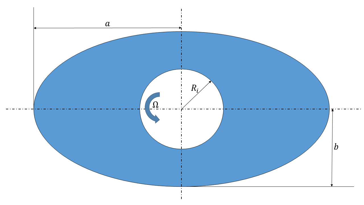
Figure 1: The cross section of the model analysed in this study

The walls of the cylinders are taken as non-penetrating and have no slip. For the heat transfer computations, the inner wall is heated at a non-dimensional temperature of one, and the outer wall is held at a non-dimensional temperature of zero. The three-dimensional time-dependent equations are solved marching in time to determine the onset of unsteadiness of the flow with the Reynolds number. The equations solved are

$$\frac{\partial u_{i}}{\partial x_{i}} =0;$$ (1)

$$\rho\left(\frac{\partial u_{i}}{\partial t}+u_{j}\frac{\partial u_{i}}{\partial x_{j}}\right) =-\frac{\partial p}{\partial x_{i}}+\mu\nabla^{2}u_{i}$$ (2)

$$\rho c_{p}\left(\frac{\partial T}{\partial t}+u_{j}\frac{\partial T}{\partial x_{j}}\right) =k\nabla^{2}T+S$$ (3)

where, $\mu$ is dynamic viscosity of fluid, $\rho$ is the density of the fluid, $T$ is the temperature, $u_{i}$ are components of velocity, $k$ is the thermal conductivity and $S$ denotes the source term. Here the tensor summation notation is used for the continuity equation and the advection terms. The steady state is assumed when the differences in values at adjacent time steps have decreased below $10^{-5}$ non-dimensional units. The torque and Nusselt number are also computed in time and compared between time steps. The non-dimensional torque is computed as

$$\tau_{c}=\mu r_{i}u_{\theta}L$$ (4)

where, $u_{\theta}$ is the tangential velocity of the inner cylinder, $r_{i}$ is the radius of inner cylinder and $L$ is the length in the axial direction. The Nusselt number is computed using the relation

$$Nu=\frac{2r_{i}}{k_{t}}\left(\frac{1}{2\pi r_{i}L\Delta T}\int_{\theta=0}^{\theta=2\pi}\int_{z=0}^{z=L}\left[k_{t}\frac{\partial T}{\partial r}r_{i}\right]d\theta dz\right)$$ (5)

where $k_{t}$ is the thermal conductivity, and $\Delta T$ is the temperature difference between the inner and outer cylinders.

2.2 Numerical Method

2.2.1 Spectral Decomposition

To implement the third dimention of the Cartesian space, a Fourier spectral method is used. Because of periodicity, the governing variables, $\psi(x,y,z,t)$, are first expressed in Fourier space by the expansion (Fornberg [87], Canuto et al. [88]):

$$\psi\left(x,y,z_{l},t\right)=\sum_{k=-N}^{k=N}\widehat{\psi_{k}}(x,y,t)\exp\left(\mathrm{i}kz_{l}\right),\quad l=0,1,...,2N$$ (6)

where, $\widehat{\psi_{k}}$ is a complex valued function corresponding to wave number $k$ ranging from $-N$ to $N$ and $\mathfrak{i}^{2}=-1$. $\widehat{\psi_{k}}$ can be represented with an inverse Fourier transform given as in eq. 7. $\psi$ being a real valued function (the field variables), the transform coefficient functions $\widehat{\psi_{k}}(x,y,t)$ are complex conjugates for positive and negative values of $k$.

$$\widehat{\psi_{k}}(x,y,t)=\frac{1}{2N+1}\sum_{l=0}^{l=2N}\psi\left(x,y,z_{l},t\right)\exp\left(-\mathfrak{i}kz_{l}\right),\quad k=-N,...,0,...,N$$ (7)

The partial differential equations can be transformed to wave number space by computing each derivative in the transformed space. For example, the partial differential equation

$$\frac{\partial\psi}{\partial t}+\left[\frac{\partial(u\psi)}{\partial x}+\frac{\partial(v\psi)}{\partial y}+\frac{\partial(w\psi)}{\partial z}\right]=\Gamma\left[\frac{\partial^{2}\psi}{\partial x^{2}}+\frac{\partial^{2}\psi}{\partial y^{2}}+\frac{\partial^{2}\psi}{\partial z^{2}}\right]+S$$ (8)

in transformed space becomes

$$\frac{\partial\widehat{\psi_{k}}}{\partial t}+\left[\frac{\partial\widehat{(u\psi)_{k}}}{\partial x}+\frac{\partial\widehat{(v\psi)_{k}}}{\partial y}+\mathfrak{i}\widehat{k(w\psi)_{k}}\right]=\Gamma\left[\frac{\partial^{2}\widehat{\psi_{k}}}{\partial x^{2}}+\frac{\partial^{2}\widehat{\psi_{k}}}{\partial y^{2}}-k^{2}\widehat{\psi_{k}}\right]+\widehat{S_{k}}$$ (9)

where, $[u,v,w]$ are components of velocity, $\Gamma$ is diffusion coefficient and $S$ is the source term.

For integrating the time-dependent Navier-Stokes equations, we use the popular fractional step procedure [89] which consists of a momentum step, followed by a pressure computation step which projects the momentum velocities to a divergence-free state. In our current work, we use an explicit procedure to compute advection and diffusion fluxes. However, the pressure-projection step requires solution of an implicit equation, and thus an iterative algorithm. The momentum step computes intermediate values for the velocities by explicitly updating them in wave number space. Thus,

$$\frac{\widehat{\tilde{u}_{k}}-\widehat{u_{k}^{n}}}{\Delta t} =-\left[\frac{\partial\widehat{(\left.u^{n}u^{n}\right)_{k}}}{\partial x}+\frac{\partial\widehat{(\left.v^{n}u^{n}\right)_{k}}}{\partial y}+\mathfrak{i}k\widehat{(\left.w^{n}u^{n}\right)_{k}}\right]+\nu\left[\frac{\partial^{2}\widehat{u_{k}^{n}}}{\partial x^{2}}+\frac{\partial^{2}\widehat{u_{k}^{n}}}{\partial y^{2}}-k^{2}\widehat{u_{k}^{n}}\right]$$ (10)

$$\frac{\widehat{\tilde{v}_{k}}-\widehat{v_{k}^{n}}}{\Delta t} =-\left[\frac{\partial\widehat{(\left.u^{n}v^{n}\right)_{k}}}{\partial x}+\frac{\partial\widehat{(\left.v^{n}v^{n}\right)_{k}}}{\partial y}+\mathfrak{i}k\widehat{(\left.w^{n}v^{n}\right)_{k}}\right]+\nu\left[\frac{\partial^{2}\widehat{v_{k}^{n}}}{\partial x^{2}}+\frac{\partial^{2}\widehat{v_{k}^{n}}}{\partial y^{2}}-k^{2}\widehat{v_{k}^{n}}\right]$$ (11)

$$\frac{\widehat{\tilde{w}_{k}}-\widehat{w_{k}^{n}}}{\Delta t} =-\left[\frac{\partial\widehat{(\left.u^{n}w^{n}\right)_{k}}}{\partial x}+\frac{\partial\widehat{(\left.v^{n}w^{n}\right)_{k}}}{\partial y}+\mathfrak{i}k\widehat{(\left.w^{n}w^{n}\right)_{k}}\right]+\nu\left[\frac{\partial^{2}\widehat{w_{k}^{n}}}{\partial x^{2}}+\frac{\partial^{2}\widehat{w_{k}^{n}}}{\partial y^{2}}-k^{2}\widehat{w_{k}^{n}}\right]$$ (12)

The superscript $n$ denotes values at previous time step. Note that the explicit time step is usually much more restrictive than that of a semi-implicit or fully implicit algorithm. However, the explicit algorithm is simpler to implement. Since these momentum velocities do not satisfy the continuity equation, a pressure Poisson equation is solved to project the intermediate velocities to a divergence-free state. The pressure Poisson equation in wave space is given by

$$\frac{\partial^{2}\widehat{p_{k}^{n+1}}}{\partial x^{2}}+\frac{\partial^{2}\widehat{p_{k}^{n+1}}}{\partial y^{2}}-k^{2}\widehat{p_{k}^{n+1}}=\frac{\rho}{\Delta t}\left[\frac{\partial\widehat{\tilde{u}_{k}}}{\partial x}+\frac{\partial\widehat{\tilde{v}_{k}}}{\partial y}+\mathrm{i}k\widehat{\tilde{w}_{k}}\right]$$ (13)

After the pressure Poisson equation is solved, the momentum velocities are corrected in wave space as

$$\widehat{u_{k}^{n+1}}=\widehat{\tilde{u_{k}}}-\frac{\Delta t}{\rho}\frac{\partial\widehat{p_{k}^{n+1}}}{\partial x}$$ (14)

$$\widehat{v_{k}^{n+1}}=\widehat{\tilde{v}_{k}}-\frac{\Delta t}{\rho}\frac{\partial\widehat{p_{k}^{n+1}}}{\partial y}$$

$$\widehat{w_{k}^{n+1}}=\widehat{\tilde{w}_{k}}-\frac{\Delta t}{\rho}\mathrm{i}k\widehat{p_{k}^{n+1}}$$

Once the velocities are updated in wave space, they are back-transformed to physical space for computation of the next time step values. The temperature equation is subsequently solved with explicit computation of the advection and diffusion terms. To compute the cross-stream derivatives $\frac{\partial\psi}{\partial x}$,$\frac{\partial\psi}{\partial y}$, etc. we use a meshless method that interpolates variables at scattered data using polyharmonic radial basis functions (PHS-RBF). For complex geometries, it is common to use unstructured finite volume methods [90] or finite element methods. Here we use the meshless method for the flexibility and accuracy it provides. We discretize the cross-section by a set of scattered points generated here as vertices of a finite element grid, using the GMSH software [91]. The set of scattered points do not use any underlying grid and are not connected by edges and elements.

The first step in the meshless method is to interpolate a variable between the scattered points. We use a cloud based interpolation in which any variable at a base point is interpolated over a cloud of neighbor points using the PHS-RBF. An arbitrary variable $s(\textbf{x})$ is interpolated as

$$s(\textbf{x})=\sum_{i=1}^{q}\lambda_{i}\phi(||\bm{x}-\bm{x_{i}}||_{2})+\sum_{i=1}^{m}\gamma_{i}P_{i}(\bm{x})$$ (15)

where, $\phi(r)=r^{2a_{1}+1},\hskip 2.84544pta_{1}\in\mathbb{N}$ is the PHS-RBF, $m$ is the number of monomials ($P_{i}$) upto a maximum degree of $l$ and $(\lambda_{i},\gamma_{i})$ are $q+m$ coefficients. We use $a_{1}=1$ in this study. $q$ equations are obtained by collocating eq. 15 over the $q$ cloud points. $m$ additional equations required to close the linear system are imposed as constraints on the polynomials [92]:

$$\sum_{i=1}^{q}\lambda_{i}P_{j}(\bm{x_{i}})=0\hskip 14.22636pt\text{for }1\leq j\leq m$$ (16)

In a matrix vector form, we can write these equations as

$$\begin{bmatrix}\bm{\Phi}&\bm{P}\\ \bm{P}^{T}&\bm{0}\\ \end{bmatrix}\begin{bmatrix}\bm{\lambda}\\ \bm{\gamma}\\ \end{bmatrix}=\begin{bmatrix}\bm{A}\end{bmatrix}\begin{bmatrix}\bm{\lambda}\\ \bm{\gamma}\\ \end{bmatrix}=\begin{bmatrix}\bm{s}\\ \bm{0}\\ \end{bmatrix}$$ (17)

where, transpose is denoted by the superscript $T$, $\bm{\lambda}=[\lambda_{1},...,\lambda_{q}]^{T}$, $\bm{\gamma}=[\gamma_{1},...,\gamma_{m}]^{T}$, $\bm{s}=[s(\bm{x_{1}}),...,s(\bm{x_{q}})]^{T}$ and $\bm{0}$ is the vector of zeros. Dimensions of the submatrices $\bm{P}$ and $\bm{\Phi}$ are $q\times m$ and $q\times q$ respectively.

Let ($l=2$) be the degree of appended polynomial, and let the dimension of the problem ($d=2$), there are $m=\binom{l+d}{l}=6$ polynomial terms, given as $[1,x,y,x^{2},xy,y^{2}]$. The differential operators can be obtained by differentiating the RBF and the polynomials.

$$\mathcal{L}[s(\textbf{x})]=\sum_{i=1}^{q}\lambda_{i}\mathcal{L}[\phi(\bm{||\bm{x}-\bm{x_{i}}||_{2}})]+\sum_{i=1}^{m}\gamma_{i}\mathcal{L}[P_{i}(\bm{x})]$$ (18)

Equation 18 applied to all the points in the domain leads to a rectangular matrix vector system given by eq. 19.

$$\mathcal{L}[\bm{s}]=\begin{bmatrix}\mathcal{L}[\bm{\Phi}]&\mathcal{L}[\bm{P}]\\ \end{bmatrix}\begin{bmatrix}\bm{\lambda}\\ \bm{\gamma}\\ \end{bmatrix}$$ (19)

where, $\mathcal{L}[\bm{P}]$ and $\mathcal{L}[\bm{\Phi}]$ are matrices of sizes $q\times m$ and $q\times q$ respectively. Substituting eq. 17 in eq. 19 results in:

$$\mathcal{L}[\bm{s}] =\left(\begin{bmatrix}\mathcal{L}[\bm{\Phi}]&\mathcal{L}[\bm{P}]\\ \end{bmatrix}\begin{bmatrix}\bm{A}\end{bmatrix}^{-1}\right)\begin{bmatrix}\bm{s}\\ \bm{0}\\ \end{bmatrix}=\begin{bmatrix}\bm{B}\end{bmatrix}\begin{bmatrix}\bm{s}\\ \bm{0}\\ \end{bmatrix}$$ (20)

$$=\begin{bmatrix}\bm{B_{1}}&\bm{B_{2}}\end{bmatrix}\begin{bmatrix}\bm{s}\\ \bm{0}\\ \end{bmatrix}=[\bm{B_{1}}][\bm{s}]+[\bm{B_{2}}][\bm{0}]=[\bm{B_{1}}][\bm{s}]$$

If the discrete values are known, the coefficients $(\lambda,\gamma)$ can be evaluated and hence the function can be evaluated at any arbitrary location within the interpolation zone. Or, if $\mathcal{L}[\bm{s}]$ satisfies a governing equation, the values of $s(x)$ at any arbitrary location can be evaluated. In the present algorithm, the intermediate momentum velocities are first computed in wave number space for all the cross-sectional points and for all wave numbers. Since this is an explicit step, only updates are needed. The pressure Poisson equation is then solved implicitly, also in wave number space. We use the BiCGSTAB algorithm from the eigen library [93] to solve the implicit discrete pressure-Poisson equations for the required wave numbers. After the velocities are updated to be divergence-free, they are transformed to physical space, and a new time step is initiated. The time marching is continued until steady state or until the prescribed time is reached. Application of this algorithm to the Taylor-Couette problem in an elliptic outer cylinder are described in the next sections below. Further details of the meshless method for two-dimensional problems can be found in [83, 84, 86, 94].

3 Validation and Grid Independency

The above-described numerical algorithm has been implemented in an open-source C++ code MemPhys [95] and checked for correctness. The computer code was validated in a number of two-dimensional flows which have only the zeroth wave number in the axial direction including the subcritical cylindrical Couette flow as presented in fig. 2(a). Subsequently, the code was verified to reproduce the axisymmetric Taylor-Couette flow in a concentric annular gap. Comparisons of flow patterns and the torque on the inner cylinder were made with data of Fasel and Booz [96]. The critical Reynolds number for the onset of the Taylor vortices was also narrowed to the range of 68-70 (figs. 2(b), 2(c) and 2(d)), which is in good agreement with the value of 69.19 quoted by Fasel and Booz [96]. Figure 2(b) plots the averaged amplitudes of x-velocity over the domain for the first four Fourier modes against Reynolds numbers between 60 to 100.

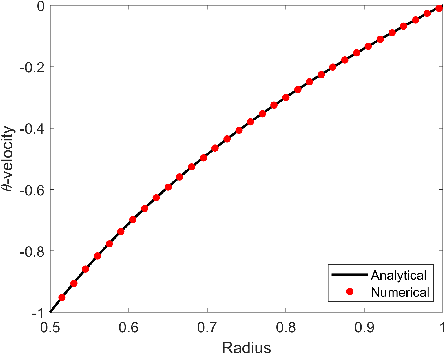
(a)

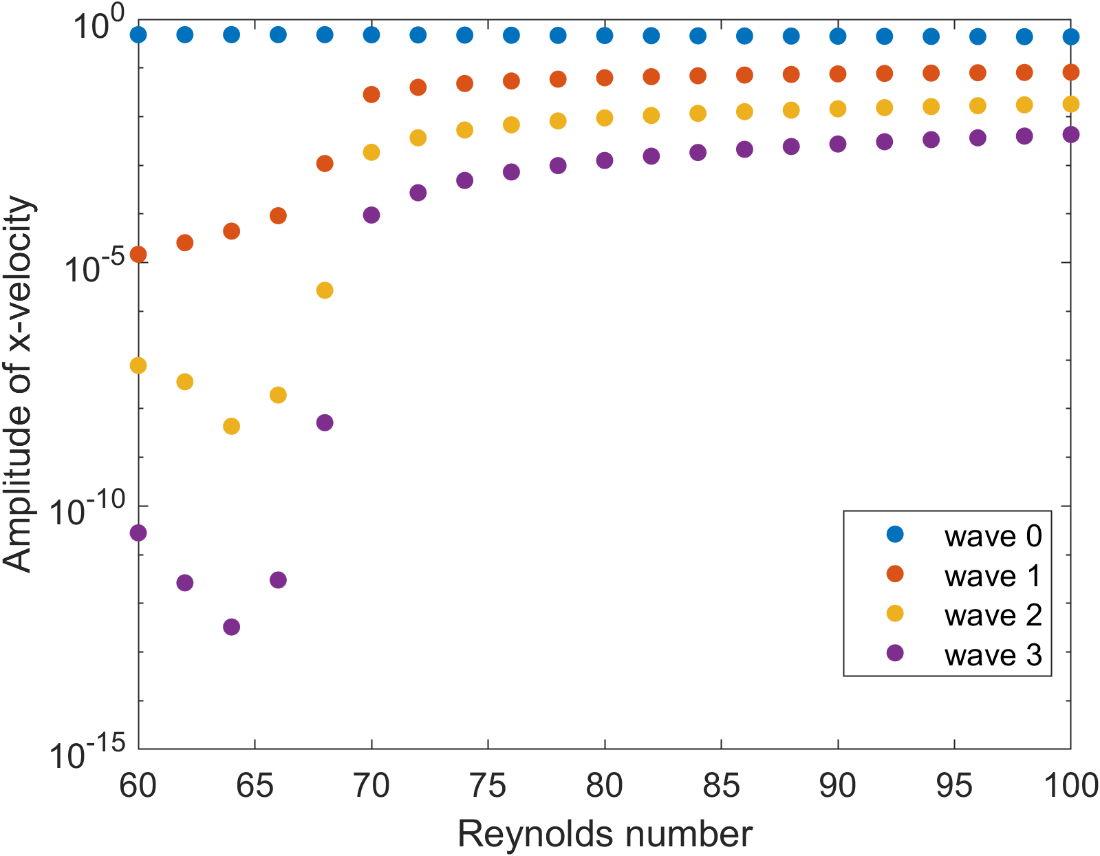
(b)

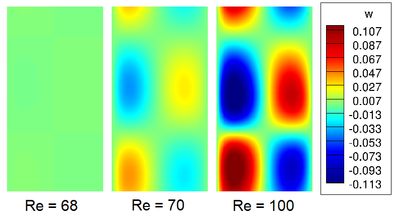
(c)

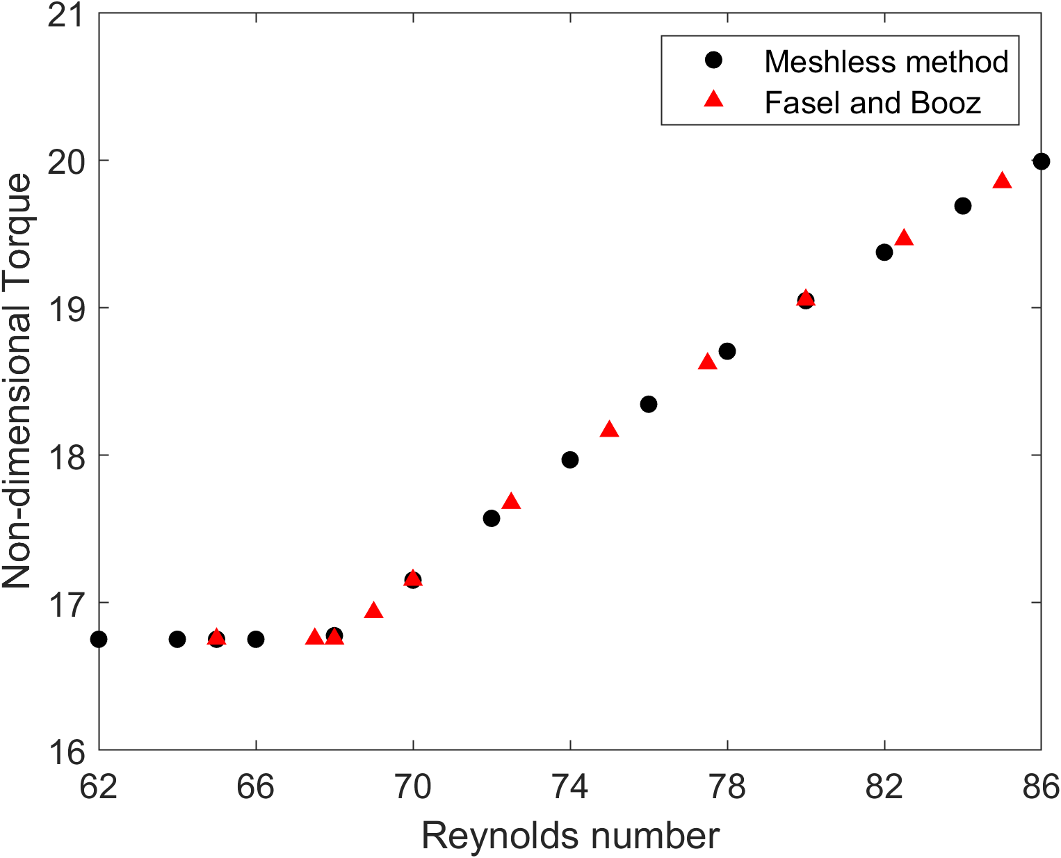
(d)

Figure 2: Plots and contours for validating the code for subcritical and supercritical stages of Taylor Couette setup: a) Comparison of analytical and numerical solution of cylindrical Couette flow data (subcritical stage) taken on a radius length at an axial location of $z=0.5$; b) Plots of four domain averaged amplitudes of x-velocity at several Reynolds numbers. Transition of cylindrical Couette flow to Taylor Couette flow is seen to occur between Reynolds number of 68 and 70; c) Contours of axial velocity in the $r-z$ plane near supercritical Reynolds number; and d) Non-dimensional torque vs Reynolds number plot for circular Taylor Couette flow validated with Fasel and Booz [96]

Calculations of three-dimensional flow in an elliptical enclosure with a rotating inner cylinder were then initiated by first determining the number of scattered points needed for accuracy, and the number of wave modes needed in the axial direction to resolve the streamwise variations of field variables. These grid-independency calculations were performed at $Re=300$, which is slightly below the Reynolds number at which the flow is observed to become unsteady. We use three different sets of scattered points in the cross-sectional plane. In the periodic direction, we consider twenty five modes ($N=25$) and study the energy content as a function of the wave number. The cross-sectional distributions of scattered points (fig. 3) are characterized in terms of average point spacing between adajacent scattered points. The energy content in each wave number is then plotted for the three velocities at eight discrete locations ($r=0.6$, $0.7$, $0.8$, $0.9$ and $\theta=0\degree$, $90\degree$). In fig. 4 we show here four representative plots of the amplitudes of the velocities versus the streamwise wave number. It is seen that the medium point spacing of $0.0158$ gives values very close to those of $\approx 0.008$. Also, the amplitude of the velocities drops below 1.0e-5 for wave numbers greater than $15$. We therefore conclude that the results with point spacing of $\approx 0.0158$ and $15$ wave numbers are sufficiently accurate while computationally economical. The flow is considered steady and converged when the time variations in the variables decrease and stay below 1.0e-5.

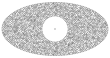
Figure 3: Sample point distribution of 1874 points

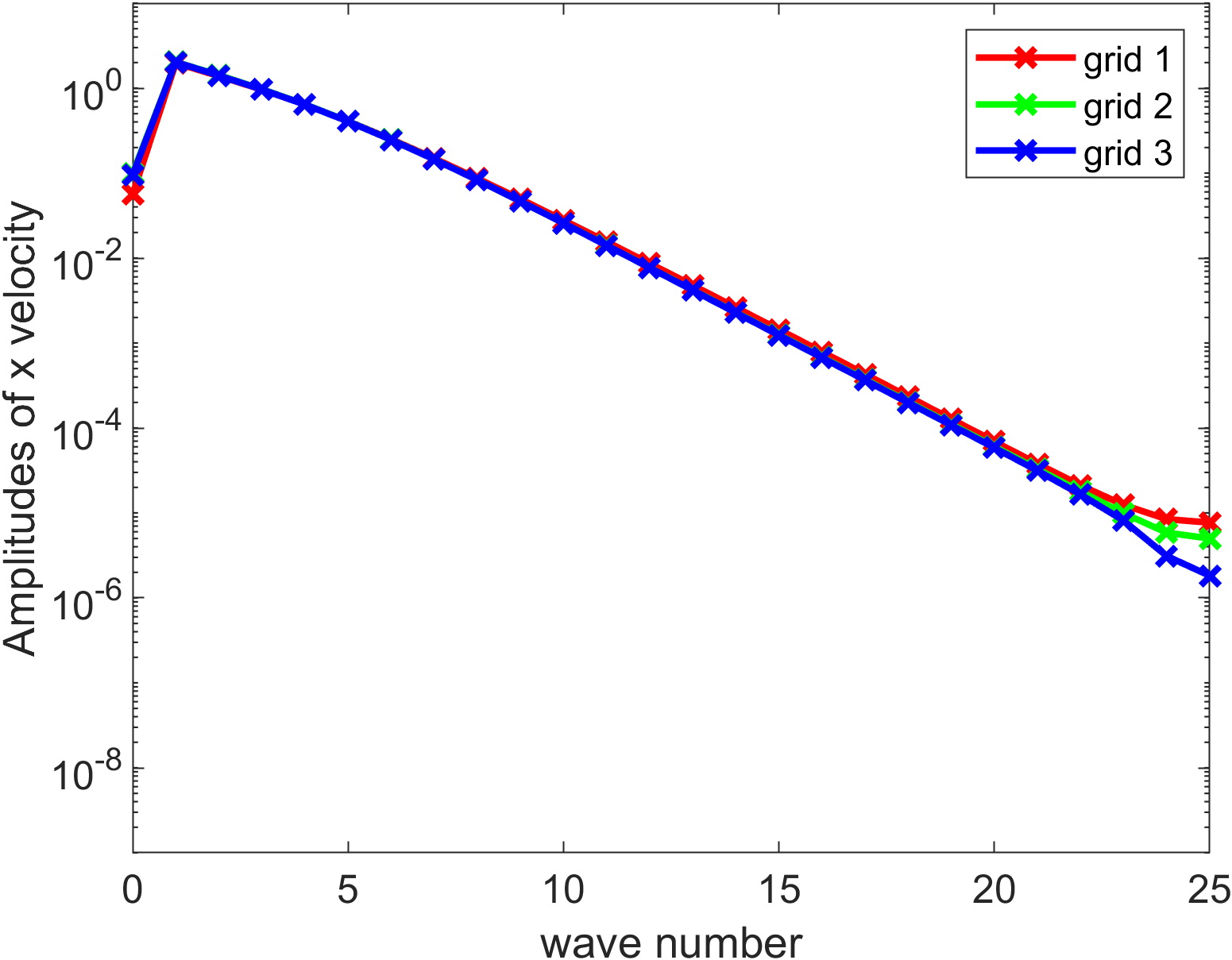
(a)

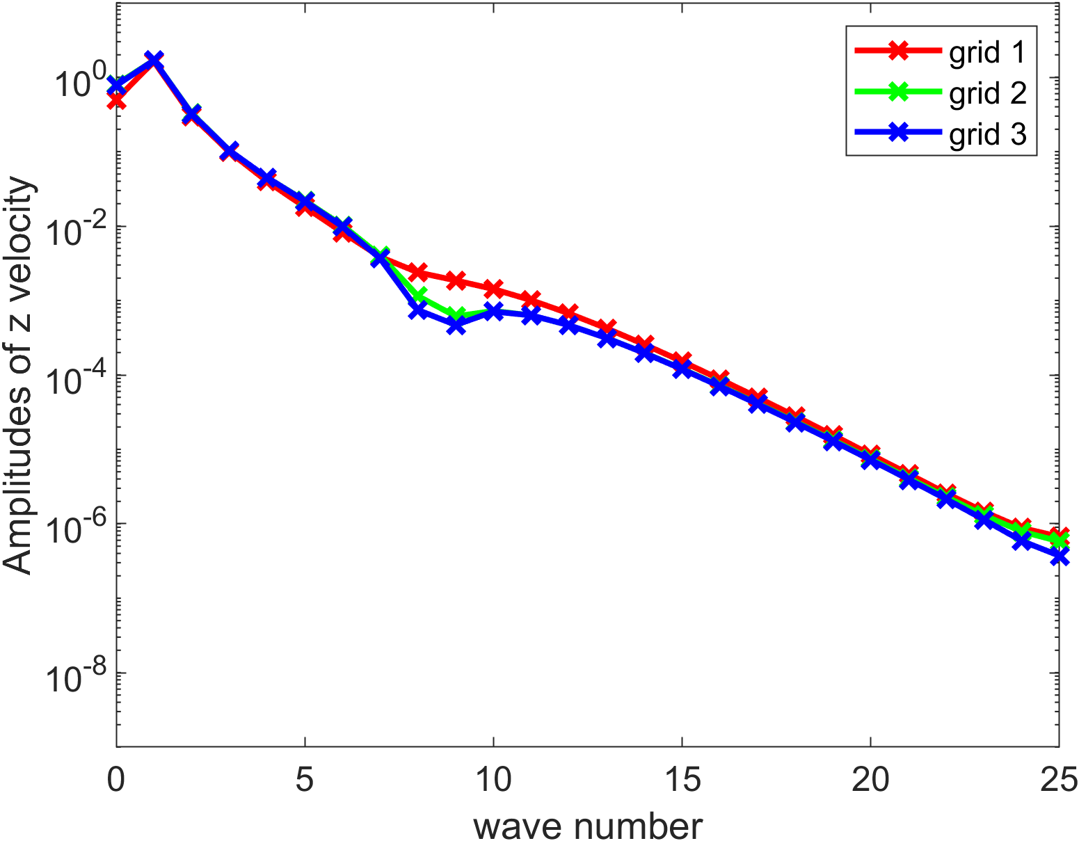
(b)

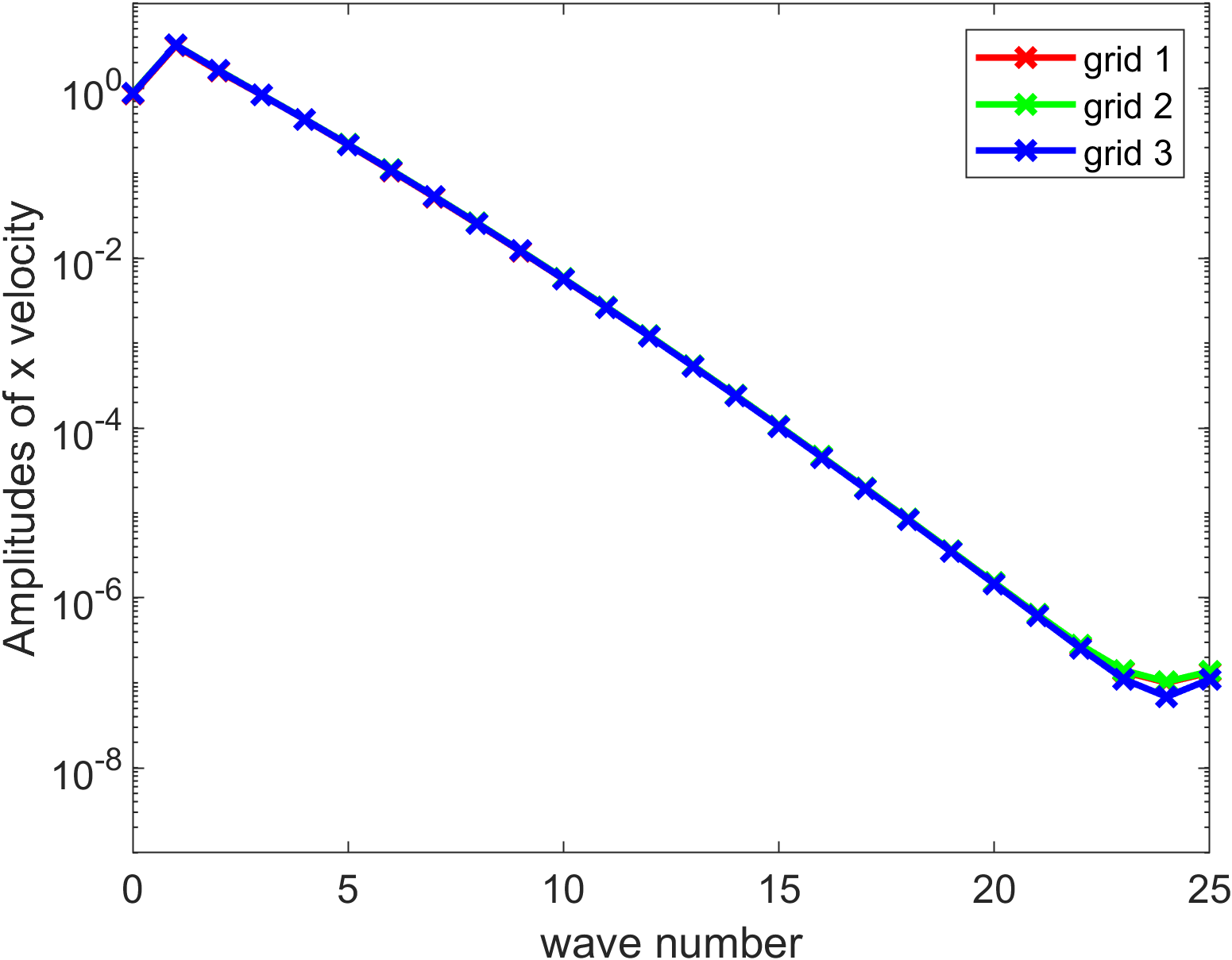
(c)

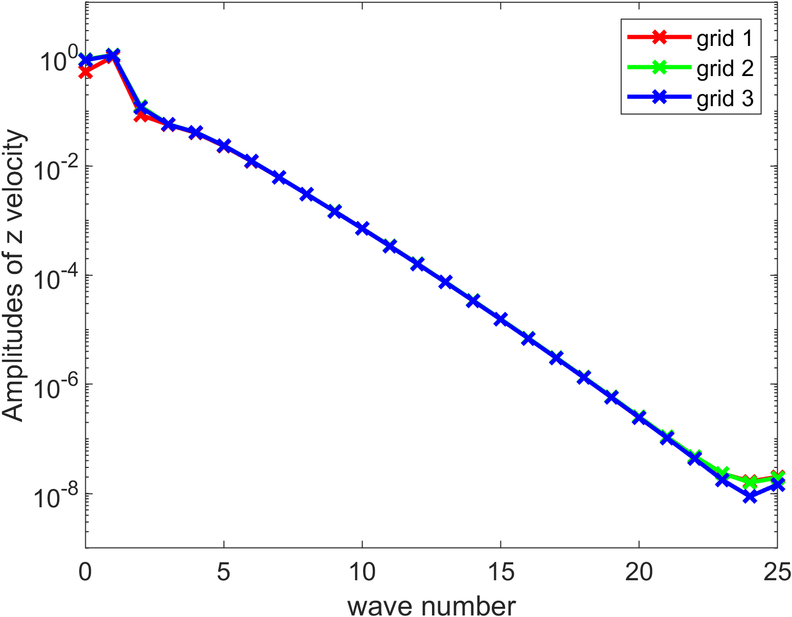
(d)

Figure 4: a) Amplitude of x velocity vs wave number at $\theta=0\degree$ $r=0.7$; b) Amplitude of z velocity vs wave number at $\theta=0\degree$ $r=0.7$; c) Amplitude of x velocity vs wave number at $\theta=0\degree$ $r=0.9$; and d) Amplitude of z velocity vs wave number at $\theta=0\degree$ $r=0.9$;

4 Results for Concentric Inner Cylinder

4.1 Torque and heat transfer rates

Figures 5(a) and 5(b) show the non-dimensional torque and Nusselt number as a function of the Reynolds number. The non-dimensional torque and heat transfer are computed as given in eqs. 4 and 5. From fig. 5(a) we observe that as expected the non-dimensional torque is constant for the subcritical Reynolds numbers and suddenly increases nonlinearly with Reynolds number. In a similar manner, the Nusselt number jumps when transition occurs to a Taylor-Couette flow from a base Couette flow. The base two-dimensional flow was previously presented in [82] where several flow patterns are documented for varying flow and geometric parameters. Both the Nusselt number and the non-dimensional torque have a monotonic increasing trend with Reynolds number once transition to a supercritical state occurs. The transition is seen to occur at a Reynolds number between 70 and 75, although in this study we did not precisely determine its value. Figure 6 plots the amplitudes of the first five oscillatory modes and the zeroth mode for the Reynolds numbers computed. It can be seen that the amplitudes of the oscillatory modes suddenly jump to moderate values at Reynolds number between 70 and 75, consistent with observations of torque and Nusselt number. The values of amplitude in the fig. 6 are not scaled. However to observe the bifurcation, the actual amplitudes are not required. We observe again that the first bifurcation occurs at a Reynolds number between 70 and 75, transitioning from a Couette flow to a Taylor-Couette flow.

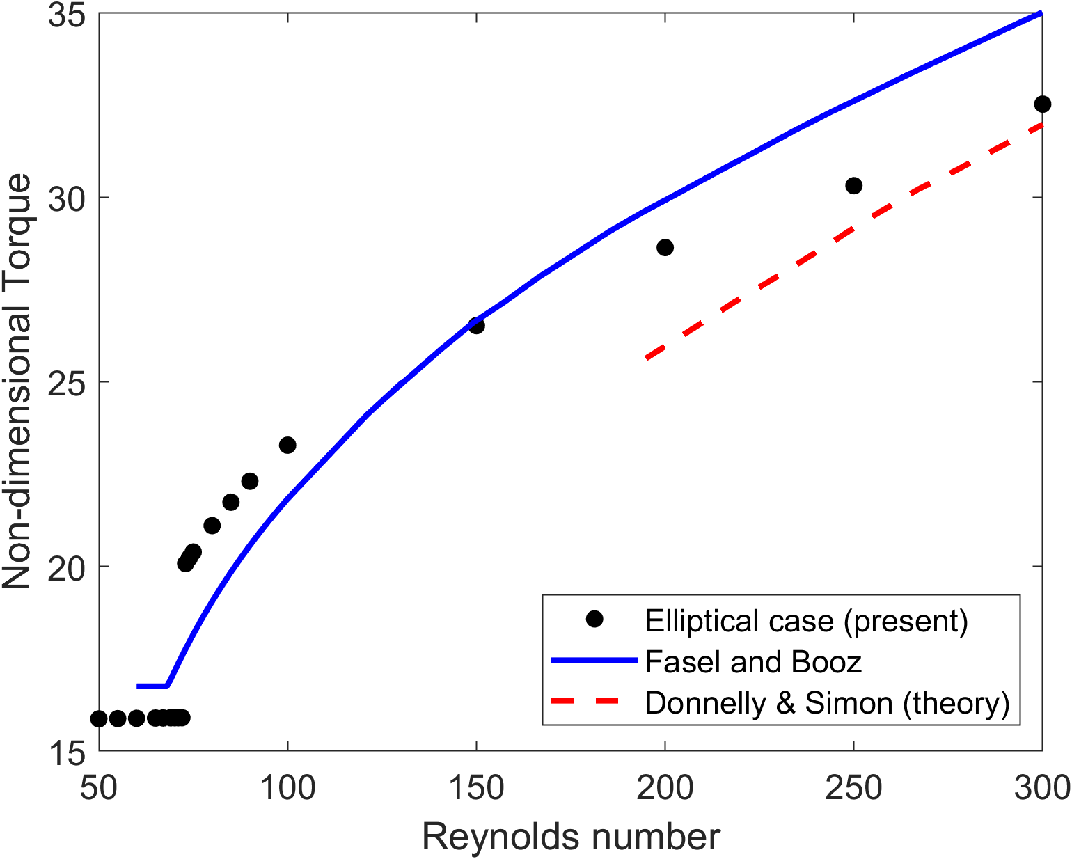
(a)

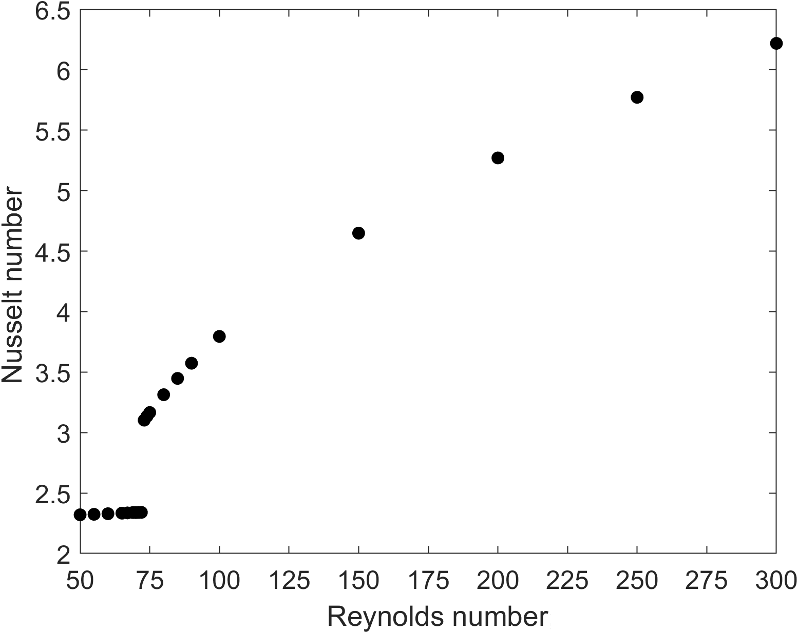
(b)

Figure 5: a) Plot of non-dimensional torque vs Reynolds number for the present case with elliptical outer cylinder in comparison with simple Taylor Couette flow from Donnelly and Simon [97], and Fasel and Booz [96]; and b) Nusselt number vs Reynolds number for the present case

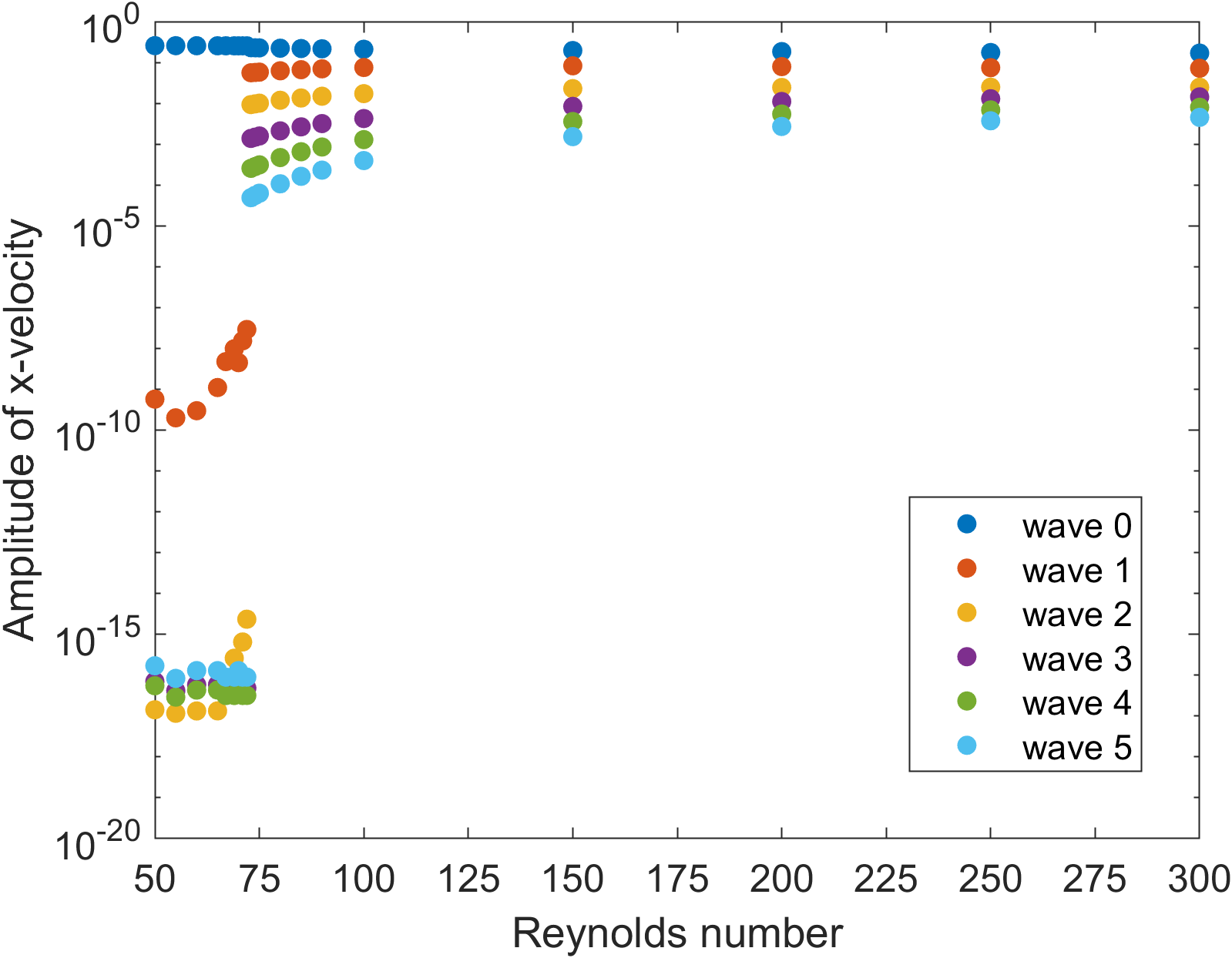
(a)

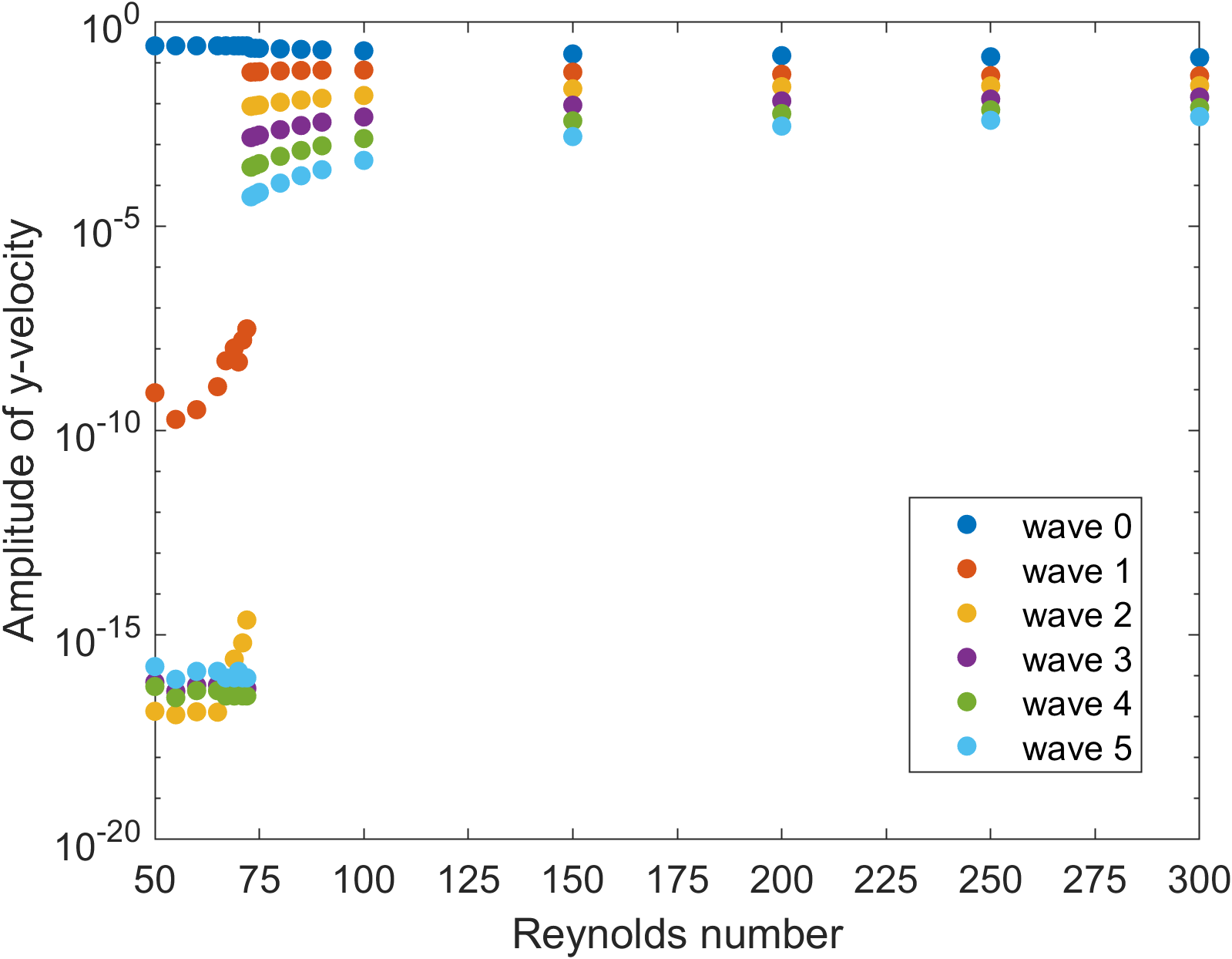
(b)

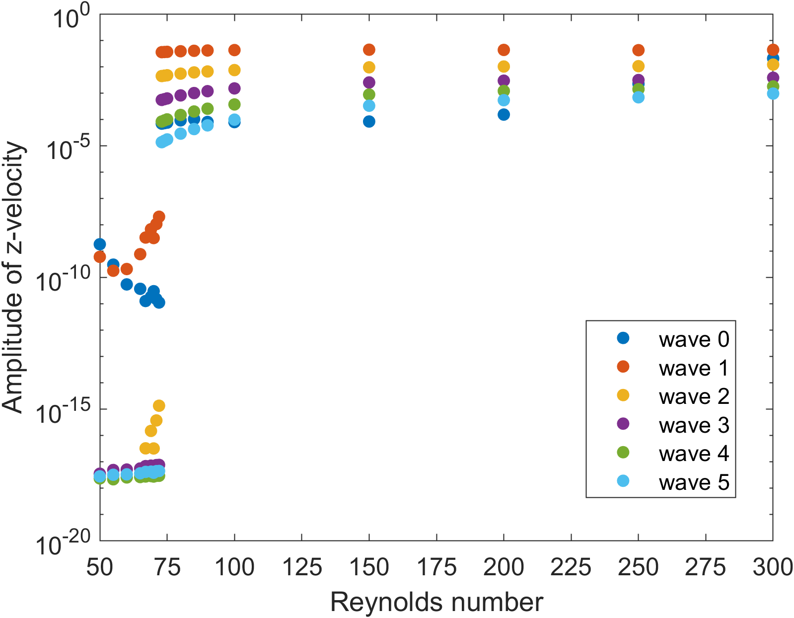
(c)

Figure 6: Plots of amplitudes of first six Fourier modes averaged over the entire domain for the three velocity components against Reynolds number: a) averaged amplitude of the x-velocity vs Reynolds number; b) averaged amplitude of the y-velocity vs Reynolds number; c) averaged amplitude of the z-velocity vs Reynolds number

4.2 Plots of streamlines

In figs. 7, 8, 9 and 10, we present the streamlines for progressively increasing Reynolds numbers from 70 to 300 (the flow is seen to be steady at all these Reynolds numbers). Below the critical Reynolds number, the streamlines show an outward flow along the semi-major axis and an inward flow along the semi-minor axis. This is due to the expansion and contraction of the flow as it squeezes into the smaller gap and then expands to the larger cross-sectional area. The inward streamlines reflect a secondary vortex formed by the shear of the primary rotating flow caused by the rotating cylinder. We observe the same patterns for Re = 50, 60 and 70. The first Reynolds number where the Taylor vortices appear is 75, although they may have developed at a slightly smaller Reynolds number. At Re = 75 and beyond, the streamlines in the ($r-z$) plane show the formation of Taylor cells. As in the case of concentric circular cylinders, a periodic pair of counter-rotating vortices is formed with a height equal to the width of the smaller gap (at the minor axis). However, the vortices are no longer axisymmetric (as in the case of circular cylinders), but expand and contract between the major and minor axes of the ellipse. It can be seen that on the semi-major axis, the vortex occupies the entire gap with a vortex height of $0.5$ and a width of $1.0$ units. In the direction of the minor axis however, the cell is more of a square shape with width and height of $0.5$. The expansion of the Taylor cells into the larger gap is evident from these ($r-z$) plane plots.

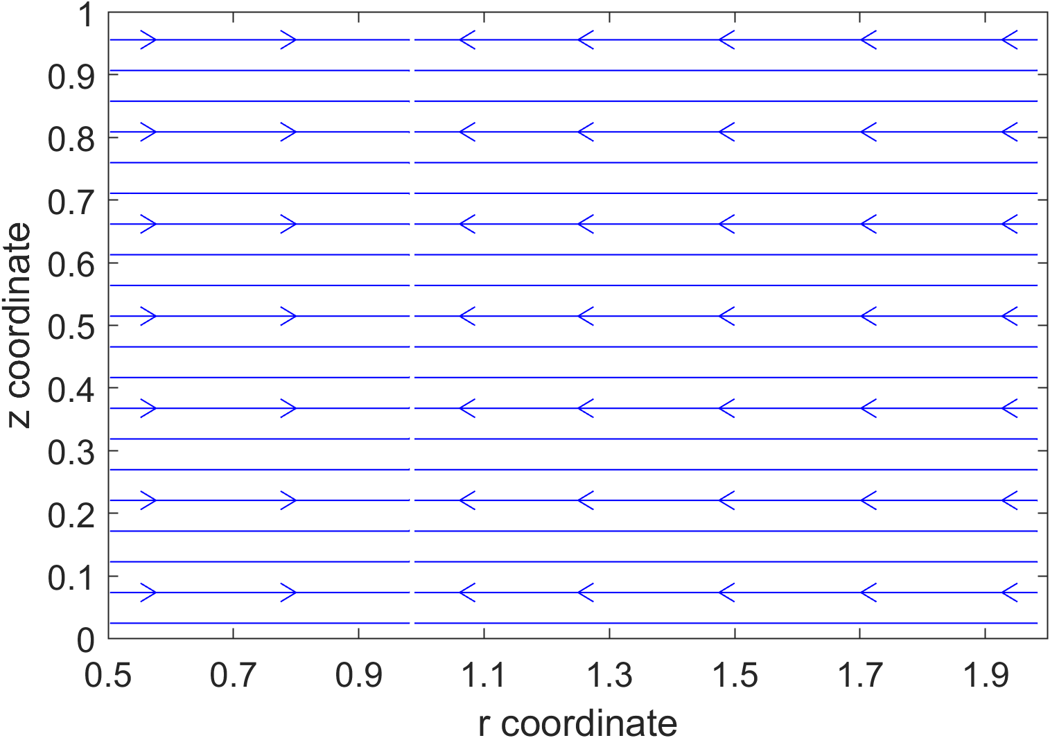
(a)

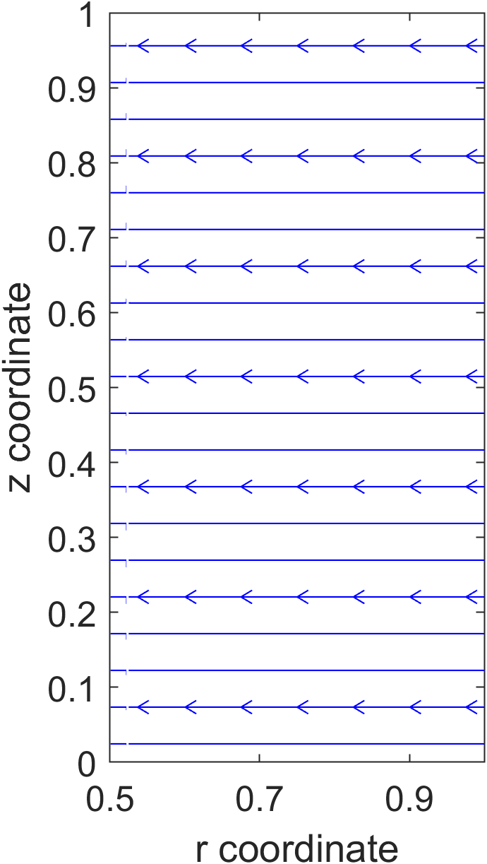
(b)

Figure 7: Streamlines in a section along: a) the semi-major axis; b) the semi-minor axis; for Re = 70

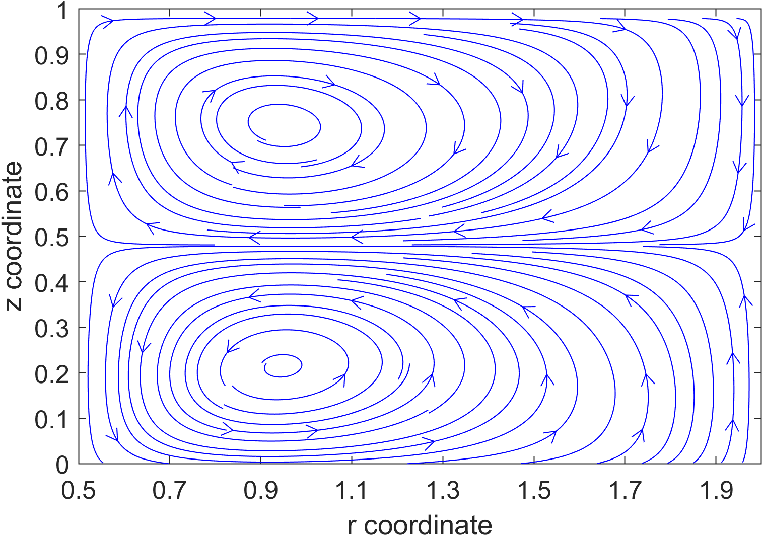
(a)

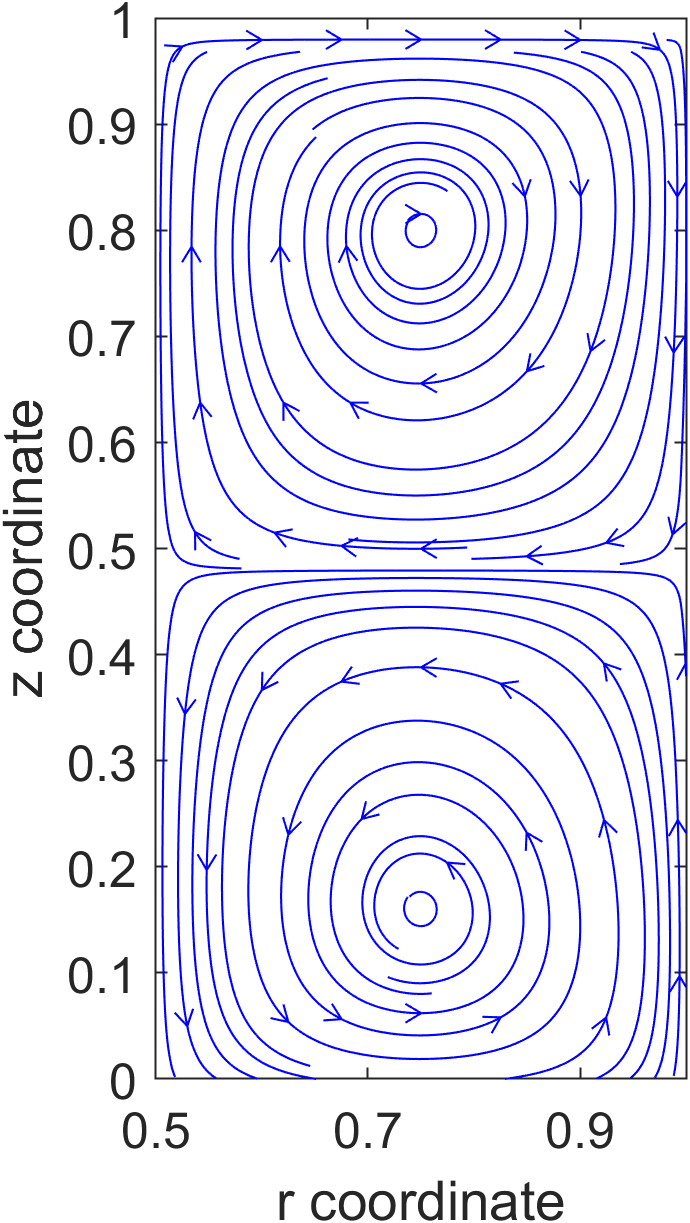
(b)

Figure 8: Streamlines in a section along: a) the semi-major axis; b) the semi-minor axis; for Re = 75

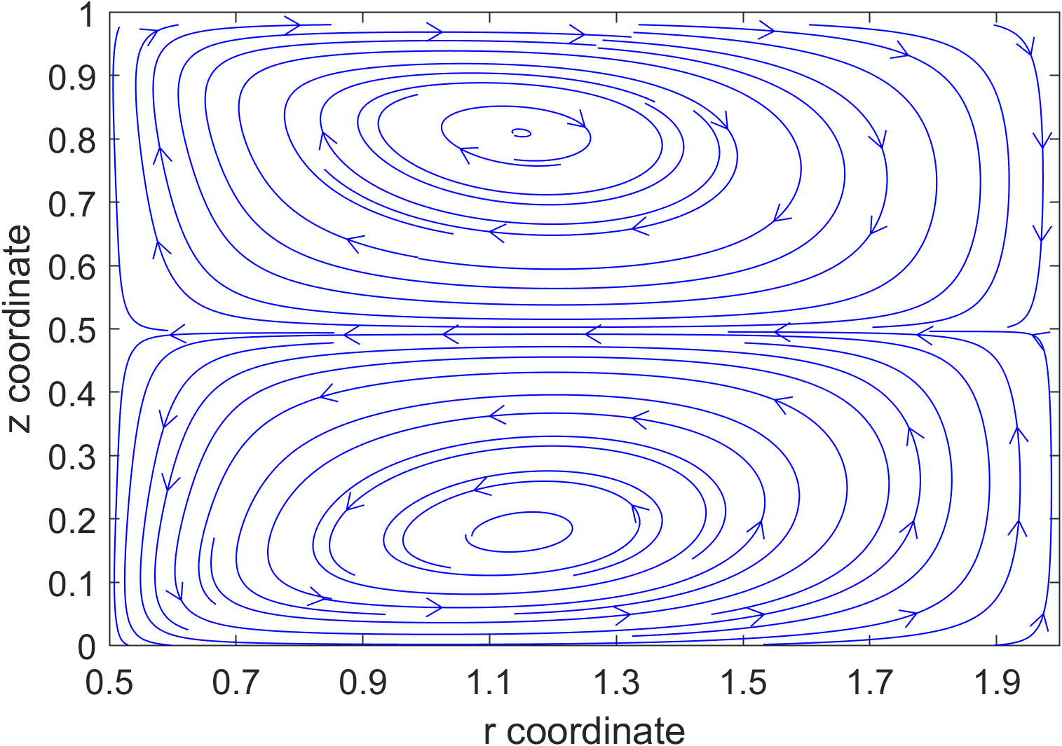
(a)

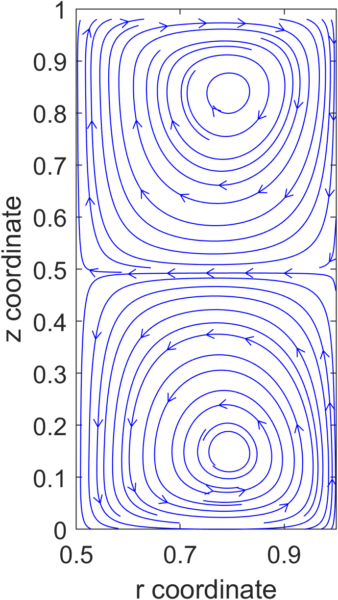
(b)

Figure 9: Streamlines in a section along: a) the semi-major axis; b) the semi-minor axis; for Re = 200

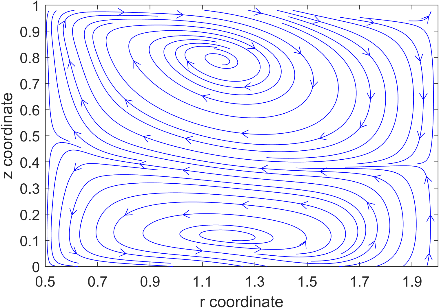
(a)

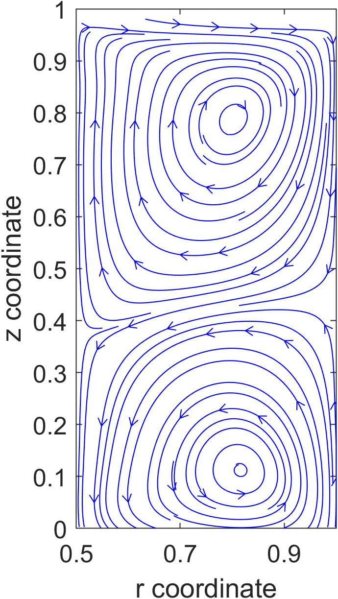
(b)

Figure 10: Streamlines in a section along: a) the semi-major axis; b) the semi-minor axis; for Re = 300

4.3 Axial velocity distributions

4.3.1 Contours of axial velocity in r-z planes

Figures 11 and 12 show the contours of axial velocity in ($r-z$) planes cutting the major and minor axes for four of the several Reynolds numbers computed. The plots reveal the same structure of the Taylor cells shown by the plots of streamlines but now indicate the magnitudes of the axial velocities. The pair of vortices show the upward and downward motion of the flow. As seen earlier, there is no axial flow at Reynolds number below 75. At Re = 75, we first notice the appearance of the Taylor cells. This value of Reynolds number is close to the value also observed for concentric circular cylinders. We notice that along the major axis, the center of the Taylor cells is located approximately at r = 0.95. The downward axial flow traverses radially and reaches the outer wall and occupies the entire gap. We see only one single Taylor cell which is elongated in the radial direction along the major axis. At the outer wall, the radial flow turns upwards and flows to the inner wall. This pattern is the opposite for the clockwise rotating cell. As the flow occupies the outer wall region, the axial velocities become smaller because of the larger area for the flow. As the Reynolds number is increased, the Taylor cells get somewhat distorted, and the centers of the cells move closer to the outer wall ($r\approx 1.1$). The cells continue to distort with increase in Reynolds number and at $Re=300$, the flow transitions to a complex structure. We observe that the flow is however still steady at this Reynolds number. Figure 12 shows the results for the plane cutting the minor axis of the ellipse. Here, the gap is $0.5$ only and the cell structure resembles the circular cylinder case. Even at $Re=300$, the cells appear well-structured. Note that the Reynolds number is defined by the gap at the minor axis, hence the Reynolds number defined by the gap along the major axis will be three times larger. Hence the flow in the major axis gap may have transitioned to some form of spiral vortices.

(a) Re = 70

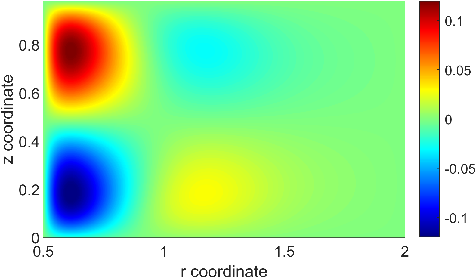
(b) Re = 75

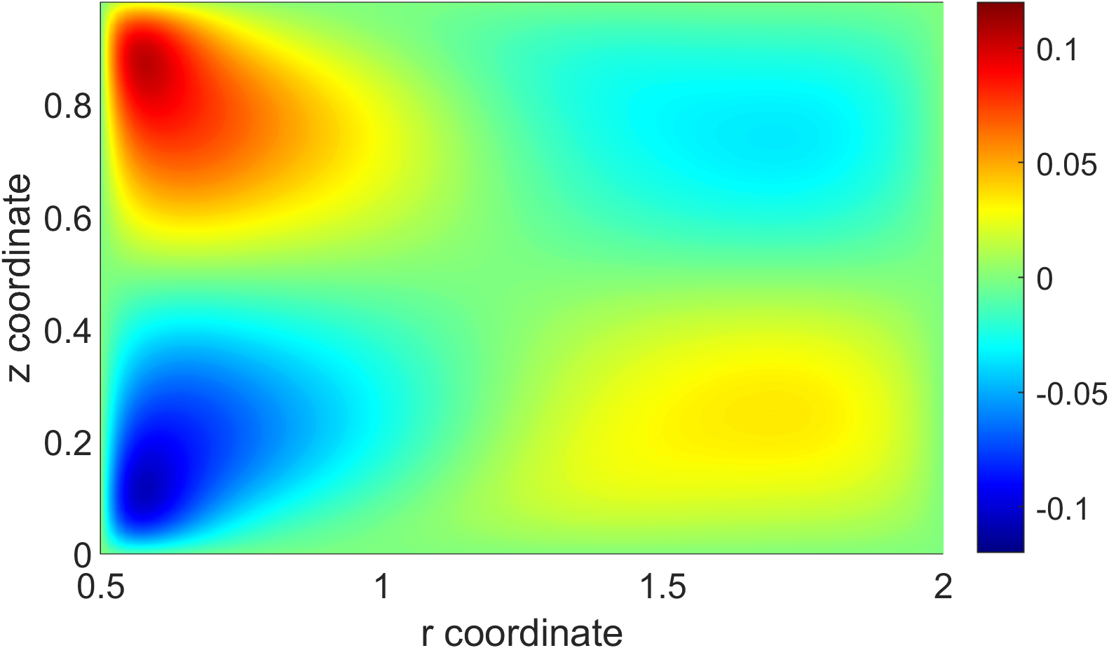
(c) Re = 200

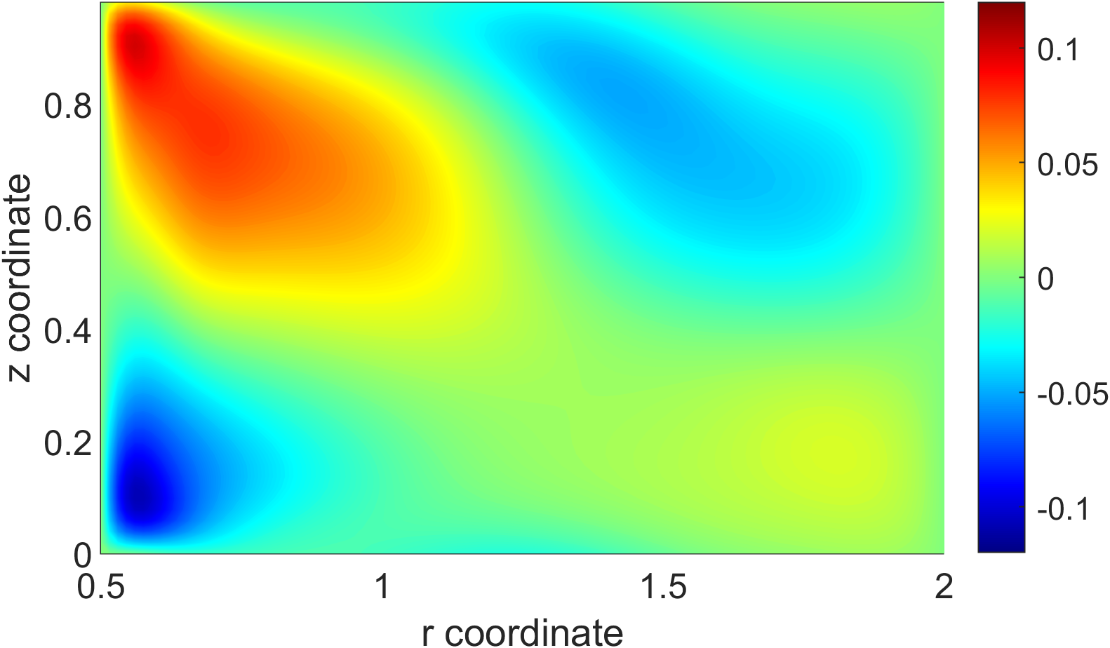
(d) Re = 300

Figure 11: Contours of axial velocity in the plane along semi major axis of ellipse

(a) Re = 70

(b) Re = 75

(c) Re = 200

(d) Re = 300

Figure 12: Contours of axial velocity in the plane along semi minor axis of ellipse

4.3.2 Contours of axial velocity in z-$\theta$ planes: $r=0.8$

Figure 13 show the contours of axial velocity in the ($z-\theta$) planes. We have arbitrarily selected a radius of $0.8$ ($r_{i}=0.5$, $b=1.0$, and $a=2.0$) and plot the contours of the axial velocity. For $Re=75$, the first Re considered in the super-critical region, we see alternate regions of positive and negative velocities. This contrasts with horizontal bands throughout the $\theta$ space seen for the concentric circular cylinder case. The alternate regions are due to the shift in the vortex centers as the Taylor cells move from the major to the minor gaps. We have plotted the contours for $r=0.8$, which corresponds to the left of the vortex center in the major gap with upward (positive) velocity above $z=0.5$ and negative axial velocity below around $z=0.5$. However, in the minor gap, the center of the vortex moves closer to $r=0.75$ (center of the gap) and therefore at $r=0.8$, a downward flow in the upper region and a upward flow in the region below is seen. It is still one single toroidal vortex with the toroid converging and diverging between the major and minor gaps. Because we have considered a constant absolute radius, we observe these alternating patterns. The same patterns are seen for $Re=100$ (not shown here) and for $Re=200$. For $Re=300$, the above pattern gets distorted with break-up of the cell structure. As mentioned earlier, this may be a prelude to the onset of unsteadiness in the flow, although the flow at $Re=300$ converged to a steady state.

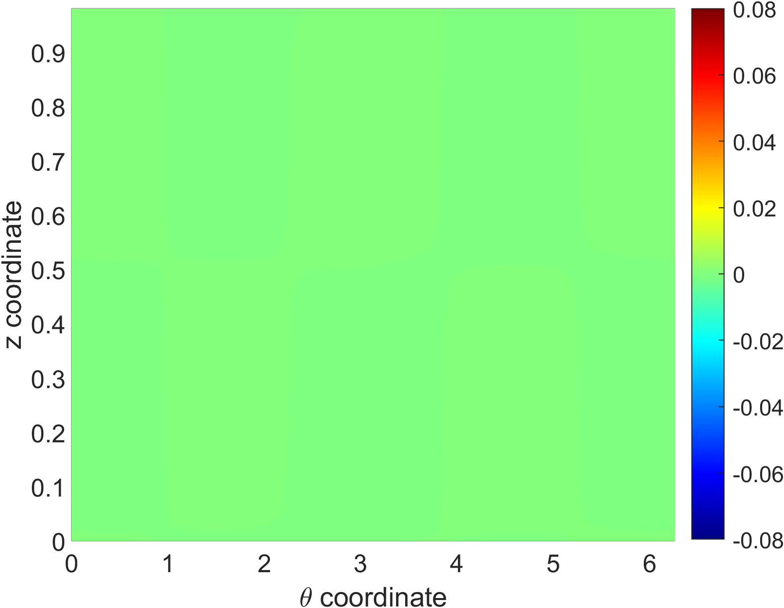
(a) $Re=70$

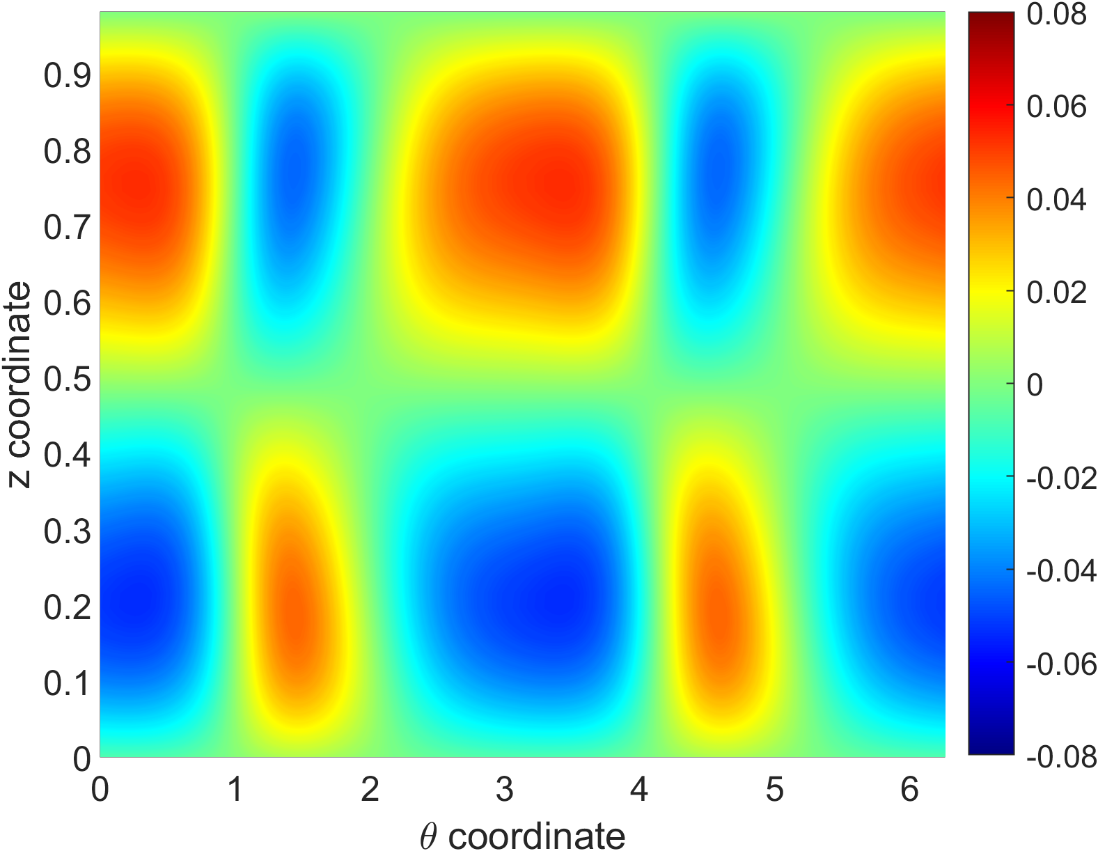
(b) $Re=75$

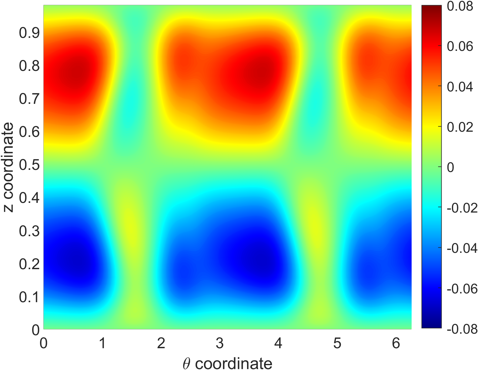
(c) $Re=200$

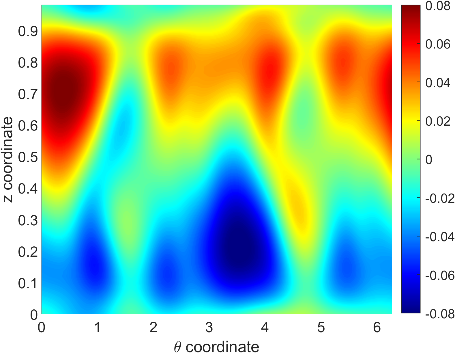
(d) $Re=300$

Figure 13: Contours of z-velocity for different Reynolds numbers in a constant radius plane where radius, $r=0.8$

4.3.3 Contours of axial velocity in r-$\theta$ planes

Figures 15(a), 16(a) and 17(a) show contours of axial velocities in three constant z planes ($r-\theta$) for $Re=75$. As expected, the Taylor cells are mirror symmetric about the vertical plane, but are antisymmetric about the horizontal plane. The plots for $Re=200$ (figs. 15(b), 16(b) and 17(b)) show similar features as for $Re=75$. However, we observe small amounts of distortion of the inner concentric flow, accompanied by longer ‘tongues’ in the flow along the outer walls. With increase of Reynolds number to $300$ (figs. 15(c), 16(c) and 17(c)), the inner rotating flow gets further distorted with also changes in the outer tongues. These distortions again point to the forthcoming unsteadiness in the flow beyond $Re=300$. The flow has also lost symmetry (mirror symmetry) about the vertical (horizontal) axes.

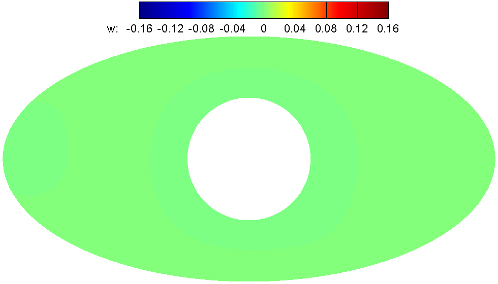
Figure 14: Contour of axial velocity for a subcritical Reynolds number of 70

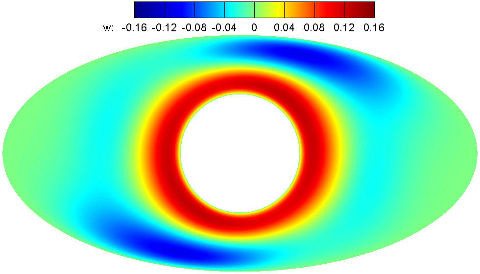
(a) Re = 75

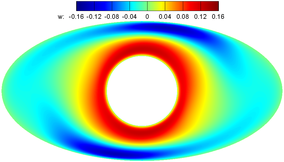
(b) Re = 200

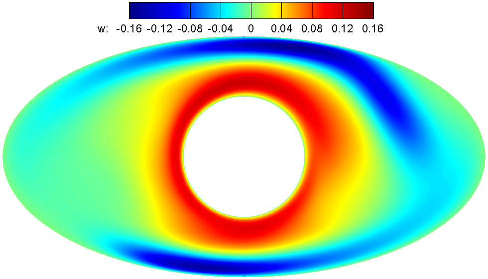
(c) Re = 300

Figure 15: Mid-section cutting through the center of Taylor cell rotating clockwise for supercritical stage

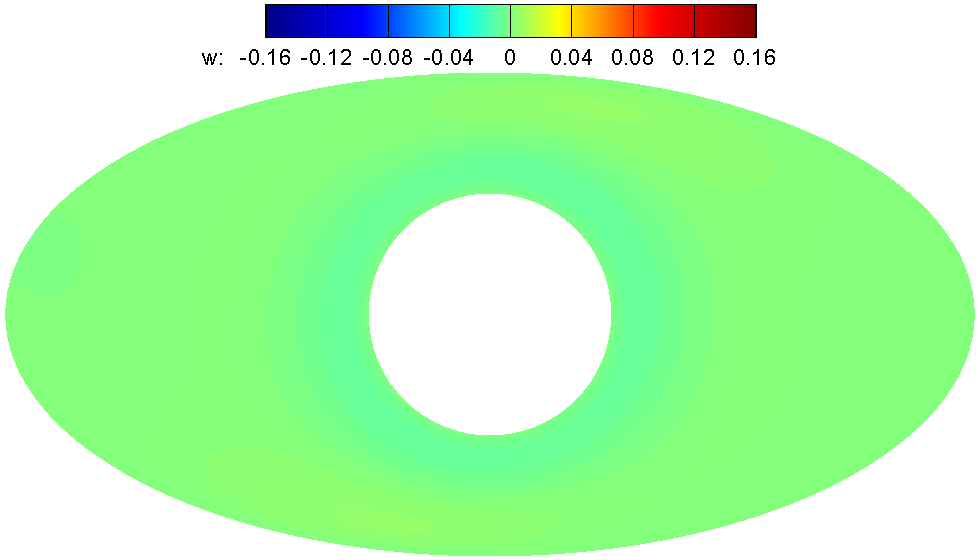
(a) Re = 75

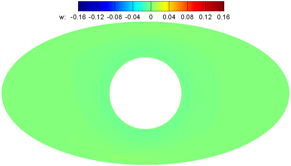
(b) Re = 200

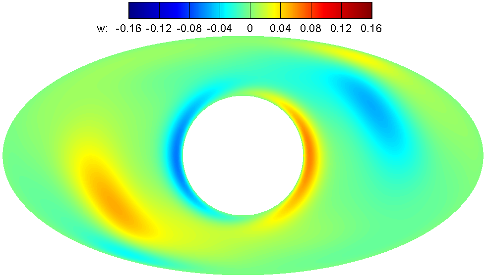
(c) Re = 300

Figure 16: Section between Taylor cells for supercritical stage

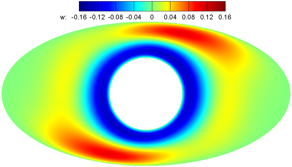
(a) Re = 75

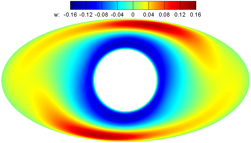
(b) Re = 200

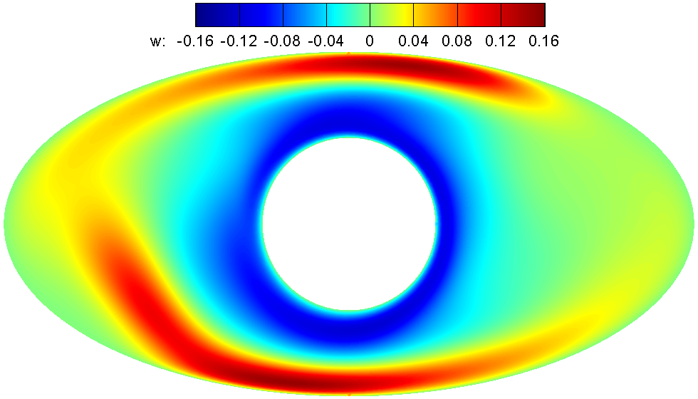
(c) Re = 300

Figure 17: Mid-section cutting through the center of Taylor cell rotating counter clockwise for supercritical stage

4.3.4 Isosurfaces of axial velocity

Figures 18 and 19 present the isosurfaces of axial velocity for different supercritical Reynolds number. The tubular structures are isosurfaces of axial velocity for two different velocities alternately being $+0.005$ and $-0.005$ respectively. Two of them together constitutes on Taylor cell. The Taylor cells appear to be shifting to a wavy structure as Reynolds number changes from 200 to 300. This is more pronounced in the view on minor axis section as in fig. 19. There is a small pinching of the tubular structures seen in fig. 18, as they cross the mid section. This is the location where the fluid exits the small gap area where the pressure is higher. Fenstermacher et al. [7] has observed higher order instabilities as the oscillations and twisting of Taylor vortex cells in simple Taylor Couette flow before they transition to turbulence. The first transition from Taylor vortex is to the wavy vortex flow, characterised by waviness in azimuthal direction. We observe twist and oscillations, characteristics of wavy vortex flow, in the elliptical case as can be observed in fig. 19(d) for a Reynolds number of 300. From here the flow becomes unsteady as the Reynolds number reaches 350. Turbulent cases are not simulated in this study.

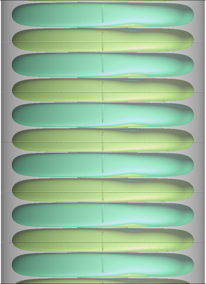
(a) Re = 75

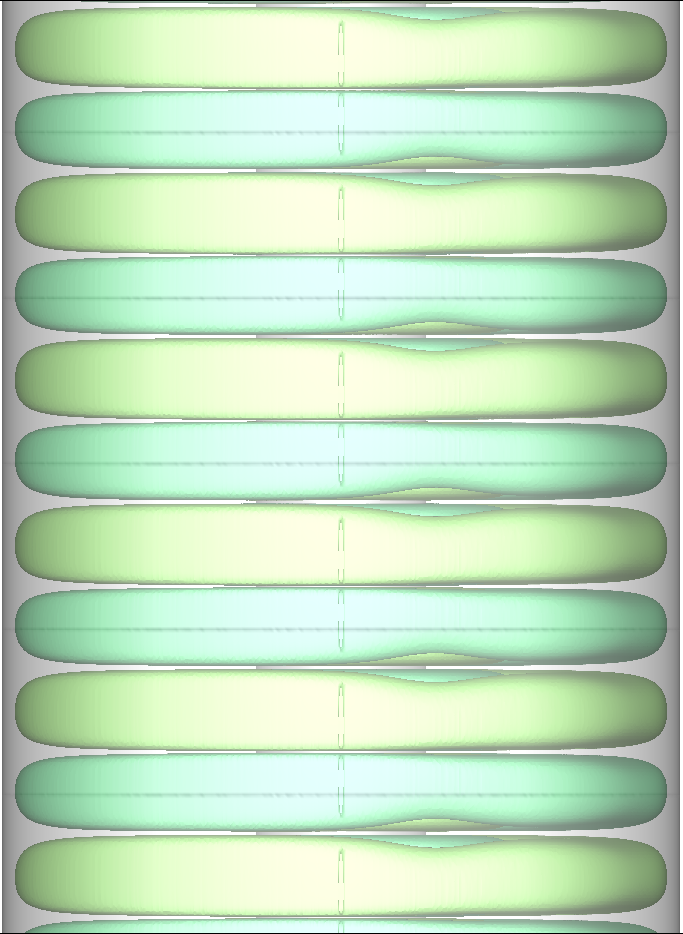
(b) Re = 100

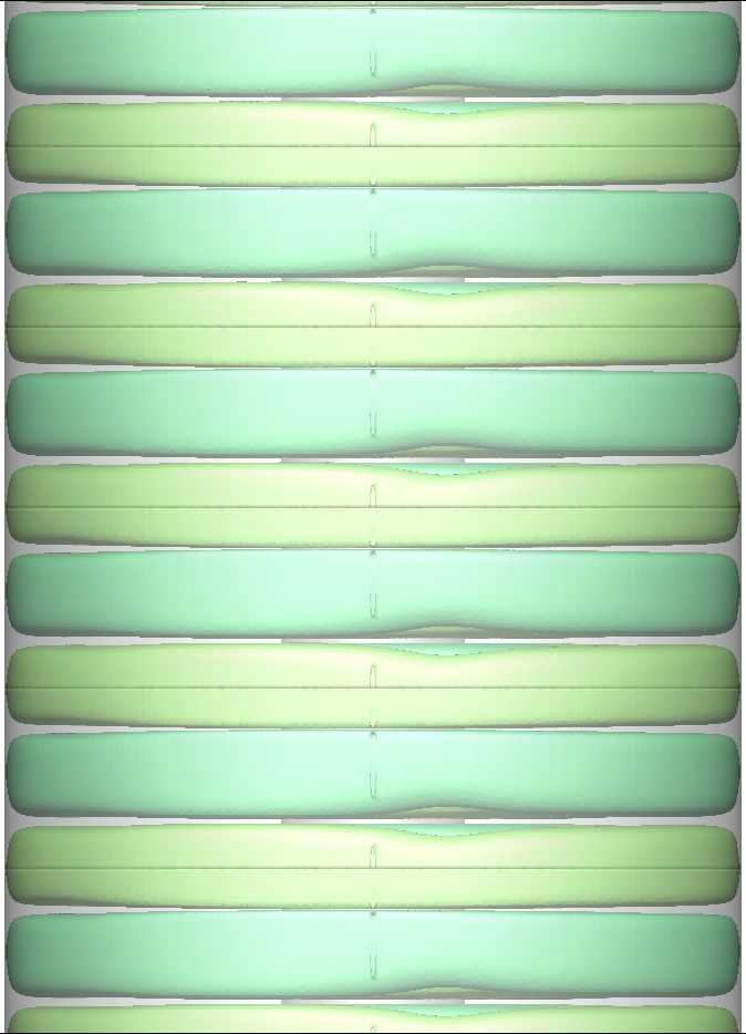
(c) Re = 200

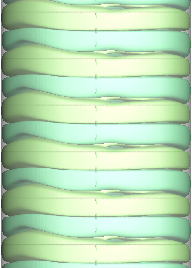
(d) Re = 300

Figure 18: Isosurfaces of axial velocity for $w=\pm 0.005$ viewed from $x-z$ plane (view on the major axis section of ellipse)

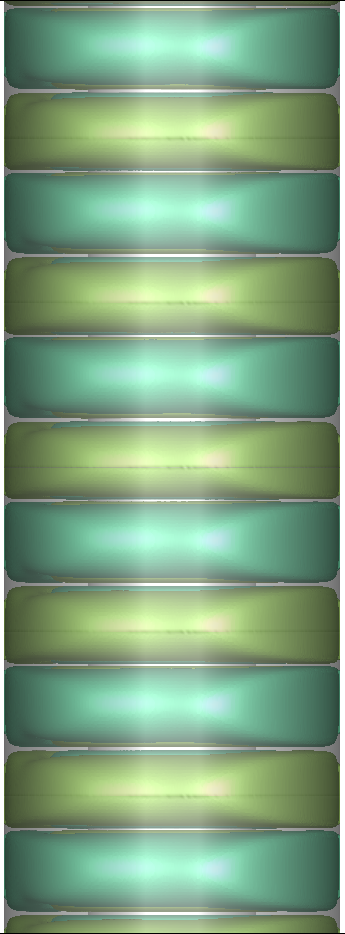
(a) Re = 75

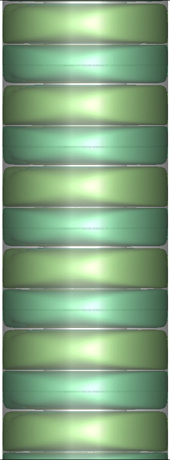
(b) Re = 100

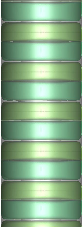
(c) Re = 200

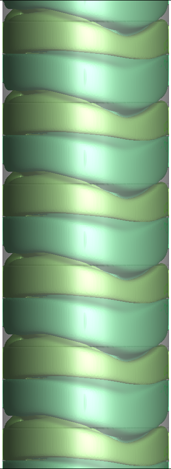
(d) Re = 300

Figure 19: Isosurfaces of axial velocity for $w=\pm 0.005$ viewed from $y-z$ plane (view on the minor axis section of ellipse)

4.4 Pressure distributions

4.4.1 Contours of pressure in r-z planes

At subcritical Reynolds numbers, the pressure distribution is primarily due to the rotational flow. For the concentric Couette flow at subcritical Reynolds number, the distribution is axisymmetric and one-dimensional. However, for the case of the elliptical outer cylinder, the pressure distribution is non-axisymmetric and two-dimensional. As the Reynolds number increases to the supercritical value, a three-dimensional pressure distribution consistent with the velocity distribution and the streamlines evolves. Figures 20 and 21 show the pressure distributions in the ($r-z$) plane along the semi-major and semi-minor axes, along with the velocity vectors. At subcritical $Re=70$, the pressure varies only with radius as there are no Taylor cells. When the Taylor cells form at $Re=75$ and beyond, the pressure on the inner cylinder distorts to increase at the dividing point between the lower and upper vortices. The higher pressure moves the downward and upward moving flows radially towards the inner cylinder. As shown for the axial-velocity contours, the pressure contours (and velocity vectors) become distorted at $Re=300$. Until such a $Re$, the flow in the semi-major ($r-z$) plane is very much well-structured. The pressure distributions shown in the semi-minor ($r-z$) planes are comparatively well structured even at $Re=300$. The higher pressure occurs at $z$ around $0.5$ which is the junction of the upward and downward flow.

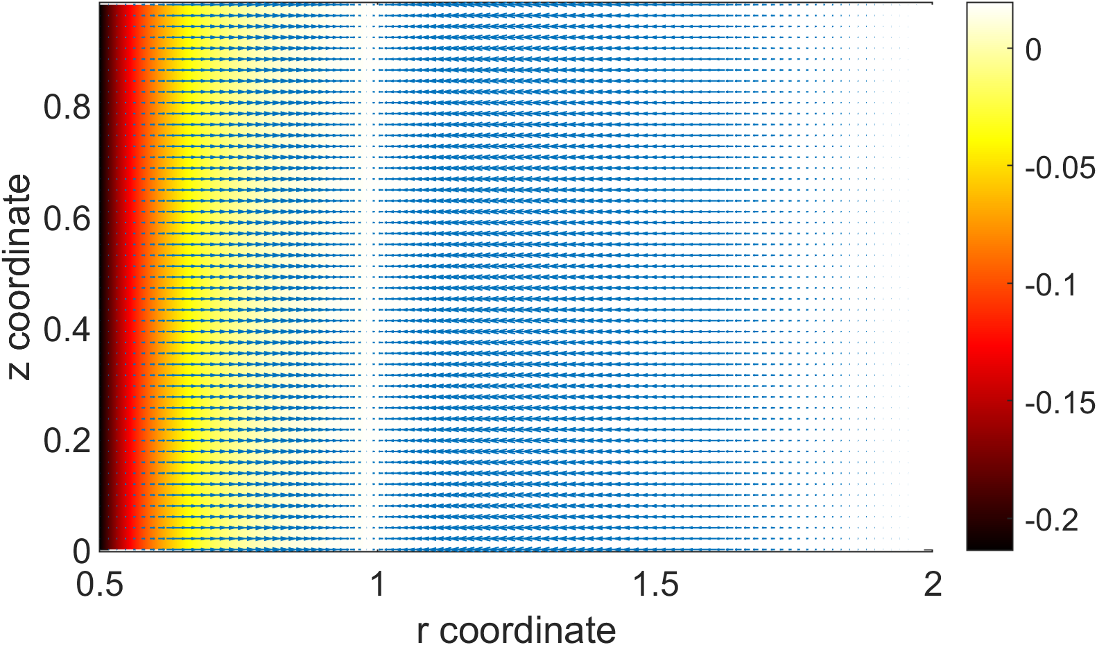
(a) Re = 70

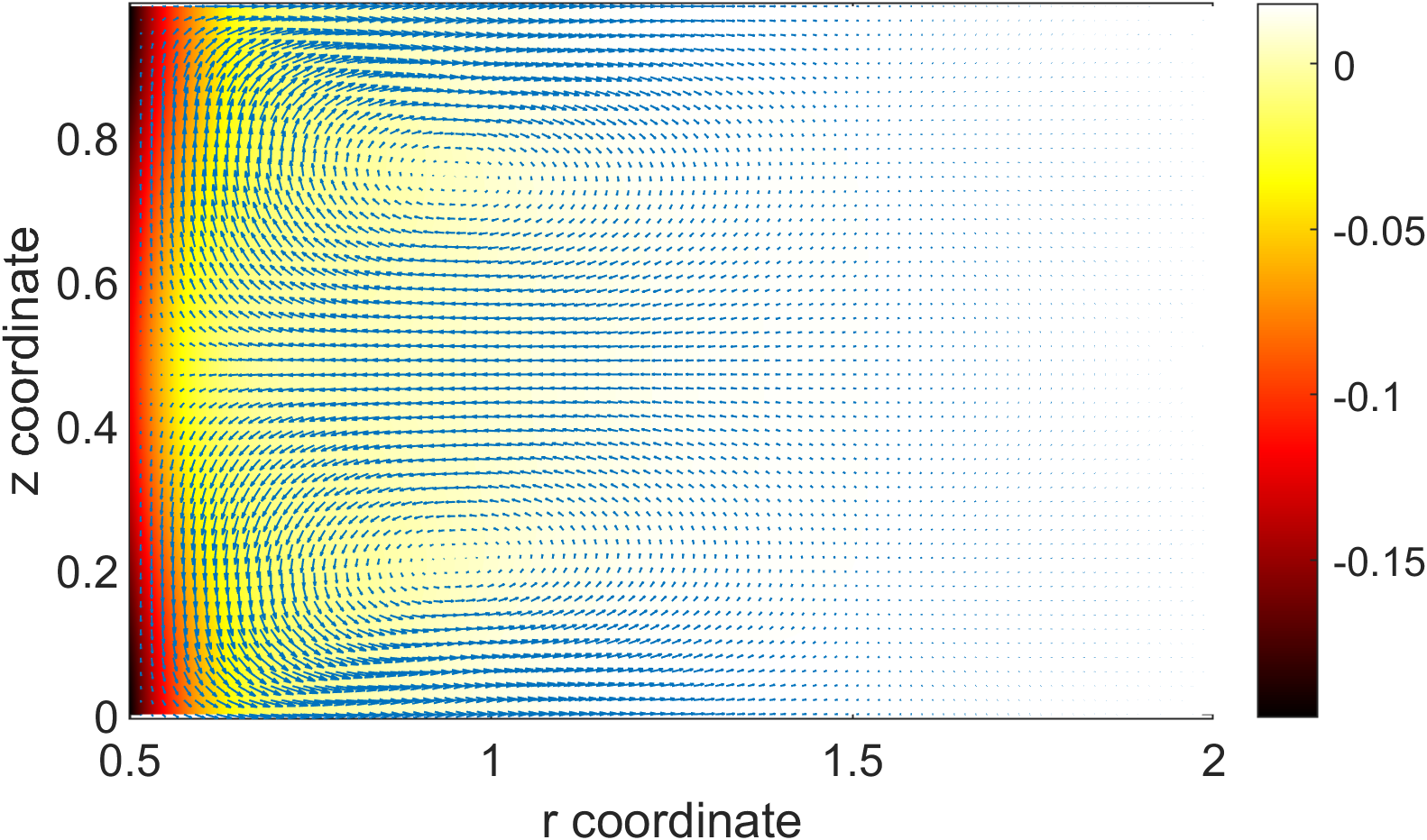
(b) Re = 75

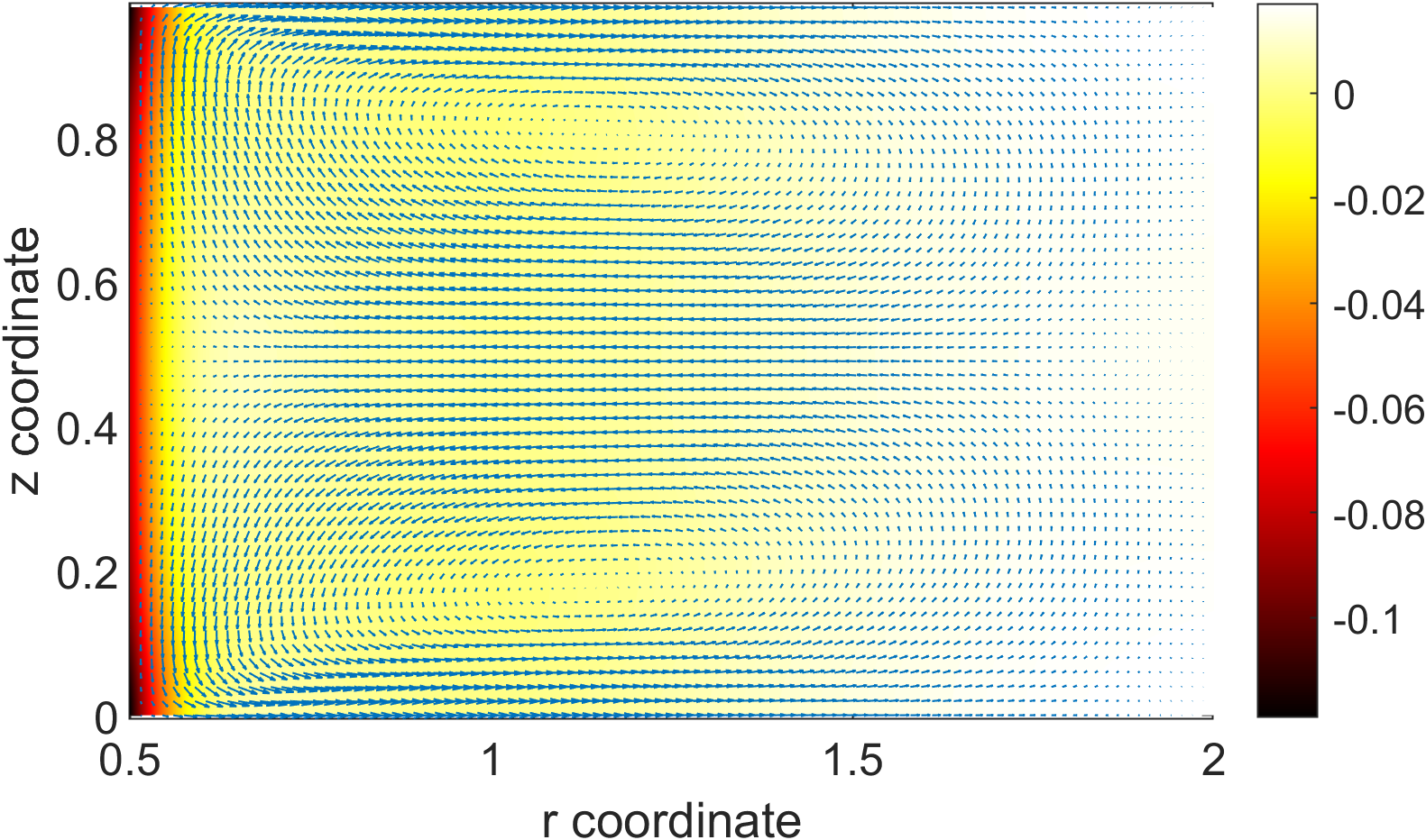
(c) Re = 200

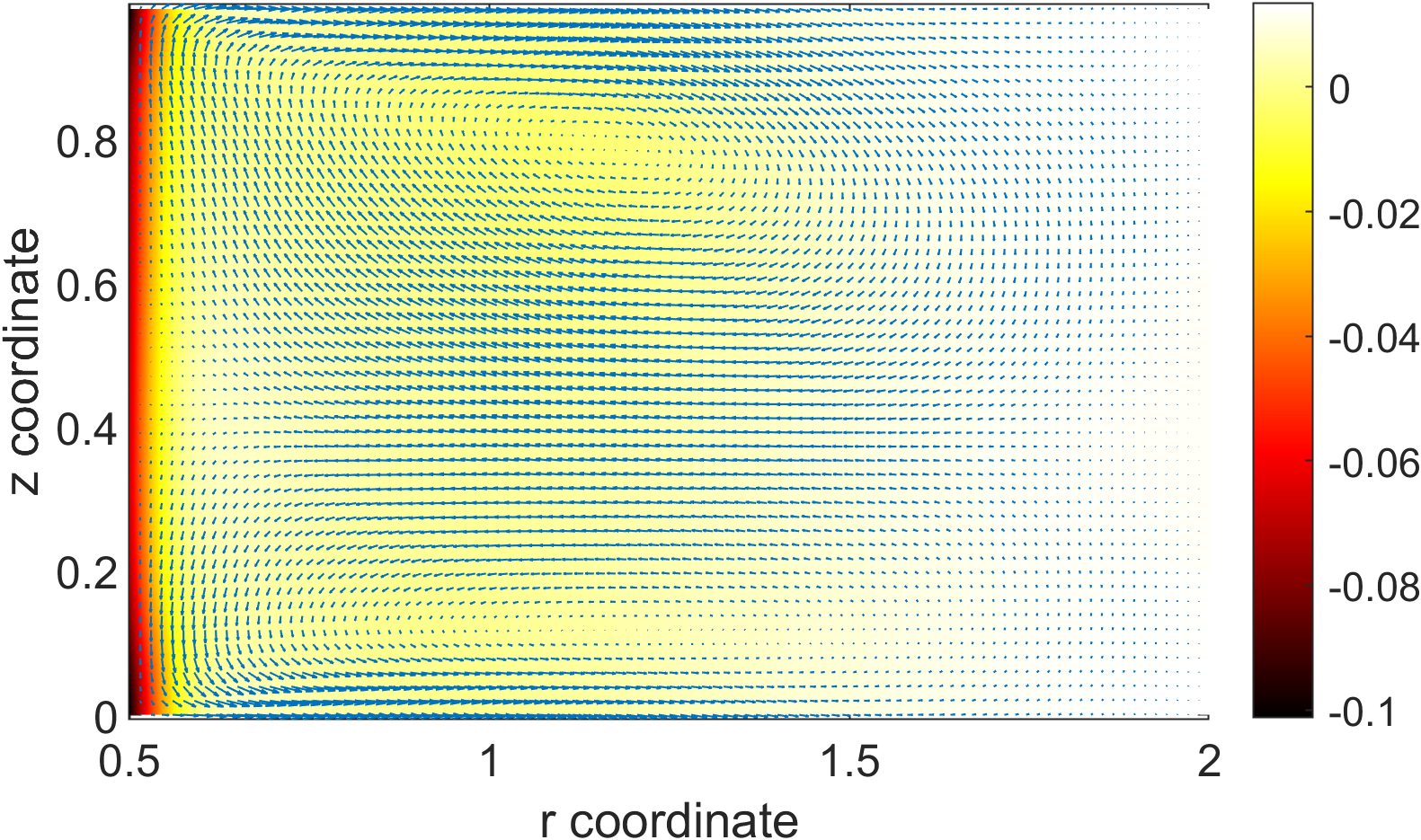
(d) Re = 300

Figure 20: Pressure plots in the plane along semi major axis of ellipse

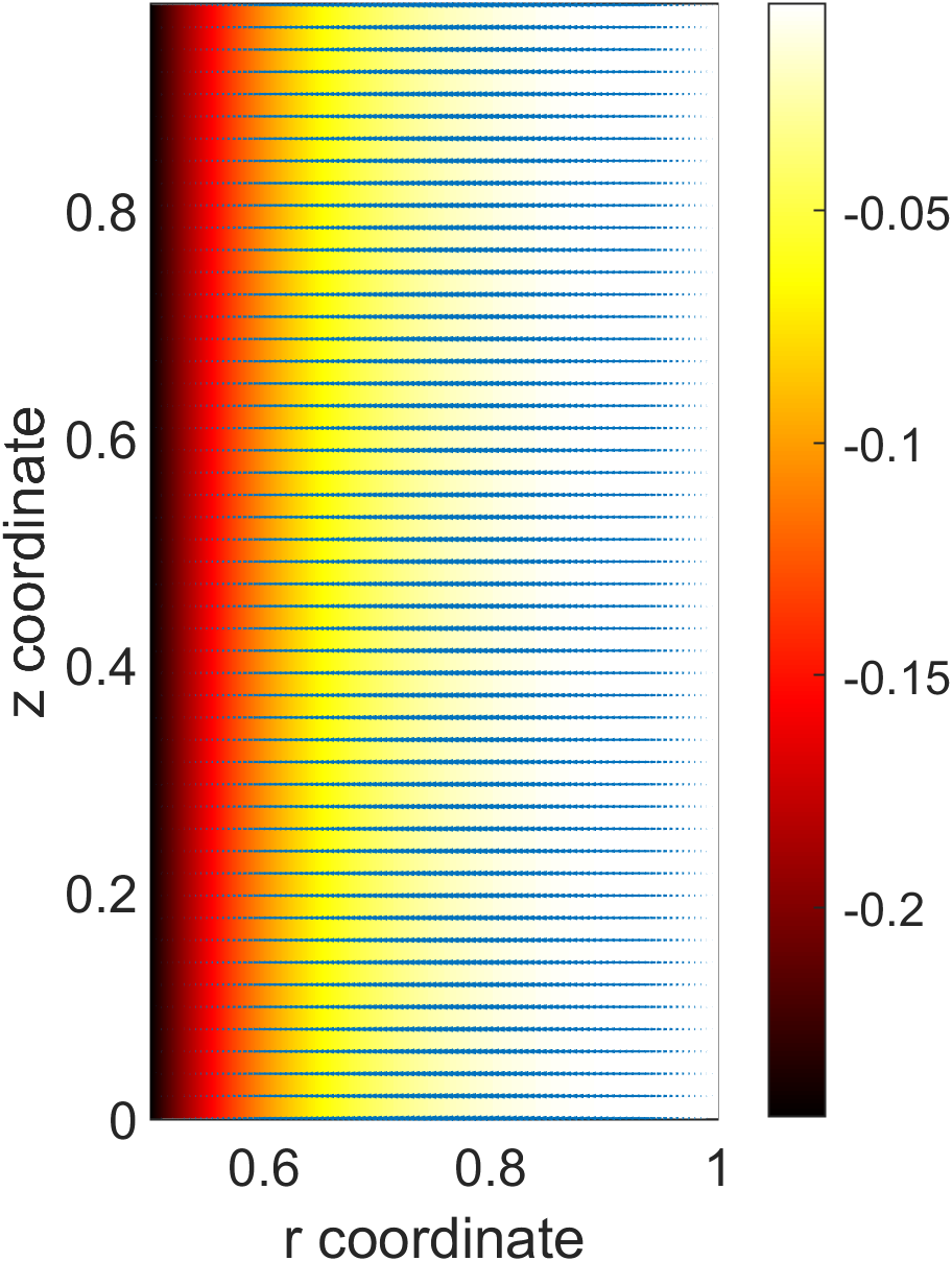
(a) Re = 70

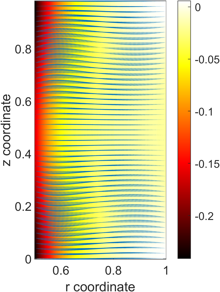
(b) Re = 75

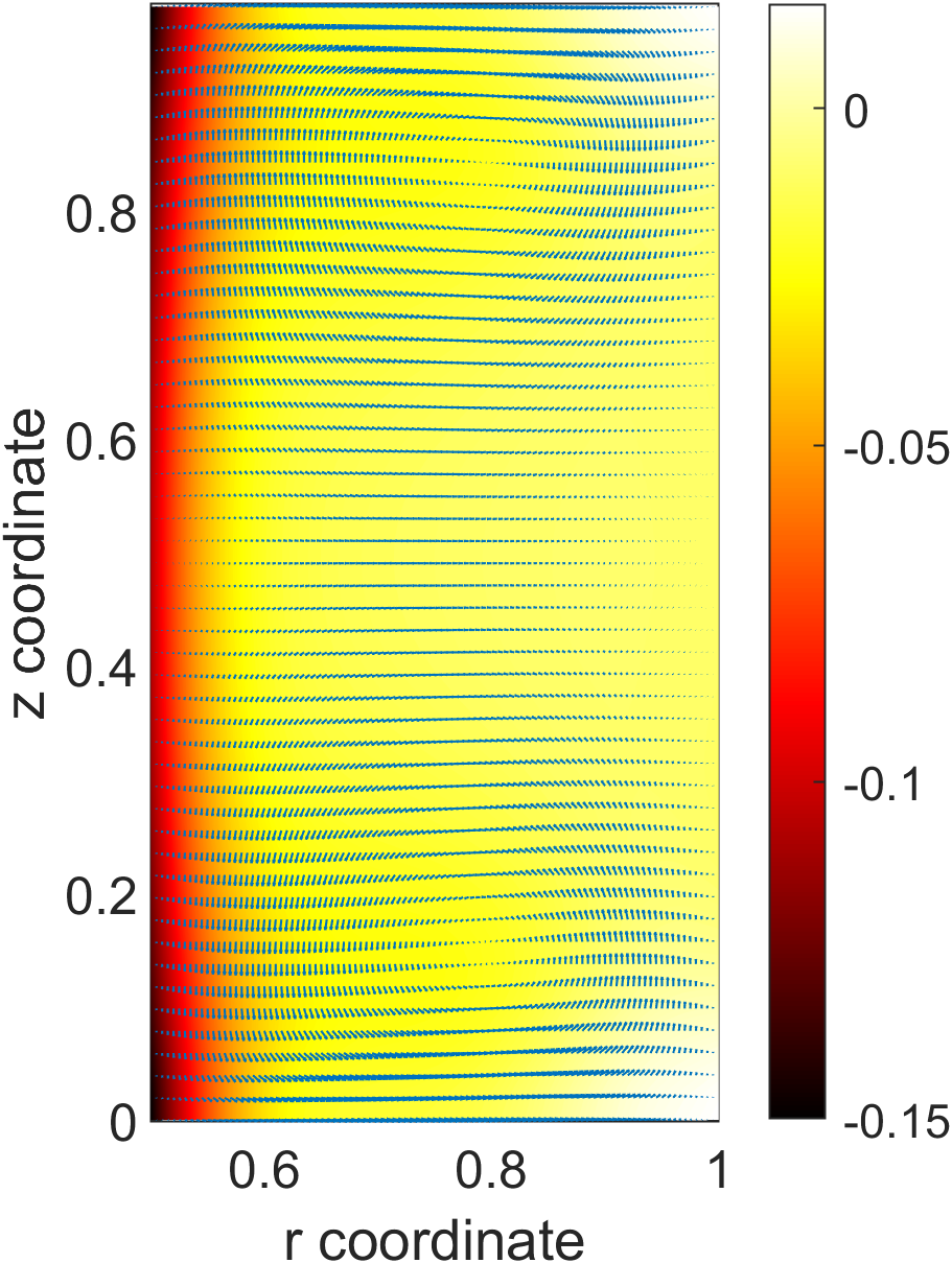
(c) Re = 200

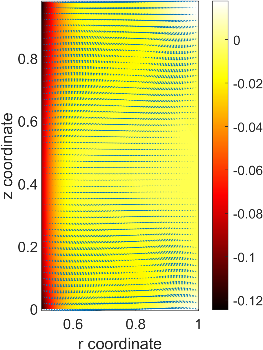
(d) Re = 300

Figure 21: Pressure plots in the plane along semi minor axis of ellipse

4.4.2 Isosurfaces of pressure

Figures 22 and 23 show the isosurfaces of the pressure in two views for pressure magnitude of $0.01$. The surfaces of the pressure show the distortions due to the Taylor cells. The bellow like shape of the isosurface indicate that there exists an alternating high pressure and low pressure regions along the axis. High pressure region are observed at the sections in between the Taylor cells and low pressure at the midsection of the Taylor cells. The formation of finger-like structures in the isosurfaces of pressure in fig. 22 can be seen to form as the flow approaches the minor axis of ellipse. This region being the shortest gap acts as a venturi to increase the speed of flow in between and as a result in the decrease of pressure. The tips of these finger-like structures being at an axial section between the two counter rotating Taylor cells, the pressure is observed to reduce below a value of 0.01.At $Re=300$ a slight deformation in the structure is observed, where the surface seems to be slightly inclined to the axis indicating formation of a spiral flow.

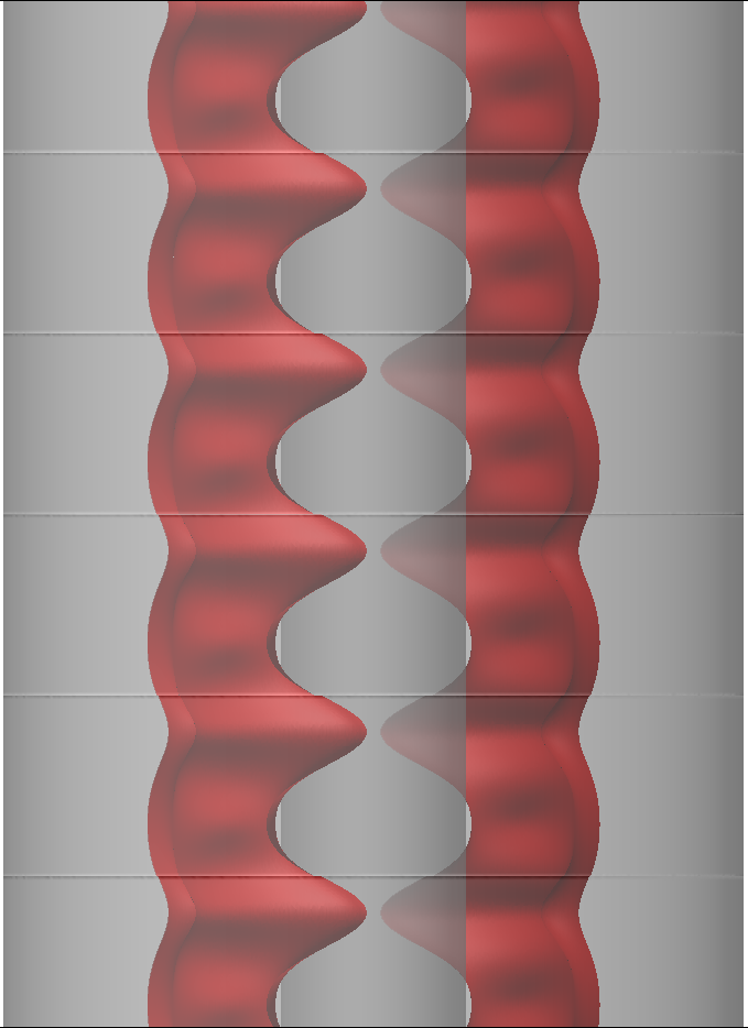
(a) Re = 75

(b) Re = 100

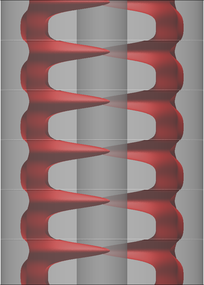
(c) Re = 200

(d) Re = 300

Figure 22: Isosurfaces of pressure for $p=0.01$, viewed from $x-z$ plane (view on the major axis section of ellipse)

(a) Re = 75

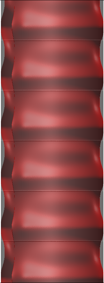
(b) Re = 100

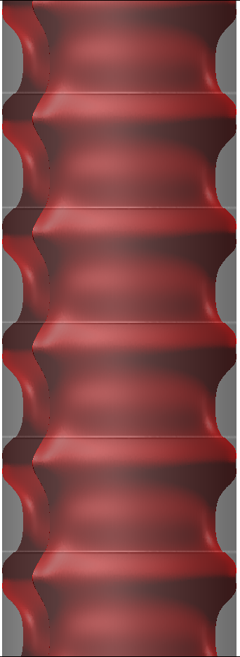
(c) Re = 200

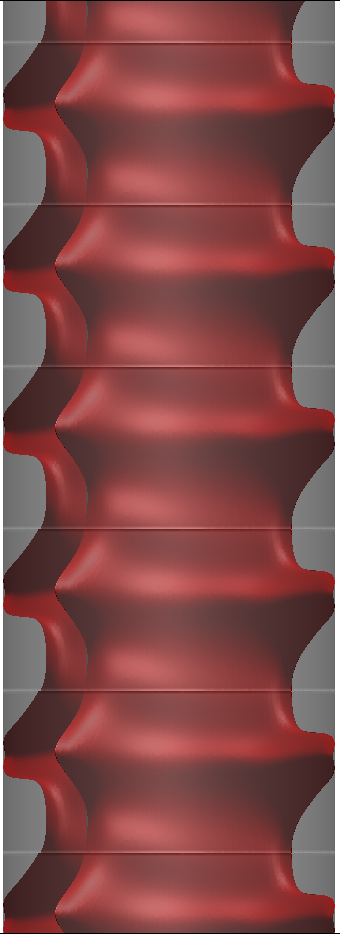
(d) Re = 300

Figure 23: Isosurfaces of pressure for $p=0.01$, viewed from $y-z$ plane (view on the minor axis section of ellipse)

4.5 Vorticity distributions

Vorticity, $\eta$, is defined as the curl of velocity vector ($\nabla\times\textbf{u}$) with components in $x,y,$ and $z$ directions. It measures the amount of rotation of a fluid element along the local axis. The magnitude of vorticity vector measures the strength of the local rotation of the fluid. In the following subsections, contours of vorticity magnitude in different planes and the isosurfaces of vorticity magnitude are presented.

4.5.1 Contours of vorticity magnitude in r-z planes

At subcritical $Re$, the vorticity is only due to motion in the $x-y$ plane. Since the cross-section is an ellipse, we see differences in distribution along major and minor axes. In figs. 24 and 25, we have plotted the contours of vorticity magnitude in two $r-z$ planes corresponding to major and minor axes. At subcritical $Re$ of $70$, the vorticity is quite small. However, at $Re=75$, due to the formation of the Taylor cells, the vorticity near the inner wall ($r=0.5$) increases due to the shear component $\frac{\partial w}{\partial r}$. This vorticity incresase as the cells strengthen with Reynolds number. Although the cells rotate in opposite direction, since we have plotted the magnitude, it is seen to be symmetric about $z=0.5$. At the top and bottom of the contours, we see ”fingers” of vorticity, which are a result of the flow turning at the corners of the Taylor cells. These increase with Reynolds number and at $Re=300$, we see some asymmetry probably due to the onset of spiral flow. We observe the same features in the minor gap, but the fingers of vorticity are stronger at the bottom for $Re=300$. This may be because the spiral vortices in the major gap are realigning to be more axisymmetric in the minor gap.

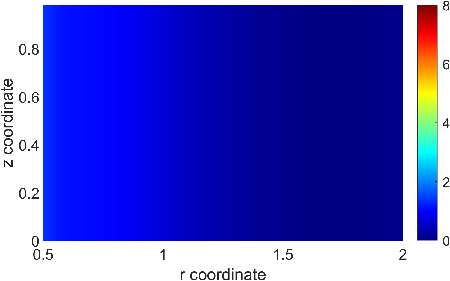
(a) Re = 70

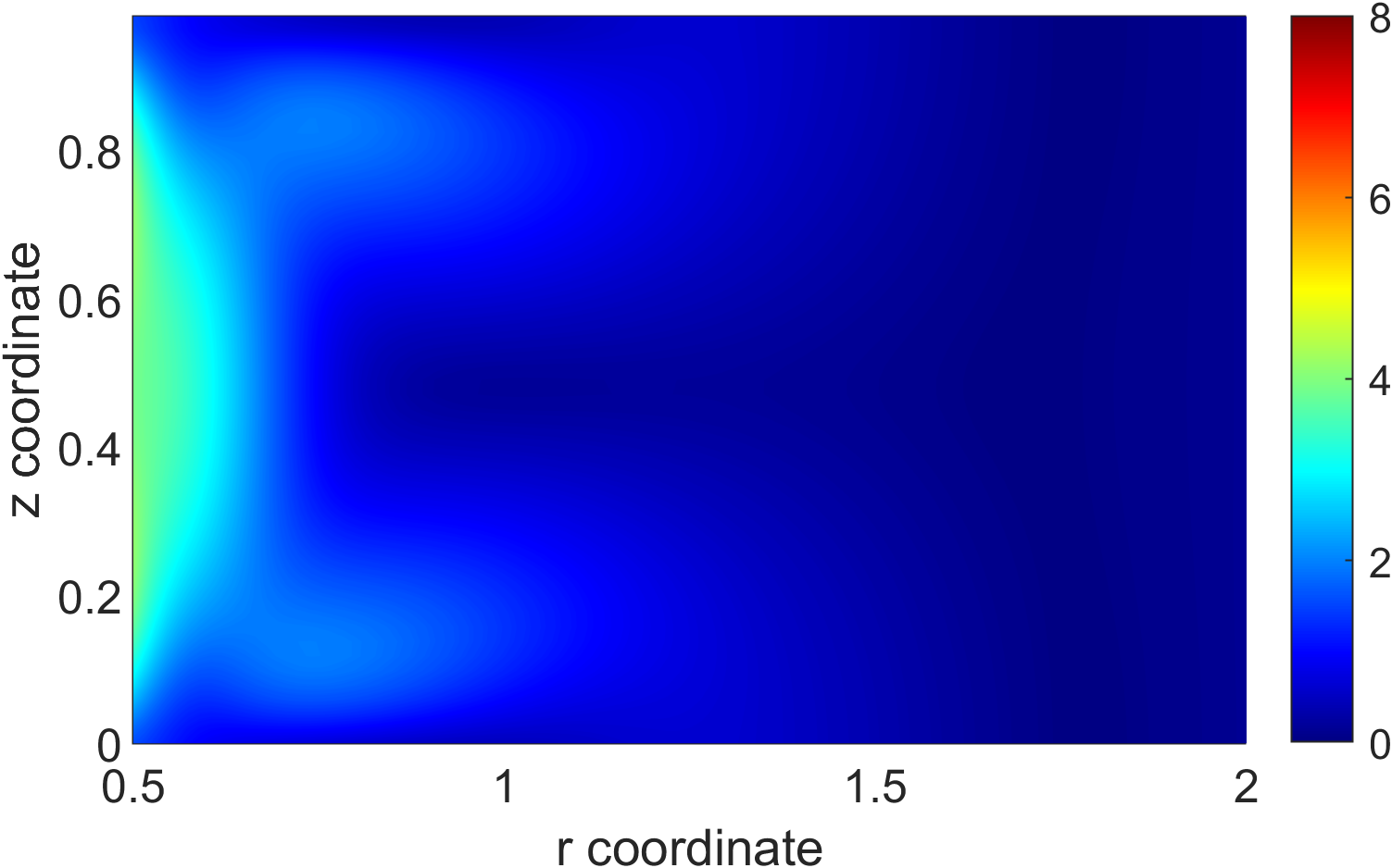
(b) Re = 75

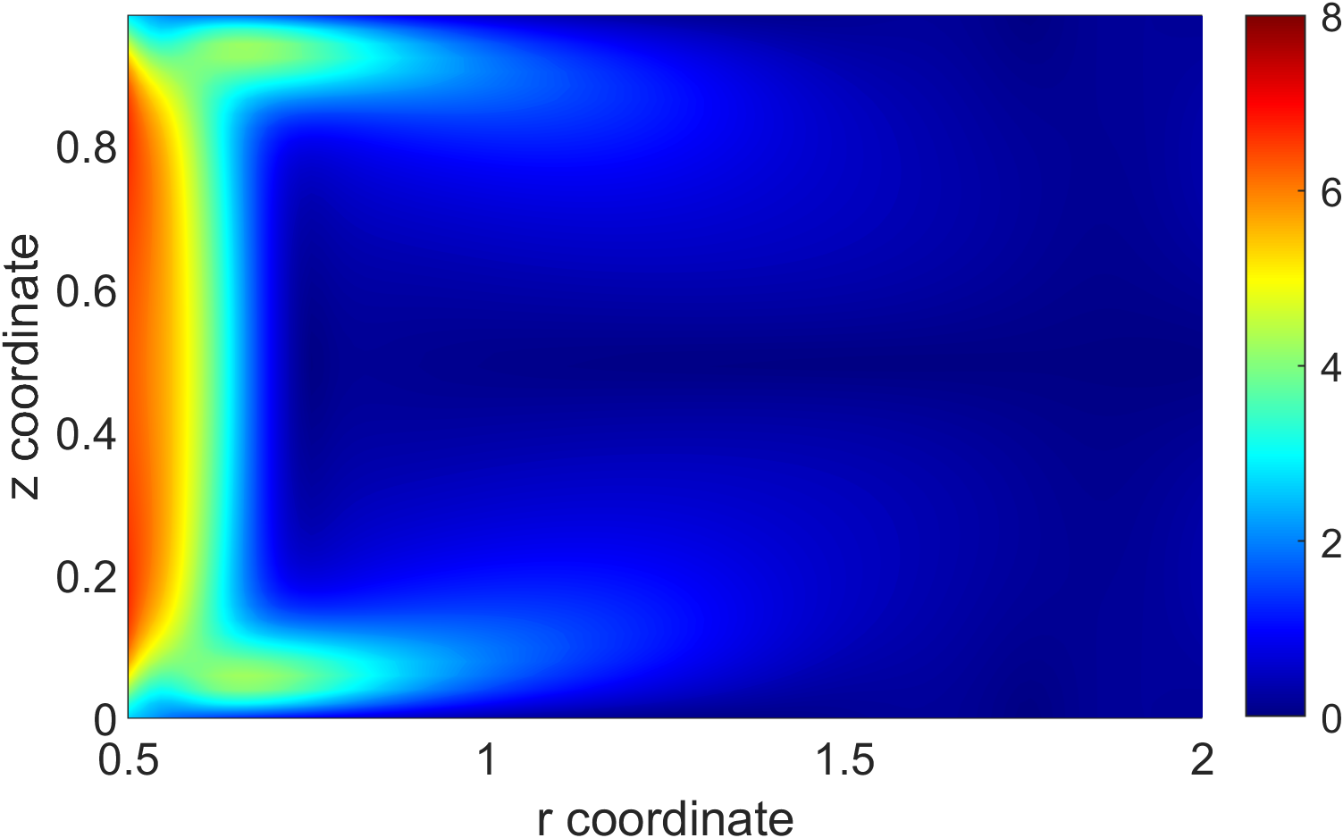
(c) Re = 200

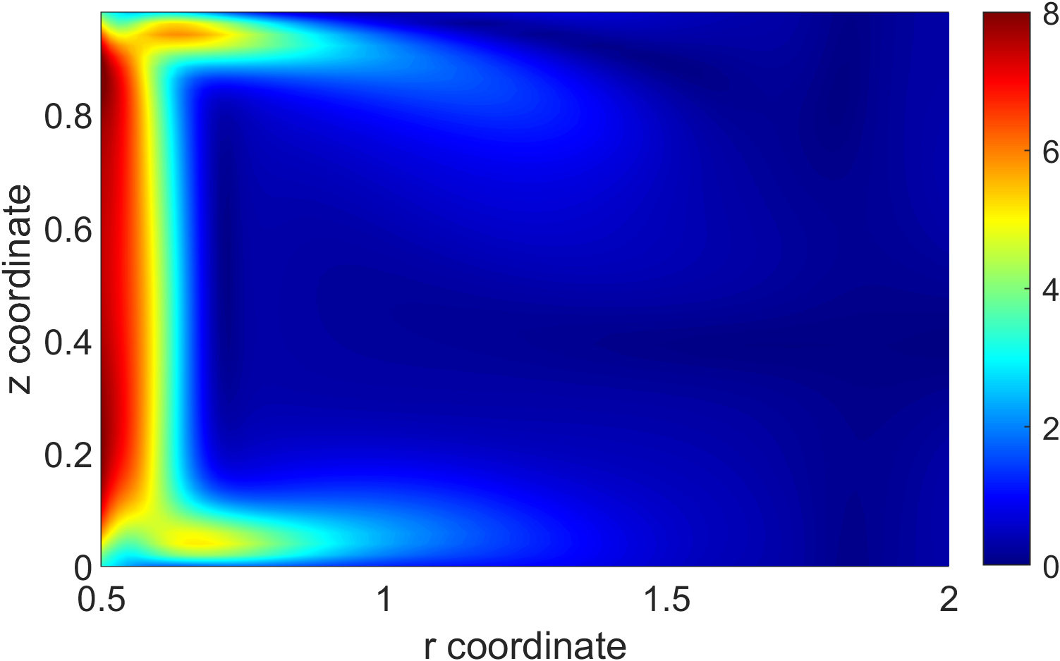
(d) Re = 300

Figure 24: Contours of vorticity magnitude in the plane along semi major axis of ellipse

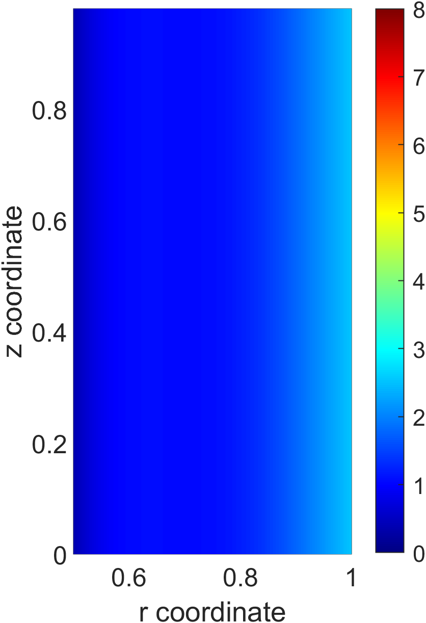
(a) Re = 70

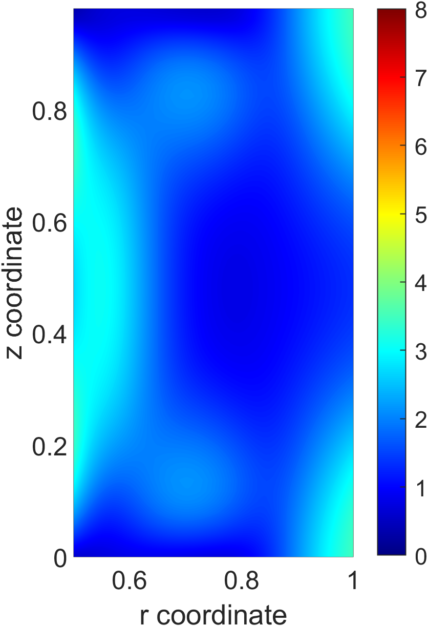
(b) Re = 75

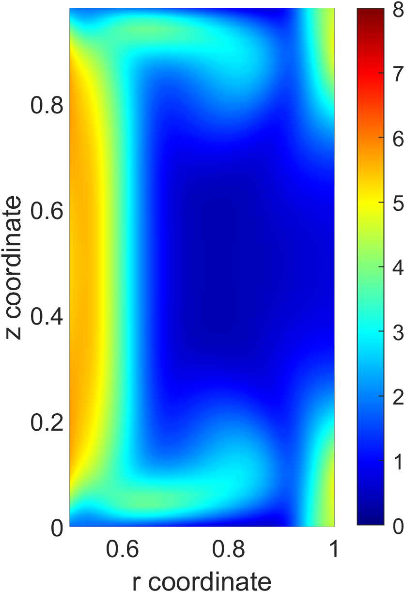
(c) Re = 200

(d) Re = 300

Figure 25: Contours of vorticity magnitude in the plane along semi minor axis of ellipse

4.5.2 Isosurfaces of vorticity magnitude

More visual information can be obtained from surfaces of iso-vorticity in the major and minor gap regions. We show surfaces of vorticity magnitude of $2.0$ non-dimensional units. It can be seen that vorticity is concentrated near the inner rotating cylinder and in the return flows from the inner and outer cylinder. The slight tilt at $Re=300$ is seen in the major gap with the vortices tilting upwards. The tilt of vorticity reinforce the same patterns seen for the pressure and axial velocity.

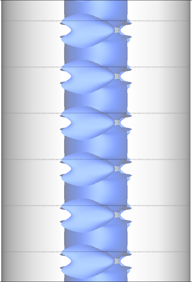
(a) Re = 75

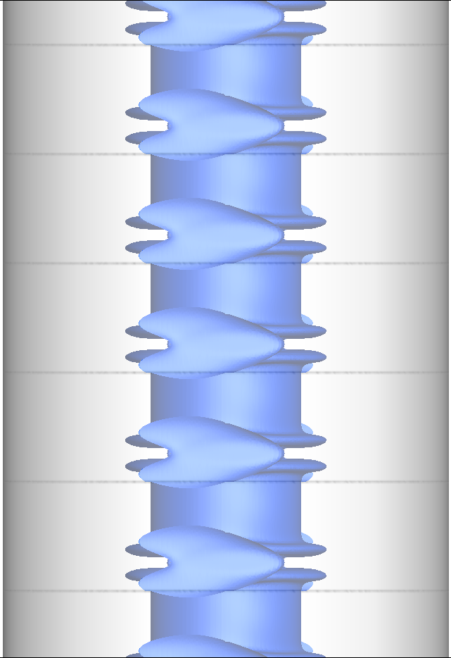
(b) Re = 100

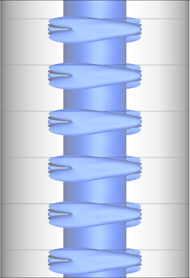
(c) Re = 200

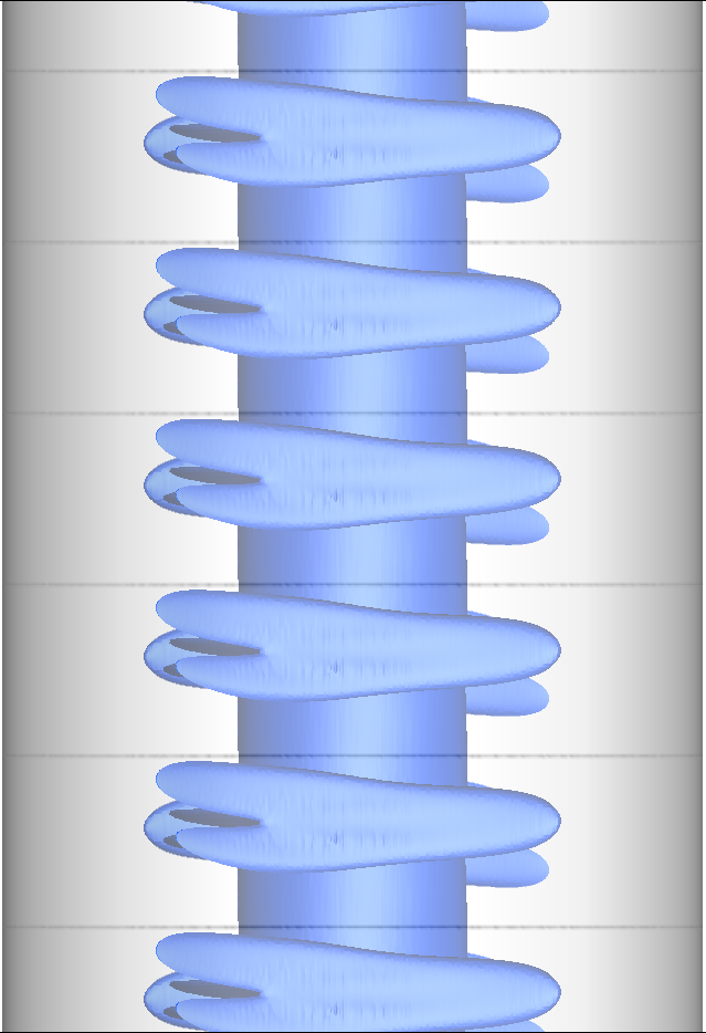
(d) Re = 300

Figure 26: Isosurfaces of vorticity magnitude for $\eta=2.0$, viewed from $x-z$ plane (view on the major axis section of ellipse)

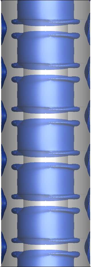
(a) Re = 75

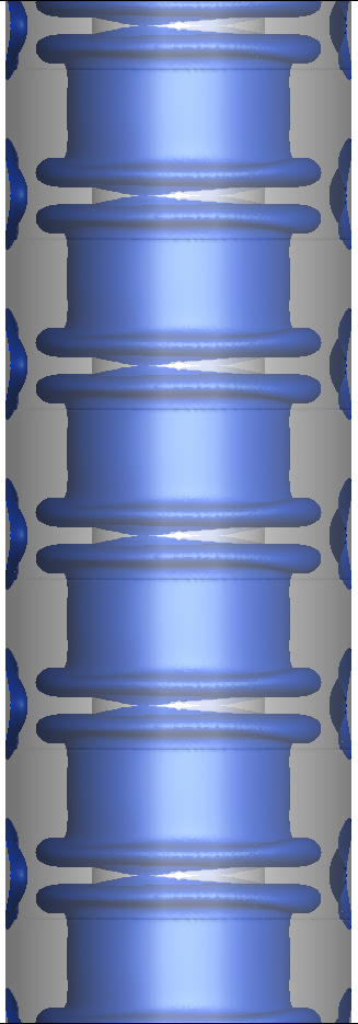
(b) Re = 100

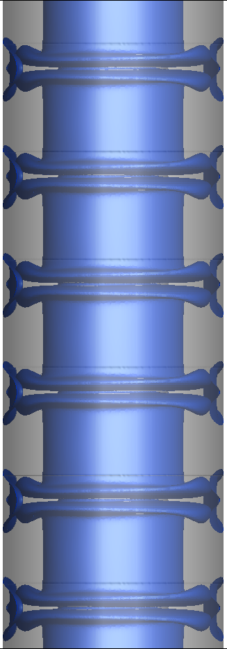
(c) Re = 200

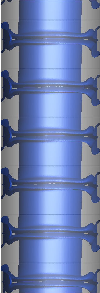
(d) Re = 300

Figure 27: Isosurfaces of vorticity magnitude for $\eta=2.0$, viewed from $y-z$ plane (view on the minor axis section of ellipse)

4.6 Q criterion

Q criterion is a mathematical tool used in fluid dynamics to identify regions prone to turbulence. A positive and high value of Q criterion, helps to visualise regions of high vorticity and shear, where vortex stretching is dominant. These regions are more likely to be turbulent compared to a negative Q criterion value indicating vortex compression. It is commonly used to visualise the location and extent of turbulent regions in a fluid flow. The value of Q is defined as the second invariant of the velocity gradient tensor given by:

$$Q=\frac{1}{2}(||\Omega||^{2}-||S||^{2})$$ (21)

where $S$ is the strain rate tensor given as $S=\frac{1}{2}\left[\left(\partial u_{i}/\partial x_{j}\right)+\left(\partial u_{j}/\partial x_{i}\right)\right]$ and $\Omega$ is the rotation rate or vorticity tensor given as $\Omega=\frac{1}{2}\left[\left(\partial u_{i}/\partial x_{j}\right)-\left(\partial u_{j}/\partial x_{i}\right)\right]$

4.6.1 Isosurfaces of Q criterion

The Q criteria surfaces in figs. 28 and 29 indicate the tendency of flow to become turbulent. The region where the flow is more prone to turbulence is the region between two counter rotating Taylor cells. At $Re=300$, where the wavy Taylor cells are formed, the Q surface is also tilted and wavy in nature. This actually indicates that the region between Taylor cells, where the axial velocity peaks, is where the flow tends to be turbulent before any other portion of the flow regime.

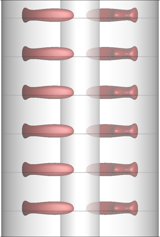
(a) Re = 75

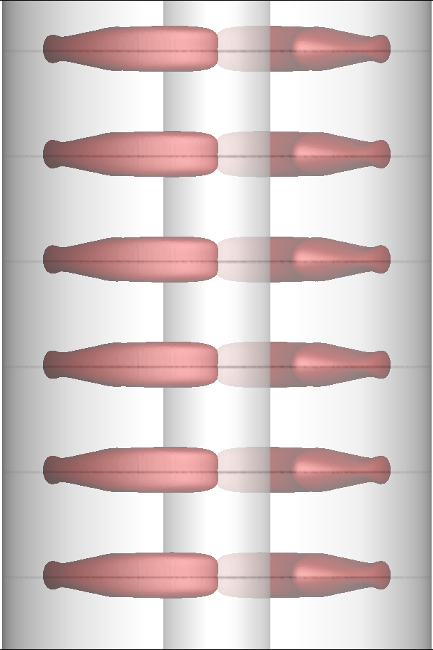
(b) Re = 100

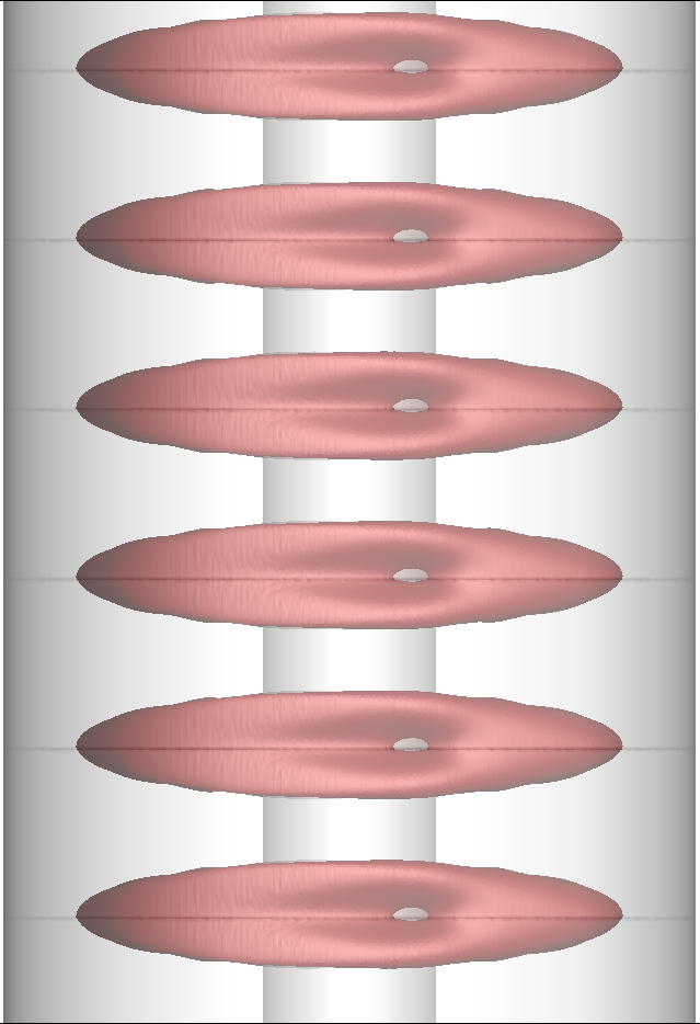
(c) Re = 200

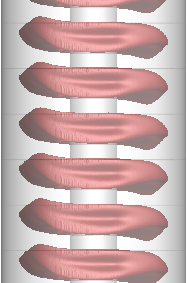
(d) Re = 300

Figure 28: Isosurfaces of $Q=1.0$, viewed from $x-z$ plane (view on the major axis section of ellipse)

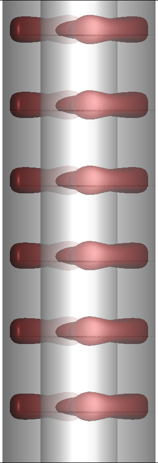
(a) Re = 75

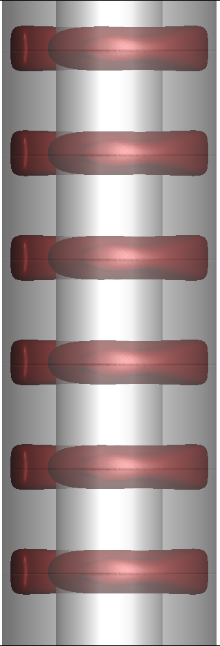
(b) Re = 100

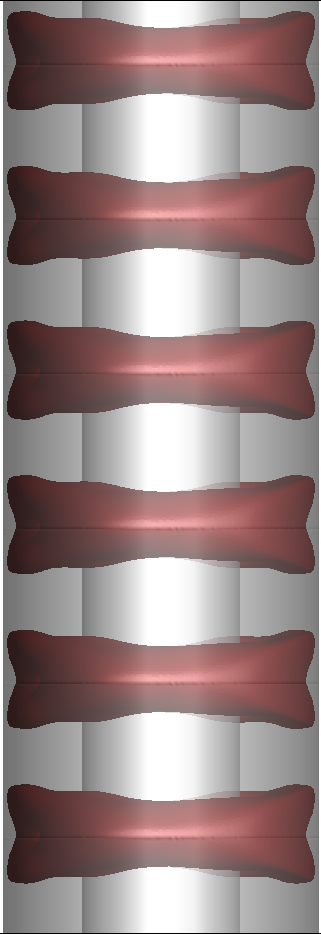
(c) Re = 200

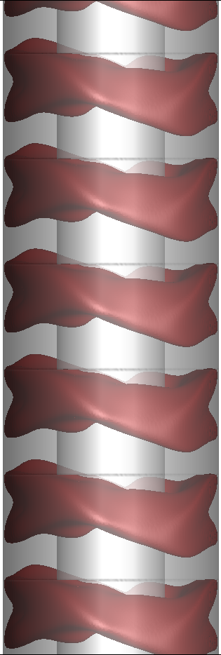
(d) Re = 300

Figure 29: Isosurfaces of $Q=1.0$, viewed from $y-z$ plane (view on the minor axis section of ellipse)

4.7 Temperature distributions

We finally present results of heat transfer from the inner wall. The inner wall is heated at a non-dimensional temperature of $1.0$ and the outer wall is maintained at $T=0$. The heat transfer rates in the form of the Nusselt number were earlier presented in fig. 5(b).

4.7.1 Contours of temperature in r-z planes

The temperature contours for supercritical Reynolds number show the effect of fluid motion in the Taylor cells. The hot fluid from the top and bottom circulations is carried from inner wall to the outer wall and returns the colder fluid from outer wall to the inner cylinder. This is seen to increase with Reynolds number as the strength of the circulation increases. The same pattern is seen in the minor gap plane. Similar to all the other field variables that we have discussed, the contours shown in figs. 30 and 31 has a symmetry about the plane $z=0.5$ for Reynolds number lesser than 300. The lose of symmetry that we see at the Reynolds number of 300 is due to the wavy nature of Taylor cells at this regime.

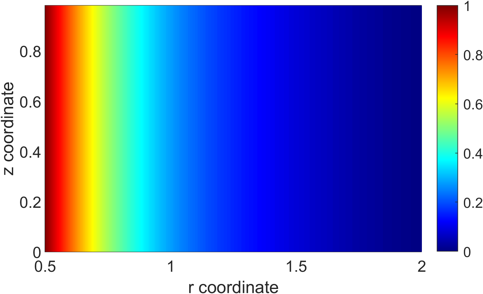
(a) Re = 70

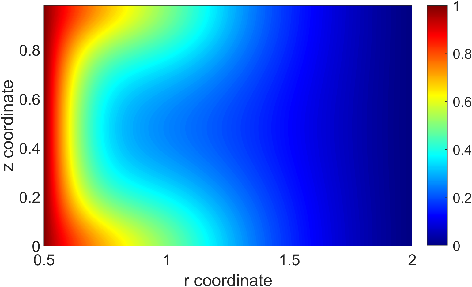
(b) Re = 75

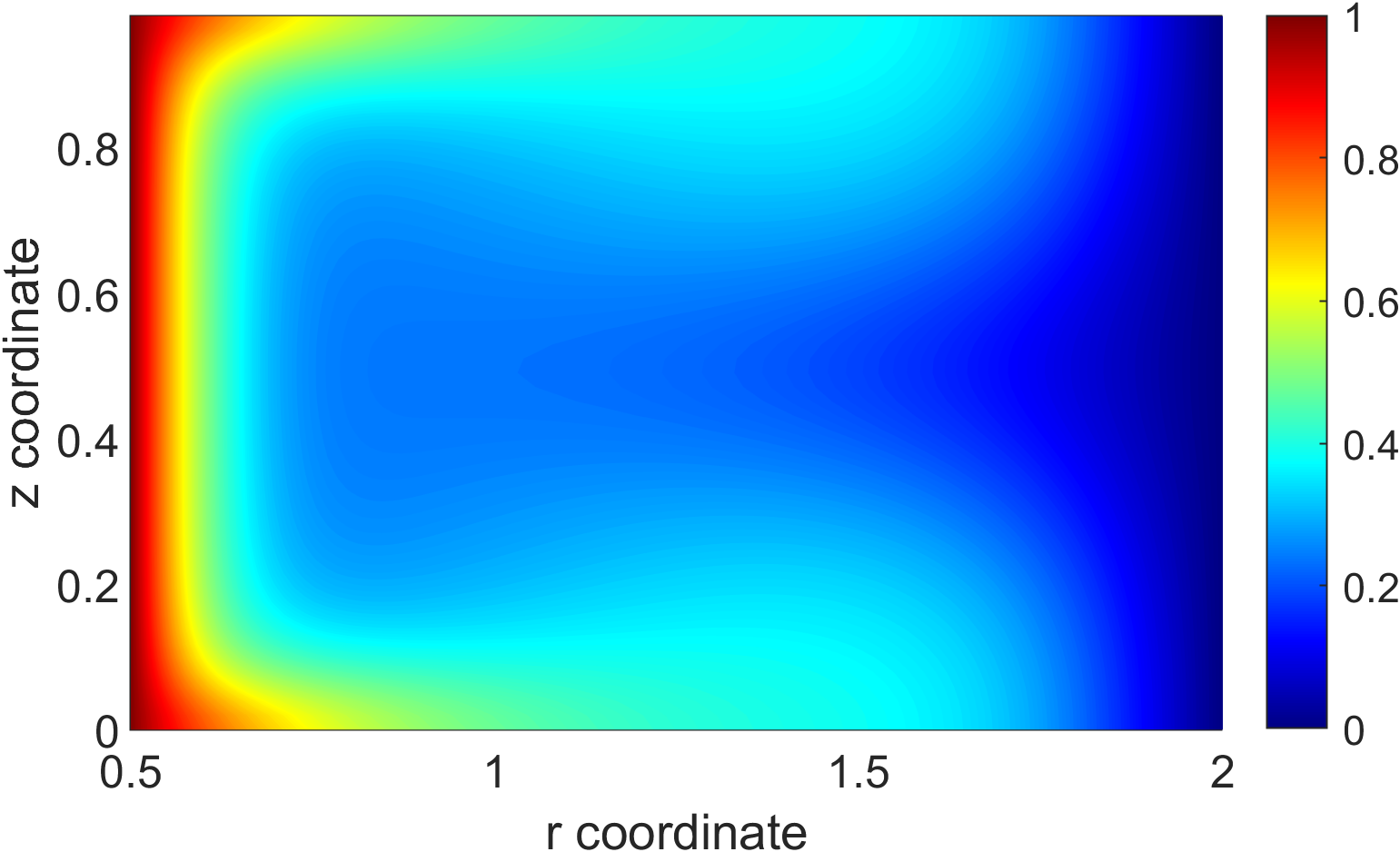
(c) Re = 200

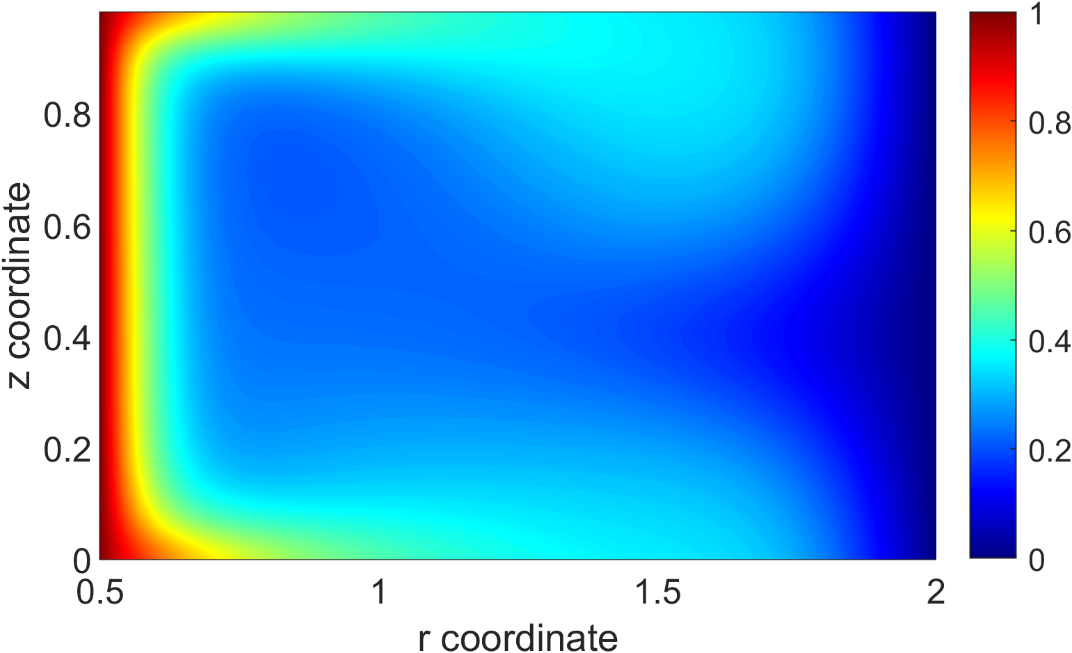
(d) Re = 300

Figure 30: Contours of temperature in the plane along semi major axis of ellipse

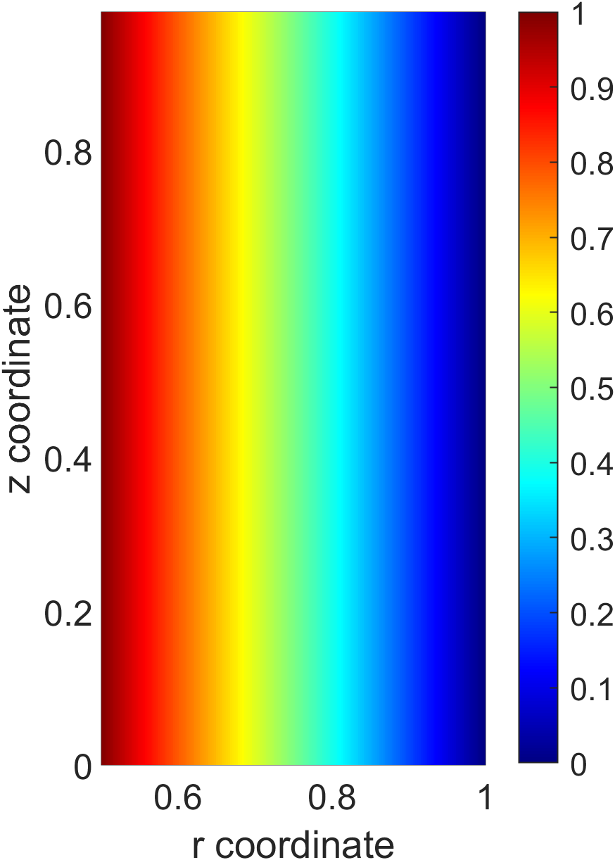
(a) Re = 70

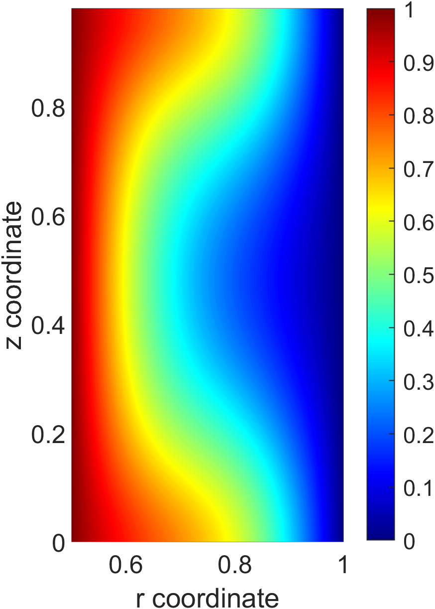
(b) Re = 75

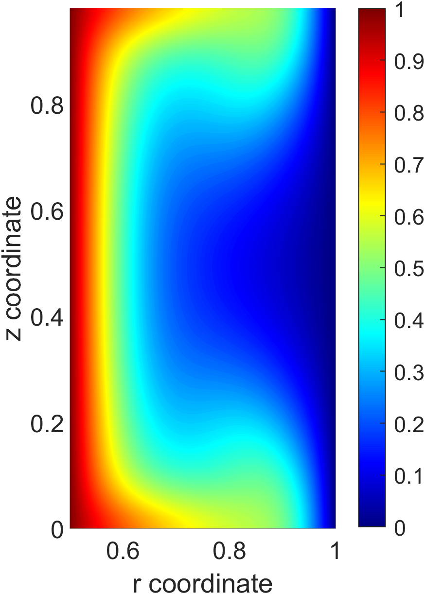
(c) Re = 200

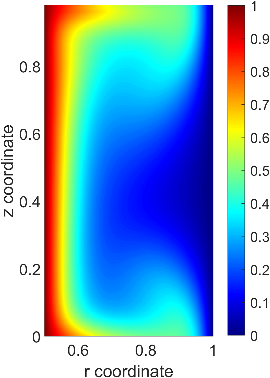
(d) Re = 300

Figure 31: Contours of temperature in the plane along semi minor axis of ellipse

4.7.2 Isosurfaces of temperature

Isosurfaces of temperature are in the form of bellows for supercritical cases with Reynolds number less than 300. Since temperature is solved as a scalar transport equation, it follows the fluid flow. i.e, the bulge on the bellows occur at the region between the Taylor cells where it meets the outer cylinder, since the flow is radially outward in this region. Similarly the trough of the bellow shape occurs at the section between the Taylor cells where the flow is radially inward meeting the inner cylinder. The surface for $Re=300$ has the slanted nature as the Taylor cells have a spiral nature.

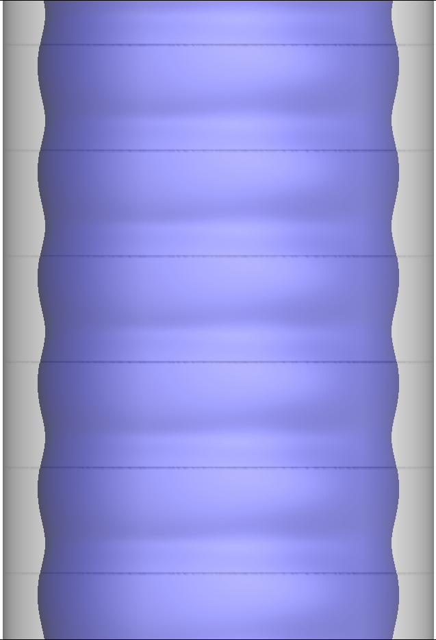
(a) Re = 75

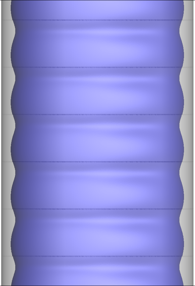
(b) Re = 100

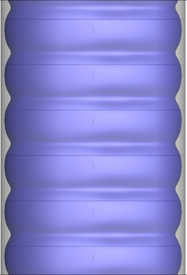
(c) Re = 200

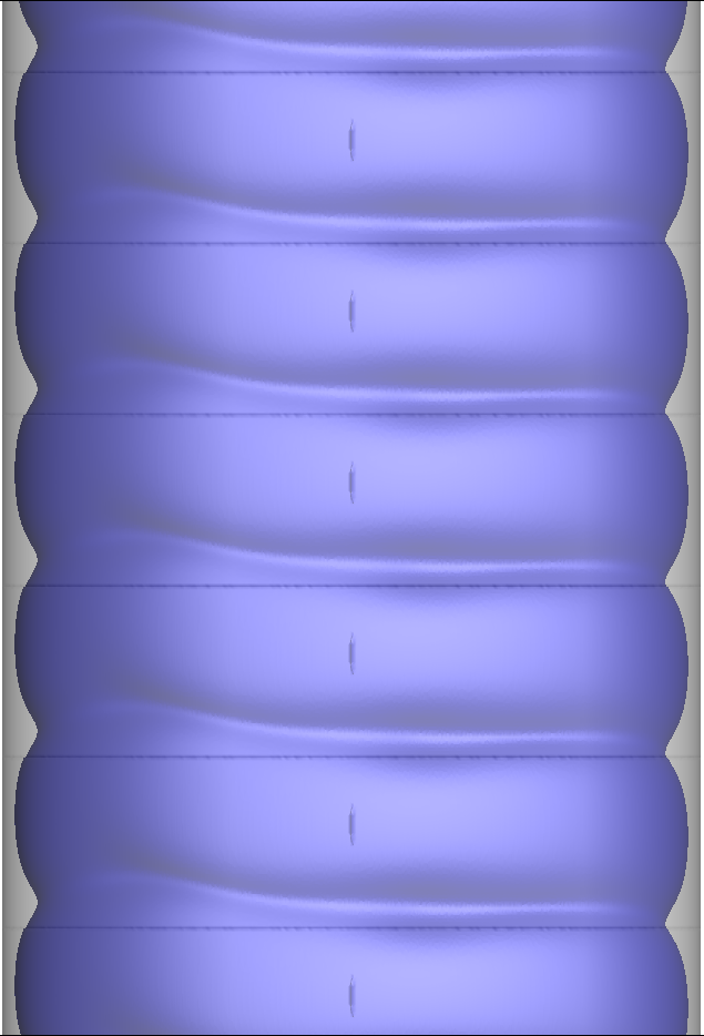
(d) Re = 300

Figure 32: Isosurfaces of temperature for $T=0.1$, viewed from $x-z$ plane (view on the major axis section of ellipse)

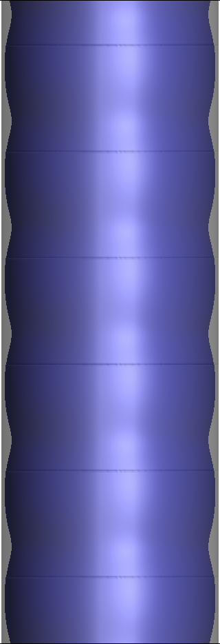
(a) Re = 75

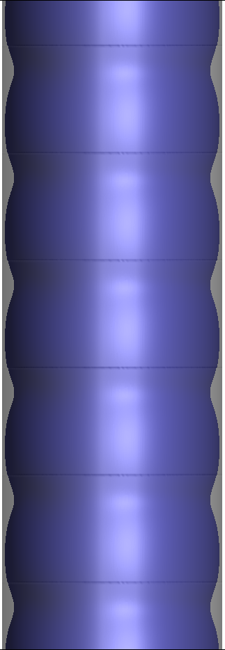
(b) Re = 100

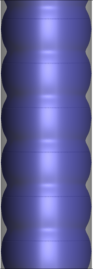
(c) Re = 200

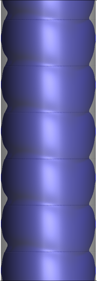
(d) Re = 300

Figure 33: Isosurfaces of temperature for $T=0.1$, viewed from $y-z$ plane (view on the minor axis section of ellipse)

5 Summary

In this paper, we have applied a novel Fourier-spectral meshless technique to study the development and characteristics of Taylor cells in an ellipse (aspect ratio of 2) with an inner circular cylinder rotating concentrically. The meshless technique solves the Navier-Stokes equations in Cartesian coordinates at scattered locations using stencils derived through Radial Basis Function interpolations. We have assumed periodicity in the axial direction, allowing a Fourier-spectral expansion along the axis of the cylinders. The Navier-Stokes equations are first converted to the Fourier space and the resulting equations for wave numbers are solved by the meshless method. The distributions of velocity, pressure, temperature, and vorticity are presented for subcritical and supercritical regions. The torque on the inner cylinder and the critical Reynolds number for formation of the Taylor cells are found to be nearly the same as the concentric circular cylinder results in literature. However, the structure of the Taylor cells is different in the ellipse because of the compression and expansion of the Taylor vortices as they pass between the major and minor gaps. At low Reynolds numbers, the Taylor cells are concentrically structured forming a square shape in the minor gaps and a rectangular shape in the major gaps respectively, as a result of the stretch and squeeze between the gaps. However, these structured cells slowly deform when the Reynolds number reaches 300, indicating a transition to a wavy pattern. We present isosurfaces of the axial velocity, pressure, vorticity, and temperature which indicate the shape of the Taylor cells. These surfaces of iso-values appear consistent with the squeezing and expansions of the cells between the gaps.

Data Availability

The data that support the findings of this study are available from the corresponding author upon reasonable request.

Author Declarations

The authors have no conflicts to disclose.

References

- Mallock [1889] A. Mallock, IV. Determination of the viscosity of water, Proceedings of the Royal Society of London 45 (1889) 126–132.
- Mallock [1896] A. Mallock, III. Experiments on fluid viscosity, Philosophical Transactions of the Royal Society of London. Series A, Containing Papers of a Mathematical or Physical Character (1896) 41–56.
- Couette [1890] M. Couette, Distinction de deux régimes dans le mouvement des fluides, Journal de Physique Théorique et Appliquée 9 (1890) 414–424.
- Taylor [1923] G. I. Taylor, VIII. Stability of a viscous liquid contained between two rotating cylinders, Philosophical Transactions of the Royal Society of London. Series A, Containing Papers of a Mathematical or Physical Character 223 (1923) 289–343.
- Coles [1965] D. Coles, Transition in circular Couette flow, Journal of Fluid Mechanics 21 (1965) 385–425. doi:10.1017/S0022112065000241.
- Andereck et al. [1986] C. D. Andereck, S. S. Liu, H. L. Swinney, Flow regimes in a circular Couette system with independently rotating cylinders, Journal of Fluid Mechanics 164 (1986) 155–183. doi:10.1017/S0022112086002513.
- Fenstermacher et al. [1979] P. R. Fenstermacher, H. L. Swinney, J. P. Gollub, Dynamical instabilities and the transition to chaotic Taylor vortex flow, Journal of Fluid Mechanics 94 (1979) 103–128. doi:10.1017/S0022112079000963.
- Snyder [1968] H. Snyder, Stability of rotating Couette flow. I. Asymmetric waveforms, The Physics of Fluids 11 (1968) 728–734.
- Snyder [1969] H. Snyder, Change in wave-form and mean flow associated with wavelength variations in rotating Couette flow. Part 1, Journal of Fluid Mechanics 35 (1969) 337–352.
- DiPrima and Stuart [1972a] R. DiPrima, J. Stuart, Flow between eccentric rotating cylinders (1972a).
- DiPrima and Stuart [1972b] R. DiPrima, J. Stuart, Non-local effects in the stability of flow between eccentric rotating cylinders, Journal of Fluid Mechanics 54 (1972b) 393–415.
- DiPrima and Stuart [1975] R. DiPrima, J. Stuart, The nonlinear calculation of taylor-vortex flow between eccentric rotating cylinders, Journal of Fluid Mechanics 67 (1975) 85–111.
- DiPrima and Eagles [1977] R. DiPrima, P. Eagles, Amplification rates and torques for Taylor-vortex flows between rotating cylinders, The Physics of Fluids 20 (1977) 171–175.
- Stuart and Di Prima [1980] J. T. Stuart, R. Di Prima, On the mathematics of Taylor-vortex flows in cylinders of finite length, Proceedings of the Royal Society of London. A. Mathematical and Physical Sciences 372 (1980) 357–365.
- Smith and Townsend [1982] G. Smith, A. Townsend, Turbulent Couette flow between concentric cylinders at large Taylor numbers, Journal of Fluid Mechanics 123 (1982) 187–217.
- Davey et al. [1968] A. Davey, R. Di Prima, J. Stuart, On the instability of Taylor vortices, Journal of Fluid Mechanics 31 (1968) 17–52.
- Lorenzen and Mullin [1985] A. Lorenzen, T. Mullin, Anomalous modes and finite-length effects in Taylor-Couette flow, Physical Review A 31 (1985) 3463.
- Mullin et al. [2002] T. Mullin, Y. Toya, S. Tavener, Symmetry breaking and multiplicity of states in small aspect ratio Taylor-Couette flow, Physics of Fluids 14 (2002) 2778–2787.
- Czarny et al. [2002] O. Czarny, E. Serre, P. Bontoux, R. M. Lueptow, Spiral and wavy vortex flows in short counter-rotating Taylor-Couette cells, Theoretical and computational fluid dynamics 16 (2002) 5–15.
- Schulz et al. [2003] A. Schulz, G. Pfister, S. Tavener, The effect of outer cylinder rotation on Taylor-Couette flow at small aspect ratio, Physics of Fluids 15 (2003) 417–425.
- Bilson and Bremhorst [2007] M. Bilson, K. Bremhorst, Direct numerical simulation of turbulent Taylor-Couette flow, Journal of Fluid Mechanics 579 (2007) 227–270.
- Pirro and Quadrio [2008] D. Pirro, M. Quadrio, Direct numerical simulation of turbulent Taylor-Couette flow, European Journal of Mechanics-B/Fluids 27 (2008) 552–566.
- Brauckmann and Eckhardt [2013] H. J. Brauckmann, B. Eckhardt, Direct numerical simulations of local and global torque in Taylor-Couette flow up to Re= 30000, Journal of Fluid Mechanics 718 (2013) 398–427.
- Dong [2007] S. Dong, Direct numerical simulation of turbulent Taylor-Couette flow, Journal of Fluid Mechanics 587 (2007) 373–393.
- Ostilla et al. [2013] R. Ostilla, R. J. Stevens, S. Grossmann, R. Verzicco, D. Lohse, Optimal Taylor-Couette flow: direct numerical simulations, Journal of fluid mechanics 719 (2013) 14–46.
- Wereley and Lueptow [1998] S. T. Wereley, R. M. Lueptow, Spatio-temporal character of non-wavy and wavy Taylor-Couette flow, Journal of Fluid Mechanics 364 (1998) 59–80.
- Huisman et al. [2012] S. G. Huisman, D. P. van Gils, S. Grossmann, C. Sun, D. Lohse, Ultimate turbulent Taylor-Couette flow, Physical review letters 108 (2012) 024501.
- Wereley and Lueptow [1999] S. T. Wereley, R. M. Lueptow, Inertial particle motion in a Taylor Couette rotating filter, Physics of fluids 11 (1999) 325–333.
- Wang et al. [2005] L. Wang, R. D. Vigil, R. O. Fox, CFD simulation of shear-induced aggregation and breakage in turbulent Taylor-Couette flow, Journal of colloid and interface science 285 (2005) 167–178.
- Majji and Morris [2018] M. V. Majji, J. F. Morris, Inertial migration of particles in Taylor-Couette flows, Physics of Fluids 30 (2018) 033303.
- Dash et al. [2020] A. Dash, A. Anantharaman, C. Poelma, Particle-laden Taylor-Couette flows: higher-order transitions and evidence for azimuthally localized wavy vortices, Journal of Fluid Mechanics 903 (2020).
- Holeschovsky and Cooney [1991] U. B. Holeschovsky, C. L. Cooney, Quantitative description of ultrafiltration in a rotating filtration device, AIChE Journal 37 (1991) 1219–1226.
- Lee and Lueptow [2001] S. Lee, R. M. Lueptow, Rotating reverse osmosis system based on Taylor-Couette flow, in: 12th International Couette-Taylor Workshop, 2001, pp. 6–8.
- Serre et al. [2008] E. Serre, M. A. Sprague, R. M. Lueptow, Stability of Taylor-Couette flow in a finite-length cavity with radial throughflow, Physics of Fluids 20 (2008) 034106.
- Tilton et al. [2010] N. Tilton, D. Martinand, E. Serre, R. M. Lueptow, Pressure-driven radial flow in a Taylor-Couette cell, Journal of fluid mechanics 660 (2010) 527–537.
- Tu et al. [2018] Q. Tu, T. Li, A. Deng, K. Zhu, Y. Liu, S. Li, A scale-up nanoporous membrane centrifuge for reverse osmosis desalination without fouling, Technology 6 (2018) 36–48.
- Cohen and Marom [1983] S. Cohen, D. M. Marom, Experimental and theoretical study of a rotating annular flow reactor, The Chemical Engineering Journal 27 (1983) 87–97.
- Poncet et al. [2011] S. Poncet, S. Haddadi, S. Viazzo, Numerical modeling of fluid flow and heat transfer in a narrow Taylor-Couette-Poiseuille system, International Journal of Heat and Fluid Flow 32 (2011) 128–144.
- Campero and Vigil [1999] R. J. Campero, R. D. Vigil, Flow patterns in liquid- liquid Taylor-Couette-Poiseuille flow, Industrial & engineering chemistry research 38 (1999) 1094–1098.
- Wereley and Lueptow [1999] S. T. Wereley, R. M. Lueptow, Velocity field for Taylor-Couette flow with an axial flow, Physics of Fluids 11 (1999) 3637–3649.
- Ball and Farouk [1988] K. Ball, B. Farouk, Bifurcation phenomena in Taylor-Couette flow with buoyancy effects, Journal of Fluid Mechanics 197 (1988) 479–501.
- Teng et al. [2015] H. Teng, N. Liu, X. Lu, B. Khomami, Direct numerical simulation of Taylor-Couette flow subjected to a radial temperature gradient, Physics of Fluids 27 (2015) 125101.
- Guillerm et al. [2015] R. Guillerm, C. Kang, C. Savaro, V. Lepiller, A. Prigent, K.-S. Yang, I. Mutabazi, Flow regimes in a vertical Taylor-Couette system with a radial thermal gradient, Physics of Fluids 27 (2015) 094101.
- Leng et al. [2021] X.-Y. Leng, D. Krasnov, B.-W. Li, J.-Q. Zhong, Flow structures and heat transport in Taylor-Couette systems with axial temperature gradient, Journal of Fluid Mechanics 920 (2021).
- Khawar et al. [2022] O. Khawar, M. Baig, S. Sanghi, Counter-rotating Taylor-Couette flows with radial temperature gradient, International Journal of Heat and Fluid Flow 95 (2022) 108980.
- Eagles et al. [1978] P. Eagles, J. Stuart, R. DiPrima, The effects of eccentricity on torque and load in Taylor-vortex flow, Journal of Fluid Mechanics 87 (1978) 209–231.
- Oikawa et al. [1989] M. Oikawa, T. Karasudani, M. Funakoshi, Stability of flow between eccentric rotating cylinders, Journal of the Physical Society of Japan 58 (1989) 2355–2364. URL: https://doi.org/10.1143/JPSJ.58.2355. doi:10.1143/JPSJ.58.2355. arXiv:https://doi.org/10.1143/JPSJ.58.2355.
- Shu et al. [2004] C. Shu, L. Wang, Y. Chew, N. Zhao, Numerical study of eccentric Couette-Taylor flows and effect of eccentricity on flow patterns, Theoretical and Computational Fluid Dynamics 18 (2004) 43–59.
- Krueger et al. [1966] E. Krueger, A. Gross, R. Di Prima, On the relative importance of Taylor-vortex and non-axisymmetric modes in flow between rotating cylinders, Journal of Fluid Mechanics 24 (1966) 521–538.
- Rui-Xiu et al. [1992] D. Rui-Xiu, Q. Dong, A. Szeri, Flow between eccentric rotating cylinders: Bifurcation and stability, International Journal of Engineering Science 30 (1992) 1323–1340. URL: https://www.sciencedirect.com/science/article/pii/0020722592901446. doi:https://doi.org/10.1016/0020-7225(92)90144-6.
- Leclercq et al. [2013] C. Leclercq, B. Pier, J. F. Scott, Temporal stability of eccentric Taylor-Couette-Poiseuille flow, Journal of fluid mechanics 733 (2013) 68–99.
- Leclercq et al. [2014] C. Leclercq, B. Pier, J. F. Scott, Absolute instabilities in eccentric Taylor-Couette-Poiseuille flow, Journal of fluid mechanics 741 (2014) 543–566.
- Sprague et al. [2008] M. Sprague, P. Weidman, S. Macumber, P. Fischer, Tailored Taylor vortices, Physics of fluids 20 (2008) 014102.
- Sprague and Weidman [2009] M. A. Sprague, P. D. Weidman, Continuously tailored Taylor vortices, Physics of fluids 21 (2009) 114106.
- Wimmer [1976] M. Wimmer, Experiments on a viscous fluid flow between concentric rotating spheres, Journal of Fluid Mechanics 78 (1976) 317–335.
- Nakabayashi and Tsuchida [1988a] K. Nakabayashi, Y. Tsuchida, Modulated and unmodulated travelling azimuthal waves on the toroidal vortices in a spherical Couette system, Journal of Fluid Mechanics 195 (1988a) 495–522.
- Nakabayashi and Tsuchida [1988b] K. Nakabayashi, Y. Tsuchida, Spectral study of the laminar—turbulent transition in spherical Couette flow, Journal of Fluid Mechanics 194 (1988b) 101–132.
- Wimmer [1995] M. Wimmer, An experimental investigation of Taylor vortex flow between conical cylinders, Journal of Fluid Mechanics 292 (1995) 205–227.
- Denne and Wimmer [1999] B. Denne, M. Wimmer, Travelling Taylor vortices in closed systems, Acta mechanica 133 (1999) 69–85.
- Soos et al. [2007] M. Soos, H. Wu, M. Morbidelli, Taylor-Couette unit with a lobed inner cylinder cross section, AIChE journal 53 (2007) 1109–1120.
- Snyder [1968] H. Snyder, Experiments on rotating flows between noncircular cylinders, The Physics of Fluids 11 (1968) 1606–1611.
- Mullin and Lorenzen [1985] T. Mullin, A. Lorenzen, Bifurcation phenomena in flows between a rotating circular cylinder and a stationary square outer cylinder, Journal of Fluid Mechanics 157 (1985) 289–303.
- Benjamin and Mullin [1981] T. Benjamin, T. Mullin, Anomalous modes in Taylor-Couette flow, Proc. R. Soc. A (London) 377 (1981) 221–249.
- Greidanus et al. [2015] A. Greidanus, R. Delfos, S. Tokgoz, J. Westerweel, Turbulent Taylor-Couette flow over riblets: drag reduction and the effect of bulk fluid rotation, Experiments in Fluids 56 (2015) 1–13.
- Razzak et al. [2020] M. A. Razzak, K. B. Cheong, K. B. Lua, Numerical study of Taylor-Couette flow with longitudinal corrugated surface, Physics of Fluids 32 (2020) 053606.
- Kumar [2021] M. Kumar, Development and Application of GPU Parallel Unstructured Multiphase CFD Solver for Modelling of High Swirling Flows in Mineral Processing, Ph.D. thesis, 2021.
- Eagles and Soundalgekar [1997] P. Eagles, V. Soundalgekar, Stability of flow between two rotating cylinders in the presence of a constant heat flux at the outer cylinder and radial temperature gradient–wide gap problem, Heat and mass transfer 33 (1997) 257–260.
- Kobine et al. [1995] J. Kobine, T. Mullin, T. Price, The dynamics of driven rotating flow in stadium-shaped domains, Journal of Fluid Mechanics 294 (1995) 47–69.
- Pinkus [1956] O. Pinkus, Analysis of elliptical bearings, Transactions of the American Society of Mechanical Engineers 78 (1956) 965–972.
- Hashimoto et al. [1984] H. Hashimoto, S. Wada, H. Tsunoda, Performance characteristics of elliptical journal bearings in turbulent flow regime, Bulletin of JSME 27 (1984) 2265–2271.
- Hashimoto and Matsumoto [2001] H. Hashimoto, K. Matsumoto, Improvement of operating characteristics of high-speed hydrodynamic journal bearings by optimum design: part I—formulation of methodology and its application to elliptical bearing design, J. Trib. 123 (2001) 305–312.
- Ebrahimi et al. [2020] A. Ebrahimi, S. Akbarzadeh, H. Moosavi, Geometrical analysis of elliptical journal bearings and its effects on friction and load capacity, Proceedings of the Institution of Mechanical Engineers, Part J: Journal of Engineering Tribology 234 (2020) 743–750.
- Singh et al. [1989] D. Singh, R. Sinhasan, K. P. Nair, Elastothermohydrodynamic effects in elliptical bearings, Tribology International 22 (1989) 43–49.
- Shinn et al. [2009] A. F. Shinn, M. A. Goodwin, S. P. Vanka, Immersed boundary computations of shear-and buoyancy-driven flows in complex enclosures, International Journal of Heat and Mass Transfer 52 (2009) 4082–4089. doi:10.1016/j.ijheatmasstransfer.2009.03.044.
- Jyotsna and Vanka [1995] R. Jyotsna, S. P. Vanka, Multigrid calculation of steady, viscous flow in a triangular cavity, Journal of Computational Physics 122 (1995) 107–117. doi:10.1006/jcph.1995.1200.
- Darr and Vanka [1991] J. H. Darr, S. P. Vanka, Separated flow in a driven trapezoidal cavity, Physics of Fluids A: Fluid Dynamics 3 (1991) 385–392. doi:10.1063/1.858207.
- Erturk and Gokcol [2007] E. Erturk, O. Gokcol, Fine grid numerical solutions of triangular cavity flow, The European Physical Journal-Applied Physics 38 (2007) 97–105. doi:10.1051/epjap:2007057.
- An et al. [2019] B. An, J. M. Bergada, F. Mellibovsky, The lid-driven right-angled isosceles triangular cavity flow, Journal of Fluid Mechanics 875 (2019) 476–519. doi:10.1017/jfm.2019.512.
- McQuain et al. [1994] W. D. McQuain, C. J. Ribbens, C.-Y. Wang, L. T. Watson, Steady viscous flow in a trapezoidal cavity, Computers & fluids 23 (1994) 613–626. doi:10.1016/0045-7930(94)90055-8.
- Moffatt [1964] H. K. Moffatt, Viscous and resistive eddies near a sharp corner, Journal of Fluid Mechanics 18 (1964) 1–18. doi:10.1017/S0022112064000015.
- Ren and Guo [2017] J. Ren, P. Guo, Lattice Boltzmann simulation of steady flow in a semi-elliptical cavity, Communications in Computational Physics 21 (2017) 692–717. doi:10.4208/cicp.OA-2015-0022.
- Unnikrishnan et al. [2022] A. Unnikrishnan, S. Shahane, V. Narayanan, S. P. Vanka, Shear-driven flow in an elliptical enclosure generated by an inner rotating circular cylinder, Physics of Fluids 34 (2022) 013607.
- Shahane and Vanka [2021] S. Shahane, S. P. Vanka, A semi-implicit meshless method for incompressible flows in complex geometries, arXiv preprint arXiv:2106.07616 (2021).
- Shahane et al. [2021a] S. Shahane, A. Radhakrishnan, S. P. Vanka, A high-order accurate meshless method for solution of incompressible fluid flow problems, Journal of Computational Physics 445 (2021a) 110623. doi:10.1016/j.jcp.2021.110623.
- Shahane et al. [2021b] S. Shahane, A. Radhakrishnan, S. P. Vanka, A high-order accurate meshless method for solution of incompressible fluid flow problems, Journal of Computational Physics 445 (2021b) 110623.
- Bartwal et al. [2021] N. Bartwal, S. Shahane, S. Roy, S. P. Vanka, Application of a high order accurate meshless method to solution of heat conduction in complex geometries, arXiv preprint arXiv:2106.08535 (2021).
- Fornberg [1998] B. Fornberg, A practical guide to pseudospectral methods, 1, Cambridge university press, 1998.
- Canuto et al. [2007] C. Canuto, M. Y. Hussaini, A. Quarteroni, T. A. Zang, Spectral methods: fundamentals in single domains, Springer Science & Business Media, 2007.
- Kim and Moin [1985] J. Kim, P. Moin, Application of a fractional-step method to incompressible navier-stokes equations, Journal of computational physics 59 (1985) 308–323.
- Shahane et al. [2019] S. Shahane, N. Aluru, P. Ferreira, S. G. Kapoor, S. P. Vanka, Finite volume simulation framework for die casting with uncertainty quantification, Applied Mathematical Modelling 74 (2019) 132–150.
- Geuzaine, Christophe and Remacle, Jean-Francois [2020] Geuzaine, Christophe and Remacle, Jean-Francois, Gmsh, 2020. URL: http://http://gmsh.info/.
- Flyer et al. [2016] N. Flyer, B. Fornberg, V. Bayona, G. A. Barnett, On the role of polynomials in RBF-FD approximations: I. Interpolation and accuracy, Journal of Computational Physics 321 (2016) 21–38. doi:10.1016/j.jcp.2016.05.026.
- Guennebaud et al. [2010] G. Guennebaud, B. Jacob, et al., Eigen v3, http://eigen.tuxfamily.org, 2010.
- Radhakrishnan et al. [2021] A. Radhakrishnan, M. Xu, S. Shahane, S. P. Vanka, A non-nested multilevel method for meshless solution of the poisson equation in heat transfer and fluid flow, arXiv preprint arXiv:2104.13758 (2021).
- Shahane and Vanka [2021] S. Shahane, S. P. Vanka, MeMPhyS: Meshless Multi-Physics Software, 2021. URL: https://github.com/shahaneshantanu/memphys.
- Fasel and Booz [1984] H. Fasel, O. Booz, Numerical investigation of supercritical Taylor-vortex flow for a wide gap, Journal of Fluid Mechanics 138 (1984) 21–52. doi:10.1017/S0022112084000021.
- Donnelly and Simon [1960] R. Donnelly, N. Simon, An empirical torque relation for supercritical flow between rotating cylinders, Journal of Fluid Mechanics 7 (1960) 401–418.