Impact of astrophysical effects on the dark matter mass constraint with 21cm intensity mapping

Abstract

We present an innovative approach to constraining the non-cold dark matter model using a convolutional neural network (CNN). We perform a suite of hydrodynamic simulations with varying dark matter particle masses and generate mock 21cm radio intensity maps to trace the dark matter distribution. Our proposed method complements the traditional power spectrum analysis. We compare our CNN classification results with those from the power spectrum of the differential brightness temperature map of 21cm radiation, and find that the CNN outperforms the latter. Moreover, we investigate the impact of baryonic physics on the dark matter model constraint, including star formation, self-shielding of HI gas, and UV background model. We find that these effects may introduce some contamination in the dark matter constraint, but they are insignificant when compared to the realistic system noise of the SKA instruments.

I Introduction

The $\Lambda$CDM model is currently the widely accepted cosmological model. It assumes that dark matter (DM) is cold, meaning that its particle mass ($m_{\rm DM}$) is heavy enough that dark matter particles were non-relativistic at the time of freeze-out. The $\Lambda$CDM model does not make any concrete assumptions about $m_{\rm DM}$, but this parameter is crucial for determining the correct dark matter model. For example, sterile neutrino dark matter models predict a range of $m_{\rm DM}$ ranges from 1 keV to 1 MeV Boyarsky2019 , while the weakly interacting massive particle (WIMP) model predicts a range of $m_{\rm DM}$ from 10 GeV to 1 TeV Alvarez2020 .

The dark matter particle mass impacts the distribution of dark matter in the universe on small scales, allowing us to estimate $m_{\rm DM}$ through the analysis of the dark matter distribution. One approach is to use the power spectrum of Lyman-$\alpha$ forest, which traces the dark matter distribution. Previous studies have shown that the dark matter particle mass must be heavier than $\mathcal{O}(1)\ \mathrm{keV}$ Viel2013 ; Garzilli2019 ; Garzilli2019a . However, this constraint is insufficient to differentiate between different dark matter models. Therefore, developing new methods capable of extracting more information from the dark matter distribution is essential.

This paper aims to constrain the mass of dark matter by the analyzing the matter distribution in the universe using a neural network (NN). NNs are a type of machine-learning (ML) algorithm used for big-data analysis. They are capable of extracting information from labeled data without the need for humans to decide which features of the data to use. There are various kinds of NNs, and here we focus on using Convolutional Neural Networks (CNN) to extract information from images. For example, CNNs are commonly used to distinguish between images of a dog and a cat or detect human faces in an image with exceptionally high accuracy.

NNs have also proven to be valuable tools in cosmology. Traditional analytical techniques, such as the two-point correlation of the matter-density distribution, can only obtain a limited amount of information from the observed data. In contrast, an ML algorithm can extract complex information from the data and capture various important features. For instance, CNNs have been used to constrain cosmological parameters in the fields of weak lensing cosmology Ribli2019a , simulated convergence maps Ribli2019 , and the large-scale structure Pan2019 . Other examples include using U-net to detect signals of the Sunyaev-Zel’dovich effect by first extracting feature and then applying up-convolution to retain the original image resolution Bonjean2020 , distinguishing modified gravity models from the standard model using CNNs Peel2019 , and using NNs to reconstruct the initial conditions of the universe from galaxy positions and luminosity data Modi2018 . These previous studies have shown that NNs outperform traditional analytical techniques in many cases.

Although dark matter cannot be observed directly, many observables can trace its distribution, such as Lyman-$\alpha$, galaxy clustering, and weak lensing. In this work, we focus on the 21cm radiation emitted from neutral hydrogen (HI) due to hyperfine splitting. Numerous ongoing or planned observations for the 21cm radiation include the Murchison Wide-field Array (MWA)MWA , Canadian Hydrogen Intensity Mapping Experiment (CHIME)CHIME , Hydrogen Intensity and Real-time Analysis eXperiment (HIRAX)HIRAX , and Square Kilometer Array (SKA)SKA . These surveys will provide us with the 3D distribution of HI, which we can use to trace the distribution of dark matter. Indeed, a previous study2015JCAP…07..047C provides a forecast of the constraint on the dark matter mass using the HI power spectrum from the SKA observation data.

This paper demonstrates the potential of CNNs to constrain the mass of dark matter particles compared to traditional two-point statistics for data from hydrodynamic simulations. While the power spectrum of dark matter or HI distribution can only extract the information of the two-point statistics, CNNs can also utilize additional information from images of the matter distribution. We perform an explicit comparison of the constraining power for the dark matter mass between the power spectrum and CNN images.

Furthermore, we take into account two practical effects that exist in observations. Firstly, we use images with varying astrophysical assumptions, such as the effects of self-shielding of HI gas, star formation, and UV background model. We refer to these assumptions collectively as the ‘astrophysical model’ in the following. These models can influence the ionization of HI gas, potentially affecting the results of our analysis. For instance, a previous study Villanueva-Domingo_2021 removed the astrophysical effects from the 21cm map and used machine learning to create a map of the underlying matter density field. In contrast, our study uses the 21cm map with the effects of the astrophysical model and constrains the dark matter particle mass directly. Secondly, we use images that include the system noise of SKA observations. This noise can contaminate the power spectrum calculated from observational data on small scales, affecting our analysis.

This paper is structured as follows. In Section II, we introduce non-cold dark matter models and discuss the relationship between the HI distribution and the differential brightness temperature. We then describe our simulation suite and the construction of our training and validation datasets. In Section III, we show the calculation of the power spectrum, our CNN architecture, and the method performed by our CNN. In Sections IV and V, we present and discuss the results of our CNN analysis and summarize our work.

Throughout this paper, we use the cosmological parameters taken from Planck 2018 Akrami2018 , with the exception of the mass of the dark matter particle.

II Simulations and Initial Conditions

II.1 Non-cold Dark Matter Model

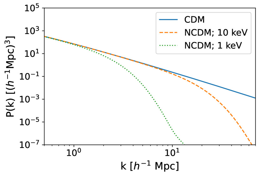
Figure 1: Examples of the input 3D matter power spectra for the simulations. We can see NCDM suppresses the amplitude of the power spectrum on small scales.

Dark matter has a non-zero mass but interacts with electromagnetic radiation very weakly, if at all. Consequently, dark matter cannot be observed directly and can only be detected by its gravitational interactions. The structure formation in the universe is influenced by the gravity of dark matter, so observing the large-scale structure of the universe provides information about dark matter.

This paper considers two types of dark matter: cold dark matter (CDM) and non-cold dark matter (NCDM). CDM is a heavy particle that was non-relativistic at the time of freeze-out, resulting in a negligible velocity dispersion. In contrast, NCDM is a lighter particle with a significant velocity dispersion.

Dark matter’s velocity dispersion impedes the growth of structure, particularly on small scales. The velocity dispersion is inversely proportional to the mass of the dark matter particle, $m_{\rm DM}$. Consequently, the damping scale of the matter power spectrum resulting from this velocity dispersion is also $\propto 1/m_{\rm DM}$ Boyanovsky2011 (See Fig. 1).

We calculate the matter power spectra for both the CDM and NCDM models with different particle masses using the Cosmic Linear Anisotropy Solving System (CLASS) Lesgourgues2011a . Our NCDM model considers the sterile neutrino, a fundamental particle added to the standard model and distinct from active neutrinos (electron, mu, and tau neutrinos). CLASS uses the energy distribution function of dark matter based on the widely studied sterile neutrino model Dodelson1994 and calculates the time evolution of density perturbations, fluid-velocity divergence, and shear stress in the phase space using the fluid approximation Lesgourgues2011b (see Section 3 in Lesgourgues2011b ).

In this work, in addition to the CDM model, we consider the NCDM model with particle masses $m_{\rm DM}$ uniformly sampled in logarithmic scale from $10^{3}$ to $10^{5}$ eV. We do not consider the case of $10^{5}$ eV as it is indistinguishable from the CDM model using any of the methods described in this paper.

II.2 HI Distribution and Differential Brightness Temperature

This work focuses on the HI gas distribution as a tracer of the dark matter distribution. In this subsection, we demonstrate the relationship between the HI density and the brightness differential temperature $\delta T_{b}$ which is the observable quantity. We consider only the epoch well after reionization, during which most of the hydrogen has already been ionized.

$\delta T_{b}$ is the difference between the temperatures of the 21cm radiation and the cosmic microwave background, $T_{\gamma}$ Field1958 ,

$$\delta T_{b}=\frac{T_{\rm S}-T_{\gamma}(z)}{1+z}(1-e^{-\tau_{\nu_{0}}}),$$ (1)

where $\nu_{0}=1420$ MHz is the frequency of 21cm radiation at the rest frame, $T_{\rm S}$ is the spin temperature of HI, and $z$ is the redshift of the source of the 21cm radiation. The optical depth of HI can be given by,

$$\tau_{\nu_{0}}=\frac{3}{32\pi}\frac{h_{p}c^{3}A_{10}}{k_{\rm B}T_{S}\nu^{2}_{0}}\frac{n_{\rm HI}}{(1+z)(dv_{\parallel}/dr_{\parallel})},$$ (2)

where $n_{\rm HI}$ is the HI number density, and $dv_{\parallel}/dr_{\parallel}$ is the velocity gradient of the HI gas along the line of sight. We replace it with the $H(z)$ because the peculiar velocity is small enough compared to the Hubble expansion (Ando2021, ). We can also assume $\tau\ll 1$, and thus we have

$$\delta T_{b}\sim\frac{3}{32\pi}\frac{h_{p}c^{3}A_{10}}{k_{\rm B}\nu^{2}_{0}}\left(1-\frac{T_{\gamma}(z)}{T_{\rm S}}\right)\frac{n_{\rm HI}}{(1+z)H(z)}.$$ (3)

The spin temperature is Field1958

$$T^{-1}_{\rm S}=\frac{T^{-1}_{\gamma}+x_{\alpha}T^{-1}_{\alpha}+x_{c}T^{-1}_{\rm K}}{1+x_{\alpha}+x_{c}},$$ (4)

where $T_{\alpha}$ and $x_{\alpha}$ is the temperature of Ly-$\alpha$ and its coupling coefficient, and $T_{\rm K}$ and $x_{c}$ is the kinetic gas temperature and its coefficient. We calculate these values following (Furlanetto2006, ; Endo2020, ).

II.3 Implementation to Hydrodynamic Simulation

We perform a series of hydrodynamic simulations for dark matter models with different particle masses. For the range of the value of $m_{\rm DM}$ under consideration, all dark matter particles only interact gravitationally after the initial condition is generated at redshift $z=99$. All the features of dark matter models can be encoded in the matter power spectrum at the initial condition. We use the cosmological parameters obtained by Planck Akrami2018 as $\Omega_{m}=0.311,\ \Omega_{\Lambda}=0.689,\ \Omega_{b}=0.049,\ h=0.677,$ and $\ln 10^{10}A_{s}=3.047$ in the CDM model. In addition to the standard CDM model, we consider NCDM (non-CDM) models with six different particle masses logarithmically sampled from $10^{3}$ to $10^{4.66}$ eV. We only consider a single dark matter component in each case.

The matter power spectrum for the initial condition of the hydrodynamic simulation is calculated by CLASS (Lesgourgues2011a, ), as shown in Fig. 1. Using these input power spectra, we generate the initial conditions with 2LPTic (Crocce2006, ), followed by applying glass realization to remove the grid pattern in the particle distribution. While the value of AUC (introduced in Section III.3.2) increases slightly by $\sim\mathcal{O}(0.01)$ with the grid realization, it produces unrealistic features in the matter distribution for NCDM simulations Gotz2002 ; Gotz2003 .

We use GADGET3-Osaka 10.1093/mnras/stw3061 ; 10.1093/mnras/stz098 to solve the evolution of the matter distribution. It is a cosmological smoothed particle hydrodynamics (SPH) code based on GADGET-3 (originally described in Springel2005 ), which we modified. Our simulations use a comoving box size of 100 $h^{-1}$Mpc on a side, with $512^{3}$ dark matter and $512^{3}$ gas particles. We generate the initial conditions at $z=99$ and terminate the simulation at $z=3$. This code includes models for star formation, supernova feedback, UV radiation background, and radiative cooling/heating. We also include the effect of self-shielding of HI gas, which is the obstruction of UV radiation by optically thick HI gas. The cooling is solved by using the Grackle chemistry and cooling library grackle .

For the Fiducial model, we adopt the star formation model used in the AGORA project Kim_2014 ; Kim_2016 , supernova feedback described in 10.1093/mnras/stz098 , and the uniform UV radiation background Haardt_2012 without the effect of the self-shielding of HI gas. For the Fiducial model, we conduct 7 simulations, CDM and 6 NCDM.

We examine if the effects of astrophysical models and dark matter models are distinguishable or not. For this purpose, we conduct three additional simulations for CDM with different astrophysical models where a part of the assumptions is different from the Fiducial model. The Shield model includes the effect of self-shielding of the HI gas, the NoSF model ignores the effect of star formation, and the FG09 model adopts the UV radiation background model of Faucher_Gigu_re_2009 instead of Haardt_2012 . The details of Fiducial, Shield, and FG09 models are discussed in Nagamine_2021 .

II.4 Training and Test Sets

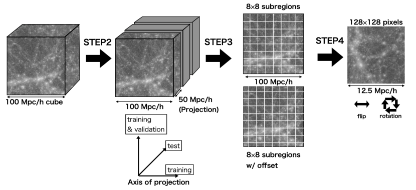
Figure 2: The procedure for making images from our simulation data.

Figure 3: Example images of the CDM, 21 keV NCDM, and 1 keV NCDM models from the left to right. The upper panels show dark matter images and the lower panels show $\delta T_{b}$ images which are the logarithm of the actual images for visibility. These images are made from the same region of the simulation box.

In this subsection, we describe the procedures for generating the images from the hydrodynamic simulation used for the training, validation, and testing of CNN. The scale of the damping of the power spectrum due to the velocity dispersion of NCDM is $k\sim 1\ h\mathrm{Mpc}^{-1}$ for $10^{3}$ eV and $k\sim 50\ h\mathrm{Mpc}^{-1}$ for $10^{4.66}$ eV in Fourier space. Therefore, the image size should be sufficiently large to include the mode $k\sim 1\ h\mathrm{Mpc}^{-1}$, and at the same time, it should have sufficient resolution to resolve $k\sim 50\ h\mathrm{Mpc}^{-1}$ mode fluctuations. Our box size and the number of particles satisfy these requirements.

To generate images from an hydrodynamic simulation, we implement the following procedures (see Fig. 2):

• [STEP 1] We define a $1024^{3}$ grid in the simulation box and redistribute the dark matter particles to the nearest grid point or calculate the HI number density in each grid using the SPH kernel. The smaller scale than the size of this grid is dominated by the SKA-MID system noise. We compute the SPH kernel following the cubic spline kernel Monaghan_1985 as

  $$W_{\rm SPH}(r,h)$$

  $$=A\begin{cases}1-\frac{2}{3}\left(\frac{r}{h/2}\right)^{2}+\frac{3}{4}\left(\frac{r}{h/2}\right)^{3}&(0<r<\frac{h}{2})\\ \frac{1}{4}\left(2-\frac{r}{h/2}\right)^{3}&(\frac{h}{2}<r<h)\\ 0&(h<r)\ ,\end{cases}$$ (5)

  where $h$ is the smoothing length for each particle and $r$ is the distance between the particle and the center of the cell. The amplitude $A$ is determined so that for every particle, the sum of $W_{\rm SPH}$ over all grid becomes unity. The HI number density $n_{\rm HI}$ in a grid whose center is located at $\mbox{\boldmath${x}$}_{i}$ is calculated by summing over all particles contributing to this grid,

  $$n_{\rm HI}(\mbox{\boldmath${x}$}_{i})=\sum_{j}W_{\rm SPH}(\mbox{\boldmath${x}$}_{i}-\mbox{\boldmath${x}$}_{j}|h_{j})n_{\mathrm{HI},j}$$ (6)

  where $n_{\mathrm{HI},j}$ is the HI number density assigned to the $j$-th particle located at $\mbox{\boldmath${x}$}_{j}$. And then, we calculate the $\delta T_{b}$ by Eq. (3).

• [STEP 2] We divide the simulation box into three slices along the line of sight with each width being $50$ $h^{-1}$Mpc. Each piece corresponds to the region of the simulation box from 0 to 50 $h^{-1}$Mpc, from 25 to 75 $h^{-1}$Mpc, and from 50 to 100 $h^{-1}$Mpc along the line of sight. We investigate the optimal length of the slice from 50 $h^{-1}$Mpc (limited by the number of images for the sufficient training of CNN) to 0.1 $h^{-1}$Mpc (limited by the size of the cell in STEP 1), and find that AUC (introduced in Section III.3.2) for the classification between the CDM and 10 keV NCDM model is maximized when we define the projection depth as 50 $h^{-1}$Mpc. We have three degrees of freedom for the line-of-sight direction; these can be considered independent realizations. Therefore, we have (3 line-of-sight directions) $\times$ (3 slices) $=9$ slices of the simulation. We use the images generated from the five slices as the training data and the ones from the other slice as the validation data for the two line of sight directions. And the, we use the images from the three slices of the other line of sight direction as the test data.

• [STEP 3] Within each sub-region, the mass density of dark matter $\rho_{\rm DM}(\mbox{\boldmath${x}$})$ is integrated along the line of sight and projected onto the plane perpendicular to line of sight, i.e, $\rho_{\rm DM}(\mbox{\boldmath${n}$})=\int\rho_{\rm DM}(\mbox{\boldmath${x}$})dx$ where $\rho_{\rm DM}(\mbox{\boldmath${n}$})$ is the 2D mass density of dark matter at the position ${n}$ on the 2D plane. And then, we calculate the 2D density fluctuation $\delta_{\rm DM}(\mbox{\boldmath${n}$})=(\rho_{\rm DM}(\mbox{\boldmath${n}$})-\bar{\rho}_{\rm DM})/\bar{\rho}_{\rm DM}$ for dark matter, where $\bar{\rho}$ is the mean $\rho_{\rm DM}(\bm{n})$ over the simulation box. For HI, $\delta T_{b}$ is summed up along with the line of sight, i.e., $\delta T_{b}(\mbox{\boldmath${n}$})=\sum_{\rm los}\delta T_{b}(\mbox{\boldmath${x}$})$.

• [STEP 4] In each slice, we cut out 8$\times$8 images, therefore, the single image has 128² pixels, 12.5 $h^{-1}$Mpc on a side, which is sufficiently larger scale than $k\sim 1h\mathrm{Mpc}^{-1}$. For the data augmentation, we employ multiple offsets when we subdivide the slices for making the training or validation data. The offsets are $\Delta=12.5i/16$ $h^{-1}$Mpc where $i=0,1,\cdots,15$ both in the directions parallel or perpendicular to a side. At the edge of the slice, we apply the periodic boundary condition. This may increase the number of available images sufficiently and significantly help our training process to converge, although the shifted images are not totally independent of each other.

In total, we have (5, 1, or 3 slices in Step 2) $\times$ ($16^{2}$, $16^{2}$, or $1$ (no offset)) = 81,920, 16,384, or 192 images for each training, validation, or test data for one realization of the simulation. In addition, in training the CNN, the images are rotated every 90 degrees and flipped horizontally to generate another different set of images. Thus, the number of training data is effectively $81920$ $\times$ ($2$ flips) $\times$ ($4$ rotation) $=655,360$; however, in testing our CNN, test images are not flipped or rotated.

The images for training and test is not completely independent and there is a possibility that it has effects on the results because they are from the same realization. To confirm whether the test images made from the same realization used to make training images are valid, we prepare the another realization for Fiducial CDM and 10 keV NCDM model. And then, we make 192 images from each these new realizations on the same procedure above, and use them to test our CNN trained by the training dataset from the original realization. As a result, AUC for the images from the new realizations is 0.80 and consistent with the result AUC=0.78 for the test images made from the same realization as for the training images (see also Section IV.1).

The image of density fluctuation $\delta$ has large dynamic ranges due to the non-linear evolution of the structure. For our neural network architecture, it is difficult to extract feature quantities from such high dynamic range images; therefore, we apply the transformation

$$\delta^{\prime}(x)={\rm arcsinh}[\delta(x)].$$ (7)

This transformation is motivated by the magnitude system, Luptitude introduced by the Sloan Digital Sky Survey (Lupton+:1999, ). This is particularly useful for reducing the dynamic range, including negative values to which a simple logarithmic scale cannot be applied.

III Method

III.1 Power Spectrum

In many cases of cosmological inference, the clustering analysis is mainly quantified through the two-point statistics such as power spectrum or correlation function in the literature because of the great success of the linear perturbation theory and inflation model to predict the Gaussian initial density field. However, the non-linear gravitational evolution of the structure carries additional information than two-point statistics. In this section, we revisit the basic methodology of the power spectrum-based analysis. Note that, unlike the parameter inferences in which we compare the data with the prediction, here we focus on the classification problem: whether we can distinguish the power spectra of NCDM from the Fiducial power spectrum of CDM. Two dimensional Fourier counterpart $\tilde{A}(\mbox{\boldmath${k}$})$ of a physical quantity $A(\mbox{\boldmath${n}$})$ at the position ${n}$ on a 2D plane is written as

$$\tilde{A}(\mbox{\boldmath${k}$})=\int\exp{(-i\mbox{\boldmath${k}$}\cdot\mbox{\boldmath${n}$})}A(\mbox{\boldmath${n}$})d^{2}n,$$ (8)

where the unit of $\tilde{A}$ is the unit of $A$ multiplied by $(h^{-1}\mathrm{Mpc})^{2}$. And then, using the simulation, the power spectrum for the projected field along the line of sight for dark matter is

$$P^{\rm DM}(k_{i})\ [(h^{-1}\mathrm{Mpc})^{2}]=\frac{1}{L^{2}}\frac{1}{N_{k_{i}}}\sum_{j}\tilde{\delta}_{\rm DM}(\mbox{\boldmath${k}$}_{j})\tilde{\delta}_{\rm DM}^{*}(\mbox{\boldmath${k}$}_{j}),$$ (9)

and the one for the $\delta T_{b}$ is

$$P^{\rm\delta T_{b}}(k_{i})\ [\mathrm{mK}^{2}(h^{-1}\mathrm{Mpc})^{2}]=\frac{1}{L^{2}}\frac{1}{N_{k_{i}}}\sum_{j}\tilde{\delta T_{b}}(\mbox{\boldmath${k}$}_{j})\tilde{\delta T_{b}}^{*}(\mbox{\boldmath${k}$}_{j}),$$ (10)

where $\tilde{\delta}_{\rm DM}$ and $\tilde{\delta T_{b}}$ are two dimensional Fourier counterparts of $\delta_{\rm DM}$ and $\delta T_{b}$ respectively, $k_{i}=|\mbox{\boldmath${k}$}_{i}|$ is the absolute value of the wave number of the center of the $i$-th bin, $\mbox{\boldmath${k}$}_{j}$ is the wave number satisfies $k_{i}\leq|\mbox{\boldmath${k}$}_{j}|<k_{i+1}$, $N_{k_{i}}$ is the number of the modes in $i$-th $k$ bin, and $L$ is the size of image and is 12.5 $h^{-1}$Mpc. The factor $1/L^{2}$ is due to the finite interval of integration in Fourier transform ($L\rightarrow 2\pi$ if the image size is infinite). The minimum and maximum wavenumbers are automatically determined by the size and resolution of the images from which we measure the spectrum, and they are $k_{\rm min}=2\pi/12.5\ h\mathrm{Mpc}^{-1}$ and $k_{\rm max}=2\pi/(12.5/128)\ h\mathrm{Mpc}^{-1}$, respectively. We change the number of $k$-bins from 1 to 20, and find that 4 is optimal in terms of the classification performance of the power spectrum.

The covariance matrix of the power spectrum can be measured from test images of the CDM simulation,

$$C_{mn}=\frac{1}{N_{\rm img}}\sum_{l}\left(P_{l}(k_{m})-\bar{P}(k_{m})\right)\left(P_{l}(k_{n})-\bar{P}(k_{n})\right),$$ (11)

where the subscript $l$ is the label of the test images, $N_{\rm img}(=192)$ is the number of the test images from CDM simulation data, and $\bar{P}(k)=\sum_{l}P_{l}(k)/N_{\rm img}$ is the mean of the power spectra of the CDM test image.

III.2 Convolutional Neural Network

	Layer	Output map size
1	Input	$128\times 128\times 1$
2	$3\times 3$ convolution	$126\times 126\times 32$
3	$3\times 3$ convolution	$124\times 124\times 32$
4	$3\times 3$ convolution	$122\times 122\times 64$
5	$3\times 3$ convolution	$120\times 120\times 64$
6	$3\times 3$ convolution	$118\times 118\times 128$
7	$1\times 1$ convolution	$118\times 118\times 64$
8	$3\times 3$ convolution	$116\times 116\times 128$
9	$2\times 2$ AveragePooling	$58\times 58\times 128$
10	$3\times 3$ convolution	$56\times 56\times 256$
11	$1\times 1$ convolution	$56\times 56\times 128$
12	$3\times 3$ convolution	$54\times 54\times 256$
13	$2\times 2$ AveragePooling	$27\times 27\times 256$
14	$3\times 3$ convolution	$25\times 25\times 512$
15	$1\times 1$ convolution	$25\times 25\times 256$
16	$3\times 3$ convolution	$23\times 23\times 512$
17	$2\times 2$ AveragePooling	$12\times 12\times 512$
18	$3\times 3$ convolution	$10\times 10\times 512$
19	$1\times 1$ convolution	$10\times 10\times 256$
20	$3\times 3$ convolution	$8\times 8\times 512$
21	$1\times 1$ convolution	$8\times 8\times 256$
22	$3\times 3$ convolution	$6\times 6\times 512$
23	GlobalAveragePooling	1 $\times$ 1 $\times$ 512
24	FullyConnected	2

Table 1: Our CNN architecture. The second column shows the type of layer and the third column shows the size of the output from the layer ((height $\times$ width $\times$ channel) of the feature map). The total number of trainable parameters is 8,328,610.

In this section, we describe our CNN model. In our model, we apply convolution layers with $3\times 3$ kernels for deep multiple layers to extract characteristics over various scales from images. We use the publicly available platform PyTorchpytorch to construct our model. We follow the previous work Ribli2019a for the architecture of the neural network except that we skip the first two Average Pooling layers in Ribli2019a because the size of the input image is different. The architecture is summarized in Table 1. The total number of trainable parameters in this architecture is $\sim 8\times 10^{6}$; therefore, $10^{5}$ images are required to avoid both over- and under-fitting of the data Han2015 . Therefore, we prepare $6\times 10^{5}$ images for each simulation.

We try to find the optimal number of layers, and it is summarized in Table 1. If we halve the number of layers by skipping all of the 4th, 5th, 6th, 12th, 16th, and 22nd layers in Table 1, the losses, computed by Eq. (14), gets 10 times larger and the validation accuracy is $\sim 0.5$, which means the model prediction is totally random and not able to classify the inputs. This is because this model is too simple. Conversely, if we double the number of layers by repeating each convolution layer twice with zero-padding to keep the size of the feature map unchanged, the loss does not decrease during the optimization. This is because the number of trainable parameters is too large compared to the size of our training dataset and the vanishing gradients may occur 2015arXiv151203385H . Again, we observe that the validation accuracy fluctuates around 0.5.

Now we explain the detailed procedures in each layer. In general, $n_{x}\times n_{y}$ convolution kernel translates the $N_{x}\times N_{y}$ input image into $(N_{x}-(n_{x}-s_{x}))\times(N_{y}-(n_{y}-s_{y}))$ image, when the stride is $s_{x}\times s_{y}$ and no-padding is applied. In our analysis, we always fix $s_{x}=s_{y}=1$. The number of output feature maps depends on the number of kernels in the current layers which can vary from 1 to 512 in our analysis. The kernel values are initially set randomly but they are subject to be optimized during the training process. After each convolution layer, we add a batch-normalization layer to normalize the distribution of the input feature map, which increases the training efficiency (2015arXiv150203167I, ). Also, after every convolution layer, we apply an activation function of ReLU ReLU .

In the $n_{x}\times n_{y}$ AveragePooling layer, when we set the stride to be the same as $n_{x}$ and $n_{y}$, then $N_{x}\times N_{y}$ input image is converted into an $(N_{x}/n_{x})\times(N_{y}/n_{y})$ image. In these layers, the information in the input image is compressed and simplified. In the GlobalAveragePooling layer, the values of all pixels in each input map are averaged. We find that the combination of the GlobalAveragePooling and the single FullyConnected layers shows better performance than the multiple FullyConnected layers. Finally, the FullyConnected layer adopts the softmax activation function as the final output of the model, which is the probabilities of the input image being CDM or NCDM models respectively.

Now, we can express the outputs in relation to the input and predicted classes,

$$\bm{p}_{i}(\mathrm{M})=\{p_{i}(\mathrm{CDM}|\mathrm{M}),p_{i}(\mathrm{NCDM}|\mathrm{M})\},$$ (12)

where $p_{i}(k|\rm M)$ is the probability predicted by our CNN that the $i$-th input image is $k(=\rm CDM\ or\ NCDM)$ model and M means the true dark matter model for the $i$-th input. This is converted from the output of the last FullyConnected layer $\bm{y}({\rm M})=\{y_{i}(k|{\rm M}),y_{i}(k|{\rm M})\}$ by the softmax function;

$$p_{i}(k|\mathrm{M})=\frac{\exp{(y_{i}(k|\mathrm{M}))}}{\exp{(y_{i}({\rm CDM}|\mathrm{M}))}+\exp{(y_{i}({\rm NCDM}|\mathrm{M}))}}.$$ (13)

For loss function, we adopt a typical cross-entropy

$$E_{i}(\bm{w})=-\sum_{k}\tilde{p}_{i}({k|{\rm M}})\ln{(p_{i}(k|{\rm M}))}.$$ (14)

In this equation, the ground truth $\tilde{p}_{i}$ takes 1 for correct class ($k={\rm M}$) and 0 otherwise ($k\neq{\rm M}$), and prediction $p_{i}$ takes continuous values between 0 and 1. The output $p_{i}$ is an implicit function of $\bm{w}$, which is subject to be optimized.

For optimization purposes, we use the AMSGRADAMSGRAD , and take the learning rate as $10^{-5}$. The updates of the trainable parameters are computed based on the averaged value of the loss function $\bar{E}$ over the mini-batch sample, which is randomly drawn from the training dataset. We take 8 mini-batch samples for better convergence of the training. The validation sample generated as Section II.4 is used for evaluating the training. The convergence condition is that the validation loss averaged over the latest 5 epochs converges to 1%.

III.3 Evaluation of Classification

In the following of this paper, we consider the binary classification between the images from the CDM model and the NCDM model. In this subsection, we introduce the Kolmogorov-Smirnov (KS) test, which is used to evaluate the results of the classification both by CNN and power spectrum. In addition to this, for image classification, we also use AUC to quantify the goodness of the prediction model.

III.3.1 Kolmogolov-Smirnov Test

The KS test evaluates whether the underlying distribution functions for two distinct finite samples are the same KS_1 ; smirnov1939estimate . In our analysis, we adopt the KS test to discriminate the images or power spectra of CDM and NCDM models.

We use the distributions of the $\chi^{2}$ values of the power spectra and the outputs from our CNN. For the $i$-th test image of dark matter model M, we calculate the $\chi^{2}$ value of the power spectrum as

$$\chi^{2}_{{\rm PS},i}(\rm{M}) =\bm{\Delta}P_{i}(k|\mathrm{M})\bm{\mathrm{C}}^{-1}\bm{\Delta}P_{i}(k|\mathrm{M}),$$ (15)

where $\bm{\Delta}P_{i}(k|\mathrm{M})=P_{i}(k|\mathrm{M})-\bar{P}(k|\mathrm{CDM})$ is the power spectrum difference of the $i$-th input image of the dark matter model M defined by Eq. (9) or Eq. (10), $\bar{P}(k)$ is the power spectrum averaged over the CDM images and $\boldmath{\mathrm{C}}^{-1}$ is the inverse of the covariance matrix defined in Eq. (11). For the case of image classification, we have defined the discriminator that quantifies the difference between two dark matter models,

$$\chi^{2}_{\mathrm{CNN},i}(\mathrm{M})=\frac{(y_{i}(\mathrm{M})-\bar{y}(\mathrm{CDM}))^{2}}{\frac{1}{N}\displaystyle\sum_{j}\left(y_{j}(\mathrm{CDM})-\bar{y}(\mathrm{CDM})\right)^{2}},$$ (16)

where $y_{i}(M)$ is the prediction of CNN that the $i$-th input image of dark matter model M to be the NCDM model, where $M$ is either CDM or NCDM. $\bar{y}(\mathrm{CDM})$ is the average of $y_{i}({\rm CDM})$ over the CDM test images and the denominator of the right-hand side of Eq.(16) is the variance of the CNN outputs for CDM input images.

And then, we conduct the KS test for the distribution of $\chi^{2}_{i}(\mathrm{CDM})$ and $\chi^{2}_{i}(\mathrm{NCDM})$ with stats.ks_2samp method in SciPyscipy . The null hypothesis of our test is that there is no significant difference between the distribution of the $\chi^{2}$ for the CDM images and the NCDM images. We use the $p$-value = 0.01 ($\sim 2.6\sigma$) as the significance level in this work.

We note that the KS test employed here only tells us whether or not there is a significant difference between images of two different models, and thus it is not able to quantify whether the output model is correct or not. In order to further quantify this, we will introduce AUC in the next section.

III.3.2 AUC

The area under the Receiver Operating Characteristic (ROC) curve is used to quantify the ability of the CNN model to correctly predict the dark matter model.

The output of the CNN is the probability of the input image being the NCDM model. For binary classification, we need to define a certain threshold $t$ such that the CNN can recognize the input image as the NCDM model if $p_{i}>t$. Therefore, we can explicitly consider the four different cases: (1) True Positive (TP) if $p_{i}(\mathrm{NCDM}|\mathrm{NCDM})\geq t$, (2) True Negative (TN) if $p_{i}(\mathrm{NCDM}|\mathrm{CDM})<t$, (3) False Positive (FP) if $p_{i}(\mathrm{NCDM}|\mathrm{CDM})\geq t$ and (4) False Negative (FN) if $p_{i}(\mathrm{NCDM}|\mathrm{NCDM})<t$, where all four quantities are a function of $t$.

Now, the ROC curve can be defined as the collection of points at which parameter $t$ continuously changes from 0 to 1. More specifically, it can be expressed in a parametric manner,

$$\mathrm{ROC}:x(t)=\frac{\rm FP}{\rm TN+FP},\quad y(t)=\frac{\rm TP}{\rm TP+FN},$$ (17)

where $x$ represents the fraction of misclassified images as the NCDM model out of all CDM test images and $y$ represents the fraction of correctly classified images as the NCDM model given all NCDM inputs. Therefore, the area under the curve (AUC) approaches unity when the classification is both efficient and complete.

IV Results

In this section, we show the results of the dark matter model classification between CDM and NCDM whose particle mass is $m_{\rm DM}$ by use of image-based CNN and compare it with the power spectrum-based classification. In Section IV.1, we show the results for dark matter density field images and compare them with the power spectrum classification. We further extend the same analysis to the $\delta T_{b}$ field which is the indirect probe of dark matter but a direct observable. In Section IV.2, we explore how the results are affected by the nuisance effects caused by the astrophysical feedback. Finally, in Section IV.3 we also consider the realistic system noise of the SKA-MID instruments which can weaken the constraints.

IV.1 Comparison between dark matter and $\delta T_{b}$ image

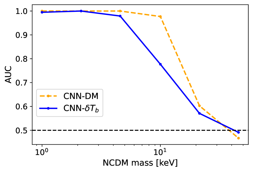
Figure 4: AUC as a function of $m_{\rm DM}$ for dark matter images (blue solid) and $\delta T_{b}$ images (orange dashed). The dashed horizontal line represents the case of random classification. We see CNN-DM shows better performance than CNN-$\delta T_{b}$.

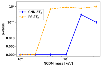
Figure 5: The comparison of the dark matter model classifications probed by the $p$-value of the KS test. The horizontal axis is the mass of NCDM and the vertical axis is the $p$-value for PS-DM (orange dashed) and CNN-DM (blue solid) in the left panel, and for PS-$\delta T_{b}$ (orange dashed) and CNN-$\delta T_{b}$ (blue solid) in the right panel. We see that CNN has a significantly better $p$-value than the power spectrum for both the classification of dark matter and $\delta T_{b}$ images.

For latter convenience, we first define the acronyms X-Y denoting the observable Y is classified by the method X, where X is either CNN or PS and Y is either DM or $\delta T_{b}$. For e.g. CNN-$\delta T_{b}$ stands for the image-based classification using the $\delta T_{b}$ map.

First, we show the comparison between the result of CNN-DM and CNN-$\delta T_{b}$. In Fig. 4, we see that for both dark matter and $\delta T_{b}$ images, AUCs are greater than 0.95 at mass ranges of $m_{\rm DM}\leq 2.1$ keV. Once the dark matter mass is 10 keV, the difference becomes prominent. The CNN-DM can still constrain the model with a high AUC, 0.97 but the CNN-$\delta T_{b}$ dramatically lose its discrimination power down to AUC=0.78. This can be naturally explained that the $\delta T_{b}$ is an indirect probe of dark matter and thus the free streaming of NCDM is reflected less prominently compared to the dark matter distribution.

Next, we compare the discrimination power between CNN and PS for dark matter or $\delta T_{b}$ using the KS test. Fig. 5 shows the $p$-value of the KS test for the classification of dark matter data in the left panel and $\delta T_{b}$ data in the right panel. We see that our CNN shows better performance than the power spectrum for both dark matter and $\delta T_{b}$ data. For example, $p$-value of CNN-DM and CNN-$\delta T_{b}$ at $m_{\rm DM}=4.6$ keV is less than $0.001$ and can reject the null hypothesis with high significance while the $p$-value of PS-DM and PS-$\delta T_{b}$ is of the order of 0.1.

Now we compare the results of CNN-DM and CNN-$\delta T_{b}$. Unlike the AUC analysis, they show similar performance for the KS test. Both of them can classify the images for $m_{\rm DM}\leq 10$ keV with high significance ($p$-value $<0.001$, and lose the classification ability for more massive dark matter (e.g. the $p$-values of CNN-DM and CNN-$\delta T_{b}$ are 0.37 and 0.30 at $m_{\rm DM}=$ 21 keV). Therefore, AUC$=0.78$ which is the value from CNN-$\delta T_{b}$ for $m_{\rm DM}=10$ keV is enough high for the classification. As we have seen in the AUC analysis, CNN-$\delta T_{b}$ takes significantly lower discrimination ability compared to the CNN-DM at $m_{\rm DM}=10$ keV, however; the CNN is still able to recognize that the two dark matter models are different.

IV.2 Effect of Astrophysical Model

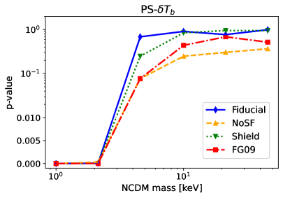
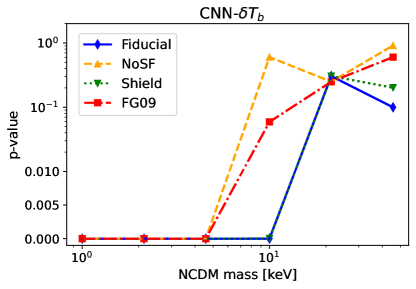
Figure 6: The $p$-values of the KS test including the results for the various astrophysical models. The horizontal axis is the NCDM mass, and the vertical axis shows the $p$-value for the binary classification by PS-$\delta T_{b}$ (left panel) or CNN-$\delta T_{b}$ (right panel) between the NCDM and the CDM assumed the Fiducial (blue solid), NoSF (orange dashed), Shield (green dotted), and FG09 (red dashed-dotted) model. We can see the difference according to the astrophysical model has an effect on the classification for $m_{\rm DM}\geq 10$ keV for CNN classification.

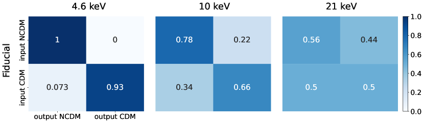
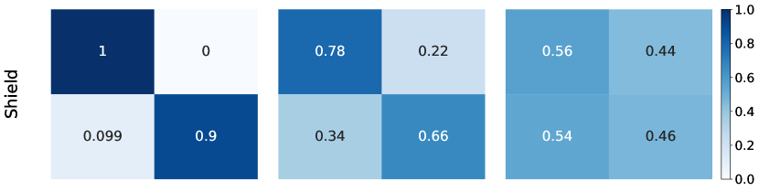
Figure 7: This figure shows the confusion matrix. Each column corresponds to the NCDM mass $m_{\rm DM}=4.6,10,$ and $21$ keV from left to right, and each row corresponds to the astrophysical model: Fiducial, Shield, NoSF, and FG09 from top to bottom. For the Shield model, the confusion matrix is almost the same as for the Fiducial model. On the other hand, in the case of the NoSF or FG09 model, the number of CDM test images classified incorrectly is increased.

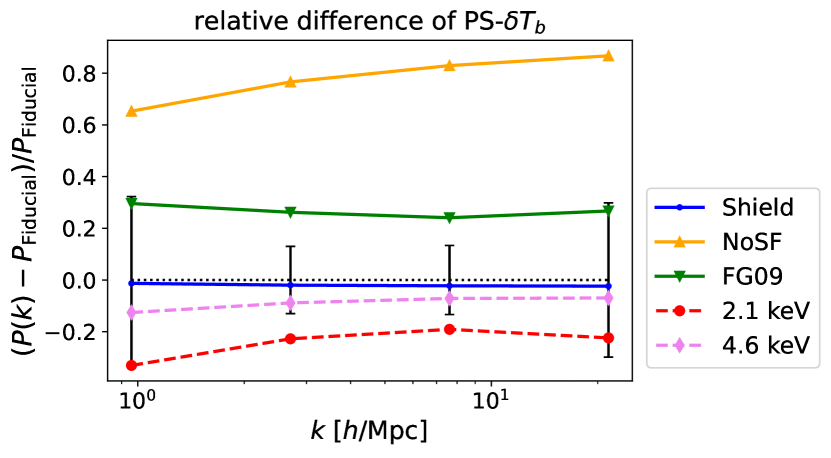
Figure 8: Relative difference between the $\delta T_{b}$ 2D power spectrum with Shield (blue solid), NoSF (orange solid), FG09 (green solid), 2.1 keV (violet dashed) or 4.6 keV (red dashed) model and Fiducial CDM model. The dotted black horizontal line represents unity with 1$\sigma$ error which includes the statistical error of the Gaussian power spectrum and the system noise introduced in Section IV.3 with $t_{0}=1,000$ hours. We can see that the power spectrum for the different astrophysical models is amplified relative to the Fiducial model, while that of the NCDM models is suppressed.

In this subsection, we investigate the effect of the different astrophysical models on the classification. In order to quantify the effect, we simply replace the CDM test images with the images generated from the simulations of different astrophysical models, i.e., the Fiducial model is replaced with one of FG09, Shield, or NoSF models. In the following, we only consider the analysis of $\delta T_{b}$ images.

Fig. 6 shows the $p$-values of the KS test for different astrophysical models for PS-$\delta T_{b}$ (left) and CNN-$\delta T_{b}$ (right). For PS-$\delta T_{b}$, the $p$-value $<0.01$ for $m_{\rm DM}\leq 2.1$ keV independent of the astrophysical models. For $m_{\rm DM}\geq 4.6$ keV, $p$-value is more than 0.1 , so the power spectrum cannot distinguish different dark matter models and the difference according to the astrophysical models is not significant in our power spectrum analysis.

Next, for CNN, the right panel of Fig. 6 shows the $p$-value for CNN-$\delta T_{b}$. We see that for $m_{\rm DM}\leq 4.6$ keV, CNN can discriminate the dark matter models regardless of the astrophysical models. For $m_{\rm DM}=10$ keV, the $p$-values for NoSF and FG09 inflate but for Fiducial and Shield models, it still remains close to zero, $p<0.01$. Therefore, the results indicate that the difference in the density maps between CDM and NCDM is partly mimicked by the astrophysical effects of the star formation or inhomogeneous UV background. Conversely, for the mass ranges of $m_{\rm DM}<4.6$ keV, we do not observe the astrophysical effect spoils the classification, and thus we can conclude that the classification for $m_{\rm DM}<4.6$ keV is robust against the astrophysical models at least within the models we consider in our simulation.

Model	4.6 keV	10 keV	21 keV
Fiducial	0.98	0.78	0.57
Shield	0.98	0.76	0.57
NoSF	0.96	0.64	0.51
FG09	0.95	0.66	0.52

Table 2: The values of AUC for the classifications. Each row corresponds to the astrophysical model; Fiducial, Shield, NoSF, FG09, and each column corresponds to NCDM mass $m_{\rm DM}=$ 4.6 keV, 10 keV, 21 keV NCDM model. The value of AUC is decreased if we assume the wrong astrophysical model for $m_{\rm DM}\geq 10$ keV.

In what follows, we will discuss the effect of astrophysical models on CNN analysis. We quantify the effect using the AUC and confusion matrix. The confusion matrix is defined as

$$\left(\begin{array}[]{crl}\displaystyle\frac{\mathrm{TP}}{\mathrm{TP}+\mathrm{FN}}&\displaystyle\frac{\mathrm{FN}}{\mathrm{TP}+\mathrm{FN}}\\ \\ \displaystyle\frac{\mathrm{FP}}{\mathrm{TN}+\mathrm{FP}}&\displaystyle\frac{\mathrm{TN}}{\mathrm{TN}+\mathrm{FP}}\\ \end{array}\right),$$ (18)

where TP, FN, TN, and FP are evaluated at threshold $t=0.5$. The upper left and right elements are the rate of the correct and incorrect classification for the NCDM test images, and lower left and right elements are the rate of the correct and incorrect classification for the CDM test images, respectively.

Fig. 7 and Table. 2 show the confusion matrix and AUC, respectively. The left, middle, and right columns correspond to the classification for $m_{\rm DM}=4.6,10,$ and $21$ keV respectively, and each row from top to bottom corresponds to the Fiducial, Shield, NoSF, and FG09 model in Fig. 7. We see that there is little difference between the Fiducial and Shield model in the confusion matrix and AUC. On the other hand, for the NoSF or FG09 models, the fraction of misclassified as NCDM (the lower left element) increases and AUC decreases for 10 and 21 keV. For example, for $m_{\rm DM}=$10 keV, the fraction of misclassified as NCDM is 0.58 (NoSF) and 0.57 (FG09), which is larger than 0.34 (Fiducial).

Also, the AUC is 0.64 for NoSF and 0.66 for FG09, which is worse than 0.78 for Fiducial model. This implies that the number of CDM test images correctly classified as CDM decreases if we assume the wrong astrophysical model. These results are consistent with the results from the KS test, i.e., the performance of the classification by CNN is degraded if we assume the wrong astrophysical model.

We explore how the power spectrum changes depending on the different astrophysical models. Fig. 8 shows the fractional difference of 2-dimensional power spectrum of $\delta T_{b}$ images projected along the line of sight, for different astrophysical models or NCDM models, with respect to the Fiducial CDM case. The error bar in this figure is calculated as $\sqrt{1/N_{k}}(P_{\mathrm{Fiducial}}(k)+P_{\mathrm{noise}}(k))$ where $N_{k}$ is the number of $k$ mode within the bin, $P_{\mathrm{Fiducial}}(k)$ is the measured power spectrum of the Fiducial model and $P_{\mathrm{noise}}(k)$ is the instrumental thermal noise of integration time $t=10^{3}$ hours (see Section IV.3 for more details). As we can see in this figure, the power spectra for NCDM are suppressed compared to the Fiducial model. However, the power spectra for FG09 and NoSF models are largely amplified while there is little difference between Fiducial and Shield (see the solid line in Fig. 8). As a result, the difference between the NoSF or FG09 model and NCDM models is larger than the one between the Fiducial model and NCDM. Therefore, these results do not explain the results from our CNN that the difference according to the astrophysical model makes the classification difficult directly. However, there is the possibility that the reason for these misclassifications is that our CNN classification is based on whether the image is of CDM or not rather than whether it is CDM or NCDM.

We further explore how the CDM image is misclassified as NCDM in the case of the wrong astrophysical effects in Appendix A.

IV.3 Effect of System Noise

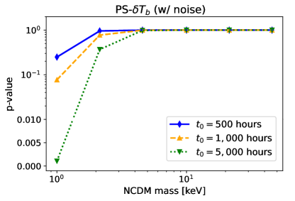
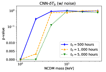
Figure 9: Difference in $p$-values of the KS test due to the observation time $t_{0}=$500 (blue solid), 1,000 (orange dashed), and 5,000 (green dotted) hours for the power spectrum (left panel) and our CNN (right panel). For the same integration time, CNN shows better performance than the power spectrum. For example, our CNN can distinguish dark matter models for $m_{\rm DM}=$ 1 keV with $t_{0}=500$ hours and $m_{\rm DM}=$ 2.1 keV with $t_{0}=1,000$ hours with $p$-value $<0.01$ while the power spectrum cannot distinguish dark matter models $m_{\rm DM}=$ 1 keV even with $t_{0}=5,000$ hours.

In this subsection, we introduce a more realistic situation by considering the system noise, particularly assuming the SKA-MID survey.

In order to generate the mock data including the system temperature noise, we first generate the 3-dimensional map of the random Gaussian white noise spectrum. The size of the noise map is $100\ h^{-1}\mathrm{Mpc}$ on a side and we define the $1024^{3}$ grid. The fluctuation of the noise in this map follows the Gaussian distribution of ${\cal N}(0,\sqrt{P_{\rm noise}})$ And then, we add this noise map to the simulation box after STEP 1 in Section II.4. Finally, we generate images following the same procedures in Section II.4.

The power spectrum of this Gaussian noise $P_{\rm noise}(\mbox{\boldmath${k}$})$ is written as Geil2010

$$P_{\rm noise}(\mbox{\boldmath${k}$})=\frac{T^{2}_{\rm sys}}{t_{0}}\frac{D^{2}}{n_{\rm b}(k_{\perp}D/2\pi,\nu)}\frac{c(1+z)^{2}}{\nu_{0}H(z)}\left(\frac{\lambda^{2}}{A_{\rm e}}\right)^{2},$$ (19)

where $T_{\rm sys}=70$ K is the system temperature, $t_{0}$ is the total integration time, $D\sim 4400$ $h^{-1}$Mpc is the comoving distance to the source at $z=3.0$, $\lambda=c(1+z)/\nu_{0}$ is the observed wavelength, $A_{e}=140\ \mathrm{m}^{2}$ is the effective area of the telescope. $n_{b}(U,\nu)$ is the number density of the baseline given by

$$n_{b}(k_{\perp}D/2\pi,\nu)= C_{b}\int^{r_{\rm max}}_{0}dr\ 2\pi rn_{a}(r)$$

$$\times\int^{2\pi}_{0}d\phi\ n_{a}(|\mbox{\boldmath${r}$}-\lambda\mbox{\boldmath${k}$}_{\perp}D/2\pi|),$$ (20)

where $k_{\perp}$ is the component of the wavevector ${k}$ perpendicular to the line of sight, $\nu$ is the observed frequency, $r_{\rm max}=100$ km is the maximum distance between the center of antennas and another antenna. $n_{a}$ is the number density of the antenna given by

$$n_{a}(r)=\begin{cases}n_{c}&(r\leq r_{c})\\ n_{c}\left(r_{c}/r\right)^{2}&(r_{c}<r<r_{\rm max})\\ 0&(r\geq r_{\rm max})\ ,\end{cases}$$ (21)

as a function of the distance $r$ from the center of antennas, where $n_{c}=N_{a}/(\pi r^{2}_{c}+\ln{(r_{\rm max}/r_{c})})$ is the antenna number density of the core, $r_{c}=0.5$ km is the radius of the core, $N_{a}=254$ is the number of the antenna, and $C_{b}$ is the normalization factor defined by $(1/2\pi)\int k_{\perp}D^{2}n_{\rm b}(k_{\perp}D/2\pi)dk_{\perp}=N_{\rm a}(N_{\rm a}-1)/2$. In these calculations, we use the value of parameters given in Villaescusa-Navarro2015 .

We use images including the noise for training and testing our CNN. We assume the integration time $t_{0}=$500 hours and hours 1,000 following Villaescusa-Navarro2015 , and in addition, we assume $t_{0}=$ 5,000 hours to test the effect of integration time in Eq. (19), where $t_{0}=1,000$ is often quoted in the literature (e.g., Villaescusa-Navarro2015, ; Crocce2006, ; Pritchard2015, ).

As we can see in Fig. 9, the PS analysis can distinguish dark matter models for $m_{\rm DM}=$ 1 keV if we have enough integration time, $t_{0}=5,000$ hours at more than 3 $\sigma$, but for observation time $t_{0}=1,000$ hours, we cannot discriminate the dark matter model of $m_{\rm DM}=1$ keV from the CDM. Even in the case with the noise, the CNN analysis is again superior to the PS analysis. We see that the CNN can distinguish dark matter models for $m_{\rm DM}=$ 1 keV even if the integration time is $t_{0}=500$ hours and for $m_{\rm DM}=$ 2.1 keV NCDM with $t_{0}=1,000$ hours. Although the system noise in $\delta T_{b}$ images degrades the performance of both PS and CNN analyses, CNN still provides better performance than the power spectrum. The information about the dark matter particle mass for $m_{\rm DM}\leq 2.1$ keV, which cannot be captured by the power spectrum still remains behind the system noise of SKA-MID, and the CNN can successfully extract it.

In addition, we discuss the effect of the different astrophysical models under the existence of the system noise of SKA. The classification with our CNN for $m_{\rm DM}>10$ keV is largely disturbed by the different astrophysical models as shown in Fig. 6. However, with the observation time $t_{0}=1,000$ hours, the system noise hides the signals for $m_{\rm DM}\geq 4.6$ keV as shown in Fig. 9. Therefore, the difference in the astrophysical model should not be seriously considered given the observational errors in the era of SKA, but it must be the most serious systematic effect in future higher sensitivity observations.

Finally, we consider the effect of the survey area on our results. Our test images covered a $(100\ h^{-1}\mathrm{Mpc})^{2}$ area across three redshift slices, corresponding to about 5 $\mathrm{deg}^{2}$ of sky at redshift $z=3$. To investigate the impact of the survey area, we derive the $p$-values of the KS test for a limited number of test samples. Specifically, we test the effect of using test images from half of the simulation volume, which corresponds to a survey area of 2.5 square degrees. We find that as the survey area increases, the $p$-values decrease for the classification for $m_{\rm DM}\leq 4.6$ keV dark matter models. This suggests that increasing the survey area could improve the accuracy of our dark matter mass constraints.

V Summary

In summary, this paper explores the use of CNN to distinguish between different models of dark matter based on images and power spectra of 21cm brightness temperature distribution. We have shown that the CNN can better distinguish between different masses of the dark matter particle compared to the power spectrum. We conduct a suite of hydrodynamic simulations with different dark matter particle masses and generate the images of dark matter distribution and $\delta T_{b}$ map. In addition, we perform additional three simulations for the CDM model, where the astrophysical models such as self-shielding of HI gas, star formation, and UV background are different from the Fiducial simulation (Nagamine_2021, ). We also injected the system noise from upcoming SKA-MID observation into the $\delta T_{b}$ images to investigate the effect of noise.

Firstly, we compare the analysis of dark matter images and $\delta T_{b}$ images assuming the Fiducial astrophysical model. Our results indicate that the direct observable $\delta T_{b}$ map can be used to constrain the dark matter mass and has comparable classification power to the dark matter image. We then compare the performance of our CNN and the power spectrum, finding that our CNN can distinguish dark matter models for $m_{\rm DM}\leq 10$ keV, while the power spectrum is only able to distinguish models for $m_{\rm DM}\leq 2.1$ keV. Therefore, we confirm that the CNN can extract the information not encoded in the power spectrum, which is expected due to the non-linear evolution of dark matter, which scrambles the Gaussian information at the initial condition, and the nonlinear relation between dark matter and neutral hydrogen.

Secondly, we explore how different astrophysical models affect the analysis using power spectrum and CNN. To do so, we replace the CDM test images for the Fiducial astrophysical model with those for other astrophysical models. We find that the power spectrum analysis can distinguish the dark matter models for $m_{\rm DM}\leq 2.1$,keV from CDM, regardless of the astrophysical model used. However, the CNN analysis can distinguish dark matter models up to $m_{\rm DM}\leq 4.6$ keV. The classification accuracy at $m_{\rm DM}\sim 10$ keV is significantly affected by assuming the wrong astrophysical model.

Thirdly, we investigate the impact of system temperature noise assuming the SKA-MID observation for the $\delta T_{b}$ map on our classification analysis. We find that the noise significantly degrades the classification performance, but our CNN can still distinguish the NCDM model with $m_{\rm DM}<1$ keV from the CDM model with an integration time of $t_{0}=500$ hours. With more integration time of $t_{0}=5000$ hours, this limit can be extended to $m_{\rm DM}<2.1$keV.

Finally, we also investigate the effect of survey area on our analysis. Our simulations correspond to a survey area of 5 deg² at $z=3$, but by scaling the number of test images, we find the probability that the $p$-values for the classification for the $m_{\rm DM}\leq 4.6$ keV dark matter model can be improved.

Our work demonstrates that CNNs have the potential to more effectively constrain the dark matter particle mass than the power spectrum using the $\delta T_{b}$ map, which can be observed by radio observation like SKA. However, practical observations come with their own challenges, such as foreground contamination and the optimal redshift for constraining the dark matter mass. We plan to address these challenges in future work.

Appendix A Property of HI Halo

Model	$\mu$ [$h^{-1}$kpc]	$\sigma$ [$h^{-1}$kpc]	Total Number
Fiducial	66.2	28.2	270,931
Shield	66.2	28.2	270,930
NoSF	66.2	28.2	271,092
FG09	66.2	28.2	270,936
46 keV	66.2	28.2	269,283
21 keV	66.2	28.5	264,444
10 keV	66.2	28.5	245,598
4.6 keV	65.2	31.9	196,314
2.1 keV	61.9	34.6	126,987
1 keV	59.9	36.7	54,755

Table 3: Radial size of dark matter halos and the number of halos for different astrophysical and dark matter models. The first four rows are the CDM with different astrophysical models, and the latter six rows are the NCDM models. The second and third column shows the mean ($\mu$) and standard deviation ($\sigma$) of the virial radius of the halo, and the last column shows the total number of the halo in the simulation box. Different astrophysical or dark matter models do not have a significant effect on the halo size. However, the number of halos is decreased for the light dark matter models.

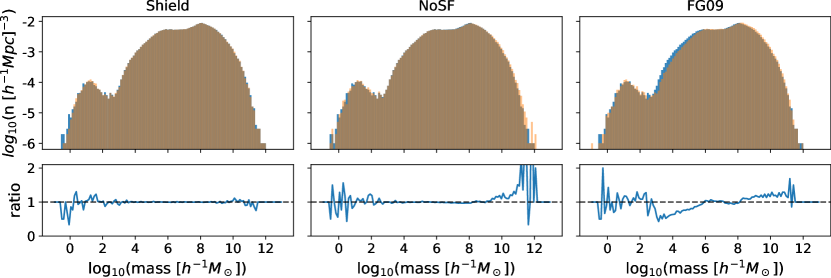
Figure 10: Halo mass function (i.e., the comoving number density of halos as a function of their mass) for Fiducial (blue) and other astrophysical models (orange) in the top panels and the ratio of them in the bottom panels.

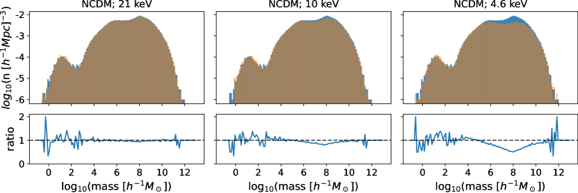
Figure 11: Halo mass function for Fiducial (blue) and other NCDM models (orange) in the top panels and the ratio of them in the bottom panels.

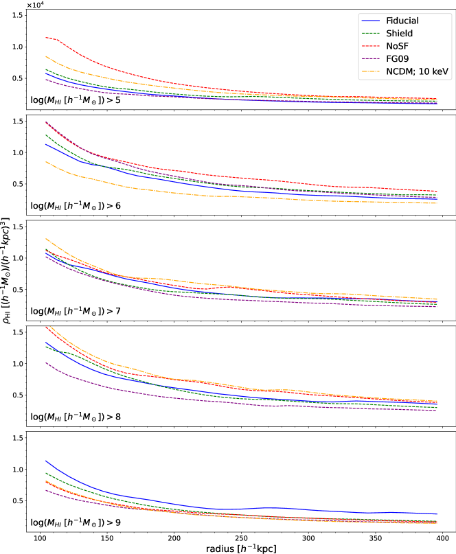
Figure 12: Stacked HI density profile as a function of halo-centric radius. We use up to the 3000th halo counted from the lower end in each mass bin of $\log{(M_{\rm HI}\ [h^{-1}M_{\odot}])}\geq$ 5, 6, 7, 8 and 9 for stacking. Each line corresponds to Fiducial (blue solid), Shield (green dashed), NoSF (red dashed), FG09 (purple dashed), and 10 keV NCDM (orange dash-dot). The lower limit of abscissa corresponds to the pixel size of the images we use.

As we discussed in Fig. 6, a large amount of the test images of CDM is misclassified to the NCDM model if we use the images for different astrophysical models of NoSF or FG09. In this appendix, we try to address how this confusion happens by focusing on the basic quantities of halos. We identify the dark matter halo by using the ROCKSTAR code (rockstar, ) and define the HI halo as the group of the HI gas particles within the virial radius of the dark matter halo.

Table 3 shows the size of the halo which is defined as the virial radius of the dark matter halo and the total number of halos in the simulation box for each astrophysical and dark matter model. For the variant run of the astrophysical model, we always fix the dark matter model to CDM and for the NCDM run, we apply Fiducial astrophysical model. We see that there is no significant relation between the number of halos and the assumption of the astrophysical models, whereas the total number of halos is smaller when the dark matter mass is smaller, especially for $m_{\rm DM}\leq 4.6$ keV. This is because the light dark matter is preventing the clustering on small scales due to its velocity dispersion (see Section II.1) and halos are not formed. On the other hand, the size of the halos is not affected by both the astrophysical models or the dark matter models.

In Fig. 10 and Fig. 11, the panels show the HI mass function in comparison with the Fiducial CDM model. These two figures show the mass function of the astrophysical and NCDM models, respectively. We see that the number of halos of $M_{\rm HI}>10^{9}M_{\odot}/h$ increases in the NoSF and FG09 model compared to the Fiducial model and the halos of $M_{\rm HI}\sim 10^{8}\ h^{-1}M_{\odot}$ decrease for $m_{\rm DM}\leq 10$ keV NCDM models. However, these features do not explain the confusion of the model classification because there are no similarities between the HI halo mass function for the NCDM model and variant astrophysical models.

Then we will see if the halo profile looks similar between the NCDM model and variant astrophysical models. In Fig. 12, the panels show the stacked HI density profile of the halo. To compute the stacked HI density profile, we average the HI mass within the dark matter virial radius over the lowest 3000 halos within each mass bin from $10^{5}$ to $10^{9}h^{-1}M_{\odot}$. The Fiducial (blue solid) and Shield (green dashed) runs have relatively similar profiles. In addition, NoSF (red dashed) and 10 keV NCDM (orange dash-dot) have similar profiles except for halos with $M_{\rm HI}>10^{6}\ h^{-1}M_{\odot}$. Therefore, it is probable that these profiles explain part of the misclassification by our CNN. For FG09 model, its profiles (purple dashed) deviate from Fiducial, especially for massive halos ($M_{\rm HI}>10^{8}\ h^{-1}M_{\odot}$) , but they are also different from 10 keV NCDM profile. As we said in Section IV.2, it is probable that our CNN classification is based not only on features that resemble NCDM, but also on features that are not CDM-like.

References

- (1) A. Boyarsky, M. Drewes, T. Lasserre, S. Mertens, and O. Ruchayskiy, Progress in Particle and Nuclear Physics 104, 1 (2019), 1807.07938.
- (2) A. Alvarez et al., arXiv e-prints , arXiv:2002.01229 (2020), 2002.01229.
- (3) M. Viel, G. D. Becker, J. S. Bolton, and M. G. Haehnelt, Phys. Rev. D88, 043502 (2013), 1306.2314.
- (4) A. Garzilli, A. Magalich, O. Ruchayskiy, and A. Boyarsky, MNRAS502, 2356 (2021), 1912.09397.
- (5) A. Garzilli et al., MNRAS489, 3456 (2019), 1809.06585.
- (6) D. Ribli et al., MNRAS490, 1843 (2019), 1902.03663.
- (7) D. Ribli, B. Á. Pataki, and I. Csabai, Nature Astronomy 3, 93 (2019), 1806.05995.
- (8) S. Pan et al., arXiv e-prints , arXiv:1908.10590 (2019), 1908.10590.
- (9) V. Bonjean, A.&Ap.634, A81 (2020), 1911.10778.
- (10) A. Peel et al., Phys. Rev. D100, 023508 (2019), 1810.11030.
- (11) C. Modi, Y. Feng, and U. Seljak, JCAP2018, 028 (2018), 1805.02247.
- (12) S. J. Tingay et al., Publications of the Astronomical Society of Australia 30, e007 (2013).
- (13) K. Bandura et al., Canadian Hydrogen Intensity Mapping Experiment (CHIME) pathfinder, in Ground-based and Airborne Telescopes V, edited by L. M. Stepp, R. Gilmozzi, and H. J. Hall, , Society of Photo-Optical Instrumentation Engineers (SPIE) Conference Series Vol. 9145, p. 914522, 2014, 1406.2288.
- (14) L. B. Newburgh et al., HIRAX: a probe of dark energy and radio transients, in Ground-based and Airborne Telescopes VI, edited by H. J. Hall, R. Gilmozzi, and H. K. Marshall, , Society of Photo-Optical Instrumentation Engineers (SPIE) Conference Series Vol. 9906, p. 99065X, 2016, 1607.02059.
- (15) M. Santos et al., PoS AASKA14, 019 (2015).
- (16) I. P. Carucci, F. Villaescusa-Navarro, M. Viel, and A. Lapi, JCAP2015, 047 (2015), 1502.06961.
- (17) P. Villanueva-Domingo and F. Villaescusa-Navarro, The Astrophysical Journal 907, 44 (2021).
- (18) Planck Collaboration et al., arXiv e-prints , arXiv:1807.06209 (2018), 1807.06209.
- (19) D. Boyanovsky and J. Wu, Phys. Rev. D83, 043524 (2011), 1008.0992.
- (20) J. Lesgourgues, arXiv e-prints , arXiv:1104.2932 (2011), 1104.2932.
- (21) S. Dodelson and L. M. Widrow, Phys. Rev. Lett. 72, 17 (1994), hep-ph/9303287.
- (22) J. Lesgourgues and T. Tram, JCAP2011, 032 (2011), 1104.2935.
- (23) G. B. Field, Proceedings of the IRE 46, 240 (1958).
- (24) R. Ando, A. J. Nishizawa, I. Shimizu, and K. Nagamine, MNRAS507, 2937 (2021), 2011.13165.
- (25) S. R. Furlanetto, S. P. Oh, and F. H. Briggs, physrep 433, 181 (2006), astro-ph/0608032.
- (26) T. Endo, H. Tashiro, and A. J. Nishizawa, MNRAS499, 587 (2020), 2002.00348.
- (27) M. Crocce, S. Pueblas, and R. Scoccimarro, MNRAS373, 369 (2006), astro-ph/0606505.
- (28) M. Götz and J. Sommer-Larsen, ApSS281, 415 (2002).
- (29) M. Götz and J. Sommer-Larsen, ApSS284, 341 (2003), astro-ph/0210599.
- (30) S. Aoyama et al., Monthly Notices of the Royal Astronomical Society 466, 105 (2016), https://academic.oup.com/mnras/article-pdf/466/1/105/10865208/stw3061.pdf.
- (31) I. Shimizu, K. Todoroki, H. Yajima, and K. Nagamine, Monthly Notices of the Royal Astronomical Society 484, 2632 (2019), https://academic.oup.com/mnras/article-pdf/484/2/2632/27662451/stz098.pdf.
- (32) V. Springel, MNRAS364, 1105 (2005), astro-ph/0505010.
- (33) B. D. Smith et al., Grackle: Chemistry and radiative cooling library for astrophysical simulations, Astrophysics Source Code Library, record ascl:1612.020, 2016, 1612.020.
- (34) J. hoon Kim et al., The Astrophysical Journal Supplement Series 210, 14 (2014).
- (35) J. hoon Kim et al., The Astrophysical Journal 833, 202 (2016).
- (36) F. Haardt and P. Madau, The Astrophysical Journal 746, 125 (2012).
- (37) C.-A. Faucher-Giguère, A. Lidz, M. Zaldarriaga, and L. Hernquist, The Astrophysical Journal 703, 1416 (2009).
- (38) K. Nagamine et al., Astrophys. J. 914, 66 (2021), 2007.14253.
- (39) J. J. Monaghan and J. C. Lattanzio, A.&Ap.149, 135 (1985).
- (40) R. H. Lupton, J. E. Gunn, and A. S. Szalay, AJ118, 1406 (1999), astro-ph/9903081.
- (41) A. Paszke et al., Pytorch: An imperative style, high-performance deep learning library, in Advances in Neural Information Processing Systems 32, edited by H. Wallach et al., pp. 8024–8035, Curran Associates, Inc., 2019.
- (42) S. Han, J. Pool, J. Tran, and W. J. Dally, arXiv e-prints , arXiv:1506.02626 (2015), 1506.02626.
- (43) K. He, X. Zhang, S. Ren, and J. Sun, arXiv e-prints , arXiv:1512.03385 (2015), 1512.03385.
- (44) S. Ioffe and C. Szegedy, arXiv e-prints , arXiv:1502.03167 (2015), 1502.03167.
- (45) A. F. Agarap, arXiv e-prints , arXiv:1803.08375 (2018), 1803.08375.
- (46) S. J. Reddi, S. Kale, and S. Kumar, arXiv e-prints , arXiv:1904.09237 (2019), 1904.09237.
- (47) K. A. L., G. Ist. Ital. Attuari 4, 83 (1933).
- (48) N. V. Smirnov, Bulletin Moscow University 2, 3 (1939).
- (49) P. Virtanen et al., Nature Methods 17, 261 (2020).
- (50) P. M. Geil, B. M. Gaensler, and J. S. B. Wyithe, MNRAS418, 516 (2011), 1011.2321.
- (51) F. Villaescusa-Navarro et al., JCAP2015, 034 (2015), 1410.7393.
- (52) J. Pritchard et al., Cosmology from EoR/Cosmic Dawn with the SKA, in Advancing Astrophysics with the Square Kilometre Array (AASKA14), p. 12, 2015, 1501.04291.
- (53) P. S. Behroozi, R. H. Wechsler, and H.-Y. Wu, Astrophys. J. 762, 109 (2013), 1110.4372.