Time-Domain Moment Matching for Second-Order Systems

Abstract

This paper studies a structure-preserving model reduction problem for large-scale second-order dynamical systems via the framework of time-domain moment matching. The moments of a second-order system are interpreted as the solutions of second-order Sylvester equations, which leads to families of parameterized second-order reduced models that match the moments of an original second-order system at selected interpolation points. Based on this, a two-sided moment matching problem is addressed, providing a unique second-order reduced system that match two distinct sets interpolation points. Furthermore, we also construct the reduced second-order systems that matches the moments of both zero and first order derivative of the original second-order system. Finally, the Loewner framework is extended to the second-order systems, where two parameterized families of models are presented that retain the second-order structure and interpolate sets of tangential data.

I Introduction

Second-order dynamical systems are commonly used to capture the behavior of various physical systems, including electrical circuits, power systems, mechanical systems, see e.g., [1, 2, 3, 4, 5]. The dynamics of a linear time-invariant second-order system is described by

$$\bm{\Sigma}:\begin{cases}M\ddot{x}(t)+D\dot{x}(t)+Kx(t)&=Bu(t),\\ C_{1}\dot{x}(t)+C_{0}x(t)&=y(t),\end{cases}$$ (1)

where $M,D,K\in\mathbb{R}^{n\times n}$ are commonly referred to as the mass, damping, and stiffness matrices in mechanical systems. $B\in\mathbb{R}^{n\times p}$ is the input matrix of external forces, and $C_{0},C_{1}\in\mathbb{R}^{q\times n}$ are the output matrices for positions and velocities. The transfer function of the system $\bm{\Sigma}$ is given by

$$W(s)=(C_{1}s+C_{0})(Ms^{2}+Ds+K)^{-1}B.$$

In real applications, the model description (1) often has a high dimension $n$, which requires a large amount of computational resources and thus hinders simulation, prediction, and control of these systems. Therefore, model reduction techniques for large-scale second-order dynamical systems has been paid increasing attention, and reduced order models are indispensable for efficient analysis and optimization of these structured systems.

The essential problem in model reduction of second-order systems is to preserve the second-order structure, allowing for a physical interpretation of the resulting reduced model. However, achieving this preservation is not necessarily straightforward. Although a second-order system (1) can be rewritten in the first-order form, with state vector $[x(t)^{\top}\ \dot{x}(t)^{\top}]^{\top}$, which can be reduced via first-order reduction methods, the reduced-order models generally lose the second-order structure. To cope with this structure-preserving problem, second-order balancing approaches have been proposed in e.g., [6, 7, 8, 9, 10]. The so-called position and velocity Gramians are defined as the diagonal blocks in the Gramian matrices of the first-order representation. Then, balanced truncation can be performed based on different pairs of position and velocity Gramians. However, unlike the balanced truncation in the first-order case, these methods can hardly preserve stability and provide a global error bound. A port-Hamiltonian approach in [11], in contrast, reduces a second-order system via a generalized Hamiltonian framework and preserves the Hamiltonian structure and stability. Recently, a positive real balanced truncation method is presented in [12], which guarantees stability and passivity of reduced second-order model. The model reduction problem in [13, 14] is tackled by optimization approaches, where reduced systems are constructed as the optimal solution of an $H_{2}$-optimization problem subject to certain structural constraint. In [15, 16, 17], a clustering-based framework is considered to simplify the structure of second-order network systems, and the scheme is based on identifying and aggregating nodal states that have similar responses to external input signals.

Moment matching techniques provide efficient tools for model reduction of dynamical systems, see [18, 19, 20, 21, 22] for an extensive overview for first-order systems. By using the projection matrices generated in the Krylov subspace, reduced models are constructed to match the original system at selected interpolation points in the complex plane. Recent extensions to second-order systems are found in e.g., [23, 24, 25, 26, 27], in which the second-order Krylov subspace is introduced to preserve the second-order structure.

A time-domain approach to moment matching has been presented in [28, 21], where the moments of a system are characterized by the unique solutions of Sylvester equations. It is shown that there is a one-to-one relation between the moments and the steady-state response, which is obtained by interconnecting the system with a signal generator interpreting a set of interpolation points. This time-domain approach has been further developed in e.g., [29, 30, 31] for port-Hamiltonian systems and two-sided moment matching problem.

The current paper extends the time-domain moment matching approach to linear second-order systems in (1). Particularly, we represent the moments of $W(s)$ at a set of interpolation points by the unique solution of a second-order Sylvester equation. Thereby, a family of parameterized reduced models in the second-order form is constructed, based on which, we further analyze reduced models that preserve stability and passivity. The another contribution is the two-sided moment matching approach, with which the reduced second-order model matches the moments of $W(s)$ at two distinct sets of interpolation points. Furthermore, we also study the problem of time-domain moment matching for the first-order derivative of the transfer function of the system (1), denoted by $W^{\prime}(s)$. These moments are shown to have a one-to-one relation with the steady-state response of the system composed of the state-space representation of $W^{\prime}(s)$ and two dual signal generators in a cascade form. We present a reduced-order model that achieves moment matching at both zero and first-order derivatives of $W(s)$. Finally, the Loewner framework is extended to the second-order systems, where we present two families of parameterized systems that not only match given sets of right and left tangential data but also possess the second-order structure.

Given a set of right tangential interpolation data, we present two approaches in the Loewner framework to establish a second-order model that interpolates the data.

The paper is organized as follows. In Section II, we present preliminary results regarding time-domain moment matching for linear systems. In Section III, the the moments of a second-order system are characterized with second-order Sylvester equations, and the time-domain moment matching approach for second-order systems is presented. The moment matching problems pertaining two-sided moment matching, pole placement, and first-order derivatives are discussed in Section IV. In Section V, the second-order Loewner framework is presented, and finally, concluding remarks are made in Section VII.

Notation: The symbol $\mathbb{R}$ and $\mathbb{C}$ denotes the sets of real and complex numbers, respectively, and $\mathbb{C}^{-}$ and $\mathbb{C}^{0}$ are the set of complex numbers with negative real part and zero real part, respectively. $\emptyset$ denotes the empty set, and $\mathds{1}_{n\times m}$ represents a matrix with all elements equal to $1$. For a complex matrix $A\in\mathbb{C}^{n\times m}$, $A^{*}\in\mathbb{C}^{m\times n}$ denotes the conjugate transpose of $A$. Moreover, $\sigma(A)$ represents the set of the eigenvalues of $A$, and $\det(A)$ represents the determinant of $A$.

II Preliminaries

In this section we briefly recall the notion of time-domain moment matching a stable LTI system of order one, see e.g., [32, 33].

II-A Time-Domain Moment Matching for Linear Systems

Consider a single input-single output (SISO) linear time-invariant (LTI) minimal system

$$\begin{split}&\Sigma:\;\;\dot{x}=Ax+Bu,\quad y=Cx,\end{split}$$ (2)

with the state $x\in\mathbb{R}^{n}$, the input $u\in\mathbb{R}$ and the output $y\in\mathbb{R}$. The transfer function of (2) is

$$K(s)=C(sI-A)^{-1}B,\quad K:\mathbb{C}\to\mathbb{C}.$$ (3)

Assume that (2) is a minimal realization of the transfer function $K(s)$. The moments of (3) are defined as follows.

Definition 1.

[34, 32] The $k$-moment of system (2) with the transfer function $K$ as in (3), at $s_{1}\in\mathbb{R}$ is defined by $\eta_{k}(s_{1})={(-1)^{k}}/{k!}\left[{\operatorname{d\!}^{k}K(s)}/{\operatorname{d\!}s^{k}}\right]_{s=s_{1}}\in\mathbb{R}.$

For the sake of clarity, without loss of generality, throughout the rest of this section, we consider real quantities.
Picking the points $s_{1},\dots,s_{\nu}\in\mathbb{R}$ let the $S\in\mathbb{R}^{\nu\times\nu}$, with the spectrum $\sigma(S)=\{s_{1},\dots,s_{\nu}\}$. Let $L=[1\ \dots\ 1]\in\mathbb{R}^{1\times\nu}$, such that the pair $(L,S)$ is observable. Denote by $\Pi\in\mathbb{R}^{n\times\nu}$ be the solution of the Sylvester equation

$$A\Pi+BL=\Pi S.$$ (4)

Furthermore, since the system is minimal, assuming that $\sigma(A)\cap\sigma(S)=\emptyset$, then $\Pi$ is the unique solution of the equation (4) and ${\rm rank}\ \Pi=\nu$, see e.g. [35]. Then, the moments of (2) are characterised as follows

Proposition 1.

[32] The moments of system (2) at the interpolation points $\{s_{1},s_{2},...,s_{\ell}\}=\sigma(S)$ are in one-to-one relation with the elements of the matrix $C\Pi$.

The following proposition gives necessary and sufficient conditions for a low-order system to achieve moment matching.

Proposition 2.

[32] Consider the LTI system

$$\begin{split}&\dot{\xi}=F\xi+Gu,\quad\psi=H\xi,\end{split}$$

with $F\in\mathbb{R}^{\nu\times\nu},\ G\in\mathbb{R}^{\nu}$ and $H\in\mathbb{R}^{p\times\nu}$, and the corresponding transfer function

$$K_{G}(s)=H(sI-F)^{-1}G.$$

Fix $S\in\mathbb{R}^{\nu\times\nu}$ and $L\in\mathbb{R}^{1\times\nu}$, such that the pair $(L,S)$ is observable and $\sigma(S)\cap\sigma(A)=\emptyset$. Furthermore, assume that $\sigma(F)\cap\sigma(S)=\emptyset$. The reduced system (2) matches the moments of (2) at $\sigma(S)$ if and only if

$$HP=C\Pi,$$

where the invertible matrix $P\in\mathbb{R}^{\nu\times\nu}$ is the unique solution of the Sylvester equation $FP+GL=PS.$

We are now ready to present a family of $\nu$ reduced order models parameterized in $G$ that match $\nu$ moments of the given system (2). The reduced system

$$\Sigma_{G}:\,\dot{\xi}=(S-GL)\xi+Gu,\quad\psi=C\Pi\xi,$$ (5)

with the transfer function

$$K_{G}(s)=C\Pi(sI-S+GL)^{-1}G,$$ (6)

describes a family of $\nu$ order models that achieve moment matching at $\sigma(S)$ fixed, satisfying the properties

1. $\Sigma_{G}$ is parameterized in $G\in\mathbb{R}^{\nu}$,

2. $\sigma(S-GL)\cap\sigma(S)=\emptyset$.

II-B Time-Domain Moment Matching for MIMO Systems

The results can be directly extended to the MIMO case, see, e.g., [33] for more details. Consider a MIMO system (2), with input $u(t)\in\mathbb{R}^{m}$, output $y(t)\in\mathbb{R}^{p}$ and the transfer function $K(s)\in\mathbb{C}^{p\times m}$. Let $S\in\mathbb{C}^{\nu\times\nu}$ and $L=[l_{1}\ l_{2}\ ...\ l_{\nu}]\in\mathbb{C}^{m\times\nu}$, $l_{i}\in\mathbb{C}^{m}$, $i=1,...,\nu$, be such that the pair $(L,S)$ is observable. Let $\Pi\in\mathbb{C}^{n\times\nu}$ be the unique solution of the Sylvester equation (4). Then the moments $\eta(s_{i})=K(s_{i})l_{i}$, $\eta(s_{i})\in\mathbb{C}^{p}$, $i=1,...,\nu$ of at $\{s_{1},...,s_{\nu}\}=\sigma(S)$ are in one-to-one relation with $C\Pi$. The model reduction problem for MIMO systems boils down to finding a $\nu$-th order model described by the equations (2), with the transfer function $K_{G}$ as in (2), $G\in\mathbb{R}^{\nu\times m}$ which satisfies the right tangetial interpolation conditions [36]

$$K(s_{i})l_{i}=\widehat{K}(s_{i})l_{i},\ i=1,...,\nu.$$

It immediately follows that a family of reduced order MIMO models that achieve moment matching in the sense of satisfying the tangential interpolation conditions is given by $\Sigma_{G}$ described by the equation (5).

III Moments and Moment Matching of Second-order System

III-A Moments of Second-Order Systems

In this section, we characterize the moments of the second-order system $\bm{\Sigma}$ in (1) at a set of interpolation points, which is different from the poles of $\bm{\Sigma}$, defined as follows.

$$\Omega:=\{s\in\mathbb{C}\mid\det(Ms^{2}+Ds+K)=0\},$$ (7)

with $|\Omega|=2n$.

Following [18, 21], the moments of second-order systems are defined as follows.

Definition 2.

Let $s_{\star}\in\mathbb{C}$ such that $s_{\star}\notin\Omega$. The 0-moment of $W(s)$ at $s_{\star}\in\mathbb{C}$ is the complex matrix

$$\eta_{0}(s_{\star})=W(s_{\star})=(C_{1}s_{\star}+C_{0})(Ms_{\star}^{2}+Ds_{\star}+K)^{-1}B,$$

and the $k$-moment at $s_{\star}\in\mathbb{C}$ is defined by

$$\eta_{k}(s_{\star})=\frac{(-1)^{k}}{k!}\left[\frac{\operatorname{d\!}^{k}}{\operatorname{d\!}s^{k}}W(s)\right]_{s=s_{\star}},\ k\geq 1\ \text{and integer}.$$ (8)

Note that the 0-moment of $W(s)$ at $s_{\star}$ can be written as $\eta_{0}(s_{\star})=C_{0}\Pi+C_{1}\Pi s_{\star}$, where $\Pi$ is the unique solution of the matrix equation

$$M\Pi s_{\star}^{2}+D\Pi s_{\star}+K\Pi=B.$$

Then, the following lemma is obtained for moments at distinct interpolation points.

Lemma 1.

Let

$$S =\mathrm{diag}(s_{1},s_{2},\cdots,s_{\nu}),\ \text{and}\ L=\begin{bmatrix}l_{1}&...&l_{\nu}\end{bmatrix},$$

$$Q =\mathrm{diag}(s_{\nu+1},s_{\nu+1},\cdots,s_{2\nu}),\ \text{and}\ R=\begin{bmatrix}r_{1}^{*}&...&r_{\nu}^{*}\end{bmatrix}^{*},$$

where $s_{i}\in\mathbb{C}\setminus\Omega$, $\forall i=1,2,\cdots,2\nu$, $l_{i}\in\mathbb{C}^{p}$, and $r_{i}\in\mathbb{C}^{1\times q}$, $i=1,2,...,\nu$. If the pair $(L,S)$ is observable, and $(Q,R)$ is controllable. Then, the 0-moments $\eta_{0}(s_{i})$ satisfy the following relations

$$\begin{bmatrix}\eta_{0}(s_{1})&\eta_{0}(s_{2})&\cdots&\eta_{0}(s_{\nu})\end{bmatrix} =C_{0}\Pi+C_{1}\Pi S,$$

$$\begin{bmatrix}\eta_{0}(s_{\nu+1})&\eta_{0}(s_{\nu+2})&\cdots&\eta_{0}(s_{2\nu})\end{bmatrix} =\Upsilon B,$$

where $\Pi$, $\Upsilon\in\mathbb{C}^{n\times\nu}$ satisfy the following second-order Sylvester equations

$$M\Pi S^{2}+D\Pi S+K\Pi =BL,$$ (9)

$$Q^{2}\Upsilon M+Q\Upsilon D+\Upsilon K =RC_{0}+QRC_{1}.$$ (10)

Proof.

Let $\Pi=\left[\Pi_{1},\Pi_{2},\cdots,\Pi_{\nu}\right]\in\mathbb{C}^{n\times\nu}$ with $\Pi_{i}\in\mathbb{C}^{n}$. Then, the matrix equation (9) is written as

$$M\Pi_{i}s_{i}^{2}+D\Pi_{i}s_{i}+K\Pi_{i}=Bl_{i},\ \forall i=1,2,\cdots,\nu.$$

It leads to

$$\Pi_{i}=(Ms_{i}^{2}+Ds_{i}+K)^{-1}Bl_{i},$$

Thus, $\eta_{0}(s_{i})=C_{0}\Pi_{i}+C_{1}\Pi_{i}s_{i}$ for all $i=1,2,\cdots,\nu$, which gives the result.

Analogously, we denote $\Upsilon^{*}:=[\Upsilon_{1}^{*},\Upsilon_{1}^{*},\cdots,\Upsilon_{\nu}^{*}]$ with $\Upsilon_{i}\in\mathbb{C}^{1\times n}$. Then, (10) is equivalent to

$$\Upsilon_{i}Ms_{\nu+i}^{2}+\Upsilon_{i}Ds_{\nu+i}+\Upsilon_{i}K=r_{i}^{*}C_{0}+r_{i}^{*}C_{1}s_{\nu+i},$$

for all $i=1,2,\cdots,\nu$. Thus, we obtain

$$\Upsilon_{i}=(r_{i}^{*}C_{0}+r_{i}^{*}C_{1}s_{\nu+i})(Ms_{i+\nu}^{2}+Ds_{i+\nu}+K)^{-1},$$

which gives the 0-moments $\eta_{0}(s_{\nu+1})$, $\cdots$, $\eta_{0}(s_{2\nu})$. ∎

Furthermore, the following lemma provides the characterization of the moments at a single interpolation point with higher order derivatives.

Lemma 2.

Consider the second-order system in (1) and $s_{\star},z_{\star}\in\mathbb{C}\setminus\Omega$. Let the matrices $S\in\mathbb{C}^{(\nu+1)\times(\nu+1)}$, $L\in\mathbb{R}^{p\times(\nu+1)}$ and $Q\in\mathbb{R}^{(\nu+1)\times(\nu+1)}$, $R\in\mathbb{R}^{(\nu+1)\times q}$ be such that the pair $(L,S)$ is observable, and the pair $(Q,R)$ is controllable, respectively. Suppose $S$ and $Q$ are non-derogatory such that

$$\det(sI-S)=(s-s_{\star})^{\nu+1},\ \det(sI-Q)=(s-z_{\star})^{\nu+1}.$$

Then the following statements hold.

1. There exists a one-to-one relation between the moments $\eta_{0}(s_{\star})$, $\eta_{1}(s_{\star})$, $\cdots$, $\eta_{\nu}(s_{\star})$ and and the matrix $C_{0}\Pi+C_{1}\Pi S$, where $\Pi$ satisfies

   $$M\Pi S^{2}+D\Pi S+K\Pi=BL.$$ (11)

2. There exists a one-to-one relation between the moments $\eta_{0}(z_{\star})$, $\eta_{1}(z_{\star})$, $\cdots$, $\eta_{\nu}(z_{\star})$ and and the matrix $\Upsilon B$, where $\Upsilon$ satisfies

   $$Q^{2}\Upsilon M+Q\Upsilon D+\Upsilon K=RC_{0}+QRC_{1}.$$ (12)

Proof.

For simplicity, let $\mathscr{F}(s)=(Ms^{2}+Ds+K)^{-1}$. Due to $\mathscr{F}(s)^{-1}\mathscr{F}(s)=I$, we have

$$\frac{d}{ds}\left[\mathscr{F}(s)^{-1}\mathscr{F}(s)\right]=\frac{d}{ds}\mathscr{F}(s)^{-1}\mathscr{F}(s)+\mathscr{F}(s)^{-1}\frac{d}{ds}\mathscr{F}(s)=0.$$

Thus, we obtain the first-order derivate of $\mathscr{F}(s)$ as

$$\frac{d}{ds}\mathscr{F}(s)=-\mathscr{F}(s)\frac{d}{ds}\mathscr{F}(s)^{-1}\mathscr{F}(s),$$

The above equation is important, as it facilitates the calculation of the second order derivative of $\mathscr{F}(s)$:

$$\begin{split}\frac{d^{2}}{ds^{2}}\mathscr{F}(s)=&-\frac{d}{ds}\left[\mathscr{F}(s)\frac{d}{ds}\mathscr{F}(s)^{-1}\mathscr{F}(s)\right]\\ =&2\mathscr{F}(s)\frac{d}{ds}\mathscr{F}(s)^{-1}\mathscr{F}(s)\frac{d}{ds}\mathscr{F}(s)^{-1}\mathscr{F}(s)\\ &-\mathscr{F}(s)\frac{d^{2}}{ds^{2}}\mathscr{F}(s)^{-1}\mathscr{F}(s)\\ =&-2\mathscr{F}(s)\frac{d}{ds}\mathscr{F}(s)^{-1}\frac{d}{ds}\mathscr{F}(s)\\ &-\mathscr{F}(s)\frac{d^{2}}{ds^{2}}\mathscr{F}(s)^{-1}\mathscr{F}(s),\end{split}$$

where

$$\frac{d}{ds}\mathscr{F}(s)^{-1}=2Ms+D,\ \text{and}\ \frac{d^{2}}{ds^{2}}\mathscr{F}(s)^{-1}=2M.$$ (13)

More generally, the $k$-th order ($k\geq 2$) of $\mathscr{F}(s)$ derivative can be proven by induction. The result is given by

$$\begin{split}\frac{d^{k}}{ds^{k}}\mathscr{F}(s)=&-k\mathscr{F}(s)\frac{d}{ds}\mathscr{F}(s)^{-1}\frac{d^{k-1}}{ds^{k-1}}\mathscr{F}(s)\\ &-\frac{k(k-1)}{2}\mathscr{F}(s)\frac{d^{2}}{ds^{2}}\mathscr{F}(s)^{-1}\frac{d^{k-2}}{ds^{k-2}}\mathscr{F}(s).\end{split}$$ (14)

We start proving the first statement. Let $\Pi=\left[\Pi_{0},\Pi_{1},\cdots,\Pi_{\nu}\right]\in\mathbb{C}^{n\times(\nu+1)}$ with $\Pi_{0}=(Ms_{\star}^{2}+Ds_{\star}+K)^{-1}Bl_{0}$ and

$$\Pi_{k}:=\frac{1}{k!}\left[\left.\frac{d^{k}}{ds^{k}}\mathscr{F}(s)\right\rvert_{s=s_{\star}}\right]Bl_{0},\ k=1,2,\cdots,\nu,$$ (15)

where $l_{0}\in\mathbb{C}^{p}$. Note that pre-multiplying $\frac{1}{k!}$ to (14) yields

$$\begin{split}\frac{1}{k!}\frac{d^{k}}{ds^{k}}\mathscr{F}(s)=-\mathscr{F}(s)\frac{d}{ds}\mathscr{F}(s)^{-1}\left[\frac{1}{(k-1)!}\frac{d^{k-1}}{ds^{k-1}}\mathscr{F}(s)\right]\\ -\frac{1}{2}\mathscr{F}(s)\frac{d^{2}}{ds^{2}}\mathscr{F}(s)^{-1}\left[\frac{1}{(k-2)!}\frac{d^{k-2}}{ds^{k-2}}\mathscr{F}(s)\right],\end{split}$$

which implies

$$\begin{split}\left(Ms_{\star}^{2}+Ds_{\star}+K\right){\Pi}_{0}=&Bl_{0},\\ \left(Ms_{\star}^{2}+Ds_{\star}+K\right)\Pi_{1}=&-\left(2Ms_{\star}+D\right)\Pi_{0},\\ \left(Ms_{\star}^{2}+Ds_{\star}+K\right)\Pi_{2}=&-\left(2Ms_{\star}+D\right)\Pi_{1}-M\Pi_{0},\\ \vdots\\ \left(Ms_{\star}^{2}+Ds_{\star}+K\right)\Pi_{\nu}=&-\left(2Ms_{\star}+D\right)\Pi_{\nu-1}-M\Pi_{\nu-2}.\end{split}$$

Therefore, we obtain a series of second-order Sylvester equations as follows.

$$\begin{split}M\Pi_{0}s_{\star}^{2}+D\Pi_{0}s_{\star}+K\Pi_{0}=&Bl_{0},\\ M(\Pi_{1}s_{\star}^{2}+2\Pi_{0}s_{\star})+D(\Pi_{1}s_{\star}+\Pi_{0})+K\Pi_{1}=&0,\\ M(\Pi_{2}s_{\star}^{2}+2\Pi_{1}s_{\star}+\Pi_{0})+D(\Pi_{2}s_{\star}+\Pi_{1})+K\Pi_{2}=&0,\\ \vdots&\\ M(\Pi_{\nu}s_{\star}^{2}+2\Pi_{\nu-1}s_{\star}+\Pi_{\nu-2})\hskip 96.0pt&\\ +D(\Pi_{\nu}s_{\star}+\Pi_{\nu-1})+K\Pi_{\nu}=&0,\end{split}$$

The above equations can be written in a compact form:

$$M\Pi\bar{S}^{2}+D\Pi\bar{S}+K\Pi=B\bar{L},$$ (16)

where $\bar{L}=\begin{bmatrix}l_{0}&0&...&0\end{bmatrix}\in\mathbb{C}^{p\times(\nu+1)}$ and

$$\bar{S}=\begin{bmatrix}s_{\star}&1&0&\cdots&0\\ 0&s_{\star}&1&\cdots&0\\ \vdots&\vdots&\ddots&\ddots&\vdots\\ 0&\cdots&0&s_{\star}&1\\ 0&\cdots&\cdots&0&s_{\star}\\ \end{bmatrix}\in\mathbb{C}^{(\nu+1)\times(\nu+1)}.$$

Next, the moments at $\sigma(S)$ are characterized. The 0-moment is obtained directly as

$$\eta_{0}(s_{\star})=(C_{0}+C_{1}s_{\star})\mathscr{F}(s_{\star})B=C_{0}\Pi_{0}+C_{1}\Pi_{0}s_{\star}.$$

Furthermore, we observe that

$$\begin{split}&\frac{d^{k}}{ds^{k}}\left[(C_{0}+C_{1}s)\mathscr{F}(s)\right]\\ =&C_{1}\frac{d^{k-1}}{ds^{k-1}}\mathscr{F}(s)+\frac{d^{k-1}}{ds^{k-1}}\left[(C_{0}+C_{1}s)\frac{d}{ds}\mathscr{F}(s)\right]\\ =&2C_{1}\frac{d^{k-1}}{ds^{k-1}}\mathscr{F}(s)+\frac{d^{k-2}}{ds^{k-2}}\left[(C_{0}+C_{1}s)\frac{d^{2}}{ds^{2}}\mathscr{F}(s)\right]\\ =&\cdots=kC_{1}\frac{d^{k-1}}{ds^{k-1}}\mathscr{F}(s)+(C_{0}+C_{1}s)\frac{d^{k}}{ds^{k}}\mathscr{F}(s).\end{split}$$ (17)

Thus, by the definition of the $k$-moment in (8), we have

$$\begin{split}\eta_{k}(s_{\star})=&\frac{(-1)^{k}}{k!}\left.\frac{d^{k}}{ds^{k}}\left[(C_{0}+C_{1}s)\mathscr{F}(s)\right]B\right\rvert_{s=s_{\star}}\\ =&\frac{(-1)^{k}}{(k-1)!}\left.C_{1}\frac{d^{k-1}}{ds^{k-1}}\mathscr{F}(s)B\right\rvert_{s=s_{\star}}\\ &+\frac{(-1)^{k}}{k!}(C_{0}+C_{1}s_{\star})\left.\frac{d^{k}}{ds^{k}}\mathscr{F}(s)B\right\rvert_{s=s_{\star}}\\ =&(-1)^{k}\left[C_{1}\Pi_{k-1}+(C_{0}+C_{1}s_{\star})\Pi_{k}\right]\\ =&(-1)^{k}\left[C_{0}\Pi_{k}+C_{1}(\Pi_{k-1}+\Pi_{k}s_{\star})\right],\end{split}$$

for $k=1,2,\cdots,\nu$. Consequently, the following relation holds.

$$\begin{bmatrix}\eta_{0}(s_{\star})&\eta_{1}(s_{\star})&\cdots&\eta_{\nu}(s_{\star})\end{bmatrix}=(C_{0}\Pi+C_{1}\Pi S)\Phi_{\nu},$$

with $\Phi_{\nu}=\mathrm{diag}(1,-1,1,\cdots,(-1)^{\nu}).$ Therefore, there is a one-to-one relation between the moments $\eta_{k}(s_{\star})$ and the entries of the matrix $C_{0}{\Pi}+C_{1}{\Pi}S$.

Notice that the pair $(\bar{L},\bar{S}$ is observable for any $s_{\star}$. For a given pair $(L,S)$ that is observable, there exists a unique invertible matrix $T\in\mathbb{R}^{(\nu+1)\times(\nu+1)}$ such that $\bar{S}=T{S}T^{-1}$ and $\bar{L}=T^{-1}{L}$. Substituting $\bar{S}$ and $\bar{L}$ into (16) yields the Sylvester equation in (11).

Now, we prove the second statement. Before proceeding, we claim that

$$\begin{split}\frac{d^{k}}{ds^{k}}\mathscr{F}(s)=&-k\frac{d^{k-1}}{ds^{k-1}}\mathscr{F}(s)\frac{d}{ds}\mathscr{F}(s)^{-1}\mathscr{F}(s)\\ &-\frac{k(k-1)}{2}\frac{d^{k-2}}{ds^{k-2}}\mathscr{F}(s)\frac{d^{2}}{ds^{2}}\mathscr{F}(s)^{-1}\mathscr{F}(s),\end{split}$$ (18)

where $\frac{d}{ds}\mathscr{F}(s)^{-1}$ and $\frac{d^{2}}{ds^{2}}\mathscr{F}(s)^{-1}$ are defined in (13). The proof is similar to (18). Let $\Upsilon=\left[\Upsilon_{0}^{*},\Upsilon_{1}^{*},\cdots,\Upsilon_{\nu}^{*}\right]^{*}\in\mathbb{C}^{(\nu+1)\times n}$ with $\Upsilon_{0}=(r_{0}^{*}C_{0}+r_{0}^{*}C_{1}z_{\star})(Mz_{\star}^{2}+Dz_{\star}+K)^{-1}$ and

$$\Upsilon_{k}:=\frac{1}{k!}\left[\left.\frac{d^{k}}{ds^{k}}(r_{0}^{*}C_{0}+r_{0}^{*}C_{1}s)\mathscr{F}(s)\right\rvert_{s=z_{\star}}\right],k=1,2,\cdots,\nu,$$

where $r_{0}\in\mathbb{C}^{1\times q}$. Observe that by Definition 2, there is a one-to-one relation between $\Upsilon_{k}$ and the moment $\eta_{k}(z_{\star})$:

$$\eta_{0}(z_{\star})=\Upsilon_{0}B,\ \eta_{k}(z_{\star})=(-1)^{k}\Upsilon_{k}B.$$

For simplicity, we denote

$$\phi_{k}=\frac{1}{k!}\left[\left.\frac{d^{k}}{ds^{k}}\mathscr{F}(s)\right\rvert_{s=z_{\star}}\right].$$

Thus, from (17) and (18), the following equations hold.

$$\Upsilon_{k} =r_{0}^{*}C_{1}\phi_{k-1}+(r_{0}^{*}C_{0}+r_{0}^{*}C_{1}z_{\star})\phi_{k},$$

$$\phi_{k} =-\phi_{k-1}(2Mz_{\star}+D)\mathscr{F}(z_{\star})-\phi_{k-2}M\mathscr{F}(z_{\star}).$$

Combining the above equations, we obtain the relation between $\Upsilon_{k}$, $\Upsilon_{k-1}$ and $\Upsilon_{k-2}$:

$$\Upsilon_{k}\mathscr{F}(z_{\star})^{-1}= \Upsilon_{k}(Mz_{\star}^{2}+Dz_{\star}+K)$$

$$-C_{1}\phi_{k-2}(2Mz_{\star}+D)-C_{1}\phi_{k-3}M$$

$$-(C_{0}+C_{1}z_{\star})\phi_{k-1}(2Mz_{\star}+D)$$

$$-(C_{0}+C_{1}z_{\star})\phi_{k-2}M$$

$$= -\Upsilon_{k-1}(2Mz_{\star}+D)-\Upsilon_{k-2}M.$$

Then, similar to the proof of the first statement, we therefore obtain a second-order Sylvester equation:

$$\bar{Q}^{2}\Upsilon M+\bar{Q}\Upsilon D+\Upsilon K=\bar{R}C_{0}+\bar{Q}\bar{R}C_{1},$$

where $\bar{R}=\begin{bmatrix}r_{0}^{*}&0&...&0\end{bmatrix}^{*}\in\mathbb{C}^{(\nu+1)\times q}$ and

$$\bar{Q}=\begin{bmatrix}z_{\star}&0&0&\cdots&0\\ 1&z_{\star}&0&\cdots&0\\ \vdots&\ddots&\ddots&\ddots&\vdots\\ 0&\cdots&1&z_{\star}&0\\ 0&\cdots&\cdots&1&z_{\star}\\ \end{bmatrix}\in\mathbb{C}^{(\nu+1)\times(\nu+1)}.$$

Since both pairs $(\bar{Q},\bar{R})$ and $(Q,R)$ are controllable, there exists a unique invertible matrix $\tilde{T}$ such that $\bar{Q}=TQT^{-1}$ and $\bar{R}=TR$, which yields (12). ∎

Let us combine the conclusions in Lemma 1 and Lemma 2, which leads to the following result.

Theorem 1.

Consider the second-order system (1) with transfer function $W(s)$. Let the matrices $S\in\mathbb{C}^{\nu\times\nu}$, $L\in\mathbb{R}^{p\times\nu}$ and $Q\in\mathbb{R}^{\nu\times\nu}$, $R\in\mathbb{R}^{\nu\times q}$ be such that the pair $(L,S)$ is observable, and the pair $(Q,R)$ is controllable, respectively. Then, the following statements hold.

1. If $\sigma(S)\cap\Omega=\emptyset$, there is a one-to-one relation between the moments of $W(s)$ at $\sigma(S)$ and the matrix $C_{0}\Pi+C_{1}\Pi S$, where $\Pi\in\mathbb{C}^{n\times\nu}$ is the unique solution of

   $$M\Pi S^{2}+D\Pi S+K\Pi=BL.$$ (19)

2. If $\sigma(Q)\cap\Omega=\emptyset$, there is a one-to-one relation between the moments of $W(s)$ at $\sigma(Q)$ and the matrix $\Upsilon B$, where $\Upsilon\in\mathbb{C}^{\nu\times n}$ is the unique solution of

   $$Q^{2}\Upsilon M+Q\Upsilon D+\Upsilon K=RC_{0}+QRC_{1}.$$ (20)

Proof.

It follows from the results in Lemma 1 and Lemma 2 that the moments moments of $W(s)$ at $\sigma(S)$ and $\sigma(Q)$ are characterized by $C_{0}\Pi+C_{1}\Pi S$ and $\Upsilon B$, respectively, where $\Pi$ and $\Upsilon$ satisfy the second-order Sylvester equations in (19) and (20), respectively. Then, in this proof, we show the solutions of (19) and (20) are unique.

Consider the following first-order Sylvester equations:

$$\begin{bmatrix}0&I\\ -M^{-1}K&-M^{-1}D\end{bmatrix}\tilde{\Pi}+\begin{bmatrix}0\\ M^{-1}B\end{bmatrix}L=\tilde{\Pi}S,$$ (21)

and

$$\tilde{\Upsilon}\begin{bmatrix}0&I\\ -M^{-1}K&-M^{-1}D\end{bmatrix}+R\begin{bmatrix}C_{0}&C_{1}\end{bmatrix}=Q\tilde{\Upsilon},$$ (22)

where $\tilde{\Pi}\in\mathbb{C}^{2n\times\nu}$ and $\tilde{\Upsilon}\in\mathbb{C}^{\nu\times 2n}$. Note that the roots of

$$\left|sI_{2n}-\begin{bmatrix}0&I\\ -M^{-1}K&-M^{-1}D\end{bmatrix}\right|=0$$

coincide with $\Omega$ in (7). Since $\sigma(S)\cap\Omega=\emptyset$ and $\sigma(Q)\cap\Omega=\emptyset$, $\tilde{\Pi}$ and $\tilde{\Upsilon}$ are unique solutions of (21) and (22), respectively.

Furthermore, we show the one-to-one relations between $\tilde{\Pi}$ and $\Pi$ as well as between $\tilde{\Upsilon}$ and $\Upsilon$. Partition $\tilde{\Pi}$ and $\tilde{\Upsilon}$ as

$$\tilde{\Pi}=\begin{bmatrix}\tilde{\Pi}_{a}\\ \tilde{\Pi}_{b}\end{bmatrix},\ \text{with}\ \tilde{\Pi}_{a},\tilde{\Pi}_{b}\in\mathbb{C}^{n\times\nu},$$

$$\tilde{\Upsilon}=\begin{bmatrix}\tilde{\Upsilon}_{a}&\tilde{\Upsilon}_{b}\end{bmatrix},\ \text{with}\ \tilde{\Upsilon}_{a},\tilde{\Upsilon}_{b}\in\mathbb{C}^{\nu\times n},$$

which lead to

$$\tilde{\Pi}_{b} =\tilde{\Pi}_{a}S,$$ (23a)

$$BL =M\tilde{\Pi}_{b}S+D\tilde{\Pi}_{b}+K\tilde{\Pi}_{a},$$ (23b)

and

$$-\tilde{\Upsilon}_{b}M^{-1}K+RC_{0} =Q\tilde{\Upsilon}_{a},$$ (24a)

$$\tilde{\Upsilon}_{a}-\tilde{\Upsilon}_{b}M^{-1}D+RC_{1} =Q\tilde{\Upsilon}_{b}.$$ (24b)

Substituting (23a) to (23b) then yields $M\tilde{\Pi}_{a}S^{2}+D\tilde{\Pi}_{a}S+K\tilde{\Pi}_{a}=BL$. Due to the uniqueness of the solution, we have

$$\tilde{\Pi}=\begin{bmatrix}\Pi\\ \Pi S\end{bmatrix},$$ (25)

where $\Pi$ is the solution of the second-order Sylvester equation in (19). Moreover, the following relation holds.

Similarly, from (24a) and (24b), we have

$$Q\tilde{\Upsilon}_{b}+\tilde{\Upsilon}_{b}M^{-1}D-RC_{1} =\tilde{\Upsilon}_{a},$$

$$Q^{2}\tilde{\Upsilon}_{b}+Q\tilde{\Upsilon}_{b}M^{-1}D+\tilde{\Upsilon}_{b}M^{-1}K =RC_{0}+QRC_{1},$$ (26)

which yields

$$\tilde{\Upsilon}=\begin{bmatrix}Q\Upsilon M+{\Upsilon}D-RC_{1}&\Upsilon M\end{bmatrix}.$$ (27)

From (25) and (III-A), we conclude that $\Pi$ and $\Upsilon$ are unique solutions of (19) and (20), respectively. ∎

Remark 1.

In fact, the proof of Theorem 1 provides an effective way to obtain $\Pi$ and $\Upsilon$ as the solutions of the second order Sylvester equations in (19) and (20). We can compute the first-order Sylvester equations in (21) and (22) to obtain $\tilde{\Pi}$ and $\tilde{\Upsilon}$, from which, $\Pi$ and $\Upsilon$ can be uniquely determined.

III-B Reduced-Order Second-Order Systems

Using the characterization of moments in Theorem 1, we now define the families of second-order reduced models achieving moment matching at the given interpolation points. The following results necessary and sufficient conditions for a low-order system $\bm{\hat{\Sigma}}$ to achieve moment matching.

Proposition 3.

Consider the second-order reduced model

$$\bm{\hat{\Sigma}}:\begin{cases}F_{2}\ddot{\xi}(t)+F_{1}\dot{\xi}(t)+F_{0}\xi(t)&=Gu(t),\\ H_{1}\dot{\xi}(t)+H_{0}\xi(t)&=\eta(t),\end{cases}$$ (28)

with $\hat{q}(t),\dot{\hat{q}}(t)\in\mathbb{R}^{\nu}$, $F_{i}\in\mathbb{R}^{\nu\times\nu}$, for $i=0,1,2$, and $G\in\mathbb{R}^{\nu\times p}$, $H_{1},H_{0}\in\mathbb{R}^{q\times\nu}$. Denote the following set

$$\hat{\Omega}:=\{s\in\mathbb{C}:\det(s^{2}F_{2}+sF_{1}+F_{0})=0\}.$$ (29)

Let $S\in\mathbb{C}^{\nu\times\nu}$, $L\in\mathbb{R}^{p\times\nu}$ and $Q\in\mathbb{R}^{\nu\times\nu}$, $R\in\mathbb{R}^{\nu\times q}$ be such that the pair $(L,S)$ is observable, and the pair $(Q,R)$ is controllable, respectively.

1. Assume that $\sigma(S)\cap\Omega=\emptyset\ \text{and}\ \sigma(S)\cap\hat{\Omega}=\emptyset$. The reduced system $\bm{\hat{\Sigma}}$ matches the moments of $\bm{\Sigma}$ at $\sigma(S)$ if and only

   $$C_{0}\Pi+C_{1}\Pi S=H_{0}P+H_{1}PS$$ (30)

   where $P\in\mathbb{C}^{\nu\times\nu}$ is unique solution of the second-order Sylvester equation

   $$F_{2}PS^{2}+F_{1}PS+F_{0}P=GL.$$ (31)

2. Assume that $\sigma(Q)\cap\Omega=\emptyset\ \text{and}\ \sigma(Q)\cap\hat{\Omega}=\emptyset$. The reduced system $\bm{\hat{\Sigma}}$ matches the moments of $\bm{\Sigma}$ at $\sigma(S)$ if and only if

   $$\Upsilon B=PG,$$ (32)

   where $P\in\mathbb{C}^{\nu\times\nu}$ is unique solution of the second-order Sylvester equation

   $$Q^{2}PF_{2}+QPF_{1}+PF_{0}=RH_{0}+QRH_{1}.$$ (33)

The proof follows a similar reasoning as in [21, 30]. Choosing $P=I_{\nu}$, we then obtain the family of second-order reduced model $\bm{\hat{\Sigma}}_{G}:$

$$\begin{cases}F_{2}\ddot{\xi}+F_{1}\dot{\xi}+(GL-F_{2}S^{2}-F_{1}S)\xi&=Gu,\\ H_{1}\dot{\xi}+(C_{0}\Pi+C_{1}\Pi S-H_{1}S)\xi&=\eta(t),\end{cases}$$ (34)

which is parameterized by $F_{1}$, $F_{2}$, $G$ and $H_{1}$, and matches the moments of $\bm{\Sigma}$ at $\sigma(S)$. Analogously, the reduced model $\bm{\hat{\Sigma}}_{H}$:

$$\begin{cases}F_{2}\ddot{\xi}+F_{1}\dot{\xi}+(RH_{0}+QRH_{1}-Q^{2}F_{2}-QF_{1})\xi&=\Upsilon Bu,\\ H_{1}\dot{\xi}+H_{0}\xi&=\eta(t),\end{cases}$$ (35)

parameterized by $F_{1},F_{2}$, $H_{0}$, and $H_{1}$, matches the moments of $\bm{\Sigma}$ at $\sigma(Q)$.

III-C Stability and Passivity Preserving Moment Matching

Based on the two families of reduced models in (34) and (35), we derive second-order reduced models that not only match the moments of the original system $\bm{\Sigma}$ at a prescribed set of finite interpolation points but also preserve the stability and passivity of $\bm{\Sigma}$.

The second-order system $\bm{\Sigma}$ in (1) is asymptotically stable if $M>0,\ D>0,\ \text{and}\ K>0,$ [37]. It immediately leads to the following result.

Proposition 4.

The second-order reduced system $\bm{\hat{\Sigma}}_{G}$ is asymptotically stable for any $G$, $F_{2}>0$, and $F_{1}>0$ that satisfy

$$GL-F_{2}S^{2}-F_{1}S>0.$$ (36)

Moreover, the second-order reduced system $\bm{\hat{\Sigma}}_{H}$ is asymptotically stable for any $H_{0}$, $H_{1}$, $F_{2}>0$, and $F_{1}>0$ that satisfy

$$RH_{0}+QRH_{1}-Q^{2}F_{2}-QF_{1}>0.$$ (37)

Note that both (36) and (37) are linear matrix inequalities, which are computed via standard LMI solvers, e.g, YALMIP and CVX. Furthermore, with free parameters $F_{1},F_{2}>0$, and $G\in\mathbb{R}^{\nu\times p}$, there always exists a solution for (36). Similarly, with $F_{1},F_{2}>0$, and $H_{1},H_{0}\in\mathbb{R}^{q\times\nu}$, a solution for (37) is also guaranteed. Thereby, we present a particular choice of these parameters in a special case.

Proposition 5.

Consider $S$ and $Q$ with negative real eigenvalues such that

$$S=T^{-1}\Lambda_{S}T,\ Q=Z\Lambda_{Q}Z^{-1},$$

with $\Lambda_{S},\Lambda_{Q}<0$ diagonal and $T,Z$ nonsingular.

1. Let $F_{1}=T^{*}DT,\ 0<F_{2}<-T^{*}D\Lambda_{S}^{-1}T,\ G=L^{*},$ with an arbitrary diagonal matrix $D>0$. Then, the reduced system $\bm{\hat{\Sigma}}_{G}$ is asymptotically stable.

2. Let $F_{1}=ZDZ^{*},\ 0<F_{2}<-ZD\Lambda_{Q}^{-1}Z^{*},\ H_{0}=R^{*},\ H_{1}=R^{*}Q$ with an arbitrary diagonal matrix $D>0$. Then, the second-order reduced system $\bm{\hat{\Sigma}}_{H}$ is asymptotically stable.

Proof.

With $D>0$ and $\Lambda_{S}>0$, both $F_{1}$ and $F_{2}$ are positive definite. Then, $\bm{\hat{\Sigma}}_{G}$ is asymptotically stable, if $GL-F_{2}S^{2}-F_{1}S>0$ holds. Observe that

$$GL-F_{2}S^{2}-F_{1}S> L^{*}L+(T^{*}D\Lambda_{S}^{-1}T)S^{2}-T^{*}DTS$$

$$= (T^{*})^{-1}L^{*}LT^{-1}+D\Lambda_{S}^{-1}\Lambda_{S}^{2}-D\Lambda_{S}$$

$$= (T^{*})^{-1}L^{*}LT^{-1}\geq 0,$$

which leads to the first statement. The proof of the second statement follows similar arguments. ∎

Next, a passivity-preserving model reduction for the second-order system $\bm{\Sigma}$ is discussed. It follows from e.g., [11, 15] that the original system $\bm{\Sigma}$ is passive if

$$M>0,\ D>0,\ K>0,\ H_{1}=B^{\top},\ \text{and}\ H_{0}=0.$$ (38)

Then, the following results hold.

Proposition 6.

Consider the original second-order system $\bm{\Sigma}$, which satisfies the passivity condition in (38). The second-order reduced system $\bm{\hat{\Sigma}}_{G}$ is passive if $G^{*}=H_{1}=C_{1}\Pi$, and $F_{1},F_{2}>0$ satisfy

$$(\Pi^{*}M\Pi-F_{2})S^{2}+(\Pi^{*}D\Pi-F_{1})S+\Pi^{*}K\Pi>0.$$ (39)

Moreover, the second-order reduced system $\bm{\hat{\Sigma}}_{H}$ is passive if $H_{0}=0$, $H_{1}=B^{*}\Upsilon^{*}$, and $F_{1},F_{2}>0$ satisfy

$$Q^{2}(\Upsilon M\Upsilon^{*}-F_{2})+Q(\Upsilon D\Upsilon^{*}-F_{1})+\Upsilon K\Upsilon^{*}>0.$$ (40)

Proof.

As the conditions $G^{*}=H_{1}$, $F_{1},F_{2}>0$ are given, to show the passivity of $\bm{\hat{\Sigma}}_{G}$, we only needs the positive definiteness of $F_{0}$, namely $GL-F_{2}S^{2}-F_{1}S>0$. From (39), we have $\Pi^{*}BL-F_{2}S^{2}-F_{1}S>0$, which holds since $B=C_{1}$. The proof of the system $\bm{\hat{\Sigma}}_{H}$ follows similar reasoning. ∎

Based on the concludes in Proposition 4 and Proposition 6, we show the following result.

Proposition 7.

Consider the original second-order system $\bm{\Sigma}$, which is asymptotically stable and satisfies the passivity condition in (38). The second-order reduced system $\bm{\hat{\Sigma}}_{G}$ with parameters

$$F_{2} =\Pi^{*}M\Pi,F_{1}=\Pi^{*}D\Pi,F_{0}=\Pi^{*}K\Pi,$$

$$G =\Pi^{*}B,H_{1}=B^{*}\Pi.$$

and reduced system $\bm{\hat{\Sigma}}_{H}$ with parameters

$$F_{2} =\Upsilon M\Upsilon^{*},F_{1}=\Upsilon D\Upsilon^{*},F_{0}=\Upsilon K\Upsilon^{*},$$

$$G =\Upsilon B,H_{1}=B^{*}\Upsilon^{*}.$$

are asymptotically stable and passive.

IV Two-Sided Moment Matching

This section presents a two-sided time-domain moment matching approach to obtain a unique reduced model with $\nu$ dimensions that matches both the moments of (1) at interpolation points in the two distinct sets $\sigma(S)$ and $\sigma(Q)$, simultaneously.

consider the signal generators

$$\dot{\omega}=S\omega,\ \omega(0)\neq 0,\ \theta=L\omega,$$ (41)

and

$$\dot{\varpi}=Q\varpi+R\psi,\varpi(0)=0,$$

$$d=\varpi+(Q\Upsilon M+\Upsilon D-RC_{1})x+\Upsilon M\dot{x},$$ (42)

where $\omega,\varpi\in\mathbb{R}^{\nu}$. Let (41), (IV) and the original second-order system $\bm{\Sigma}$ in (1) be interconnected with $u=\theta$ and $\psi=y$. The interconnection of systems is illustrated in Fig. 1.

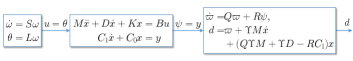
Figure 1: Illustration of the two-sided interconnection of $\bm{\Sigma}$ with the signal generators (41) and (IV).

Following [21, 30], we show that the moments of system $\bm{\Sigma}$ at the interpolation points $\sigma(S)$ and $\sigma(Q)$ are characterized simultaneously by the steady-state response of signal $d(t)$.

Proposition 8.

Consider the two-sided interconnection of $\bm{\Sigma}$ with the signal generators (41) and (IV), where $u=\theta$ and $\psi=y$. Then, on the manifold $\mathcal{M}=\{(x,\omega)\in\mathbb{R}^{n+\nu}\mid x=\Pi\omega\}$, it holds that

$$\dot{d}=Qd+\Upsilon BL\omega$$ (43)

where $\Upsilon$ is the unique solution of equation (20).

Proof.

From (IV), we have

$$\dot{d}=\dot{\varpi}+(Q\Upsilon M+\Upsilon D-RC_{1})\dot{x}+\Upsilon M\ddot{x},$$ (44)

where $\dot{\varpi}=Q\varpi+R(C_{1}\dot{x}+C_{0}x)$. Moreover, on the manifold $\mathcal{M}$, it hold that $\dot{x}=\Pi\dot{\omega}=\Pi S\omega$, and $\ddot{x}=\Pi S\dot{\omega}=\Pi S^{2}\omega$, which are substituted into (44) and lead to

$$\dot{d}=Q\varpi+\left[RC_{0}\Pi+(Q\Upsilon M+\Upsilon D)\Pi S+\Upsilon M\Pi S^{2}\right]\omega.$$ (45)

Observe that (19) and (20) implies that

$$RC_{0}\Pi+\Upsilon D\Pi S+\Upsilon M\Pi S^{2}$$

$$= Q^{2}\Upsilon M\Pi+Q\Upsilon D\Pi+\Upsilon BL-QR_{1}\Pi$$

$$= Q(Q\Upsilon M+\Upsilon D-RC_{1})\Pi+\Upsilon BL.$$

Consequently, (45) is further written as

$$\dot{d} =Q\left[\varpi+(Q\Upsilon M+\Upsilon D-RC_{1})x+\Upsilon M\dot{x}\right]+BL\omega$$

$$=Qd+BL\omega,$$

which completes the proof. ∎

With the above result, we are ready to determine the second-order reduced model that matches the moments of $\bm{\Sigma}$ at both $\sigma(S)$ and $\sigma(Q)$. Note that this model is within the families of second-order reduced models defined in (34) and (35) with particular choice of $G$ and $H$, respectively.

Theorem 2.

Consider a linear second-order system $\bm{\Sigma}$ in (1) and let $S,Q\in\mathbb{C}^{\nu\times\nu}$ be such that $\sigma(S)\cap\sigma(Q)\cap\Omega=\emptyset$. Let $L\in\mathbb{C}^{p\times\nu}$, $R\in\mathbb{C}^{\nu\times q}$ be such that the pair $(L,S)$ is observable and the pair $(Q,R)$ is controllable. Suppose $\Pi\in\mathbb{C}^{n\times\nu}$ and $\Upsilon\in\mathbb{C}^{\nu\times n}$ are the unique solutions of (19) and (20), respectively, and $\Upsilon\Pi$ is nonsingular, and denote

$$\Pi^{\dagger}:=(\Upsilon\Pi)^{-1}\Upsilon,\ \text{and}\ \Upsilon^{\dagger}:=\Pi(\Upsilon\Pi)^{-1}$$ (46)

as the left pseudo inverse of $\Pi$ and the right pseudo inverse of $\Upsilon$, respectively. Let $\hat{\Omega}$ be the set defined in (29), which satisfies $\hat{\Omega}\cap\sigma(S)\cap\sigma(Q)=\emptyset$.

1. The unique model $\bm{\hat{\Sigma}}_{G}$ in (34) that matches the moments of $\bm{\Sigma}$ at $\sigma(S)$ and $\sigma(Q)$ simultaneously is given by

   $$F_{2}=\Pi^{\dagger}M\Pi,F_{1}=\Pi^{\dagger}D\Pi,\Pi,G=\Pi^{\dagger}B,H_{1}=C_{1}\Pi.$$ (47)

2. The unique model $\bm{\hat{\Sigma}}_{H}$ in (35) that matches the moments of $\bm{\Sigma}$ at $\sigma(S)$ and $\sigma(Q)$ simultaneously is given by

   $$F_{2}=\Upsilon M\Upsilon^{\dagger},F_{1}=\Upsilon D\Upsilon^{\dagger},H_{1}=C_{1}\Upsilon^{\dagger},H_{0}=C_{0}\Upsilon^{\dagger}.$$ (48)

3. The reduced models $\bm{\hat{\Sigma}}_{G}$ and $\bm{\hat{\Sigma}}_{H}$ are equivalent.

Proof.

We start with the proof for $\bm{\hat{\Sigma}}_{G}$. With the parameters in (47), we obtain $F_{0}=\Pi^{\dagger}K$, and $H_{0}=C_{0}\Pi$. Consider a system $\bm{\hat{\Sigma}}_{G}$ in form of (34), which connects the signal generator

$$\dot{w}=Qw+R\hat{\psi},w(0)=0,$$

$$\zeta=w+(QPF_{2}+PF_{1}-RH_{1})\xi+PF_{2}\dot{\xi}.$$

as a downstream system with $\hat{\psi}=\eta$. Then, the system $\bm{\hat{\Sigma}}_{G}$ matches the moments $\Upsilon B$, with $\Upsilon$ the unique solution of (20), at $\sigma(Q)$ if and only if

$$\dot{\zeta} =Q\zeta+\Upsilon Bu$$

$$=Qw+(Q^{2}PF_{2}+QPF_{1}-QRH_{1})\xi+QPF_{2}\dot{\xi}+\Upsilon Bu.$$ (49)

We refer [28, 30] for similar reasoning in the case of first-order systems. Note that

$$\dot{\zeta}= \dot{w}+(QPF_{2}+PF_{1}-RH_{1})\dot{\xi}+PF_{2}\ddot{\xi}$$

$$= Qw+R\left[H_{1}\dot{\xi}+(C_{0}\Pi+C_{1}\Pi S-H_{1}S)\xi\right]$$

$$-RH_{1}\dot{\xi}+QPF_{2}\dot{\xi}+PF_{1}\dot{\xi}+PF_{2}\ddot{\xi}$$

$$= Qw+R(C_{0}\Pi+C_{1}\Pi S-H_{1}S)\xi$$

$$+QPF_{2}\dot{\xi}+PGu-P(GL-F_{2}S^{2}-F_{1}S)\xi.$$ (50)

Therefore, from (IV) and (IV), the system $\bm{\hat{\Sigma}}_{G}$ matches the moments $\Upsilon B$, if and only if the parameters $F_{1}$, $F_{2}$, $G$ and $H_{1}$ in $\bm{\hat{\Sigma}}_{G}$ satisfy

$$PG=\Upsilon B,$$

and

$$Q^{2}PF_{2}+QPF_{1}+P(GL-F_{2}S^{2}-F_{1}S)$$

$$=R(C_{0}\Pi+C_{1}\Pi S-H_{1}S)+QRH_{1}.$$ (51)

It is verified that $P=\Upsilon\Pi$ is the unique solution of (IV) due to $\hat{\Omega}\cap\sigma(Q)=\emptyset$. Moreover, since $\Upsilon$ and $\Pi$ are unique, the parameter matrices of $\bm{\hat{\Sigma}}_{G}$ in (47) is unique.

The proof for $\bm{\hat{\Sigma}}_{H}$ with parameters in (48) follows similar arguments. Besides, the equivalence of $\bm{\hat{\Sigma}}_{G}$ and $\bm{\hat{\Sigma}}_{H}$ follows from the nonsingularity of $\Upsilon\Pi$, with which there exists a coordination transformation between the two systems. ∎

IV-A Moment Matching With Pole Placement

In this section, we extend the arguments in [38, 39] to consider the pole placement problem in the reduced-order modeling of second-order systems, and we derive explicit reduced second-order models that simultaneously possess a set of prescribed poles and match desired high-order moments.

Specifically, we consider $\bm{\Sigma}$ in (1) and the family of approximations $\bm{\hat{\Sigma}}_{G}$ as in (34) that matches the moments of $\bm{\Sigma}$ at $\sigma(S)$ with $S\in\mathbb{C}^{\nu\times\nu}$. The objective is to find the parameter matrices $F_{1}$, $F_{2}$, $G$, and $H_{1}$ such that $\bm{\hat{\Sigma}}_{G}$ has the poles at prescribed locations $\lambda_{1},\lambda_{2},...,\lambda_{\kappa}$, where $\kappa\leq\nu$, and $\lambda_{i}\notin\sigma(S)\cap\Omega$ with $\Omega$ defined in (7).

Define $Q_{\mathrm{p}}\in\mathbb{C}^{\kappa\times\kappa}$ such that $\sigma(Q_{\mathrm{p}})=\{\lambda_{1},\lambda_{2},...,\lambda_{\kappa}\}$. Due to $\sigma(Q_{\mathrm{p}})\cap\Omega=\emptyset$, the second-order Sylvester equation

$$Q_{\mathrm{p}}^{2}\Upsilon_{\mathrm{p}}M+Q_{\mathrm{p}}\Upsilon_{\mathrm{p}}D+\Upsilon_{\mathrm{p}}K=R_{\mathrm{p}}C_{\mathrm{p}0}+Q_{\mathrm{p}}R_{\mathrm{p}}C_{\mathrm{p}1}.$$ (52)

has the unique solution $\Upsilon_{\mathrm{p}}\in\mathbb{C}^{\kappa\times n}$, where $R_{\mathrm{p}}\in\mathbb{C}^{\kappa\times q}$ is any matrix such that the pair $(Q_{\mathrm{p}},R_{\mathrm{p}})$ is controllable, and $C_{\mathrm{p}0},C_{\mathrm{p}1}\in\mathbb{C}^{q\times n}$ such that $C_{\mathrm{p}0}\Pi=C_{\mathrm{p}1}\Pi=0$, i.e. $C_{\mathrm{p}0}^{*}\in\ker(\Pi)$ and $C_{\mathrm{p}1}^{*}\in\ker(\Pi)$ with $\Pi$ the unique solution of (19).

Then, we impose linear constraints on the free parameters of the reduced model $\bm{\hat{\Sigma}}_{G}$ such that the reduced model $\bm{\hat{\Sigma}}_{G}$ has poles at $\sigma(Q_{\mathrm{p}})$.

Theorem 3.

Consider $\bm{\hat{\Sigma}}_{G}$ in (34) as a reduced model that matches the moments of the system (1) at $\sigma(S)$. Let $\Pi$ and $\Upsilon_{\mathrm{p}}\in\mathbb{C}^{\kappa\times n}$ be the unique solutions of the second-order Sylvester equations in (19) and (52), respectively. Assume that $\mathrm{rank}(\Upsilon_{\mathrm{p}}\Pi)=\kappa$. If the following constraints hold

$$\Upsilon_{\mathrm{p}}\Pi F_{2} =\Upsilon_{\mathrm{p}}M\Pi,$$ (53a)

$$\Upsilon_{\mathrm{p}}\Pi F_{1} =\Upsilon_{\mathrm{p}}D\Pi,$$ (53b)

$$\Upsilon_{\mathrm{p}}\Pi G =\Upsilon_{\mathrm{p}}B,$$ (53c)

then $\sigma(Q_{\mathrm{p}})=\{\lambda_{1},\lambda_{2},...,\lambda_{\kappa}\}\subseteq\hat{\Omega}$ with $\hat{\Omega}$ in (29) the set of poles of the reduced model $\bm{\hat{\Sigma}}_{G}$.

Proof.

Observe that $\hat{\Omega}$ of the reduced model $\bm{\hat{\Sigma}}_{G}$ is characterized by the solution of the following determinant equation

$$|\rho(\lambda)|=|\lambda^{2}F_{2}+\lambda F_{1}+(GL-F_{2}S^{2}-F_{1}S)|=0.$$

With the equations in (53), the matrix polynomial in the above determinant can be rewritten as

$$\Upsilon_{\mathrm{p}}\Pi\rho(\lambda)= \Upsilon_{\mathrm{p}}\Pi\left[\lambda^{2}F_{2}+\lambda F_{1}+(GL-F_{2}S^{2}-F_{1}S)\right]$$

$$= \lambda^{2}\Upsilon_{\mathrm{p}}M\Pi+\lambda\Upsilon_{\mathrm{p}}D\Pi$$

$$+\Upsilon_{\mathrm{p}}BL-\Upsilon_{\mathrm{p}}M\Pi S^{2}-\Upsilon_{\mathrm{p}}D\Pi S.$$ (54)

Moreover, it follows from the second-order Sylvester equation (19) that

$$\Upsilon_{\mathrm{p}}BL-\Upsilon_{\mathrm{p}}M\Pi S^{2}-\Upsilon_{\mathrm{p}}D\Pi S$$

$$= \Upsilon_{\mathrm{p}}(M\Pi S^{2}+D\Pi S+K\Pi)-\Upsilon_{\mathrm{p}}M\Pi S^{2}-\Upsilon_{\mathrm{p}}D\Pi S$$

$$= \Upsilon_{\mathrm{p}}K\Pi.$$ (55)

Let (52) be post-multiplied by $\Pi$, which yields

$$\Upsilon_{\mathrm{p}}K\Pi=-Q_{\mathrm{p}}^{2}\Upsilon_{\mathrm{p}}M\Pi-Q_{\mathrm{p}}\Upsilon_{\mathrm{p}}D\Pi,$$ (56)

as $C_{\mathrm{p}0}$ and $C_{\mathrm{p}1}$ are chosen such that $C_{\mathrm{p}0}\Pi=C_{\mathrm{p}1}\Pi=0$.

Combining (IV-A), (IV-A), and (56), we obtain

$$\Upsilon_{\mathrm{p}}\Pi\rho(\lambda)=(\lambda I-Q_{\mathrm{p}})\left[(\lambda I+Q_{\mathrm{p}})\Upsilon_{\mathrm{p}}M\Pi+\Upsilon_{\mathrm{p}}D\Pi\right].$$ (57)

Notice that $\lambda\in\sigma(Q_{\mathrm{p}})$ if and only if there exists a left eigenvector $v\in\mathbb{C}^{\kappa}$ such that $v^{*}(\lambda I-Q_{\mathrm{p}})=0$. Then, we obtain from (57) that

$$v^{*}(\lambda I-Q_{\mathrm{p}})\left[(\lambda I+Q_{\mathrm{p}})\Upsilon_{\mathrm{p}}M\Pi+\Upsilon_{\mathrm{p}}D\Pi\right]=0$$

i.e. $v^{*}\Upsilon_{\mathrm{p}}\Pi\rho(\lambda)=\bar{v}^{*}\rho(\lambda)=0$ with $\bar{v}=(\Upsilon_{\mathrm{p}}\Pi)^{*}v\in\mathbb{C}^{\nu}$. It means that there is a vector $\bar{v}_{r}\in\mathbb{C}^{\nu}$ such that $\rho(\lambda)\bar{v}_{r}=0$, i.e. $F_{2}^{-1}(\lambda^{2}F_{2}+\lambda F_{1}+(GL-F_{2}S^{2}-F_{1}S))=0$, which is equivalent to

$$\left(\lambda I-\begin{bmatrix}0&I\\ -F_{2}^{-1}(GL-F_{2}S^{2}-F_{1}S)&-F_{2}^{-1}F_{1}\end{bmatrix}\right)\begin{bmatrix}\bar{v}_{r}\\ \lambda\bar{v}_{r}\end{bmatrix}=0,$$

Therefore, for any $\lambda\in\sigma(Q_{\mathrm{p}})$, we have $|\rho(\lambda)|=0$, i.e. $\lambda\in\hat{\Omega}$.

$\lambda\in\hat{\Omega}$ if and only if there is a nonzero vector $v\in\mathbb{C}^{2\nu}$ such that

which is equivalent to $\bar{v}\in$ such that $\rho(\lambda)\bar{v}=0,$ with $v=\begin{bmatrix}\lambda\bar{v}^{*}&\bar{v}^{*}\end{bmatrix}^{*}$. Therefore, we obtain from (57) that $\Upsilon_{\mathrm{p}}\Pi\rho(\lambda)\bar{v}=0$, i.e.

$$(\lambda I-Q_{\mathrm{p}})\left[(\lambda I+Q_{\mathrm{p}})\Upsilon_{\mathrm{p}}M\Pi+\Upsilon_{\mathrm{p}}D\Pi\right]\bar{v}=0$$

Consequently, any $\lambda_{i}\in\sigma(Q_{\mathrm{p}})$, i.e. $|\lambda_{i}I-Q_{\mathrm{p}}|=0$, also leads to $|\rho(\lambda_{i})|=0$, which means $\lambda_{i}\in\hat{\Omega}$. ∎

IV-B Moment Matching of First-Order Derivatives

Next, we study the reduced second-order systems that matches the moments of both zero and first order derivative of the transfer function

$$W(s)=C(Ms^{2}+Ds+K)^{-1}B,$$ (58)

where $C=C_{0}$ and $C_{1}=0$ in the original system (1).

Denote

$$W_{L}(s): =-C(Ms^{2}+Ds+K)^{-1}$$ (59a)

$$W_{R}(s): =(2Ms+D)(Ms^{2}+Ds+K)^{-1}B$$ (59b)

Then, the first-order derivative of $W(s)$ is $W^{\prime}(s)=W_{L}(s)\cdot W_{R}(s),$ which has a state-space representation as

$$\bm{\Sigma}^{\prime}:\ \begin{cases}M\ddot{x}(t)+D\dot{x}(t)+Kx(t)&=Bu(t),\\ M\ddot{z}(t)+D\dot{z}(t)+Kz(t)&=2M\dot{x}(t)+Dx(t),\\ -Cz(t)&=y(t),\end{cases}$$ (60)

with $z(t)\in\mathbb{R}^{n}$ and $y(t)\in\mathbb{R}$.

Consider the following signal generator

$$\dot{\varpi}=S\varpi+L^{*}\psi,\varpi(0)=0,$$

$$d=\varpi+(S\Upsilon M+\Upsilon D)z+\Upsilon M\dot{z},$$ (61)

where $\Upsilon\in\mathbb{R}^{\nu\times n}$ is the unique solution of the second-order Sylvester equation:

$$S^{2}\Upsilon M+S\Upsilon D+\Upsilon K=-L^{*}C,$$ (62)

since $\sigma(S)\cap\Omega=\emptyset$ is assumed. We then connect the system $\bm{\Sigma}^{\prime}$ with the signal generators (41) and (IV-B), where $u=\theta$ and $\psi=y$, see Fig. 2. The following result is obtained with the property of the signal $d(t)$ in (IV-B).

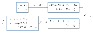
Figure 2: Illustration of the interconnection of $\bm{\Sigma}^{\prime}$ with the signal generators (41) and (IV-B).

Theorem 4.

Consider the system $\bm{\Sigma}^{\prime}$ in (60), which is connected to the signal generators (41) and (IV-B) with $u=\theta$ and $\psi=y$. Let $\Pi$ and $\Upsilon$ be the unique solutions of (19) and (62), respectively, and assume that $\Omega\subset\mathbb{C}^{-}$ and $\sigma(S)\subset\mathbb{C}^{0}$. Then the moments of $\bm{\Sigma}^{\prime}$ at $\sigma(S)$ are in a one-to-one relation with the steady-state response of the signal $d(t)$ in (IV-B).

Proof.

The scheme of proving this result follows similar arguments as in [28, 30], but the details require nontrivial modifications due to the second-order structure of the system. Observe that

$$\dot{d} =\dot{\varpi}+(S\Upsilon M+\Upsilon D)\dot{z}+\Upsilon M\ddot{z}$$

$$=S\varpi-L^{*}Cz+S\Upsilon M\dot{z}+\Upsilon(\tilde{u}-Kz),$$

which, using $\tilde{u}=\tilde{y}=2M\dot{x}+Dx$ and (62), leads to

$$\dot{d}= S\varpi-L^{*}Cz+S\Upsilon M\dot{z}+2\Upsilon M\dot{x}+2\Upsilon Dx$$

$$-(-L^{*}C-S^{2}\Upsilon M-S\Upsilon D)z,$$

$$= S\left[\varpi+(S\Upsilon M+\Upsilon D){z}+\Upsilon M\dot{z}\right]+\Upsilon(2M\dot{x}+Dx)$$

$$= Sd+\Upsilon\begin{bmatrix}D&2M\end{bmatrix}\begin{bmatrix}x(t)\\ \dot{x}(t)\end{bmatrix},$$

Since $M(\ddot{x}-\Pi\ddot{\omega})+D(\dot{x}-\Pi\dot{\omega})+K({x}-\Pi{\omega})=M\ddot{x}+D\dot{x}+K{x}-(M\Pi S^{2}+D\Pi S+K\Pi{\omega})\omega=Bu-BL\omega=0,$ we obtain

$$\begin{bmatrix}x(t)\\ \dot{x}(t)\end{bmatrix}=\begin{bmatrix}\Pi\\ \Pi S\end{bmatrix}\omega+e^{\mathcal{A}t}\begin{bmatrix}x(0)-\Pi\omega(0)\\ \dot{x}(0)-\Pi S\omega(0)\\ \end{bmatrix},$$

which yields

$$\dot{d}= Sd+(2\Upsilon M\Pi S+\Upsilon D\Pi)\omega+\Delta_{d},$$ (63)

with $\Delta_{d}:=\Upsilon\begin{bmatrix}D&2M\end{bmatrix}e^{\mathcal{A}t}\begin{bmatrix}x(0)-\Pi\omega(0)\\ \dot{x}(0)-\Pi S\omega(0)\\ \end{bmatrix}$. Denote $\mathscr{D}(s)$ as the Laplace transform of $d(t)$. Note that the term $\Delta_{d}$ vanishes in the steady-state response, and thus

$$\mathscr{D}(s)=(sI-S)^{-1}\Upsilon(2M\Pi S+D\Pi)\mathscr{W}(s),$$

where $\mathscr{W}(s)$ denotes the Laplace transform of $\omega(t)$. Moreover, we obtain from (41) that $\mathscr{W}(s):=(sI-S)^{-1}\omega(0)$, which leads to

$$\mathscr{D}(s)=(sI-S)^{-1}\Upsilon(2Ms+D)\Pi(sI-S)^{-1}\omega(0)$$

$$-2(sI-S)^{-1}\Upsilon M\Pi\omega(0).$$ (64)

Denote $\mathscr{F}(s)=(Ms^{2}+Ds+K)^{-1}$. Then, the following two equations hold.

$$(sI-S)^{-1}\Upsilon\mathscr{F}^{-1}$$

$$= (sI-S)^{-1}(\Upsilon Ms^{2}+\Upsilon Ds+\Upsilon K)$$

$$= (sI-S)^{-1}(\Upsilon Ms^{2}+\Upsilon Ds-L^{*}C-S^{2}\Upsilon M-S\Upsilon D)$$

$$= (sI+S)\Upsilon M+\Upsilon D-L^{*}C,$$

and

$$\mathscr{F}^{-1}\Pi(sI-S)^{-1}$$

$$= (M\Pi s^{2}+D\Pi s+K\Pi)(sI-S)^{-1}$$

$$= (M\Pi s^{2}+D\Pi s+BL-M\Pi S^{2}-D\Pi S)(sI-S)^{-1}$$

$$= M\Pi(sI+S)+D\Pi+BL.$$

Therefore, and we can rewrite the first term of $\mathscr{D}(s)$ as

$$\mathscr{D}_{1}(s) =(sI-S)^{-1}\Upsilon\mathscr{F}^{-1}(s)\mathscr{F}(s)(2Ms+D)$$

$$\quad\quad\quad\quad\cdot\mathscr{F}(s)\mathscr{F}^{-1}(s)\Pi(sI-S)^{-1}\omega(0),$$

$$=\left[(sI+S)\Upsilon M+\Upsilon D-L^{*}C\right]\mathscr{F}(s)(2Ms+D)$$

$$\quad\quad\quad\quad\cdot\mathscr{F}(s)\left[M\Pi(sI+S)+D\Pi+BL\right]\omega(0)$$

$$=-L^{*}C\mathscr{F}(s)(2Ms+D)\mathscr{F}(s)BL+\cdots$$

As a result, the steady-state response of $d(t)$ contains terms of the form $L^{*}\frac{W(s_{i})}{(s-s_{i})^{2}}L,$ with $s_{i}\in\sigma(S)$, which proves the claim. ∎

Next, we present a second-order reduced model which matches the moments of $W(s)$ and $W^{\prime}(s)$ simultaneously at the interpolation points $\sigma(S)$. Thereby, we suppose $H_{1}=0$ and $H_{0}=H$ in (34) and (35).

Theorem 5.

Consider a linear second-order system $\bm{\Sigma}$ in (1) and let $S\in\mathbb{C}^{\nu\times\nu}$, $L\in\mathbb{C}^{p\times\nu}$ be such that the pair $(L,S)$ is observable, and $\Pi\in\mathbb{C}^{n\times\nu}$ and $\Upsilon\in\mathbb{C}^{\nu\times n}$ are the unique solutions of (19) and (62), respectively, such that $\Upsilon\Pi$ is nonsingular. Then the following statements hold.

1. A model $\bm{\hat{\Sigma}}_{G}$ that matches the moments of $W(s)$ and $W^{\prime}(s)$ at $\sigma(S)$ is given by

   $$F_{2}=\Pi^{\dagger}M\Pi,F_{1}=\Pi^{\dagger}D\Pi,G=\Pi^{\dagger}B,$$ (65)

   with $\Pi^{\dagger}:=(\Upsilon\Pi)^{-1}\Upsilon.$

2. A $\bm{\hat{\Sigma}}_{H}$ that matches the moments of $W(s)$ and $W^{\prime}(s)$ at $\sigma(S)$ is given by

   $$F_{2}=\Upsilon M\Upsilon^{\dagger},F_{1}=\Upsilon D\Upsilon^{\dagger},H=C\Upsilon^{\dagger},$$

   with $\Upsilon^{\dagger}:=\Pi(\Upsilon\Pi)^{-1}$.

3. The reduced models $\bm{\hat{\Sigma}}_{G}$ and $\bm{\hat{\Sigma}}_{H}$ are equivalent.

Proof.

First, with the reduced matrices in (65), we obtain $F_{0}=\Pi^{\dagger}K$ and $H=C\Pi$. It is not hard to verify according to Proposition 3 that $\bm{\hat{\Sigma}}_{G}$ matches the moments of $W(s)$ at $\sigma(S)$. Then, we prove that $\bm{\hat{\Sigma}}_{G}$ also matches the moments of $W^{\prime}(s)$, which means that $W_{L}(s_{i})W_{R}(s_{i})=-H(F_{2}s_{i}^{2}+F_{1}s_{i}+F_{0})^{-1}(2F_{2}s_{i}+F_{1})(F_{2}s_{i}^{2}+F_{1}s_{i}+F_{0})^{-1}B$, for all $s_{i}\in\sigma(S)$, with the transfer function $W_{L}(s)$, $W_{R}(s)$ defined in (59).

Observe that $2F_{2}s_{i}+F_{1}=P\Upsilon(2Ms_{i}+D)\Pi$, where $P:=(\Upsilon\Pi)^{-1}$. Therefore, the moment matching is achieved if

$$C(Ms_{i}^{2}+Ds_{i}+K)^{-1}=C\Pi(F_{2}s_{i}^{2}+F_{1}s_{i}+F_{0})^{-1}P\Upsilon,$$ (66)

and

$$(Ms_{i}^{2}+Ds_{i}+K)^{-1}B=\Pi(F_{2}s_{i}^{2}+F_{1}s_{i}+F_{0})^{-1}P\Upsilon B.$$ (67)

It follows from the second-order Sylvester equations (19) and (20) that

$$S^{2}P^{-1}F_{2}+SP^{-1}F_{1}+P^{-1}F_{0}=L^{*}C\Pi,$$

$$F_{2}S^{2}+F_{1}S+F_{0}=P\Upsilon BL,$$

with $F_{2}$, $F_{1}$, and $F_{0}$ in (65). Thus, (66) and (67) are satisfied.

Besides, we note that the systems $\bm{\hat{\Sigma}}_{G}$ and $\bm{\hat{\Sigma}}_{H}$ are equivalent, as there exists a coordination transformation between the two systems due to the nonsingularity of $\Upsilon\Pi$. ∎

V Second-Order Loewner Framework

An overview of the Loewner framework is found in [40, 41, 42], which provides results connecting this rational interpolation tool with system theory. In the paper, we extend the Loewner framework in the first order setting to the second-order one. Specifically, we consider $C_{1}=0$ and $C_{0}=C$. The preliminary results of this part can be found in [43].

In the tangential interpolation problem, we collect the samples of input/output frequency response data of a system directionally on the left and on the right. Specifically, the right and left tangential interpolation data are defined, respectively, as

$$\{\alpha_{i},r_{i},w_{i}\mid\alpha_{i}\in\mathbb{C},r_{i}\in\mathbb{C}^{p},w_{i}\in\mathbb{C}^{q}\}_{i=1,2,...,\nu}$$ (68a)

$$\{\beta_{j},l_{j},v_{j}\mid\beta_{j}\in\mathbb{C},l_{j}\in\mathbb{C}^{q},v_{j}\in\mathbb{C}^{p}\}_{j=1,2,...,\nu},$$ (68b)

where $\alpha_{i}$ and $\beta_{j}$ are the right and left driving frequencies, $r_{i}$ and $l_{j}$ are the right and left tangential directions, and $w_{i}$ and $v_{j}$ are the right and left responses. All the data in (68a) can be rearranged compactly as $(\Lambda_{\alpha},\mathcal{R},\mathcal{W})$ and $(\Lambda_{\beta},\mathcal{L},\mathcal{V})$ with

$$\Lambda_{\beta}=\begin{bmatrix}\alpha_{1}&&\\ &\ddots&\\ &&\alpha_{\nu}\end{bmatrix},\ \begin{split}\mathcal{R}&=\begin{bmatrix}r_{1}&\cdots&r_{\nu}\end{bmatrix},\\ \mathcal{W}&=\begin{bmatrix}w_{1}&\cdots&w_{\nu}\end{bmatrix}.\end{split}$$

$$\Lambda_{\alpha}=\begin{bmatrix}\beta_{1}&&\\ &\ddots&\\ &&\beta_{\nu}\end{bmatrix},\ \mathcal{L}=\begin{bmatrix}l_{1}^{\top}\\ \vdots\\ l_{\nu}^{\top}\end{bmatrix},\ \mathcal{V}=\begin{bmatrix}v_{1}^{\top}\\ \vdots\\ v_{\nu}^{\top}\end{bmatrix},$$

The problem is to find a realization in the second-order form as in (1) such that the associated transfer function

$$W(s)=C(Ms^{2}+Ds+K)^{-1}B\in\mathbb{C}^{q\times p}$$

satisfies the right and the left tangential constraints:

$$W(\alpha_{i})r_{i} =w_{i},\forall~{}i.$$

$$l_{j}^{\top}W(\beta_{j}) =v_{j}^{\top},\forall~{}j.$$

Similar to the Loewner framework for first-order systems [40, 41], we establish the Loewner matrix $\mathbb{L}$ and the shifted Loewner matrix $\mathbb{L}_{s}$ for second-order systems as

$$\mathbb{L} =\begin{bmatrix}\frac{v_{1}^{\top}r_{1}-l_{1}^{\top}w_{1}}{\beta_{1}-\alpha_{1}}&\cdots&\frac{v_{1}^{\top}r_{\nu}-l_{1}^{\top}w_{\nu}}{\beta_{1}-\alpha_{\nu}}\\ \vdots&\ddots&\vdots\\ \frac{v_{\nu}^{\top}r_{1}-l_{\nu}^{\top}w_{1}}{\beta_{\nu}-\alpha_{1}}&\cdots&\frac{v_{\nu}^{\top}r_{\nu}-l_{\nu}^{\top}w_{\nu}}{\beta_{\nu}-\alpha_{\nu}}\end{bmatrix},$$ (70)

$$\mathbb{L}_{s} =\begin{bmatrix}\frac{\beta_{1}v_{1}^{\top}r_{1}-\alpha_{1}l_{1}^{\top}w_{1}}{\beta_{1}-\alpha_{1}}&\cdots&\frac{\beta_{1}v_{1}^{\top}r_{\nu}-\alpha_{\nu}l_{1}^{\top}w_{\nu}}{\beta_{1}-\alpha_{\nu}}\\ \vdots&\ddots&\vdots\\ \frac{\beta_{\nu}v_{\nu}^{\top}r_{1}-\alpha_{1}l_{\nu}^{\top}w_{1}}{\beta_{\nu}-\alpha_{1}}&\cdots&\frac{\beta_{\nu}v_{\nu}^{\top}r_{\nu}-\alpha_{\nu}l_{\nu}^{\top}w_{\nu}}{\beta_{\nu}-\alpha_{\nu}}\end{bmatrix}.$$ (71)

Furthermore, we also introduce the double-shifted Loewner matrix $\mathbb{L}_{ss}$ as

$$\mathbb{L}_{ss}=\begin{bmatrix}\frac{\beta_{1}^{2}v_{1}^{\top}r_{1}-\alpha_{1}^{2}l_{1}^{\top}w_{1}}{\beta_{1}-\alpha_{1}}&\cdots&\frac{\beta_{1}^{2}v_{1}^{\top}r_{\nu}-\alpha_{\nu}^{2}l_{1}^{\top}w_{\nu}}{\beta_{1}-\alpha_{\nu}}\\ \vdots&\ddots&\vdots\\ \frac{\beta_{\nu}^{2}v_{\nu}^{\top}r_{1}-\alpha_{1}^{2}l_{\nu}^{\top}w_{1}}{\beta_{\nu}-\alpha_{1}}&\cdots&\frac{\beta_{\nu}^{2}v_{\nu}^{\top}r_{\nu}-\alpha_{\nu}^{2}l_{\nu}^{\top}w_{\nu}}{\beta_{\nu}-\alpha_{\nu}}\end{bmatrix}.$$ (72)

Denote the tangential versions of the generalized controllability and observability matrices as

$$\mathcal{X} =[(M\alpha_{1}^{2}+D\alpha_{1}+K)^{-1}Br_{1}$$

$$\quad\quad\cdots(M\alpha_{\nu}^{2}+D\alpha_{\nu}+K)^{-1}Br_{\nu}]$$

$$\mathcal{Y} =\begin{bmatrix}l_{1}^{\top}C(M\beta_{1}^{2}+D\beta_{1}+K)^{-1}\\ \vdots\\ l_{\nu}^{\top}C(M\beta_{\nu}^{2}+D\beta_{\nu}+K)^{-1}\end{bmatrix}.$$ (73)

The following result then shows how the matrices $\mathbb{L}$, $\mathbb{L}_{s}$, and $\mathbb{L}_{ss}$ are related with $\mathcal{X}$ and $\mathcal{Y}$.

Lemma 3.

Consider the generalized controllability and observability matrices $\mathcal{X}$ and $\mathcal{Y}$ in (73). Then, the Loewner matrix $\mathcal{L}$ in (70), the shifted Loewner matrix $\mathcal{L}_{s}$ in (71), and the double-shifted Loewner matrix $\mathcal{L}_{ss}$ in (72) can be represented as

$$\mathbb{L} =-\Lambda_{\beta}\mathcal{Y}M\mathcal{X}-\mathcal{Y}M\mathcal{X}\Lambda_{\alpha}-\mathcal{Y}D\mathcal{X},$$ (74a)

$$\mathbb{L}_{s} =-\Lambda_{\beta}\mathcal{Y}M\mathcal{X}\Lambda_{\alpha}+\mathcal{Y}K\mathcal{X},$$ (74b)

$$\mathbb{L}_{ss} =\Lambda_{\beta}\mathcal{Y}D\mathcal{X}\Lambda_{\alpha}+\Lambda_{\beta}\mathcal{Y}K\mathcal{X}+\mathcal{Y}K\mathcal{X}\Lambda_{\alpha}.$$ (74c)

Proof.

Note that

$$v_{j}^{\top}r_{i}-l_{j}^{\top}w_{i}$$

$$= l_{j}^{\top}C\left[(M\beta_{j}^{2}+D\beta_{j}+K)^{-1}-(M\alpha_{i}^{2}+D\alpha_{i}+K)^{-1}\right]Br_{i}$$

$$= l_{j}^{\top}C(M\beta_{j}^{2}+D\beta_{j}+K)^{-1}\left[M(\alpha_{i}^{2}-\beta_{j}^{2})+D(\alpha_{i}-\beta_{j})\right]$$

$$(M\alpha_{i}^{2}+D\alpha_{i}+K)^{-1}Br_{i}$$

$$= (\alpha_{i}-\beta_{j})l_{j}^{\top}C(M\beta_{j}^{2}+D\beta_{j}+K)^{-1}\left[M(\alpha_{i}+\beta_{j})+D\right]$$

$$(M\alpha_{i}^{2}+D\alpha_{i}+K)^{-1}Br_{i}$$

$$= (\alpha_{i}-\beta_{j})\mathcal{Y}_{j}\left[M(\alpha_{i}+\beta_{j})+D\right]\mathcal{X}_{i}$$

Thus, the $(i,j)$-element of $\mathbb{L}$ is given by

$$[\mathbb{L}]_{ij}=-\mathcal{Y}_{j}\left[M(\alpha_{i}+\beta_{j})+D\right]\mathcal{X}_{i},$$

which leads to (74a).

Analogously, we can find

$$\beta_{j}v_{j}^{\top}r_{i}-\alpha_{i}l_{j}^{\top}w_{i}=(\alpha_{i}-\beta_{j})\mathcal{Y}_{j}\left[M\alpha_{i}\beta_{j}-K\right]\mathcal{X}_{i}$$

$$\beta_{j}^{2}v_{j}^{\top}r_{i}-\alpha_{i}^{2}l_{j}^{\top}w_{i}=-(\alpha_{i}-\beta_{j})\mathcal{Y}_{j}\left[D\alpha_{i}\beta_{j}+K(\alpha_{i}+\beta_{j})\right]\mathcal{X}_{i}.$$

yielding that

$$[\mathbb{L}_{s}]_{ij} =-\mathcal{Y}_{j}\left[M\alpha_{i}\beta_{j}-K\right]\mathcal{X}_{i},$$ (75)

$$[\mathbb{L}_{ss}]_{ij} =\mathcal{Y}_{j}\left[D\alpha_{i}\beta_{j}-K(\alpha_{i}+\beta_{j})\right]\mathcal{X}_{i}.$$ (76)

Therefore, the equations (74b) and (74c) follow. ∎

In the sequel, the matrices $\mathbb{L}$, $\mathbb{L}_{s}$, and $\mathbb{L}_{ss}$ are characterized as the solutions of Sylvester equations.

Lemma 4.

The Loewner matrix $\mathbb{L}$ in (70) is the unique solution of the Sylvester equation,

$$\Lambda_{\beta}\mathbb{L}-\mathbb{L}\Lambda_{\alpha}=\mathcal{V}\mathcal{R}-\mathcal{L}\mathcal{W},$$ (77)

the shifted Loewner matrix is the unique solution of the Sylvester equation

$$\Lambda_{\beta}\mathbb{L}_{s}-\mathbb{L}_{s}\Lambda_{\alpha}=\Lambda_{\beta}\mathcal{V}\mathcal{R}-\mathcal{L}\mathcal{W}\Lambda_{\alpha},$$ (78)

and furthermore, the double-shifted Loewner matrix $\mathcal{L}_{ss}$ in (72) is the unique solution of the Sylvester equation

$$\Lambda_{\beta}\mathbb{L}_{ss}-\mathbb{L}_{ss}\Lambda_{\alpha}=\Lambda_{\beta}^{2}\mathcal{V}\mathcal{R}-\mathcal{L}\mathcal{W}\Lambda_{\alpha}^{2}.$$ (79)

Proof.

Upon multiplication of (74a) with $\Lambda_{\alpha}$ on the right we have

$$\mathcal{Y}M\mathcal{X}\Lambda_{\alpha}^{2}+\mathcal{Y}D\mathcal{X}\Lambda_{\alpha}=-\mathbb{L}\Lambda_{\alpha}-\Lambda_{\beta}\mathcal{Y}M\mathcal{X}\Lambda_{\alpha},$$ (80)

and further obtain from (81) that

$$\mathcal{Y}K\mathcal{X}=\mathbb{L}_{s}+\Lambda_{\beta}\mathcal{Y}M\mathcal{X}\Lambda_{\alpha}.$$ (81)

Letting the equation (19) be multiplied by $\mathcal{Y}$ on the left leads to

$$\mathcal{Y}M\mathcal{X}\Lambda_{\alpha}^{2}+\mathcal{Y}D\mathcal{X}\Lambda_{\alpha}+\mathcal{Y}K\mathcal{X}=\mathcal{Y}B\mathcal{R},$$

$$\Leftrightarrow -\mathbb{L}\Lambda_{\alpha}-\Lambda_{\beta}\mathcal{Y}M\mathcal{X}\Lambda_{\alpha}+\mathbb{L}_{s}+\Lambda_{\beta}\mathcal{Y}M\mathcal{X}\Lambda_{\alpha}=\mathcal{V}\mathcal{R}$$

$$\Leftrightarrow -\mathbb{L}\Lambda_{\alpha}+\mathbb{L}_{s}=\mathcal{V}\mathcal{R},$$ (82)

where the equations (80) and (81) are used. Similarly, multiplying by $\mathcal{X}$ on the right of the equation (20) then yields

$$-\Lambda_{\beta}\mathbb{L}+\mathbb{L}_{s}=\mathcal{L}\mathcal{W},$$ (83)

The Sylvester equations in (77) and (78) are then followed by adding/subtracting appropriate multiples of (V) and (83).

We then proceed to prove the Sylvester equation for the double-shifted Loewner matrix $\mathcal{L}_{ss}$. First, it is not hard to show the following relation from (74):

$$\mathbb{L}_{ss}=-\Lambda_{\beta}\mathbb{L}\Lambda_{\alpha}+\Lambda_{\beta}\mathbb{L}_{s}+\mathbb{L}_{s}\Lambda_{\alpha}.$$ (84)

Then, we have

$$\Lambda_{\beta}\mathbb{L}_{ss}-\mathbb{L}_{ss}\Lambda_{\alpha}$$

$$= -\Lambda_{\beta}^{2}\mathbb{L}\Lambda_{\alpha}+\Lambda_{\beta}^{2}\mathbb{L}_{s}+\Lambda_{\beta}\mathbb{L}_{s}\Lambda_{\alpha}$$

$$-(-\Lambda_{\beta}\mathbb{L}\Lambda_{\alpha}^{2}+\Lambda_{\beta}\mathbb{L}_{s}\Lambda_{\alpha}+\mathbb{L}_{s}\Lambda_{\alpha}^{2})$$

$$= \Lambda_{\beta}^{2}(\mathbb{L}\Lambda_{\alpha}+\mathbb{L}_{s})-(-\Lambda_{\beta}\mathbb{L}+\mathbb{L}_{s})\Lambda_{\alpha}^{2}$$

$$= \Lambda_{\beta}^{2}\mathcal{V}\mathcal{R}-\mathcal{L}\mathcal{W}\Lambda_{\alpha}^{2}.$$

Therefore, (79) is proven. ∎

In the following, we will show how to use different pairwise combinations of matrices $\mathbb{L}$, $\mathbb{L}_{s}$, and $\mathbb{L}_{ss}$ to construct parameterized families of interpolants possessing the second-order structure.

Theorem 6.

Let $\mathbb{L}\in\mathbb{C}^{\nu\times\nu}$ and $\mathbb{L}_{s}\in\mathbb{C}^{\nu\times\nu}$ be the Loewner matrix and shifted Loewner matrix, respectively, associated to the right and left tangential data $(\Lambda_{\alpha},\mathcal{R},\mathcal{W})$ and $(\Lambda_{\beta},\mathcal{L},\mathcal{V})$. Define a reduced-order model with second-order structure as

$$\hat{M}\ddot{\xi}+(-\mathbb{L}-\Lambda_{\beta}\hat{M}-\hat{M}\Lambda_{\alpha})\dot{\xi}+(\mathbb{L}_{s}+\Lambda_{\beta}\hat{M}\Lambda_{\alpha})\xi =\mathcal{V}u,$$

$$\eta =\mathcal{W}\xi,$$ (85)

where $\hat{M}$ is any square matrix such that the matrix pencil

$$\hat{M}\lambda^{2}+(-\mathbb{L}-\Lambda_{\beta}\hat{M}-\hat{M}\Lambda_{\alpha})\lambda+(\mathbb{L}_{s}+\Lambda_{\beta}\hat{M}\Lambda_{\alpha})$$ (86)

is regular and has no eigenvalues belonging to $\sigma(\Lambda_{\alpha})\cup\sigma(\Lambda_{\beta})$. Then, the model (85) interpolates the tangential data $(\Lambda_{\alpha},\mathcal{R},\mathcal{W})$ and $(\Lambda_{\beta},\mathcal{L},\mathcal{V})$, simultaneously.

Proof.

It is obtained from the tangential constraints on data that $C\mathcal{R}=\mathcal{W}$ and $B\mathcal{L}=\mathcal{V}$. Then, according to Proposition 3, the model (85) interpolates the data $(\Lambda_{\alpha},\mathcal{R},\mathcal{W})$ and $(\Lambda_{\beta},\mathcal{L},\mathcal{V})$ if the following Sylvester equations hold.

$$\hat{M}\Lambda_{\alpha}^{2}+(-\mathbb{L}-\Lambda_{\beta}\hat{M}-\hat{M}\Lambda_{\alpha})\Lambda_{\alpha}+(\mathbb{L}_{s}+\Lambda_{\beta}\hat{M}\Lambda_{\alpha}) =\mathcal{V}\mathcal{R},$$

$$\Lambda_{\beta}^{2}\hat{M}+\Lambda_{\beta}(-\mathbb{L}-\Lambda_{\beta}\hat{M}-\hat{M}\Lambda_{\alpha})+(\mathbb{L}_{s}+\Lambda_{\beta}\hat{M}\Lambda_{\alpha}) =\mathcal{L}\mathcal{W}.$$

These equations are simplified as

$$-\mathbb{L}\Lambda_{\alpha}+\mathbb{L}_{s}=\mathcal{V}\mathcal{R},\ \text{and}\ -\Lambda_{\beta}\mathbb{L}+\mathbb{L}_{s}=\mathcal{L}\mathcal{W},$$ (88)

respectively, which are proved in (V) and (83). Therefore, the model (85) with a free parameter $\hat{M}$ interpolates both the left and right tangential data. ∎

Theorem 6 presents a parameterized family of interpolants (85) possessing the second-order structure with $\hat{M}$ a free parameter. Any $\hat{M}$ that fulfills the matrix pencil condition on (86) will lead to an interpolant of the left and right tangential data. Particularly, we may also choose $\hat{M}=0$, then a first-order model is generated as

$$-\mathbb{L}\dot{\xi}+\mathbb{L}_{s}\xi=\mathcal{V}u,\ \eta=\mathcal{W}\xi,$$

which is consistent with the results for the first-order Loewner framework in [40, 41].

Remark 2.

A parameterized family of interpolants based on the matrices $\mathbb{L}$ and $\mathbb{L}_{s}$ is also presented in [43] with $J$ a free parameter. If $J=-\hat{M}\Lambda_{\alpha}$, the family of interpolants in [43] can be obtained by a coordinate transformation of (85).

Next, we show how to use the pairs $(\mathbb{L},\mathbb{L}_{ss})$ and $(\mathbb{L},\mathbb{L}_{ss})$ to construct an alternative parameterized family of interpolants that possess the second-order structure. Before proceeding, the following lemma is provided to reveal the relation between $\mathbb{L}$, $\mathbb{L}_{s}$, and $\mathbb{L}_{ss}$.

Lemma 5.

The double-shifted Loewner matrix $\mathbb{L}_{ss}$ in (72) and the Loewner matrix $\mathbb{L}$ in (70) are related as

$$-\mathbb{L}\Lambda_{\alpha}^{2}+\mathbb{L}_{ss} =\Lambda_{\beta}\mathcal{V}\mathcal{R}+\mathcal{V}\mathcal{R}\Lambda_{\alpha},$$ (89a)

$$-\Lambda_{\beta}^{2}\mathbb{L}+\mathbb{L}_{ss} =\Lambda_{\beta}\mathcal{L}\mathcal{W}+\mathcal{L}\mathcal{W}\Lambda_{\alpha}.$$ (89b)

Furthermore, $\mathbb{L}_{ss}$ and the shifted Loewner matrix $\mathbb{L}_{s}$ in (71) satisfy

$$-\mathbb{L}_{s}\Lambda_{\alpha}+\mathbb{L}_{ss} =\Lambda_{\beta}\mathcal{V}\mathcal{R},$$ (90a)

$$-\Lambda_{\beta}\mathbb{L}_{s}+\mathbb{L}_{ss} =\mathcal{L}\mathcal{W}\Lambda_{\alpha}.$$ (90b)

Proof.

Using equations (V), (83), and (84), the four equations are obtained as follows.

$$-\mathbb{L}\Lambda_{\alpha}^{2}+\mathbb{L}_{ss} =-\mathbb{L}\Lambda_{\alpha}^{2}-\Lambda_{\beta}\mathbb{L}\Lambda_{\alpha}+\Lambda_{\beta}\mathbb{L}_{s}+\mathbb{L}_{s}\Lambda_{\alpha}$$

$$=(-\mathbb{L}\Lambda_{\alpha}+\mathbb{L}_{s})\Lambda_{\alpha}+\Lambda_{\beta}(-\mathbb{L}\Lambda_{\alpha}+\mathbb{L}_{s})$$

$$=\Lambda_{\beta}\mathcal{V}\mathcal{R}+\mathcal{V}\mathcal{R}\Lambda_{\alpha},$$

$$-\Lambda_{\beta}^{2}\mathbb{L}+\mathbb{L}_{ss} =-\Lambda_{\beta}^{2}\mathbb{L}-\Lambda_{\beta}\mathbb{L}\Lambda_{\alpha}+\Lambda_{\beta}\mathbb{L}_{s}+\mathbb{L}_{s}\Lambda_{\alpha}$$

$$=(-\Lambda_{\beta}\mathbb{L}+\mathbb{L}_{s})\Lambda_{\alpha}+\Lambda_{\beta}(-\Lambda_{\beta}\mathbb{L}+\mathbb{L}_{s})$$

$$=\Lambda_{\beta}\mathcal{L}\mathcal{W}+\mathcal{L}\mathcal{W}\Lambda_{\alpha},$$

$$-\mathbb{L}_{s}\Lambda_{\alpha}+\mathbb{L}_{ss} =-\mathbb{L}_{s}\Lambda_{\alpha}-\Lambda_{\beta}\mathbb{L}\Lambda_{\alpha}+\Lambda_{\beta}\mathbb{L}_{s}+\mathbb{L}_{s}\Lambda_{\alpha}$$

$$=\Lambda_{\beta}(-\mathbb{L}\Lambda_{\alpha}+\mathbb{L}_{s})=\Lambda_{\beta}\mathcal{V}\mathcal{R},$$

$$-\Lambda_{\beta}\mathbb{L}_{s}+\mathbb{L}_{ss} =-\Lambda_{\beta}\mathbb{L}_{s}-\Lambda_{\beta}\mathbb{L}\Lambda_{\alpha}+\Lambda_{\beta}\mathbb{L}_{s}+\mathbb{L}_{s}\Lambda_{\alpha}$$

$$=(-\Lambda_{\beta}\mathbb{L}+\mathbb{L}_{s})\Lambda_{\alpha}=\mathcal{L}\mathcal{W}\Lambda_{\alpha}.$$

That completes the proof. ∎

Using the double-shifted Loewner matrix and the shifted Loewner matrix, we can construct a parameterized family of interpolants with the second-order structure with a free parameter $\hat{K}$.

Theorem 7.

Let $\mathbb{L}_{s}\in\mathbb{C}^{\nu\times\nu}$ and $\mathbb{L}_{ss}\in\mathbb{C}^{\nu\times\nu}$ be the shifted Loewner matrix and double-shifted Loewner matrix, respectively, associated to the right and left tangential data $(\Lambda_{\alpha},\mathcal{R},\mathcal{W})$ and $(\Lambda_{\beta},\mathcal{L},\mathcal{V})$. Suppose $\Lambda_{\alpha}$ and $\Lambda_{\beta}$ are non-singular. Define a reduced-order model with the second-order structure as

$$(-\mathbb{L}_{s}+\hat{K})\ddot{\xi}+(\mathbb{L}_{ss}-\Lambda_{\beta}\hat{K}-\hat{K}\Lambda_{\alpha})\dot{\xi}+\Lambda_{\beta}\hat{K}\Lambda_{\alpha}\xi =\Lambda_{\beta}\mathcal{V}u,$$

$$\eta =\mathcal{W}\Lambda_{\alpha}\xi,$$ (91)

where $\hat{K}$ is any square matrix such that the matrix pencil

$$(-\mathbb{L}_{s}+\hat{K})\lambda^{2}+(-\mathbb{L}_{ss}+\Lambda_{\beta}\hat{K}+\hat{K}\Lambda_{\alpha})\lambda+\Lambda_{\beta}\hat{K}\Lambda_{\alpha}$$

is regular and has no eigenvalues belonging to $\sigma(\Lambda_{\alpha})\cup\sigma(\Lambda_{\beta})$. Then, the model (91) interpolates the tangential data $(\Lambda_{\alpha},\mathcal{R},\mathcal{W})$ and $(\Lambda_{\beta},\mathcal{L},\mathcal{V})$, simultaneously.

Proof.

If $\Lambda_{\alpha}$ and $\Lambda_{\beta}$ are non-singular, the transfer function of the system (91) is represented as

$$\hat{G}(s)=\mathcal{W}\left(\mathbb{M}s^{2}+\mathbb{D}s+\hat{K}\right)^{-1}\mathcal{V},$$

with $\mathbb{M}:=-\Lambda_{\beta}^{-1}\mathbb{L}_{s}\Lambda_{\alpha}^{-1}+\Lambda_{\beta}^{-1}\hat{K}\Lambda_{\alpha}^{-1}$, $\mathbb{D}:=\Lambda_{\beta}^{-1}\mathbb{L}_{ss}\Lambda_{\alpha}^{-1}-\Lambda_{\beta}^{-1}\hat{K}-\hat{K}\Lambda_{\alpha}^{-1}$. Then, we follow a similar reasoning as the proof of Theorem 6. With $C\mathcal{R}=\mathcal{W}$ and $B\mathcal{L}=\mathcal{V}$, $\hat{G}(s)$ interpolates the data $(\Lambda_{\alpha},\mathcal{R},\mathcal{W})$ and $(\Lambda_{\beta},\mathcal{L},\mathcal{V})$ if the following Sylvester equations are satisfied.

$$\Lambda_{\alpha}^{2}\mathbb{M}+\Lambda_{\alpha}\mathbb{D}+\hat{K}=\mathcal{V}\mathcal{R},\ \mathbb{M}\Lambda_{\beta}^{2}+\mathbb{D}\Lambda_{\beta}+\hat{K}=\mathcal{L}\mathcal{W},$$

which are simplified by substituting the expressions of $\mathbb{M}$ and $\mathbb{D}$ as

$$-\Lambda_{\beta}^{-1}\mathbb{L}_{s}\Lambda_{\alpha}+\Lambda_{\beta}^{-1}\mathbb{L}_{ss}=\mathcal{V}\mathcal{R},\ -\Lambda_{\beta}\mathbb{L}_{s}\Lambda_{\alpha}^{-1}+\mathbb{L}_{ss}\Lambda_{\alpha}^{-1}=\mathcal{L}\mathcal{W}.$$

The above equations hold due to Lemma 5. ∎

Theorem 7 also provides a parameterized family of the second-order interpolants with $\hat{K}$ a free parameter. As a special case, we choose choose $\hat{K}=0$, then the model (91) is simplified as

$$-\mathbb{L}_{s}\ddot{\xi}-\mathbb{L}_{ss}\xi=\Lambda_{\alpha}\mathcal{V}u,\ \eta=\mathcal{W}\Lambda_{\beta}\xi.$$

Remark 3.

It is worth emphasizing the presented second-order Loewner frameworks in Theorem 6 and Theorem 7 can be applied to preserve the second-order structure with the Raylegh-Damped hypothesis, i.e., the damping matrix in (1) is constrained as

$$D=\alpha M+\beta K,$$

where $\alpha,\beta\geq 0$, see [44]. To retain the above property in the interplotant (85), we impose $-\mathbb{L}-\Lambda_{\beta}\hat{M}-\hat{M}\Lambda_{\alpha}=\alpha\hat{M}\ddot{\xi}+\beta(\mathbb{L}_{s}+\hat{M}\Lambda_{\alpha}),$ i.e.

$$(\Lambda_{\beta}+\alpha I)\hat{M}+\hat{M}(\beta\Lambda_{\alpha}+I)=-\mathbb{L}+\beta\mathbb{L}_{s}.$$

This means that, the value of $\hat{M}$ is determined by the above Sylvester equation rather than free parameter to choose. Analogously, we can also preserve the Raylegh-Damped hypothesis in interplotant (91) by requiring $\mathbb{L}_{ss}-\Lambda_{\beta}\hat{K}-\hat{K}\Lambda_{\alpha}=\alpha(-\mathbb{L}_{s}+\hat{K})+\beta\Lambda_{\beta}\hat{K}\Lambda_{\alpha}$, which leads to the Sylvester equation to determining $\hat{K}$:

$$\Lambda_{\beta}\hat{K}+\hat{K}(\Lambda_{\beta}+\alpha I)(\beta\Lambda_{\alpha}+I)^{-1}\\ =(\mathbb{L}_{s}s-\alpha\mathbb{L}_{s})(\beta\Lambda_{\alpha}+I)^{-1}.$$

VI Numerical Example

In this section, we will show the effectiveness of the Loewner frameworks presented in the previous section through simulations. As in [43], we consider the mass-spring-damper system in Fig.3, where the system consists of $n=100$ masses. The coefficient matrices of the second-order system is then given as follows.

$$M =\text{diag}\big{[}m_{1},\ \ldots,\ m_{n}\big{]},$$

$$D =\begin{bmatrix}c_{1}&-c_{1}&&&\\ -c_{1}&c_{1}+c_{2}&-c_{2}&&\\ &\ddots&\ddots&\ddots&&\\ &&\ddots&\ddots&-c_{n-1}\\ &&&-c_{n-1}&c_{n+1}+c_{n}\end{bmatrix},$$

$$K =\begin{bmatrix}k_{1}&-k_{1}&&&\\ -k_{1}&k_{1}+k_{2}&-k_{2}&&\\ &\ddots&\ddots&\ddots&&\\ &&\ddots&\ddots&-k_{n-1}\\ &&&-k_{n-1}&k_{n+1}+k_{n}\end{bmatrix},$$

$$B^{\top} =C=\begin{bmatrix}1&0&\cdots&0\end{bmatrix}$$

where $m_{i}$, $k_{i}$ and $c_{i}$ are the masses, spring coefficients and damping coefficients, respectively, for $i=1,...,n$. The external input $u$ is the external force acting on the first mass $m_{1}$, and we measure the displacement of the mass $m_{1}$ as the output. For simulation, we set $m_{i}=1$, $c_{i}=0.1$, and $k_{i}=1.5$.

To interpolate the dynamics of the second-order system, we choose 6 points on the imaginary axis in a log-scale between $[10^{-2},10^{2}]$. To apply the Loewner framework in Theorem 6, we select the free parameter $\hat{M}=\mathbb{L}$ in (85), and to implement Theorem 7, $\hat{K}=\mathbb{L}_{ss}$ in (91). The results in the form of the Bode diagrams are shown in Fig. 4. The reduced-order model with order 6 can achieve a close behavior to the full-order model, and when the order of the reduced model increases to 12, the approximation errors in both cases become significantly smaller.

Figure 3: A mass-spring-damper system with $n$ masses.

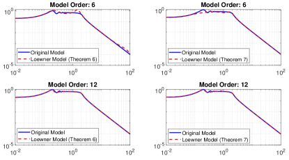
Figure 4: The Bode plots of the original model and different second-order Loewner models with orders 6 and 12 generated by the approaches in Theorems 6 and 7, respectively.

VII Conclusion

A time-domain moment matching approach for second-order dynamical systems has been presented. The moments of a given second-order system is characterized by the unique solution of a Sylvester equation, and families of parameterized reduced second-order models have been provided to match selected moments. Furthermore, we have also addressed the approaches that determine the free parameters to achieve moment matching at two distinct sets of interpolation points and matching at the first-order derivative of the transfer function of the original second-order system. Finally, we have further addressed the Loewner framework for the second-order systems, where two families of data-driven models are presented which not only interpolate the sets of tangential data but also retains the second structure from the original system.

References

• [1] B. Yan, S. X.-D. Tan, and B. McGaughy, “Second-order balanced truncation for passive-order reduction of RLCK circuits,” IEEE Transactions on Circuits and Systems II: Express Briefs, vol. 55, no. 9, pp. 942–946, 2008.
• [2] F. Dörfler, M. R. Jovanovic, M. Chertkov, and F. Bullo, “Sparsity-promoting optimal wide-area control of power networks,” IEEE Transactions on Power Systems, vol. 29, no. 5, pp. 2281–2291, 2014.
• [3] B. Safaee and S. Gugercin, “Structure-preserving model reduction of parametric power networks,” arXiv preprint arXiv:2102.05179, 2021.
• [4] F. Ma, M. Morzfeld, and A. Imam, “The decoupling of damped linear systems in free or forced vibration,” Journal of Sound and vibration, vol. 329, no. 15, pp. 3182–3202, 2010.
• [5] P. Koutsovasilis and M. Beitelschmidt, “Comparison of model reduction techniques for large mechanical systems,” Multibody System Dynamics, vol. 20, no. 2, pp. 111–128, 2008.
• [6] D. G. Meyer and S. Srinivasan, “Balancing and model reduction for second-order form linear systems,” IEEE Transactions on Automatic Control, vol. 41, no. 11, pp. 1632–1644, 1996.
• [7] Y. Chahlaoui, D. Lemonnier, A. Vandendorpe, and P. Van Dooren, “Second-order balanced truncation,” Linear Algebra and its Applications, vol. 415, no. 2, pp. 373–384, 2006.
• [8] T. Reis and T. Stykel, “Balanced truncation model reduction of second-order systems,” Mathematical and Computer Modelling of Dynamical Systems, vol. 14, no. 5, pp. 391–406, 2008.
• [9] P. Benner and J. Saak, “Efficient balancing-based MOR for large-scale second-order systems,” Mathematical and Computer Modelling of Dynamical Systems, vol. 17, no. 2, pp. 123–143, 2011.
• [10] P. Benner, P. Kürschner, and J. Saak, “An improved numerical method for balanced truncation for symmetric second-order systems,” Mathematical and Computer Modelling of Dynamical Systems, vol. 19, no. 6, pp. 593–615, 2013.
• [11] C. Hartmann, V.-M. Vulcanov, and C. Schütte, “Balanced truncation of linear second-order systems: a hamiltonian approach,” Multiscale Modeling & Simulation, vol. 8, no. 4, pp. 1348–1367, 2010.
• [12] I. Dorschky, T. Reis, and M. Voigt, “Balanced truncation model reduction for symmetric second order systems–a passivity-based approach,” arXiv preprint arXiv:2006.09170, 2020.
• [13] K. Sato, “Riemannian optimal model reduction of linear second-order systems,” IEEE control systems letters, vol. 1, no. 1, pp. 2–7, 2017.
• [14] L. Yu, X. Cheng, J. Scherpen, and J. Xiong, “$H_{2}$ model reduction for diffusively coupled second-order networks by convex-optimization,” arXiv preprint arXiv:2104.04321, 2021.
• [15] X. Cheng, Y. Kawano, and J. M. A. Scherpen, “Reduction of second-order network systems with structure preservation,” IEEE Transactions on Automatic Control, vol. 62, pp. 5026 – 5038, 2017.
• [16] X. Cheng and J. M. A. Scherpen, “Clustering approach to model order reduction of power networks with distributed controllers,” Advances in Computational Mathematics, vol. 44, no. 6, pp. 1917–1939, Dec 2018.
• [17] T. Ishizaki and J.-i. Imura, “Clustered model reduction of interconnected second-order systems,” Nonlinear Theory and Its Applications, IEICE, vol. 6, no. 1, pp. 26–37, 2015.
• [18] A. C. Antoulas, Approximation of Large-Scale Dynamical Systems.   Philadelphia, USA: SIAM, 2005.
• [19] K. Gallivan, A. Vandendorpe, and P. Van Dooren, “Sylvester equations and projection-based model reduction,” Journal of Computational and Applied Mathematics, vol. 162, no. 1, pp. 213–229, 2004.
• [20] A. C. Antoulas, C. A. Beattie, and S. Gugercin, “Interpolatory model reduction of large-scale dynamical systems,” in Efficient modeling and control of large-scale systems.   Springer, 2010, pp. 3–58.
• [21] A. Astolfi, “Model reduction by moment matching for linear and nonlinear systems,” IEEE Transactions on Automatic Control, vol. 55, no. 10, pp. 2321–2336, 2010.
• [22] A. Astolfi, G. Scarciotti, J. Simard, N. Faedo, and J. V. Ringwood, “Model reduction by moment matching: Beyond linearity a review of the last 10 years,” in 2020 59th IEEE Conference on Decision and Control (CDC).   IEEE, 2020, pp. 1–16.
• [23] Z. Bai and Y. Su, “Dimension reduction of large-scale second-order dynamical systems via a second-order arnoldi method,” SIAM Journal on Scientific Computing, vol. 26, no. 5, pp. 1692–1709, 2005.
• [24] B. Salimbahrami and B. Lohmann, “Order reduction of large scale second-order systems using Krylov subspace methods,” Linear Algebra and its Applications, vol. 415, no. 2, pp. 385–405, 2006.
• [25] C. A. Beattie and S. Gugercin, “Krylov-based model reduction of second-order systems with proportional damping,” in Proceedings of the 44th IEEE Conference on Decision and Control, 2005 and 2005 European Control Conference. CDC-ECC’05.   IEEE, 2005, pp. 2278–2283.
• [26] Z.-Y. Qiu, Y.-L. Jiang, and J.-W. Yuan, “Interpolatory model order reduction method for second order systems,” Asian Journal of Control, vol. 20, no. 1, pp. 312–322, 2018.
• [27] M. Vakilzadeh, M. Eghtesad, R. Vatankhah, and M. Mahmoodi, “A krylov subspace method based on multi-moment matching for model order reduction of large-scale second order bilinear systems,” Applied Mathematical Modelling, vol. 60, pp. 739–757, 2018.
• [28] A. Astolfi, “Model reduction by moment matching, steady-state response and projections,” in Proceedings of 49th IEEE Conference on Decision and Control (CDC).   IEEE, 2010, pp. 5344–5349.
• [29] T. C. Ionescu and A. Astolfi, “Families of moment matching based, structure preserving approximations for linear port-Hamiltonian systems,” Automatica, vol. 49, no. 8, pp. 2424–2434, 2013.
• [30] T. Ionescu, “Two-sided time-domain moment matching for linear systems.” IEEE Transactions Automatic Control, vol. 61, no. 9, pp. 2632–2637, 2016.
• [31] T. C. Ionescu, A. Astolfi, and P. Colaneri, “Families of moment matching based, low order approximations for linear systems,” Systems and Control Letters, vol. 64, no. 1, pp. 47–56, 2014.
• [32] A. Astolfi, “Model reduction by moment matching for linear and nonlinear systems,” IEEE Trans. Autom. Contr., vol. 50, no. 10, pp. 2321–2336, 2010.
• [33] T. C. Ionescu, A. Astolfi, and P. Colaneri, “Families of moment matching based, low order approximations for linear systems,” Systems & Control Letters, vol. 64, pp. 47–56, 2014.
• [34] A. C. Antoulas, Approximation of large-scale dynamical systems.   Philadelphia: SIAM, 2005.
• [35] E. de Souza and S. P. Bhattacharyya, “Controllability, observability and the solution of ${AX}-{XB}={C}$,” Linear Algebra & Its App., vol. 39, pp. 167–188, 1981.
• [36] K. Gallivan, A. Vandendorpe, and P. V. Dooren, “Model reduction of MIMO systems via tangential interpolation,” SIAM J. Matrix Anal. Appl., vol. 26, no. 2, pp. 328–349, 2004.
• [37] D. S. Bernstein and S. P. Bhat, “Lyapunov stability, semistability, and asymptotic stability of matrix second-order systems,” Journal of Mechanical Design, vol. 117, no. B, pp. 145–153, 1995.
• [38] S. Datta, D. Chakraborty, and B. Chaudhuri, “Partial pole placement with controller optimization,” IEEE Transactions on Automatic Control, vol. 57, no. 4, pp. 1051–1056, 2012.
• [39] T. C. Ionescu, O. V. Iftime, and I. Necoara, “Model reduction with pole-zero placement and high order moment matching,” arXiv preprint arXiv:2003.06049, 2021.
• [40] A. J. Mayo and A. C. Antoulas, “A framework for the solution of the generalized realization problem,” Linear Algebra & Its App., vol. 425, pp. 634–662, 2007.
• [41] D. Karachalios, I. V. Gosea, and A. C. Antoulas, “The loewner framework for system identification and reduction,” in Model Order Reduction: Volume I: System-and Data-Driven Methods and Algorithms.   De Gruyter, 2021, pp. 181–228.
• [42] J. D. Simard and A. Astolfi, “Nonlinear model reduction in the loewner framework,” IEEE Transactions on Automatic Control, vol. 66, no. 12, pp. 5711–5726, 2021.
• [43] J. D. Simard, X. Cheng, and A. Moreschini, “Interpolants with second-order structure in the loewner framework,” To appear in the 22nd IFAC World Congress, 2023.
• [44] I. P. Duff, P. Goyal, and P. Benner, “Data-driven identification of rayleigh-damped second-order systems,” Realization and Model Reduction of Dynamical Systems: A Festschrift in Honor of the 70th Birthday of Thanos Antoulas, p. 255, 2019.