Characterising transformations between quantum objects, ‘completeness’ of quantum properties, and transformations without a fixed causal order

Simon Milz OrcID: 0000-0002-6987-5513 Email: MILZS@tcd.ie Affiliation: School of Physics, Trinity College Dublin, Dublin 2, Ireland Affiliation: Trinity Quantum Alliance, Unit 16, Trinity Technology and Enterprise Centre, Pearse Street, Dublin 2, D02YN67, Ireland Affiliation: Institute for Quantum Optics and Quantum Information, Austrian Academy of Sciences, Boltzmanngasse 3, 1090 Vienna, Austria Affiliation: Faculty of Physics, University of Vienna, Boltzmanngasse 5, 1090 Vienna, Austria    Marco Túlio Quintino OrcID: 0000-0003-1332-3477 Email: Marco.Quintino@lip6.fr Affiliation: Sorbonne Université, CNRS, LIP6, F-75005 Paris, France
15th July 2024
Abstract

Many fundamental and key objects in quantum mechanics are linear mappings between particular affine/linear spaces. This structure includes basic quantum elements such as states, measurements, channels, instruments, non-signalling channels and channels with memory, and also higher-order operations such as superchannels, quantum combs, n-time processes, testers, and process matrices which may not respect a definite causal order. Deducing and characterising their structural properties in terms of linear and semidefinite constraints is not only of foundational relevance, but plays an important role in enabling the numerical optimisation over sets of quantum objects and allowing simpler connections between different concepts and objects. Here, we provide a general framework to deduce these properties in a direct and easy to use way. While primarily guided by practical quantum mechanical considerations, we also extend our analysis to mappings between general linear/affine spaces and derive their properties, opening the possibility for analysing sets which are not explicitly forbidden by quantum theory, but are still not much explored. Together, these results yield versatile and readily applicable tools for all tasks that require the characterisation of linear transformations, in quantum mechanics and beyond. As an application of our methods, we discuss how the existence of indefinite causality naturally emerges in higher-order quantum transformations and provide a simple strategy for the characterisation of mappings that have to preserve properties in a ‘complete’ sense, i.e., when acting non-trivially only on parts of an input space.

1 Introduction

Many fundamental objects in quantum mechanics can, at their most basic level, be understood as (linear) transformations of other basic objects. For example, measurements are transformations of states to probabilities, while quantum channels are transformations of quantum states to quantum states. This simple understanding of quantum objects as transformations can straightforwardly be extended, leading to a whole host of higher-order transformations (see Fig. 1 for an example). To name but a few, transformations of channels to channels (yielding so-called superchannels [1]), sequences of quantum channels with memory to quantum channels (yielding so-called quantum combs [2] and quantum strategies [3]), a sequence of channels to states (yielding so-called multi-time processes [4]) and collections of channels to probabilities (yielding testers [5, 6, 7] and process matrices [8]) have been devised in recent years, each with their own respective physical motivation. On the other hand, such higher-order transformations can equivalently be motivated as the correct descriptor in many physical situations, where states, measurements and channels alone would prove to be insufficient practical tools. Consequently, they have, amongst others, found active use in the fields of open quantum system dynamics [4], quantum circuit architecture [2], the investigation of channels with memory [9], as well as the study of causal indefiniteness [8] and the dynamics of causal order [10].

Refer to caption
Figure 1: Chain of higher-order operations. A pictorial illustration of an exemplary chain of higher-order operations. Channels describe transformations between states, superchannels describe transformation between channels, and supersuperchannels describe transformations between superchannels. The methods we provide allow for the characterization of all mappings in this chain, but more generally all mappings between arbitrary quantum objects. The precise definition and a characterisation of such objects and the mappings between them can be found in Sec. 4.

Independent of the respective concrete motivation, in any of these investigations it is, as a first step, frequently necessary to deduce the structural properties of the considered transformations, i.e., a characterisation of the transformation in a chosen representation11 1 Here, and throughout, unless stated otherwise, we mean a characterisation of the Choi matrix of the transformation when we consider its ‘properties’. that goes beyond its original definition. For example, for the case of process matrices, one is interested in the structure of mappings that map pairs of independent quantum channels (or, equivalently, any two-party non-signalling channel) to unit probability, in order to analyse the set of processes that abide by causality locally, but not necessarily globally [8]. Having their at hand then does not only allow one to deduce that this latter set fundamentally differs from the set of causally ordered processes, but also enables numerical optimisation over causally indefinite processes. On the more axiomatic side, recent works have discussed the properties of the hierarchy of transformations that emerges from starting at quantum states and ’going up the ladder’ of transformations, i.e., transformations of states, transformations of transformations of states, etc. [11, 12, 13, 14].

Here, we stay agnostic with respect to the origin of the respective transformations and provide a general framework to answer the question: What are the properties of linear transformations between affine/linear spaces? For example, this question directly captures the case of quantum channels – completely positive mappings of the affine space of matrices with unit trace onto itself – but also all conceivable transformations between quantum objects alluded to before. Concretely, we phrase the properties of the respective spaces as well as the transformations between them in terms of linear projectors and employ their representation as matrices via the Choi isomorphism for their explicit characterisation. The ’projector approach’ and the methods presented here may be viewed as deeper analysis and a generalisation of the ideas first presented in Ref. [15], which were developed to present a basis-independent characterisation for process matrices and to study quantum processes which do not respect a definite causal order. A similar approach to the characterisation of higher-order maps has, for example, been taken in [10, 16, 14, 13]. Moreover, in-depth investigations into the structure and type theory of the hierarchy of conceivable higher-order quantum maps can be found in Refs. [11, 12, 14, 13, 17], where, in particular Ref. [14] not only employs a similar approach to ours, but also provides a detailed analysis of the logical and set-theoretic structure of the projectors that define the properties of the transformations we analyse.

This current work is more modest in scope; leveraging the link product [5] and the linearity of the involved transformations, we provide a straightforward, systematic way to derive the properties of arbitrary transformations between sets that naturally emerge in quantum mechanics. In turn, this allows us to re-derive the properties of a vast array of relevant quantum transformations appearing in different parts of the literature in a unified and direct way. We further demonstrate the effectiveness and ease of this framework by explicitly discussing affine dual sets as well as probabilistic quantum operations and the signalling structures of quantum maps. As an additional application of our methods, we analyse the emergence of indefinite causal order in higher-order quantum operations.

In many cases of interest, a transformation does not only have to preserve certain properties (like, for example, the trace of a state) when acting entirely on the input space, but also when acting non-trivially on only a part of it. This is the reasoning behind the introduction of complete positivity (in contrast to mere positivity), which requires not only positivity of a map C~\widetilde{C}, but also positivity of all of its trivial extensions C~𝟙~\widetilde{C}\otimes\widetilde{\mathds{1}}, where 𝟙~\widetilde{\mathds{1}} is the identity map on an arbitrary anciliary space. While most commonly encountered in the context of positivity and complete positivity, the analogous question can equivalently be raised for other properties of quantum transformations. For example, it is obvious that C~𝟙~\widetilde{C}\otimes\widetilde{\mathds{1}} is trace preserving if C~\widetilde{C} is, but it is a priori unclear if ‘completeness’ of properties is automatically implied for more general properties. Even more so, for many relevant cases, it not even immediate or unique, how a specific property should be extended to a larger input space. Parts of this question have – in different contexts – been considered in the literature, either for concrete questions at hand [18, 19, 16], or for specific types of extensions [13, 14, 20, 21]. Here, using the characterisation of quantum transformations, we provide a simple strategy to derive the structure of transformations that have to preserve a structural property in a ‘complete’ sense. In particular, this approach is agnostic to the chosen extension, and allows for the identification of sufficient conditions under which a transformation is automatically completely admissible. The versatility and applicability of this approach is then demonstrated by means of concrete examples, that not only recover known cases from the literature, but also demonstrate how the requirements imposed by ‘completeness’ fundamentally depend on the chosen extension of a property.

Finally, owing to the simplicity of our approach, we are also able to drop the assumptions generally fulfilled in quantum mechanics – like, for example, the self-adjointness of the involved projectors, or the membership of the identity matrix to the respective input and output spaces – and derive the properties of transformation between general spaces, a result that might be of interest in its own right. Together, our results provide a unified framework to discuss and characterise all (quantum) objects and linear transformations thereof as well as the restrictions imposed by ‘completeness’, thus offering a versatile tool for a wide array of problems that naturally occur in the field of quantum mechanics in beyond.

2 Warming up: quantum states and quantum channels

The fundamental set of objects that quantum mechanics is concerned with are quantum states ρ()\rho\in\mathcal{L}(\mathcal{H}), unit trace (i.e., tr[ρ]=1\tr[\rho]=1), positive semidefinite (i.e., ρ0\rho\geq 0) linear operators acting on a Hilbert space \mathcal{H}. Here, and throughout, we consider \mathcal{H} to be finite dimensional, such that d\mathcal{H}\cong\mathbb{C}^{d} for some dd\in\mathbb{N}.

Transformations of quantum states are then described by linear maps T~:(i)(o)\widetilde{T}:\mathcal{L}(\mathcal{H}_{\textup{{i}}})\to\mathcal{L}(\mathcal{H}_{\textup{{o}}}), where we adopt the convention of referring to the input space as i\mathcal{H}_{\textup{{i}}}, the output space as o\mathcal{H}_{\textup{{o}}} and maps between operators with a tilde. For better bookkeeping, we always explicitly distinguish between input and output spaces, even if io\mathcal{H}_{\textup{{i}}}\cong\mathcal{H}_{\textup{{o}}}.22 2 The only exception to this rule will be the projectors P~\widetilde{P} that we introduce below. A transformation T~\widetilde{T} is a valid quantum channel, i.e., it represents a deterministic transformation between quantum states that can be physically implemented, if it is a completely positive (CP)33 3 A linear map T~:(i)(o)\widetilde{T}:\mathcal{L}(\mathcal{H}_{\textup{{i}}})\to\mathcal{L}(\mathcal{H}_{\textup{{o}}}) is positive when T~[ρ]0\widetilde{T}[\rho]\geq 0 for every positive semidefinite linear operator ρ0,ρ(i)\rho\geq 0,\rho\in\mathcal{L}(\mathcal{H}_{\textup{{i}}}). A map is CP if it is positive for all trivial extensions, that is, T~𝟙~(σ)0\widetilde{T}\otimes\widetilde{\mathds{1}}(\sigma)\geq 0 for every positive semidefinite σ(iaux){\sigma\in\mathcal{L}(\mathcal{H}_{\textup{{i}}}\otimes\mathcal{H}_{\text{aux}})} where 𝟙~:(aux)(aux)\widetilde{\mathds{1}}:\mathcal{L}(\mathcal{H}_{\text{aux}})\to\mathcal{L}(\mathcal{H}_{\text{aux}}) is the identity map on an arbitrary finite space aux\mathcal{H}_{\text{aux}}, i.e., 𝟙~[ρ]=ρ,ρ(aux)\widetilde{\mathds{1}}[\rho]=\rho,\forall\rho\in\mathcal{L}(\mathcal{H}_{\text{aux}}). and trace-preserving44 4 A linear map T~:(i)(o)\widetilde{T}:\mathcal{L}(\mathcal{H}_{\textup{{i}}})\to\mathcal{L}(\mathcal{H}_{\textup{{o}}}) is TP when tr[T~[ρ]]=tr[ρ]\tr[\widetilde{T}[\rho]]=\tr[\rho] for every linear operator ρ(i)\rho\in\mathcal{L}(\mathcal{H}_{\textup{{i}}}). (TP) linear map.

While the mathematical characterisation of matrices that represent quantum states ρ\rho is clear, it is, a priori, unclear, what the corresponding properties of a representation of a quantum channel – a transformation between sets of quantum states – are. Here, we aim to provide a simple way of characterising mappings between objects that routinely occur in quantum mechanics. To illustrate the general concept, we first provide an answer for the well-known case of CPTP maps. To this end, we exploit the fact that linear maps admit a convenient representation as linear operators via the Choi-Jamiołkowski isomorphism (CJI) [22, 23, 24]: Let {|j}j\{|j\rangle\}_{j} be the canonical computational basis for i\mathcal{H}_{\textup{{i}}}. The Choi operator/matrix T(io)T\in\mathcal{L}(\mathcal{H}_{\textup{{i}}}\otimes\mathcal{H}_{\textup{{o}}}) of a linear map T~:(i)(o)\widetilde{T}:\mathcal{L}(\mathcal{H}_{\textup{{i}}})\to\mathcal{L}(\mathcal{H}_{\textup{{o}}}) is then defined as

T:=jk|jk|T~[|jk|].T:=\sum_{jk}|j\rangle\hskip-1.13809pt\langle k|\otimes\widetilde{T}\big[|j\rangle\hskip-1.13809pt\langle k|\big]. (1)

Direct calculation shows that the action of T~\widetilde{T} can be written in terms of its Choi matrix TT as

T~[ρ]=tri[(ρτ𝟙o)T]\widetilde{T}[\rho]=\tr_{\textup{{i}}}[(\rho^{\tau}\otimes\mathds{1}_{\textup{{o}}})\;T] (2)

where ρτ\rho^{\tau} is the transpose of ρ\rho in the computational basis and tri\tr_{\textup{{i}}} is the partial trace over i\mathcal{H}_{\textup{{i}}}.

(a)
(b)
Figure 2: Quantum states and Quantum Channels. (a) Quantum state ρ(i)\rho\in\mathcal{L}(\mathcal{H}_{\textup{{i}}}). (b) Quantum channel C~:(i)(o)\widetilde{C}:\mathcal{L}(\mathcal{H}_{\textup{{i}}})\rightarrow\mathcal{L}(\mathcal{H}_{\textup{{o}}}) that maps quantum states in (i)\mathcal{L}(\mathcal{H}_{\textup{{i}}}) onto quantum states in (o)\mathcal{L}(\mathcal{H}_{\textup{{o}}}). Throughout, lines are labelled by the Hilbert space/space of linear operators they correspond to.

To characterise the properties of TT, we note that a linear map T~:(i)(o)\widetilde{T}:\mathcal{L}(\mathcal{H}_{\textup{{i}}})\to\mathcal{L}(\mathcal{H}_{\textup{{o}}}) is TP if and only if, tro[T]=𝟙i\tr_{\textup{{o}}}[T]=\mathds{1}_{\textup{{i}}} and CP if and only if T0T\geq 0. Hence, CPTP maps (quantum channels) C~\widetilde{C} are described by a Choi matrix C(io)C\in\mathcal{L}(\mathcal{H}_{\textup{{i}}}\otimes\mathcal{H}_{\textup{{o}}}) that satisfies

C\displaystyle C\geq 0andtro[C]=𝟙i.\displaystyle 0\quad\text{and}\quad\tr_{\textup{{o}}}[C]=\mathds{1}_{\textup{{i}}}. (3)

In anticipation of later considerations, we can phrase this equivalently as

C\displaystyle C\geq 0\displaystyle 0 (4)
Co=\displaystyle{}_{\textup{{o}}}C= Cio{}_{\textup{{i}}\textup{{o}}}C (5)
tr[C]=\displaystyle\tr[C]= di,\displaystyle d_{\textup{{i}}}, (6)

where Cx:=trx[C]𝟙xdx{}_{\texttt{x}}C:=\tr_{\texttt{x}}[C]\otimes\frac{\mathds{1}_{\texttt{x}}}{d_{\texttt{x}}} is the trace-and-replace map and dxd_{\texttt{x}} is the dimension of x\mathcal{H}_{\texttt{x}}. Notice that, for consistency, one should keep track of the ordering of the operators, for instance, if C(io)C\in\mathcal{L}(\mathcal{H}_{\textup{{i}}}\otimes\mathcal{H}_{\textup{{o}}}), Ci=𝟙iditri[C]{}_{\textup{{i}}}C=\frac{\mathds{1}_{\textup{{i}}}}{d_{\textup{{i}}}}\otimes\tr_{\textup{{i}}}[C] and Co=tro[C]𝟙odo{}_{\textup{{o}}}C=\tr_{\textup{{o}}}[C]\otimes\frac{\mathds{1}_{\textup{{o}}}}{d_{\textup{{o}}}}. Whenever there is risk of ambiguity, or we desire to emphasise some property, we will use subscripts (rather than explicit ordering) to indicate what space an object is defined/acts on.

The characterisation of quantum channels given by Eqs. (4)– (6) has an interesting structure, which will be the starting point to analyse the structure of more general transformations throughout this work. Eq. (4) is a positivity constraint, Eq. (5) is a linear constraint, and Eq. (6) is an affine constraint. Consequently, the set of linear operators satisfying Eq. (5) form a linear subspace of (io)\mathcal{L}(\mathcal{H}_{\textup{{i}}}\otimes\mathcal{H}_{\textup{{o}}}), and can thus be described by a projective map P~:(io)(io)\widetilde{P}:\mathcal{L}(\mathcal{H}_{\textup{{i}}}\otimes\mathcal{H}_{\textup{{o}}})\to\mathcal{L}(\mathcal{H}_{\textup{{i}}}\otimes\mathcal{H}_{\textup{{o}}}), where

Co=CioC=P~[C]withP~[C]:=CCo+Cio.{}_{\textup{{o}}}C={}_{\textup{{i}}\textup{{o}}}C\iff C=\widetilde{P}[C]\quad\text{with}\quad\widetilde{P}[C]:=C-{}_{\textup{{o}}}C+{}_{\textup{{i}}\textup{{o}}}C\,. (7)

We can easily verify that P~\widetilde{P} is indeed a projective map, that is, P~2:=P~P~=P~{\widetilde{P}}^{2}:=\widetilde{P}\circ\widetilde{P}=\widetilde{P}. Putting everything together, an operator C(12)C\in\mathcal{L}(\mathcal{H}_{1}\otimes\mathcal{H}_{2}) is the Choi operator of a quantum channel if and only if

C\displaystyle C 0,\displaystyle\geq 0,\quad\qquad (Positive semidefinite) (8)
C\displaystyle C =P~[C],\displaystyle=\widetilde{P}[C], (Linear subspace) (9)
tr[C]\displaystyle\tr[C] =di,\displaystyle=d_{\textup{{i}}}, (Fixed trace).\displaystyle\text{(Fixed trace)}. (10)

Put differently, besides the positivity and overall trace constraint, the set of quantum channels is fully defined by the projector P~\widetilde{P}.

While positivity of the Choi matrix simply follows from the requirement of complete positivity for the map (a property that we will assume throughout), for more general mappings, working out both the trace constraint and the correct projector can be somewhat cumbersome. For example, it is a priori unclear what properties a mapping from quantum channels to quantum channels (a so-called supermap [1] or superchannel) would possess, and similar for any mapping ‘higher up in the hierarchy’. Below, we extend the above concepts and methods to provide a direct and systematic way to derive the linear and affine constraints for transformations between general quantum objects (see Fig. 3 for a graphical depiction).

Refer to caption
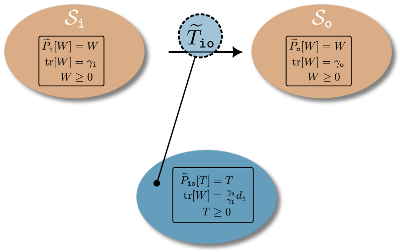
Figure 3: General Transformations between affine (quantum) sets All sets 𝒮i\mathcal{S}_{\textup{{i}}} and 𝒮o\mathcal{S}_{\textup{{o}}} we consider are defined by a linear constraint (given by P~i\widetilde{P}_{\textup{{i}}} and P~o\widetilde{P}_{\textup{{o}}}, respectively) and in most cases an affine and a positivity constraint. Our aim is to characterise the set of linear transformations T~io\widetilde{T}_{\textup{{i}}\textup{{o}}} between them. Predominantly, this characterisation will be carried out for the Choi matrices TT of said transformations, and as it turns out, the corresponding set of matrices is, again, defined by a projector P~io\widetilde{P}_{\textup{{i}}\textup{{o}}}, as well as an affine and a positivity constraint. The concrete construction of P~io\widetilde{P}_{\textup{{i}}\textup{{o}}} depends on the respective properties of P~i\widetilde{P}_{\textup{{i}}} and P~o\widetilde{P}_{\textup{{o}}}. Thm. 2 provides this construction for the special case most often encountered in quantum mechanics, while the general case is discussed in Thm. 5. Likewise, the case where there are no affine constraints on 𝒮i\mathcal{S}_{\textup{{i}}} and 𝒮o\mathcal{S}_{\textup{{o}}} is discussed in Thms. 4 and 6.

3 Linear transformations between quantum objects

3.1 Sets of quantum objects

The characterisation (7) of the set of quantum channels via a projector provides a potent way to derive the structural properties of mappings that occur frequently in quantum mechanics. We can use this structure to represent a very general class of (deterministic) quantum objects, such as quantum states, quantum channels, quantum superchannel [1], quantum combs [2, 5], channels with memory [9], quantum strategies [3], non-Markovian processes [25], causal quantum operations [26], non-signalling channels [27], process matrices [8, 15], and more generally mappings between any kinds of linear spaces [11, 12, 13, 14, 17]. Before discussing the fully general case, i.e., mappings between general linear spaces (see Sec. 9), we start with a discussion of scenarios that are commonly encountered in quantum mechanics.

Definition 1 (Set of quantum objects).

A set of linear operators 𝒮()\mathcal{S}\subseteq\mathcal{L}(\mathcal{H}) is a quantum object set if it can be described by:

A linear operator W\displaystyle\text{A linear operator }W ()\displaystyle\in\mathcal{L}(\mathcal{H}) belongs to 𝒮\mathcal{S} if and only if:
W\displaystyle W 0\displaystyle\geq 0 (Positive semidefinite), (11a)
P~[W]\displaystyle\widetilde{P}[W] =W\displaystyle=W (Belongs to a particular linear subspace), (11b)
tr[W]\displaystyle\tr[W] =γ\displaystyle=\gamma (Fixed trace),\displaystyle\text{(Fixed trace)}, (11c)

where P~:()()\widetilde{P}:\mathcal{L}(\mathcal{H})\to\mathcal{L}(\mathcal{H}) is a linear projective map, that is P~2:=P~P~=P~\widetilde{P}^{2}:=\widetilde{P}\circ\widetilde{P}=\widetilde{P}.

For example, both quantum states and the set of Choi matrices of quantum channels satisfy the above definition. For quantum states, we have P~=𝟙~\widetilde{P}=\widetilde{\mathds{1}} (where 𝟙~\widetilde{\mathds{1}} denotes the identity map55 5 The identity map is defined by 𝟙~[X]=X\widetilde{\mathds{1}}[X]=X for all X()X\in\mathcal{L}(\mathcal{H}).) and γ=1\gamma=1, while for quantum channels, P~\widetilde{P} is given by Eq. (7) and γ=di\gamma=d_{\textup{{i}}}.

3.2 Transformations between quantum objects

Let us consider two arbitrary sets of quantum objects 𝒮i(i)\mathcal{S}_{\textup{{i}}}\subseteq\mathcal{L}(\mathcal{H}_{\textup{{i}}}) and 𝒮o(o)\mathcal{S}_{\textup{{o}}}\subseteq\mathcal{L}(\mathcal{H}_{\textup{{o}}}) where we use i  and o  as general placeholders for ’input’ and ’output’. Our main question then is:

How can the set of quantum transformations T~io\widetilde{T}_{\textup{{i}}\textup{{o}}} from 𝒮i\mathcal{S}_{\textup{{{i}}}} to 𝒮o\mathcal{S}_{\textup{{{o}}}} be characterised?

Since we require T~io\widetilde{T}_{\textup{{i}}\textup{{o}}} to map elements from 𝒮i\mathcal{S}_{\textup{{{i}}}} to 𝒮o\mathcal{S}_{\textup{{{o}}}}, we require that for every W𝒮iW\in\mathcal{S}_{\textup{{i}}}, we have that T~io[W]𝒮o\widetilde{T}_{\textup{{i}}\textup{{o}}}[W]\in\mathcal{S}_{\textup{{o}}}, where we use additional subscripts on T~\widetilde{T} to signify its input and output space. Also, in order to be consistent with the linearity of quantum theory, the transformation T~io\widetilde{T}_{\textup{{i}}\textup{{o}}} is required to be a linear map from the linear space spanned by 𝒮i\mathcal{S}_{\textup{{i}}} to the linear space spanned by 𝒮o\mathcal{S}_{\textup{{o}}}. Additionally, since all elements of 𝒮i\mathcal{S}_{\textup{{i}}} and 𝒮o\mathcal{S}_{\textup{{o}}} are positive, we would at least require that T~io\widetilde{T}_{\textup{{i}}\textup{{o}}} is positive on all W𝒮iW\in\mathcal{S}_{\textup{{i}}}. In line with standard considerations in quantum mechanics, throughout, we go beyond this minimal requirement66 6 Positivity can also be argued for in order to ensure that all probabilistic quantum object (see Sec. 6 for more details) are mapped to positive objects as well. However, this argument requires that the probabilistic quantum objects, i.e., all W(i)W^{\sharp}\in\mathcal{L}(\mathcal{H}_{\textup{{i}}}) which satisfy WWW^{\sharp}\leq W for some W𝒮iW\in\mathcal{S}_{\textup{{i}}}, span the full space (i)\mathcal{L}(\mathcal{H}_{\textup{{i}}}). This is the case if 𝒮i\mathcal{S}_{i} contains at least one full rank state, which we generally assume (see below). and demand that T~io\widetilde{T}_{\textup{{i}}\textup{{o}}} is a positive map on all of (i)\mathcal{L}(\mathcal{H}_{\textup{{i}}}). Finally, similarly to quantum channels acting on quantum states, we desire T~io\widetilde{T}_{\textup{{i}}\textup{{o}}} to be a valid transformation even when it is applied to only a part of a larger quantum object, which (at least) requires that T~io:(i)(o)\widetilde{T}_{\textup{{i}}\textup{{o}}}:\mathcal{L}(\mathcal{H}_{\textup{{i}}})\to\mathcal{L}(\mathcal{H}_{\textup{{o}}}) is completely positive. In turn, this implies that all Choi matrices we encounter throughout are positive semidefinite (see Sec. 3.4).

Definition 2 (Quantum Transformations).

Let P~i:(i)(i)\widetilde{P}_{\textup{{i}}}:\mathcal{L}(\mathcal{H}_{\textup{{i}}})\to\mathcal{L}(\mathcal{H}_{\textup{{i}}}) and P~o:(o)(o)\widetilde{P}_{\textup{{o}}}:\mathcal{L}(\mathcal{H}_{\textup{{o}}})\to\mathcal{L}(\mathcal{H}_{\textup{{o}}}) be linear projective maps and 𝒮i(i)\mathcal{S}_{\textup{{i}}}\subseteq\mathcal{L}(\mathcal{H}_{\textup{{i}}}) and 𝒮o(o)\mathcal{S}_{\textup{{o}}}\subseteq\mathcal{L}(\mathcal{H}_{\textup{{o}}}) be sets of quantum objects defined by

W(i)W\in\mathcal{L}(\mathcal{H}_{\textup{{i}}}) belongs to 𝒮i\mathcal{S}_{\textup{{i}}} iff W(o)W^{\prime}\in\mathcal{L}(\mathcal{H}_{\textup{{o}}}) belongs to 𝒮o\mathcal{S}_{\textup{{o}}} iff
W0W\geq 0,     \mathbf{\longrightarrow} W0W^{\prime}\geq 0,
P~i[W]=W\widetilde{P}_{\textup{{i}}}[W]=W, P~o[W]=W\widetilde{P}_{\textup{{o}}}[W^{\prime}]=W^{\prime},
tr[W]=γi\tr[W]=\gamma_{\textup{{i}}}. tr[W]=γo\tr[W^{\prime}]=\gamma_{\textup{{o}}}.

A linear map T~io:(i)(o)\widetilde{T}_{\textup{{i}}\textup{{o}}}:\mathcal{L}(\mathcal{H}_{\textup{{i}}})\to\mathcal{L}(\mathcal{H}_{\textup{{o}}}) is a quantum transformation from 𝒮i\mathcal{S}_{\textup{{i}}} to 𝒮o\mathcal{S}_{\textup{{o}}} if:

i:\displaystyle i: T~io is completely positive\displaystyle\quad\widetilde{T}_{\textup{{i}}\textup{{o}}}\text{ is completely positive } (16a)
ii:\displaystyle ii: W𝒮i, we have that T~io[W]𝒮o\displaystyle\quad\forall W\in\mathcal{S}_{\textup{{i}}},\text{ we have that }\widetilde{T}_{\textup{{i}}\textup{{o}}}[W]\in\mathcal{S}_{\textup{{o}}} (16b)

General linear mappings of this type have previously been employed in the quantum information literature, for example for the analysis of the dynamics of quantum causal structures [10] as well as, under the guise of ’admissible adapters’, in the resource theory of causal connection [16], or as ’structure-preserving maps’ [14], in the study of transformations between general quantum objects. More detailed structural investigations of the hierarchy of transformations such maps engender have been carried out in [11, 12, 13, 14].

Importantly, for the concrete characterisation of T~io\widetilde{T}_{\textup{{i}}\textup{{o}}} (or, equivalently, its Choi matrix TioT_{\textup{{i}}\textup{{o}}}) only the linear and affine constraints on 𝒮i\mathcal{S}_{\textup{{i}}} and 𝒮o\mathcal{S}_{\textup{{o}}} play a role. The positive semidefiniteness constraint on both sets on the other hand only enters in the requirement for T~io\widetilde{T}_{\textup{{i}}\textup{{o}}} to be CP (or, equivalently, its Choi matrix TioT_{\textup{{i}}\textup{{o}}} to be positive semidefinite). Concretely, this holds true, since in the cases we consider, the positivity restriction does not alter the span of the sets, i.e., both 𝒮i\mathcal{S}_{\textup{{i}}} and 𝒮o\mathcal{S}_{\textup{{o}}} span the same spaces (P~i[(i)]\widetilde{P}_{\textup{{i}}}[\mathcal{L}(\mathcal{H}_{\textup{{i}}})] and P~o[(o)]\widetilde{P}_{\textup{{o}}}[\mathcal{L}(\mathcal{H}_{\textup{{o}}})], respectively) with or without the positivity constraints imposed on their elements. Consequently, positivity of the respective elements does not enter as an additional constraint on T~io\widetilde{T}_{\textup{{i}}\textup{{o}}}. As a result, in what follows, we rarely ever explicitly assume positivity for the elements of 𝒮i\mathcal{S}_{\textup{{i}}} and 𝒮o\mathcal{S}_{\textup{{o}}} and mostly consider transformations between affine sets. Positivity of the respective elements, as well as complete positivity of the maps between 𝒮i\mathcal{S}_{\textup{{i}}} and 𝒮o\mathcal{S}_{\textup{{o}}} can then always be imposed by hand without any added complications. On the other hand, while a similar argument could seemingly be made for the affine constraints – since they generally do not change the span of 𝒮i\mathcal{S}_{\textup{{i}}} and 𝒮o\mathcal{S}_{\textup{{o}}}, either – they fix a rescaling factor, in the sense that tr[T~io[W]]=γo/γitr[W]\tr[\widetilde{T}_{\textup{{i}}\textup{{o}}}[W]]=\gamma_{\textup{{o}}}/\gamma_{\textup{{i}}}\tr[W] for all W𝒮iW\in\mathcal{S}_{\textup{{i}}}, thus playing a crucial role for the specific properties of T~io\widetilde{T}_{\textup{{i}}\textup{{o}}}.

3.3 Map characterisation of quantum transformations

We now present our first theorem – which has, in slightly different form, already been derived in Refs. [10, 16, 13, 14] – to characterise quantum transformations. In this first characterisation, we aim to completely characterise the linear map T~io\widetilde{T}_{\textup{{i}}\textup{{o}}} without making reference to its Choi operator, but directly to its map properties.

Theorem 1 (Transformation between affine sets: map version).

Let P~i:(i)(i)\widetilde{P}_{\textup{{i}}}:\mathcal{L}(\mathcal{H}_{\textup{{i}}})\to\mathcal{L}(\mathcal{H}_{\textup{{i}}}) and P~o:(o)(o)\widetilde{P}_{\textup{{o}}}:\mathcal{L}(\mathcal{H}_{\textup{{o}}})\to\mathcal{L}(\mathcal{H}_{\textup{{o}}}) be linear projective maps and 𝒮i(i)\mathcal{S}_{\textup{{i}}}\subseteq\mathcal{L}(\mathcal{H}_{\textup{{i}}}) and 𝒮o(o)\mathcal{S}_{\textup{{o}}}\subseteq\mathcal{L}(\mathcal{H}_{\textup{{o}}}) be affine sets defined by

W(i)W\in\mathcal{L}(\mathcal{H}_{\textup{{i}}}) belongs to 𝒮i\mathcal{S}_{\textup{{i}}} iff W(o)W^{\prime}\in\mathcal{L}(\mathcal{H}_{\textup{{o}}}) belongs to 𝒮o\mathcal{S}_{\textup{{o}}} iff
P~i[W]=W\widetilde{P}_{\textup{{i}}}[W]=W,     \mathbf{\longrightarrow} P~o[W]=W\widetilde{P}_{\textup{{o}}}[W^{\prime}]=W^{\prime},
tr[W]=γi\tr[W]=\gamma_{\textup{{i}}}. tr[W]=γo\tr[W^{\prime}]=\gamma_{\textup{{o}}}.

For γi0\gamma_{\textup{{i}}}\neq 077 7 We emphasise that assuming that tr[W]0\tr[W]\neq 0 is not a strong restriction, and is quite natural for practical applications. Since all quantum objects are positive semidefinite, the only traceless object is the zero operator. In Sec. 9 we discuss a more general version of this theorem., a linear map T~io:(i)(o)\widetilde{T}_{\textup{{{i}}{{o}}}}:\mathcal{L}(\mathcal{H}_{\textup{{{i}}}})\rightarrow\mathcal{L}(\mathcal{H}_{\textup{{{o}}}}) satisfies T~io[W]𝒮o,\widetilde{T}_{\textup{{{i}}{{o}}}}[W]\in\mathcal{S}_{\textup{{{o}}}}, for all W𝒮iW\in\mathcal{S}_{\textup{{{i}}}} iff

P~oT~ioP~i\displaystyle\widetilde{P}_{\textup{{{o}}}}\circ\widetilde{T}_{\textup{{{i}}{{o}}}}\circ\widetilde{P}_{\textup{{{i}}}} =T~ioP~i,\displaystyle=\widetilde{T}_{\textup{{{i}}{{o}}}}\circ\widetilde{P}_{\textup{{{i}}}}, (20a)
andtrT~ioP~i\displaystyle\text{and}\quad\tr\circ\widetilde{T}_{\textup{{{i}}{{o}}}}\circ\widetilde{P}_{\textup{{{i}}}} =γoγitrP~i.\displaystyle=\frac{\gamma_{\textup{{o}}}}{\gamma_{\textup{{i}}}}\tr\circ\widetilde{P}_{\textup{{{i}}}}\,. (20b)
Proof.

We start by showing that if Eqs. (20a) and (20b) hold, then T~io[W]𝒮o,\widetilde{T}_{\textup{{{i}}{{o}}}}[W]\in\mathcal{S}_{\textup{{{o}}}}, for all W𝒮iW\in\mathcal{S}_{\textup{{{i}}}}. Let W𝒮iW\in\mathcal{S}_{\textup{{i}}}. Then, by definition, we have P~i[W]=W\widetilde{P}_{\textup{{i}}}[W]=W. Now, since Eq. (20a) holds, for all W𝒮iW\in\mathcal{S}_{\textup{{i}}} we have

P~o[T~io[W]]=P~oT~ioP~i[W]=T~ioP~i[W]=T~io[W].\displaystyle\widetilde{P}_{\textup{{{o}}}}[\widetilde{T}_{\textup{{{i}}{{o}}}}[W]]=\widetilde{P}_{\textup{{{o}}}}\circ\widetilde{T}_{\textup{{{i}}{{o}}}}\circ\widetilde{P}_{\textup{{{i}}}}[W]=\widetilde{T}_{\textup{{{i}}{{o}}}}\circ\widetilde{P}_{\textup{{{i}}}}[W]=\widetilde{T}_{\textup{{{i}}{{o}}}}[W]. (21)

Additionally, since tr[W]=γi\tr[W]=\gamma_{\textup{{i}}} for every W𝒮iW\in\mathcal{S}_{\textup{{i}}}, from Eq. (20b) we obtain

trT~io[W]=trT~ioP~i[W]=γoγitr[W]=γo,\displaystyle\tr\circ\widetilde{T}_{\textup{{{i}}{{o}}}}[W]=\tr\circ\widetilde{T}_{\textup{{{i}}{{o}}}}\circ\widetilde{P}_{\textup{{i}}}[W]=\frac{\gamma_{\textup{{o}}}}{\gamma_{\textup{{i}}}}\tr[W]=\gamma_{\textup{{o}}}, (22)

and hence, Eqs. (20a) and (20b) together imply that T~io[W]𝒮o,\widetilde{T}_{\textup{{{i}}{{o}}}}[W]\in\mathcal{S}_{\textup{{{o}}}}, for all W𝒮iW\in\mathcal{S}_{\textup{{{i}}}}.

For the converse direction, we note that since γi0\gamma_{\textup{{i}}}\neq 0, the affine constraint has no influence on the span of 𝒮i\mathcal{S}_{\textup{{i}}}, such that span(𝒮i)=P~i[(i)]\text{span}(\mathcal{S}_{\textup{{i}}})=\widetilde{P}_{\textup{{i}}}[\mathcal{L}(\mathcal{H}_{\textup{{i}}})]. By assumption, P~oT~io[W]=T~io[W]\widetilde{P}_{\textup{{o}}}\circ\widetilde{T}_{\textup{{i}}\textup{{o}}}[W]=\widetilde{T}_{\textup{{i}}\textup{{o}}}[W] holds for all W𝒮iW\in\mathcal{S}_{\textup{{i}}}, and by linearity, we have P~oT~io[M]=T~io[M]\widetilde{P}_{\textup{{o}}}\circ\widetilde{T}_{\textup{{i}}\textup{{o}}}[M]=\widetilde{T}_{\textup{{i}}\textup{{o}}}[M] for all Mspan(𝒮i)M\in\text{span}(\mathcal{S}_{\textup{{i}}}). For any arbitrary X(i)X\in\mathcal{L}(\mathcal{H}_{\textup{{i}}}) we have M:=P~i[X]span(𝒮i)M:=\widetilde{P}_{\textup{{i}}}[X]\in\text{span}(\mathcal{S}_{\textup{{i}}}), and thus

P~oT~ioP~i[X]=T~ioP~i[X].\displaystyle\widetilde{P}_{\textup{{o}}}\circ\widetilde{T}_{\textup{{i}}\textup{{o}}}\circ\widetilde{P}_{\textup{{i}}}[X]=\widetilde{T}_{\textup{{i}}\textup{{o}}}\circ\widetilde{P}_{\textup{{i}}}[X]. (23)

Since this holds for arbitrary X(i)X\in\mathcal{L}(\mathcal{H}_{\textup{{i}}}), we see that Eq. (20a) is satisfied. Similarly, if T~io\widetilde{T}_{\textup{{i}}\textup{{o}}} is a map from 𝒮i\mathcal{S}_{\textup{{i}}} to 𝒮o\mathcal{S}_{\textup{{o}}}, by linearity, we see that tr[T~io[M]]=γo/γitr[M]\tr[\widetilde{T}_{\textup{{i}}\textup{{o}}}[M]]=\gamma_{\textup{{o}}}/\gamma_{\textup{{i}}}\tr[M] for all Mspan(𝒮i)M\in\text{span}(\mathcal{S}_{\textup{{i}}}). Thus, for arbitrary X(i)X\in\mathcal{L}(\mathcal{H}_{\textup{{i}}}) we have

trT~ioP~i[X]=γoγitrP~i[X],\displaystyle\tr\circ\widetilde{T}_{\textup{{i}}\textup{{o}}}\circ\widetilde{P}_{\textup{{i}}}[X]=\frac{\gamma_{\textup{{o}}}}{\gamma_{\textup{{i}}}}\tr\circ\widetilde{P}_{\textup{{i}}}[X]\,, (24)

where, again, we have used that P~i[X]span(𝒮i)\widetilde{P}_{\textup{{i}}}[X]\in\text{span}(\mathcal{S}_{\textup{{i}}}). Since the above equation holds for all X(i)X\in\mathcal{L}(\mathcal{H}_{\textup{{i}}}), we thus recover Eq. (20b), concluding the proof. ∎

We emphasise that the above Theorem covers the case where γo=0\gamma_{\textup{{o}}}=0, for which we have P~oT~ioP~i=T~ioP~i\widetilde{P}_{\textup{{{o}}}}\circ\widetilde{T}_{\textup{{{i}}{{o}}}}\circ\widetilde{P}_{\textup{{{i}}}}=\widetilde{T}_{\textup{{{i}}{{o}}}}\circ\widetilde{P}_{\textup{{{i}}}} and trT~ioPi=0\tr\circ\widetilde{T}_{\textup{{{i}}{{o}}}}\circ{P}_{\textup{{{i}}}}=0. However, in this case, imposing positivity on the elements of 𝒮o\mathcal{S}_{\textup{{o}}} would, unlike in all cases we consider, lead to explicit further simplifications (see App. A). On the other hand, the scenario γi=0\gamma_{\textup{{i}}}=0 is not directly covered by the above theorem and in principle requires special consideration. For this scenario, it is easy to see that γi=0\gamma_{\textup{{i}}}=0 implies γo=0\gamma_{\textup{{o}}}=0. Then, one can readily define a new projector P~i\widetilde{P}_{\textup{{i}}}^{\prime} that projects onto a vector space of traceless matrices (thus incorporating the requirement γi=0\gamma_{\textup{{i}}}=0), such that W𝒮iW\in\mathcal{S}_{\textup{{i}}} iff P~[W]=W\widetilde{P}[W]=W. With this, a map T~io\widetilde{T}_{\textup{{i}}\textup{{o}}} maps between 𝒮i\mathcal{S}_{\textup{{i}}} and 𝒮o\mathcal{S}_{\textup{{o}}} if and only if P~oT~ioP~i=T~ioP~i\widetilde{P}_{\textup{{{o}}}}\circ\widetilde{T}_{\textup{{{i}}{{o}}}}\circ\widetilde{P}_{\textup{{{i}}}}^{\prime}=\widetilde{T}_{\textup{{{i}}{{o}}}}\circ\widetilde{P}_{\textup{{{i}}}}^{\prime} and trT~ioPi=0\tr\circ\widetilde{T}_{\textup{{{i}}{{o}}}}\circ{P}_{\textup{{{i}}}}^{\prime}=0. The details can be found in App. A. From now on, whenever not explicitly mentioned, we will exclude both of these scenarios to avoid unnecessary technical complications and assume γi,γo0\gamma_{\textup{{i}}},\gamma_{\textup{{o}}}\neq 0.

While providing necessary and sufficient conditions for quantum transformations between arbitrary quantum sets, Thm. 1 is not particularly insightful when it comes to the structural properties of T~io\widetilde{T}_{\textup{{i}}\textup{{o}}} and does not easily allow for an incorporation of the properties that many projectors P~i\widetilde{P}_{\textup{{i}}} encountered in quantum mechanics have. In the following subsection, we provide a specialised version of Thm. 1 in terms of the Choi state TioT_{\textup{{i}}\textup{{o}}} that takes commonly assumed properties of P~i\widetilde{P}_{\textup{{i}}} into account and will be of more direct use.

3.4 Choi characterisation of particular quantum transformations

For most of practical cases, the projectors associated to the sets of quantum objects respect additional properties which allow us to present a more specialised and useful characterisation of quantum transformations. In particular, there are three properties which the projector P~\widetilde{P} associated to a quantum set 𝒮()\mathcal{S}\subseteq\mathcal{L}(\mathcal{H}) often respects

  1. 1.

    Unitality: P~[𝟙]=𝟙\widetilde{P}[\mathds{1}]=\mathds{1}

  2. 2.

    Self-adjointness88 8 Let P~:(x)(y)\widetilde{P}:\mathcal{L}(\mathcal{H}_{\textup{{x}}})\rightarrow\mathcal{L}(\mathcal{H}_{\textup{{y}}}) be a linear operator. Its adjoint is the unique map P~:(y)(x)\widetilde{P}^{\dagger}:\mathcal{L}(\mathcal{H}_{\textup{{y}}})\rightarrow\mathcal{L}(\mathcal{H}_{\textup{{x}}}) respecting tr[BP~[A]]=tr[P~[B]A]\tr[B^{\dagger}\widetilde{P}[A]]=\tr[\widetilde{P}^{\dagger}[B]^{\dagger}A] for all A(x)A\in\mathcal{L}(\mathcal{H}_{\texttt{x}}) and all B(y).B\in\mathcal{L}(\mathcal{H}_{\texttt{y}}). P~=P~\widetilde{P}=\widetilde{P}^{\dagger}

  3. 3.

    Commutation with the transposition: P~[Wτ]=P~[W]τ\widetilde{P}[W^{\tau}]={\widetilde{P}[W]}^{\tau}, for every W()W\in\mathcal{L}(\mathcal{H})

We notice that these three properties are respected by the projectors onto the sets of quantum states, quantum channels, superchannels, quantum combs, process matrices, and non-signalling channels, to name but a few.99 9 For a quantum set 𝒮()\mathcal{S}\subseteq\mathcal{L}(\mathcal{H}) defined by a unital and self-adjoint projector, it holds that W𝒮W\in\mathcal{S} if and only if W=P~(X)+𝟙tr(𝟙)(γtr(X))W=\widetilde{P}(X)+\frac{\mathds{1}}{\tr{(\mathds{1})}}\Big(\gamma-\tr(X)\Big) for some matrix X()X\in\mathcal{L}(\mathcal{H}), a parametrisation which may be very convenient. The particular case of this parametrisation for quantum channels was already considered in Ref. [15] to obtain a projective characterisation of process matrices. We now present a characterisation theorem tailored for this particular case in terms of Choi matrices, while the more general case with no extra assumptions is discussed in Sec. 9.

As a first step for this characterisation, we recall that the action of a map T~io:(i)(o)\widetilde{T}_{\textup{{i}}\textup{{o}}}:\mathcal{L}(\mathcal{H}_{\textup{{i}}})\rightarrow\mathcal{L}(\mathcal{H}_{\textup{{o}}}) in terms of its Choi matrix Tio:(io)T_{\textup{{i}}\textup{{o}}}:\mathcal{L}(\mathcal{H}_{\textup{{i}}}\otimes\mathcal{H}_{\textup{{o}}}) can be written as (see Eq. (2))

T~io[Xi]=:tri[(Xiτ𝟙o)Tio]=:TioXi,\displaystyle\widetilde{T}_{\textup{{i}}\textup{{o}}}[X_{\textup{{i}}}]=:\tr_{\textup{{i}}}[(X_{\textup{{i}}}^{\tau}\otimes\mathds{1}_{\textup{{o}}})T_{\textup{{i}}\textup{{o}}}]=:T_{\textup{{i}}\textup{{o}}}\star X_{\textup{{i}}}, (25)

where we have employed the link product \star (see Sec. 8.2 for more details) and added subscripts to emphasise what spaces the respective elements are defined on. As mentioned above, complete positivity of T~io\widetilde{T}_{\textup{{i}}\textup{{o}}} is equivalent to Tio0T_{\textup{{i}}\textup{{o}}}\geq 0 [5]. With this, the characterisation of the map T~io\widetilde{T}_{\textup{{i}}\textup{{o}}} amounts to a characterisation of the matrix TioT_{\textup{{i}}\textup{{o}}}, which can be obtained via a projector, denoted by P~io\widetilde{P}_{\textup{{i}}\textup{{o}}}. This characterisation has also been given in Refs. [10, 16, 13, 14] and is provided here in the notation we employ.1010 10 We remark that the characterisation presented in Ref. [10] differs from ours since it misses two terms that do not necessarily cancel out.

Theorem 2 (Transformation between affine sets: specialised Choi version).

Let P~i:(i)(i)\widetilde{P}_{\textup{{i}}}:\mathcal{L}(\mathcal{H}_{\textup{{i}}})\to\mathcal{L}(\mathcal{H}_{\textup{{i}}}) and P~o:(o)(o)\widetilde{P}_{\textup{{o}}}:\mathcal{L}(\mathcal{H}_{\textup{{o}}})\to\mathcal{L}(\mathcal{H}_{\textup{{o}}}) be linear projective maps and 𝒮i(i)\mathcal{S}_{\textup{{i}}}\subseteq\mathcal{L}(\mathcal{H}_{\textup{{i}}}) and 𝒮o(o)\mathcal{S}_{\textup{{o}}}\subseteq\mathcal{L}(\mathcal{H}_{\textup{{o}}}) be affine sets defined by

W(i)W\in\mathcal{L}(\mathcal{H}_{\textup{{i}}}) belongs to 𝒮i\mathcal{S}_{\textup{{i}}} iff W(o)W^{\prime}\in\mathcal{L}(\mathcal{H}_{\textup{{o}}}) belongs to 𝒮o\mathcal{S}_{\textup{{o}}} iff
P~i[W]=W\widetilde{P}_{\textup{{i}}}[W]=W,     \mathbf{\longrightarrow} P~o[W]=W\widetilde{P}_{\textup{{o}}}[W^{\prime}]=W^{\prime},
tr[W]=γi\tr[W]=\gamma_{\textup{{i}}}. tr[W]=γo\tr[W^{\prime}]=\gamma_{\textup{{o}}}.

Additionally, we assume that the maps P~i\widetilde{P}_{\textup{{i}}} and P~o\widetilde{P}_{\textup{{o}}} are self-adjoint and unital, and that P~i\widetilde{P}_{\textup{{i}}} commutes with the transposition map, i.e.,

P~i=P~i,\displaystyle\widetilde{P}_{\textup{{i}}}=\widetilde{P}_{\textup{{i}}}^{\dagger}, P~o=P~o,\displaystyle\widetilde{P}_{\textup{{o}}}=\widetilde{P}_{\textup{{o}}}^{\dagger}, (29a)
P~i[𝟙]=𝟙,\displaystyle\widetilde{P}_{\textup{{i}}}[\mathds{1}]=\mathds{1}, P~o[𝟙]=𝟙,\displaystyle\widetilde{P}_{\textup{{o}}}[\mathds{1}]=\mathds{1}, (29b)
P~i[Wτ]=P~i\displaystyle\widetilde{P}_{\textup{{i}}}[W^{\tau}]=\widetilde{P}_{\textup{{i}}} [W]τ,W(i).\displaystyle[W]^{\tau},\quad\forall W\in\mathcal{L}(\mathcal{H}_{\textup{{i}}}). (29c)

For γi0\gamma_{\textup{{i}}}\neq 0, a linear map T~io:(i)(o)\widetilde{T}_{\textup{{{i}}{{o}}}}:\mathcal{L}(\mathcal{H}_{\textup{{{i}}}})\rightarrow\mathcal{L}(\mathcal{H}_{\textup{{{o}}}}) satisfies T~io[W]𝒮o,\widetilde{T}_{\textup{{{i}}{{o}}}}[W]\in\mathcal{S}_{\textup{{{o}}}}, for all W𝒮iW\in\mathcal{S}_{\textup{{{i}}}} if and only if

P~io[Tio]:=\displaystyle\widetilde{P}_{\textup{{{i}}{{o}}}}[T_{\textup{{{i}}{{o}}}}]:= Tio(P~i𝟙~o)[Tio]+(P~iP~o)[Tio](P~i𝟙~o)[Tioo]+Tioio=Tio,\displaystyle T_{\textup{{{i}}{{o}}}}-(\widetilde{P}_{\textup{{{i}}}}\otimes\widetilde{\mathds{1}}_{\textup{{o}}})[T_{\textup{{{i}}{{o}}}}]+(\widetilde{P}_{\textup{{{i}}}}\otimes\widetilde{P}_{\textup{{{o}}}})[T_{\textup{{{i}}{{o}}}}]-(\widetilde{P}_{\textup{{{i}}}}\otimes\widetilde{\mathds{1}}_{\textup{{o}}})[{}_{\textup{{{o}}}}T_{\textup{{{i}}{{o}}}}]+{}_{\textup{{{i}}{{o}}}}T_{\textup{{{i}}{{o}}}}=T_{\textup{{{i}}{{o}}}}\,, (30a)
tr[Tio]=\displaystyle\tr[T_{\textup{{{i}}{{o}}}}]= γoγidi,\displaystyle\frac{\gamma_{\textup{{o}}}}{\gamma_{\textup{{i}}}}d_{\textup{{{i}}}}\,, (30b)

holds for its Choi matrix TioT_{\textup{{i}}\textup{{o}}}, where 𝟙~o\widetilde{\mathds{1}}_{\textup{{o}}} is the identity map, did_{\textup{{i}}} is the dimension of i\mathcal{H}_{\textup{{i}}}, and P~io:(io)(io)\widetilde{P}_{\textup{{i}}\textup{{o}}}:\mathcal{L}(\mathcal{H}_{\textup{{i}}}\otimes\mathcal{H}_{\textup{{o}}})\to\mathcal{L}(\mathcal{H}_{\textup{{i}}}\otimes\mathcal{H}_{\textup{{o}}}) is a self-adjoint, unital projector that commutes with the transposition.

Proof.

The derivation of Eqs. (30a) and (30b) can be found in Sec. 8.3 where we discuss the link product and the relevant mathematical tools to easily and systematically deal with Choi matrices of general linear transformations. Here, we show the remaining properties of the projector P~io\widetilde{P}_{\textup{{i}}\textup{{o}}}, i.e., that it is self-adjoint, unital, commutes with the transposition and is, indeed a projector. To see this latter property, first note that a self-adjoint, unital projector P~x\widetilde{P}_{\texttt{x}} is trace-preserving, since tr[P~x[M]]=tr[P~x[𝟙x]M]=tr[M]\tr[\widetilde{P}_{\texttt{x}}[M]]=\tr[\widetilde{P}_{\texttt{x}}[\mathbbm{1}_{\texttt{x}}]M]=\tr[M] for all M(x)M\in\mathcal{L}(\mathcal{H}_{\texttt{x}}) and x{i,o}\texttt{x}\in\{\textup{{i}},\textup{{o}}\}. Consequently, (P~x[M])x=P~x[Mx]=Mx{}_{\texttt{x}}(\widetilde{P}_{\texttt{x}}[M])=\widetilde{P}_{\texttt{x}}[{}_{\texttt{x}}M]={}_{\texttt{x}}M for all M(x)M\in\mathcal{L}(\mathcal{H}_{\texttt{x}}), and thus xP~x[M]=P~x[M]x=Mx{}_{\texttt{x}}\circ\widetilde{P}_{\texttt{x}}[M]=\widetilde{P}_{\texttt{x}}\circ{}_{\texttt{x}}[M]={}_{\texttt{x}}M. Additionally, Mxx=Mx{}_{\texttt{x}\texttt{x}}M={}_{\texttt{x}}M, and, by assumption P~x2=P~x{\widetilde{P}_{\texttt{x}}}^{2}={\widetilde{P}_{\texttt{x}}} for x{i,o}\texttt{x}\in\{\textup{{i}},\textup{{o}}\}. With this using Eq. (30a), it is easy to see that

P~io2=(𝟙~P~i𝟙~o+P~iP~oP~i+oi)o2=P~io\displaystyle{\widetilde{P}_{\textup{{i}}\textup{{o}}}}^{2}=(\widetilde{\mathds{1}}-\widetilde{P}_{\textup{{i}}}\otimes\widetilde{\mathds{1}}_{\textup{{o}}}+\widetilde{P}_{\textup{{i}}}\otimes\widetilde{P}_{\textup{{o}}}-\widetilde{P}_{\textup{{i}}}\otimes{}_{\textup{{o}}}+{}_{\textup{{i}}}\otimes{}_{\textup{{o}}})^{2}=\widetilde{P}_{\textup{{i}}\textup{{o}}}\, (31)

holds, i.e., P~io2=P~io\widetilde{P}_{\textup{{i}}\textup{{o}}}^{2}=\widetilde{P}_{\textup{{i}}\textup{{o}}}. Finally, since both     i{}_{\textup{{i}}}\,\begin{picture}(-1.0,-3.0)\circle*{3.0}\end{picture}\ and     o{}_{\textup{{o}}}\,\begin{picture}(-1.0,-3.0)\circle*{3.0}\end{picture}\ are self-adjoint, unital and commute with the transposition, these properties also hold for P~io\widetilde{P}_{\textup{{i}}\textup{{o}}} whenever they hold forP~i\widetilde{P}_{\textup{{i}}} and P~o\widetilde{P}_{\textup{{o}}}. ∎

Naturally, the above Theorem is not as general as the one for maps given in Thm. 1, since it requires additional properties of P~i\widetilde{P}_{\textup{{i}}} and P~o\widetilde{P}_{\textup{{o}}}. However, it allows for a direct characterisation of the properties of a concrete representation of linear mappings, and applies to most scenarios that are relevant in quantum mechanics (see Ex. 13 for a concrete example where these properties are not satisfied, though.). Its generalisation, which is equivalent to Thm. 1, can be found in Sec. 9. Also in Sec. 9, we provide a version of Thm. 2 for mappings that are not trace-rescaling, that is, we discuss transformations between linear subspaces instead of affine subspaces, which is both of independent interest and highlights the role that the affine constraints on the sets 𝒮i\mathcal{S}_{\textup{{i}}} and 𝒮o\mathcal{S}_{\textup{{o}}} play for the properties of TioT_{\textup{{i}}\textup{{o}}}. As was the case for Thm. 1, the case γi=0\gamma_{\textup{{i}}}=0 is explicitly excluded in the above Theorem. It is discussed in detail in App. B, as a special instance of the general case (i.e., where we impose no restrictions on P~i\widetilde{P}_{\textup{{i}}} and P~o\widetilde{P}_{\textup{{o}}}). Before discussing this general case in detail and providing the technical details for the derivation of the above Theorem, we now first show its concrete application for commonly encountered scenarios in quantum mechanics.

4 Applications to particular quantum transformations and transformations without a fixed causal order

We now apply Thm. 2 to obtain a quantum set characterisation for several quantum transformations used in the literature. Later in this section we also discuss the simplest quantum transformation which may disrespect a standard notion of fixed causal order.

Example 1 (Quantum states to quantum states (Quantum Channels)).
Figure 4: Quantum Channels A quantum channel C~\widetilde{C} which maps quantum states ρ\rho onto quantum states ρ\rho’.

In Sec. 2, we derived the properties of quantum channels C~\widetilde{C} that map quantum states ρ(i)\rho\in\mathcal{L}(\mathcal{H}_{\textup{{i}}}) onto quantum states ρ(o)\rho^{\prime}\in\mathcal{L}(\mathcal{H}_{\textup{{o}}}). Since quantum states are unit trace, we have γi=γo=1\gamma_{\textup{{i}}}=\gamma_{\textup{{o}}}=1, and there are no linear constraints on quantum states, such that P~i=𝟙~i\widetilde{P}_{\textup{{i}}}=\widetilde{\mathds{1}}_{\textup{{i}}} and P~o=𝟙~o\widetilde{P}_{\textup{{o}}}=\widetilde{\mathds{1}}_{\textup{{o}}} (i.e., the identity channel). Naturally, 𝟙~x\widetilde{\mathds{1}}_{\texttt{x}} is unital, self-adjoint, and commutes with the transposition, such that Thm. 2 applies. Employing Eqs. (30a) and (30a), we directly obtain (for less cluttered notation, we omit the subscripts on CioC_{\textup{{i}}\textup{{o}}}):

(Quantum state) (Quantum state)
ρ(i)\rho\in\mathcal{L}(\mathcal{H}_{\textup{{i}}}) belongs to 𝒮i\mathcal{S}_{\textup{{i}}} iff ρ(o)\rho^{\prime}\in\mathcal{L}(\mathcal{H}_{\textup{{o}}}) belongs to 𝒮o\mathcal{S}_{\textup{{o}}} iff
ρ0\rho\geq 0,     \mathbf{\longrightarrow} ρ0\rho^{\prime}\geq 0,
P~i[ρ]\widetilde{P}_{\textup{{i}}}[\rho] :=𝟙~[ρ]=ρ:=\widetilde{\mathbbm{1}}[\rho]=\rho, P~o[ρ]\widetilde{P}_{\textup{{o}}}[\rho^{\prime}] :=𝟙~[ρ]=ρ:=\widetilde{\mathbbm{1}}[\rho^{\prime}]=\rho^{\prime},
tr[ρ]=1\tr[\rho]=1. tr[ρ]=1\tr[\rho^{\prime}]=1.
(Quantum channel)
C\displaystyle C\geq\, 0,\displaystyle 0, (37a)
P~io[C]:=\displaystyle\widetilde{P}_{\textup{{i}}\textup{{o}}}[C]:=\, CCo+Cio=C,\displaystyle C-{}_{\textup{{o}}}C+{}_{\textup{{i}}\textup{{o}}}C=C, (37b)
tr[C]=\displaystyle\tr[C]=\, di,\displaystyle d_{\textup{{i}}}\,, (37c)

which coincides exactly with the properties (5) and (6) derived in Sec. 2. Additionally, demanding that C~\widetilde{C} is completely positive then imposes Cio0C_{\textup{{i}}\textup{{o}}}\geq 0, i.e., Eq. (4). For ease of notation, in the subsequent examples, we denote the projector of Eq. (37b) by P~(C)\widetilde{P}^{(C)} and add subscripts whenever we want to clarify what spaces it acts on. \blacksquare

Example 2 (Quantum channels to states).
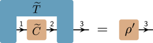
Figure 5: A quantum transformation T~\widetilde{T} which maps quantum channels C~\widetilde{C} into quantum states ρ\rho.

The next simplest transformation one could consider is a mapping from quantum channels to quantum states, i.e., transformations of the form T~[C12]=ρ3\widetilde{T}[C_{12}]=\rho_{3} (see Fig. 5).1111 11 Here, and in what follows, whenever there is no risk of confusion, we drop the semantic distinction between transformations and their respective Choi matrices. Such transformations are particular types of quantum combs [2, 5], and have been considered amongst others in the study of open quantum system dynamics with initial correlations under the name of \mathcal{M}-maps [28]. Keeping track of the involved spaces, for this case, we have to identify i12\mathcal{H}_{\textup{{{i}}}}\cong\mathcal{H}_{1}\otimes\mathcal{H}_{2} and o3\mathcal{H}_{\textup{{{o}}}}\cong\mathcal{H}_{3}. Since the resulting quantum states ρ3(3)\rho_{3}\in\mathcal{L}(\mathcal{H}_{3}) are unit trace, while tr[C12]=d1\tr[C_{12}]=d_{1}, we have γi=1\gamma_{\textup{{i}}}=1 and γo=d1\gamma_{\textup{{o}}}=d_{1}. Additionally, the role of P~i\widetilde{P}_{\textup{{{i}}}} is now played by the projector P~12(C)\widetilde{P}^{(C)}_{12} of Eq. (37b), while P~o\widetilde{P}_{\textup{{{o}}}} is again given by 𝟙~3\widetilde{\mathds{1}}_{3} (since there are no linear restrictions on quantum states). Given that all involved projectors are self-adjoint, unital and commute with the transposition, Thm. 2 applies. With this, using Eqs. (30a) and (30b), we obtain for the Choi state T123(123)T\in\mathcal{L}_{123}(\mathcal{H}_{1}\otimes\mathcal{H}_{2}\otimes\mathcal{H}_{3}) of the map T~\widetilde{T}:

(Quantum channel) (Quantum state)
C(12)C\in\mathcal{L}(\mathcal{H}_{1}\otimes\mathcal{H}_{2}) belongs to 𝒮i\mathcal{S}_{\textup{{i}}} iff ρ(3)\rho^{\prime}\in\mathcal{L}(\mathcal{H}_{3}) belongs to 𝒮o\mathcal{S}_{\textup{{o}}} iff
C0C\geq 0,     \mathbf{\longrightarrow} ρ0\rho^{\prime}\geq 0,
P~i[C]:=CC2+C12=C\widetilde{P}_{\textup{{i}}}[C]:=C-{}_{2}C+{}_{12}C=C, P~o[ρ]\widetilde{P}_{\textup{{o}}}[\rho^{\prime}] =𝟙~[ρ]=\widetilde{\mathbbm{1}}[\rho^{\prime}] =ρ=\rho^{\prime},
tr[C]=d1\tr[C]=d_{1}. tr[ρ]=1\tr[\rho^{\prime}]=1.
(Quantum ch annel to quantum state)
T\displaystyle T\geq\, 0,\displaystyle 0, (43a)
P~io[T]:=\displaystyle\widetilde{P}_{\textup{{i}}\textup{{o}}}[T]:=\, TT3+T23=T,\displaystyle T-{}_{3}T+{}_{23}T=T, (43b)
tr[T]=\displaystyle\tr[T]=\, d2.\displaystyle d_{2}\,. (43c)

The above coincides with T3=T23{}_{3}T={}_{23}T and tr[T]=d2\tr[T]=d_{2} which, in turn, are the causality/trace constraints of a one-slot comb with a final output line [5] (we discuss causality constraints in more detail below). Additionally, choosing 1\mathcal{H}_{1} to be trivial, i.e., 1\mathcal{H}_{1}\cong\mathbb{C}, we recover the characterisation of quantum channels. As before, demanding complete positivity from T~\widetilde{T} translates to the additional requirement T0T\geq 0. \blacksquare

Example 3 (Quantum channels to quantum channels (Quantum Superchannels)).

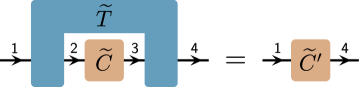
Let us now consider the question raised at the end of Sec. 2, namely the characterisation of transformations T~[C23]=C14\widetilde{T}[C_{23}]=C_{14}^{\prime} that map quantum channels C23(23)C_{23}\in\mathcal{L}(\mathcal{H}_{2}\otimes\mathcal{H}_{3}) onto quantum channels C14(14)C_{14}^{\prime}\in\mathcal{L}(\mathcal{H}_{1}\otimes\mathcal{H}_{4}) (see Fig. 6). In this case, we identify i23\mathcal{H}_{\textup{{{i}}}}\cong\mathcal{H}_{2}\otimes\mathcal{H}_{3} and o14\mathcal{H}_{\textup{{{o}}}}\cong\mathcal{H}_{1}\otimes\mathcal{H}_{4}. The projectors on the input and output space of T~\widetilde{T} are, respectively, given by the projectors P~23(C)\widetilde{P}^{(C)}_{23} and P~14(C)\widetilde{P}^{(C)}_{14} of Eq. (37b), which are self-adjoint, unital, and commute with the transposition, such that Thm. 2 applies. In addition, for channels, we have γi=tr[C23]=d2\gamma_{\textup{{i}}}=\tr[C_{23}]=d_{2} and γo=tr[C14]=d1\gamma_{\textup{{o}}}=\tr[C_{14}^{\prime}]=d_{1}. Thus, employing Eqs. (30a) and (30b), we obtain for the properties of T(1234)T\in\mathcal{L}(\mathcal{H}_{1}\otimes\mathcal{H}_{2}\otimes\mathcal{H}_{3}\otimes\mathcal{H}_{4}):

(Quantum channel) (Quantum channel)
C(23)C\in\mathcal{L}(\mathcal{H}_{2}\otimes\mathcal{H}_{3}) belongs to 𝒮i\mathcal{S}_{\textup{{i}}} iff C(14)C^{\prime}\in\mathcal{L}(\mathcal{H}_{1}\otimes\mathcal{H}_{4}) belongs to 𝒮o\mathcal{S}_{\textup{{o}}} iff
C0C\geq 0,     \mathbf{\longrightarrow} C0C^{\prime}\geq 0,
P~i[C]:=CC3+C23=C\widetilde{P}_{\textup{{i}}}[C]:=C-{}_{3}C+{}_{23}C=C, P~o[C]:=CC4+C14=C\widetilde{P}_{\textup{{o}}}[C^{\prime}]:=C^{\prime}-{}_{4}C^{\prime}+{}_{14}C^{\prime}=C^{\prime},
tr[C]=d2\tr[C]=d_{2}. tr[C]=d1\tr[C^{\prime}]=d_{1}.
(Quantum superchannel)
T\displaystyle T\geq 0,\displaystyle 0, (49a)
P~io[T]:=\displaystyle\widetilde{P}_{\textup{{i}}\textup{{o}}}[T]:= TT4+T34T234+T1234=T,\displaystyle T-{}_{4}T+{}_{34}T-{}_{234}T+{}_{1234}T=T, (49b)
tr[T]=\displaystyle\tr[T]= d1d3,\displaystyle d_{1}d_{3}\,, (49c)

It is easy to see that the above is, in addition to tr[T]=d1d3\tr[T]=d_{1}d_{3}, equivalent to T4=T34{}_{4}T={}_{34}T and T234=T1234{}_{234}T={}_{1234}T, which, in the ordering of spaces we have chosen, coincides with the causality/trace constraints of a quantum comb with one slot (corresponding to the spaces labelled by 22 and 33), and an initial input (labelled by 11) and final output (labelled by 44) [29]. This, in turn, reflects the well-known fact that there are no causally disordered superchannels [1]. Additionally, choosing 1\mathcal{H}_{1} to be trivial, we recover the conditions (49) on transformations of channels to states from above.

Finally, here, it is insightful to discuss in what way the properties of TT would change if the trace conditions on the elements of 𝒮i\mathcal{S}_{\textup{{i}}} and 𝒮o\mathcal{S}_{\textup{{o}}} were dropped. Then, the transformation T~:(23)(14){\widetilde{T}}^{\prime}:\mathcal{L}(\mathcal{H}_{2}\otimes\mathcal{H}_{3})\rightarrow\mathcal{L}(\mathcal{H}_{1}\otimes\mathcal{H}_{4}) would still have to satisfy (P~14(C)T~)[C23]=T~[C23](\widetilde{P}^{(C)}_{14}\circ\widetilde{T}^{\prime})[C_{23}]=\widetilde{T}^{\prime}[C_{23}] for all C23=P~23(C)[C23]C_{23}=\widetilde{P}^{(C)}_{23}[C_{23}], but it is not necessarily trace-rescaling. The corresponding characterisation for this case will be given in Thm. 4. Using Eq. (180) from Thm. 4 (see Sec. 8.3), one obtains

T=TP~23(C)[T]+(P~23(C)P~14(C))[T]=TT4+T14+T34T134T234+T1234,\displaystyle\begin{split}T^{\prime}&=T^{\prime}-\widetilde{P}^{(C)}_{23}[T^{\prime}]+(\widetilde{P}^{(C)}_{23}\otimes\widetilde{P}^{(C)}_{14})[T^{\prime}]\\ &=T^{\prime}-{}_{4}T^{\prime}+{}_{14}T^{\prime}+{}_{34}T^{\prime}-{}_{134}T^{\prime}-{}_{234}T^{\prime}+{}_{1234}T^{\prime},\end{split} (50)

with no additional restriction on the trace of TT^{\prime}. Even setting aside the absence of an additional trace constraint on TT^{\prime}, the above Equation is significantly different from Eq. (49b), underlining the importance of the affine constraints on 𝒮i\mathcal{S}_{\textup{{i}}} and 𝒮o\mathcal{S}_{\textup{{o}}} for the properties of the transformations between them. \blacksquare

Figure 6: Superchannels. A superchannel T~\widetilde{T} maps a CPTP map C~\widetilde{C} onto a CPTP map C~\widetilde{C}^{\prime}.
Example 4 (Quantum superchannels to quantum channels (Two-slot combs)).

Let us now consider the question of transforming superchannels into channels (see Fig. 7), such mathematical objects are known in the literature as two-slot quantum combs [2, 1, 5], two-round quantum strategies [3], and two-slot sequential superchannels [30]. In this case, we identify i2345\mathcal{H}_{\textup{{{i}}}}\cong\mathcal{H}_{2}\otimes\mathcal{H}_{3}\otimes\mathcal{H}_{4}\otimes\mathcal{H}_{5} and o16\mathcal{H}_{\textup{{{o}}}}\cong\mathcal{H}_{1}\otimes\mathcal{H}_{6}. Thus, employing the projectors from the previous examples, we obtain for the properties of T(123456)T\in\mathcal{L}(\mathcal{H}_{1}\otimes\mathcal{H}_{2}\otimes\mathcal{H}_{3}\otimes\mathcal{H}_{4}\otimes\mathcal{H}_{5}\otimes\mathcal{H}_{6}):

(Quantum superchannel) (Quantum channel)
C(2345)C\in\mathcal{L}(\mathcal{H}_{2}\otimes\mathcal{H}_{3}\otimes\mathcal{H}_{4}\otimes\mathcal{H}_{5}) C(16)C^{\prime}\in\mathcal{L}(\mathcal{H}_{1}\otimes\mathcal{H}_{6})
belongs to 𝒮i\mathcal{S}_{\textup{{i}}} iff \mathbf{\longrightarrow} belongs to 𝒮o\mathcal{S}_{\textup{{o}}} iff
C0C\geq 0, C0C^{\prime}\geq 0,
P~i[C]:=CC5+C45C345+C2345=C\widetilde{P}_{\textup{{i}}}[C]:=C-{}_{5}C+{}_{45}C-{}_{345}C+{}_{2345}C=C, P~o[C]:=CC6+C16=C\widetilde{P}_{\textup{{o}}}[C^{\prime}]:=C^{\prime}-{}_{6}C^{\prime}+{}_{16}C^{\prime}=C^{\prime},
tr[C]=d2d4\tr[C]=d_{2}d_{4}. tr[C]=d1\tr[C^{\prime}]=d_{1}.
(Quantum two-slot comb)
T\displaystyle T\geq 0,\displaystyle 0, (57a)
P~io[T]:=\displaystyle\widetilde{P}_{\textup{{i}}\textup{{o}}}[T]:= TT6+T56T456+T3456T23456+T123456=T,\displaystyle T-{}_{6}T+{}_{56}T-{}_{456}T+{}_{3456}T-{}_{23456}T+{}_{123456}T=T, (57b)
tr[T]=\displaystyle\tr[T]= d1d3d5.\displaystyle d_{1}d_{3}d_{5}. (57c)
Refer to caption
Figure 7: Two-slot combs. A two-slot comb T~\widetilde{T} maps a superchannel C~\widetilde{C} onto a CPTP map C~\widetilde{C}^{\prime}.

Two-slots quantum combs are known to be causally ordered since they may always be decomposed as a quantum circuit [2, 1, 5, 3], that is, as an ordered sequence of quantum channels, as illustrated in Fig. 8. As discussed in the next example, this causally ordered property also holds for any (k+1)(k+1)-slot quantum comb, which is a quantum transformation from a kk-slot comb into a quantum channel [5]. \blacksquare

Refer to caption
Figure 8: Two-slot combs. A two-slot comb T~\widetilde{T} can always be decomposed as a sequence of CPTP maps {G~1,G~2,G~3}\{\widetilde{G}_{1},\widetilde{G}_{2},\widetilde{G}_{3}\}.
Example 5 (Quantum (k1)(k-1)-slot combs to quantum channels (kk-slot combs)).

Let us now consider the question of transforming (k1)(k-1)-slot combs into channels (see Fig. 9), such mathematical objects are known in the literature as kk-slot quantum combs [2, 1, 5], kk-round quantum strategies [3], and kk-slot sequential superchannels [30].

Definition 3.

A 00-slot quantum comb is a quantum channel. For an arbitrary kk\in\mathbb{N}, a kk-slot quantum comb is recursively defined as a quantum transformation which maps (k1)(k-1)-quantum combs into quantum channels.

In this case, we identify i232k+1\mathcal{H}_{\textup{{{i}}}}\cong\mathcal{H}_{2}\otimes\mathcal{H}_{3}\otimes\ldots\mathcal{H}_{2{k}+1} and o12k+2\mathcal{H}_{\textup{{{o}}}}\cong\mathcal{H}_{1}\otimes\mathcal{H}_{{2k+2}}. Thus, employing the results from previous examples, we obtain for the properties of T(122k+2)T\in\mathcal{L}(\mathcal{H}_{1}\otimes\mathcal{H}_{2}\ldots\otimes\mathcal{H}_{2k+2}):

((k1k-1)-slot comb) (Quantum channel)
C(232k+1)C\in\mathcal{L}(\mathcal{H}_{2}\otimes\mathcal{H}_{3}\otimes\ldots\otimes\mathcal{H}_{2k+1}) C(12k+2)C^{\prime}\in\mathcal{L}(\mathcal{H}_{1}\otimes\mathcal{H}_{2k+2})
belongs to 𝒮i\mathcal{S}_{\textup{{i}}} iff \mathbf{\longrightarrow} belongs to 𝒮o\mathcal{S}_{\textup{{o}}} iff
C0C\geq 0, C0C^{\prime}\geq 0,
P~i[C]:=CC(2k+1)+C(2k)(2k+1)\widetilde{P}_{\textup{{i}}}[C]:=C-{}_{(2k+1)}C+{}_{(2k)(2k+1)}C-\ldots P~o[C]:=CC(2k+2)\widetilde{P}_{\textup{{o}}}[C^{\prime}]:=C^{\prime}-{}_{(2k+2)}C^{\prime}
asdfffffffC3(2k+1)+C2(2k+1)=C,-{}_{3\ldots(2k+1)}C+{}_{2\ldots(2k+1)}C=C, asdfffffffffffffff+C1(2k+2)=C+{}_{1(2k+2)}C^{\prime}=C^{\prime},
tr[C]=d2d4d2k\tr[C]=d_{2}d_{4}\ldots d_{2k}. tr[C]=d1\tr[C^{\prime}]=d_{1}.
(Quantum 𝐤\mathbf{k}-slot comb)
T\displaystyle T\geq 0\displaystyle 0 (65a)
P~io[T]:=\displaystyle\widetilde{P}_{\textup{{i}}\textup{{o}}}[T]:= TT(2k+2)+T(2k+1)(2k+2)T(2k)(2k+1)(2k+2)+\displaystyle T-{}_{(2k+2)}T+{}_{(2k+1)(2k+2)}T-{}_{(2k)(2k+1)(2k+2)}T+\phantom{f}
T23(2k+2)+T12(2k+2)=T,\displaystyle\ldots-{}_{23\ldots(2k+2)}T+{}_{12\ldots(2k+2)}T=T,
tr[T]=\displaystyle\tr[T]= d1d3d5d(2k+1),\displaystyle d_{1}d_{3}d_{5}\ldots d_{(2k+1)}\,,
Refer to caption
Figure 9: kk-slot combs. A kk-slot comb T~\widetilde{T} maps a (k1)(k-1)-slot comb C~\widetilde{C} onto a CPTP map C~\widetilde{C}^{\prime}.

All kk-slots quantum combs may be decomposed as a quantum circuit [2, 1, 5, 3], that is, as an ordered sequence of quantum channels, as illustrated in Fig. 8. \blacksquare

Refer to caption
Figure 10: kk-slot combs. A kk-slot comb can always be decomposed as an ordered sequence of quantum channels.

4.1 Transformations without a fixed causal order

All quantum transformations addressed in previous could be decomposed in terms of an ordered quantum circuit. For this reason, they are referred to as objects with a fixed causal order. As proven in Ref. [5], a quantum transformation admits a decomposition as a fixed ordered quantum circuit if it is a quantum kk-slot comb. This motivates the definition of transformations with a fixed order.

Definition 4.

A quantum transformation T~\widetilde{T} has a fixed causal order if it can be written as a kk-slot comb for some well-suited dimensions, where we may also set some of the dimensions to be one.

While the concept of fixed causal order is well-established, there are non-equivalent definitions for which transformations have a definite causal order. One of the first articles to define definite causal order considered the scenario of process matrices which transform a pair of independent channels to unit probability [8] (this case is discussed in the next example). There, a quantum transformation does not have a definite causal order if it cannot be written as a convex combination of quantum transformations with fixed order, a definition which is well-established for this ‘bipartite’ process matrix scenario. When more general quantum transformations are considered, e.g., transformations of a pair of quantum channels into a channel, different arguments led to alternative notions of indefinite causal order [31, 32]. Additionally, when more than two parties are involved, the concept of classical dynamical control of causal order plays a non-trivial role [33]. Here, we will stay clear of these (important) subtleties in the definition of causal definiteness, and only examine if the obtained transformations can lie outside the set of fixed causal order processes, i.e., outside the set of quantum combs.

Example 6 (Non-signalling channels to unit probability (Process Matrix)).

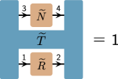
As a pertinent example, let us consider the well-studied case of (bipartite) process matrices [8, 15], i.e., the set of transformations T~\widetilde{T} that map pairs of CPTP maps to unit probability (this, in turn, implies that they constitute the dual affine set of the set of (bipartite) non-signalling CPTP maps, see Sec. 7). Specifically, let R12R_{12} and N34N_{34} be the Choi states of CPTP maps R~:(1)(2)\widetilde{R}:\mathcal{L}(\mathcal{H}_{1})\rightarrow\mathcal{L}(\mathcal{H}_{2}) and N~:(3)(4)\widetilde{N}:\mathcal{L}(\mathcal{H}_{3})\rightarrow\mathcal{L}(\mathcal{H}_{4}). Then, the set of process matrices is given by all linear maps T~:(1234)\widetilde{T}:\mathcal{L}(\mathcal{H}_{1}\otimes\mathcal{H}_{2}\otimes\mathcal{H}_{3}\otimes\mathcal{H}_{4})\rightarrow\mathbbm{C} such that T~[R12N34]=1\widetilde{T}[R_{12}\otimes N_{34}]=1 for all CPTP maps R12,N34R_{12},N_{34}. In this case, the input space is given by i=1234\mathcal{H}_{\textup{{{i}}}}=\mathcal{H}_{1}\otimes\mathcal{H}_{2}\otimes\mathcal{H}_{3}\otimes\mathcal{H}_{4}, while o=\mathcal{H}_{\textup{{{o}}}}=\mathbbm{C}. The corresponding projectors simply follow from the previous examples as P~i=P~12(C)P~34(C)\widetilde{P}_{\textup{{{i}}}}=\widetilde{P}^{(C)}_{12}\otimes\widetilde{P}^{(C)}_{34} and P~o=𝟙~\widetilde{P}_{\textup{{{o}}}}=\widetilde{\mathds{1}} (these are, again, self-adjoint and unital projectors that commute with the transpose, such that Thm. 2 can be applied). More explicitly, we have

P~i[M]=\displaystyle\widetilde{P}_{\textup{{i}}}[M]= P~12(C)P~34(C)[M]\displaystyle\widetilde{P}^{(C)}_{12}\otimes\widetilde{P}^{(C)}_{34}[M] (66)
=\displaystyle= P~12(C)[MM4+M34]\displaystyle\widetilde{P}^{(C)}_{12}[M-{}_{4}M+{}_{34}M] (67)
=\displaystyle= (MM4+M34)(MM4+M34)2+(MM4+M34)12\displaystyle(M-{}_{4}M+{}_{34}M)-{}_{2}(M-{}_{4}M+{}_{34}M)+{}_{12}(M-{}_{4}M+{}_{34}M) (68)
=\displaystyle= MM4+M34M2+M24M234+M12M124+M1234.\displaystyle M-{}_{4}M+{}_{34}M-{}_{2}M+{}_{24}M-{}_{234}M+{}_{12}M-{}_{124}M+{}_{1234}M. (69)

With this, we can employ Eqs. (30a) and (30b) to obtain the properties of process matrices T(1234)T\in\mathcal{L}(\mathcal{H}_{1}\otimes\mathcal{H}_{2}\otimes\mathcal{H}_{3}\otimes\mathcal{H}_{4}) that send pairs of CPTP maps to unit probability:

   
(Non-signalling channel) (Complex number)
M(1234)M\in\mathcal{L}(\mathcal{H}_{1}\otimes\mathcal{H}_{2}\otimes\mathcal{H}_{3}\otimes\mathcal{H}_{4}) belongs to 𝒮i\mathcal{S}_{\textup{{i}}} iff c()c\in\mathcal{L}(\mathbb{C}) belongs to 𝒮o\mathcal{S}_{\textup{{o}}} iff
M0M\geq 0, c0c\geq 0,
P~i[M]:=MM2M4+M24+M34\widetilde{P}_{\textup{{i}}}[M]:=M-{}_{2}M-{}_{4}M+{}_{24}M+{}_{34}M- \mathbf{\longrightarrow} P~o[c]:=c\widetilde{P}_{\textup{{o}}}[c]:=c,
M234+M12M124+M1234=M\phantom{\widetilde{P}_{\textup{{i}}}[M]}{}_{234}M+{}_{12}M-{}_{124}M+{}_{1234}M=M, tr[c]=1\tr[c]=1.
tr[M]=d1d3\tr[M]=d_{1}d_{3}.
(Process matrix)
T\displaystyle T\geq\, 0,\displaystyle 0, (76a)
P~io[T]:=\displaystyle\widetilde{P}_{\textup{{i}}\textup{{o}}}[T]:=\, T2+T4T24T34+T234T12+T124=T,\displaystyle{}_{2}T+{}_{4}T-{}_{24}T-{}_{34}T+{}_{234}T-{}_{12}T+{}_{124}T=T, (76b)
tr[T]=\displaystyle\tr[T]=\, d2d4.\displaystyle d_{2}d_{4}\,. (76c)

The above properties of TT exactly coincide with the characterisation of process matrices given in Ref. [15]. \blacksquare

(a)
(b)
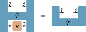
Figure 11: (a) Process Matrix. As a mapping from two independent channels R~\widetilde{R} and N~\widetilde{N} to the number 11 (b) Process Matrix. As a mapping from a channel R~\widetilde{R} to a one-slot superchannel Q~\widetilde{Q}^{\prime} without past and future.

In particular this latter result is of interest, since the set of process matrices can be considered the dual affine set of the set of all tensor products of CPTP maps, where the dual affine of a set are all operators that map the elements of the set to 11.1212 12 More generally, any process matrix TT will map any matrix of the form iλiM(i)N(i)\sum_{i}\lambda_{i}M^{(i)}\otimes N^{(i)}, where iλi=1\sum_{i}\lambda_{i}=1, and M(i),N(i)M^{(i)},N^{(i)} CPTP to 11. Since the set of all valid CPTP maps that can be decomposed in this way is the set of non-signalling maps [34, 35], process matrices form exactly the dual set of non-signalling maps. We will further investigate this connection in Sec. 7. Such dual affine sets play an important role in quantum mechanics (and more generally, linear algebra), and evidently, the projectors we introduced can be used to characterise them comprehensively. Below, we will analyse the characterisation of dual sets (affine or not) in more detail. Before doing so, we provide an alternative characterisation of process matrices.

Example 7 (Quantum channels to superchannels without initial input and final output (Process matrices revisited)).

As a penultimate example, let us consider process matrices from a different perspective. Interestingly, they can be characterised in an alternative (yet equivalent) way, namely as mappings that map quantum channels (say, R~:(1)(2)\widetilde{R}:\mathcal{L}(\mathcal{H}_{1})\rightarrow\mathcal{L}(\mathcal{H}_{2})) to one-slot combs with no initial input and final output, i.e., superchannels with trivial input and output space (see Fig. 11(b)). Concretely, this requirement reads T~[R]=Q~\widetilde{T}[R]={\widetilde{Q}}^{\prime}, where Q~{\widetilde{Q}}^{\prime} is a one-slot comb whenever R~\widetilde{R} is a CPTP map. Since such one-slot combs are special cases of superchannels, they are characterised by the projector of Eq. (49b) and they have a fixed causal order, that is, they can be represented by a causally ordered quantum circuit. This latter fact, in turn, chimes nicely with the intuitive definition of process matrices as mappings that obey local but not necessarily global causality [8]; considering the slot corresponding to 1\mathcal{H}_{1} and 2\mathcal{H}_{2} as Alice’s laboratory, independent of what deterministic operation (i.e., CPTP map) she performs locally, Bob (i.e., the slot corresponding to 3\mathcal{H}_{3} and 4\mathcal{H}_{4}) will always encounter a causally ordered scenario (given by the one-slot comb Q~\widetilde{Q}^{\prime}). Naturally, one would obtain the same definition of process matrices with the roles of Alice and Bob reversed.

Let us now show that this alternative definition of process matrices indeed leads to the same characterisation as the one provided in the previous Example. First, since R12(12)R_{12}\in\mathcal{L}(\mathcal{H}_{1}\otimes\mathcal{H}_{2}) and Q34(34)Q^{\prime}_{34}\in\mathcal{L}(\mathcal{H}_{3}\otimes\mathcal{H}_{4}), we identify i(12)\mathcal{H}_{\textup{{{i}}}}\cong\mathcal{L}(\mathcal{H}_{1}\otimes\mathcal{H}_{2}) and o(34)\mathcal{H}_{\textup{{{o}}}}\cong\mathcal{L}(\mathcal{H}_{3}\otimes\mathcal{H}_{4}). The projector P~i\widetilde{P}_{\textup{{{i}}}} is given by the projector P~12(C)\widetilde{P}^{(C)}_{12} on the space of channels, while P~o\widetilde{P}_{\textup{{{o}}}} follows directly from the projector onto the set of superchannels provided in Eq. (49b) by setting 14\mathcal{H}_{1}\cong\mathcal{H}_{4}\cong\mathbbm{C}, such that P~o[T]=T4\widetilde{P}_{\textup{{{o}}}}[T]={}_{4}T. Additionally, we have that γi=tr[R]=d2\gamma_{\textup{{i}}}=\tr[R]=d_{2}, while γo=tr[Q]=d3\gamma_{\textup{{o}}}=\tr[Q^{\prime}]=d_{3} (see Eq. (49)). Since all involved projectors are self-adjoint, unital, and commute with the transposition, Thm. 2 applies, and we obtain the characterisation of T as

(Quantum channel) (Superchannel without past and future)
R(12)R\in\mathcal{L}(\mathcal{H}_{1}\otimes\mathcal{H}_{2}) belongs to 𝒮i\mathcal{S}_{\textup{{i}}} iff Q(34)Q^{\prime}\in\mathcal{L}(\mathcal{H}_{3}\otimes\mathcal{H}_{4}) belongs to 𝒮o\mathcal{S}_{\textup{{o}}} iff
R0R\geq 0, \mathbf{\longrightarrow} Q0Q^{\prime}\geq 0,
P~i[R]:=RR2+R12=R\widetilde{P}_{\textup{{i}}}[R]:=R-{}_{2}R+{}_{12}R=R, P~o[Q]:=Q4=Q\widetilde{P}_{\textup{{o}}}[Q^{\prime}]:={}_{4}Q^{\prime}=Q^{\prime},
tr[R]=d1\tr[R]=d_{1}. tr[Q]=d3\tr[Q^{\prime}]=d_{3}.
(Process matrix revisited)
T\displaystyle T\geq\, 0,\displaystyle 0, (82a)
P~io[T]:=\displaystyle\widetilde{P}_{\textup{{i}}\textup{{o}}}[T]:=\, T2+T4T24T34+T234T12+T124=T,\displaystyle{}_{2}T+{}_{4}T-{}_{24}T-{}_{34}T+{}_{234}T-{}_{12}T+{}_{124}T=T, (82b)
tr[T]=\displaystyle\tr[T]=\, d2d4,\displaystyle d_{2}d_{4}\,, (82c)

which coincides exactly with the characterisation of process matrices given in Eq. (76). Besides yielding an equivalent characterisation of process matrices, the above derivation also sheds an interesting light on the emergence of causal indefiniteness; graphically, a mapping from CPTP maps to one-slot combs is very similar to a mapping from CPTP maps to CPTP maps (i.e., superchannels), with the only difference that the incoming and outgoing wires of the former case are inverted with respect to the latter (to see this, compare Figs. 6 and 11(b)). This graphical similarity notwithstanding, all one-slot superchannels have a fixed causal order, while process matrices do not always have an ordered quantum circuit decomposition (since the projector in Eq. (82b) is not onto the space of 22-slot combs). In particular, process matrices can be causally non-separable, that is, they cannot be written as a convex combination of ordered quantum circuits, or even as a quantum circuit with classical dynamical order [33], and may even violate causal inequalities [8, 36].

Finally, let us remark that the equivalence between the two characterisations of process matrices ceases to hold if the trace-rescaling property is dropped. In this case, the requirement that process matrices map non-signalling maps to \mathbbm{C}(i.e., the case considered in the previous Example) yields no restrictions on the corresponding map TT^{\prime}, i.e., P~io=𝟙~io\widetilde{P}_{\textup{{{i}}{{o}}}}=\widetilde{\mathds{1}}_{\textup{{{i}}{{o}}}} (as can be seen by direct insertion into Eq. (180) in Sec. 8.3). On the other hand, dropping the trace-rescaling conditions on maps that map CPTP maps to the space spanned by one-slot combs (i.e., the ones considered in this Example), we obtain, using Thm. 4:

T=T2+T4T24T12+T124,\displaystyle T^{\prime}={}_{2}T^{\prime}+{}_{4}T^{\prime}-{}_{24}T^{\prime}-{}_{12}T^{\prime}+{}_{124}T^{\prime}, (83)

which is a non-trivial constraint on the map TT^{\prime}. \blacksquare

Example 8 (Superchannels to superchannels).

We now discuss an a priori more involved case that features less prominently in the literature: mappings from superchannels to superchannels (see Fig. 12). Above, we already derived the projector onto the space of superchannels as well as their trace (see Eqs. (49)).

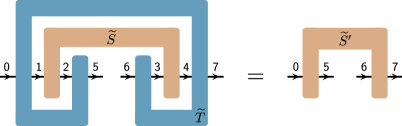
Figure 12: Superchannel to superchannel. The higher-order quantum map T~\widetilde{T} (with Choi matrix T(01256347)T\in\mathcal{L}(\mathcal{H}_{0}\otimes\mathcal{H}_{1}\otimes\mathcal{H}_{2}\otimes\mathcal{H}_{5}\otimes\mathcal{H}_{6}\otimes\mathcal{H}_{3}\otimes\mathcal{H}_{4}\otimes\mathcal{H}_{7}) maps superchannels S~\widetilde{S} (with Choi state S(1234)S\in\mathcal{L}(\mathcal{H}_{1}\otimes\mathcal{H}_{2}\otimes\mathcal{H}_{3}\otimes\mathcal{H}_{4})) onto superchannels S~{\widetilde{S}}^{\prime} (with Choi state S(0567𝐶𝐿𝑂𝑆𝐸S^{\prime}\in\mathcal{L}(\mathcal{H}_{0}\otimes\mathcal{H}_{5}\otimes\mathcal{H}_{6}\otimes\mathcal{H}_{7})).

Here, proper bookkeeping of the involved spaces becomes slightly involved, but the respective properties of mappings from superchannels to superchannels can be readily deduced, using Thm. 2. Specifically, following the labelling convention of Fig. 12, we set i:=1234\mathcal{H}_{\textup{{i}}}:=\mathcal{H}_{1}\otimes\mathcal{H}_{2}\otimes\mathcal{H}_{3}\otimes\mathcal{H}_{4} and o:=0567\mathcal{H}_{\textup{{o}}}:=\mathcal{H}_{0}\otimes\mathcal{H}_{5}\otimes\mathcal{H}_{6}\otimes\mathcal{H}_{7}. Consequently, for the Choi matrices SS (SS^{\prime}) of the input (output) superchannels we have S(i)S\in\mathcal{L}(\mathcal{H}_{\textup{{i}}}) (S(o)S^{\prime}\in\mathcal{L}(\mathcal{H}_{\textup{{o}}}) ), while the Choi matrix TT of the transformation between them acts on io\mathcal{H}_{\textup{{i}}}\otimes\mathcal{H}_{\textup{{o}}}. Now, using Thm. 2, we obtain

(Superchannel) (Superchannel)
S(1234)𝒮iS\in\mathcal{L}(\mathcal{H}_{1}\otimes\mathcal{H}_{2}\otimes\mathcal{H}_{3}\otimes\mathcal{H}_{4})\in\mathcal{S}_{\textup{{i}}} iff S(0567)𝒮oS^{\prime}\in\mathcal{L}(\mathcal{H}_{0}\otimes\mathcal{H}_{5}\otimes\mathcal{H}_{6}\otimes\mathcal{H}_{7})\in\mathcal{S}_{\textup{{o}}} iff
S0S\geq 0, \mathbf{\longrightarrow} S0S^{\prime}\geq 0,
P~i[S]:=SS4+S34\widetilde{P}_{\textup{{i}}}[S]:=S-{}_{4}S+{}_{34}S, P~o[S]:=SS7+S67\widetilde{P}_{\textup{{o}}}[S^{\prime}]:=S^{\prime}-{}_{7}S^{\prime}+{}_{67}S^{\prime},
P~i[S]:====\widetilde{P}_{\textup{{i}}}[S]:==== S234+S1234=S-{}_{234}S+{}_{1234}S=S, P~i[S]:====\widetilde{P}_{\textup{{i}}}[S]:====S567+S0567=S-{}_{567}S^{\prime}+{}_{0567}S^{\prime}=S^{\prime},
tr[S]=d1d3\tr[S]=d_{1}d_{3}. tr[S]=d0d6\tr[S^{\prime}]=d_{0}d_{6}.
(Mapping bet ween superchannels)
T\displaystyle T\geq 0,\displaystyle\ 0, (90a)
P~io[T]:=\displaystyle\widetilde{P}_{\textup{{i}}\textup{{o}}}[T]:= TT7+T47+T67T347T467T567+T2347\displaystyle\ T-{}_{7}T+{}_{47}T+{}_{67}T-{}_{347}T-{}_{467}T-{}_{567}T+{}_{2347}T
+T3467+T4567T12347T23467T34567+T123467,\displaystyle+{}_{3467}T+{}_{4567}T-{}_{12347}T-{}_{23467}T-{}_{34567}T+{}_{123467}T,
+T234567T1234567+T01234567=T.\displaystyle+{}_{234567}T-{}_{1234567}T+{}_{01234567}T=T. (90b)
tr[T]=\displaystyle\tr[T]= d0d6d2d4.\displaystyle d_{0}d_{6}d_{2}d_{4}\,. (90c)

While not a priori particularly insightful (albeit indispensable when numerically optimising over transformations of superchannels) in its own right, Eq. (90b) allows one to directly deduce that transformations from superchannels to superchannels do not necessarily display a fixed causal order, i.e., they are not limited to quantum combs and cannot necessarily be implemented by means of a quantum circuit. In particular, counting input and output spaces, if TT corresponded to a supermap with a fixed causal order, it would have to satisfy the properties of a 33-slot comb (see Fig. 12). For example, for the space 7\mathcal{H}_{7} to be the final output space of such a 33-slot comb, TT would have to satisfy T7=Tx7{}_{7}T={}_{\texttt{x}7}T, where x{0,2,4,6}\texttt{x}\in\{0,2,4,6\}. From Eq. (90b), we directly see that this is not the case for any x, and, for instance, we have T7T47=T67T467T567+T45670{}_{7}T-{}_{47}T={}_{67}T-{}_{467}T-{}_{567}T+{}_{4567}T\neq 0 and analogously for x=0,2,6\texttt{x}=0,2,6. In a similar vein, this can be checked for the other potential final output spaces {1,5,3}\{1,5,3\}, with the same result. Consequently, there exists valid general maps from superchannels to superchannels which do not have a fixed causal order. \blacksquare

Example 9 (Unital channels to unital channels).

As a last example, we will now consider transformations mapping unital channels to unital channels. A linear map C~:(i)(o)\widetilde{C}:\mathcal{L}(\mathcal{H}_{\textup{{i}}})\to\mathcal{L}(\mathcal{H}_{\textup{{o}}}) is unital if it preserves the identity operator, i.e., C~(𝟙i)=𝟙o\widetilde{C}(\mathds{1}_{\textup{{i}}})=\mathds{1}_{\textup{{o}}}, in Choi picture if C(io)C\in\mathcal{L}(\mathcal{H}_{\textup{{i}}}\otimes\mathcal{H}_{\textup{{o}}}) is the Choi operator of the channel C~\widetilde{C}, C~\widetilde{C} is unital if and only if tri(C)=𝟙o\tr_{\textup{{i}}}(C)=\mathds{1}_{\textup{{o}}}. Quantum channels which are unital are also referred to it as bistochastic channels. Transformations between them were first analysed in Ref. [37], where the authors introduced the “quantum time flip”, object which was explored in an experimental context in Ref. [38, 39].

Here, it is important to notice that, since unital maps do not span the set of all CPTP maps, the most general quantum transformation mapping unital channels into unital channels may transform quantum channels into objects which are not quantum channels. For concreteness, we now illustrate this fact with the example discussed in Ref. [37]. Let i:=12\mathcal{H}_{\textup{{i}}}:=\mathcal{H}_{1}\otimes\mathcal{H}_{2} and o:=03\mathcal{H}_{\textup{{o}}}:=\mathcal{H}_{0}\otimes\mathcal{H}_{3}, and T~:(i)(o)\widetilde{T}:\mathcal{L}(\mathcal{H}_{\textup{{i}}})\to\mathcal{L}(\mathcal{H}_{\textup{{o}}}) be defined as T~(C)=FCF\widetilde{T}(C)=FCF^{\dagger}, where F:12F:\mathcal{H}_{1}\to\mathcal{H}_{2} is the flip operator (also known as swap operator) defined as F:=ij|ijji|F:=\sum_{ij}|ij\rangle\hskip-1.13809pt\langle ji|. We notice that, if we apply T~\widetilde{T} on unital channels B(i)B\in\mathcal{L}(\mathcal{H}_{\textup{{i}}}), the output T~(B)\widetilde{T}(B) is a quantum channel. However, if we apply the map T~\widetilde{T} to non-unital channels, such as a trace and replace one C=𝟙1|00|C=\mathds{1}_{1}\otimes|0\rangle\hskip-1.13809pt\langle 0|, we have that T~(𝟙1|00|2)=|00|1𝟙3\widetilde{T}(\mathds{1}_{1}\otimes|0\rangle\hskip-1.13809pt\langle 0|_{2})=|0\rangle\hskip-1.13809pt\langle 0|_{1}\otimes\mathds{1}_{3}, which is not a quantum channel, because tr3(|00|0𝟙3)𝟙0\tr_{3}(|0\rangle\hskip-1.13809pt\langle 0|_{0}\otimes\mathds{1}_{3})\neq\mathds{1}_{0}. Hence, such class of transformations go beyond the process matrix formalism [8] but can still be characterised via Thm. 2, illustrating the generality of our methods.

Similarly to the other cases, we now invoke Thm. 2, to obtain

(Unital channel) (Unital channel)
C(12)𝒮iC\in\mathcal{L}(\mathcal{H}_{1}\otimes\mathcal{H}_{2})\in\mathcal{S}_{\textup{{i}}} iff C(03)𝒮oC^{\prime}\in\mathcal{L}(\mathcal{H}_{0}\otimes\mathcal{H}_{3})\in\mathcal{S}_{\textup{{o}}} iff
C0C\geq 0, \mathbf{\longrightarrow} C0C^{\prime}\geq 0,
P~i[C]:=CC1C2+2C12=C\widetilde{P}_{\textup{{i}}}[C]:=C-{}_{1}C-{}_{2}C+2{}_{12}C=C, P~o[S]:=CC0C3+2C03=C\widetilde{P}_{\textup{{o}}}[S^{\prime}]:=C^{\prime}-{}_{0}C^{\prime}-{}_{3}C^{\prime}+2{}_{03}C^{\prime}=C^{\prime},
tr[S]=d1\tr[S]=d_{1}. tr[S]=d0\tr[S^{\prime}]=d_{0}.
(Mapping b etween unital channels)
T\displaystyle T\geq 0,\displaystyle\ 0, (96a)
P~io[T]:=\displaystyle\widetilde{P}_{\textup{{i}}\textup{{o}}}[T]:= T0T+01T+02T2012T3T+13T+23T2123T\displaystyle\ T-_{0}T+_{01}T+_{02}T-2_{012}T-_{3}T+_{13}T+_{23}T-2_{123}T
+03T013T023T+30123T=T\displaystyle+_{03}T-_{013}T-_{023}T+3_{0123}T=T (96b)
tr[T]=\displaystyle\tr[T]= d0d3.\displaystyle d_{0}d_{3}\,. (96c)

When compared to the appendix “Characterisation of the operations on bistochastic channels” of Ref. [37], the equations above provide an alternative (but equivalent) characterisation of transformations between unital channels \blacksquare

5 ‘Completeness’ of Quantum properties

5.1 Completely admissible transformations

Up to this point, we have discussed the properties of transformations T~io\widetilde{T}_{\textup{{i}}\textup{{o}}} whenever they act non-trivially on the full input space (i)\mathcal{L}(\mathcal{H}_{\textup{{i}}}). However, just like in the case of positivity, one may wonder if a transformation is also admissible (in a sense to be defined below) when only acting non-trivially on a part of an input object Wia(ia)W_{\textup{{i}}\textup{{a}}}\in\mathcal{L}(\mathcal{H}_{\textup{{i}}}\otimes\mathcal{H}_{\textup{{a}}}). To give a simple concrete example, a trace-preserving map T~io\widetilde{T}_{\textup{{i}}\textup{{o}}} is also trace preserving when only acting non-trivially on a part of a quantum state ρia(ia)\rho_{\textup{{i}}\textup{{a}}}\in\mathcal{L}(\mathcal{H}_{\textup{{i}}}\otimes\mathcal{H}_{\textup{{a}}}), i.e., tr[T~io𝟙~a[ρia]]=tr[ρia]\tr[\widetilde{T}_{\textup{{i}}\textup{{o}}}\otimes\widetilde{\mathds{1}}_{\textup{{a}}}[\rho_{\textup{{i}}\textup{{a}}}]]=\tr[\rho_{\textup{{i}}\textup{{a}}}] for all auxiliary spaces (a)\mathcal{L}(\mathcal{H}_{\textup{{a}}}). A priori, though, it is unclear if, and even in what sense, this ‘completeness’ holds for more involved cases, like the ones discussed in the previous section. To tackle this question, we first require the notion of an extension of a projector:

Definition 5 (Extension of a projector).

For a given projector P~x\widetilde{P}_{\textup{{x}}} on (x)\mathcal{L}(\mathcal{H}_{\textup{{x}}}), we call a family of projectors {P~xa}a\{\widetilde{P}_{\textup{{x}}\textup{{a}}}\}_{\textup{{a}}} on the respective spaces (xa)\mathcal{L}(\mathcal{H}_{\textup{{x}}}\otimes\mathcal{H}_{\textup{{a}}}) an extension of P~x\widetilde{P}_{\textup{{x}}} if it satisfies P~xaP~x\widetilde{P}_{\textup{{x}}\textup{{a}}}\cong\widetilde{P}_{\textup{{x}}} when a\mathcal{H}_{\textup{{a}}}\cong\mathbbm{C}. Additionally, whenever P~x\widetilde{P}_{\textup{{x}}} is self-adjoint (unital, commuting with the transposition), all projectors of the extension are assumed to be self-adjoint (unital, commuting with the transposition)

Whenever there is no risk of confusion, we also call the individual projectors P~xa\widetilde{P}_{\textup{{x}}\textup{{a}}} an extension of P~x\widetilde{P}_{\textup{{x}}}, with the understanding that they are an element of a whole set of projection operators. A priori, the above definition occurs somewhat void of meaning, since it does not really restrict the set of extensions {P~xa}a\{\widetilde{P}_{\textup{{x}}\textup{{a}}}\}_{\textup{{a}}}. We emphasise that this is by design, since we aim to remain agnostic with respect to how one chooses a particular extension in a concrete physical scenario; choosing a more restrictive definition of an extension1313 13 A seemingly obvious additional restriction would be of the form traP~xaP~x\tr_{\textup{{a}}}\circ\widetilde{P}_{\textup{{x}}\textup{{a}}}\propto\widetilde{P}_{\textup{{x}}}. While this is the case in all the examples we provide, this assumes a particular relationship between all the spaces defined by {P~xa}a\{\widetilde{P}_{\textup{{x}}\textup{{a}}}\}_{\textup{{a}}}, which we do not fundamentally require for our proofs/constructions. might exclude many cases of interest. Since this level of generality does not pose any additional technical issues, we thus postpone more explicit definitions of the extensions to the examples below (see Exs. 10 and 11).

For the moment, as a concrete simple example, one can consider the set of quantum states on (x)(1)\mathcal{L}(\mathcal{H}_{\textup{{x}}})\equiv\mathcal{L}(\mathcal{H}_{1}) defined by the projector P~x=𝟙~1\widetilde{P}_{\textup{{x}}}=\widetilde{\mathds{1}}_{1}. The natural extension of this projector to projectors on the spaces (1a)\mathcal{L}(\mathcal{H}_{1}\otimes\mathcal{H}_{\textup{{a}}}) for arbitrary auxiliary spaces (a)\mathcal{L}(\mathcal{H}_{\textup{{a}}}) is the set {𝟙~1𝟙~a}a\{\widetilde{\mathds{1}}_{1}\otimes\widetilde{\mathds{1}}_{\textup{{a}}}\}_{\textup{{a}}}.

Analogously, considering the set of CPTP maps T~:(1)(2)\widetilde{T}:\mathcal{L}(\mathcal{H}_{1})\rightarrow\mathcal{L}(\mathcal{H}_{2}) defined by the projector P~x[T]=TT2+T12\widetilde{P}_{\textup{{x}}}[T]=T-{}_{2}T+{}_{12}T, with x12\mathcal{H}_{\textup{{x}}}\equiv\mathcal{H}_{1}\otimes\mathcal{H}_{2}, we obtain the ‘natural’ extension to projectors onto the sets of CPTP maps T~:(1a1)(2a2)\widetilde{T}:\mathcal{L}(\mathcal{H}_{1}\otimes\mathcal{H}_{\textup{{a}}_{1}})\rightarrow\mathcal{L}(\mathcal{H}_{2}\otimes\mathcal{H}_{\textup{{a}}_{2}}) acting on an extended space as

{P~xa|P~xa[X]=XX2a2+X1a12a2,X(xa)}a,\displaystyle\{\widetilde{P}_{\textup{{x}}\textup{{a}}}|\widetilde{P}_{\textup{{x}}\textup{{a}}}[X]=X-{}_{2\textup{{a}}_{2}}X+{}_{1\textup{{a}}_{1}2\textup{{a}}_{2}}X,\quad\forall X\in\mathcal{L}(\mathcal{H}_{\textup{{x}}}\otimes\mathcal{H}_{\textup{{a}}})\}_{\textup{{a}}}, (97)

where aa1a2\mathcal{H}_{\textup{{a}}}\equiv\mathcal{H}_{\textup{{a}}_{1}}\otimes\mathcal{H}_{\textup{{a}}_{2}}.

Intuitively, P~xa\widetilde{P}_{\textup{{x}}\textup{{a}}} can be considered as the ‘version of’ P~x\widetilde{P}_{\textup{{x}}} on a larger space. However, the concrete choice of extension is not always unique and can depend on the physical situation that is considered (see Ex. 11 below). In the literature, the question of completeness has already appeared under the name of ‘completely admissible’, and it was shown that different well-motivated extensions lead to different sets of completely admissible transformations [16]. While considering more restricted scenarios, the question of completely admissible was addressed for bipartite process matrices with process and future applied on local bipartite channels [18] and for performing measurements on quantum channels [19]. Additionally, different ways to extend and compose quantum systems were introduced, as so-called non-signalling extensions P~xP~xP~a\widetilde{P}_{\textup{{x}}}\rightarrow\widetilde{P}_{\textup{{x}}}\otimes\widetilde{P}_{\textup{{a}}} for some projectors P~a\widetilde{P}_{\textup{{a}}} [14], the ’prec’ \prec extension [14], as well as full signalling ’par’ & extension [13] and others [13]. While these mentioned examples fit into Def. 5, here, for the moment, we shall not assume an explicit functional form of P~xa\widetilde{P}_{\textup{{x}}\textup{{a}}} with respect to P~x\widetilde{P}_{\textup{{x}}} and rather leave their explicit structure a priori unspecified. With this, we are now in a position to define the notion of ’completely admissible’ with respect to an extension and generalise the definition first presented at Ref. [16]:

Definition 6 (Completely admissible).

Let P~i:(i)(i)\widetilde{P}_{\textup{{i}}}:\mathcal{L}(\mathcal{H}_{\textup{{i}}})\to\mathcal{L}(\mathcal{H}_{\textup{{i}}}) and P~o:(o)(o)\widetilde{P}_{\textup{{o}}}:\mathcal{L}(\mathcal{H}_{\textup{{o}}})\to\mathcal{L}(\mathcal{H}_{\textup{{o}}}) be linear projective maps with respective extensions {P~ia}a\{\widetilde{P}_{\textup{{i}}\textup{{a}}}\}_{\textup{{a}}} and {P~oa}a\{\widetilde{P}_{\textup{{o}}\textup{{a}}}\}_{\textup{{a}}}. Let 𝒮ia(ia)\mathcal{S}_{\textup{{i}}\textup{{a}}}\subseteq\mathcal{L}(\mathcal{H}_{\textup{{i}}\textup{{a}}}) and 𝒮oa(oa)\mathcal{S}_{\textup{{o}}\textup{{a}}}\subseteq\mathcal{L}(\mathcal{H}_{\textup{{o}}\textup{{a}}}) be sets of quantum objects defined by

Wia(ia)W_{\textup{{i}}\textup{{a}}}\in\mathcal{L}(\mathcal{H}_{\textup{{i}}\textup{{a}}}) belongs to 𝒮ia\mathcal{S}_{\textup{{i}}\textup{{a}}} iff Woa(oa)W^{\prime}_{\textup{{o}}\textup{{a}}}\in\mathcal{L}(\mathcal{H}_{\textup{{o}}\textup{{a}}}) belongs to 𝒮oa\mathcal{S}_{\textup{{o}}\textup{{a}}} iff
Wia0W_{\textup{{i}}\textup{{a}}}\geq 0,     \mathbf{\longrightarrow} Woa0W^{\prime}_{\textup{{o}}\textup{{a}}}\geq 0,
P~ia[Wia]=Wia\widetilde{P}_{\textup{{i}}\textup{{a}}}[W_{\textup{{i}}\textup{{a}}}]=W_{\textup{{i}}\textup{{a}}}, P~oa[Woa]=Woa\widetilde{P}_{\textup{{o}}\textup{{a}}}[W^{\prime}_{\textup{{o}}\textup{{a}}}]=W^{\prime}_{\textup{{o}}\textup{{a}}},
tr[Wia]=γia\tr[W_{\textup{{i}}\textup{{a}}}]=\gamma_{\textup{{i}}\textup{{a}}}. tr[Woa]=γoa\tr[W^{\prime}_{\textup{{o}}\textup{{a}}}]=\gamma_{\textup{{o}}\textup{{a}}}.

for all auxiliary spaces a\mathcal{H}_{\textup{{a}}}. A linear map T~io:(i)(o)\widetilde{T}_{\textup{{i}}\textup{{o}}}:\mathcal{L}(\mathcal{H}_{\textup{{i}}})\to\mathcal{L}(\mathcal{H}_{\textup{{o}}}) is completely admissible with respect to the extensions {P~ia}a\{\widetilde{P}_{\textup{{i}}\textup{{a}}}\}_{\textup{{a}}} and {P~oa}a\{\widetilde{P}_{\textup{{o}}\textup{{a}}}\}_{\textup{{a}}} if:

i:\displaystyle i: T~io is completely positive\displaystyle\quad\widetilde{T}_{\textup{{i}}\textup{{o}}}\text{ is completely positive } (102a)
ii:\displaystyle ii: Wia𝒮ia, we have that (T~io𝟙~a)[Wia]𝒮oa\displaystyle\quad\forall W_{\textup{{i}}\textup{{a}}}\in\mathcal{S}_{\textup{{i}}\textup{{a}}},\text{ we have that }(\widetilde{T}_{\textup{{i}}\textup{{o}}}\otimes\widetilde{\mathds{1}}_{\textup{{a}}})[W_{\textup{{i}}\textup{{a}}}]\in\mathcal{S}_{\textup{{o}}\textup{{a}}} (102b)

In principle, depending on the respective extensions {P~ia}a\{\widetilde{P}_{\textup{{i}}\textup{{a}}}\}_{\textup{{a}}} and {P~oa}a\{\widetilde{P}_{\textup{{o}}\textup{{a}}}\}_{\textup{{a}}}, this definition might not yield any transformations T~io\widetilde{T}_{\textup{{i}}\textup{{o}}} that satisfy it. However, for all cases we consider (and all relevant cases in the literature), this is not the case, and we thus opt for the notational simplicity the generality of the above definition provides.

Notably, Def. 6 restricts the transformations T~io𝟙~a\widetilde{T}_{\textup{{i}}\textup{{o}}}\otimes\widetilde{\mathds{1}}_{\textup{{a}}} similarly to the requirements of a quantum transformation imposed in Def. 1. Consequently, we can use a similar reasoning as the one that led to Thm. 2 to obtain the properties of T~io𝟙~a\widetilde{T}_{\textup{{i}}\textup{{o}}}\otimes\widetilde{\mathds{1}}_{\textup{{a}}}:

Lemma 1 (Completely admissible transformations: specialised Choi version).

Let P~i:(i)(i)\widetilde{P}_{\textup{{i}}}:\mathcal{L}(\mathcal{H}_{\textup{{i}}})\to\mathcal{L}(\mathcal{H}_{\textup{{i}}}) and P~o:(o)(o)\widetilde{P}_{\textup{{o}}}:\mathcal{L}(\mathcal{H}_{\textup{{o}}})\to\mathcal{L}(\mathcal{H}_{\textup{{o}}}) be linear projective maps with respective extensions {P~ia}a\{\widetilde{P}_{\textup{{i}}\textup{{a}}}\}_{\textup{{a}}} and {P~oa}a\{\widetilde{P}_{\textup{{o}}\textup{{a}}}\}_{\textup{{a}}}. Let 𝒮ia(ia)\mathcal{S}_{\textup{{i}}\textup{{a}}}\subseteq\mathcal{L}(\mathcal{H}_{\textup{{i}}\textup{{a}}}) and 𝒮oa(oa)\mathcal{S}_{\textup{{o}}\textup{{a}}}\subseteq\mathcal{L}(\mathcal{H}_{\textup{{o}}\textup{{a}}}) be sets of quantum objects defined by

Wia(ia)W_{\textup{{i}}\textup{{a}}}\in\mathcal{L}(\mathcal{H}_{\textup{{i}}\textup{{a}}}) belongs to 𝒮ia\mathcal{S}_{\textup{{i}}\textup{{a}}} iff Woa(oa)W^{\prime}_{\textup{{o}}\textup{{a}}}\in\mathcal{L}(\mathcal{H}_{\textup{{o}}\textup{{a}}}) belongs to 𝒮oa\mathcal{S}_{\textup{{o}}\textup{{a}}} iff
P~ia[Wia]=Wia\widetilde{P}_{\textup{{i}}\textup{{a}}}[W_{\textup{{i}}\textup{{a}}}]=W_{\textup{{i}}\textup{{a}}},     \mathbf{\longrightarrow} P~oa[Woa]=Woa\widetilde{P}_{\textup{{o}}\textup{{a}}}[W^{\prime}_{\textup{{o}}\textup{{a}}}]=W^{\prime}_{\textup{{o}}\textup{{a}}},
tr[Wia]=γia\tr[W_{\textup{{i}}\textup{{a}}}]=\gamma_{\textup{{i}}\textup{{a}}}. tr[Woa]=γoa\tr[W^{\prime}_{\textup{{o}}\textup{{a}}}]=\gamma_{\textup{{o}}\textup{{a}}}.

Additionally, we assume that all the maps P~ia\widetilde{P}_{\textup{{i}}\textup{{a}}} and P~oa\widetilde{P}_{\textup{{o}}\textup{{a}}} are self-adjoint and unital, and that P~ia\widetilde{P}_{\textup{{i}}\textup{{a}}} commutes with the transposition map, i.e., for all a\mathcal{H}_{\textup{{a}}} we have

P~ia=P~ia,\displaystyle\widetilde{P}_{\textup{{i}}\textup{{a}}}=\widetilde{P}_{\textup{{i}}\textup{{a}}}^{\dagger}, P~oa=P~oa,\displaystyle\widetilde{P}_{\textup{{o}}\textup{{a}}}=\widetilde{P}_{\textup{{o}}\textup{{a}}}^{\dagger}, (106a)
P~ia[𝟙]=𝟙,\displaystyle\widetilde{P}_{\textup{{i}}\textup{{a}}}[\mathds{1}]=\mathds{1}, P~oa[𝟙]=𝟙,\displaystyle\widetilde{P}_{\textup{{o}}\textup{{a}}}[\mathds{1}]=\mathds{1}, (106b)
P~ia[Wiaτ]=P~ia\displaystyle\widetilde{P}_{\textup{{i}}\textup{{a}}}[W^{\tau}_{\textup{{i}}\textup{{a}}}]=\widetilde{P}_{\textup{{i}}\textup{{a}}} [Wia]τ,Wia(ia).\displaystyle[W_{\textup{{i}}\textup{{a}}}]^{\tau},\quad\forall W_{\textup{{i}}\textup{{a}}}\in\mathcal{L}(\mathcal{H}_{\textup{{i}}\textup{{a}}}). (106c)

A linear map T~io:(i)(o)\widetilde{T}_{\textup{{{i}}{{o}}}}:\mathcal{L}(\mathcal{H}_{\textup{{{i}}}})\rightarrow\mathcal{L}(\mathcal{H}_{\textup{{{o}}}}) is completely admissible with respect to the extensions {P~ia}a\{\widetilde{P}_{\textup{{i}}\textup{{a}}}\}_{\textup{{a}}} and {P~oa}a\{\widetilde{P}_{\textup{{o}}\textup{{a}}}\}_{\textup{{a}}} if and only if

(P~ia𝟙~oa)[TioΦaa+]=(P~iaP~oa)[TioΦaa+],\displaystyle(\widetilde{P}_{\textup{{{i}}{{a}}}}\otimes\widetilde{\mathds{1}}_{\textup{{o}}\textup{{a}}^{\prime}})[T_{\textup{{{i}}{{o}}}}\otimes\Phi^{+}_{\textup{{a}}\textup{{a}}^{\prime}}]=(\widetilde{P}_{\textup{{{i}}{{a}}}}\otimes\widetilde{P}_{\textup{{{o}}}\textup{{a}}^{\prime}})[T_{\textup{{{i}}{{o}}}}\otimes\Phi^{+}_{\textup{{a}}\textup{{a}}^{\prime}}], (107a)
and (P~ia𝟙~o)[Tiooa]=Tioioa&tr[Tio]=γoaγiadi\displaystyle(\widetilde{P}_{\textup{{i}}\textup{{a}}}\otimes\widetilde{\mathds{1}}_{\textup{{o}}})[{}_{\textup{{o}}\textup{{a}}}T_{\textup{{i}}\textup{{o}}}]={}_{\textup{{i}}\textup{{o}}\textup{{a}}}T_{\textup{{i}}\textup{{o}}}\quad\&\quad\tr[T_{\textup{{i}}\textup{{o}}}]=\frac{\gamma_{\textup{{o}}\textup{{a}}}}{\gamma_{\textup{{i}}\textup{{a}}}}d_{\textup{{i}}} (107b)

holds for its Choi matrix TioT_{\textup{{i}}\textup{{o}}} for all a\mathcal{H}_{\textup{{a}}}, where aa\mathcal{H}_{\textup{{a}}}\cong\mathcal{H}_{\textup{{a}}^{\prime}}, Φaa+\Phi^{+}_{\textup{{a}}\textup{{a}}^{\prime}} is the Choi matrix1414 14 The concrete form of Φaa+\Phi^{+}_{\textup{{a}}\textup{{a}}^{\prime}} depends on the basis that is chosen for the CJI. In the examples below, this choice will always be clear from context. of the identity map 𝟙~a\widetilde{\mathds{1}}_{\textup{{a}}} and P~oaP~oa\widetilde{P}_{\textup{{o}}\textup{{a}}^{\prime}}\cong\widetilde{P}_{\textup{{o}}\textup{{a}}}.

The proof of the above Lemma follows along the same lines as that of Thm. 2 and can be found in App. D. For improved clarity, here, in contrast to Thm. 2, we have split the properties of the transformation TioT_{\textup{{i}}\textup{{o}}} into two parts: Eq. (107b), which stems from the trace-rescaling properties, and Eq. (107a), which concerns the remaining structural requirements. We emphasise that Eq. (107b) directly implies that γoa/γia=γo/γi\gamma_{\textup{{o}}\textup{{a}}}/\gamma_{\textup{{i}}\textup{{a}}}=\gamma_{\textup{{o}}}/\gamma_{\textup{{i}}} has to hold for all a\mathcal{H}_{\textup{{a}}} in order to allow for the existence of an admissible transformation TioT_{\textup{{i}}\textup{{o}}}. This requirement will be fulfilled in all the examples we consider below, and we will assume it throughout.

While only providing the constraints on TioΦaa+T_{\textup{{{i}}{{o}}}}\otimes\Phi^{+}_{\textup{{a}}\textup{{a}}^{\prime}}, in many relevant cases, Lem. 1 allows one to directly deduce a characterisation of TioT_{\textup{{{i}}{{o}}}} alone. To see this, we make the following Observation:

Observation 1.

Let T~io\widetilde{T}_{\textup{{i}}\textup{{o}}} be a completely admissible transformation (with respect to the extensions {P~ia}a\{\widetilde{P}_{\textup{{i}}\textup{{a}}}\}_{\textup{{a}}} and {P~oa}a\{\widetilde{P}_{\textup{{o}}\textup{{a}}}\}_{\textup{{a}}}) with tr[Tio]=γo/γidi\tr[T_{\textup{{i}}\textup{{o}}}]=\gamma_{\textup{{o}}}/\gamma_{\textup{{i}}}\cdot d_{\textup{{i}}}. For a given a\mathcal{H}_{\textup{{a}}}, Eqs. (107a) and (107b) yield a set of linear constraints on TioT_{\textup{{i}}\textup{{o}}} via

Ωa[Tio]:=(P~ia𝟙~oaP~iaP~oa)[TioΦaa+]=0α=1da4Ra(α)Δaa(α)=0,\displaystyle\Omega_{\textup{{a}}}[T_{\textup{{i}}\textup{{o}}}]:=(\widetilde{P}_{\textup{{{i}}{{a}}}}\otimes\widetilde{\mathds{1}}_{\textup{{o}}\textup{{a}}^{\prime}}-\widetilde{P}_{\textup{{{i}}{{a}}}}\otimes\widetilde{P}_{\textup{{{o}}}\textup{{a}}^{\prime}})[T_{\textup{{{i}}{{o}}}}\otimes\Phi^{+}_{\textup{{a}}\textup{{a}}^{\prime}}]=0\quad\Leftrightarrow\quad\sum_{\alpha=1}^{d_{\textup{{a}}}^{4}}R_{\textup{{a}}}^{(\alpha)}\otimes\Delta^{(\alpha)}_{\textup{{a}}\textup{{a}}^{\prime}}=0, (108)
Ξa[Tio]:=(P~ia𝟙~o)[Tiooa]Tioioa=0β=1da4Qa(β)Δaa(β)=0,\displaystyle\Xi_{\textup{{a}}}[T_{\textup{{i}}\textup{{o}}}]:=(\widetilde{P}_{\textup{{i}}\textup{{a}}}\otimes\widetilde{\mathds{1}}_{\textup{{o}}})[{}_{\textup{{o}}\textup{{a}}}T_{\textup{{i}}\textup{{o}}}]-{}_{\textup{{i}}\textup{{o}}\textup{{a}}}T_{\textup{{i}}\textup{{o}}}=0\quad\Leftrightarrow\quad\sum_{\beta=1}^{d_{\textup{{a}}}^{4}}Q_{\textup{{a}}}^{(\beta)}\otimes\Delta^{(\beta)}_{\textup{{a}}\textup{{a}}^{\prime}}=0, (109)

where {Δaa(α)}αda4\{\Delta^{(\alpha)}_{\textup{{a}}\textup{{a}}^{\prime}}\}_{\alpha}^{d_{\textup{{a}}}^{4}} is an orthonormal Hermitian basis of (aa)\mathcal{L}(\mathcal{H}_{\textup{{a}}}\otimes\mathcal{H}_{\textup{{a}}^{\prime}}), while Ra(α)=traa[Δ(α)Ωa[Tio]]R_{\textup{{a}}}^{(\alpha)}=\tr_{\textup{{a}}\textup{{a}}^{\prime}}[\Delta^{(\alpha)}\Omega_{\textup{{a}}}[T_{\textup{{i}}\textup{{o}}}]] and Qa(β)=traa[Δaa(β)Ξa[Tio]]Q_{\textup{{a}}}^{(\beta)}=\tr_{\textup{{a}}\textup{{a}}^{\prime}}[\Delta_{\textup{{a}}\textup{{a}}^{\prime}}^{(\beta)}\Xi_{\textup{{a}}}[T_{\textup{{i}}\textup{{o}}}]]. In principle, this leads to a set of 2da42d_{\textup{{a}}}^{4} linear equations

Ra(α)=0andQa(β)=0,α,β,a,\displaystyle R_{\textup{{a}}}^{(\alpha)}=0\quad\text{and}\quad Q_{\textup{{a}}}^{(\beta)}=0,\quad\forall\alpha,\beta,\mathcal{H}_{\textup{{a}}}, (110)

that can often be phrased as restrictions on TioT_{\textup{{i}}\textup{{o}}} for every space a\mathcal{H}_{\textup{{a}}}, implying a potentially infinite number of linear constraints (that might not be satisfiable simultaneously). As we will see in the concrete examples below, in most practical cases, the physically motivated extensions {P~ia}a\{\widetilde{P}_{\textup{{i}}\textup{{a}}}\}_{\textup{{a}}} and {P~oa}a\{\widetilde{P}_{\textup{{o}}\textup{{a}}}\}_{\textup{{a}}} are such that a) Eq. (110) can indeed be read as a direct requirement on TioT_{\textup{{i}}\textup{{o}}}, b) the ensuing restrictions on TioT_{\textup{{i}}\textup{{o}}} can be satisfied concurrently, and c) it suffices to compute them for an arbitrary (non-trivial) fixed extension space a\mathcal{H}_{\textup{{a}}}.

Let us illustrate the above considerations with some concrete examples.

Example 10 (Superchannels revisited: Completely trace preserving maps1515 15 Although not discussed in detail, App. C of Ref. [18] uses related, but different methods, to obtain the same results as in this example.).
Figure 13: Complete trace preservation. A superchannel T~\widetilde{T} should map TP maps to TP maps, even when only acting non-trivially on a part of them (here, the spaces 1\mathcal{H}_{1} and 2\mathcal{H}_{2}). For the particular case of superchannels, this requirement does not yield any additional constraints on T~\widetilde{T}.

For the case of superchannels, a natural requirement of completely admissibility is to demand that a superchannel T~\widetilde{T} yields a TP map even when acting non-trivially on only a part of a TP map C~:(1a1)(2a2)\widetilde{C}:\mathcal{L}(\mathcal{H}_{1}\otimes\mathcal{H}_{\textup{{a}}_{1}})\rightarrow\mathcal{L}(\mathcal{H}_{2}\otimes\mathcal{H}_{\textup{{a}}_{2}}) (see Fig. 13). Thus, we have i=23\mathcal{H}_{\textup{{i}}}=\mathcal{H}_{2}\otimes\mathcal{H}_{3}, o=14\mathcal{H}_{\textup{{o}}}=\mathcal{H}_{1}\otimes\mathcal{H}_{4}, and a=a1a2\mathcal{H}_{\textup{{a}}}=\mathcal{H}_{\textup{{a}}_{1}}\otimes\mathcal{H}_{\textup{{a}}_{2}}. As mentioned above, the projectors P~ia\widetilde{P}_{\textup{{i}}\textup{{a}}} and P~oa\widetilde{P}_{\textup{{o}}\textup{{a}}^{\prime}} are of the form

P~ia[X]=XX3a2+X2a13a2andP~oa[Y]=YY4a2+Y1a14a2,\displaystyle\widetilde{P}_{\textup{{i}}\textup{{a}}}[X]=X-{}_{3\textup{{a}}_{2}}X+{}_{2a_{1}3\textup{{a}}_{2}}X\quad\text{and}\quad\widetilde{P}_{\textup{{o}}\textup{{a}}^{\prime}}[Y]=Y-{}_{4\textup{{a}}_{2}^{\prime}}Y+{}_{1a^{\prime}_{1}4\textup{{a}}^{\prime}_{2}}Y, (111)

where a1a1\mathcal{H}_{\textup{{a}}_{1}}\cong\mathcal{H}_{\textup{{a}}_{1}^{\prime}} and a2a2\mathcal{H}_{\textup{{a}}_{2}}\cong\mathcal{H}_{\textup{{a}}_{2}^{\prime}}. The Choi state of the identity channel 𝟙~aa\widetilde{\mathds{1}}_{\textup{{a}}\textup{{a}}^{\prime}} is given by Φaa+:=Φa1a1+Φa2a2+\Phi^{+}_{\textup{{a}}\textup{{a}}^{\prime}}:=\Phi^{+}_{\textup{{a}}_{1}\textup{{a}}_{1}^{\prime}}\otimes\Phi^{+}_{\textup{{a}}_{2}\textup{{a}}_{2}^{\prime}}, where Φa1a1+\Phi^{+}_{\textup{{a}}_{1}\textup{{a}}_{1}^{\prime}} (Φa2a2+\Phi^{+}_{\textup{{a}}_{2}\textup{{a}}_{2}^{\prime}}) is the maximally entangled state in the computational basis of a1\mathcal{H}_{\textup{{a}}_{1}} (a2\mathcal{H}_{\textup{{a}}_{2}}). We have γia=d2da1\gamma_{\textup{{i}}\textup{{a}}}=d_{2}{d_{\textup{{a}}_{1}}} and γoa=d1da1\gamma_{\textup{{o}}\textup{{a}}}=d_{1}{d_{\textup{{a}}_{1}}}, such that γoa/γia=d1/d2=γo/γi\gamma_{\textup{{o}}\textup{{a}}}/\gamma_{\textup{{i}}\textup{{a}}}=d_{1}/d_{2}=\gamma_{\textup{{o}}}/\gamma_{\textup{{i}}} holds and we have tr[T]=d1d3\tr[T]=d_{1}d_{3}. In addition, Eq. (107a) yields

(T4+T34)Φa1a1+𝟙a2a2/da2+(T14T134T234+T1234)𝟙a1a1a2a2/(da1da2)=0.\displaystyle(-{}_{4}T+{}_{34}T)\otimes\Phi^{+}_{\textup{{a}}_{1}\textup{{a}}_{1}^{\prime}}\otimes\mathds{1}_{\textup{{a}}_{2}\textup{{a}}_{2}^{\prime}}/d_{\textup{{a}}_{2}}+({}_{14}T-{}_{134}T-{}_{234}T+{}_{1234}T)\otimes\mathds{1}_{\textup{{a}}_{1}\textup{{a}}_{1}^{\prime}\textup{{a}}_{2}\textup{{a}}_{2}^{\prime}}/(d_{\textup{{a}}_{1}}d_{\textup{{a}}_{2}})=0. (112)

By comparing linearly independent terms, as detailed in Obs. 1, we see that this implies:

T4+T34=0andT14T134T234+T1234=0.\displaystyle-{}_{4}T+{}_{34}T=0\quad\text{and}\quad{}_{14}T-{}_{134}T-{}_{234}T+{}_{1234}T=0. (113)

It is easy to deduce that this is equivalent to

T=TT4+T34T234+T1234,\displaystyle T=T-{}_{4}T+{}_{34}T-{}_{234}T+{}_{1234}T, (114)

which corresponds exactly to the projector onto the set of superchannels derived in Eq. (49b). Following the same logic, from the trace-rescaling property Eq. (107a) we obtain T14=T134{}_{14}T={}_{134}T, which is already implied by Eq. (114).

Consequently, in this case, the trace-rescaling property does not add any additional restrictions on admissible superchannels. Overall, we thus obtain the (well-known) fact that superchannels as considered in Ex. 3 are already completely admissible (in this case, completely TP-preserving). However, previous proofs of this fact either had to – additionally – demand complete positivity (in which case superchannels can be represented by a causally ordered circuit, making them completely TP preserving), or finding other bespoke ways to prove this statement. Here, using Lem. 1 and Obs. 1, we can derive the projector onto the set of completely admissible superchannels in a direct and systematic manner. Additionally, by treating the different requirements on completely admissible superchannels individually, we see that demanding a superchannel to be completely trace-rescaling does not yield any additional restrictions on TioT_{\textup{{i}}\textup{{o}}}. Interestingly, this is in stark contrast to the derivation of the properties of superchannels (without the demand of complete admissibility), where the projector onto the set of superchannels would differ from Eq. (49b) if one did not demand the trace-rescaling property. \blacksquare

To see that complete admissibility can, indeed, add new restrictions on transformations, as well as depend on the choice of extension, we provide a second explicit example, this time considering process matrices.

Example 11 (Process matrix revisited: Completely trace preserving and/or completely non-signalling preserving).
(a)
(b)
Figure 14: Completely admissible process matrix. (a) A (bipartite) process matrix maps pairs of channels to unit probability (with corresponding projector P~o=𝟙~:\widetilde{P}_{\textup{{o}}}=\widetilde{\mathds{1}}:\mathbbm{C}\rightarrow\mathbbm{C}). When acting non-trivially only on a part of those channels, the resulting object is a mapping Z~(a):(a1a3)(a2a4)\widetilde{Z}^{(\textup{{a}})}:\mathcal{L}(\mathcal{H}_{\textup{{a}}_{1}}\otimes\mathcal{H}_{\textup{{a}}_{3}})\rightarrow\mathcal{L}(\mathcal{H}_{\textup{{a}}_{2}}\otimes\mathcal{H}_{\textup{{a}}_{4}}). One possible extension P~oa(TP)\widetilde{P}^{(\mathrm{TP})}_{\textup{{o}}\textup{{a}}} follows from the requirement that Z~(a)\widetilde{Z}^{(\textup{{a}})} is a valid channel. Another, more restrictive option for P~oa(NS)\widetilde{P}^{\mathrm{(NS)}}_{\textup{{o}}\textup{{a}}} would be the projectors onto channels Z~(a)\widetilde{Z}^{(\textup{{a}})} that are non-signalling a1a4\textup{{a}}_{1}\nrightarrow\textup{{a}}_{4} and a3a2\textup{{a}}_{3}\nrightarrow\textup{{a}}_{2}. Both are valid extensions and, depending on the physical situation that is considered can be the ‘correct’ choice. (b) The only process matrices that are completely admissible with respect to P~oa(NS)\widetilde{P}^{\mathrm{(NS)}}_{\textup{{o}}\textup{{a}}} are state preparations followed by a discarding of the output system.

We have already discussed (bipartite) process matrices in Ex. 6 as the set of transformations that map products of channels R~:(1)(2)\widetilde{R}:\mathcal{L}(\mathcal{H}_{1})\rightarrow\mathcal{L}(\mathcal{H}_{2}) and Q~:(3)(4)\widetilde{Q}:\mathcal{L}(\mathcal{H}_{3})\rightarrow\mathcal{L}(\mathcal{H}_{4}) (and thus (bipartite) non-signalling channels1616 16 See Sec. 7.2 for a detailed discussion of non-signalling channels in the bi- and multi-partite case.) to unit probability. The corresponding projector P~i\widetilde{P}_{\textup{{i}}} on (i):=(1234)\mathcal{L}(\mathcal{H}_{\textup{{i}}}):=\mathcal{L}(\mathcal{H}_{1}\otimes\mathcal{H}_{2}\otimes\mathcal{H}_{3}\otimes\mathcal{H}_{4}) is given in Eq. (76). Its natural extension is the projector P~ia\widetilde{P}_{\textup{{i}}\textup{{a}}} onto the set spanned by non-signalling channels (a113a3)(a224a4)\mathcal{L}(\mathcal{H}_{\textup{{a}}_{1}}\otimes\mathcal{H}_{1}\otimes\mathcal{H}_{3}\otimes\mathcal{H}_{\textup{{a}}_{3}})\rightarrow\mathcal{L}(\mathcal{H}_{\textup{{a}}_{2}}\otimes\mathcal{H}_{2}\otimes\mathcal{H}_{4}\otimes\mathcal{H}_{\textup{{a}}_{4}}) with 1a14a41\textup{{a}}_{1}\nrightarrow 4\textup{{a}}_{4} and 3a32a23\textup{{a}}_{3}\nrightarrow 2\textup{{a}}_{2} (see Fig. 14(a)). It can be obtained by the replacement xaxxx\mapsto\textup{{a}}_{x}x for x{1,2,3,4}x\in\{1,2,3,4\} in Eq. (76), which yields

P~ia[X]:=XXa22Xa44+Xa22a44+Xa33a44Xa22a33a44+Xa11a22Xa11a22a44+Xa11a22a33a44\displaystyle\begin{split}\widetilde{P}_{\textup{{i}}\textup{{a}}}[X]&:=X-{}_{\textup{{a}}_{2}2}X-{}_{\textup{{a}}_{4}4}X+{}_{\textup{{a}}_{2}2\textup{{a}}_{4}4}X+{}_{\textup{{a}}_{3}3\textup{{a}}_{4}4}X-{}_{\textup{{a}}_{2}2\textup{{a}}_{3}3\textup{{a}}_{4}4}X\\ &\phantom{;=}+{}_{\textup{{a}}_{1}1\textup{{a}}_{2}2}X-{}_{\textup{{a}}_{1}1\textup{{a}}_{2}2\textup{{a}}_{4}4}X+{}_{\textup{{a}}_{1}1\textup{{a}}_{2}2\textup{{a}}_{3}3\textup{{a}}_{4}4}X\end{split} (115)

While this extension is natural (albeit not the only possible way), the extension of the output projector P~o:=𝟙~:\widetilde{P}_{\textup{{o}}}:=\widetilde{\mathds{1}}:\mathbbm{C}\rightarrow\mathbbm{C} is, a priori, not unique. Letting T~\widetilde{T} act non-trivially on only a part of ‘extended’ channels R~(a)Q~(a)\widetilde{R}^{(\textup{{a}})}\otimes\widetilde{Q}^{(\textup{{a}})}, with R~(a):(1a1)(2a2)\widetilde{R}^{(\textup{{a}})}:\mathcal{L}(\mathcal{H}_{1}\otimes\mathcal{H}_{\textup{{a}}_{1}})\rightarrow\mathcal{L}(\mathcal{H}_{2}\otimes\mathcal{H}_{\textup{{a}}_{2}}) and N~(a):(3a3)(4a4)\widetilde{N}^{(\textup{{a}})}:\mathcal{L}(\mathcal{H}_{3}\otimes\mathcal{H}_{\textup{{a}}_{3}})\rightarrow\mathcal{L}(\mathcal{H}_{4}\otimes\mathcal{H}_{\textup{{a}}_{4}}), yields a map Z~(a):(a1a3)(a2a4)\widetilde{Z}^{(\textup{{a}})}:\mathcal{L}(\mathcal{H}_{\textup{{a}}_{1}}\otimes\mathcal{H}_{\textup{{a}}_{3}})\rightarrow\mathcal{L}(\mathcal{H}_{\textup{{a}}_{2}}\otimes\mathcal{H}_{\textup{{a}}_{4}}). The minimum requirement one could ask for, is that Z~(a)\widetilde{Z}^{(\textup{{a}})} is trace-preserving, yielding the extended output projector

P~oa(TP)[X]=XXa2a4+Xa1a3a2a4.\displaystyle\widetilde{P}_{\textup{{o}}\textup{{a}}}^{(\mathrm{TP})}[X]=X-{}_{\textup{{a}}_{2}\textup{{a}}_{4}}X+{}_{\textup{{a}}_{1}\textup{{a}}_{3}\textup{{a}}_{2}\textup{{a}}_{4}}X. (116)

On the other hand, one might be more explicitly interested in the signalling properties of Z~(a)\widetilde{Z}^{(\textup{{a}})}, and require that it is non-signalling1717 17 For example, such a signalling constraint has been used in Ref. [16] (in a slightly more general form) to define the notion of ‘completely admissible’ transformations of process matrices. a1a4\textup{{a}}_{1}\nrightarrow\textup{{a}}_{4} and a3a2\textup{{a}}_{3}\nrightarrow\textup{{a}}_{2}, yielding the alternative projector extension

P~oa(NS)[X]:=XXa2Xa4+Xa2a4+Xa3a4Xa2a3a4+Xa1a2Xa1a2a4+Xa1a2a3a4,\displaystyle\begin{split}\widetilde{P}_{\textup{{o}}\textup{{a}}}^{(\mathrm{NS})}[X]&:=X-{}_{\textup{{a}}_{2}}X-{}_{\textup{{a}}_{4}}X+{}_{\textup{{a}}_{2}\textup{{a}}_{4}}X+{}_{\textup{{a}}_{3}\textup{{a}}_{4}}X-{}_{\textup{{a}}_{2}\textup{{a}}_{3}\textup{{a}}_{4}}X+{}_{\textup{{a}}_{1}\textup{{a}}_{2}}X-{}_{\textup{{a}}_{1}\textup{{a}}_{2}\textup{{a}}_{4}}X+{}_{\textup{{a}}_{1}\textup{{a}}_{2}\textup{{a}}_{3}\textup{{a}}_{4}}X,\end{split} (117)

which is obtained from Eq. (76) via the replacement xaxx\mapsto\textup{{a}}_{x} for x{1,2,3,4}x\in\{1,2,3,4\}. Both of these choices satisfies γoa/γiadi=γo/γidi=d2d4\gamma_{\textup{{o}}\textup{{a}}}/\gamma_{\textup{{i}}\textup{{a}}}\cdot d_{\textup{{i}}}=\gamma_{\textup{{o}}}/\gamma_{\textup{{i}}}d_{\textup{{i}}}=d_{2}d_{4} as well as P~oa(TP)=P~oa(NS)=𝟙~=P~o\widetilde{P}_{\textup{{o}}\textup{{a}}}^{(\mathrm{TP})}=\widetilde{P}_{\textup{{o}}\textup{{a}}}^{(\mathrm{NS})}=\widetilde{\mathds{1}}=\widetilde{P}_{\textup{{o}}} for a=\mathcal{H}_{\textup{{a}}}=\mathbbm{C}, and are thus, depending on the physical scenario one aims to investigate, valid extensions of P~o\widetilde{P}_{\textup{{o}}}. The resulting structural requirements on TioT_{\textup{{i}}\textup{{o}}} (besides Tio0T_{\textup{{i}}\textup{{o}}}\geq 0 and tr[Tio]=d2d4\tr[T_{\textup{{i}}\textup{{o}}}]=d_{2}d_{4}) can, again, be computed using Lem. 1 and Obs. 1.

For the case where the resulting map Z~(a)\widetilde{Z}^{(\textup{{a}})} only needs to be trace-preserving, employing P~ia\widetilde{P}_{\textup{{i}}\textup{{a}}} and P~oa(NS)\widetilde{P}_{\textup{{o}}\textup{{a}}}^{(\mathrm{NS})} in Eq. (107a) and comparing the linearly independent terms according to Obs. 1 yields

T=T4+T2T24,T34=T234,T12=T124andT=T2+T4T24T34+T234T12+T124.\displaystyle\begin{split}&T={}_{4}T+{}_{2}T-{}_{24}T,\quad{}_{34}T={}_{234}T,\quad{}_{12}T={}_{124}T\\ \text{and}\quad&T={}_{2}T+{}_{4}T-{}_{24}T-{}_{34}T+{}_{234}T-{}_{12}T+{}_{124}T.\end{split} (118)

It is easy to see that the latter of these conditions implies the former three, and coincides with Eq. (76), which defined the projector onto the set of process matrices. Analogously, using Eq. (107b) and Obs. 1, we see that the trace-rescaling property yields

T=T2+T4T24T34+T234T12+T124,\displaystyle T={}_{2}T+{}_{4}T-{}_{24}T-{}_{34}T+{}_{234}T-{}_{12}T+{}_{124}T, (119)

which coincides with the third condition in Eq. (118), and thus provides no new restrictions. Consequently, as also pointed out in Ref. [18], process matrices as derived in Ex. 6 are also completely admissible with respect to the extensions P~ia\widetilde{P}_{\textup{{i}}\textup{{a}}} and P~oa(TP)\widetilde{P}_{\textup{{o}}\textup{{a}}}^{(\mathrm{TP})}.

However, this changes drastically when the extension of P~o\widetilde{P}_{\textup{{o}}} is taken to be P~oa(NS)\widetilde{P}^{(\mathrm{NS})}_{\textup{{o}}\textup{{a}}}. Now, employing Eq. (107a) and Obs. 1 yields the set of equations

T=2T,T=4T,T=24T,T=4T34T+234T,T=2T12T+124T,andT=T2+T4T24T34+T234T12+T124.\displaystyle\begin{split}&T={}_{2}T,\quad T={}_{4}T,\quad T={}_{24}T,\quad T={}_{4}T-{}_{34}T+{}_{234}T,\quad T={}_{2}T-{}_{12}T+{}_{124}T,\\ \text{and}\quad&T={}_{2}T+{}_{4}T-{}_{24}T-{}_{34}T+{}_{234}T-{}_{12}T+{}_{124}T.\end{split} (120)

Evidently, all of the above equations follow directly from the third one, T=T24T={}_{24}T, implying that TT is of the form T=ρ13𝟙24T=\rho_{13}\otimes\mathds{1}_{24}, where ρ13(13)\rho_{13}\in\mathcal{L}(\mathcal{H}_{1}\otimes\mathcal{H}_{3}) is a quantum state; that is, TT corresponds to the situation where the two parties share a quantum state, and their respective outputs are discarded (see Fig. 14(b)). Since the requirements stemming from the trace-rescaling property only depend on P~ia\widetilde{P}_{\textup{{i}}\textup{{a}}}, here, they are the same as in Eq. (119) above, and thus yield no new restrictions, since Eq. (119) is already implied by T=T24T={}_{24}T. Thus, process matrices TT that are completely admissible with respect to the extensions P~ia\widetilde{P}_{\textup{{i}}\textup{{a}}} and P~oa(NS)\widetilde{P}_{\textup{{o}}\textup{{a}}}^{(\mathrm{NS})} are of the form ρ13𝟙24\rho_{13}\otimes\mathds{1}_{24}, which is a strict subset of all process matrices defined in Ex. 6. \blacksquare

Lem. 1 and Obs. 1 provide a systematic way to derive the requirements that follow from complete admissibility for many relevant cases. As we have seen, in some cases, complete admissibility does not impose any additional constraints, while in others it does. This raises the question, under what circumstances the extensions P~ia\widetilde{P}_{\textup{{i}}\textup{{a}}} and P~oa\widetilde{P}_{\textup{{o}}\textup{{a}}} yield new restrictions on TioT_{\textup{{i}}\textup{{o}}}.

5.2 Sufficient conditions for complete admissibility

In many cases considered in the previous Section, there is a simple relationship between the projectors P~i\widetilde{P}_{\textup{{i}}} and P~o\widetilde{P}_{\textup{{o}}} and their respective extensions P~ia\widetilde{P}_{\textup{{i}}\textup{{a}}} and P~oa\widetilde{P}_{\textup{{o}}\textup{{a}}} that allows for the direct computation of the properties of completely admissible maps T~io\widetilde{T}_{\textup{{i}}\textup{{o}}}. For example, in Ex. 11, P~ia\widetilde{P}_{\textup{{i}}\textup{{a}}} is obtained from P~i\widetilde{P}_{\textup{{i}}} via the replacement     x    axx{}_{x}\,\begin{picture}(-1.0,-3.0)\circle*{3.0}\end{picture}\ \mapsto{}_{\textup{{a}}_{x}x}\,\begin{picture}(-1.0,-3.0)\circle*{3.0}\end{picture}\ for x{1,2,3,4}x\in\{1,2,3,4\}. The relationship between the projectors and their respective extensions allows one to decide whether the requirement of complete admissibility yields additional restrictions on the transformation T~io\widetilde{T}_{\textup{{i}}\textup{{o}}}. Concretely, this question can be decided via the following two lemmata, where, for convenience, we consider the trace-rescaling property separately.1818 18 We emphasise that, as mentioned above, we always assume γoa/γia=γo/γi\gamma_{\textup{{o}}\textup{{a}}}/\gamma_{\textup{{i}}\textup{{a}}}=\gamma_{\textup{{o}}}/\gamma_{\textup{{i}}} in what follows, since it is otherwise impossible for a transformation to be completely trace-rescaling.

Lemma 2 (Sufficient condition for complete trace-rescaling).

Let P~i:(i)(i)\widetilde{P}_{\textup{{i}}}:\mathcal{L}(\mathcal{H}_{\textup{{i}}})\to\mathcal{L}(\mathcal{H}_{\textup{{i}}}) be a linear, self-adjoint and unital projective map that commutes with the transposition, and let {P~ia}a\{\widetilde{P}_{\textup{{i}}\textup{{a}}}\}_{\textup{{a}}} be its extension. If for all auxiliary spaces a\mathcal{H}_{\textup{{a}}} we have

P~ia[Xi𝟙a]=P~i[Xi]𝟙aXii,\displaystyle\widetilde{P}_{\textup{{i}}\textup{{a}}}[X_{\textup{{i}}}\otimes\mathds{1}_{\textup{{a}}}]=\widetilde{P}_{\textup{{i}}}[X_{\textup{{i}}}]\otimes\mathds{1}_{\textup{{a}}}\quad\forall X_{\textup{{i}}}\in\mathcal{H}_{\textup{{i}}}, (121)

then complete trace-rescaling does not add any new restriction over ‘normal’ trace-rescaling.

Proof.

Assuming Eq. (121) to hold, we obtain

(P~ia𝟙~o)[Tiooa]=(P~i𝟙~oa)[Tioioa].\displaystyle(\widetilde{P}_{\textup{{i}}\textup{{a}}}\otimes\widetilde{\mathds{1}}_{\textup{{o}}})[{}_{\textup{{o}}\textup{{a}}}T_{\textup{{i}}\textup{{o}}}]=(\widetilde{P}_{\textup{{i}}}\otimes\widetilde{\mathds{1}}_{\textup{{o}}\textup{{a}}})[{}_{\textup{{i}}\textup{{o}}\textup{{a}}}T_{\textup{{i}}\textup{{o}}}]. (122)

Now, if TioT_{\textup{{i}}\textup{{o}}} is trace-rescaling, we obtain from Eq. (107b) in Lem. 1 (by setting a\mathcal{H}_{\textup{{a}}}\cong\mathbbm{C}) that P~i[Tioo]=Tioio\widetilde{P}_{\textup{{i}}}[{}_{\textup{{o}}}T_{\textup{{i}}\textup{{o}}}]={}_{\textup{{i}}\textup{{o}}}T_{\textup{{i}}\textup{{o}}} holds. Inserting this into the above equation yields

(P~ia𝟙~o)[Tiooa]=Tioioa,\displaystyle(\widetilde{P}_{\textup{{i}}\textup{{a}}}\otimes\widetilde{\mathds{1}}_{\textup{{o}}})[{}_{\textup{{o}}\textup{{a}}}T_{\textup{{i}}\textup{{o}}}]={}_{\textup{{i}}\textup{{o}}\textup{{a}}}T_{\textup{{i}}\textup{{o}}}, (123)

which implies that TioT_{\textup{{i}}\textup{{o}}} is completely trace-rescaling. ∎

For example, the assumptions of this Lemma are satisfied for the case of superchannels (see Ex. 10), where the extended input projector is of the form P~ia[Xia]=XiaXia3a2+Xia2a13a2\widetilde{P}_{\textup{{i}}\textup{{a}}}[X_{\textup{{i}}\textup{{a}}}]=X_{\textup{{i}}\textup{{a}}}-{}_{3\textup{{a}}_{2}}X_{\textup{{i}}\textup{{a}}}+{}_{2\textup{{a}}_{1}3\textup{{a}}_{2}}X_{\textup{{i}}\textup{{a}}}, which satisfies Eq. (121) for all Xi(23)X_{\textup{{i}}}\in\mathcal{L}(\mathcal{H}_{2}\otimes\mathcal{H}_{3}). The same holds true for the projector extension P~ia\widetilde{P}_{\textup{{i}}\textup{{a}}} of Ex. 11, where we considered complete admissibility for process matrices. We emphasise though, that this doe not have to hold in general. For example, when considering the set of channels that leave a fixed state ηi𝟙i/di\eta_{\textup{{i}}}\neq\mathds{1}_{\textup{{i}}}/d_{\textup{{i}}} invariant (say, for instance, Gibbs-preserving channels [40, 41]), the (non-unital) projector onto the input space is given by P~i[Xi]=tr[ηiXi]ηi\widetilde{P}_{\textup{{i}}}[X_{\textup{{i}}}]=\tr[\eta^{\prime}_{\textup{{i}}}X_{\textup{{i}}}]\eta^{\prime}_{\textup{{i}}}, where ηi:=ηi/tr[ηi2]\eta_{\textup{{i}}}^{\prime}:=\eta_{\textup{{i}}}/\tr[\eta_{\textup{{i}}}^{2}] (see also Ex. 13). A possible extension of this projector would be P~ia[Xia]=tr[(ηiξa)Xio](ηiξa)\widetilde{P}_{\textup{{i}}\textup{{a}}}[X_{\textup{{i}}\textup{{a}}}]=\tr[(\eta^{\prime}_{\textup{{i}}}\otimes\xi^{\prime}_{\textup{{a}}})X_{\textup{{i}}\textup{{o}}}](\eta^{\prime}_{\textup{{i}}}\otimes\xi_{\textup{{a}}}^{\prime}), where ξa=ξa/tr[ξa2]\xi^{\prime}_{\textup{{a}}}=\xi_{\textup{{a}}}/\tr[\xi_{\textup{{a}}}^{2}] and ξa𝟙a/da\xi_{\textup{{a}}}\neq\mathds{1}_{\textup{{a}}}/d_{\textup{{a}}} is some quantum state on a\mathcal{H}_{\textup{{a}}}. Evidently, this projector extension does not satisfy Eq. (121) and might thus add new restrictions to the trace re-scaling property.

With respect to the remaining restrictions that come due to the ‘completeness’ requirement, we have the following Lemma:

Lemma 3 (Sufficient conditions for complete admissibility).

Let P~i:(i)(i)\widetilde{P}_{\textup{{i}}}:\mathcal{L}(\mathcal{H}_{\textup{{i}}})\to\mathcal{L}(\mathcal{H}_{\textup{{i}}}) and P~o:(o)(o)\widetilde{P}_{\textup{{o}}}:\mathcal{L}(\mathcal{H}_{\textup{{o}}})\to\mathcal{L}(\mathcal{H}_{\textup{{o}}}) be linear, self-adjoint and unital projective maps that commute with the transposition, and let {P~ia}a\{\widetilde{P}_{\textup{{i}}\textup{{a}}}\}_{\textup{{a}}} and {P~oa}a\{\widetilde{P}_{\textup{{o}}\textup{{a}}}\}_{\textup{{a}}} be their respective extensions. If for all auxiliary spaces a\mathcal{H}_{\textup{{a}}} we have Pia=P~iP~aP_{\textup{{i}}\textup{{a}}}=\widetilde{P}_{\textup{{i}}}\otimes\widetilde{P}_{\textup{{a}}} and Poa=P~oP~aP_{\textup{{o}}\textup{{a}}}=\widetilde{P}_{\textup{{o}}}\otimes\widetilde{P}_{\textup{{a}}}, where P~a\widetilde{P}_{\textup{{a}}} is a projector that commutes with the transposition, then the requirement of complete admissibility does not add any new restrictions.

The proof of the Lemma follows directly from Lem. 1 and can be found in App. E. Here, we emphasise that the extensions P~iP~iP~a\widetilde{P}_{\textup{{i}}}\mapsto\widetilde{P}_{\textup{{i}}}\otimes\widetilde{P}_{\textup{{a}}} and P~oP~oP~a\widetilde{P}_{\textup{{o}}}\mapsto\widetilde{P}_{\textup{{o}}}\otimes\widetilde{P}_{\textup{{a}}} correspond exactly to the ‘no-signalling composition’ considered in Ref. [14]. If, additionally, the projectors P~a\widetilde{P}_{\textup{{a}}} are unital (which we generally assume), then this extension also satisfies the assumptions of Lem. 2, explaining why such an extension will never lead to additional restrictions on T~io\widetilde{T}_{\textup{{i}}\textup{{o}}} when complete admissibility is required.

We emphasise that the above condition is only sufficient, but not necessary for T~io\widetilde{T}_{\textup{{i}}\textup{{o}}} to be completely admissible with respect to the extensions {P~ia}a\{\widetilde{P}_{\textup{{i}}\textup{{a}}}\}_{\textup{{a}}} and {P~oa}a\{\widetilde{P}_{\textup{{o}}\textup{{a}}}\}_{\textup{{a}}}. For example, when considering the complete admissibility of process matrices in Ex. 11, the extensions P~ia\widetilde{P}_{\textup{{i}}\textup{{a}}} and P~oa(TP)\widetilde{P}^{\mathrm{(TP)}}_{\textup{{o}}\textup{{a}}} satisfied neither of the conditions of the above Lemma, yet requiring complete admissibility did – in total – not add any new restrictions on the set of process matrices.

Together, the results of the present and the previous Section provide a simple framework to incorporate ‘completeness’ into physical considerations, and to decide whether this addition leads to new sets of valid transformations. Importantly, complete admissibility is not a well-defined property per se, but is contingent on the respective projector extensions that are chosen, which, in turn, depend on the physical property one aims to preserve completely. Following the methods presented in Sec. 9, the above results on complete admissibility can readily be extended to more general projectors P~i\widetilde{P}_{\textup{{i}}} and P~o\widetilde{P}_{\textup{{o}}} that are, for example, not self-adjoint, non-unital, or do not commute with the transposition. In particular the non-unital case, alluded to below Lem. 2 can readily be treated by slightly changing Lem. 2 alone. Here, since they are less frequently encountered in relevant physical setups, we will not consider complete admissibility for these more general scenarios explicitly. Rather, we now shift our attention to probabilistic quantum transformations.

6 Probabilistic quantum transformations

In the previous sections, we have – except for short comments on the consequences of dropping trace rescaling conditions – only addressed deterministic quantum transformations, i.e., transformations that occur with unit probability. Specifically, these are transformations that are ‘built up’ from quantum states (which can be prepared with unit probability); then, CPTP maps (transformations from states to states), superchannels (transformations from quantum channels to quantum channels), process matrices (transformations from channels to number 11) are all deterministic, since they have a deterministic element as their ’base object’. More abstractly, here, we consider a transformation to be deterministic if it maps between affine quantum sets 𝒮i\mathcal{S}_{\textup{{i}}} and 𝒮o\mathcal{S}_{\textup{{o}}} with γi,γo0\gamma_{\textup{{i}}},\gamma_{\textup{{o}}}\neq 0.

However, quantum theory also admits probabilistic quantum transformations. For example, when considering quantum states, probabilistic transformations are described by quantum instruments [42, 43]. Concretely, let ρ(i)\rho\in\mathcal{L}(\mathcal{H}_{\textup{{i}}}) be a quantum state, then a quantum instrument is a set of CP maps {C~(i)}i\{\widetilde{C}^{(i)}\}_{i} – each of them corresponding to a possible measurement outcome – with C~(i):(i)(o)\widetilde{C}^{(i)}:\mathcal{L}(\mathcal{H}_{\textup{{i}}})\to\mathcal{L}(\mathcal{H}_{\textup{{o}}}) which add up to a quantum channel, that is, C~:=iC~(i)\widetilde{C}:=\sum_{i}\widetilde{C}^{(i)} is CPTP. When the quantum instrument {C~(i)}i\{\widetilde{C}^{(i)}\}_{i} is applied on the state ρ\rho, with probability tr[C~(i)[ρ]]\tr\left[\widetilde{C}^{(i)}[\rho]\right], the classical outcome ii is obtained and the state ρ\rho is transformed to

ρ:=C~(i)[ρ]tr[C~(i)[ρ]].\displaystyle\rho^{\prime}:=\frac{\widetilde{C}^{(i)}[\rho]}{\tr\left[\widetilde{C}^{(i)}[\rho]\right]}. (124)

In a similar vein, all deterministic quantum transformations (in particular, all the quantum transformations we discussed above) have their probabilistic counterpart, given by sets of CP maps that add up to a deterministic quantum transformation.

Definition 7 (Probabilistic Quantum Transformations).

Let P~i:(i)(i)\widetilde{P}_{\textup{{i}}}:\mathcal{L}(\mathcal{H}_{\textup{{i}}})\to\mathcal{L}(\mathcal{H}_{\textup{{i}}}) and P~o:(o)(o)\widetilde{P}_{\textup{{o}}}:\mathcal{L}(\mathcal{H}_{\textup{{o}}})\to\mathcal{L}(\mathcal{H}_{\textup{{o}}}) be linear projective maps and 𝒮i(i)\mathcal{S}_{\textup{{i}}}\subseteq\mathcal{L}(\mathcal{H}_{\textup{{i}}}) and 𝒮o(o)\mathcal{S}_{\textup{{o}}}\subseteq\mathcal{L}(\mathcal{H}_{\textup{{o}}}) be sets of quantum objects defined by

W(i)W\in\mathcal{L}(\mathcal{H}_{\textup{{i}}}) belongs to 𝒮i\mathcal{S}_{\textup{{i}}} iff W(o)W^{\prime}\in\mathcal{L}(\mathcal{H}_{\textup{{o}}}) belongs to 𝒮o\mathcal{S}_{\textup{{o}}} iff
W0W\geq 0 \mathbf{\longrightarrow} W0W^{\prime}\geq 0
P~i[W]=W\widetilde{P}_{\textup{{i}}}[W]=W P~o[W]=W\widetilde{P}_{\textup{{o}}}[W^{\prime}]=W^{\prime}
tr[W]=γi\tr[W]=\gamma_{\textup{{i}}} tr[W]=γo\tr[W^{\prime}]=\gamma_{\textup{{o}}}

The set {T~io(i)}i\{\widetilde{T}^{(i)}_{\textup{{i}}\textup{{o}}}\}_{i}, T~io(i):(i)(o)\widetilde{T}^{(i)}_{\textup{{i}}\textup{{o}}}:\mathcal{L}(\mathcal{H}_{\textup{{i}}})\to\mathcal{L}(\mathcal{H}_{\textup{{o}}}) represents a probabilistic quantum transformation from 𝒮i\mathcal{S}_{\textup{{i}}} to 𝒮o\mathcal{S}_{\textup{{o}}} when:

i:\displaystyle i: T~io(i) is completely positive for every i\displaystyle\quad\widetilde{T}^{(i)}_{\textup{{i}}\textup{{o}}}\text{ is completely positive for every }i (129a)
ii:\displaystyle ii: W𝒮i, we have that iT~io(i)[W]𝒮o\displaystyle\quad\forall W\in\mathcal{S}_{\textup{{i}}},\text{ we have that }\sum_{i}\widetilde{T}^{(i)}_{\textup{{i}}\textup{{o}}}[W]\in\mathcal{S}_{\textup{{o}}} (129b)

When a probabilistic quantum transformation {T~io(i)}i\{\widetilde{T}^{(i)}_{\textup{{i}}\textup{{o}}}\}_{i}, T~io(i):(i)(o)\widetilde{T}^{(i)}_{\textup{{i}}\textup{{o}}}:\mathcal{L}(\mathcal{H}_{\textup{{i}}})\to\mathcal{L}(\mathcal{H}_{\textup{{o}}}) is performed on a quantum object W𝒮iW\in\mathcal{S}_{\textup{{i}}}, with probability p(i)=tr[T~io(i)[W]]p(i)=\tr\left[\widetilde{T}^{(i)}_{\textup{{i}}\textup{{o}}}[W]\right], the classical outcome ii is obtained and WW is transformed to

W:=T~io(i)[W]tr[T~io(i)[W]].\displaystyle W^{\prime}:=\frac{\widetilde{T}^{(i)}_{\textup{{i}}\textup{{o}}}[W]}{\tr\left[\widetilde{T}^{(i)}_{\textup{{i}}\textup{{o}}}[W]\right]}. (130)

Expressed in terms of Choi matrices, any Tio(i)T_{\textup{{i}}\textup{{o}}}^{(i)} for which there exists a deterministic transformation TioT_{\textup{{i}}\textup{{o}}} such that Tio(i)TioT_{\textup{{i}}\textup{{o}}}^{(i)}\leq T_{\textup{{i}}\textup{{o}}} is a valid probabilistic transformation. In general, this latter requirement does not impose many restrictions on the structure of probabilistic elements. For example, if there exists a deterministic transformation Tio𝟙ioT_{\textup{{i}}\textup{{o}}}\propto\mathds{1}_{\textup{{i}}\textup{{o}}} (which is the case for all examples we have considered so far), then for any Tio(i)0T_{\textup{{i}}\textup{{o}}}^{(i)}\geq 0 there exists λ0\lambda\geq 0, such that λTio(i)Tio\lambda T_{\textup{{i}}\textup{{o}}}^{(i)}\leq T_{\textup{{i}}\textup{{o}}}. For more general cases, except for an irrelevant scaling factor λ\lambda, the only requirement for probabilistic transformations is that they entirely lie in the support of the deterministic transformations, i.e., P~S[Tio(i)]=Tio(i)\widetilde{P}_{\texttt{S}}[T_{\textup{{i}}\textup{{o}}}^{(i)}]=T_{\textup{{i}}\textup{{o}}}^{(i)}, where P~S\widetilde{P}_{\texttt{S}} is the projector onto the space S:=span({supp(Tio)|Tiodeterministic transformation})\texttt{S}:=\text{span}(\bigcup\{\text{supp}(T_{\textup{{i}}\textup{{o}}})|T_{\textup{{i}}\textup{{o}}}\ \text{deterministic transformation}\}).

7 Measuring quantum objects: dual affine sets, POVMs, and testers

A particularly important set of probabilistic quantum transformations are measurements, i.e., probabilistic transformations with output space \mathbbm{C}. Considering measurements naturally leads to the concept of dual affine sets, which play a pivotal role in quantum mechanics (and beyond), and can also be characterised using the techniques we introduced in the previous sections.

Physically speaking, a quantum measurement is a process which allows one to extract classical outcomes from quantum objects. For instance, if ρ()\rho\in\mathcal{L}(\mathcal{H}) is a quantum state, measurements on ρ\rho are described by means of a Positive Operator Valued Measure (POVM), which is a set {M(i)}i\left\{M^{(i)}\right\}_{i} of positive semidefinite operators M(i)()M^{(i)}\in\mathcal{L}(\mathcal{H}) that add up to the identity, i.e., iM(i)=𝟙\sum_{i}M^{(i)}=\mathds{1}. When the POVM {M(i)}i\left\{M^{(i)}\right\}_{i} is performed on a quantum state ρ\rho, the outcome ii is obtained with probability tr[M(i)ρ]\tr\left[M^{(i)}\rho\right]. In similar spirit, one can also perform measurements on different quantum objects, for instance, one can perform measurements on quantum channels by means of the tester formalism [2, 5, 7], also referred to as process POVMs [6].

Before going to more general scenarios, we present a brief discussion on how quantum testers can be used to measure a quantum channel. Let C(io)C\in\mathcal{L}(\mathcal{H}_{\textup{{i}}}\otimes\mathcal{H}_{\textup{{o}}}) be the Choi operator of a quantum channel and {T(i)}i\{T^{(i)}\}_{i}, T(i)(io)T^{(i)}\in\mathcal{L}(\mathcal{H}_{\textup{{i}}}\otimes\mathcal{H}_{\textup{{o}}}) be a set of operations such that the probability of measuring ii on the channel CC is given by p(i)=tr[T(i)C]p(i)=\tr\Big[T^{(i)}C\Big]. In order for {p(i)}i\{p(i)\}_{i} to be a positive number for every positive operator1919 19 Here, the operator CC is assumed to be an arbitrary positive semidefinite operator, which may not satisfy the constraints of a quantum channel. This is because we require the quantity tr[T(i)C]\tr[T^{(i)}C] to be non-negative not only on channels, but also instrument elements or when acting non-trivially only on a part of a quantum channel (this is similar to a complete positivity argument for the case of quantum channels). CC, we need T(i)0T^{(i)}\geq 0 for all ii, and in order to ensure normalisation for every quantum channel CC, we need that itr[T(i)C]=1\sum_{i}\tr[T^{(i)}C]=1, which is equivalent to imposing tr[TC]=1\tr[TC]=1 for every channel CC, where T:=iT(i)T:=\sum_{i}T^{(i)}. The set of all operators TT respecting tr[TC]=1\tr[TC]=1 for every channel CC is the dual affine set of the set of quantum channels, and a set of operators {T(i)}i\{T^{(i)}\}_{i} respecting

T(i)\displaystyle T^{(i)}\geq 0\displaystyle 0 (131)
itr[T(i)C]=\displaystyle\sum_{i}\tr[T^{(i)}C]= 1, for every channel C\displaystyle 1,\quad\text{ for every channel $C$} (132)

is called a tester. Interestingly, all quantum testers may be realised within standard quantum circuits, that is, for any tester {T(i)}i\{T^{(i)}\}_{i}, T(i)(io)T^{(i)}\in\mathcal{L}(\mathcal{H}_{\textup{{i}}}\otimes\mathcal{H}_{\textup{{o}}}) there always exist a state ρ(iaux)\rho\in\mathcal{L}(\mathcal{H}_{\textup{{i}}}\otimes\mathcal{H}_{\text{aux}}) and a POVM {M(i)}i\{M^{(i)}\}_{i}, M(i)(auxo)M^{(i)}\in\mathcal{L}(\mathcal{H}_{\text{aux}}\otimes\mathcal{H}_{\textup{{o}}}) such that tr[T(i)C]=tr[M(i)(C~𝟙~aux[ρ])]\tr[T^{(i)}C]=\tr\left[M^{(i)}\;\left(\widetilde{C}\otimes\widetilde{\mathds{1}}_{\text{aux}}[\rho]\right)\right]. Although we might not always have a quantum circuit realisation for other quantum objects (such as process matrices), the concept of dual affine imposes the minimal normalisation constraint required by measuring general quantum objects and plays a fundamental role in general quantum measurements [44, 7, 14] and general quantum assemblages [45].

Definition 8 (Dual Affine set).

Let 𝒮()\mathcal{S}\subseteq\mathcal{L}(\mathcal{H}). An operator W¯()\overline{W}\in\mathcal{L}(\mathcal{H}) belongs to 𝒮¯\overline{\mathcal{S}}, the dual affine set of 𝒮\mathcal{S} if 2020 20 In this work we are mostly interested in self-adjoint operators, hence, when W=WW=W^{\dagger}, we have tr[W¯W]=tr[W¯W]\tr[\overline{W}^{\dagger}\,W]=\tr[\overline{W}\,W].

tr[W¯W]=1,W𝒮.\tr[\overline{W}^{\dagger}\,W]=1,\quad\forall W\in\mathcal{S}. (133)

Naturally, for any set 𝒮\mathcal{S}, its dual affine set is indeed affine, since iλitr[W¯(i)W]=1\sum_{i}\lambda_{i}\tr[{\overline{W}^{(i)}}^{\dagger}W]=1 for all W¯(i)𝒮¯\overline{W}^{(i)}\in\overline{\mathcal{S}} and W𝒮W\in\mathcal{S} if iλi=1\sum_{i}\lambda_{i}=1. If the set 𝒮\mathcal{S} itself is affine, then we can derive the properties of elements in 𝒮¯\overline{\mathcal{S}} in a straightforward way.

We now present a Theorem – also obtained in an independent way in Ref. [14] – that allows us to obtain a simple characterisation for dual affine sets of quantum objects.

Theorem 3.

Let P~:()()\widetilde{P}:\mathcal{L}(\mathcal{H})\to\mathcal{L}(\mathcal{H}) be a linear projective map and 𝒮()\mathcal{S}\subseteq\mathcal{L}(\mathcal{H}) be an affine set defined by

W()be\displaystyle W\in\mathcal{L}(\mathcal{H})\ \text{be} longs to𝒮iff\displaystyle\text{longs to}\ \mathcal{S}\ \text{iff} (134a)
W=\displaystyle W=\, P~[W]\displaystyle\widetilde{P}[W] (134b)
tr[W]=\displaystyle\tr[W]=\, γ.\displaystyle\gamma. (134c)

where P~\widetilde{P} is self-adjoint, unital, and commutes with the transposition i.e.,

P~=\displaystyle\widetilde{P}=\, P~\displaystyle\widetilde{P}^{\dagger} (135a)
P~[𝟙]=\displaystyle\widetilde{P}[\mathds{1}]=\, 𝟙\displaystyle\mathds{1} (135b)
P~[Wτ]=\displaystyle\widetilde{P}[W^{\tau}]=\, P~[W]τ,W(),\displaystyle{\widetilde{P}[W]}^{\tau},\quad\forall W\in\mathcal{L}(\mathcal{H})\,, (135c)

and γ0\gamma\neq 0. An operator W¯()\overline{W}\in\mathcal{L}(\mathcal{H}) belongs to the dual affine set 𝒮¯\overline{\mathcal{S}} if and only if

W¯=\displaystyle\overline{W}=\, W¯P~[W¯]+tr(W¯)𝟙d\displaystyle\overline{W}-\widetilde{P}[\overline{W}]+\tr\left(\overline{W}\right)\frac{\mathds{1}}{d} (136a)
tr[W¯]=\displaystyle\tr[\overline{W}]=\, dγ,\displaystyle\frac{d}{\gamma}\,, (136b)

where d=dim()d=\text{dim}(\mathcal{H}).

Proof.

This Theorem can be shown in two separate ways. On the one hand, since P~\widetilde{P} satisfies the requirements of Thm. 2, we can directly use it to prove the above Theorem. Secondly, we can show it directly. Since this proof has merit in its own right, we start with this latter approach. To this end, we first note that, as we discuss in detail in Sec. (8.2), if a linear operator P~\widetilde{P} is self-adjoint and commutes with the transposition, then tr[AP~[B]]=tr[P~[A]B]\tr[A\widetilde{P}[B]]=\tr[\widetilde{P}[A]B] for all A,BA,B. Thus, for any W¯\overline{W} that satisfies Eqs. (136a) and (136b), we have

tr[W¯W]=tr[(W¯P~[W¯]+𝟙γ)W]=\displaystyle\tr[\overline{W}W]=\tr\left[\left(\overline{W}-\widetilde{P}[\overline{W}]+\frac{\mathbbm{1}}{\gamma}\right)W\right]= tr[(W¯W)tr[W¯P~[W]]+1γtrW=1,\displaystyle\tr[(\overline{W}W)-\tr[\overline{W}\widetilde{P}[W]]+\frac{1}{\gamma}\tr W=1, (137)

where we have used P~[W]=W\widetilde{P}[W]=W and trW=γ\tr W=\gamma for all W𝒮W\in\mathcal{S}.

To prove the converse, first note that, since P~\widetilde{P} is a self-adjoint and unital projector, it is also trace-preserving, and we have P~[M]𝒮\widetilde{P}[M]\in\mathcal{S} for all M()M\in\mathcal{L}(\mathcal{H}) which satisfy tr[M]=γ\tr[M]=\gamma. The set of all such matrices MM spans ()\mathcal{L}(\mathcal{H}). Now, for any W¯\overline{W} that satisfies tr[W¯W]=1\tr[\overline{W}W]=1 for all W𝒮W\in\mathcal{S}, we have

tr[W¯P~[M]]=tr[P~[W¯]M]=1=1γtr[M],\displaystyle\tr[\overline{W}\widetilde{P}[M]]=\tr[\widetilde{P}[\overline{W}]M]=1=\frac{1}{\gamma}\tr[M]\,, (138)

where we have used tr[M]=γ\tr[M]=\gamma. Now, since the above equation holds for a full basis of ()\mathcal{L}(\mathcal{H}), we have

P~[W¯]=1γ𝟙tr[W¯]=dγ.\displaystyle\widetilde{P}[\overline{W}]=\frac{1}{\gamma}\mathbbm{1}\quad\Rightarrow\quad\tr[\overline{W}]=\frac{d}{\gamma}. (139)

Together, the two statements in the above equation yield Eqs. (136a) and (136b), completing the proof.

As mentioned, and as already implicitly done in Ex. 6, we can also prove this statement by directly employing Thm. 2. To do so, we note that in the considered case, the output space o\mathcal{H}_{\textup{{o}}} and output projector P~o\widetilde{P}_{\textup{{o}}} are trivial, while we have the rescaling factor γo/γi=1/γ\gamma_{\textup{{o}}}/\gamma_{\textup{{i}}}=1/\gamma, such that Eqs. (30a) and (30b) of Thm. 2 are directly equivalent to Eqs. (136a) and (136b) of the above Theorem. ∎

We emphasise that adding a positivity constraint to the objects in the set 𝒮\mathcal{S}, as is often naturally the case in quantum mechanics, would yield the same linear constraints on the dual set 𝒮¯\overline{\mathcal{S}}. As already outlined, the characterisation of the dual affine set is simply a special case of the overall characterisation of trace-rescaling linear maps between spaces that are defined by projectors P~i\widetilde{P}_{\textup{{i}}} and P~o\widetilde{P}_{\textup{{o}}}. In particular, denoting the corresponding map by T~[W]=1\widetilde{T}[W]=1, we have W¯τ=T\overline{W}^{\tau}=T, where TT is the Choi matrix of T~\widetilde{T} and the additional transposition     τ\,\begin{picture}(-1.0,-3.0)\circle*{3.0}\end{picture}\ ^{\tau} appears due to the convention we chose for the Choi formalism. Since dual sets play a prominent role in quantum mechanics, here we chose to discuss this important case explicitly.

While the above Theorem only applies for self-adjoint, unital projectors that commute with the transposition, it can easily be phrased for more general situations (see Sec. 9).

7.1 Quantum measurement and its relationship with probabilistic transformations

From the above discussion, we can now consider quantum measurements on quantum objects in a more general way. We start by presenting their definition.

Definition 9.

Let 𝒮i()\mathcal{S}_{\textup{{i}}}\subseteq\mathcal{L}(\mathcal{H}) be a set of quantum objects and 𝒮¯i\overline{\mathcal{S}}_{\textup{{i}}} its dual affine. A general quantum measurement on 𝒮i\mathcal{S}_{\textup{{i}}} is given by a set of operators {M(i)}i\{M^{(i)}\}_{i}, with M(i)()M^{(i)}\in\mathcal{L}(\mathcal{H}) respecting,

M(i)0\displaystyle M^{(i)}\geq 0 (140)
iM(i)𝒮¯i,\displaystyle\sum_{i}M^{(i)}\in\overline{\mathcal{S}}_{\textup{{i}}}, (141)

and the probability of obtaining an outcome ii when measuring the object W𝒮iW\in\mathcal{S}_{\textup{{i}}} is p(i)=tr[M(i)W]p(i)=\tr[M^{(i)}W].

General measurements are the largest set of measurements which is in principle allowed by quantum theory, and may be used to perform measurements on general quantum objects such as process matrices, as in Ref. [46] where the authors used general measurements to discriminate between process matrices with indefinite causal order. Similarly to other general transformations discussed in this manuscript, it may be the case that a general measurement may not be realised by quantum circuits (due to indefinite causality), or it might even be the case that one can never obtain a ’fair’ physical implementation for some general measurements (due to some other physical principle, e.g., a reversibility preserving principle [18, 47] or the requirement of logically consistent processes [48, 49]). However, any set greater than the one defined above is certainly forbidden by quantum theory.

We remark that the set of general quantum measurements is closely related to the set of probabilistic transformations. Similarly to quantum instruments, a probabilistic transformation may be viewed as a description of a quantum measurement and a post-measurement state. Hence, every probabilistic transformation corresponds to a quantum measurement. More precisely, if {C(i)}i\{C^{(i)}\}_{i} is a probabilistic quantum transformation from 𝒮i\mathcal{S}_{\textup{{i}}} to 𝒮o\mathcal{S}_{\textup{{o}}}, its associated general measurement operators are given by M(i):=C~(i)[𝟙o]M^{(i)}:=\widetilde{C}^{(i)\dagger}[\mathds{1}_{\textup{{o}}}]. Indeed,

tr[M(i)W]\displaystyle\tr[M^{(i)}W] =tr[C~(i)[𝟙o]W]\displaystyle=\tr[\widetilde{C}^{(i)\dagger}[\mathds{1}_{\textup{{o}}}]W] (142)
=tr[𝟙iC~(i)[W]]\displaystyle=\tr[\mathds{1}_{\textup{{i}}}\widetilde{C}^{(i)}[W]] (143)
=tr[C~(i)[W]]\displaystyle=\tr[\widetilde{C}^{(i)}[W]] (144)
=p(i),\displaystyle=p(i), (145)

which is precisely the probability of obtaining the outcome ii. Also, every quantum measurement may be viewed as a probabilistic transformation from a quantum object set 𝒮i\mathcal{S}_{\textup{{i}}} to the trivial set 𝒮o={1}()\mathcal{S}_{\textup{{o}}}=\{1\}\subseteq\mathcal{L}(\mathbb{C})\cong\mathbb{C}, which contains only the unit scalar. More precisely, if {M(i)}i\{M^{(i)}\}_{i} is a general quantum measurement on 𝒮i\mathcal{S}_{\textup{{i}}}, one can always define the probabilistic transformation C~(i)[W]:=tr[M(i)W]\widetilde{C}^{(i)}[W]:=\tr[M^{(i)}W], where C~(i):()()\widetilde{C}^{(i)}:\mathcal{L}(\mathcal{H})\to\mathcal{L}(\mathbb{C}). It is immediate to verify that the map C~(i)[W]=tr[M(i)W]\widetilde{C}^{(i)}[W]=\tr[M^{(i)}W] is completely positive and respects iC~(i)[W]=1\sum_{i}\widetilde{C}^{(i)}[W]=1 for all W𝒮iW\in\mathcal{S}_{\textup{{i}}}.

7.2 Non-signalling channels and multipartite process matrices

We now use the concept of dual affines to return a final time to the case of process matrices as the dual affine set of the set of non-signalling channels. Here, for generality, we consider the kk-party case (also considered in Ref. [15]). To this end, let us first define non-signalling channels.
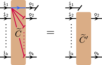
Figure 15: Multipartite non-signalling channels. Each input party i\textup{{i}}_{\ell} can at most send signals to its corresponding output party o\textup{{o}}_{\ell}. Here, this is depicted for the party i1\textup{{i}}_{1}, where a blue arrow denotes the possibility to send a signal, while the red lines signify that no signal can be sent. Since the party i1\textup{{i}}_{1} can only send signals to o1\textup{{o}}_{1}, discarding said outcome then amounts to directly discarding the input i1\textup{{i}}_{1} (depicted in the figure). In terms of the Choi state CC of C~\widetilde{C}, this corresponds to the requirement Co1=Ci1o1{}_{\textup{{o}}_{1}}C={}_{\textup{{i}}_{1}\textup{{o}}_{1}}C of Eq. (148) and analogously for all other pairs {i,o}\{\textup{{i}}_{\ell},\textup{{o}}_{\ell}\}.

Informally, non-signalling channels are multipartite quantum channels which cannot be used for exchanging information between distinct parties. Let kk\in\mathbb{N} be an integer. The Hilbert spaces corresponding to the total input and output, respectively, of such a non-signalling map are given by

i:=\displaystyle\mathcal{H}_{\textup{{i}}}:= i1i2ik\displaystyle\mathcal{H}_{\textup{{i}}_{1}}\otimes\mathcal{H}_{\textup{{i}}_{2}}\otimes\ldots\otimes\mathcal{H}_{\textup{{i}}_{k}} (146)
o:=\displaystyle\mathcal{H}_{\textup{{o}}}:= o1o2ok.\displaystyle\mathcal{H}_{\textup{{o}}_{1}}\otimes\mathcal{H}_{\textup{{o}}_{2}}\otimes\ldots\otimes\mathcal{H}_{\textup{{o}}_{k}}. (147)

Then, a multipartite quantum channel C~:(i)(o)\widetilde{C}:\mathcal{L}(\mathcal{H}_{\textup{{i}}})\to\mathcal{L}(\mathcal{H}_{\textup{{o}}}) is non-signalling if its Choi state CC respects,

(C)o=ioC,{1,2,,k}.{}_{\textup{{o}}_{\ell}}(C)=_{\textup{{i}}_{\ell}\textup{{o}}_{\ell}}C,\quad\forall\ell\in\{1,2,\ldots,k\}. (148)

Intuitively, the above property implies that discarding the output of party \ell amounts to directly discarding its input, which implies that the only signalling of party \ell happens from i\textup{{i}}_{\ell} to o\textup{{o}}_{\ell}, but not to any other output o\textup{{o}}_{\ell^{\prime}} (see Fig. 15 for a graphical depiction).

The requirements of Eq. (148) are equivalent to stating that the map C~:(i)(o)\widetilde{C}:\mathcal{L}(\mathcal{H}_{\textup{{i}}})\to\mathcal{L}(\mathcal{H}_{\textup{{o}}}) can be written as an affine combination of independent channels, that is C~=αγ(α)C~(α)1C~2(α)C~k(α)\widetilde{C}=\sum_{\alpha}\gamma^{(\alpha)}\widetilde{C}^{{(\alpha)}_{1}}\otimes\widetilde{C}^{(\alpha)}_{2}\otimes\ldots\otimes\widetilde{C}^{(\alpha)}_{k}, where γ(α)\gamma^{(\alpha)}\in\mathbb{R}, αγ(α)=1\sum_{\alpha}\gamma^{(\alpha)}=1, and all maps C~(α):(i)(o)\widetilde{C}^{(\alpha)}_{\ell}:\mathcal{L}(\mathcal{H}_{\textup{{i}}_{\ell}})\to\mathcal{L}(\mathcal{H}_{\textup{{o}}_{\ell}}) are quantum channels [34, 35].

From this, we obtain a simple characterisation of non-signalling quantum channels. To this end, we define the projectors:

P~()\displaystyle\widetilde{P}^{(\ell)} :(io)(io),\displaystyle:\mathcal{L}(\mathcal{H}_{\textup{{i}}_{\ell}}\otimes\mathcal{H}_{\textup{{o}}_{\ell}})\to\mathcal{L}(\mathcal{H}_{\textup{{i}}_{\ell}}\otimes\mathcal{H}_{\textup{{o}}_{\ell}}), {1,2,,k},\displaystyle\ell\in\{1,2,\ldots,k\}, (149)
P~()[C]\displaystyle\widetilde{P}^{(\ell)}[C] :=CoC+ioC,\displaystyle:=C-_{\textup{{o}}_{\ell}}C+_{\textup{{i}}_{\ell}\textup{{o}}_{\ell}}C, {1,2,,k},\displaystyle\ell\in\{1,2,\ldots,k\}, (150)
P~NS\displaystyle\widetilde{P}_{NS} :(io)(io),\displaystyle:\mathcal{L}(\mathcal{H}_{\textup{{i}}}\otimes\mathcal{H}_{\textup{{o}}})\to\mathcal{L}(\mathcal{H}_{\textup{{i}}}\otimes\mathcal{H}_{\textup{{o}}}), (151)
P~NS\displaystyle\widetilde{P}_{NS} :=P~(k)P~(2)P~(1).\displaystyle:=\widetilde{P}^{(k)}\circ\ldots\circ\widetilde{P}^{(2)}\circ\widetilde{P}^{(1)}. (152)

We emphasise that, here, the order in which the projectors P~()\widetilde{P}^{(\ell)} are applied in Eq. (152) does not matter, since they all commute (making a construction of P~NS\widetilde{P}_{NS} via concatenation possible in the first place). Hence, a linear operator C(io)C\in\mathcal{L}(\mathcal{H}_{\textup{{i}}}\otimes\mathcal{H}_{\textup{{o}}}) is a non-signalling quantum channel if and only if

C0\displaystyle C\geq 0 (153)
P~NS[C]=C\displaystyle\widetilde{P}_{NS}[C]=C (154)
tr[C]=do.\displaystyle\tr[C]=d_{\textup{{o}}}. (155)

Since the multipartite process matrices lie in the dual affine set of non-signalling channels, Thm. 3 provides a simple characterisation of multipartite process matrices for an arbitrary number of parties.

Example 12 (Multipartite process matrices).

Using the projectors for multipartite non-signalling channels defined in Eqs. (150) and (152) and Thm. 3, we obtain a simple characterisation for multipartite process matrices for any numbers of parties kk.

   
(Multipartite non-signalling channel) (Complex number)
C(io)C\in\mathcal{L}(\mathcal{H}_{\textup{{i}}}\otimes\mathcal{H}_{\textup{{o}}}) belongs to 𝒮i\mathcal{S}_{\textup{{i}}} iff c()c\in\mathcal{L}(\mathbb{C}) belongs to 𝒮o\mathcal{S}_{\textup{{o}}} iff
C0C\geq 0, c0c\geq 0,
C=P~NS[C]C=\widetilde{P}_{NS}[C], \mathbf{\longrightarrow} P~o[c]:=c\widetilde{P}_{\textup{{o}}}[c]:=c,
tr[C]=di\tr[C]=d_{\textup{{i}}}. tr[c]=1\tr[c]=1.
(Multipartite process matrix)
W\displaystyle W\geq 0,\displaystyle 0, (161a)
W=WP~NS[W]\displaystyle W=W-\widetilde{P}_{NS}[W] +tr[W]𝟙iodido,\displaystyle+\tr[W]\frac{\mathds{1}_{\textup{{i}}\textup{{o}}}}{d_{\textup{{i}}}d_{\textup{{o}}}}, (161b)
tr[W]=\displaystyle\tr[W]= do.\displaystyle d_{\textup{{o}}}\,. (161c)

We emphasise that this characterisation of multi-partite process matrices has also been provided in equivalent form in App. B3 of Ref. [15]. Here, it follows straightforwardly from the (readily derived) properties of non-signalling channels, and the fact that process matrices form their dual affine set. \blacksquare

8 Link product and key concepts

The proofs of Thm. 2 as well as its generalisations rely on only a handful of simple mathematical concepts, which we now discuss. Predominantly, we will rely on three main ingredients: The Choi-Jamiołkowski isomorphism (CJI), which allows us to phrase all statements on maps in terms of matrices; the link product, which translates the concatenation of maps to the corresponding manipulation on the level of Choi matrices; and the fact that linear operators with particular properties can be moved around freely in the link product.

8.1 Link Product

We start by discussing the link product \star, already informally introduced in Eq. (25), which captures the action of maps in terms of the CJI [5]. Concretely, for any linear maps T~xy:(x)(y)\widetilde{T}_{\texttt{x}\texttt{y}}:\mathcal{L}(\mathcal{H}_{\texttt{x}})\rightarrow\mathcal{L}(\mathcal{H}_{\texttt{y}}), V~yz:(y)(z)\widetilde{V}_{\texttt{y}\texttt{z}}:\mathcal{L}(\mathcal{H}_{\texttt{y}})\rightarrow\mathcal{L}(\mathcal{H}_{\texttt{z}}) and arbitrary matrices Mx(x)M_{\texttt{x}}\in\mathcal{L}(\mathcal{H}_{\texttt{x}}), we have

Choi[T~yzV~xy]=:VyzTxy(xz)andT~xy[Mx]=TxyMx(y),\displaystyle\text{Choi}[\widetilde{T}_{\texttt{y}\texttt{z}}\circ\widetilde{V}_{\texttt{x}\texttt{y}}]=:V_{\texttt{y}\texttt{z}}\star T_{\texttt{x}\texttt{y}}\in\mathcal{L}(\mathcal{H}_{\texttt{x}}\otimes\mathcal{H}_{\texttt{z}})\quad\text{and}\quad\widetilde{T}_{\texttt{x}\texttt{y}}[M_{\texttt{x}}]=T_{\texttt{x}\texttt{y}}\star M_{\texttt{x}}\in\mathcal{L}(\mathcal{H}_{\texttt{y}})\,, (162)

where Choi[    ]\text{Choi}[\,\begin{picture}(-1.0,-3.0)\circle*{3.0}\end{picture}\ \,] transforms a map to its corresponding Choi matrix. In particular, the link product of two arbitrary matrices Txy:(xy)T_{\texttt{x}\texttt{y}}:\mathcal{L}(\mathcal{H}_{\texttt{x}}\otimes\mathcal{H}_{\texttt{y}}) and Vyz:(yz)V_{\texttt{y}\texttt{z}}:\mathcal{L}(\mathcal{H}_{\texttt{y}}\otimes\mathcal{H}_{\texttt{z}}) is given by a trace over the spaces they are both defined on and a partial transpose over the same space2121 21 The concrete form of the link product – in particular the presence of partial transposes – depends on the convention of the CJI one employs. The form of the link product we present here is in line with the convention chosen in Eq. (1)., i.e.,

TxyVyz:=trz[(Txy𝟙z)(𝟙xVyzτy)],\displaystyle T_{\texttt{x}\texttt{y}}\star V_{\texttt{y}\texttt{z}}:=\tr_{\texttt{z}}[(T_{\texttt{x}\texttt{y}}\otimes\mathbbm{1}_{\texttt{z}})(\mathbbm{1}_{\texttt{x}}\otimes V_{\texttt{y}\texttt{z}}^{\tau_{\texttt{y}}})]\,, (163)

where     τy\,\begin{picture}(-1.0,-3.0)\circle*{3.0}\end{picture}\ ^{\tau_{\texttt{y}}} denotes the partial transpose with respect to the computational basis of y\mathcal{H}_{\texttt{y}}. As has been shown in Refs. [5], the link product of positive semidefinite (Hermitian) matrices is again positive semidefinite (Hermitian), and it is both associative and – for all cases we consider – commutative (up to a re-ordering of tensor factors, which we always tacitly assume). Additionally, it is easy to see that the link product satisfies

AB=ABBA=A,\displaystyle A\star B=A^{\prime}\star B\quad\forall B\quad\Leftrightarrow\quad A=A^{\prime}, (164)

since ABA\star B and ABA^{\prime}\star B are equal to A~[B]\widetilde{A}[B] and A~[B]\widetilde{A}^{\prime}[B], respectively, and if two linear maps agree on all elements they act on, they coincide, i.e., A~=A~\widetilde{A}=\widetilde{A}^{\prime} and thus A=AA=A^{\prime} (the converse direction in Eq. (164) holds trivially).

Importantly, the link product allows us to re-phrase the question of finding the properties of (trace-rescaling) mappings T~io\widetilde{T}_{\textup{{i}}\textup{{o}}} between sets 𝒮i\mathcal{S}_{\textup{{i}}} and 𝒮o\mathcal{S}_{\textup{{o}}} defined by projectors P~i\widetilde{P}_{\textup{{i}}} and P~o\widetilde{P}_{\textup{{o}}}, respectively, in terms of Choi matrices. The requirements that T~io[Wi]𝒮o\widetilde{T}_{\textup{{i}}\textup{{o}}}[W_{\textup{{i}}}]\in\mathcal{S}_{\textup{{o}}} and tr[T~io[Wi]]=γo/γitr[Wi]\tr[\widetilde{T}_{\textup{{i}}\textup{{o}}}[W_{\textup{{i}}}]]=\gamma_{\textup{{o}}}/\gamma_{\textup{{i}}}\tr[W_{\textup{{i}}}] for all Wi𝒮iW_{\textup{{i}}}\in\mathcal{S}_{\textup{{i}}} can now be phrased as

(𝟙~iP~o)[TioWi]=TioWiandtr[TioWi]=γoγitr[Wi]\displaystyle(\widetilde{\mathds{1}}_{\textup{{i}}}\otimes\widetilde{P}_{\textup{{o}}})[T_{\textup{{i}}\textup{{o}}}\star W_{\textup{{i}}}]=T_{\textup{{i}}\textup{{o}}}\star W_{\textup{{i}}}\quad\text{and}\quad\tr[T_{\textup{{i}}\textup{{o}}}\star W_{\textup{{i}}}]=\frac{\gamma_{\textup{{o}}}}{\gamma_{\textup{{i}}}}\tr[W_{\textup{{i}}}] (165)

for all Wi=P~[Wi]W_{\textup{{i}}}=\widetilde{P}[W_{\textup{{i}}}] and tr[Wi]=γi\tr[W_{\textup{{i}}}]=\gamma_{\textup{{i}}}. In order to deduce the structural properties these two equations engender for TioT_{\textup{{i}}\textup{{o}}}, all constraints need to be ‘moved onto’ TioT_{\textup{{i}}\textup{{o}}}. Consequently, we now discuss how to ‘move around’ linear maps in the link product.

8.2 Linear operators in the link product

The final property of the link product that we will make frequent use of is the fact that linear maps that act on one of the factors in the link product can be ‘moved around’(this is akin to finding their adjoint action). In order to obtain simplifications for the special case of self-adjoint, unital maps that commute with the transposition – the case most frequently encountered in quantum mechanics – we first recall some (well-known) pertinent properties of such maps:

Lemma 4 (Properties of linear maps).

Let P~:()()\widetilde{P}:\mathcal{L}(\mathcal{H})\rightarrow\mathcal{L}(\mathcal{H}) be a linear map. The following statements hold:

  1. 1.

    If P~\widetilde{P} is self-adjoint, then it is Hermiticity preserving.

  2. 2.

    If P~\widetilde{P} is self-adjoint and unital, then it is trace-preserving.

  3. 3.

    If P~\widetilde{P} is self-adjoint, then it commutes with the transposition iff it commutes with complex conjugation (with respect to the same basis).

  4. 4.

    If P~\widetilde{P} is self-adjoint and commutes with the transposition (or complex conjugation), then tr[MP~[M]]=tr[P~[M]M]\tr[M^{\prime}\widetilde{P}[M]]=\tr[\widetilde{P}[M^{\prime}]M] for all M,M()M^{\prime},M\in\mathcal{L}(\mathcal{H}).

  5. 5.

    If P~\widetilde{P} is Hermiticity preserving, then tr[HP~[H]]=tr[P~[H]H]\tr[H^{\prime}\widetilde{P}[H]]=\tr[\widetilde{P}[H^{\prime}]H] for all Hermitian H,H()H^{\prime},H\in\mathcal{L}(\mathcal{H}).

All the proofs follow by direct insertion and are provided in App. C for completeness. With these properties of linear maps P~\widetilde{P} in hand, we can now investigate how linear maps can be ‘moved around’ in the link product.

Lemma 5.

Let Aio(io)A_{\textup{{{i}}}\textup{{{o}}}}\in\mathcal{L}(\mathcal{H}_{\textup{{{i}}}}\otimes\mathcal{H}_{\textup{{{o}}}}) and Bi(i)B_{\textup{{{i}}}}\in\mathcal{L}(\mathcal{H}_{\textup{{{i}}}}), and let P~i:(i)(i)\widetilde{P}_{\textup{{{i}}}}:\mathcal{L}(\mathcal{H}_{\textup{{{i}}}})\rightarrow\mathcal{L}(\mathcal{H}_{\textup{{{i}}}}) be a linear operator. Then

AioP~i[Bi]=P~i[Aio]Bi=:P~iτ[Aio]Bi.\displaystyle A_{\textup{{{i}}}\textup{{{o}}}}\star\widetilde{P}_{\textup{{{i}}}}[B_{\textup{{{i}}}}]=\widetilde{P}^{\dagger}_{\textup{{{i}}}}[A^{*}_{\textup{{{i}}{{o}}}}]^{*}\star B_{\textup{{i}}}=:\widetilde{P}_{\textup{{{i}}}}^{\tau}[A_{\textup{{{i}}{{o}}}}]\star B_{\textup{{{i}}}}. (166)

If P~i\widetilde{P}_{\textup{{{i}}}} is self-adjoint and commutes with the transposition (or complex conjugation), then

AioP~i[Bi]=P~i[Aio]Bi\displaystyle A_{\textup{{{i}}}\textup{{{o}}}}\star\widetilde{P}_{\textup{{{i}}}}[B_{\textup{{{i}}}}]=\widetilde{P}_{\textup{{i}}}[A_{\textup{{{i}}{{o}}}}]\star B_{\textup{{{i}}}} (167)

holds.

Proof.

First, we note that, if Eq. (166) holds, then, due to the properties provided in Lem. 4, Eq. (167) follows directly when P~\widetilde{P} is self-adjoint and commutes with the transposition (or complex conjugation). For the proof of Eq. (166), we first recall that the action of any linear operator P~i:(i)(i)\widetilde{P}_{\textup{{i}}}:\mathcal{L}(\mathcal{H}_{\textup{{i}}})\rightarrow\mathcal{L}(\mathcal{H}_{\textup{{i}}}) can be written as P~i[    ]=αLi(α)    Ri(α)\widetilde{P}_{\textup{{i}}}[\,\begin{picture}(-1.0,-3.0)\circle*{3.0}\end{picture}\ \,]=\sum_{\alpha}L^{(\alpha)}_{\textup{{i}}}\,\begin{picture}(-1.0,-3.0)\circle*{3.0}\end{picture}\ \,R^{(\alpha)\dagger}_{\textup{{i}}} for some matrices L(α)i,R(α)iiL^{(\alpha)}_{\textup{{i}}},R^{(\alpha)\dagger}_{\textup{{i}}}\in\mathcal{H}_{\textup{{i}}}. With this, from the definition of the adjoint, it is easy to see that P~i[    ]=αLi(α)    Ri(α)\widetilde{P}_{\textup{{i}}}^{\dagger}[\,\begin{picture}(-1.0,-3.0)\circle*{3.0}\end{picture}\ \,]=\sum_{\alpha}L_{\textup{{i}}}^{(\alpha)\dagger}\,\begin{picture}(-1.0,-3.0)\circle*{3.0}\end{picture}\ \,R_{\textup{{i}}}^{(\alpha)} holds. Now, using the definition of the link product, we obtain

AioP~i[Bi]\displaystyle A_{\textup{{{i}}}\textup{{{o}}}}\star\widetilde{P}_{\textup{{{i}}}}[B_{\textup{{{i}}}}] =tri[Aio(P~i[Bi]τ𝟙o)]=αtri[Aio(Ri(α)BiτLi(α)τ𝟙o)]\displaystyle=\tr_{\textup{{{i}}}}[A_{\textup{{{i}}{{o}}}}(\widetilde{P}_{\textup{{{i}}}}[B_{\textup{{{i}}}}]^{\tau}\otimes\mathbbm{1}_{\textup{{{o}}}})]=\sum_{\alpha}\tr_{\textup{{{i}}}}[A_{\textup{{{i}}{{o}}}}(R_{\textup{{i}}}^{(\alpha)*}B_{\textup{{{i}}}}^{\tau}L_{\textup{{i}}}^{(\alpha)\tau}\otimes\mathbbm{1}_{\textup{{{o}}}})] (168)
=αtri[(Li(α)AioRi(α))(Biτ𝟙o)]=P~i[Aio]Bi,\displaystyle=\sum_{\alpha}\tr_{\textup{{{i}}}}[(L_{\textup{{i}}}^{(\alpha)\dagger}A_{\textup{{{i}}{{o}}}}^{*}R_{\textup{{i}}}^{(\alpha)})^{*}(B_{\textup{{{i}}}}^{\tau}\otimes\mathbbm{1}_{\textup{{{o}}}})]=\widetilde{P}^{\dagger}_{\textup{{i}}}[A^{*}_{\textup{{i}}\textup{{o}}}]^{*}\star B_{\textup{{i}}}\,, (169)

We note that it is easy to see that, if P~i[    ]=αLi(α)    Ri(α)\widetilde{P}_{\textup{{i}}}[\,\,\begin{picture}(-1.0,-3.0)\circle*{3.0}\end{picture}\ \,]=\sum_{\alpha}L_{\textup{{i}}}^{(\alpha)}\,\begin{picture}(-1.0,-3.0)\circle*{3.0}\end{picture}\ \,R_{\textup{{i}}}^{(\alpha)\dagger}, then P~iτ[    ]:=Pi[    ]=Li(α)τ    Ri(α)\widetilde{P}_{\textup{{i}}}^{\tau}[\,\,\begin{picture}(-1.0,-3.0)\circle*{3.0}\end{picture}\ \,]:=P^{\dagger}_{\textup{{i}}}[\,\,\begin{picture}(-1.0,-3.0)\circle*{3.0}\end{picture}\ ^{*}]^{*}=L_{\textup{{i}}}^{(\alpha)\tau}\,\begin{picture}(-1.0,-3.0)\circle*{3.0}\end{picture}\ \,R_{\textup{{i}}}^{(\alpha)*}. Importantly for our purposes, Eqs. (166) and (167) allow us to move linear operators around freely in the link product, which we will now exploit to deduce the properties of TioT_{\textup{{i}}\textup{{o}}}.

8.3 Proving statements using the link product

Now, using the link product, we can easily provide the proofs for the statements made in Secs. 3 and 7. As mentioned, for any linear map T~io\widetilde{T}_{\textup{{i}}\textup{{o}}} that maps 𝒮i\mathcal{S}_{\textup{{i}}} onto 𝒮o\mathcal{S}_{\textup{{o}}}, we have

(𝟙~iP~o)[TioWi]=TioWiandtr[TioWi]=γoγitr[Wi]Wi𝒮i\displaystyle(\widetilde{\mathds{1}}_{\textup{{i}}}\otimes\widetilde{P}_{\textup{{o}}})[T_{\textup{{i}}\textup{{o}}}\star W_{\textup{{i}}}]=T_{\textup{{i}}\textup{{o}}}\star W_{\textup{{i}}}\quad\text{and}\quad\tr[T_{\textup{{i}}\textup{{o}}}\star W_{\textup{{i}}}]=\frac{\gamma_{\textup{{o}}}}{\gamma_{\textup{{i}}}}\tr[W_{\textup{{i}}}]\quad\forall W_{\textup{{i}}}\in\mathcal{S}_{\textup{{i}}} (170)

Let us start by providing the structural properties of TioT_{\textup{{i}}\textup{{o}}} for the case of self-adjoint, unital projectors P~i\widetilde{P}_{\textup{{i}}} and P~o\widetilde{P}_{\textup{{o}}} that commute with the transposition. To do so, we first make use of (𝟙~iP~o)[TioWi]=(𝟙~iP~o)[Tio]Wi=TioWi(\widetilde{\mathds{1}}_{\textup{{i}}}\otimes\widetilde{P}_{\textup{{o}}})[T_{\textup{{i}}\textup{{o}}}\star W_{\textup{{i}}}]=(\widetilde{\mathds{1}}_{\textup{{i}}}\otimes\widetilde{P}_{\textup{{o}}})[T_{\textup{{i}}\textup{{o}}}]\star W_{\textup{{i}}}=T_{\textup{{i}}\textup{{o}}}\star W_{\textup{{i}}} for all Wi𝒮iW_{\textup{{i}}}\in\mathcal{S}_{\textup{{i}}}. Importantly, since span(𝒮i)\text{span}(\mathcal{S}_{\textup{{i}}}) does generally not coincide with the full space (i)\mathcal{L}(\mathcal{H}_{\textup{{i}}}), this equation does not allow us to deduce that (𝟙~iP~o)[Tio]=Tio(\widetilde{\mathds{1}}_{\textup{{i}}}\otimes\widetilde{P}_{\textup{{o}}})[T_{\textup{{i}}\textup{{o}}}]=T_{\textup{{i}}\textup{{o}}}. However, it is easy to see (since P~i\widetilde{P}_{\textup{{i}}} is a projection) that for every M(i)M\in\mathcal{L}(\mathcal{H}_{\textup{{i}}}) with tr[W]0\tr[W]\neq 0 (for the case γi=0\gamma_{\textup{{i}}}=0 see App. B) we have P~i[M]span(𝒮i)\widetilde{P}_{\textup{{i}}}[M]\in\text{span}(\mathcal{S}_{\textup{{i}}}). Consequently, we obtain

(𝟙~iP~o)[Tio]P~i[M]=TioP~i[M]M(i)\displaystyle(\widetilde{\mathds{1}}_{\textup{{i}}}\otimes\widetilde{P}_{\textup{{o}}})[T_{\textup{{i}}\textup{{o}}}]\star\widetilde{P}_{\textup{{i}}}[M]=T_{\textup{{i}}\textup{{o}}}\star\widetilde{P}_{\textup{{i}}}[M]\quad\forall M\in\mathcal{L}(\mathcal{H}_{\textup{{i}}}) (171)

Now, we can use the second part of Lem. 5 to move the projector P~i\widetilde{P}_{\textup{{i}}} inside the link product, such that

(P~iP~o)[Tio]M=P~i[Tio]MM(i),\displaystyle(\widetilde{P}_{\textup{{i}}}\otimes\widetilde{P}_{\textup{{o}}})[T_{\textup{{i}}\textup{{o}}}]\star M=\widetilde{P}_{\textup{{i}}}[T_{\textup{{i}}\textup{{o}}}]\star M\quad\forall M\in\mathcal{L}(\mathcal{H}_{\textup{{i}}})\,, (172)

which, since it holds for all M(i)M\in\mathcal{L}(\mathcal{H}_{\textup{{i}}}), implies (P~iP~o)[Tio]=P~i[Tio](\widetilde{P}_{\textup{{i}}}\otimes\widetilde{P}_{\textup{{o}}})[T_{\textup{{i}}\textup{{o}}}]=\widetilde{P}_{\textup{{i}}}[T_{\textup{{i}}\textup{{o}}}]. This, in turn, can be phrased in terms of a projector on TioT_{\textup{{i}}\textup{{o}}} as

Tio=TioP~i[Tio]+(P~iP~o)[Tio],\displaystyle T_{\textup{{i}}\textup{{o}}}=T_{\textup{{i}}\textup{{o}}}-\widetilde{P}_{\textup{{i}}}[T_{\textup{{i}}\textup{{o}}}]+(\widetilde{P}_{\textup{{i}}}\otimes\widetilde{P}_{\textup{{o}}})[T_{\textup{{i}}\textup{{o}}}]\,, (173)

where the signs in the above definition are chosen such that P~i[Tio]=(P~iP~o)[Tio]\widetilde{P}_{\textup{{i}}}[T_{\textup{{i}}\textup{{o}}}]=(\widetilde{P}_{\textup{{i}}}\otimes\widetilde{P}_{\textup{{o}}})[T_{\textup{{i}}\textup{{o}}}] still holds (which can be seen by direct insertion into (173) and using that P~i\widetilde{P}_{\textup{{i}}} is a projector).

In a similar vein, we can analyse the trace-rescaling property tr[TioWi]=γo/γitr[W]\tr[T_{\textup{{i}}\textup{{o}}}\star W_{\textup{{i}}}]=\gamma_{\textup{{o}}}/\gamma_{\textup{{i}}}\tr[W] for all W𝒮iW\in\mathcal{S}_{\textup{{i}}}. Following the same argument (and using the fact that 𝟙i\mathbbm{1}_{\textup{{i}}} is the Choi state of tri\tr_{\textup{{i}}}), we obtain

P~i[troTio]M=γoγi𝟙iM.\displaystyle\widetilde{P}_{\textup{{i}}}[\tr_{\textup{{o}}}T_{\textup{{i}}\textup{{o}}}]\star M=\frac{\gamma_{\textup{{o}}}}{\gamma_{\textup{{i}}}}\mathbbm{1}_{\textup{{i}}}\star M\,. (174)

Again, this equality holds for all M(i)M\in\mathcal{L}(\mathcal{H}_{\textup{{i}}}), and thus implies

P~i[troTio]=γoγi𝟙i.\displaystyle\widetilde{P}_{\textup{{i}}}[\tr_{\textup{{o}}}T_{\textup{{i}}\textup{{o}}}]=\frac{\gamma_{\textup{{o}}}}{\gamma_{\textup{{i}}}}\mathbbm{1}_{\textup{{i}}}\,. (175)

Since P~i\widetilde{P}_{\textup{{i}}} is unital and self-adjoint, it is trace-preserving (see Lem. 4), and we see that tr[Tio]=γo/γidi\tr[T_{\textup{{i}}\textup{{o}}}]=\gamma_{\textup{{o}}}/\gamma_{\textup{{i}}}\cdot d_{\textup{{i}}}. With this, by taking the tensor product of Eq. (175) with 𝟙o/do\mathbbm{1}_{\textup{{o}}}/d_{\textup{{o}}}, we obtain P~i[Tioo]=Tioio\widetilde{P}_{\textup{{i}}}[{}_{\textup{{o}}}T_{\textup{{i}}\textup{{o}}}]={}_{\textup{{i}}\textup{{o}}}T_{\textup{{i}}\textup{{o}}}, such that Eqs (175) and (174) can equivalently be written as

Tio=TioP~i[Tioo]+Tioioandtr[Tio]=γoγidi.\displaystyle T_{\textup{{i}}\textup{{o}}}=T_{\textup{{i}}\textup{{o}}}-\widetilde{P}_{\textup{{i}}}[{}_{\textup{{o}}}T_{\textup{{i}}\textup{{o}}}]+{}_{\textup{{i}}\textup{{o}}}T_{\textup{{i}}\textup{{o}}}\,\quad\text{and}\quad\tr[T_{\textup{{i}}\textup{{o}}}]=\frac{\gamma_{\textup{{o}}}}{\gamma_{\textup{{i}}}}d_{\textup{{i}}}\,. (176)

Now, inserting this into Eq. (173), we obtain

Tio=TioP~i[Tio]+(P~iP~o)[Tio]P~i[Tioo]+Tioio=:P~io[Tio]andtr[Tio]=γoγidi,\displaystyle T_{\textup{{i}}\textup{{o}}}=T_{\textup{{i}}\textup{{o}}}-\widetilde{P}_{\textup{{i}}}[T_{\textup{{i}}\textup{{o}}}]+(\widetilde{P}_{\textup{{i}}}\otimes\widetilde{P}_{\textup{{o}}})[T_{\textup{{i}}\textup{{o}}}]-\widetilde{P}_{\textup{{i}}}[{}_{\textup{{o}}}T_{\textup{{i}}\textup{{o}}}]+{}_{\textup{{i}}\textup{{o}}}T_{\textup{{i}}\textup{{o}}}=:\widetilde{P}_{\textup{{i}}\textup{{o}}}[T_{\textup{{i}}\textup{{o}}}]\quad\text{and}\quad\tr[T_{\textup{{i}}\textup{{o}}}]=\frac{\gamma_{\textup{{o}}}}{\gamma_{\textup{{i}}}}d_{\textup{{i}}}\,, (177)

which coincides exactly with Eqs. (30a) and (30b) of Thm. 2. For the converse direction, we first note that a self-adjoint, unital projector P~o\widetilde{P}_{\textup{{o}}} is trace-preserving, such that P~o[Mo]=oP~o[M]=Mo\widetilde{P}_{\textup{{o}}}[{}_{\textup{{o}}}M]={}_{\textup{{o}}}\circ\widetilde{P}_{\textup{{o}}}[M]={}_{\textup{{o}}}M holds. With this, by direct insertion, it is easy to see that Eq. (177) implies P~i[Tioo]=Tioio\widetilde{P}_{\textup{{i}}}[{}_{\textup{{o}}}T_{\textup{{i}}\textup{{o}}}]={}_{\textup{{i}}\textup{{o}}}T_{\textup{{i}}\textup{{o}}} and thus Eqs. (176) and (173); together with Eq. (177), these latter two equations directly lead to Eq. (170), thus proving Thm. 2. We emphasise, that this converse direction crucially requires the properties of P~o\widetilde{P}_{\textup{{o}}} (i.e., self-adjointness and unitality), while the forward direction also holds without these assumptions on P~o\widetilde{P}_{\textup{{o}}}.

Finally, if we dropped the trace-rescaling property on T~io\widetilde{T}_{\textup{{i}}\textup{{o}}} (and thus TioT_{\textup{{i}}\textup{{o}}}), such that we only demand P~o[TioWi]=TioWi\widetilde{P}_{\textup{{o}}}[T_{\textup{{i}}\textup{{o}}}\star W_{\textup{{i}}}]=T_{\textup{{i}}\textup{{o}}}\star W_{\textup{{i}}} for all Wi=P~i[Wi]W_{\textup{{i}}}=\widetilde{P}_{\textup{{i}}}[W_{\textup{{i}}}](but not tr[TioWi]=γoγitr[Wi]\tr[T_{\textup{{i}}\textup{{o}}}\star W_{\textup{{i}}}]=\frac{\gamma_{\textup{{o}}}}{\gamma_{\textup{{i}}}}\tr[W_{\textup{{i}}}]), following the above derivation, we arrive at

Theorem 4 (Transformation between linear spaces: specialised Choi version).

Let P~i:(i)(i)\widetilde{P}_{\textup{{i}}}:\mathcal{L}(\mathcal{H}_{\textup{{i}}})\to\mathcal{L}(\mathcal{H}_{\textup{{i}}}) and P~o:(o)(o)\widetilde{P}_{\textup{{o}}}:\mathcal{L}(\mathcal{H}_{\textup{{o}}})\to\mathcal{L}(\mathcal{H}_{\textup{{o}}}) be linear projective, self-adjoint and unital maps that commute with the transposition (or conjugation) and 𝒮i(i)\mathcal{S}_{\textup{{i}}}\subseteq\mathcal{L}(\mathcal{H}_{\textup{{i}}}) and 𝒮o(o)\mathcal{S}_{\textup{{o}}}\subseteq\mathcal{L}(\mathcal{H}_{\textup{{o}}}) be linear spaces defined by

W(i)W\in\mathcal{L}(\mathcal{H}_{\textup{{i}}}) belongs to 𝒮i\mathcal{S}_{\textup{{i}}} iff \mathbf{\longrightarrow} W(o)W^{\prime}\in\mathcal{L}(\mathcal{H}_{\textup{{o}}}) belongs to 𝒮o\mathcal{S}_{\textup{{o}}} iff
P~i[W]=W\widetilde{P}_{\textup{{i}}}[W]=W. P~o[W]=W\widetilde{P}_{\textup{{o}}}[W^{\prime}]=W^{\prime}.

A linear map T~io:(i)(o)\widetilde{T}_{\textup{{{i}}{{o}}}}:\mathcal{L}(\mathcal{H}_{\textup{{{i}}}})\rightarrow\mathcal{L}(\mathcal{H}_{\textup{{{o}}}}) satisfies T~io[W]𝒮o,\widetilde{T}_{\textup{{{i}}{{o}}}}[W]\in\mathcal{S}_{\textup{{{o}}}}, for all W𝒮iW\in\mathcal{S}_{\textup{{{i}}}} if and only if

Tio=Tio(P~i𝟙~o)[Tio]+(P~iP~o)[Tio]=:P~io(ntr)[Tio],\displaystyle T_{\textup{{i}}\textup{{o}}}=T_{\textup{{i}}\textup{{o}}}-(\widetilde{P}_{\textup{{i}}}\otimes\widetilde{\mathds{1}}_{\textup{{o}}})[T_{\textup{{i}}\textup{{o}}}]+(\widetilde{P}_{\textup{{i}}}\otimes\widetilde{P}_{\textup{{o}}})[T_{\textup{{i}}\textup{{o}}}]=:\widetilde{P}^{(\textup{ntr})}_{\textup{{i}}\textup{{o}}}[T_{\textup{{i}}\textup{{o}}}]\,, (180)

holds for its Choi matrix TioT_{\textup{{i}}\textup{{o}}}, and P~io(ntr):(io)(io)\widetilde{P}^{(\text{ntr})}_{\textup{{i}}\textup{{o}}}:\mathcal{L}(\mathcal{H}_{\textup{{i}}}\otimes\mathcal{H}_{\textup{{o}}})\to\mathcal{L}(\mathcal{H}_{\textup{{i}}}\otimes\mathcal{H}_{\textup{{o}}}) is a self-adjoint, unital projector that commutes with the transposition.

Proof.

The proof proceeds along the same line as the previous one, minus the additional requirement of a trace-rescaling property, i.e., it stops at Eq. (176), which coincides with Eq. (180) of the Theorem. Conversely, it is easy to see that the above equality implies P~o[TioWi]=TioWi\widetilde{P}_{\textup{{o}}}[T_{\textup{{i}}\textup{{o}}}\star W_{\textup{{i}}}]=T_{\textup{{i}}\textup{{o}}}\star W_{\textup{{i}}} for all Wi=P~i[Wi]W_{\textup{{i}}}=\widetilde{P}_{\textup{{i}}}[W_{\textup{{i}}}], independent of the properties of P~o\widetilde{P}_{\textup{{o}}} (besides being a linear projector), proving Thm. 4. ∎

Importantly, the above Theorem in not simply a special case of Thm. 2, particularly, it does not coincide with it up to the affine constraint, but the respective constraints on TioT_{\textup{{i}}\textup{{o}}} are structurally different. This is a generalisation of the structural differences of, e.g., CP and CPTP maps; the former are not just equal to the latter up to a trace condition, but CPTP maps have an additional structural property, that is absent in CP maps (namely, that the trace over the output degrees of freedom yields the identity matrix on the input space.).

In addition, we note that Thm. 4 covers the case γi=0\gamma_{\textup{{i}}}=0 of Thm. 2. As detailed in App. B, in this case, both γi\gamma_{\textup{{i}}} and γo\gamma_{\textup{{o}}} are equal to zero, such that both spaces 𝒮i\mathcal{S}_{\textup{{i}}} and 𝒮o\mathcal{S}_{\textup{{o}}} are entirely defined by linear projectors onto a vector space of traceless operators, which is a special instance of the scenario discussed in the above theorem.

With this, we have considered all pertinent scenarios including projectors that are self-adjoint, unital, and commute with the transposition. We conclude this paper with the general case, where we impose no constraints on P~i\widetilde{P}_{\textup{{i}}} and P~o\widetilde{P}_{\textup{{o}}}, besides them being linear projectors.

9 General approach

While physically the most relevant case, it is not necessary that the projectors P~i\widetilde{P}_{\textup{{i}}} and P~o\widetilde{P}_{\textup{{o}}} defining the sets 𝒮i\mathcal{S}_{\textup{{i}}} and 𝒮o\mathcal{S}_{\textup{{o}}}, respectively, are self-adjoint, unital, and commute with the transposition. As a guiding example for a case where these properties fail to hold, consider the case where P~i\widetilde{P}_{\textup{{i}}} is given by a projector on the off-diagonal element |mn||m\rangle\hskip-1.13809pt\langle n| (with mnm\neq n), i.e., it acts as P~i[B]=m|B|n|mn|\widetilde{P}_{\textup{{i}}}[B]=\langle m|B|n\rangle|m\rangle\hskip-1.13809pt\langle n|. Naturally, the thusly defined P~i\widetilde{P}_{\textup{{i}}} is a projector (since it satisfies P~i2=P~i\widetilde{P}_{\textup{{i}}}^{2}=\widetilde{P}_{\textup{{i}}}), but it is neither self-adjoint, unital, nor does it commute with the transposition.

To derive the properties of maps T~io\widetilde{T}_{\textup{{i}}\textup{{o}}} between sets defined by such general projectors P~x\widetilde{P}_{\texttt{x}}, we can directly employ Lem. 5, which informs us how to move general linear operators around in the link product. With this, we deduce the concrete form of transformations TioT_{\textup{{i}}\textup{{o}}} in the same vein as the derivation for Thm. 2 provided in Sec. 8.3.

Theorem 5.

Let P~i:(i)(i)\widetilde{P}_{\textup{{i}}}:\mathcal{L}(\mathcal{H}_{\textup{{i}}})\to\mathcal{L}(\mathcal{H}_{\textup{{i}}}) and P~o:(o)(o)\widetilde{P}_{\textup{{o}}}:\mathcal{L}(\mathcal{H}_{\textup{{o}}})\to\mathcal{L}(\mathcal{H}_{\textup{{o}}}) be linear projections and 𝒮i(i)\mathcal{S}_{\textup{{{i}}}}\subseteq\mathcal{L}(\mathcal{H}_{\textup{{{i}}}}) and 𝒮o\mathcal{S}_{\textup{{o}}} be affine spaces of matrices defined by

W(i)W\in\mathcal{L}(\mathcal{H}_{\textup{{i}}}) belongs to 𝒮i\mathcal{S}_{\textup{{i}}} iff W(o)W^{\prime}\in\mathcal{L}(\mathcal{H}_{\textup{{o}}}) belongs to 𝒮o\mathcal{S}_{\textup{{o}}} iff
P~i[W]=W\widetilde{P}_{\textup{{i}}}[W]=W, \mathbf{\longrightarrow} P~o[W]=W\widetilde{P}_{\textup{{o}}}[W^{\prime}]=W^{\prime},
tr[W]=γi\tr[W]=\gamma_{\textup{{i}}}. tr[W]=γo\tr[W^{\prime}]=\gamma_{\textup{{o}}}.

For γi0\gamma_{\textup{{i}}}\neq 0, a linear map T~io:(i)(o)\widetilde{T}_{\textup{{i}}\textup{{o}}}:\mathcal{L}(\mathcal{H}_{\textup{{i}}})\rightarrow\mathcal{L}(\mathcal{H}_{\textup{{o}}}) satisfies T~io[W]𝒮o\widetilde{T}_{\textup{{i}}\textup{{o}}}[W]\in\mathcal{S}_{\textup{{o}}} for all W𝒮iW\in\mathcal{S}_{\textup{{i}}} if and only if

Tio=TioP~iτ[Tio]+(P~iτP~o)[Tio]=:P~io[Tio],\displaystyle T_{\textup{{{i}}{{o}}}}=T_{\textup{{{i}}{{o}}}}-\widetilde{P}_{\textup{{{i}}}}^{\tau}[T_{\textup{{{i}}{{o}}}}]+(\widetilde{P}_{\textup{{{i}}}}^{\tau}\otimes\widetilde{P}_{\textup{{{o}}}})[T_{\textup{{{i}}{{o}}}}]=:\widetilde{P}_{\textup{{i}}\textup{{o}}}[T_{\textup{{{i}}{{o}}}}], (184a)
P~iτ[(troTio)]=γoγiP~iτ[𝟙i].\displaystyle\widetilde{P}_{\textup{{{i}}}}^{\tau}[(\tr_{\textup{{{o}}}}T_{\textup{{{i}}{{o}}}})]=\frac{\gamma_{\textup{{o}}}}{\gamma_{\textup{{i}}}}\widetilde{P}^{\tau}_{\textup{{{i}}}}[\mathbbm{1}_{\textup{{{i}}}}]\,. (184b)

Before providing a proof, we emphasise that the fact that we allow for non-unital, non-self-adjoint projectors implies that the respective sets 𝒮i\mathcal{S}_{\textup{{i}}} and 𝒮o\mathcal{S}_{\textup{{o}}} do not have to contain an element that is proportional to the identity matrix. The membership of the identity matrix facilitates many considerations in the literature when dealing with transformations between quantum objects (see, for example, Ref. [14]). The relative ease with which the link product can be manipulated allows us to go beyond this case without much added difficulty (see Ex. 13).

Furthermore, we stress that the above Theorem exactly coincides with Thm. 2 for the case of self-adjoint, unital projectors P~i\widetilde{P}_{\textup{{i}}} that commute with the transposition. In this case, it is easy to see that Eq. (184a) amounts to Tio=TioP~i[Tio]+(P~iP~o)[Tio]T_{\textup{{i}}\textup{{o}}}=T_{\textup{{{i}}{{o}}}}-\widetilde{P}_{\textup{{{i}}}}[T_{\textup{{{i}}{{o}}}}]+(\widetilde{P}_{\textup{{{i}}}}\otimes\widetilde{P}_{\textup{{{o}}}})[T_{\textup{{{i}}{{o}}}}], while Eq. (184b) implies P~i[troTio]=γo/γi𝟙i\widetilde{P}_{\textup{{i}}}[\tr_{\textup{{o}}}T_{\textup{{i}}\textup{{o}}}]=\gamma_{\textup{{o}}}/\gamma_{\textup{{i}}}\mathbbm{1}_{\textup{{i}}}, which are exactly the properties we used in the proof of Thm. 2.

Proof.

The proof of Thm. 5 proceeds along the same lines as that of Thm. 2 with the difference that now the assumptions on the involved projectors are weaker. First, we note that, since γi0\gamma_{\textup{{i}}}\neq 0, we have span(𝒮i)=P~i[(i)]\text{span}(\mathcal{S}_{\textup{{i}}})=\widetilde{P}_{\textup{{i}}}[\mathcal{L}(\mathcal{H}_{\textup{{i}}})]. Then, from P~o[TioWi]=TioWi\widetilde{P}_{\textup{{o}}}[T_{\textup{{i}}\textup{{o}}}\star W_{\textup{{i}}}]=T_{\textup{{i}}\textup{{o}}}\star W_{\textup{{i}}} for all Wi𝒮iW_{\textup{{i}}}\in\mathcal{S}_{\textup{{i}}} we obtain

P~o[TioP~i[M]]=(P~iτP~o)[Tio]M=TioP~i[M]=P~iτ[Tio]M\displaystyle\widetilde{P}_{\textup{{o}}}[T_{\textup{{i}}\textup{{o}}}\star\widetilde{P}_{\textup{{i}}}[M]]=(\widetilde{P}_{\textup{{i}}}^{\tau}\otimes\widetilde{P}_{\textup{{o}}})[T_{\textup{{i}}\textup{{o}}}]\star M=T_{\textup{{i}}\textup{{o}}}\star\widetilde{P}_{\textup{{i}}}[M]=\widetilde{P}_{\textup{{i}}}^{\tau}[T_{\textup{{i}}\textup{{o}}}]\star M\, (185)

for all M(i)M\in\mathcal{L}(\mathcal{H}_{\textup{{i}}}), where P~iτ\widetilde{P}_{\textup{{i}}}^{\tau} has been defined in Eq. (166). From this, we directly obtain Eq. (184a). From the fact that tr[TioWi]=γo\tr[T_{\textup{{i}}\textup{{o}}}\star W_{\textup{{i}}}]=\gamma_{\textup{{o}}} for all Wi𝒮iW_{\textup{{i}}}\in\mathcal{S}_{\textup{{i}}}, it then follows that tr[TioP~i[M]]=γo/γitr[P~i[M]]\tr[T_{\textup{{i}}\textup{{o}}}\star\widetilde{P}_{\textup{{i}}}[M]]=\gamma_{\textup{{o}}}/\gamma_{\textup{{i}}}\tr[\widetilde{P}_{\textup{{i}}}[M]] for all M(i)M\in\mathcal{L}(\mathcal{H}_{\textup{{i}}}). Using the fact that 𝟙x\mathds{1}_{\texttt{x}} is the Choi matrix of trx\tr_{\texttt{x}}, this can be written as tr[TioP~i[M]]=𝟙iP~i[M]\tr[T_{\textup{{i}}\textup{{o}}}\star\widetilde{P}_{\textup{{i}}}[M]]=\mathds{1}_{\textup{{i}}}\star\widetilde{P}_{\textup{{i}}}[M]. Employing Lem. 5 and using the fact that this equality holds for all M(i)M\in\mathcal{L}(\mathcal{H}_{\textup{{i}}}) then directly yields Eq. (184b). The fact that the resulting linear operator P~io=𝟙~ioP~iτ+P~iτP~o\widetilde{P}_{\textup{{i}}\textup{{o}}}=\widetilde{\mathds{1}}_{\textup{{i}}\textup{{o}}}-\widetilde{P}_{\textup{{i}}}^{\tau}+\widetilde{P}_{\textup{{i}}}^{\tau}\otimes\widetilde{P}_{\textup{{o}}} is indeed a projector can be seen by direct insertion and using the fact that, P~i=P~i2\widetilde{P}_{\textup{{i}}}=\widetilde{P}_{\textup{{i}}}^{2} implies P~iτ=(P~iτ)2\widetilde{P}_{\textup{{i}}}^{\tau}=(\widetilde{P}_{\textup{{i}}}^{\tau})^{2}.

In the converse direction, using P~iτ=(P~iτ)2\widetilde{P}_{\textup{{i}}}^{\tau}=(\widetilde{P}_{\textup{{i}}}^{\tau})^{2}, by direct insertion, it is easy to see that Eq. (184a) implies P~o[TioWi]=TioWi\widetilde{P}_{\textup{{o}}}[T_{\textup{{i}}\textup{{o}}}\star W_{\textup{{i}}}]=T_{\textup{{i}}\textup{{o}}}\star W_{\textup{{i}}} for all Wi𝒮iW_{\textup{{i}}}\in\mathcal{S}_{\textup{{i}}}. ∎

As for the previous Theorems, the case γi=0\gamma_{\textup{{i}}}=0 needs to be discussed in slightly more detail and is provided in App. B.

Example 13 (Gibbs-preserving maps).

To see a concrete application of Thm. 5, consider the case of transformations that have a given fix point, e.g., the Gibbs state η1=exp(βH)/tr[exp(βH)](1)\eta_{1}=\exp{(-\beta H)}/\tr[\exp{(-\beta H)}]\in\mathcal{L}(\mathcal{H}_{1}) for some given inverse temperature β\beta and some Hamiltonian HH. In this case, we have T~[η1]=η2(2)\widetilde{T}[\eta_{1}]=\eta_{2}\in\mathcal{L}(\mathcal{H}_{2}) for some Gibbs state η2\eta_{2}. The projector on the input space is given by P~i[X]=tr[Xη1]η1=:Yη1\widetilde{P}_{\textup{{i}}}[X]=\tr[X\eta_{1}^{\prime}]\eta_{1}^{\prime}=:{}_{\eta_{1}}Y, while the projector on the output space is given by P~o[Y]=tr[Yη2]η2=:Yη2\widetilde{P}_{\textup{{o}}}[Y]=\tr[Y\eta_{2}^{\prime}]\eta_{2}^{\prime}=:{}_{\eta_{2}}Y, where ηx:=ηx/tr[ηx2]\eta_{\textup{{x}}}^{\prime}:=\eta_{\textup{{x}}}/\sqrt{\tr[\eta_{\textup{{x}}}^{2}]} (for x{1,2}\textup{{x}}\in\{1,2\}), and we have γi=γo=1\gamma_{\textup{{i}}}=\gamma_{\textup{{o}}}=1. Assuming that the Choi isomorphism on (1)\mathcal{L}(\mathcal{H}_{1}) is performed with respect to the eigenbasis of η1\eta_{1}, we have P~iτ=P~i\widetilde{P}_{\textup{{i}}}^{\tau}=\widetilde{P}_{\textup{{i}}} and P~iτ[𝟙1]=η1/tr[η12]𝟙1\widetilde{P}_{\textup{{i}}}^{\tau}[\mathds{1}_{1}]=\eta_{1}/\tr[\eta_{1}^{2}]\neq\mathds{1}_{1} for η1𝟙1\eta_{1}\neq\mathds{1}_{1}. Consequently, the projector on the input space is non-unital, and we must apply Thm. 5 (instead of Thm. 2) to deduce the properties of TioT_{\textup{{i}}\textup{{o}}}. Employing Eqs. (184a) and (184b), we obtain

T=TTη1+Tη1η2&tr[T(η1𝟙2)]=1/tr[η12].\displaystyle T=T-{}_{\eta_{1}}T+{}_{\eta_{1}\eta_{2}}T\quad\&\quad\tr[T(\eta_{1}^{\prime}\otimes\mathds{1}_{2})]=1/\sqrt{\tr[\eta_{1}^{2}]}. (186)

These two constraints (together with T0T\geq 0) entirely characterise the set of transformations that leave the Gibbs state invariant. Unsurprisingly, they do not enforce trace preservation (they only guarantee trace preservation on the span of η1\eta_{1}). Adding this as an additional constraint trivialises the second term of the above equation and leads to the following set of trace-preserving Gibbs-preserving transformations:

T=TTη1+Tη1η2=:P~(GP)[T]&T=TTo+Tio=:P~(TP)[T].\displaystyle T=T-{}_{\eta_{1}}T+{}_{\eta_{1}\eta_{2}}T=:\widetilde{P}^{(\mathrm{GP})}[T]\quad\&\quad T=T-{}_{\textup{{o}}}T+{}_{\textup{{i}}\textup{{o}}}T=:\widetilde{P}^{(\mathrm{TP})}[T]. (187)

Since P~(GP)\widetilde{P}^{(\mathrm{GP})} and P~(TP)\widetilde{P}^{(\mathrm{TP})} do not commute, this cannot be further combined into a single projector of the form P~(GP)P~(TP)\widetilde{P}^{(\mathrm{GP})}\circ\widetilde{P}^{(\mathrm{TP})} or P~(TP)P~(GP)\widetilde{P}^{(\mathrm{TP})}\circ\widetilde{P}^{(\mathrm{GP})}. \blacksquare

Similarly to Thm. 4, one can also drop the trace-rescaling property (i.a., the trace constraints on the elements of 𝒮i\mathcal{S}_{\textup{{i}}} and 𝒮o\mathcal{S}_{\textup{{o}}}) for general projectors. In this case, one would simply have to drop Eq. (184b) in the above theorem to obtain the properties of TioT_{\textup{{i}}\textup{{o}}}:

Theorem 6 (Transformation between linear spaces: Choi version).

Let P~i:(i)(i)\widetilde{P}_{\textup{{i}}}:\mathcal{L}(\mathcal{H}_{\textup{{i}}})\to\mathcal{L}(\mathcal{H}_{\textup{{i}}}) and P~o:(o)(o)\widetilde{P}_{\textup{{o}}}:\mathcal{L}(\mathcal{H}_{\textup{{o}}})\to\mathcal{L}(\mathcal{H}_{\textup{{o}}}) be linear projections and 𝒮i(i)\mathcal{S}_{\textup{{{i}}}}\subseteq\mathcal{L}(\mathcal{H}_{\textup{{{i}}}}) and 𝒮o\mathcal{S}_{\textup{{o}}} be linear spaces of matrices defined by

W(i)W\in\mathcal{L}(\mathcal{H}_{\textup{{i}}}) belongs to 𝒮i\mathcal{S}_{\textup{{i}}} iff \mathbf{\longrightarrow} W(o)W^{\prime}\in\mathcal{L}(\mathcal{H}_{\textup{{o}}}) belongs to 𝒮o\mathcal{S}_{\textup{{o}}} iff
P~i[W]=W\widetilde{P}_{\textup{{i}}}[W]=W. P~o[W]=W\widetilde{P}_{\textup{{o}}}[W^{\prime}]=W^{\prime}.

A linear map T~io:(i)(o)\widetilde{T}_{\textup{{i}}\textup{{o}}}:\mathcal{L}(\mathcal{H}_{\textup{{i}}})\rightarrow\mathcal{L}(\mathcal{H}_{\textup{{o}}}) satisfies T~io[W]𝒮o\widetilde{T}_{\textup{{i}}\textup{{o}}}[W]\in\mathcal{S}_{\textup{{o}}} for all W𝒮iW\in\mathcal{S}_{\textup{{i}}} if and only if

Tio=Tio(P~iτ𝟙~o)[Tio]+(P~iτP~o)[Tio]=:P~io[Tio].\displaystyle T_{\textup{{{i}}{{o}}}}=T_{\textup{{{i}}{{o}}}}-(\widetilde{P}_{\textup{{{i}}}}^{\tau}\otimes\widetilde{\mathds{1}}_{\textup{{o}}})[T_{\textup{{{i}}{{o}}}}]+(\widetilde{P}_{\textup{{{i}}}}^{\tau}\otimes\widetilde{P}_{\textup{{{o}}}})[T_{\textup{{{i}}{{o}}}}]=:\widetilde{P}_{\textup{{i}}\textup{{o}}}[T_{\textup{{{i}}{{o}}}}]. (190)

As was the case for Thm. 4, we note again, that this theorem also covers the case γi=0\gamma_{\textup{{i}}}=0 for the case where additional trace constraints are required of 𝒮i\mathcal{S}_{\textup{{i}}} and 𝒮o\mathcal{S}_{\textup{{o}}}(see App. B).

Example 14 (Projectors on off-diagonal terms).

To provide a second concrete example for the above Theorems for the case of projectors that do not preserve Hermiticity, let us return to the simple case mentioned at the beginning of this Section, where P~i\widetilde{P}_{\textup{{{i}}}} is given by a projection on the off-diagonal term |mn||m\rangle\hskip-1.13809pt\langle n| (where mnm\neq n), i.e., it acts as P~i[M]=m|M|n|mn|\widetilde{P}_{\textup{{{i}}}}[M]=\langle m|M|n\rangle|m\rangle\hskip-1.13809pt\langle n|, and let P~o\widetilde{P}_{\textup{{{o}}}} be a projector on the off-diagonal term |αβ|(o)|\alpha\rangle\hskip-1.13809pt\langle\beta|\in\mathcal{L}(\mathcal{H}_{\textup{{{o}}}}), where αβ\alpha\neq\beta. With this, the set 𝒮i\mathcal{S}_{\textup{{{i}}}} consists of all matrices WiW_{\textup{{{i}}}} that are proportional to |mn||m\rangle\hskip-1.13809pt\langle n| and the output space 𝒮o\mathcal{S}_{\textup{{{o}}}} consists of all matrices WoW_{\textup{{{o}}}} that are proportional to |αβ||\alpha\rangle\hskip-1.13809pt\langle\beta| (by construction, all elements of 𝒮i\mathcal{S}_{\textup{{i}}} and 𝒮o\mathcal{S}_{\textup{{o}}} are traceless automatically due to the properties of P~i\widetilde{P}_{\textup{{i}}} and P~o\widetilde{P}_{\textup{{o}}}). It is easy to see (assuming that {|m}m\{|m\rangle\}_{m} and {|α}α\{|\alpha\rangle\}_{\alpha} constitute the canonical computational basis of i\mathcal{H}_{\textup{{i}}} and o\mathcal{H}_{\textup{{o}}}, respectively) that the action of P~iτ\widetilde{P}_{\textup{{{i}}}}^{\tau} is given by P~iτ[M]=|mm|M|nn|\widetilde{P}_{\textup{{{i}}}}^{\tau}[M]=|m\rangle\hskip-1.13809pt\langle m|M|n\rangle\hskip-1.13809pt\langle n|, while P~o[M]=|αα|M|ββ|\widetilde{P}_{\textup{{{o}}}}[M^{\prime}]=|\alpha\rangle\hskip-1.13809pt\langle\alpha|M^{\prime}|\beta\rangle\hskip-1.13809pt\langle\beta|. Then, the properties of the Choi matrix TioT_{\textup{{{i}}}\textup{{{o}}}} of a transformation T~io:𝒮i𝒮o\widetilde{T}_{\textup{{{i}}{{o}}}}:\mathcal{S}_{\textup{{{i}}}}\rightarrow\mathcal{S}_{\textup{{{o}}}} follow directly from Eq. (190) of Thm. 6 as

Tio=Tio|mm|Tio|nn|+|mαmα|Tio|nβnβ|.\displaystyle T_{\textup{{{i}}{{o}}}}=T_{\textup{{{i}}{{o}}}}-|m\rangle\hskip-1.13809pt\langle m|T_{\textup{{{i}}{{o}}}}|n\rangle\hskip-1.13809pt\langle n|+|m\alpha\rangle\hskip-1.13809pt\langle m\alpha|T_{\textup{{{i}}{{o}}}}|n\beta\rangle\hskip-1.13809pt\langle n\beta|\,. (191)

With this, for any λ|mn|𝒮i\lambda|m\rangle\hskip-1.13809pt\langle n|\in\mathcal{S}_{\textup{{{i}}}} (where λ\lambda\in\mathbbm{C}), we have

Tioλ|mn|=λtri[Tio|nm|]=λtri[(Tio|mm|Tio|nn|+|mαmα|Tio|nβnβ|)|nm|]=mα|Tio|nβ|αβ|𝒮o,\displaystyle\begin{split}T_{\textup{{{i}}{{o}}}}\star\lambda|m\rangle\hskip-1.13809pt\langle n|&=\lambda\tr_{\textup{{{i}}}}[T_{\textup{{{i}}{{o}}}}|n\rangle\hskip-1.13809pt\langle m|]\\ &=\lambda\tr_{\textup{{{i}}}}[(T_{\textup{{{i}}{{o}}}}-|m\rangle\hskip-1.13809pt\langle m|T_{\textup{{{i}}{{o}}}}|n\rangle\hskip-1.13809pt\langle n|+|m\alpha\rangle\hskip-1.13809pt\langle m\alpha|T_{\textup{{{i}}{{o}}}}|n\beta\rangle\hskip-1.13809pt\langle n\beta|)|n\rangle\hskip-1.13809pt\langle m|]\\ &=\langle m\alpha|T_{\textup{{{i}}{{o}}}}|n\beta\rangle|\alpha\rangle\hskip-1.13809pt\langle\beta|\in\mathcal{S}_{\textup{{{o}}}}\,,\end{split} (192)

i.e., T~io\widetilde{T}_{\textup{{i}}\textup{{o}}} maps any element of 𝒮i\mathcal{S}_{\textup{{{i}}}} onto an element of 𝒮o\mathcal{S}_{\textup{{{o}}}}. \blacksquare

To finish this section, we provide a characterisation of the dual set 𝒮¯\overline{\mathcal{S}} for the case of general projectors, i.e., the generalised version of Thm. 3:

Theorem 7 (Dual affine for arbitrary projectors).

Let 𝒮\mathcal{S} be a set defined by

W()be\displaystyle W\in\mathcal{L}(\mathcal{H})\ \text{be} longs to 𝒮 iff\displaystyle\text{longs to }\mathcal{S}\text{ iff} (193)
W=\displaystyle W= P~[W],\displaystyle\widetilde{P}[W], (194)
tr[W]=\displaystyle\tr[W]= γ,\displaystyle\gamma\,, (195)

where P~\widetilde{P} is a projector and γ0\gamma\neq 0. An operator W¯()\overline{W}\in\mathcal{L}(\mathcal{H}) belongs to the dual affine set 𝒮¯\overline{\mathcal{S}} if and only if it satisfies

P~τ[W¯τ]=1αP~τ[𝟙],\displaystyle\widetilde{P}^{\tau}[\overline{W}^{\tau}]=\frac{1}{\alpha}\widetilde{P}^{\tau}[\mathbbm{1}]\,, (196)

where P~τ[W¯τ]:=Pi[W¯]\widetilde{P}^{\tau}[\overline{W}^{\tau}]:=P^{\dagger}_{\textup{{{i}}}}[{\overline{W}}^{\dagger}]^{*}.

Proof.

The proof follows directly from Thm. 5 in Sec. 9, where we derive the property of trace-rescaling mappings T~:(i)(o)\widetilde{T}:\mathcal{L}(\mathcal{H}_{\textup{{i}}})\rightarrow\mathcal{L}(\mathcal{H}_{\textup{{o}}}) (with rescaling factor γo/γo\gamma_{\textup{{o}}}/\gamma_{\textup{{o}}}) between spaces defined by general linear projector P~i\widetilde{P}_{\textup{{i}}} and P~o\widetilde{P}_{\textup{{o}}}. For this case, we have (see Eqs. (184a) and (184b))

Tio=TioP~iτ[Tio]+(P~iτP~o)[Tio]\displaystyle T_{\textup{{{i}}{{o}}}}=T_{\textup{{{i}}{{o}}}}-\widetilde{P}_{\textup{{{i}}}}^{\tau}[T_{\textup{{{i}}{{o}}}}]+(\widetilde{P}_{\textup{{{i}}}}^{\tau}\otimes\widetilde{P}_{\textup{{{o}}}})[T_{\textup{{{i}}{{o}}}}] (197)
and P~iτ[(troTio)]=γoγiP~iτ[𝟙i].\displaystyle\widetilde{P}_{\textup{{{i}}}}^{\tau}[(\tr_{\textup{{{o}}}}T_{\textup{{{i}}{{o}}}})]=\frac{\gamma_{\textup{{o}}}}{\gamma_{\textup{{i}}}}\widetilde{P}^{\tau}_{\textup{{{i}}}}[\mathbbm{1}_{\textup{{{i}}}}]\,. (198)

For the case considered in the above Theorem, we have γo/γi=1/γ\gamma_{\textup{{o}}}/\gamma_{\textup{{i}}}=1/\gamma, P~i=P~\widetilde{P}_{\textup{{i}}}=\widetilde{P}, and o=\mathcal{H}_{\textup{{o}}}=\mathbbm{C}, such that Eq. (197) becomes the trivial statement Tio=TioT_{\textup{{i}}\textup{{o}}}=T_{\textup{{i}}\textup{{o}}}. As mentioned above, for the convention of the CJI that we choose, we have W¯=Tτ\overline{W}=T^{\tau}. With this, Eq. (198) coincides exactly with Eq. (196) of the Theorem. ∎

Naturally, Thm. 7 contains Thm. 3, where the properties of dual matrices for the case of self-adjoint, unital projectors that commute with the transposition were presented as special cases. To see this, recall that P~\widetilde{P} is self-adjoint, unital, and commutes with the transposition it is also trace-preserving, such that Eq. (196) of Thm. 7 implies tr[W¯]=dα\tr[\overline{W}]=\frac{d}{\alpha} [i.e., Eq. (136b)]. Together with Eq. (196), this yields Eq. (136a) and we thus recover Thm. 3.

10 Applications for numerical computation and code availability

As discussed previously, the projective characterisation of quantum objects analysed in this manuscript is also useful for tackling several problems by means of semidefinite programming. This approach was first presented at Ref. [15], where the authors derive an SDP for witnessing and quantifying indefinite causality in quantum theory. Since then, such methods have been employed in various other works and contexts, ranging from detecting indefinite causal order [36, 50], analysing quantum causal relations [51] and transforming quantum operations[52, 30, 53, 54], to the quantification of causal connection [16] and channel discrimination[7, 55].

We have implemented all projective maps discussed in this manuscript and various other useful related functions in Matlab, and all our code is publicly available in an online repository [56]. It can be directly used for SDP problems on higher-order quantum problems and other corresponding SDP problems involving transformations between linear and affine sets.

11 Comparison with prior works

General quantum transformation from a single quantum channel to a single quantum channel were first discussed in [1] in terms of deterministic quantum supermaps (here, quantum superchannels). Ref. [1] proves that all (one-slot) superchannels admit a decomposition in terms of a fixed ordere quantum circuit. Later, this concept of general transformations was extended to multipartite quantum channels which may be implemented as a sequential circuit, objects also referred to as causal-channels and channels with memory, or sequential channels. These ideas are discussed and detailed in Refs. [2, 5], where a formalisation of kk-slot quantum combs, the most general fixed order quantum transformations, can be found.

Later, Ref. [35] considered more general quantum transformations, and analysed maps from bipartite non-signalling channels to quantum channels (due to linearity, this is equivalent to requiring that pairs of independent quantum channels being mapped to quantum channels). Ref. [35] presented the quantum switch, a quantum transformation which does not have a fixed causal order. In similar vein, Ref. [8] considered the scenario of transforming a pair of independent channels to unit probability (due to linearity, this is equivalent to transforming independent quantum instruments into probability distributions). Ref. [8] is also the first paper to define definite causality in terms of convex combination of quantum transformations with fixed ordered.

The first work which characterised quantum transformations by means of projective maps is Ref. [15]. This work focuses on the case of transformations of NN independent quantum channels to unit probability (this is equivalent to transforming NN-partite non-signalling channels to unit probability), and presents a general method to obtain a projective characterisation for these scenarios. Later, this method was also adapted in Ref. [18] to consider transformations from non-signalling channels into general channels. Subsequently, this method was used in Ref. [10] to characterise general transformations between bipartite process matrices.

In order to derive a resource theory of causal connection, Ref. [16] introduced the concept of adapters, transformations between general sets of quantum objects. More precisely, this work focuses on transformations of quantum objects which can be written as independent quantum channels (due to linearity, equivalent to non-signalling channels) and arbitrary process matrices. The set of admissible adapters (Def. 1 of [16]) is a special case of the set of quantum transformations we characterise in Thm. 2. Similarly to our work, Ref. [16] characterises these transformations by means of linear projectors, but the corresponding formalism and proofs do not directly apply to all quantum sets, in particular not to many of the scenarios covered in Sec. 3 as well as those discussed in Sec. 9.

In a similar vein to our considerations, Ref. [14] has considered the question of characterising ‘structure-preserving maps’, i.e., transformations between quantum sets. The resulting characterisation of structure-preserving maps (Prop. 3 of Ref. [14]) is equivalent to Thm. 2 presented in this work. Our results go beyond the cases considered in Ref. [14] and cover a larger set of relevant quantum objects, specifically those characterised by non-unital projectors, and which do not obey the restrictions discussed in the beginning of Sec. 3.4 (i.e., self-adjointness and commutation with the transposition). Consequently, all results from Sec. 9 are novel and not covered by the methods of [14] or other previous works. Additionally, our work also includes various proofs and techniques using the link product operation, considerably simplifying all derivations, which we believe to be of independent interest beyond their initial motivation.

Although not explored in greater generality, the concept of completely admissible transformations appears in Ref. [18], where the requirement that linear map which transforms process matrices to process matrices should be completely trace preserving is imposed. In a similar vein, Refs. [57, 58] discussed the concepts of ‘completely uniformity preserving’ and ‘completely unital-channel preserving’ superchannels, while Ref. [19] introduced the concept of completely trace non-increasing maps to show that quantum testers (see Sec. 7) are indeed the most general method to measure quantum channels. In Ref. [16], completely admissible transformations are identified for a particular choice of projectors and projector extensions, and it is demonstrated that the additional ‘completeness’ requirement indeed changes the set of admissible transformations. In regard to ‘completeness’ of properties, our work provides two main novel contributions: Our work formalises the concept of ‘completeness’ for admissible transformations and provides a systematic way to deduce their properties. We also present novel sufficient conditions for a transformation to be completely admissible.

Finally, the question of how to transform general quantum sets was also studied from a type-system [11, 12], category theory [59], and linear logic [13, 14] perspective. While these works consider very similar questions to the ones of this manuscript, their methodological approach is different from ours, which is exclusively based on standard linear algebra.

12 Discussion

In this work, we have provided a systematic way to derive the properties of transformations between quantum sets. While a priori an abstract endeavour, such characterisations play an important role for many questions in quantum information theory – in particular the study of causal order – and our results offer a handy tool to deal with such problems in a simple and streamlined manner. We have demonstrated the versatility of our approach by explicitly showing its usefulness for a wide array of concrete examples of higher-order quantum maps, as well as the derivations of the properties of dual sets and probabilistic quantum operations.

In addition, going beyond the cases generally considered in the literature, we have employed our approach to derive the properties of general transformations when, in addition, ‘completeness’ of their admissibility is required. Here, as for the derivation of our main result, using the properties of Choi states and the link product allows one to straightforwardly deduce the properties of completely admissible transformations in a systematic way. In particular, we provided a concrete strategy to this end, and showed its versatility and applicability by means of concrete examples, simultaneously highlighting the dependence on the chosen extension of input and output projectors.

Importantly, our results solely rely on the properties of the link product, and do not require the respective sets we transform between (and, in particular, the projectors that define them) to have any particular properties. Owing to this simplicity, we not only recovered structural properties of objects frequently encountered in quantum mechanics, but our results can readily be applied to any situation where the properties of a linear transformation are to be deduced from those of its input and output space. One such more general example, where, for example, the maximally mixed state is not a member of the quantum set 𝒮x\mathcal{S}_{\textup{{x}}} (thus making the corresponding projector non-unital) is the set of Gibbs-preserving maps, which can readily be characterised using our approach.

Inferring the structural properties of their Choi matrices is a generic task when dealing with higher-order maps and/or trying to optimise an objective function over them. As such, the Theorems we derived in this work are of direct use to a whole host of problems in this field and substantially simplify the associated considerations. Additionally, the manipulation of the link product we introduce in order to derive the dual action of a map is a fruitful technique in its own right and can readily be employed to obtain more intuitive insights into a problem via its dual version, whenever its primal is somewhat opaque. Together, our results thus provide a powerful toolbox that is of direct applicability in a wide array of fields.

Acknowledgements.
We would like to thank Jessica Bavaresco and Esteban Castro-Ruiz for insightful discussions, and Timothée Hoffreumon and Ognyan Oreshkov for helpful clarifications on their work [14]. S.M. acknowledges funding from the Austrian Science Fund (FWF): ZK3 (Zukunftkolleg) and Y879-N27 (START project), and from the European Union’s Horizon Europe research and innovation programme under the Marie Skłodowska-Curie grant agreement No. 101068332. This project/research was supported by grant number FQXi-RFP-IPW-1910 from the Foundational Questions Institute and Fetzer Franklin Fund, a donor advised fund of Silicon Valley Community Foundation.

References

Appendix A Thm. 1 for γi=0\gamma_{\textup{{i}}}=0

For the case γi=0\gamma_{\textup{{i}}}=0, the affine constraint tr[W]=γi=0\tr[W]=\gamma_{\textup{{i}}}=0 on 𝒮i\mathcal{S}_{\textup{{i}}} becomes a linear one, making 𝒮i\mathcal{S}_{\textup{{i}}} a vector space (in the absence of the positivity constraint on the elements on 𝒮i\mathcal{S}_{\textup{{i}}}, that is). Since the mapping T~io\widetilde{T}_{\textup{{i}}\textup{{o}}} is linear, and we demand that T~io[W]𝒮o\widetilde{T}_{\textup{{i}}\textup{{o}}}[W]\in\mathcal{S}_{\textup{{o}}} for all W𝒮iW\in\mathcal{S}_{\textup{{i}}}, we see that the only possibility for γo=tr[T~io[W]]\gamma_{\textup{{o}}}=\tr[\widetilde{T}_{\textup{{i}}\textup{{o}}}[W]] is γo=0\gamma_{\textup{{o}}}=0, making 𝒮o\mathcal{S}_{\textup{{o}}} a vector space as well. For any other choice of γo\gamma_{\textup{{o}}}, the desired mapping T~io\widetilde{T}_{\textup{{i}}\textup{{o}}} does not exist when γi=0\gamma_{\textup{{i}}}=0.

Now, to derive the properties of T~io\widetilde{T}_{\textup{{i}}\textup{{o}}} (for the case when it exists), we first define a projector onto 𝒮i\mathcal{S}_{\textup{{i}}}. Since 𝒮i\mathcal{S}_{\textup{{i}}} is a vector space, such a projector P~i\widetilde{P}_{\textup{{i}}}^{\prime} always exists, and W𝒮iW\in\mathcal{S}_{\textup{{i}}} is equivalent to P~i[W]=W\widetilde{P}_{\textup{{i}}}^{\prime}[W]=W. More concretely, we have 𝒮i=span({P~i[X]|tr[P~i[X]]=0})\mathcal{S}_{\textup{{i}}}=\text{span}(\{\widetilde{P}_{\textup{{i}}}[X]|\tr[\widetilde{P}_{\textup{{i}}}[X]]=0\}). There exists a Hermitian orthogonal basis {σα}\{\sigma_{\alpha}\} of 𝒮i\mathcal{S}_{\textup{{i}}} with tr[σασβ]=δαβ\tr[\sigma_{\alpha}\sigma_{\beta}]=\delta_{\alpha\beta}, and the projector on 𝒮i\mathcal{S}_{\textup{{i}}} is given by

P~i[X]=αtr[σαX]σα.\displaystyle\widetilde{P}^{\prime}_{\textup{{i}}}[X]=\sum_{\alpha}\tr[\sigma_{\alpha}X]\sigma_{\alpha}. (199)

We emphasise that, in general, P~i[X]P~iN~i\widetilde{P}^{\prime}_{\textup{{i}}}[X]\neq\widetilde{P}_{\textup{{i}}}\circ\widetilde{N}_{\textup{{i}}} and P~i[X]N~iP~i\widetilde{P}^{\prime}_{\textup{{i}}}[X]\neq\widetilde{N}_{\textup{{i}}}\circ\widetilde{P}_{\textup{{i}}} – where N~i\widetilde{N}_{\textup{{i}}} is the projector onto the vector space of traceless matrices – since P~i\widetilde{P}_{\textup{{i}}} and N~i\widetilde{N}_{\textup{{i}}} do not necessarily commute.

With these preliminary definitions out of the way, following the same argument that led to the proof of Thm. 1 it is easy to see that

T~io[W]𝒮oW𝒮iP~oT~ioP~i=T~ioP~iandtrT~ioP~i=0.\displaystyle\widetilde{T}_{\textup{{i}}\textup{{o}}}[W]\in\mathcal{S}_{\textup{{o}}}\ \forall W\in\mathcal{S}_{\textup{{i}}}\quad\Leftrightarrow\quad\widetilde{P}_{\textup{{o}}}\circ\widetilde{T}_{\textup{{i}}\textup{{o}}}\circ\widetilde{P}^{\prime}_{\textup{{i}}}=\widetilde{T}_{\textup{{i}}\textup{{o}}}\circ\widetilde{P}_{\textup{{i}}}^{\prime}\quad\text{and}\quad\tr\circ\,\widetilde{T}_{\textup{{i}}\textup{{o}}}\circ\widetilde{P}_{\textup{{i}}}^{\prime}=0. (200)

Finally, let us comment on the additional positivity constraint one would generally impose on the elements of the sets 𝒮i\mathcal{S}_{\textup{{i}}} and 𝒮o\mathcal{S}_{\textup{{o}}}. Whenever γi,γo0\gamma_{\textup{{i}}},\gamma_{\textup{{o}}}\neq 0, positivity has no impact on the respective spans of 𝒮i\mathcal{S}_{\textup{{i}}} and 𝒮o\mathcal{S}_{\textup{{o}}} and thus no influence on the properties of T~io\widetilde{T}_{\textup{{i}}\textup{{o}}} (beyond the complete positivity constraint, which we impose either way whenever dealing with actual quantum objects). In contrast, for the case that the elements of 𝒮i\mathcal{S}_{\textup{{i}}} and 𝒮o\mathcal{S}_{\textup{{o}}} are traceless, positivity yields an actual simplification, since the only traceless positive semidefinite matrix is the zero matrix 𝟎\mathbf{0}. For this case then, we would have 𝒮i={𝟎}\mathcal{S}_{i}=\{\mathbf{0}\} and 𝒮o={𝟎}\mathcal{S}_{\textup{{o}}}=\{\mathbf{0}\}, which would make any linear map (that maps between the correct spaces (i)\mathcal{L}(\mathcal{H}_{\textup{{i}}}) and (o)\mathcal{L}(\mathcal{H}_{\textup{{o}}})) admissible, since all linear maps map the zero element to the zero element.

Appendix B Thms. 2 and 5 for γi=0\gamma_{\textup{{i}}}=0

As was the case in App. A, for the case γi=0\gamma_{\textup{{i}}}=0, the affine constraint on 𝒮i\mathcal{S}_{\textup{{i}}} becomes a linear one, and, due to the linearity of T~io\widetilde{T}_{\textup{{i}}\textup{{o}}}, the only case we have to consider is γo=0\gamma_{\textup{{o}}}=0. In this case, following the same logic as in App. A, we can define a linear projector P~i\widetilde{P}_{\textup{{i}}}^{\prime} onto a vector space of traceless objects, such that W𝒮iW\in\mathcal{S}_{\textup{{i}}} iff P~i[W]=W\widetilde{P}_{\textup{{i}}}^{\prime}[W]=W. A priori, this projector does not have to be self-adjoint and unital, or commute with the transposition, even if the original projector P~i\widetilde{P}_{\textup{{i}}} did. Consequently, using the same steps that led to the proof of Thm. 5, we see that T~io[W]𝒮oW𝒮i\widetilde{T}_{\textup{{i}}\textup{{o}}}[W]\in\mathcal{S}_{\textup{{o}}}\ \forall W\in\mathcal{S}_{\textup{{i}}} iff

Tio=TioP~iτ𝟙~o[Tio]+P~iτP~o[Tio]andP~iτ[(troTio)]=0.\displaystyle T_{\textup{{i}}\textup{{o}}}=T_{\textup{{i}}\textup{{o}}}-\widetilde{P}_{\textup{{i}}}^{\prime\tau}\otimes\widetilde{\mathds{1}}_{\textup{{o}}}[T_{\textup{{i}}\textup{{o}}}]+\widetilde{P}_{\textup{{i}}}^{\prime\tau}\otimes\widetilde{P}_{\textup{{o}}}[T_{\textup{{i}}\textup{{o}}}]^{\prime}\quad\text{and}\quad\widetilde{P}_{\textup{{{i}}}}^{\prime\tau}[(\tr_{\textup{{{o}}}}T_{\textup{{{i}}{{o}}}})]=0. (201)

Analogously, one could also define a linear projector P~o\widetilde{P}_{\textup{{o}}}^{\prime} onto a space of traceless matrices, such that W𝒮oW^{\prime}\in\mathcal{S}_{\textup{{o}}} if and only if W=P~o[W]=WW^{\prime}=\widetilde{P}_{\textup{{o}}}^{\prime}[W^{\prime}]=W^{\prime} (i.e., the projector directly incorporates the requirement γo=0\gamma_{\textup{{o}}}=0), and re-write Eq. (201) equivalently as

T~io[W]𝒮oW𝒮iTio=Tio(P~iτ𝟙~o)[Tio]+(P~iτP~o)[Tio],\displaystyle\widetilde{T}_{\textup{{i}}\textup{{o}}}[W]\in\mathcal{S}_{\textup{{o}}}\ \forall W\in\mathcal{S}_{\textup{{i}}}\quad\Leftrightarrow\quad T_{\textup{{i}}\textup{{o}}}=T_{\textup{{i}}\textup{{o}}}-(\widetilde{P}_{\textup{{i}}}^{\prime\tau}\otimes\widetilde{\mathds{1}}_{\textup{{o}}})[T_{\textup{{i}}\textup{{o}}}]+(\widetilde{P}_{\textup{{i}}}^{\prime\tau}\otimes\widetilde{P}_{\textup{{o}}}^{\prime})[T_{\textup{{i}}\textup{{o}}}]^{\prime}\,, (202)

which is in line with the results of Thm. 6, where transformations between linear spaces defined by general projectors were characterised.

Appendix C Properties of linear maps

To prove the first statement of Lem. 4, that self-adjoint maps P~\widetilde{P} are Hermiticity preserving, note that for any Hermitian matrix H()H\in\mathcal{L}(\mathcal{H}) we have

i|P~[H]|j=tr[|ji|P~[H]]=tr[P~[|ij|]H]=tr[P~[|ij|]H]=j|P~[H]|i,\displaystyle\langle i|\widetilde{P}[H]|j\rangle=\tr[|j\rangle\hskip-1.13809pt\langle i|\widetilde{P}[H]]=\tr[\widetilde{P}[|i\rangle\hskip-1.13809pt\langle j|]^{\dagger}H]=\tr[\widetilde{P}[|i\rangle\hskip-1.13809pt\langle j|]H]^{*}=\langle j|\widetilde{P}[H]^{\dagger}|i\rangle^{*}\,, (203)

i.e., P~[H]\widetilde{P}[H] is Hermitian whenever HH is Hermitian. Similarly, if, in addition, P~\widetilde{P} is unital, then we have for arbitrary matrices M()M\in\mathcal{L}(\mathcal{H})

tr[P~[M]]=tr[P~[𝟙]M)=tr[M],\displaystyle\tr[\widetilde{P}[M]]=\tr[\widetilde{P}[\mathbbm{1}]M)=\tr[M]\,, (204)

i.e., P~\widetilde{P} is trace preserving. To prove the third statement, that for self-adjoint maps, commutation with the transposition is equivalent to commutation with complex conjugation (in the same basis), let us first show that this holds for Hermitian matrices H()H\in\mathcal{L}(\mathcal{H}). In this case we have

P~[H]=P~[Hτ]=P~[Hτ]=P~[H],\displaystyle\widetilde{P}[H]^{*}=\widetilde{P}[H^{\tau}]^{\dagger}=\widetilde{P}[H^{\tau}]=\widetilde{P}[H^{*}]\,, (205)

where we used commutation with the transposition for the first equality, and Hermiticity preservation for the second one. Now, any matrix MM can be written as M=H+iHM=H+iH^{\prime}, where both HH and HH^{\prime} are Hermitian. Consequently, using the linearity of P~\widetilde{P}, we obtain

P~[M]=(P~[H]+iP~[H])=(P~[H]iP~[(H)])=P~[Hi(H)]=P~[M].\displaystyle\widetilde{P}[M]^{*}=(\widetilde{P}[H]+i\widetilde{P}[H^{\prime}])^{*}=(\widetilde{P}[H^{*}]-i\widetilde{P}[(H^{\prime})^{*}])=\widetilde{P}[H^{*}-i(H^{\prime})^{*}]=\widetilde{P}[M^{*}]\,. (206)

The proof of the converse direction follows along the same lines. For the fourth statement, if P~\widetilde{P} is self-adjoint and commutes with the transposition, then for all matrices M,M()M^{\prime},M\in\mathcal{L}(\mathcal{H}) we have

tr[MP~[M]]=tr[P~[M]M]=tr[P~[M]M],\displaystyle\tr[M^{\prime}\widetilde{P}[M]]=\tr[\widetilde{P}[M^{\prime\dagger}]^{\dagger}M]=\tr[\widetilde{P}[M^{\prime}]M]\,, (207)

where we have used the self-adjointness of P~\widetilde{P} and the fact that linear maps that commute with the transposition also commute with complex conjugation (and thus with the Hermitian conjugate). Finally, if P~\widetilde{P} is Hermiticity preserving, then we have

tr[HP~[H]]=tr[P~[H]H]=tr[P~[H]H],\displaystyle\tr[H^{\prime}\widetilde{P}[H]]=\tr[\widetilde{P}[H^{\prime\dagger}]^{\dagger}H]=\tr[\widetilde{P}[H^{\prime}]H]\,, (208)

for all Hermitian matrices H,H()H^{\prime},H\in\mathcal{L}(\mathcal{H}) (in fact, Hermiticity of HH^{\prime} would have sufficed).2222 22 Note that, since most maps in quantum mechanics preserve Hermiticity and the matrices that are considered are Hermitian, one can often find the definition of an adjoint map as tr[MP~[M]]=tr[P~[M]M]\tr[M^{\prime}\widetilde{P}[M]]=\tr[\widetilde{P}^{\dagger}[M^{\prime}]M] and self-adjointness via tr[MP~[M]]=tr[P~[M]M]\tr[M^{\prime}\widetilde{P}[M]]=\tr[\widetilde{P}[M^{\prime}]M] in the quantum information literature.

Appendix D Proof of Lem. 1

Here, using the link product approach discussed in Sec. 8.3, we prove Lem. 1, i.e., we derive the structural properties on transformations T~io\widetilde{T}_{\textup{{i}}\textup{{o}}} that are completely admissible with respect to the extensions P~ia\widetilde{P}_{\textup{{i}}\textup{{a}}} and P~oa\widetilde{P}_{\textup{{o}}\textup{{a}}}. First, let the sets 𝒮ia\mathcal{S}_{\textup{{i}}\textup{{a}}} and 𝒮oa\mathcal{S}_{\textup{{o}}\textup{{a}}} be defined via

Wia𝒮iaP~ia[Wia]=Wia&tr[Wia]=γia\displaystyle W_{\textup{{i}}\textup{{a}}}\in\mathcal{S}_{\textup{{i}}\textup{{a}}}\quad\Leftrightarrow\quad\widetilde{P}_{\textup{{i}}\textup{{a}}}[W_{\textup{{i}}\textup{{a}}}]=W_{\textup{{i}}\textup{{a}}}\quad\textup{\&}\quad\tr[W_{\textup{{i}}\textup{{a}}}]=\gamma_{\textup{{i}}\textup{{a}}}
and Woa𝒮oaP~oa[Woa]=Woa&tr[Woa]=γoa\displaystyle W_{\textup{{o}}\textup{{a}}}\in\mathcal{S}_{\textup{{o}}\textup{{a}}}\quad\Leftrightarrow\quad\widetilde{P}_{\textup{{o}}\textup{{a}}}[W_{\textup{{o}}\textup{{a}}}]=W_{\textup{{o}}\textup{{a}}}\quad\textup{\&}\quad\tr[W_{\textup{{o}}\textup{{a}}}]=\gamma_{\textup{{o}}\textup{{a}}}

In order for T~io\widetilde{T}_{\textup{{i}}\textup{{o}}} to be completely admissible with respect to P~ia\widetilde{P}_{\textup{{i}}\textup{{a}}} and P~oa\widetilde{P}_{\textup{{o}}\textup{{a}}}, it has to satisfy

P~oa[TioWia]=TioWiaandtr[TioWia]=γoaWia𝒮ia.\displaystyle\widetilde{P}_{\textup{{o}}\textup{{a}}}[T_{\textup{{i}}\textup{{o}}}\star W_{\textup{{i}}\textup{{a}}}]=T_{\textup{{i}}\textup{{o}}}\star W_{\textup{{i}}\textup{{a}}}\quad\text{and}\quad\tr[T_{\textup{{i}}\textup{{o}}}\star W_{\textup{{i}}\textup{{a}}}]=\gamma_{\textup{{o}}\textup{{a}}}\quad\forall W_{\textup{{i}}\textup{{a}}}\in\mathcal{S}_{\textup{{i}}\textup{{a}}}. (209)

By introducing the identity channel 𝟙~aa\widetilde{\mathds{1}}_{\textup{{a}}\to\textup{{a}}^{\prime}} with corresponding Choi state Φaa+\Phi_{\textup{{a}}\textup{{a}}^{\prime}}^{+}, where aa\mathcal{H}_{\textup{{a}}}\cong\mathcal{H}_{\textup{{a}}^{\prime}}, the first of these two conditions can equivalently be phrased as

P~oa[(TioΦaa+)P~ia[Mia]]=(TioΦaa+)P~ia[Mia]Mia(ia),\displaystyle\widetilde{P}_{\textup{{o}}\textup{{a}}^{\prime}}[(T_{\textup{{i}}\textup{{o}}}\otimes\Phi^{+}_{\textup{{a}}\textup{{a}}^{\prime}})\star\widetilde{P}_{\textup{{i}}\textup{{a}}}[M_{\textup{{i}}\textup{{a}}}]]=(T_{\textup{{i}}\textup{{o}}}\otimes\Phi_{\textup{{a}}\textup{{a}}^{\prime}}^{+})\star\widetilde{P}_{\textup{{i}}\textup{{a}}}[M_{\textup{{i}}\textup{{a}}}]\quad\forall M_{\textup{{i}}\textup{{a}}}\in\mathcal{L}(\mathcal{H}_{\textup{{i}}\textup{{a}}}), (210)

where P~oa:(oa)(oa)\widetilde{P}_{\textup{{o}}\textup{{a}}^{\prime}}:\mathcal{L}(\mathcal{H}_{\textup{{o}}}\otimes\mathcal{H}_{\textup{{a}}^{\prime}})\to\mathcal{L}(\mathcal{H}_{\textup{{o}}}\otimes\mathcal{H}_{\textup{{a}}^{\prime}}) and P~oaP~oa\widetilde{P}_{\textup{{o}}\textup{{a}}^{\prime}}\cong\widetilde{P}_{\textup{{o}}\textup{{a}}}. Now, the operator TioΦaa+T_{\textup{{i}}\textup{{o}}}\otimes\Phi^{+}_{\textup{{a}}\textup{{a}}^{\prime}} acts non-trivially on all of WiaW_{\textup{{i}}\textup{{a}}}, thus allowing one to deduce its properties in the same way as was done for the proof of Thm. 5 (see Sec. 8.3): Since the projector P~ia\widetilde{P}_{\textup{{i}}\textup{{a}}} is assumed to be self-adjoint, and commutes with the transposition, it can be ‘moved around’ in the link product, such that the above equation amounts to

(P~iaP~oa)[TioΦaa+]=(P~ia𝟙~oa)[TioΦaa+],\displaystyle(\widetilde{P}_{\textup{{i}}\textup{{a}}}\otimes\widetilde{P}_{\textup{{o}}\textup{{a}}^{\prime}})[T_{\textup{{i}}\textup{{o}}}\otimes\Phi^{+}_{\textup{{a}}\textup{{a}}^{\prime}}]=(\widetilde{P}_{\textup{{i}}\textup{{a}}}\otimes\widetilde{\mathds{1}}_{\textup{{o}}\textup{{a}}^{\prime}})[T_{\textup{{i}}\textup{{o}}}\otimes\Phi_{\textup{{a}}\textup{{a}}^{\prime}}^{+}], (211)

which is exactly Eq. (107a) from Lem. 1. A priori, there is a freedom in the sense that the explicit form of the Choi state Φaa+\Phi^{+}_{\textup{{a}}\textup{{a}}^{\prime}} of the identity channel 𝟙~aa\widetilde{\mathds{1}}_{\textup{{a}}\to\textup{{a}}^{\prime}} depends on the choice of basis with respect to which the Choi isomorphism is carried out. While the above equation holds independent of the respective choice, its concrete form (i.e., what basis to choose for the Choi isomorphism) will always be clear from context/the concrete physical setup that is considered.

Since P~ia\widetilde{P}_{\textup{{i}}\textup{{a}}} is self-adjoint and unital, it is also trace preserving, such that, in a similar vein to the previous consideration, we see that the second part of Eq. (209) is equivalent to

(P~ia𝟙o~)[tro[Tio]𝟙a]Wia=γoaWia(io),tr[Wia]=γia.\displaystyle(\widetilde{P}_{\textup{{i}}\textup{{a}}}\otimes\widetilde{\mathds{1}_{\textup{{o}}}})[\tr_{\textup{{o}}}[T_{\textup{{i}}\textup{{o}}}]\otimes\mathds{1}_{\textup{{a}}}]\star W_{\textup{{i}}\textup{{a}}}=\gamma_{\textup{{o}}\textup{{a}}}\quad\forall W_{\textup{{i}}\textup{{a}}}\in\mathcal{L}(\mathcal{H}_{\textup{{i}}}\otimes\mathcal{H}_{\textup{{o}}}),\ \tr[W_{\textup{{i}}\textup{{a}}}]=\gamma_{\textup{{i}}\textup{{a}}}. (212)

This implies (P~ia𝟙o~)[tro[Tio]𝟙a]=γoa/γia𝟙ia(\widetilde{P}_{\textup{{i}}\textup{{a}}}\otimes\widetilde{\mathds{1}_{\textup{{o}}}})[\tr_{\textup{{o}}}[T_{\textup{{i}}\textup{{o}}}]\otimes\mathds{1}_{\textup{{a}}}]=\gamma_{\textup{{o}}\textup{{a}}}/\gamma_{\textup{{i}}\textup{{a}}}\cdot\mathds{1}_{\textup{{i}}\textup{{a}}}. Multiplying both sides by 𝟙o/doda\mathds{1}_{\textup{{o}}}/d_{\textup{{o}}}d_{\textup{{a}}}, we see that the above equation coincides with

(P~ia𝟙~o)[Tiooa]=Tioioa&tr[Tio]=γoaγia,\displaystyle(\widetilde{P}_{\textup{{i}}\textup{{a}}}\otimes\widetilde{\mathds{1}}_{\textup{{o}}})[{}_{\textup{{o}}\textup{{a}}}T_{\textup{{i}}\textup{{o}}}]={}_{\textup{{i}}\textup{{o}}\textup{{a}}}T_{\textup{{i}}\textup{{o}}}\quad\text{\&}\quad\tr[T_{\textup{{i}}\textup{{o}}}]=\frac{\gamma_{\textup{{o}}\textup{{a}}}}{\gamma_{\textup{{i}}\textup{{a}}}}, (213)

which is exactly Eq. (107b) from Lem. 1.

Appendix E Proof of Lem. 3

To prove Lem. 3, let us assume that P~ia=P~iP~a\widetilde{P}_{\textup{{i}}\textup{{a}}}=\widetilde{P}_{\textup{{i}}}\otimes\widetilde{P}_{\textup{{a}}} and P~oa=P~oP~a\widetilde{P}_{\textup{{o}}\textup{{a}}}=\widetilde{P}_{\textup{{o}}}\otimes\widetilde{P}_{\textup{{a}}} for all a\mathcal{H}_{\textup{{a}}} and projectors P~a\widetilde{P}_{\textup{{a}}} that commute with the transposition. Additionally, let T~io\widetilde{T}_{\textup{{i}}\textup{{o}}} be admissible for a=\mathcal{H}_{\textup{{a}}}=\mathbbm{C}, i.e.,

(P~i𝟙~o)[Tio]=(P~iP~o)[Tio].\displaystyle(\widetilde{P}_{\textup{{i}}}\otimes\widetilde{\mathds{1}}_{\textup{{o}}})[T_{\textup{{i}}\textup{{o}}}]=(\widetilde{P}_{\textup{{i}}}\otimes\widetilde{P}_{\textup{{o}}})[T_{\textup{{i}}\textup{{o}}}]. (214)

Now, tensoring both sides of this equation with Φaa+\Phi_{\textup{{a}}\textup{{a}}^{\prime}}^{+} and applying P~aP~a\widetilde{P}_{\textup{{a}}}\otimes\widetilde{P}_{\textup{{a}}^{\prime}} (where P~aP~a\widetilde{P}_{\textup{{a}}^{\prime}}\cong\widetilde{P}_{\textup{{a}}}) yields

(P~iP~a𝟙~oP~a)[TioΦaa+]=(P~iP~a=Pia~P~oP~a=P~oa)[TioΦaa+]\displaystyle(\widetilde{P}_{\textup{{i}}}\otimes\widetilde{P}_{\textup{{a}}}\otimes\widetilde{\mathds{1}}_{\textup{{o}}}\otimes\widetilde{P}_{\textup{{a}}^{\prime}})[T_{\textup{{i}}\textup{{o}}}\otimes\Phi^{+}_{\textup{{a}}\textup{{a}}^{\prime}}]=(\underbrace{\widetilde{P}_{\textup{{i}}}\otimes\widetilde{P}_{\textup{{a}}}}_{=\widetilde{P_{\textup{{i}}\textup{{a}}}}}\otimes\underbrace{\widetilde{P}_{\textup{{o}}}\otimes\widetilde{P}_{\textup{{a}}^{\prime}}}_{=\widetilde{P}_{\textup{{o}}\textup{{a}}^{\prime}}})[T_{\textup{{i}}\textup{{o}}}\otimes\Phi^{+}_{\textup{{a}}\textup{{a}}^{\prime}}] (215)

Now, it is easy to see that (𝟙~aP~a)[Φaa+]=(P~a𝟙~a)[Φaa+](\widetilde{\mathds{1}}_{\textup{{a}}}\otimes\widetilde{P}_{\textup{{a}}^{\prime}})[\Phi^{+}_{\textup{{a}}\textup{{a}}^{\prime}}]=(\widetilde{P}_{\textup{{a}}}\otimes\widetilde{\mathds{1}}_{\textup{{a}}})[\Phi^{+}_{\textup{{a}}\textup{{a}}^{\prime}}] for projectors P~a\widetilde{P}_{\textup{{a}}^{\prime}} that commute with the transposition. With this, using that P~a2=P~a\widetilde{P}_{\textup{{a}}}^{2}=\widetilde{P}_{\textup{{a}}}, the above Equation yields

(P~iP~a=Pia~𝟙~oa)[TioΦaa+]=(P~iaP~oa)[TioΦaa+],\displaystyle(\underbrace{\widetilde{P}_{\textup{{i}}}\otimes\widetilde{P}_{\textup{{a}}}}_{=\widetilde{P_{\textup{{i}}\textup{{a}}}}}\otimes\widetilde{\mathds{1}}_{\textup{{o}}\textup{{a}}^{\prime}})[T_{\textup{{i}}\textup{{o}}}\otimes\Phi^{+}_{\textup{{a}}\textup{{a}}^{\prime}}]=(\widetilde{P}_{\textup{{i}}\textup{{a}}}\otimes\widetilde{P}_{\textup{{o}}\textup{{a}}^{\prime}})[T_{\textup{{i}}\textup{{o}}}\otimes\Phi^{+}_{\textup{{a}}\textup{{a}}^{\prime}}], (216)

implying (according to Lem. 1) that TioT_{\textup{{i}}\textup{{o}}} is completely admissible according to the extensions P~ia=P~iP~a\widetilde{P}_{\textup{{i}}\textup{{a}}}=\widetilde{P}_{\textup{{i}}}\otimes\widetilde{P}_{\textup{{a}}} and P~oa=P~oP~a\widetilde{P}_{\textup{{o}}\textup{{a}}}=\widetilde{P}_{\textup{{o}}}\otimes\widetilde{P}_{\textup{{a}}}. We emphasise that the additional restriction that P~a\widetilde{P}_{\textup{{a}}} commutes with the transposition can be dropped, by using the results of Sec. 9 to derive a generalisation of Lem. 1 that also holds for projectors that do not commute with the transposition. apsrev42Control