Dynamic Scheduling for Federated Edge Learning with Streaming Data
Abstract
In this work, we consider a Federated Edge Learning (FEEL) system where training data are randomly generated over time at a set of distributed edge devices with long-term energy constraints. Due to limited communication resources and latency requirements, only a subset of devices is scheduled for participating in the local training process in every iteration. We formulate a stochastic network optimization problem for designing a dynamic scheduling policy that maximizes the time-average data importance from scheduled user sets subject to energy consumption and latency constraints. Our proposed algorithm based on the Lyapunov optimization framework outperforms alternative methods without considering time-varying data importance, especially when the generation of training data shows strong temporal correlation.
Index Terms— Federated Edge Learning, scheduling, energy efficiency, streaming training data
1 Introduction
Federated learning (FL) over wireless networks is an emerging research direction that lies within the intersection between wireless communications and machine learning. Particularly, in Federated Edge Learning (FEEL) where a large set of wireless edge devices participate in a common model training task, the limitation of wireless communication resources (e.g., frequency, time, energy) can greatly affect the efficiency of model aggregation and the learning performance. The heterogeneity of devices in terms of training data distribution, channel condition, and computing capability makes the optimal scheduling and resource allocation design a challenging task.
In the literature of device scheduling and resource allocation for FEEL systems, most existing work focuses on the heterogeneity of data and/or wireless channels, without consideration of heterogeneous computation capability and energy availability [1, 2, 3, 4, 5, 6, 7]. In a FEEL system, the local process consists of two phases: model training and update transmission. Devices with superior computing capability can finish their model training faster; however, such computing strength, in terms of CPU (Central Processing Unit) cycle frequency, might be time-varying depending on the concurrent activities of a device. Adopting a higher operating CPU frequency leads to more energy consumption, which is crucial for battery-limited devices. On the other hand, energy consumption in the model transmission phase is affected by power control and transmission time constraint. Therefore, an optimal scheduling design should take into account all the system dynamics in channel condition, computing capability, and energy consumption. Some existing works have studied device scheduling in FEEL with a limited energy budget [8, 9, 10], or further with constrained latency [11, 12], while others focus on minimizing energy consumption [13, 14], or optimizing both energy and time efficiency [15, 16], for a given accuracy level of learning performance. Moreover, [17, 18, 19] adopt alternative approaches, which jointly consider learning and system efficiency from energy and/or time aspects as their objectives in the optimization.
However, all these existing methods focus on the static training data scenario, which means that all the local data are available at the beginning of the training process. In practical scenarios, the training data might be generated randomly over time, which leads to time-varying local loss functions [20, 21, 22]. To avoid over-fitting in model training, the statistics of the newly arrived data with respect to the entire data collection process should be considered in the scheduling design.
The main novelty of this work is that we consider a FEEL system with streaming data generation at wireless edge devices. We formulate a stochastic network optimization problem and proposes a dynamic scheduling algorithm that jointly considers the data importance, per-round latency requirements, and time-average energy constraints. Similar stochastic optimization approaches have been adopted in [8, 9, 11, 18, 10]. The objective function is designed based on an importance-aware metric that ensures robust learning performance under heterogeneous data distributions and their arrival patterns across different devices. The effectiveness of the proposed design is validated by numerical simulations.
2 System Model
We consider a FEEL system with edge devices participating in training a global model . We denote the device set by , where each device has a local training data set . The objective of the system is to minimize an empirical loss function
| (1) |
where is the local loss function at device . New training samples are generated randomly over time following some stochastic processes. At time instant , only is available for local training, where is the newly arrived data set after the previous time instant, and .111 We may also consider another setting with , where denotes the set of deleted data in every time instance t. Therefore, we minimize a time-varying loss function
| (2) |
where is evaluated based on , , and .
The training process consists of multiple communication rounds. In the -th round with , the following steps are executed:
-
1.
The server broadcasts the current global model to the set of participating devices, which is denoted by .
-
2.
Each device runs a fixed number of mini-batch stochastic gradient descent (SGD) to obtain the model update , which is transmitted to the server.
-
3.
The server aggregates the received information and updates the global model
(3)
2.1 Energy Consumption Model
The energy consumption of the -th device in the -th communication round can be written as
| (4) |
where is the energy consumed from computation and is the energy consumption for transmission.
2.1.1 Energy for Local Computation
We apply dynamic voltage and frequency scaling (DVFS) to adjust the effectively used computation resource of a CPU. Let represent the CPU clock frequency of the -th device in the -th round. The energy consumption for the model update computation is approximately given by [23]
| (5) |
where is a power coefficient and is the required number of CPU cycles for computing a fixed number of mini-batch SGD.
2.1.2 Energy for Update Transmission
To transmit the model updates to the server, the entire bandwidth is shared among the participating devices. We define as the bandwidth fraction assigned to the -th device in the -th round, where . Also, is the transmit power. The achievable rate is
| (6) |
where is the channel gain with and is the spectral density of the noise. Assuming that the model updates are compressed and quantized with bits, the required transmission time is
| (7) |
The energy consumption for transmission is thus
| (8) |
2.2 Latency Model
3 Problem Formulation
As we consider a streaming data setup, at any iteration the accumulated training data can be highly heterogeneous over time, even though its asymptotic counterpart, , is homogeneous across different devices. To schedule devices with the highest impact on the learning performance, a natural choice is to prioritize those with lower similarity to the existing data and higher amount of newly arrived data since the last model pull. Thus, we define a data importance metric for each device ,
| (10) |
The first term in (10) quantifies the proportion of newly arrived data among a candidate device set 222The definition of will be introduced in Sec. 4, and the other examines the feature dissimilarity between the data that have been utilized, , and those newly generated, , by computing the normalized Euclidean distance between them.333Let be an -size feature vector and be its average. Then, we define and respectively, where and .
To accelerate the FL process, and in the meantime maintain energy efficiency, we formulate a stochastic optimization problem as follows,
| (11a) | ||||
| subject to | (11b) | |||
| (11c) | ||||
| (11d) | ||||
Here, the expectation is subject to the randomness in data generation, wireless link quality, and computing power availability. For any device , the constraint (11b) reflects the long-term energy constraint; the latency constraint (11c) ensures that every global round can be finished within a certain time window. We assume equal bandwidth allocation among participating devices. With the knowledge of , we adopt the transmit power as for some constant such that the expected signal-to-noise ratio remains the same for all the devices.
4 Dynamic User Scheduling Algorithm
We use Lyapunov optimization framework to solve the stochastic network optimization problem presented in (11) [24]. We define a virtual queue for the constraint (11b), which evolves as
| (12) |
where . Then, (11) can be transformed into a queue stability problem444The derivation will be included in an extended version of this paper.
| (13) | ||||
| subject to |
Here, is a constant that balances the tradeoff between the optimization of queue stability and learning performance. We summarize all the steps in Algorithm 1 and give the details in the following subsections.
4.1 Scheduling Phase: Determine
Since all the devices in the scheduled set need to satisfy (11c) and the channel gain is unknown at this phase, we define a surrogate rate function
| (14) |
for computing the transmission time. In (14), is introduced as a scaling factor inversely proportional to the time reserved for the future transmission.555Adopting a small can be perceived as strategically underestimating the transmission rate while evaluating the latency constraint, which would reserve an extra time buffer for transmission in case the link quality varies before and after local training. Then, we rearrange (13) as
| (15) | ||||
| subject to | ||||
| (16) |
Denote by the feasible device subset that satisfies (16). Then, we obtain the optimal scheduling policy
| (17) |
4.2 Aggregation Phase: Determine
When the local training of all the participating devices finishes and before the update transmission, we need to verify whether the remaining time for each scheduled device is sufficient for transmission, based on the knowledge of , . We define a function that returns the infeasible device subset based on the latency constraint (11c);
where . Let be initialized as . If , the device with the longest transmission time, i.e., , is removed from . This step repeats until .
5 Simulation Results
We simulate a FEEL system with devices using MNIST [25] as the local data to train a -dimensional model of a convolutional neural network, with , for solving a hand-written digit classification problem. Details of the system setting are as follows.
-
•
(Training data distribution) data samples are distributed evenly to the devices, i.e., . For the independent-and-identically-distributed (i.i.d.) case, the samples are randomly allocated to all the devices without replacement, while for the non-i.i.d. case, each device contains data with reduced digit variety.
-
•
(Data arrival) Data arrive in the order of digit, and the first arriving digit is randomly picked at each device. The arrival timings follow truncated normal distribution with mean and a clipping range , where denotes the entire execution time of the system.
-
•
CPU frequency GHz.
-
•
Large-scale fading factor .
-
•
Constant parameters are listed in Table 1.
| Parameter | Value | Parameter | Value |
|---|---|---|---|
| eff. received power | dBm | bandwidth | MHz |
| power coefficient | model size | ||
| computation scaling | noise power | W | |
| latency bound | sec | ||
| avg. energy | J |
5.1 Improvement in Learning and Energy Efficiency
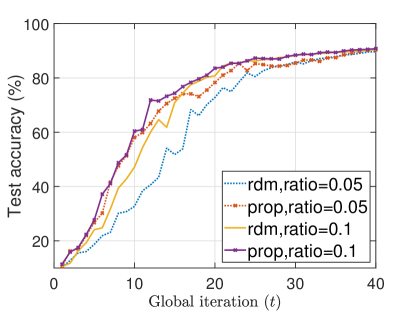
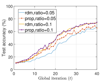
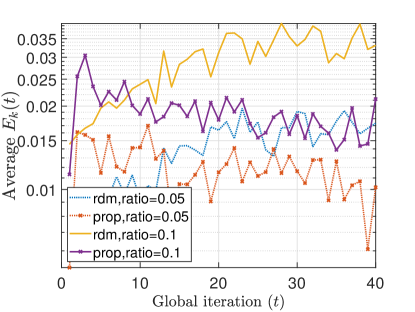
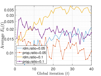
We compare the performance of our proposed design with a baseline method that adopts random scheduling of devices that satisfies the per-round latency requirement. The comparisons of test accuracy are shown in Figs. 1a and 1b, under both i.i.d. and non-i.i.d. data settings. As observed from the simulation results, our method has better test accuracy in the i.i.d. scenario because the proposed scheduling policy prioritizes the devices with higher amounts of fresher data. It also outperforms the alternative method in the non-i.i.d. scenario as the variety of new data is considered in the scheduling criteria, which avoids over-fitting problem by reducing bias in the aggregated model. Moreover, in Figs. 1c and 1d, the comparisons of average per-device energy consumption show that our method consumes less over the learning process. Specifically, we observe and of reduction in power consumption for the case with scheduling ratios and , respectively.
5.2 Effectiveness of the Data Importance Metric
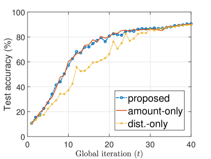
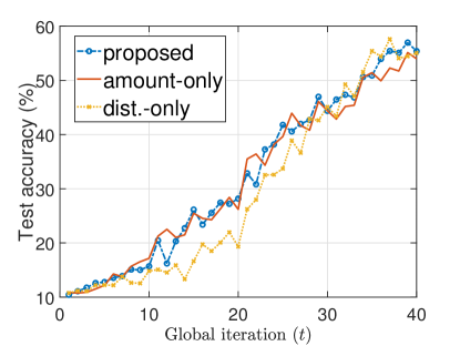
To validate the performance benefits of the proposed data importance metric , we compare (10) with other metrics:
-
•
Amount-only metric, i.e., the first term in (10).
-
•
distribution-only metric, i.e., the second term in (10).
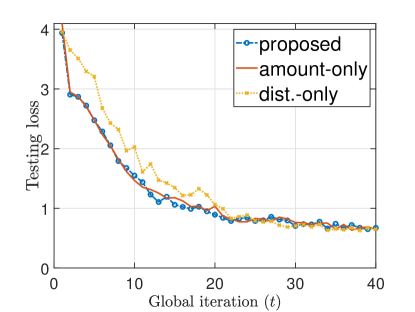
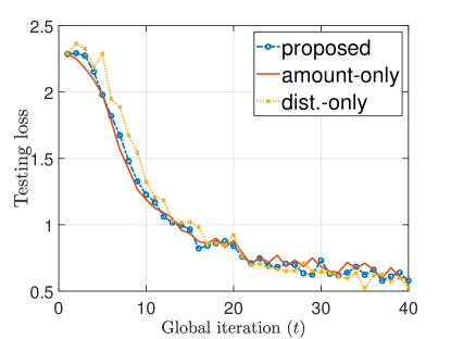
Here, the feature vectors and are computed based on the digit-label distribution of the considered data. The comparison of test accuracy is shown in Fig. 2, which confirms the design aspect of favoring those with higher number of newly arrived data.666In Figs 2, 3, the scaling factor is chosen to be sufficiently large to emphasize more on optimizing the time-average objective. A larger gap of test accuracy between the curves of amount-only and distribution-only methods can be observed at the early iterations, while the distribution-only method achieves a similar and even higher level of test accuracy than the others at the later iterations. The reason behind the huge test accuracy difference is the highly unbalanced timing distribution that data generation at a device follows. In Fig. 3, we have shown the curves of testing loss under different timing distributions. The testing loss difference between the two metrics becomes smaller in the scenario of uniformly distributed timings, since the amount of newly arrived samples per iteration is similar for all the devices. Moreover, the performance gain of distribution-only method at the later stage becomes more clear in Fig. 3b in the considered non-i.i.d. scenario. By combining the benefits of both metrics, the proposed data-importance metric is confirmed to be an effective measure to support an optimal scheduling design.
6 Conclusions
We investigated the problem of device scheduling in a FEEL system with random data generation at edge devices with energy and latency constraints. To deal with the system dynamics in data arrivals and energy consumption, we adopted Lyapunov optimization for designing a dynamic scheduling algorithm that maximizes the long-term data importance from scheduled device sets under constraints on energy consumption and per-round latency. The proposed method showed clear advantages in reducing energy consumption and achieving better learning performance as compared to baseline methods.
References
- [1] E. Rizk, S. Vlaski, and A. H. Sayed, “Federated learning under importance sampling,” IEEE Transactions on Signal Processing, vol. 70, pp. 5381–5396, 2022.
- [2] M. M. Amiri, D. Gündüz, S. R. Kulkarni, and H. Vincent Poor, “Convergence of update aware device scheduling for federated learning at the wireless edge,” IEEE Trans. on Wireless Communications, pp. 1–1, 2021.
- [3] H. Wu and P. Wang, “Node selection toward faster convergence for federated learning on non-iid data,” IEEE Transactions on Network Science and Engineering, vol. 9, no. 5, pp. 3099–3111, 2022.
- [4] C.-H. Hu, Z. Chen, and E. G. Larsson, “Scheduling and aggregation design for asynchronous federated learning over wireless networks,” IEEE Journal on Selected Areas in Communications, pp. 1–1, 2023.
- [5] M. Salehi and E. Hossain, “Federated learning in unreliable and resource-constrained cellular wireless networks,” IEEE Transactions on Communications, vol. 69, no. 8, pp. 5136–5151, 2021.
- [6] F. Malandrino and C. F. Chiasserini, “Federated learning at the network edge: When not all nodes are created equal,” IEEE Communications Magazine, vol. 59, no. 7, pp. 68–73, 2021.
- [7] M. Zhang, G. Zhu, S. Wang, J. Jiang, Q. Liao, C. Zhong, and S. Cui, “Communication-efficient federated edge learning via optimal probabilistic device scheduling,” IEEE Transactions on Wireless Communications, vol. 21, no. 10, pp. 8536–8551, 2022.
- [8] Y. Sun, S. Zhou, and D. Gündüz, “Energy-aware analog aggregation for federated learning with redundant data,” in 2020 IEEE International Conference on Communications (ICC), 2020, pp. 1–7.
- [9] Y. Sun, S. Zhou, Z. Niu, and D. Gündüz, “Dynamic scheduling for over-the-air federated edge learning with energy constraints,” IEEE Journal on Selected Areas in Communications, vol. 40, no. 1, pp. 227–242, 2022.
- [10] J. Xu and H. Wang, “Client selection and bandwidth allocation in wireless federated learning networks: A long-term perspective,” IEEE Transactions on Wireless Communications, vol. 20, no. 2, pp. 1188–1200, 2021.
- [11] K. Guo, Z. Chen, H. H. Yang, and T. Q. S. Quek, “Dynamic scheduling for heterogeneous federated learning in private 5G edge networks,” IEEE Journal of Selected Topics in Signal Processing, vol. 16, no. 1, pp. 26–40, 2022.
- [12] M. Chen, Z. Yang, W. Saad, C. Yin, H. V. Poor, and S. Cui, “A joint learning and communications framework for federated learning over wireless networks,” IEEE Transactions on Wireless Communications, vol. 20, no. 1, pp. 269–283, 2021.
- [13] Y. Li, Y. Cui, and V. Lau, “Optimization-based GenQSGD for federated edge learning,” in 2021 IEEE Global Communications Conference (GLOBECOM), 2021, pp. 1–6.
- [14] A. Albaseer, M. Abdallah, A. Al-Fuqaha, and A. Erbad, “Fine-grained data selection for improved energy efficiency of federated edge learning,” IEEE Transactions on Network Science and Engineering, vol. 9, no. 5, pp. 3258–3271, 2022.
- [15] B. Luo, X. Li, S. Wang, J. Huang, and L. Tassiulas, “Cost-effective federated learning in mobile edge networks,” IEEE Journal on Selected Areas in Communications, vol. 39, no. 12, pp. 3606–3621, 2021.
- [16] S. Wan, J. Lu, P. Fan, Y. Shao, C. Peng, and K. B. Letaief, “Convergence analysis and system design for federated learning over wireless networks,” IEEE Journal on Selected Areas in Communications, vol. 39, no. 12, pp. 3622–3639, 2021.
- [17] J. Zheng, K. Li, E. Tovar, and M. Guizani, “Federated learning for energy-balanced client selection in mobile edge computing,” in 2021 International Wireless Communications and Mobile Computing (IWCMC), 2021, pp. 1942–1947.
- [18] Y. Ji, Z. Kou, X. Zhong, H. Li, F. Yang, and S. Zhang, “Client selection and bandwidth allocation for federated learning: An online optimization perspective,” in 2022 IEEE Global Communications Conference, 2022, pp. 5075–5080.
- [19] L. Yu, R. Albelaihi, X. Sun, N. Ansari, and M. Devetsikiotis, “Jointly optimizing client selection and resource management in wireless federated learning for Internet of Things,” IEEE Internet of Things Journal, vol. 9, no. 6, pp. 4385–4395, 2022.
- [20] Y. Chen, Y. Ning, M. Slawski, and H. Rangwala, “Asynchronous online federated learning for edge devices with non-iid data,” in 2020 IEEE International Conference on Big Data (Big Data). IEEE, 2020, pp. 15–24.
- [21] G. Damaskinos, R. Guerraoui, A.-M. Kermarrec, V. Nitu, R. Patra, and F. Taiani, “Fleet: Online federated learning via staleness awareness and performance prediction,” in Proceedings of the 21st International Middleware Conference, 2020, pp. 163–177.
- [22] A. Mitra, H. Hassani, and G. J. Pappas, “Online federated learning,” in 2021 60th IEEE Conference on Decision and Control (CDC), 2021, pp. 4083–4090.
- [23] E. G. Larsson and O. Gustafsson, “The impact of dynamic voltage and frequency scaling on multicore DSP algorithm design [Exploratory DSP],” IEEE Signal Processing Magazine, vol. 28, no. 3, pp. 127–144, 2011.
- [24] M. J. Neely, “Stochastic network optimization with application to communication and queueing systems,” Synthesis Lectures on Communication Networks, vol. 3, no. 1, pp. 1–211, 2010.
- [25] Y. LeCun and C. Cortes, “MNIST handwritten digit database,” 2010. [Online]. Available: http://yann.lecun.com/exdb/mnist/