Chronosymbolic Learning:
Efficient CHC Solving with
Symbolic Reasoning and Inductive Learning

Abstract

Solving Constrained Horn Clauses (CHCs) is a fundamental challenge behind a wide range of verification and analysis tasks. To improve CHC solving without painstaking manual efforts of creating and tuning various heuristics, data-driven approaches show great promise. However, a large performance gap exists between data-driven CHC solvers and symbolic reasoning-based solvers. In this work, we develop a simple but effective framework, “Chronosymbolic Learning”, which unifies symbolic information and numerical data to solve a CHC system efficiently. We also present a simple instance of Chronosymbolic Learning with a data-driven learner and a BMC-styled reasoner. Despite its great simplicity, experimental results show the efficacy and robustness of our tool. It outperforms state-of-the-art CHC solvers on a test suite of 288 benchmarks, including many instances with non-linear integer arithmetics.

I Introduction

Constrained Horn Clauses (CHCs), a fragment of First Order Logic (FOL), naturally capture the discovery and verification of inductive invariants [2]. CHCs have been widely used in software verification frameworks including C/C++, Java, Rust, Solidity, and Android verification frameworks [3, 4, 5], modular verification of distributed and parameterized systems [6, 7], type inference [8], and many others [9]. Given the importance of these applications, building an efficient CHC solver is of great significance. Remarkable progress has been made in recent years, and existing approaches primarily fall into two categories: symbolic-reasoning-based approaches and data-driven induction-based approaches. The former focuses on designing novel symbolic reasoning techniques, such as abstraction refinement [10], interpolation [11], property-directed reachability [12, 13], model-based projections [14], and other techniques. While the latter focuses on reducing CHC solving into a machine learning problem and then applying proper machine learning models, such as Boolean functions [15], decision trees (DTs) [16], support vector machines (SVMs) [17], and deep learning models [18].

The undecidable nature of CHC solving suggests that special adjustments or new designs are necessary for specific instances, demanding non-trivial effort and expertise. On the other hand, although data-driven approaches show great promise towards improving CHC solving without the painstaking manual effort of creating and tuning various heuristics, data-driven CHC solvers still fall way behind symbolic reasoning-based CHC solvers [19]. Fig. 1 illustrates some important differences between these two categories in the view of learning from positive and negative data points. Symbolic-reasoning-based approaches usually maintain two zones, which are approximations of safe and unsafe “states” of a system represented by given CHCs and carefully updated with soundness guarantees. Data-driven approaches abstract given symbolic constraints away by sampling positive and negative data points. The sampling process usually requires some form of evaluation of the given constraints, thus, sampled data points are the outcome of complicated interactions among multiple constraints, making data-driven approaches excel at capturing useful global properties. However, as illustrated by the dashed grey line in Fig. 1, the main disadvantage of data-driven approaches is that the classifier learned from samples may miss part of safe regions that could be easily found by symbolic reasoning. In contrast, symbolic-reasoning approaches are good at precisely analyzing local constraints, which enables superior performance but may also make the solving process stuck in a local region. In addition, in many cases, symbolic reasoning is far more expensive than sampling data points. However, such approaches struggle to identify the important patterns from data samples, making them inflexible in dealing with these problems.

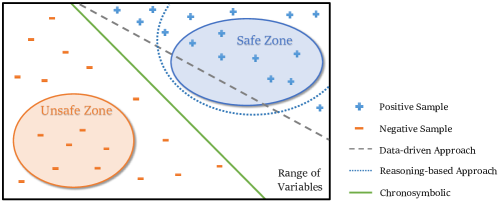
Figure 1: Overview of different approaches through the lens of learning from positive samples and negative samples.

We propose a simple but effective framework, Chronosymbolic Learning, and as the name suggests, our goal is to solve CHCs with both numerical (“no.”) data samples and symbolic information in a synchronous and synergistic manner. Like data-driven approaches, Chronosymbolic Learning uses machine learning to get classifiers from sampled data points. Then, instead of directly using learned classifiers as candidate solutions, we further augment them with symbolic information. The symbolic information can be viewed as a region of data points concisely represented in a symbolic manner. Conversely, learned classifiers can be viewed as a symbolic representation of a generalized region. Instead of just combining these two mechanically or parallelly, our method makes the reasoner and learner mutually benefit from each other, as illustrated by the green line of Fig. 1.

Main Contributions: Our contribution is mainly three-fold. First and foremost, we propose a new framework, Chronosymbolic Learning, which can leverage both symbolic information and numerical data points for CHC solving. It also introduces the fundamentals of seamlessly synergizing data learning power with automated reasoning power, and provides a paradigm for future works that could incorporate up-to-date ML approaches. Secondly, we provide a simple yet effective instance of Chronosymbolic Learning, which is composed of a data-driven learner interacting with a BMC-styled reasoner, and a verification oracle as a teacher. Lastly, the experiment results demonstrate the effectiveness and robustness of our tool. It outperforms several state-of-the-art CHC solvers on a dataset of 288 benchmarks, including many instances with non-linear integer arithmetic.

II Preliminaries

II-A Constrained Horn Clauses

We discuss standard First Order Logic (FOL) formula modulo theory $\mathcal{T}$, with a signature $\Sigma$ composed by constant symbols $\mathcal{A}$ (e.g., True $\top$ and False $\bot$ ), function symbols $\mathcal{F}$ (e.g., +, -, mod) and predicate symbols $\mathcal{P}$. A Constrained Horn Clause (CHC) $\mathcal{C}$ is a FOL formula modulo theory $\mathcal{T}$ in the following form:

$$\forall\mathcal{X}\cdot\phi\land p_{1}(T_{1})\land\cdots\land p_{k}(T_{k})\rightarrow h(T),\ k\geq 0,$$ (1)

where $\mathcal{X}$ stands for all variables in $T_{i}$ and $T$, $\phi$ represents a fixed constraint over $\mathcal{F};\mathcal{A}\text{ and }\mathcal{X}$ w.r.t. some background theory $\mathcal{T}$; $p_{i},h$ are predicate symbols, and $p_{i}(T_{i})=p_{i}(t_{i,1},\cdots,t_{i,n})$ is an application of n-ary predicate symbol $p_{i}$ with first-order terms $t_{i,j}$ built from $\mathcal{F},\mathcal{A}\text{ and }\mathcal{X}$; $h(T)$ could be either $\mathcal{P}$-free (i.e., no predicate symbol appears in $h$) or akin to the definition of $p_{i}(T_{i})$.

As an example, in this work, we explain our framework using the background theory of Integer Arithmetic (IA) if it is not specified. For simplification, in our work, the quantifier $\forall$ is omitted when the context is clear; and all terms $t_{i,j}$ can be substituted by single variables (e.g., $t_{1,1}=x$, $t_{1,2}=y$).

The structure of a CHC can be seen as splitting by the implication symbol. The left hand side $\phi\wedge p_{1}(T_{1})\wedge\cdots\wedge p_{k}(T_{k})$ is called body and the right hand side $h(T)$ is call head. If the body of a CHC contains zero or one predicate symbol, the CHC is called linear. Otherwise, it is called non-linear.

Example 1.

A simple CHC system $\mathcal{H}_{0}$ consists of a fact $\mathcal{C}_{0}$, a non-fact rule $\mathcal{C}_{1}$ and a query $\mathcal{C}_{2}$ is as follows:

$$\quad\mathcal{C}_{0}: \ \neg(a\leq 0)\ \land\ b\leq a\ \land\ c=0\ \land\ e=0\ \land\ d=0$$

$$\rightarrow inv(a,b,c,d,e)$$

$$\mathcal{C}_{1}: \ c_{1}=1+c\land d_{1}=d+a\land e_{1}=e+b\land inv(a,b,c,d,e)$$

$$\rightarrow inv(a,b,c_{1},d_{1},e_{1})$$

$$\mathcal{C}_{2}: \ \neg(e\geq a\cdot c)\ \land\ inv(a,b,c,d,e)\rightarrow\bot$$

In most cases, the terminology “CHC solving” refers to solving the satisfiability (SAT) problem for a CHC system $\mathcal{H}$ that is a set of CHCs containing at least a query and a rule. A query $\mathcal{C}_{q}$ refers to a CHC that has a $\mathcal{P}$-free head, otherwise, it is called a rule $\mathcal{C}_{r}$. Particularly, a fact $\mathcal{C}_{f}$ refers to a rule that has a $\mathcal{P}$-free body. For example, in Example 1, $\mathcal{C}_{0}$ is a fact and a rule, $\mathcal{C}_{1}$ is a rule, and $\mathcal{C}_{2}$ is a query. We define the clauses that both body and head are $\mathcal{P}$-free as trivial clauses, because they can be simply reduced to $\top$ or $\bot$. Then, we formally define the satisfiability of a CHC system $\mathcal{H}$:

Definition 1 (Satisfiability of a CHC).

A CHC $\mathcal{C}:\phi\land p_{1}(T_{1})\land\cdots\land p_{k}(T_{k})\rightarrow h(T)$ is satisfiable (SAT) iff there exists an interpretation of predicates $\mathcal{I}$, the constraint $\mathcal{I}\left[\mathcal{C}\right]:\phi\land\mathcal{I}\left[p_{i}\right](T_{1})\land\cdots\land\mathcal{I}\left[p_{k}\right](T_{k})\rightarrow\mathcal{I}\left[h\right](T)$ is SAT. Otherwise, we say $\mathcal{C}$ is unsatisfiable (UNSAT).

Definition 2 (Satisfiability of a CHC system).

A CHC system $\mathcal{H}$ is satisfiable (SAT) iff there exists an interpretation of predicates $\mathcal{I}^{*}$, $\forall\mathcal{C}\in\mathcal{H}$, $\mathcal{I}^{*}\left[\mathcal{C}\right]$ is SAT. Otherwise, we say $\mathcal{H}$ is unsatisfiable (UNSAT).

Definition 3 (Solution of a CHC system).

If a CHC system $\mathcal{H}$ is SAT, the solution of $\mathcal{H}$ is the corresponding interpretation $\mathcal{I}^{*}$, and $\mathcal{I}^{*}[p]$ is called a solution interpretation of the predicate $p$. If a CHC system $\mathcal{H}$ is UNSAT, the solution of $\mathcal{H}$ is a refutation proof that there is no such interpretation [20].

The refutation proof can be seen as a specific value assignment for all the variables in $\mathcal{H}$ that can refute all the CHCs in $\mathcal{H}$. Hence, the problem discussed in this work is to find a solution to a given CHC system.

II-B Hypothesis Learning as a Classification Problem

To leverage the information provided by the data samples, we reduce the hypothesis learning problem to a classification problem. Now, for the convenience of our discussion, we formally define what a hypothesis is:

Definition 4.

Hypothesis refers to an interpretation $\tilde{\mathcal{I}}$ that is a possible solution of a CHC system $\mathcal{H}$. The hypothesis for a specific predicate $p$ is denoted as $\tilde{\mathcal{I}}\left[p\right]$.

To figure out an interpretation $\tilde{\mathcal{I}}\left[p\right]$ for a specific predicate $p$, we introduce a lightweight machine learning toolchain that combines DT learning with the results of SVMs [17].

In this data-driven pipeline, the positive and negative samples are first classified by the SVMs multiple times until all the samples are properly classified. The resulting hyperplanes of SVMs, $f(\boldsymbol{x})=w^{T}\boldsymbol{x}_{i}+b$, are passed to the DT as attributes. The DT then selects an attribute $f(\boldsymbol{x}_{0})$ and a corresponding threshold $c$ in the form of $f(\boldsymbol{x}_{0})\leq c$ to form a new node in the way of maximizing the information gain $\gamma$ in Appendix, Equation 9. Adjusting the threshold $c$ and pruning the over-complicated combination of attributes makes the toolchain more generalizable and lowers the risk of the over-fitting issue. In this way, a DT is formed step-by-step, which separates all samples into positive and negative categories. The learned formula $\mathcal{L}_{p}$ converted by the DT can be arbitrary linear inequalities and their combinations in disjunctive normal form (DNF). It is also called a partition in our framework, which is a valid hypothesis for $p$ and a potential part of the solution of the CHC system.

III Chronosymbolic Learning

As shown in Fig. 1, pure data-driven and reasoning-based approaches are limited in different ways. The former is completely agnostic to the inherent symbolic information of the given CHC system, and can only draw hypotheses by guessing from data samples. The latter has difficulty inducing global patterns of correct interpretations of a predicate, and are weak in incorporating the data samples into their reasoning process.

To address the limitations, we propose Chronosymbolic Learning, a modular framework that combines the merits of both approaches and makes the best use of symbolic information and numerical data simultaneously.

Figure 2: The architecture of Chronosymbolic Learning.

III-A Architecture of Chronosymbolic Learning

The architecture of our instance of Chronosymbolic Learning is shown in Fig. 2. Chronosymbolic Learning is the extension of the paradigm of “teacher and learner” [21], which can find a solution to a given CHC system by guessing and checking [22]. In this paradigm, the teacher and learner talk to each other in each iteration. For each iteration, the learner makes a hypothesis (see Definition 4) of an interpretation called partition, and the teacher verifies the hypothesis and gives instant feedback on whether it is correct; if it is incorrect, the teacher returns a counterexample (see Definition 9) on why it is incorrect.

In addition to this paradigm, in Chronosymbolic Learning, the learning procedure is enhanced by a reasoner. The reasoner keeps track of a safe zone and an unsafe zone, which are symbolic representations of positive and negative samples respectively. There are mainly three benefits of keeping such zones: 1) they can be incorporated into the hypothesis proposed by the learner to enhance the hypothesis; 2) they provide the learner with additional samples; 3) they greatly simplify the UNSAT checking of the CHC system. We will provide an instance of Chronosymbolic Learning, and elaborate on how modules of our instance work and how they communicate with each other as in Fig. 2. The learner we propose in Section IV-A and reasoner in Section IV-B can be replaced by any other algorithms that can produce partitions and zones.

III-B Samples and Zones

To formally define Chronosymbolic Learning, we first introduce the concepts of positive, negative, and implication samples. We will shed light on obtaining the samples in Section IV-A.

Definition 5 (Positive Sample).

A data point $s^{+}$ is a positive sample of predicate $p$ in $\mathcal{H}$ iff for each solution interpretation $\mathcal{I}^{*}$ of $\mathcal{H}$, we have $\mathcal{I}^{*}\left[p\right](s^{+})=\top$.

Definition 6 (Negative Sample).

A data point $s^{-}$ is a negative sample of predicate $p$ in $\mathcal{H}$ iff for each solution interpretation $\mathcal{I}^{*}$ of $\mathcal{H}$, we have $\mathcal{I}^{*}\left[p\right](s^{-})=\bot$.

Definition 7 (Implication Sample).

An implication sample $s^{\rightarrow}$ of body predicates $(p_{1},...,p_{n})$ and head predicate $h$ in $\mathcal{H}$ is a $(n+1)$-tuple of data points $\left(s^{\rightarrow}_{1},\cdots,s^{\rightarrow}_{n},s^{\rightarrow}_{h}\right)$ such that for each solution interpretation $\mathcal{I}^{*}$ of $\mathcal{H}$, we have $\mathcal{I}^{*}\left[p_{1}\right]\left(s^{\rightarrow}_{1}\right)\land\cdots\land\mathcal{I}^{*}\left[p_{n}\right]\left(s^{\rightarrow}_{n}\right)\rightarrow\mathcal{I}^{*}\left[h\right]\left(s^{\rightarrow}_{h}\right)$.

Example 2.

In $\mathcal{H}_{0}$ of Example 1, for predicate $inv$, $s^{+}=(1,1,0,0,0)$ is a positive sample, since $s^{+}[\mathcal{C}_{0}]:\top\rightarrow inv(1,1,0,0,0)$. $s^{-}=(2,1,5,0,5)$ is a negative sample, since $s^{-}[\mathcal{C}_{2}]:inv(2,1,5,0,5)\rightarrow\bot$. $s^{\rightarrow}=(1,1,0,0,0)\rightarrow(1,1,1,1,1)$ is a implication sample, since $s^{\rightarrow}[\mathcal{C}_{1}]:inv(1,1,0,0,0)\rightarrow inv(1,1,1,1,1)$.

With the definition of samples, we now formally define safe and unsafe zones. The word “safe” and “unsafe” comes from “safe and unsafe program states” in program verification, which means states that can be reached and states that conflict with the assertion (the condition to be verified).

Definition 8 (Safe Zone and Unsafe Zone).

The safe zone of the predicate $p$, $\mathcal{S}_{p}$, is a set of positive samples. The unsafe zone of the predicate $p$, $\mathcal{U}_{p}$, is a set of negative samples.

The zones can be represented as symbolic expressions, such as inequalities and equations. They can contain zero samples, or contain a finite or infinite number of samples. Notably, a positive sample can also be seen as a safe zone, and a negative sample can be seen as an unsafe zone.

Example 3.

In $\mathcal{H}_{0}$ in Example 1, one safe zone for predicate $inv(v_{0},v_{1},v_{2},v_{3},v_{4})$ is $\mathcal{S}_{inv}=\neg(v_{0}\leq 0)\ \land\ v_{1}\leq v_{0}\ \land\ v_{2}=0\ \land\ v_{3}=0\ \land\ v_{4}=0$, since $s^{+}\in\mathcal{S}_{inv}$ satisfies $s^{+}[\mathcal{C}_{0}]:\top\rightarrow inv(s^{+})$. One unsafe zone for predicate $inv$ is $\mathcal{U}_{inv}=\neg(v_{4}\geq v_{0}v_{2})$, since $s^{-}\in\mathcal{U}_{inv}$ satisfies $s^{-}[\mathcal{C}_{2}]:inv(s^{-})\rightarrow\bot$.

III-C Incorporate Zones within Learning Iterations

TABLE I: Several candidates of hypotheses.

Methods	Hypothesis
BMC-styled	$$\tilde{\mathcal{I}}_{s}\left[p_{i}\right]=\mathcal{S}_{p_{i}}\qquad$$ (2)
LinearArbitrary-styled	$$\tilde{\mathcal{I}}_{l}\left[p_{i}\right]=\mathcal{L}_{p_{i}}\qquad$$ (3)
Chronosymbolic without safe zones	$$\tilde{\mathcal{I}}_{lu}\left[p_{i}\right]=\mathcal{L}_{p_{i}}\land\neg\ \mathcal{U}_{p_{i}}\qquad$$ (4)
Chronosymbolic without unsafe zones	$$\tilde{\mathcal{I}}_{sl}\left[p_{i}\right]=\mathcal{S}_{p_{i}}\lor\mathcal{L}_{p_{i}}\qquad$$ (5)
Chronosymbolic	$$\tilde{\mathcal{I}}_{slu}\left[p_{i}\right]=\mathcal{S}_{p_{i}}\lor\left(\mathcal{L}_{p_{i}}\land\neg\ \mathcal{U}_{p_{i}}\right)\quad$$ (6)

Chronosymbolic Learning is a framework that incorporates zones within the learning iterations. A Chronosymbolic Learner proposes the hypothesis $\tilde{\mathcal{I}}\left[p_{i}\right]$ considering currently reasoned safe zones $\mathcal{S}_{p_{i}}$, unsafe zones $\mathcal{U}_{p_{i}}$ from the reasoner with the inductive results (partitions) of the learner $\mathcal{L}_{p_{i}}$.

Several promising candidates of the hypothesis $\tilde{\mathcal{I}}\left[p_{i}\right]$ that can be made by Chronosymbolic Learner are listed in Table I. We have the following lemma:

Lemma 1.

$\tilde{\mathcal{I}}_{slu}\succeq\{\tilde{\mathcal{I}}_{sl},\tilde{\mathcal{I}}_{lu}\}\succeq\tilde{\mathcal{I}}_{l}$, where $A\succeq B$ denotes that A is a solution interpretation of the CHC system $\mathcal{H}$ whenever B is a solution interpretation.

Intuitively, Lemma 1 shows the order of the feasibility of becoming a solution of predicate $p_{i}$. We give a proof sketch for $\tilde{\mathcal{I}}_{sl}\succeq\tilde{\mathcal{I}}_{l}$ and proofs for others are similar. Assume $\tilde{\mathcal{I}}_{l}\left[p_{i}\right]=\mathcal{L}_{p_{i}}$ is a solution interpretation of $\mathcal{H}$, and then by Definition 5, we have for each positive sample $s^{+}$, $\tilde{\mathcal{I}}_{l}\left[p_{i}\right](s^{+})=\top$, i.e., $s^{+}\in\tilde{\mathcal{I}}_{l}\left[p_{i}\right]$. According to Definition 8, the safe zone $\mathcal{S}_{p_{i}}$ is a set of positive samples, and we have $\mathcal{S}_{p_{i}}\subset\tilde{\mathcal{I}}_{l}\left[p_{i}\right]$. We now have $\tilde{\mathcal{I}}_{sl}\left[p_{i}\right]=\mathcal{S}_{p_{i}}\land\tilde{\mathcal{I}}_{l}\left[p_{i}\right]=\tilde{\mathcal{I}}_{l}\left[p_{i}\right]$ and $\tilde{\mathcal{I}}_{sl}\left[p_{i}\right]$ is also a solution interpretation. Thus, we can conclude $\tilde{\mathcal{I}}_{sl}\succeq\tilde{\mathcal{I}}_{l}$.∎

In practice, if we always use one above-mentioned hypothesis pattern, Equation 6 achieves the best result, as it generally carries more information summarized by both the learner and the reasoner. However, it is not always the case for a single instance, since the zones may carry “distractive” information. To address this issue, we can manually apply adequate strategies on each instance, or use a scheduler to alternate those candidate hypotheses over time. In the experiment, we will show the performance gain of applying different strategies.

III-D Overall Algorithm

Algorithm 1 Chronosymbolic Learning $\left(\mathcal{H}\right)$

0:  A CHC system $\mathcal{H}=\{\mathcal{C}_{0},\cdots,\mathcal{C}_{n}\}$

1:  $\bullet$ Initialize safe and unsafe zones   $\forall\ p_{i},\ (\mathcal{S}_{p_{i}},\mathcal{U}_{p_{i}})$ $\leftarrow$ $(\bot,\bot)$

2:  $\bullet$ Initialize the hypotheses  $\forall\ p_{i},\ \tilde{\mathcal{I}}_{p_{i}}$ $\leftarrow$ $\top$

3:  $\bullet$ Initialize UNSAT flag   $is\_unsat$ $\leftarrow(\top,\bot)$

4:  $\bullet$ Initialize the dataset      $\mathcal{D}\leftarrow\varnothing$

5:  while not $is\_unsat$ and $\exists\ \mathcal{C}_{i},$ not SMTCheck($\tilde{\mathcal{I}}\left[\mathcal{C}_{i}\right]$) do

6:     $\circ$ Reasoning and UNSAT checking   $\ (\mathcal{S}$, $\mathcal{U}$, $is\_unsat)$ $\leftarrow$ reason($\mathcal{H}$, $\mathcal{S}$, $\mathcal{U}$)

7:     $\circ$ Sample from zones and add to $\mathcal{D}$   $\mathcal{D}\leftarrow$ sampling($\mathcal{S}$, $\mathcal{U},\mathcal{D}$)

8:     for each $\mathcal{C}_{i}\in\mathcal{H}$ do

9:        while not SMTCheck($\tilde{\mathcal{I}}\left[\mathcal{C}_{i}\right]$) do

10:           $\bullet$ Find counterexample(s)   $c\leftarrow$ SMTModel($\tilde{\mathcal{I}}\left[\mathcal{C}_{i}\right]$)

11:           $\bullet$ Convert counterexample(s) to samples   $s\leftarrow$ converting(c)

12:           $\bullet$ UNSAT checking   $is\_unsat$ $\leftarrow$ checkUNSAT($\mathcal{D}$, s)

13:           $\bullet$ Add samples to $\mathcal{D}$    $\mathcal{D}\leftarrow s$, if not $is\_unsat$

14:           $\bullet$ Learn a partition   $\mathcal{L}\leftarrow$ learn($\mathcal{D}$)

15:           $\bullet$ Update the hypothesis   $\tilde{\mathcal{I}}\leftarrow$ makeHypothesis($\mathcal{S},\mathcal{U},\mathcal{L}$)

16:        end while

17:     end for

18:  end while

18:  A solution ($is\_unsat,\ \tilde{\mathcal{I}}$) for the CHC system $\mathcal{H}$

The overall algorithm is described in Algorithm 1, where the solid bullet points mean “mandatory” and the unfilled bullet points mean “optional”, indicating that it is unnecessary to execute in every iteration.

The algorithm takes a CHC system $\mathcal{H}$ as input and outputs a solution of it. We first initialize the zones, hypotheses, UNSAT flag, and dataset properly in lines 1-4. The outer while loop from lines 5 to 18 checks if a solution of $\mathcal{H}$ is reached, and if not, it starts a new epoch and continues solving. In line 5, SMTCheck($\tilde{\mathcal{I}}\left[\mathcal{C}_{i}\right]$) calls the backend SMT solver to check the satisfiability of a CHC $\mathcal{C}_{i}$ under current hypothesis interpretation $\tilde{\mathcal{I}}$. In line 6, the reasoner refines the zones and checks if the zones overlap (see Section IV-B). Line 7 is the sampling procedure described in Section VIII-C1.

The for loop from line 8 to 17 iteratively finds an UNSAT CHC and updates the hypothesis until it is SAT. In the inner while loop in lines 10-13, we find one or a batch of counterexamples, convert them into samples, and add them to the dataset after the UNSAT checking passes. SMTModel($\tilde{\mathcal{I}}\left[\mathcal{C}_{i}\right]$) in line 10 calls the backend SMT solver to return a counterexample that explains why the current hypothesis is invalid. Once the dataset has been updated, in lines 14-15, the learner induces a new partition, and we can then update the Chronosymbolic hypothesis using some ways to combine the information of the zones and the partition, which is described in I. The new hypothesis is guaranteed to make progress because it incorporates the new information collected in this iteration.

IV Design of Learner and Reasoner

IV-A Learner: Data-Driven CHC Solving

The learner module in our tool leverages an induction-based and CEGAR-inspired [10] CHC solving scheme. It has two sub-modules: the dataset and the machine learning toolchain. The dataset stores the positive and negative samples and the corresponding predicates for inductive learning. The machine learning toolchain (an example is introduced in Section II-B) takes the samples in the dataset as input and outputs a partition that can correctly classify all these samples.

The samples are converted from counterexamples. As shown in Fig. 2, the counterexample provided by the teacher is essential in the learning loop, since it offers the learner information about why the current hypothesis is incorrect and how to improve it. Here we formally define the term “counterexample”.

Definition 9 (Counterexample).

A counterexample $c=\left((c_{p_{1}},\cdots,c_{p_{k}}),c_{h}\right)$ for an interpreted CHC $\mathcal{I}\left[\mathcal{C}\right]:\forall\mathcal{X}\cdot\phi\land\mathcal{I}\left[p_{1}\right](T_{1})\land\cdots\land\mathcal{I}\left[p_{k}\right](T_{k})\rightarrow\mathcal{I}\left[h\right](T),\ k\geq 0$ is a value assignment for variables $\mathcal{X}$, such that under the interpretation $\mathcal{I}$ and such an assignment, $\mathcal{I}\left[\mathcal{C}\right]$ is UNSAT.

Example 4.

In $\mathcal{H}_{0}$ in Example 1, given that the current hypothesis of predicate $inv(v_{0},v_{1},v_{2},v_{3},v_{4})$ is $\tilde{\mathcal{I}}\left[inv\right]=v_{3}\leq 1$, a counterexample for $\mathcal{C}_{1}$ could be $c=(((2,0,0,0,0)),(2,0,1,2,0))$, as it makes $\tilde{\mathcal{I}}[\mathcal{C}_{1}]:\top\rightarrow\bot$.

The counterexamples can be converted into positive, negative, or implication samples through the converting procedure in Fig. 2 and Algorithm 1. The counterexamples carry information that makes the hypothesis more accurate. We introduce a three-way converting scheme that can convert counterexamples to positive, negative, and implication samples according to the type of the CHC. This could also be seen as sampling the CHC system in three directions: forward, backward, and midway.

Lemma 2 (Sample Converting).

The counterexample of a fact can provide a positive sample for the head predicate. If a query is linear, the counterexample of the query can provide a negative sample for the body predicate. The counterexample of a rule can provide an implication sample from the body predicate(s) to the head predicates if the rule is not a fact.

To make implication samples easier to handle, we define the term tentative sample as follows.

Definition 10 (Tentative Sample).

A tentative positive (negative) sample $\tilde{s}^{+}$ $(\tilde{s}^{-})$ of predicate $p$ is a data point such that, after using some generalization methods, the learner tentatively deems it to be a positive (negative) sample, but the sample may not meet the requirements in Definition 5 (6).

Lemma 3 (Implication Sample Converting).

For an implication sample $s^{\rightarrow}$, if the $n$ samples in $(s^{\rightarrow}_{1},\cdots,s^{\rightarrow}_{n})$ are all positive samples (or in the safe zone), then $s^{\rightarrow}_{h}$ is a positive sample. If samples in $s^{\rightarrow}_{h}$ is a negative sample (or in the unsafe zone), and $n=1$, the sample $s^{\rightarrow}_{1}$ is a negative sample. Otherwise, the sample can only be converted into tentative positive or negative samples, whose categories make the logical implication hold.

Empirically, converting all tentative samples into negative tentative samples is a decent design choice. As these samples are not guaranteed to be positive or negative, they should be cleared periodically to prevent keeping the “wrong guess” in a specific tentative category forever. After such conversion, only positive and negative samples exist from the learner’s view. It is natural to leverage off-the-shelf machine learning tools on binary classification, e.g., the toolchain in Section II-B.

IV-B Reasoner: Zones Discovery

We adopt a simple BMC-styled logical reasoning procedure for inferring safe and unsafe zones in our tool. It serves as the reasoner of our instance of Chronosymbolic Learning. The reasoner is not expected to reason about a complete hypothesis, but to provide a “partial solution” in the format of safe and unsafe zones, which collaborates well with the learner. In our tool, the reasoner initializes the zones, expands the zones through image (or pre-image) computation, and does UNSAT checking. The zones summarize the information within a bounded number of transitions.

IV-C Implementation Details

As for the learner, the DT and SVM implementation is almost the same as [17]. For DT, the algorithm we used is C5.0 [23]. We add some default features that can make the tool more efficient. Some of those features provide common patterns in inductive invariants, such as the octagon abstract domain [24] ($\pm v1\pm v2\geq c$). The other features provide extensions for some non-linear operators, e.g., mod. We implement an auto-find feature that finds the “mod $k$” patterns in the CHC system automatically. It resembles the idea of some synthesis-based methods like FreqHorn [25], which takes often-appearing patterns in the CHC system as a part of the grammar. For more detail on the machine learning toolchain, please refer to Section II-B and [17]. For the dataset described in Section IV-A, we provide two ways of implementation. One way is to collect all data samples until the current iteration and send all samples to the learner. This approach is accurate and guaranteed to make progress, but it is increasingly burdensome for the learner to induce a partition. Another way is to keep recent $a$ positive and $b$ negative samples in a queue. This makes the learner more efficient but less precise and has no guarantee of making progress. Empirically, the two approaches achieve nearly the same performance.

As for the reasoner, our implementation is a lightweight one and is designed to assist the learner in making better hypotheses. To keep the zones simple, our implementation only initializes and expands at the beginning of the learning iterations. The simple zones bring less burden to the backend SMT solver, making the guess-and-check procedure smooth. The expansion of zones is also controlled by several hyperparameters to keep the zones lightweight, and some examples are shown in Section V-A.

To handle CHC systems in different styles and formats, we preprocess the input CHC system in these aspects: 1) rewrite the terms in predicates to ensure that the predicates are only parameterized by distinctive variables (such as $p(v_{0},v_{1},v_{2})$); 2) clear and propagate predicates that are $\top$ or $\bot$; 3) simplify the inner structure of each CHC if possible.

V Experiments

V-A Experimental Settings

Benchmarks

Our benchmarking dataset is a collection of widely-used arithmetic CHC benchmarks from some related works [26, 25, 16] and SV-COMP, collected by FreqHorn [25]. It is a suite of $288$ instances in total, in which $235$ are safe ones, and $53$ are unsafe ones. The instances are lightweight, arithmetic CHC benchmarks, but many of them require non-trivial effort to reason about the correct interpretation due to the complexity of the arithmetic. Most instances are under linear arithmetic, and a few require the ability to deal with simple non-linear arithmetic. We also discuss some results on CHC-COMP-22, LIA track. See Appendix for details.

Implementation Details

Our implementation of Chronosymbolic Learning is built in Python 3.10. The backend SMT solver we use is Microsoft Z3 [27] 4.8.11.0. Our tool supports the SMT-LIB2 [28] format and the Datalog (rule-query) format. See Appendix for details.

Hyperparameters

For the learner, in SVM, the $C$ parameter is set to $1$. The upper limit of the coefficients in the hyperplanes is set to $10$. For the reasoner, as for zone expansion strategy, to avoid the zones being over-complicated and slowing down the backend solver, if the length of the body constraint is larger than 500, the CHC is skipped when expanding. If the length of a zone is larger than 1500, the expansion of this zone is stopped. If the expansion of a zone introduces a quantifier that is not able to eliminate, the expansion procedure of this zone would also be stopped.

Experiment Setup

We set the timeout of solving a CHC system instance as $360$ seconds for all tools. Since there is some randomness in the tools, we repeat three times for each experiment and report the best result.

V-B Baselines

State-of-the-art CHC solvers can be classified into three categories: reasoning-based, synthesis-based, and induction-based solvers (see Section VI). We compare our method against the representatives of the three types of solvers as follows:

LinearArbitrary

LinearArbitrary [17] is the state-of-the-art induction-based solver that learns inductive invariants from the samples derived by counterexample using SVM and DT. We use the default hyperparameters in the paper and their open-source code. The implementation only supports C programs and Datalog (rule-query) format of CHC instances.

FreqHorn

FreqHorn [25] is a representative of synthesis-based solvers that synthesizes the invariant using a frequency distribution of patterns. It cannot determine the CHC system as UNSAT, and it resorts to external tools to do that. In the experiment, we follow the default settings in [25].

Spacer and GSpacer

Spacer [14] is a powerful SMT-based CHC-solving engine serving as the default CHC engine in Microsoft Z3 [27]. The experiment is conducted under the default settings of Microsoft Z3 4.8.11.0. GSpacer [19] achieves state-of-the-art on many existing CHC benchmarks by extending with some well-designed global guidance heuristics. To achieve the best result, we enable all the heuristics, including the subsume, concretize, and conjecture rules.

V-C Performance Evaluation

The performance comparison with each baseline is shown in Table V. The configuration “Chronosymbolic-single” stands for the best result in a single run of our solver. In this setting, all instances are tested using a fixed set of hyperparameters. “Chronosymbolic-cover” stands for all solved benchmarks covered by 13 runs using different strategies and hyperparameters, which shows the potential capability of our framework if we choose adequate strategies and hyperparameters for each instance. We do not show the timing for this setting because the time to solve a certain benchmark varies among different runs. Fig. 3 shows the runtime comparison.

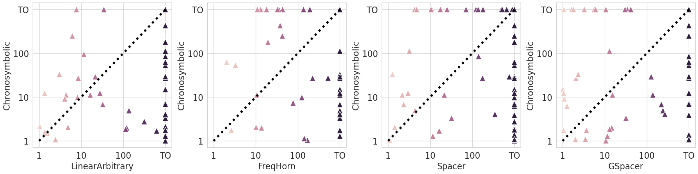
Figure 3: Running time comparison of Chronosymbolic Learning and baselines, where the timeout (TO) is 360 seconds. The points below the diagonal indicate instances on which Chronosymbolic-single outperforms baselines. Here, we only plot non-trivial instances (i.e., solving time takes $\geq 1$ second for both solvers).

TABLE II: Performance evaluation of methods. “#total” stands for the total number of solved instances and “percentage” for the percentage of solved ones among all 288 instances, “#safe” for solved ones among 235 safe instances, “#unsafe” for solved ones among 53 unsafe instances. For timing, “avg-T” is the average time (seconds) consumed on each instance (including timeout or crashed ones), and “avg-T-solved” is the average time (seconds) consumed on each solved instance.

Method	#total	percentage	#safe	#unsafe	avg-T	avg-T-solved
LinearArbitrary	187	64.93%	148	39	135.0	13.48
FreqHorn	191	66.32%	191	0	129.1	11.80
Spacer	184	63.89%	132	52	132.8	15.30
GSpacer	220	76.39%	174	46	83.50	7.83
Chronosymbolic single	237	82.29%	189	48	68.33	7.51
Chronosymbolic cover	255	88.54%	207	48	-	-

The result shows that, even in the Chronosymbolic-single setting, our tool successfully solves $17$ more instances than the best solver among other compared approaches, GSpacer, and generally beats other solvers in terms of speed, even though our tool is implemented in Python. This result shows that our tool performs considerably even without careful tuning for each CHC instance. For the Chronosymbolic-cover setting, the result is more significant than other candidates, which indicates the necessity of finding adequate strategies for different instances. Among other approaches, GSpacer performs the best on solved instances and time consumed, as shown in other literature. Nevertheless, in our experiment, we find that Spacer, GSpacer, and LinearArbitrary fail to solve most instances with non-linear arithmetic. FreqHorn can solve some of them, but fails in all unsafe instances without the resort to external tools. Our approach can also handle some of the non-linear arithmetic benchmarks because our reasoner can provide zones in non-linear arithmetic.

V-D Ablation Study

We further study the effectiveness of the critical parts of our framework: the learner and the reasoner. For the reasoner, we compare the result of not providing safe zones, not providing unsafe zones, and neither. We experiment with taking the learner away as a whole and run our tool with the mere reasoner. While conducting the ablation study, we keep the other settings the same as Chronosymbolic-single.

TABLE III: Ablation study for different configurations of Chronosymbolic Learning.

Configuration	#total	percentage	#safe	#unsafe	avg-T	avg-T
w/o safe zones	228	79.17%	183	45	78.56	9.11
w/o unsafe zones	218	75.69%	173	45	94.75	12.87
w/o both zones	211	73.26%	166	45	93.84	10.09
w/o learner	131	45.49%	96	35	196.3	0.16
Chronosymbolic single	237	82.29%	189	48	68.33	7.51

From Table III, as expected, Chronosymbolic-single comprehensively outperforms all other configurations, which shows that each component of our framework is indispensable. It is also clear that each zone provides useful information to the hypothesis, making the result of Chronosymbolic without both zones worse than without safe and unsafe zones. As mentioned in Section VIII-D2 and Appendix, our reasoner is lightweight and is designed to assist the learner. Thus, the result of not using a learner is the worst, but we can get the result quickly. The result also shows that our learner performs much better than LinearArbitrary, as we have a more comprehensive converting and sampling scheme.

Another experiment shows that if we run our learner and reasoner for $360$ seconds individually, they can only solve $180$ safe and $36$ unsafe instances in total, which is significantly less than the proposed method. This shows that in Chronosymbolic Learning, the reasoner and learner mutually benefit from each other.

For CHC-COMP, most benchmarks represent large transition systems with a large number of Boolean variables. Reasoning-based approaches inherently suit better to these benchmarks, and, unsurprisingly, calling the machine learning toolchain in each iteration is an inefficient design choice. An experiment shows that if we filter out benchmarks in CHC-COMP-22-LIA with exceedingly large sizes (e.g., with more than 100 rules, and more than 200 variables), our result is comparable with the state-of-the-art (Chronosymbolic-cover 129/208 vs. GSpacer 130/208). See Appendix for more results.

VI Related Work

There is a plethora of work on CHC solving that provides numerous artifacts for software model checking, verification, safe inductive invariant generation, and other applications. Modern CHC solvers are mainly based on the following three categories of techniques.

Reasoning-based CHC solvers

Solvers in this category maximize the power of logical reasoning and utilize a series of heuristics to accelerate the reasoning engine. The classic methods are mostly SAT-based. Bounded Model Checking (BMC) [1] encodes the initial states, transitions, and bad states into logical variables, and unfolds $k$ transitions to form a logical formula. However, it only provides a bounded proof that can only show the correctness within a certain number of transitions. Craig Interpolation (CI) [11] tries to find an “interpolant” that serves as an over-approximating summary of reachable states. If such an interpolant is a fixed-point, then an unbounded proof (inductive invariant) is found. ELDARICA [29] is an instance of maximizing the power of CI. IC3 [12] and PDR [30] greatly improve the performance of finding the unbounded proof by incrementally organized SAT-solving. It keeps an over-approximation of unsafe states by recursively blocking them and generalizing the blocking lemmas. Modern solvers embrace the power of SMT-solving to make them extensible to a broader context. Spacer [14] is a representative work combining SMT-solving techniques with IC3/PDR-styled unbounded model checking, which is also the current default CHC solver in Microsoft Z3 [27]. It keeps an under-approximation of currently reached states and an over-approximation of unsafe states. GSpacer [19] adds global guidance heuristics to enhance Spacer.

Synthesis-based CHC solvers

Methods in this category typically reduce the CHC solving problem into an invariant synthesis problem, which aims to construct an inductive invariant under the semantic and syntactic constraints. Code2Inv [18] uses a graph neural network to encode the program snippet, and applies reinforcement learning to construct the inductive invariant. FreqHorn [25] first generates a grammar that is coherent to the program and a distribution over symbols, and then synthesizes the invariant using the distribution. InvGen [26] combines data-driven Boolean learning and synthesis-based feature learning. G-CLN [31] uses a template-based differentiable method to generate loop invariants from program traces. It can handle some non-linear benchmarks, but manual hyperparameter tuning for each instance is required, which hampers its generality. In this category, solvers struggle to scale up to CHCs where multiple invariants exist.

Induction-based CHC solvers

Instead of explicitly constructing the interpretation of unknown predicates, induction-based CHC solvers directly learns such an interpretation by induction. The ICE-learning framework [21] provides a convergent and robust learning paradigm. HoIce [32] extends the ICE framework to non-linear CHCs. ICE-DT [16] introduces a DT algorithm that adapts to a dataset with positive, negative, and implication samples. Interval ICE-DT [33] generalizes samples generated from counterexamples based on the UNSAT core technique to closed intervals, which enhances their expressiveness. LinearArbitrary [17] is the most relevant work to ours. It collects samples by checking and unwinding CHCs, and learns inductive invariants from them using SVM and DT [23] within the CEGAR-like [10] learning iterations. But this approach, due to the “black-box” nature, is completely agnostic to the CHC system itself, and much immediate prior knowledge needs to be relearned by the machine learning toolchain.

VII Future Work

Despite the success, there is much future work for us to do. First off, our learner (i.e., the machine learning toolchain) is just designed for generating linear expressions (and some very simple non-linear operators like mod), which is difficult to handle CHCs with complex non-linear arithmetic very well (can only try to solve them through expansion of the zones). More adaptation work should be done to enable the search from more general abstract domains. Second, our strategy for finding safe and unsafe zones is relatively primitive. More advanced logical reasoning algorithms can be tried out for computing those zones, e.g., Spacer-styled algorithms, where generalization and summarization of zones should be carefully balanced. Thirdly, in our implementation, different learning strategies could affect which subset of the benchmarks can be solved, as Chronosymbolic-cover outperforms Chronosymbolic-single by a large margin. We plan to do more analysis on how the strategies affect performance and attempt to automate the selection of a suitable strategy for each instance. Last but not least, currently, our tool only uses elementary algorithms to reason about the zones, which is not optimized for large CHC systems (e.g., many instances in CHC-COMP). We plan to devote more effort to engineering to improve the scalability of our toolkit. We will also consider how the downstream machine learning procedure can be more efficient (e.g., to make the computation more incremental) when a large number of Boolean variables exist.

VIII Conclusion

In this work, we propose Chronosymbolic Learning, a framework that can synergize reasoning-based techniques with data-driven CHC solving in a reciprocal manner. We also provide a simple yet effective instance of Chronosymbolic Learning to show how it works and the potential of our proposed method. The experiment shows that on 288 widely-used arithmetic CHC benchmarks, our tool outperforms several state-of-the-art CHC solvers, including reasoning-based, synthesis-based, and induction-based methods.

Appendix

VIII-1 CHCs with Safety Verification

An essential application of CHC solvers is to serve as backend tools for program safety verification. To validate a program, we often use a proof system that generates logical formulas called verification conditions (VCs). Validating VCs implies the correctness of the program. It is also common for VCs to include auxiliary predicates, such as inductive invariants. Hence, it is natural that the VCs can be in CHC format, and checking the correctness of the program can be converted to checking the satisfiability of the CHCs.

The conversion from program verification and CHC solving is as follows. Consider the program to be verified as a Control-Flow Graph (CFG) [2]. A Basic Blocks (BBs) in the program is a vertex of the CFG, equivalent to a predicate in the CHC system. Such predicates can be seen as the summary of the BBs, which corresponds to “inductive invariants” in program verification parlance. The edges of the CFG describe the transitions between the BBs. CHCs can encode those transitional relations, in the direction that starts from the BBs of body predicates to the BB of the head predicate. Then, the solution of the result CHC system corresponds to the correctness of the program. Such conversion can be fully automated, and numerous tools are developed for different programming languages, such as SeaHorn [3] and JayHorn [4].

Table IV lists a mapping of program verification concepts to CHC solving concepts.

TABLE IV: Mapping of program verification concepts to CHC solving concepts.

Program Verification Concept	CHC Solving Concept
Verification Conditions (VCs)	CHC system $\mathcal{H}$
Initial program state	Fact $\mathcal{C}_{f}$
Transition	Rule $\mathcal{C}_{r}$
Assertion Unsafe condition	Query $\mathcal{C}_{q}$
Inductive invariants Loop invariants	Solution to CHC $\mathcal{I}^{*}$
Counterexample trace	Refutation proof

VIII-A Support Vector Machine

Support Vector Machines (SVMs) are widely-used supervised learning models, especially in small-scale classification problems. In typical SVMs, the quality of a candidate classifier (also called a hyperplane) is measured by the margin, defined as its distance from the closest data points, which is often called the support vectors in a vector space. In our work, we only discuss the case that the data are linearly separable, and linear SVMs can be adopted.

In practice, to prevent over-fitting, it is effective to add some slack variables to make the margin “soft”. The optimizing target of such “soft-margin” linear SVM is as follows:

$$\begin{gathered}\min_{w,\xi_{i}}\frac{1}{2}w^{T}w+C\sum_{i=1}^{n}\xi_{i},\\ \text{ subject to }y_{i}\left(w^{T}\boldsymbol{x}_{i}+b\right)\geq 1-\xi_{i},\xi_{i}\geq 0,\forall i=1,\ldots,n,\end{gathered}$$ (7)

where $w^{T}\boldsymbol{x}_{i}+b=0$ is the hyperplane, $\xi_{i}$ is the i-th slack variable, $C$ is a hyperparameter that controls the penalty of the error terms. Larger $C$ leads to a larger penalty for wrongly classified samples.

VIII-B Decision Tree

Decision Tree (DT) is a classic machine learning tool. It provides an explicit, interpretable procedure for decision-making.

The DT algorithm in our tool, C5.0 [23], makes a decision based on the information gain. We denote the positive and negative samples as $S^{+}$ and $S^{-}$, and all samples as $S=S^{+}\cup S^{-}$. Then we define the Shannon Entropy $\epsilon(S)$:

$$\epsilon(S)=-\frac{\left|S^{+}\right|}{|S|}\log_{2}\frac{\left|S^{+}\right|}{|S|}-\frac{\left|S^{-}\right|}{|S|}\log_{2}\frac{\left|S^{-}\right|}{|S|},$$ (8)

and the information gain $\gamma$ with respect to an attribute $f(\boldsymbol{x})\leq c$:

$$\gamma(S,f(\boldsymbol{x})\leq c)=\epsilon(S)- \left(\frac{\left|S_{f(\boldsymbol{x})\leq c}\right|\epsilon(S_{f(\boldsymbol{x})\leq c})}{|S|}+\right.$$ (9)

$$\left.\frac{\left|S_{\neg f(\boldsymbol{x})\leq c}\right|\epsilon(S_{\neg f(\boldsymbol{x})\leq c})}{|S|}\right),$$

where $S_{f(\boldsymbol{x})\leq c}$ and $S_{\neg f(\boldsymbol{x})\leq c}$ are samples satisfying $f(\boldsymbol{x})\leq c$ and samples that do not. The DT prefers to select attributes with higher information gain, i.e., the partition result that has a dominant number of samples in one certain category.

In our work, the DT. recursively traversing the DT from its root to leaves, we can get a formula $\mathcal{L}_{p}$ by taking “And ($\land$)” on attributes along a certain path to $\top$ and “Or ($\lor$)” between such paths.

VIII-C Details for Learner: Sampling and UNSAT Checking

VIII-C1 Sampling: Obtain Data Points from Zones

In order to find more data points and maximize the usage of the zones, we provide an alternative strategy of data collection, i.e., sampling data points from zones. This is the sampling procedure shown in Fig. 2 and Algorithm 1.

Sampling is a procedure that selects a sample from a zone. Typically, it calls the backend SMT solver with a safe (unsafe) zone as the input constraint. The SMT solver will return a positive (negative) data point in the zone. The procedure should also prevent sampling data points that are already in the dataset, which can be realized by some additional constraints.

VIII-C2 UNSAT Checking

Two cases show when the learner can determine the CHC system as UNSAT. If the CHC system is encoded by a program, the UNSAT result implies the program is buggy.

Lemma 4 (Sample-Sample Conflict).

If there exists a sample $s$ for predicate $p$ in $\mathcal{H}$ that is a positive sample and a negative sample at the same time, the CHC system $\mathcal{H}$ is UNSAT.

According to the Definition 5 and 6, if $s$ is both a positive and negative sample, to make $\mathcal{H}$ SAT, we have $p(s)=\top$ and $p(s)=\bot$, which contradict each other. Hence, $\mathcal{H}$ is UNSAT.

Lemma 5 (Sample-Zone Conflict).

If there exists a sample $s$ for predicate $p$ in $\mathcal{H}$ that is a positive sample and is in an unsafe zone, or is a negative sample and is in a safe zone, the CHC system $\mathcal{H}$ is UNSAT.

With Definition 8, we know sample-zone conflict can be reduced to sample-sample conflict, the case in Lemma 4.

VIII-D Details for Reasoner: Zones Discovery

VIII-D1 Initialization of Zones

We provide a few more lemmas that introduce one example way to choose the initial safe and unsafe zones. Each lemma discusses a zone for a predicate. Given that all the variables used by the CHC discussed in each of the following lemmas are denoted as $\mathcal{X}$. Among them, variables used by the discussed predicate are denoted as $\mathcal{X}_{\mu}\subseteq\mathcal{X}$. The other variables are called “free variables”, $\mathcal{X}_{\varphi}=\mathcal{X}\setminus\mathcal{X}_{\mu}\subseteq\mathcal{X}$.

Lemma 6 (Initial Safe Zones).

A fact $\mathcal{C}_{f}:\phi_{f}\rightarrow h_{f}(T)$ can produce a safe zone $\mathcal{S}^{0}_{h_{f}}(T)=\exists\mathcal{X}_{\varphi},\phi_{f}$ for $h_{f}$.

Let us set $h_{f}(T)$ as $\bot$. By Definition 8 and Lemma 2, samples in $\mathcal{S}^{0}_{h_{f}}(T)$ are all positive samples. Hence, $\mathcal{S}^{0}_{h_{f}}$ is a valid safe zone.

Lemma 7 (Initial Unsafe Zones).

A linear query $\mathcal{C}_{q}:\phi_{q}\land p_{q}(T)\rightarrow\bot$ can produce an unsafe zone $\mathcal{U}^{0}_{p_{q}}(T)=\exists\mathcal{X}_{\varphi},\phi_{q}$ for $p_{q}$.

Let us set $p_{q}(T)$ as $\top$. By Definition 8 and Lemma 2, samples in $\mathcal{U}^{0}_{p_{q}}(T)$ are all negative samples. Hence, $\mathcal{U}^{0}_{p_{q}}$ is a valid unsafe zone.

VIII-D2 Expansion of the Zones

We then discuss one possible way to expand a given zone.

Lemma 8 (Forward Expansion).

From given safe zones $\mathcal{S}^{m}_{p_{i}}$, we can expand it in one forward transition by a rule $\mathcal{C}_{r}:\phi\land p_{1}(T_{1})\land\cdots\land p_{k}(T_{k})\rightarrow h(T)$ to get an expanded safe zone $\mathcal{S}^{m+1}_{h}$, if $\mathcal{C}_{r}$ is not a fact, where $\mathcal{S}^{m+1}_{h}(T)=\exists\mathcal{X}_{\varphi},\phi\land\mathcal{S}^{m}_{p_{1}}(T_{1})\land\cdots\land{S}^{m}_{p_{k}}(T_{k})$.

Lemma 9 (Backward Expansion).

From a given unsafe zone $\mathcal{U}^{m}_{h}$, we can expand it in one backward transition by a linear rule $\mathcal{C}_{r}:\phi\land p(T_{0})\rightarrow h(T)$ to get an expanded unsafe zone $\mathcal{U}^{m+1}_{p}$, if $\mathcal{C}_{r}$ is not a fact, where $\mathcal{U}^{m+1}_{p}(T_{0})=\exists\mathcal{X}_{\varphi},\phi\land\mathcal{U}^{m}_{h}$.

From the perspective of program verification, the forward expansion incorporates more information about the reached states. The backward expansion expands the set of states that the program is deemed unsafe when reached. Note that the expansion operation may be expensive, and overly expanding leads to a heavy burden for the backend SMT solver. Thus, the expansion of zones should be controlled carefully.

VIII-D3 UNSAT Checking

We further discuss when the reasoner determines UNSAT.

Lemma 10 (Zone-Zone Conflict).

If there exists a predicate $p$ in $\mathcal{H}$ that its safe zone $\mathcal{S}_{p}$ and unsafe zone $\mathcal{U}_{p}$ overlap, i.e., the constraint $\mathcal{S}_{p}\land\mathcal{U}_{p}$ is SAT, the CHC system is $\mathcal{H}$ is UNSAT.

According to Definition 8, we sample one data point from the overlap of zones, and we can then apply Lemma 5 to prove Lemma 10.

VIII-E Statistics about the benchmarks

Most benchmarks have less than 10 rules and less than 5 predicates, and less than 10 variables for each predicate. On average, on all benchmarks under the Chronosymbolic-single setting, we need 1.64 rounds of outer while loop in Alg.1, line 5, and 243.2 iterations of for loop at line 8, so 243.2 counterexamples are generated on average.

For quantifier elimination (QE), empirically, in most cases, we can do QE when expanding the zones (more than 90% of cases). However, as described before, considering not slowing down the backend solver, the expansion stops when we cannot do QE.

For non-linear arithmetic benchmarks, we have 19 in total. Aside from them, GSpacer achieves 219/269, and Chronosymbolic-cover achieves 237/269.

VIII-F Detailed Settings for Chronosymbolic-cover

The Chronosymbolic-cover setting mainly covers the following experiment: 1) different expansion strategy of zones (e.g., do not expand at all, small or large limit of size, etc.); 2) different dataset configuration (e.g., whether to enable queue mode on the positive and negative dataset, the length of the queue, how we deal with tentative data samples); 3) different strategies on scheduling the candidate hypothesis described in Section I.

VIII-G Results on CHC-COMP

TABLE V: Performance evaluation on CHC-COMP-2022-LIA. “#total” stands for the total number of solved instances, and “percentage” for the percentage of solved ones among all 499 instances. The timeout is 360 seconds.

Method	#total	percentage
LinearArbitrary	156	31.26%
FreqHorn	123	24.65%
Spacer	261	52.30%
GSpacer	318	63.73%
Chronosymbolic-single	197	39.48%

References

- [1] E. Clarke, A. Biere, R. Raimi, and Y. Zhu, “Bounded model checking using satisfiability solving,” Formal methods in system design, vol. 19, no. 1, pp. 7–34, 2001.
- [2] N. Bjørner, A. Gurfinkel, K. McMillan, and A. Rybalchenko, “Horn clause solvers for program verification,” in Fields of Logic and Computation II. Springer, 2015, pp. 24–51.
- [3] A. Gurfinkel, T. Kahsai, A. Komuravelli, and J. A. Navas, “The seahorn verification framework,” in Computer Aided Verification: 27th International Conference, CAV 2015, San Francisco, CA, USA, July 18-24, 2015, Proceedings, Part I. Springer, 2015, pp. 343–361.
- [4] T. Kahsai, P. Rümmer, H. Sanchez, and M. Schäf, “Jayhorn: A framework for verifying java programs,” in Computer Aided Verification: 28th International Conference, CAV 2016, Toronto, ON, Canada, July 17-23, 2016, Proceedings, Part I 28. Springer, 2016, pp. 352–358.
- [5] Y. Matsushita, T. Tsukada, and N. Kobayashi, “RustHorn: CHC-based verification for rust programs,” ACM Trans. Program. Lang. Syst., vol. 43, no. 4, pp. 15:1–15:54, 2021.
- [6] S. Grebenshchikov, N. P. Lopes, C. Popeea, and A. Rybalchenko, “Synthesizing software verifiers from proof rules,” in ACM SIGPLAN Conference on Programming Language Design and Implementation, PLDI ’12, Beijing, China - June 11 - 16, 2012. ACM, 2012, pp. 405–416.
- [7] A. Gurfinkel, S. Shoham, and Y. Meshman, “SMT-based verification of parameterized systems,” in Proceedings of the 24th ACM SIGSOFT International Symposium on Foundations of Software Engineering, FSE 2016, Seattle, WA, USA, November 13-18, 2016. ACM, 2016, pp. 338–348.
- [8] B. Tan, B. Mariano, S. K. Lahiri, I. Dillig, and Y. Feng, “SolType: refinement types for arithmetic overflow in solidity,” Proc. ACM Program. Lang., vol. 6, no. POPL, pp. 1–29, 2022.
- [9] A. Gurfinkel, “Program verification with constrained horn clauses,” in Computer Aided Verification: 34th International Conference, CAV 2022, Haifa, Israel, August 7–10, 2022, Proceedings, Part I. Springer, 2022, pp. 19–29.
- [10] E. Clarke, O. Grumberg, S. Jha, Y. Lu, and H. Veith, “Counterexample-guided abstraction refinement,” in Computer Aided Verification, E. A. Emerson and A. P. Sistla, Eds. Berlin, Heidelberg: Springer Berlin Heidelberg, 2000, pp. 154–169.
- [11] K. L. McMillan, “Interpolation and sat-based model checking,” in International Conference on Computer Aided Verification. Springer, 2003, pp. 1–13.
- [12] A. R. Bradley, “Sat-based model checking without unrolling,” in International Workshop on Verification, Model Checking, and Abstract Interpretation. Springer, 2011, pp. 70–87.
- [13] N. Eén, A. Mishchenko, and R. K. Brayton, “Efficient implementation of property directed reachability,” in International Conference on Formal Methods in Computer-Aided Design, FMCAD ’11, Austin, TX, USA, October 30 - November 02, 2011. FMCAD Inc., 2011, pp. 125–134.
- [14] A. Komuravelli, A. Gurfinkel, S. Chaki, and E. M. Clarke, “Automatic abstraction in SMT-based unbounded software model checking,” in International Conference on Computer Aided Verification. Springer, 2013, pp. 846–862.
- [15] S. Padhi, R. Sharma, and T. D. Millstein, “Data-driven precondition inference with learned features,” in Proceedings of the 37th ACM SIGPLAN Conference on Programming Language Design and Implementation, PLDI 2016, Santa Barbara, CA, USA, June 13-17, 2016. ACM, 2016, pp. 42–56.
- [16] P. Garg, D. Neider, P. Madhusudan, and D. Roth, “Learning invariants using decision trees and implication counterexamples,” ACM Sigplan Notices, vol. 51, no. 1, pp. 499–512, 2016.
- [17] H. Zhu, S. Magill, and S. Jagannathan, “A data-driven chc solver,” ACM SIGPLAN Notices, vol. 53, no. 4, pp. 707–721, 2018.
- [18] X. Si, A. Naik, H. Dai, M. Naik, and L. Song, “Code2Inv: A deep learning framework for program verification,” in International Conference on Computer Aided Verification. Springer, 2020, pp. 151–164.
- [19] H. G. Vediramana Krishnan, Y. Chen, S. Shoham, and A. Gurfinkel, “Global guidance for local generalization in model checking,” in International Conference on Computer Aided Verification. Springer, 2020, pp. 101–125.
- [20] N. Bjørner, K. McMillan, and A. Rybalchenko, “On solving universally quantified horn clauses,” in International Static Analysis Symposium. Springer, 2013, pp. 105–125.
- [21] P. Garg, C. Löding, P. Madhusudan, and D. Neider, “Ice: A robust framework for learning invariants,” in International Conference on Computer Aided Verification. Springer, 2014, pp. 69–87.
- [22] C. Flanagan and K. R. M. Leino, “Houdini, an annotation assistant for esc/java,” in FME 2001: Formal Methods for Increasing Software Productivity: International Symposium of Formal Methods Europe Berlin, Germany, March 12–16, 2001 Proceedings. Springer, 2001, pp. 500–517.
- [23] S. L. Salzberg, “C4. 5: Programs for machine learning by j. ross quinlan. morgan kaufmann publishers, inc., 1993,” 1994.
- [24] A. Miné, “The octagon abstract domain,” Higher-order and symbolic computation, vol. 19, no. 1, pp. 31–100, 2006.
- [25] G. Fedyukovich, S. Prabhu, K. Madhukar, and A. Gupta, “Solving constrained horn clauses using syntax and data,” in 2018 Formal Methods in Computer Aided Design (FMCAD). IEEE, 2018, pp. 1–9.
- [26] I. Dillig, T. Dillig, B. Li, and K. McMillan, “Inductive invariant generation via abductive inference,” Acm Sigplan Notices, vol. 48, no. 10, pp. 443–456, 2013.
- [27] L. De Moura and N. Bjørner, “Z3: An efficient SMT solver,” in International conference on Tools and Algorithms for the Construction and Analysis of Systems. Springer, 2008, pp. 337–340.
- [28] C. Barrett, P. Fontaine, and C. Tinelli, “The Satisfiability Modulo Theories Library (SMT-LIB),” www.SMT-LIB.org, 2016.
- [29] H. Hojjat and P. Rümmer, “The eldarica horn solver,” in 2018 Formal Methods in Computer Aided Design (FMCAD). IEEE, 2018, pp. 1–7.
- [30] Y. Vizel and A. Gurfinkel, “Interpolating property directed reachability,” in International Conference on Computer Aided Verification. Springer, 2014, pp. 260–276.
- [31] J. Yao, G. Ryan, J. Wong, S. Jana, and R. Gu, “Learning nonlinear loop invariants with gated continuous logic networks,” in Proceedings of the 41st ACM SIGPLAN Conference on Programming Language Design and Implementation, 2020, pp. 106–120.
- [32] A. Champion, N. Kobayashi, and R. Sato, “Hoice: An ice-based non-linear horn clause solver,” in Asian Symposium on Programming Languages and Systems. Springer, 2018, pp. 146–156.
- [33] R. Xu, F. He, and B.-Y. Wang, “Interval counterexamples for loop invariant learning,” in Proceedings of the 28th ACM Joint Meeting on European Software Engineering Conference and Symposium on the Foundations of Software Engineering, 2020, pp. 111–122.