Abstract

Inverse scattering aims to infer information about a hidden object by using the received scattered waves and training data collected from forward mathematical models. Recent advances in computing have led to increasing attention towards functional inverse inference, which can reveal more detailed properties of a hidden object. However, rigorous studies on functional inverse, including the reconstruction of the functional input and quantification of uncertainty, remain scarce. Motivated by an inverse scattering problem where the objective is to infer the functional input representing the refractive index of a bounded scatterer, a new Bayesian framework is proposed. It contains a surrogate model that takes into account the functional inputs directly through kernel functions, and a Bayesian procedure that infers functional inputs through the posterior distribution. Furthermore, the proposed Bayesian framework is extended to reconstruct functional inverse by integrating multi-fidelity simulations, including a high-fidelity simulator solved by finite element methods and a low-fidelity simulator called the Born approximation. When compared with existing alternatives developed by finite basis expansion, the proposed method provides more accurate functional recoveries with smaller prediction variations.

Advancing Inverse Scattering with Surrogate Modeling and Bayesian Inference for Functional Inputs
Chih-Li Sung^a, Yao Song^b, Ying Hung^b
aMichigan State University
^bRutgers, the State University of New Jersey

Keywords: Computer Experiments; Multi-Fidelity Simulations; Uncertainty Quantification; Inverse Problem; Gaussian Process

1 Introduction

Scattering problems refer to the scattering of waves which describe how waves interact with objects. After using waves to probe a hidden object, inverse scattering aims to infer information about the hidden object given the received response waves (Kaipio and Somersalo,, 2006; Cakoni et al.,, 2016). There are broad applications of inverse scattering in various scientific fields, such as medical imaging, non-destructive testing, remote sensing, and radar imaging, among others. For instance, in electrical impedance tomography (EIT), inverse scattering is used to infer the electric conductivity (Mueller and Siltanen,, 2020), which reveals crucial medical information for the diagnosis of pulmonary embolism, detection of tumors in the chest area, and the diagnosis and distinction of ischemic and hemorrhagic stroke. Another important application is the computerized tomography (CT), which is widely used in medical studies for interior reconstruction that creates detailed cross-sectional images of the human body (Courdurier et al.,, 2008; Li et al.,, 2019).

To infer the properties of a hidden object from the measurements of scattered waves, forward information is first learned from mathematical models, also known as forward solvers, which typically involve partial differential equations that describe the propagation of electromagnetic or acoustic waves through the hidden object (Kaipio and Somersalo,, 2006). There are various types of forward solvers. Among them, nonlinear forward solvers involve nonlinear partial differential equations which are solved by numerical methods such as finite-element methods (Cakoni et al.,, 2016). They are relatively accurate but often require significant computational resources and therefore limits their applicability. Alternatively, a commonly used approach is to approximate nonlinear equations by a linearized version of the problems, such as the Born approximation (Kazei and Alkhalifah,, 2018; Muhumuza et al.,, 2018). While these approximations are computationally efficient, they are less accurate than nonlinear solvers. The goal in inverse scattering is to efficiently and accurately reconstruct the properties of a hidden object by leveraging the strengths of various types of solvers simultaneously.

There are extensive studies on inverse scattering problems in applied mathematics and statistics (Colton and Kress,, 2006; Kaipio and Somersalo,, 2006; Cakoni and Colton,, 2014; Kaipio et al.,, 2019). Recent advances in computing have created new opportunities to study inverse problems by allowing more complex mathematical models involving functional inputs to be performed. This has led to an increased attention towards inverse problems with functional inputs which reveal more detailed information regarding the hidden object. For instance, consider an inverse scattering problem illustrated in Figure 1, where the objective is to recover the inhomogeneous material properties (denoted by $g$) in a functional form for the unknown scatterer in the middle of Figure 1, given the response far-field pattern $u^{s}$. For any functional input $g$, the far-field pattern, $u^{s}$, can be simulated through a computer model consisting of systems of partial differential equations (Cakoni et al.,, 2016), which can be solved by numerical methods, such as the finite element methods. Given the training data from computer simulations, the final goal is to reconstruct and infer the functional input $g$ based on observed far-field measurements.

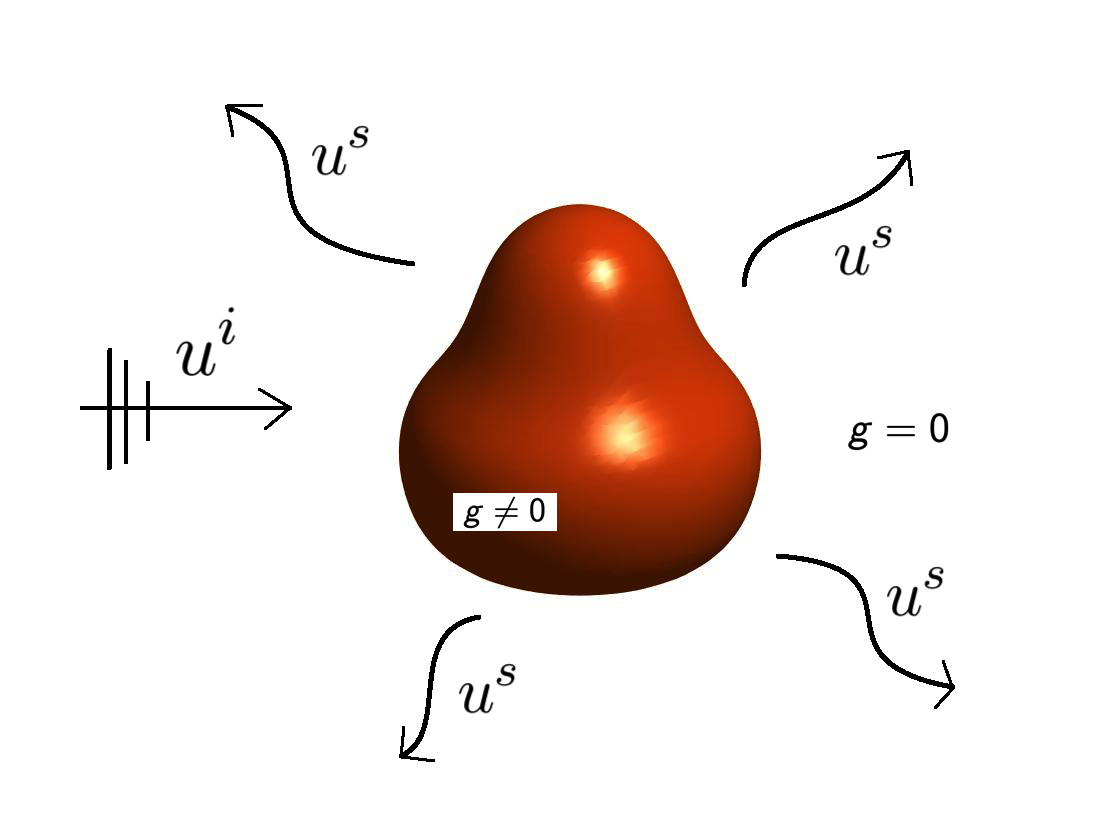
Figure 1: Inverse scattering problems.

Despite numerous studies on inverse problems, most of the existing results in the literature are not applicable for making inferences about unknown functional inputs, including the estimation and its uncertainty quantification. Recent developments for functional inputs have primarily relied on the idea of truncated basis expansion (Tan,, 2019; Li and Tan,, 2022), which is intuitive and commonly used in functional data analysis but can result in inefficient estimation and additional uncertainty in the inverse estimation. To successfully address the inverse problems with functional inputs, a critical yet challenging step is to construct efficient surrogate models for mathematical forward solvers that can accurately capture the information from functional inputs and provide rigorous quantification of the prediction uncertainty.

Motivated by an inverse scattering problem where the functional input of interest is the refractive index over a bounded scatterer, a novel Bayesian framework is proposed. This framework tackles the aforementioned challenges by constructing an efficient surrogate model that directly accounts for the functional inputs and a Bayesian procedure that allows efficient and accurate inference of the functional inverse through the posterior distribution. In particular, the surrogate model is constructed by a Gaussian process prior with functional inputs, which captures the information from the functional input directly through kernel functions without finite basis expansion, thereby retaining the information without any truncation. Furthermore, this surrogate model is used to efficiently integrate multi-fidelity simulations, including low-fidelity simulations (such as Born approximation) and high-fidelity simulations (such as nonlinear equations solved by finite element methods), to achieve better reconstruction accuracy and computational efficiency. While there have been numerous developments on multi-fidelity emulation (Kennedy and O’Hagan,, 2000), most of the existing work focuses on scalar inputs and the extensions to functional inputs are nontrivial.

Note that, identifying the functional inverse in the current setting is different from the calibration of computer models with functional parameters in recent studies (Plumlee et al.,, 2016; Brown and Atamturktur,, 2018; Tuo et al.,, 2021; Sung,, 2022). The calibration parameters of interest in those studies were represented as functions of control variables, and each model output was generated through a scalar parameter assumed to be a realization of an unknown function $g(x)$. In contrast, the inverse scattering problem herein involves a single function $g$, which is explicitly given (e.g., $g(x)=1+x$), that generates only one response pattern in the computer model. Consequently, there is significantly less information available to guide the search for the inverse in the functional space, leading to a more challenging problem.

The remainder of the paper is organized as follows. Section 2 introduces the Bayesian framework for the inverse scattering problem when only one numerical simulator is available. In Section 3, we propose a method to reconstruct the inverse function by integrating multi-fidelity simulators. Section 4 presents the results of inverse prediction and uncertainty quantification for the refractive index of a bounded scatterer. Finally, in Section 5, we conclude with future research directions. Detailed algorithms are provided in Appendix, and the R (R Core Team,, 2018) code for reproducing numerical results is provided in Supplemental Materials.

2 Bayesian inference for functional inverse

Suppose that $V$ is a functional input space consisting of functions defined on a compact and convex region $\Omega\subseteq\mathbb{R}^{d}$, and all functions $g(\mathbf{x})\in V$ are continuous in $\Omega$, where $\mathbf{x}\in\Omega$. Given a functional input $g(\mathbf{x})\in V$, $\mathbf{y}^{s}(g)$ is the corresponding output obtained from a forward mathematical solver which is often computationally intensive, such as a series of nonlinear partial differential equations solved by finite element methods (FEMs). For each functional input, the output is typically an image and it can be vectorized as a vector with length $m$, thus we have $\mathbf{y}^{s}:V\rightarrow\mathbb{R}^{m}$. For example, based on the ten training input functions shown in the panel titles of Figure 2, the corresponding ten outputs $\mathbf{y}^{s}(g)$ are given in image format as in Figure 2, which can be viewed as a vector of length $m=1024$. Let $\mathbf{y}^{p}$ be a vector of the observed far-field pattern. It is assumed that

$$\mathbf{y}^{p}=\mathbf{y}^{s}(g)+\mathbf{e},$$ (1)

where $\mathbf{e}$ is the random noise and each of its element follows an identical, independent normal distribution with zero mean and variance $\sigma^{2}_{e}$, i.e., $\mathbf{e}\sim\mathcal{N}_{m}(\mathbf{0}_{m},\sigma^{2}_{e}\mathbf{I}_{m})$ and $\mathbf{I}_{m}$ is an identity matrix of size $m$. Based on a training set received from mathematical forward solvers, the objective in inverse scattering is to reconstruct the functional input $g$ corresponding to the received far-field pattern.

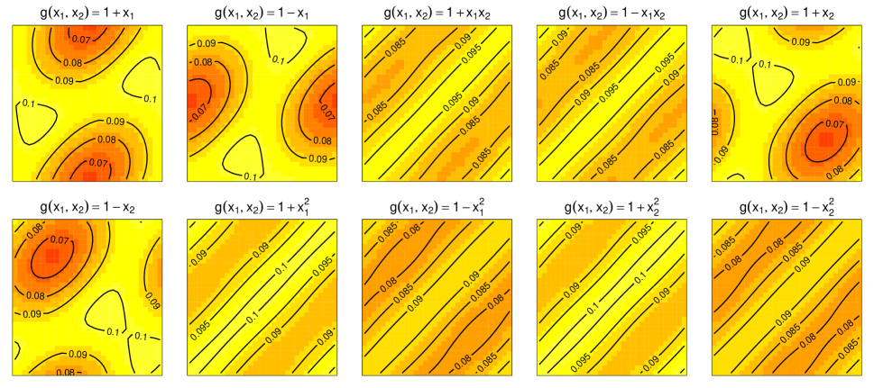
Figure 2: Training data from finite-element simulations, where the functional inputs are given in the panel titles and the images are their corresponding far-field outputs.

To develop a Bayesian approach for inverse scattering problems, a surrogate model for mathematical solvers is first introduced in Section 2.1 to efficiently emulate $\mathbf{y}^{s}(g)$ with functional inputs. This step is crucial because mathematical solvers are typically computationally intensive; therefore, it is infeasible to explore the entire functional input space by mathematical solvers. Based on (1) and the surrogate model constructed in Section 2.1, a Bayesian framework for inverse scattering is proposed in Section 2.2.

2.1 Surrogate model with functional inputs

Since the response far-field patterns $\mathbf{y}^{s}(g)$ are images, we first pre-process the images by a dimension reduction method. Specifically, principal component analysis (PCA) is performed to identify the first $L$ principal components, $\mathbf{u}_{l}\in\mathbb{R}^{1024},l=1,2,\ldots,L$, that explain more than $99\%$ of the variability of the images in the training set. As a result, given the functional input $g_{i}$ for $i=1,\ldots,n$, the output of the far-field images can be approximated by

$$\mathbf{y}^{s}(g_{i})\approx\sum^{L}_{l=1}f_{l}(g_{i})\mathbf{u}_{l},$$ (2)

where $\{f_{l}(g_{i})\}^{L}_{l=1}$ are the first $L$ principal component scores, which are computed by $f_{l}(g_{i})=\mathbf{u}^{T}_{l}\mathbf{y}^{s}(g_{i})$. After the dimension reduction, instead of modeling the output images, the objective becomes to construct an efficient surrogate model that predicts the principal component scores $f_{l}(g)$ for any $g\in V$.

Gaussian process (GP) models (Santner et al.,, 2018; Gramacy,, 2020) are widely used to construct statistical surrogates for mathematical solvers, but building a surrogate for $f_{l}(g)$ is challenging when the input $g$ is in a functional form instead of a scalar input. This is because a new kernel function, denoted by $K_{l}(g,g^{\prime})$ with $g,g^{\prime}\in V$, is needed to describe the correlation structure in a functional space directly. To this end, we adopt the functional-input GP model proposed by Sung et al., (2023):

$$f_{l}(g)\sim\mathcal{FIGP}(\mu_{l},K_{l}(g,g^{\prime})),$$

where $\mu_{l}$ is an unknown mean, $K_{l}(g,g^{\prime})$ is semi-positive definite, and $\{f_{l}(g)\}^{L}_{l=1}$ are assumed to be mutually independent. As introduced by Sung et al., (2023), there are two classes of kernel functions for any functional inputs $g_{1},g_{2}\in V$, including a linear kernel :

$$K_{l}(g_{1},g_{2})=\tau^{2}_{l}\int_{\Omega}\int_{\Omega}g_{1}(\mathbf{x})g_{2}(\mathbf{x}^{\prime})\Phi_{\boldsymbol{\theta}_{l}}(\mathbf{x},\mathbf{x}^{\prime}){\rm{d}}\mathbf{x}{\rm{d}}\mathbf{x}^{\prime},$$ (3)

and a nonlinear kernel:

$$K_{l}(g_{1},g_{2})=\tau^{2}_{l}\phi(\gamma_{l}\|g_{1}-g_{2}\|_{L_{2}(\Omega)}),$$ (4)

where $\tau_{l}^{2}$ is a positive scalar, $\Phi_{\boldsymbol{\theta}_{l}}$ is a positive definite kernel function defined on $\Omega\times\Omega$ with the hyperparameter $\boldsymbol{\theta}_{l}$, $\phi(r):\mathbb{R}^{+}\rightarrow\mathbb{R}$ is a radial basis function whose corresponding kernel in $\mathbb{R}^{d}$ is strictly positive definite for any $d\geq 1$, $\|\cdot\|_{L_{2}(\Omega)}$ is the $L_{2}$-norm of a function, defined by $\|h\|_{L_{2}(\Omega)}=(\langle h,h\rangle_{L_{2}(\Omega)})^{1/2}$, and $\gamma_{l}>0$ is a parameter that controls the decay of the kernel function with respect to the $L_{2}$-norm. Throughout this paper, the kernel function $\Phi_{\boldsymbol{\theta}_{l}}$ is assumed to be a Matérn kernel, which is widely used in the literature (Santner et al.,, 2018; Stein,, 1999). The Matérn kernel function has the form of

$$\Phi_{\boldsymbol{\theta}_{l}}(\mathbf{x},\mathbf{x}^{\prime})=\phi(\|\boldsymbol{\theta}_{l}\odot(\mathbf{x}-\mathbf{x}^{\prime})\|_{2})$$ (5)

with the Matérn radial basis function:

$$\phi(r)=\frac{1}{\Gamma(\nu)2^{\nu-1}}(2\sqrt{\nu}r)^{\nu}B_{\nu}(2\sqrt{\nu}r),$$ (6)

where $\odot$ is the Hadamard product, and $\boldsymbol{\theta}_{l}$ is a lengthscale parameter of length $d$, $\|\cdot\|_{2}$ denotes the Euclidean norm, $B_{\nu}$ is the modified Bessel function of the second kind, and $\nu$ represents a smoothness parameter. Quasi-Monte Carlo integration (Morokoff and Caflisch,, 1995) can be used to numerically evaluate the integrals in the kernels. Specifically, suppose that $\Omega$ is a unit cube, then the linear kernel (3) can be approximated by

$$K_{l}(g_{1},g_{2})\approx\frac{\tau^{2}_{l}}{N^{2}}\left(\mathbf{g}^{T}_{1,N}\boldsymbol{\Phi}_{\boldsymbol{\theta}_{l}}\mathbf{g}_{2,N}\right),$$ (7)

where $\boldsymbol{\Phi}_{\boldsymbol{\theta}_{l}}$ is an $N\times N$ matrix with each element $(\boldsymbol{\Phi}_{\boldsymbol{\theta}_{l}})_{i,j}=\Phi_{\boldsymbol{\theta}_{l}}(\mathbf{x}_{i},\mathbf{x}_{j})$, $\mathbf{g}_{j,N}$ is a vector of length $N$, which is $\mathbf{g}_{j,N}=(g_{j}(\mathbf{x}_{1}),\ldots,g_{j}(\mathbf{x}_{N}))^{T}$, and $\{\mathbf{x}_{i}\}^{N}_{i=1}$ is a low-discrepancy sequence from a unit cube, for which the Sobol sequence (Sobol’,, 1967; Bratley and Fox,, 1988) is adopted here.

Based on a selected kernel function, the $n$ outputs ($f_{l}(g_{1}),\ldots,f_{l}(g_{n})$) follow a multivariate normal distribution,

$$\mathbf{f}_{l}:=(f_{l}(g_{1}),\ldots,f_{l}(g_{n}))^{T}\sim\mathcal{N}_{n}(\mu_{l}\boldsymbol{1}_{n},\mathbf{K}_{l}),$$

where the covariance $\mathbf{K}_{l}\in\mathbb{R}^{n\times n}$ with $(\mathbf{K}_{l})_{j,k}=K_{l}(g_{j},g_{k})$, and $\boldsymbol{1}_{n}$ is a size-$n$ all-ones vector. Denote $\mathbf{Y}_{s}=(\mathbf{y}^{s}(g_{1}),\ldots,\mathbf{y}^{s}(g_{n}))\in\mathbb{R}^{m\times n}$, which implies that $\mathbf{f}_{l}=\mathbf{Y}^{T}_{s}\mathbf{u}_{l}$. The unknown parameters, including $\mu_{l}$ and the hyperparameters associated with the kernel function, which are either $\boldsymbol{\theta}_{l}$ in (3) or $\gamma_{l}$ in (4), can be estimated by maximizing the log-likelihood function:

$$\text{constant}-\frac{1}{2}\log|\mathbf{K}_{l}|-\frac{1}{2}(\mathbf{Y}^{T}_{s}\mathbf{u}_{l}-\mu_{l}\boldsymbol{1}_{n})^{T}\mathbf{K}_{l}^{-1}(\mathbf{Y}^{T}_{s}\mathbf{u}_{l}-\mu_{l}\boldsymbol{1}_{n}).$$

The choice of the kernel function depends on the complexity of the underlying structure. To find the kernel function that balances the bias–variance trade-off in practice, the idea of leave-one-out cross-validation (LOOCV) suggested by Sung et al., (2023) is implemented, which provides an efficient closed-form expression to select the kernel by minimizing the estimated prediction error:

$$\text{LOOCV}=\frac{1}{n}\|\boldsymbol{\Lambda}_{l}^{-1}\mathbf{K}_{l}^{-1}(\mathbf{Y}^{T}_{s}\mathbf{u}_{l}-\mu_{l}\boldsymbol{1}_{n})\|^{2}_{2},$$ (8)

where $\boldsymbol{\Lambda}_{l}\in\mathbb{R}^{n\times n}$ is a diagonal matrix with the element $(\boldsymbol{\Lambda}_{l})_{j,j}=(\mathbf{K}_{l}^{-1})_{j,j}$.

By the property of the conditional multivariate normal distribution, the corresponding output $f_{l}(g)$ for an untried functional input, $g\in V$, follows a normal distribution

$$f_{l}(g)|\mathbf{Y}_{s}\sim\mathcal{N}(m_{l}(g),v_{l}(g))$$ (9)

with

$$m_{l}(g)=\mu_{l}+\mathbf{k}_{l}(g)^{T}\mathbf{K}^{-1}_{l}(\mathbf{Y}^{T}_{s}\mathbf{u}_{l}-\mu_{l}\boldsymbol{1}_{n})$$ (10)

and

$$v_{l}(g)=K_{l}(g,g)-\mathbf{k}_{l}(g)^{T}\mathbf{K}^{-1}_{l}\mathbf{k}_{l}(g),$$ (11)

where $\mathbf{k}_{l}(g)=(K_{l}(g,g_{1}),...,K_{l}(g,g_{n}))^{T}\in\mathbb{R}^{n\times 1}$. Hence, since $\mathbf{y}^{s}(g_{i})\approx\sum^{L}_{l=1}f_{l}(g_{i})\mathbf{u}_{l}$, the surrogate model $\mathbf{y}^{s}(g)$ follows a multivariate normal distribution as

$$\mathbf{y}^{s}(g)\sim\mathcal{N}_{m}\left(\sum^{L}_{l=1}m_{l}(g)\mathbf{u}_{l},\sum^{L}_{l=1}v_{l}(g)\mathbf{u}_{l}\mathbf{u}^{T}_{l}\right).$$ (12)

2.2 Bayesian approach for functional inverse

Given the output $\mathbf{y}^{p}$ in the model (1), we assume that the unknown functional inverse follows a GP prior. By combining (1), (12), and the prior information, the following Bayesian framework is considered,

$$\mathbf{y}^{p}|g,\sigma^{2}_{e} \sim\mathcal{N}_{m}\left(\sum^{L}_{l=1}m_{l}(g)\mathbf{u}_{l},\sigma^{2}_{e}\mathbf{I}_{m}+\sum^{L}_{l=1}v_{l}(g)\mathbf{u}_{l}\mathbf{u}^{T}_{l}\right),$$ (13)

$$g(\mathbf{x})|\boldsymbol{\eta},\sigma^{2}_{g} \sim\mathcal{GP}(0,\tau^{2}_{g}\Phi_{\boldsymbol{\eta}}(\mathbf{x},\mathbf{x}^{\prime})),$$ (14)

$$\sigma^{2}_{e} \sim\text{InvGamma}(a_{1},b_{1}),$$ (15)

$$\tau^{2}_{g} \propto\text{InvGamma}(a_{2},b_{2}),$$ (16)

$$\eta_{j} \propto\text{Gamma}(a_{3},b_{3})\quad\text{for}\quad j=1,\ldots,d,$$ (17)

where $\text{InvGamma}(a,b)$ denotes an inverse gamma distribution with shape parameter $a$ and rate parameter $b$. In (14), we assume that the functional input $g$ follows a GP prior, denoted by $\mathcal{GP}$, where $\Phi_{\boldsymbol{\eta}}$ is a Matérn kernel as in (5) with the lengthscale parameter $\boldsymbol{\eta}$. The prior distributions of the parameters $\sigma_{e}^{2}$, $\tau_{g}^{2}$, and $\boldsymbol{\eta}$ are given in (15), (16), and (17), respectively.

Note that the GP prior is also used to model parameters or inputs that are represented as a function in the literature of inverse problems; however, most of existing works consider a truncated Karhunen–Loève (KL) expansion to reduce the dimension of the GP prior (Marzouk and Najm,, 2009; Li and Tan,, 2022; Yang et al.,, 2017). In contrast, the proposed model employs a GP prior that includes a prior density for the lengthscale parameter as in (17) and avoids basis expansion and truncation, which is important because finite truncation associated with basis expansion can introduce model bias. In addition, based on the proposed emulator (12), the functional-input emulator is modeled directly through kernel functions without finite basis expansion. Therefore, the input information is better preserved compared to Tan, (2019) and Li and Tan, (2022), where the emulator is built based on a finite basis expansion of the functional inputs. Numerical comparisons are available in Section 4.

The computation involved in the likelihood function of (13) can further be simplified as follows. By the Woodbury matrix identity (Harville,, 1998) and the fact that $\mathbf{u}^{T}_{l}\mathbf{u}_{l}=1$ and $\mathbf{u}^{T}_{l}\mathbf{u}_{l^{\prime}}=0$ for any $l\neq l^{\prime}$, the covariance inverse of (13) can be written as

$$\left(\sigma^{2}_{e}\mathbf{I}_{m}+\sum^{L}_{l=1}v_{l}(g)\mathbf{u}_{l}\mathbf{u}^{T}_{l}\right)^{-1}=\frac{1}{\sigma^{2}_{e}}\mathbf{I}_{m}-\frac{1}{\sigma^{2}_{e}}\mathbf{U}\left(\sigma^{2}_{e}\mathbf{V}_{L}(g)^{-1}+\mathbf{I}_{L}\right)^{-1}\mathbf{U}^{T}$$

where $\mathbf{V}_{L}(g)\in\mathbb{R}^{L\times L}$ is a diagonal matrix with each element $(\mathbf{V}_{L}(g))_{l}=v_{l}(g)$, and the determinant of the covariance can be simplified as

$$\text{det}\left(\sigma^{2}_{e}\mathbf{I}_{m}+\sum^{L}_{l=1}v_{l}(g)\mathbf{u}_{l}\mathbf{u}^{T}_{l}\right)=(\sigma_{e}^{2})^{m}\prod^{L}_{l=1}\left(1+\frac{v_{l}(g)}{\sigma_{e}^{2}}\right).$$

As a result, the likelihood function of (13) can be written as

$$L(\mathbf{y}^{p}|g,\sigma^{2}_{e})\propto (\sigma_{e}^{2})^{-\frac{m}{2}}\prod^{L}_{l=1}\left(1+\frac{v_{l}(g)}{\sigma_{e}^{2}}\right)^{-1/2}\times$$

$$\exp\left\{-\frac{1}{2\sigma^{2}_{e}}\left(\left\|\mathbf{y}^{p}-\sum^{L}_{l=1}m_{l}(g)\mathbf{u}_{l}\right\|^{2}_{2}-\sum^{L}_{l=1}\frac{(\mathbf{u}^{T}_{l}\mathbf{y}^{p}-m_{l}(g))^{2}}{\sigma^{2}_{e}/v_{l}(g)+1}\right)\right\}.$$ (18)

The expression in (2.2) allows the likelihood function of (13) to be computed easily because it circumvents the need of the $m\times m$ matrix inversion associated with the $m$-dimensional multivariate normal distribution.

To evaluate the likelihood function $L(\mathbf{y}_{n}^{p}|g,\sigma^{2}_{e})$, the function $g$ is replaced by its realization $\mathbf{g}_{N}=(g(\mathbf{x}_{1}),\ldots,g(\mathbf{x}_{N}))^{T}$ at a low-discrepancy sequence $\mathbf{X}_{N}=\{\mathbf{x}_{i}\}^{N}_{i=1}$, which enables the evaluations of $m_{l}(g)$ and $v_{l}(g)$ in the likelihood function, in which the kernel function $\mathbf{k}_{l}(g)$ of (10) and (11) is approximated based on $\mathbf{g}_{N}$ as in (7). Thus, given the observation $\mathbf{y}^{p}$, the posterior of the functional input $g(\mathbf{x})$ can be obtained by

$$\pi(g(\mathbf{x}),\mathbf{g}_{N},\sigma^{2}_{e},\boldsymbol{\eta},\tau^{2}_{g}|\mathbf{y}^{p})\propto\pi(g(\mathbf{x})|\mathbf{g}_{N},\boldsymbol{\eta},\tau^{2}_{g})\pi(\mathbf{g}_{N},\sigma^{2}_{e},\boldsymbol{\eta},\tau^{2}_{g}|\mathbf{y}^{p}).$$ (19)

The joint posterior distribution of $g(\mathbf{x})$ can be approximated by Markov chain Monte Carlo (MCMC) by drawing the samples from $\pi(g(\mathbf{x})|\mathbf{g}_{N},\boldsymbol{\eta},\tau^{2}_{g})$ and $\pi(\mathbf{g}_{N},\sigma^{2}_{e},\boldsymbol{\eta},\tau^{2}_{g}|\mathbf{Y}_{n}^{p})$, iteratively. For the posterior $\pi(\mathbf{g}_{N},\sigma^{2}_{e},\boldsymbol{\eta},\sigma^{2}_{g}|\mathbf{y}^{p})$, it follows that

$$\pi(\mathbf{g}_{N},\sigma^{2}_{e},\boldsymbol{\eta},\tau^{2}_{g}|\mathbf{y}^{p})\propto L(\mathbf{y}_{n}^{p}|\mathbf{g}_{N},\sigma^{2}_{e})\pi(\mathbf{g}_{N}|\boldsymbol{\eta},\tau^{2}_{g})\pi(\sigma^{2}_{e})\pi(\boldsymbol{\eta})\pi(\tau^{2}_{g})$$ (20)

where $L(\mathbf{y}_{n}^{p}|\mathbf{g}_{N},\sigma^{2}_{e})$ is the likelihood function (2.2) with the realization $\mathbf{g}_{N}$, $\pi(\mathbf{g}_{N}|\boldsymbol{\eta},\tau^{2}_{g})$ follows $\mathcal{N}_{N}(\mathbf{0}_{N},\tau^{2}_{g}\boldsymbol{\Phi}_{\boldsymbol{\eta}})$ based on the GP prior (14), where $\boldsymbol{\Phi}_{\boldsymbol{\eta}}$ is an $N\times N$ matrix with each element $(\boldsymbol{\Phi}_{\boldsymbol{\eta}})_{i,j}=\Phi_{\boldsymbol{\eta}}(\mathbf{x}_{i},\mathbf{x}_{j})$, and $\pi(\sigma^{2}_{e})$, $\pi(\boldsymbol{\eta})$, and $\pi(\tau^{2}_{g})$ are the priors as in (15), (16), and (17). The samples from this posterior distribution can be drawn by Gibbs sampling with Metropolis-Hastings algorithm. The details are given in Appendix A.

The posterior $\pi(g(\mathbf{x})|\mathbf{g}_{N},\boldsymbol{\eta},\tau^{2}_{g})$ can be drawn based on the property of conditional multivariate normal distributions, that is,

$$g(\mathbf{x})|\mathbf{g}_{N},\boldsymbol{\eta},\tau^{2}_{g}\sim\mathcal{N}(\Phi_{\boldsymbol{\eta}}(\mathbf{x},\mathbf{X}_{N})\boldsymbol{\Phi}_{\boldsymbol{\eta}}^{-1}\mathbf{g}_{N},\tau^{2}_{g}(1-\Phi_{\boldsymbol{\eta}}(\mathbf{x},\mathbf{X}_{N})\boldsymbol{\Phi}_{\boldsymbol{\eta}}^{-1}\Phi_{\boldsymbol{\eta}}(\mathbf{X}_{N},\mathbf{x}))),$$

where $\Phi_{\boldsymbol{\eta}}(\mathbf{x},\mathbf{X}_{N})=(\Phi_{\boldsymbol{\eta}}(\mathbf{x},\mathbf{x}_{1}),\ldots,\Phi_{\boldsymbol{\eta}}(\mathbf{x},\mathbf{x}_{N}))$, and $\Phi_{\boldsymbol{\eta}}(\mathbf{X}_{N},\mathbf{x})=\Phi_{\boldsymbol{\eta}}(\mathbf{x},\mathbf{X}_{N})^{T}$.

Similarly, the posterior of $\mathbf{y}^{s}(g)$ given $\mathbf{y}^{p}$ and $\mathbf{Y}_{s}$ can be obtained by

$$\pi(\mathbf{y}^{s}(g),\mathbf{g}_{N},\sigma^{2}_{e},\boldsymbol{\eta},\tau^{2}_{g}|\mathbf{y}^{p},\mathbf{Y}_{s})\propto\pi(\mathbf{y}^{s}(g)|\mathbf{g}_{N},\mathbf{Y}_{s})\pi(\mathbf{g}_{N},\sigma^{2}_{e},\boldsymbol{\eta},\tau^{2}_{g}|\mathbf{y}^{p}),$$ (21)

where the samples from $\pi(\mathbf{g}_{N},\sigma^{2}_{e},\boldsymbol{\eta},\tau^{2}_{g}|\mathbf{y}^{p})$ can be drawn as in (20), and the samples from $\pi(\mathbf{y}^{s}(g)|\mathbf{g}_{N},\mathbf{Y}_{s})$ can be drawn the multivariate normal distribution (12) with the realization $\mathbf{g}_{N}$ for evaluating the kernel functions.

3 Surrogate model for multi-fidelity solvers with functional inputs

Section 2 focuses on the situations where only one solver is available for the inverse scattering problem. In practice, there are often multiple solvers available with different accuracy and different computational efficiency. Accurate forward solvers, also known as high-fidelity simulators, involve nonlinear differential equations that are solved by FEMs, which are often prohibitively costly to have sufficient training samples to explore the functional input space. On the other hand, linearized approximations, such as Born approximation (Kazei and Alkhalifah,, 2018; Muhumuza et al.,, 2018), are low-fidelity solvers, which are developed to serve as faster alternatives, although they are less accurate compared to the high-fidelity simulators. Figure 3 presents the far-field patterns simulated based on Born approximation, which are computationally faster to obtain than the FEM simulations shown in Figure 2 but less accurate. A new Bayesian framework, extending from Section 2, is introduced to infer functional inverse in scattering problems by integrating multi-fidelity simulations. We denote the high-fidelity simulator as $\mathbf{y}^{s}(g)$ and denote the low-fidelity simulator as $\mathbf{y}^{b}(g)$.

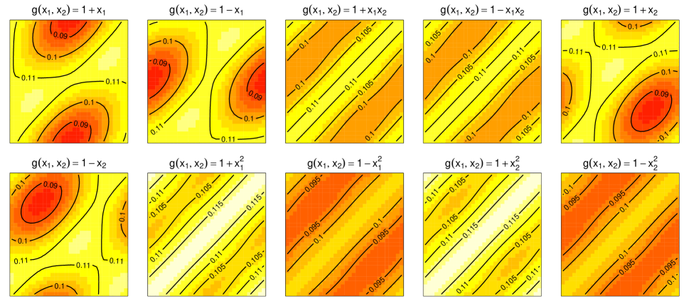
Figure 3: Training data of Born approximation simulator, where the functional inputs are given in the titles and the images are their corresponding far-field outputs.

Similar to Section 2, we apply PCA to the image output $\mathbf{y}^{b}(g)$, where the principal component scores are obtained by $h_{l}(g)=\mathbf{u}^{T}_{l}\mathbf{y}^{b}(g)$ with the principal component $\mathbf{u}_{l}$ given in (2) for $l=1,\ldots,L$. To emulate the high-fidelity simulator, we assume an autoregressive model that integrates the multi-fidelity solvers:

$$f_{l}(g)=\rho_{l}h_{l}(g)+\delta_{l}(g),$$ (22)

where $\rho_{l}$ is an unknown parameter and $\delta_{l}(g)$ is the unknown discrepancy between high-fidelity and low-fidelity simulators. The model can be viewed as an extension of the autoregressive model proposed by Kennedy and O’Hagan, (2000) to functional inputs. Similar to the idea in Section 2, $h_{l}(g)$ and $\delta_{l}(g)$ are modeled as a functional-input GP (Sung et al.,, 2023), i.e.,

$$h_{l}(g)\sim\mathcal{FIGP}(\mu_{h_{l}},K_{h_{l}}(g,g^{\prime}))\quad\text{and}\quad\delta_{l}(g)\sim\mathcal{FIGP}(\mu_{\delta_{l}},K_{\delta_{l}}(g,g^{\prime}))$$ (23)

for $l=1,\ldots,L$, and assume that $\{h_{l}(g)\}^{L}_{l=1}$ and $\{\delta_{l}(g)\}^{L}_{l=1}$ are mutually independent. The definitions of $\mu_{h_{l}},\mu_{\delta_{l}},K_{h_{l}}$ and $K_{\delta_{l}}$ are similar to the ones defined in Section 2.1. Thus, it follows that

$$(h_{l}(g_{1}),\ldots,h_{l}(g_{n}))^{T}\sim\mathcal{N}_{n}(\mu_{h_{l}}\mathbf{1}_{n},\mathbf{K}_{h_{l}})\quad\text{and}\quad(\delta_{l}(g_{1}),\ldots,\delta_{l}(g_{n}))^{T}\sim\mathcal{N}_{n}(\mu_{\delta_{l}}\mathbf{1}_{n},\mathbf{K}_{\delta_{l}}),$$

where $(\mathbf{K}_{h_{l}})_{j,k}=K_{h_{l}}(g_{j},g_{k})$ and $(\mathbf{K}_{\delta_{l}})_{j,k}=K_{\delta_{l}}(g_{j},g_{k})$. Since $\delta_{l}(g_{i})=f_{l}(g_{i})-\rho_{l}h_{l}(g_{i})=\mathbf{u}^{T}_{l}(\mathbf{y}^{s}(g_{i})-\rho_{l}\mathbf{y}^{b}(g_{i}))$, the parameters, $\rho_{l},\mu_{\delta_{l}}$ and the parameters associated with the kernel $K_{\delta_{l}}$, can be estimated by maximizing the log-likelihood function,

$$\text{constant}-\frac{1}{2}\log|\mathbf{K}_{\delta_{l}}|-\frac{1}{2}((\mathbf{Y}_{s}-\rho_{l}\mathbf{Y}_{b})^{T}\mathbf{u}_{l}-\mu_{\delta_{l}}\boldsymbol{1}_{n})^{T}\mathbf{K}_{\delta_{l}}^{-1}((\mathbf{Y}_{s}-\rho_{l}\mathbf{Y}_{b})^{T}\mathbf{u}_{l}-\mu_{\delta_{l}}\boldsymbol{1}_{n}),$$

where $\mathbf{Y}_{b}=(\mathbf{y}^{b}(g_{1}),\ldots,\mathbf{y}^{b}(g_{n}))\in\mathbb{R}^{m\times n}$. The parameter, $\mu_{h_{l}}$, and the parameters of the kernel $K_{h_{l}}$, can be estimated by maximizing the log-likelihood function,

$$\text{constant}-\frac{1}{2}\log|\mathbf{K}_{h_{l}}|-\frac{1}{2}(\mathbf{Y}_{b}^{T}\mathbf{u}_{l}-\mu_{h_{l}}\boldsymbol{1}_{n})^{T}\mathbf{K}_{h_{l}}^{-1}(\mathbf{Y}_{b}^{T}\mathbf{u}_{l}-\mu_{h_{l}}\boldsymbol{1}_{n}).$$

By the property of the conditional multivariate normal distribution, the corresponding output $f_{l}(g)$ for an untried input, $g\in V$, follows a normal distribution

$$f_{l}(g)|\mathbf{Y}_{s},\mathbf{Y}_{b}\sim\mathcal{N}(m^{(b)}_{l}(g),v^{(b)}_{l}(g))$$ (24)

with

$$m^{(b)}_{l}(g)=(\rho_{l}\mu_{h_{l}}+\mu_{\delta_{l}})+\mathbf{t}_{l}(g)^{T}\mathbf{V}_{l}^{-1}(\mathbf{z}_{l}-\boldsymbol{\mu}_{l})$$

and

$$v^{(b)}_{l}(g)=\rho^{2}_{l}K_{h_{l}}(g,g)+K_{\delta_{l}}(g,g)-\mathbf{t}_{l}(g)^{T}\mathbf{V}_{l}^{-1}\mathbf{t}_{l}(g),$$

where

$$\mathbf{z}_{l}=\left(\begin{array}[]{c}\mathbf{Y}^{T}_{b}\mathbf{u}_{l}\\ \mathbf{Y}^{T}_{s}\mathbf{u}_{l}\end{array}\right),\quad\boldsymbol{\mu}_{l}=\left(\begin{array}[]{c}\mu_{h_{l}}\mathbf{1}_{n}\\ (\rho_{l}\mu_{h_{l}}+\mu_{\delta_{l}})\mathbf{1}_{n}\end{array}\right),$$

$$\mathbf{V}_{l}=\left(\begin{array}[]{cc}\mathbf{K}_{h_{l}}&\rho_{l}\mathbf{K}_{h_{l}}\\ \rho_{l}\mathbf{K}_{h_{l}}&\rho^{2}_{l}\mathbf{K}_{h_{l}}+\mathbf{K}_{\delta_{l}}\end{array}\right),\quad\mathbf{t}_{l}(g)=\left(\begin{array}[]{c}\rho_{l}\mathbf{k}_{h_{l}}(g)\\ \rho_{l}^{2}\mathbf{k}_{h_{l}}(g)+\mathbf{k}_{\delta_{l}}(g)\end{array}\right),$$

where $\mathbf{k}_{h_{l}}(g)=(K_{h_{l}}(g,g_{1}),...,K_{h_{l}}(g,g_{n}))^{T}$ and $\mathbf{k}_{\delta_{l}}(g)=(K_{\delta_{l}}(g,g_{1}),...,K_{\delta_{l}}(g,g_{n}))^{T}$.

According to (24), the Bayesian framework developed in Section 2 can be easily extended to integrate multi-fidelity simulators by replacing the mean $m_{l}(g)$ and variance $v_{l}(g)$ by $m_{l}^{(b)}(g)$ and $v_{l}^{(b)}(g)$ respectively.

4 Applications to Inverse Scattering Problems

The inverse scattering problem introduced in Section 1 is revisited and analyzed by the proposed Bayesian framework. Based on the training set simulated from mathematical models, the objective is to infer the functional input, given an observed far-field pattern. The functional input $g$ in this study represents the refractive index of the bounded medium as shown in the middle of Figure 1. The proposed Bayesian approach is implemented to determine the refractive index $g$ where the estimation uncertainty is measured using its posterior distribution. Two analysis results are presented in Sections 4.1 and 4.2, with one analysis based solely on FEM simulators and the other based on multi-fidelity simulations (FEM and Born approximation).

In this study, $\Omega\subseteq\mathbb{R}^{2}$, and 10 functional inputs of $g$, including $1,1+x_{1},1-x_{1},1+x_{1}x_{2},1-x_{1}x_{2},1+x_{2},1+x_{1}^{2},1-x_{1}^{2},1+x_{2}^{2}$, and $1-x_{2}^{2}$, are considered in the training set and their corresponding FEM simulations are shown in Figure 2. The PCA is first applied that yields the three principle components, $\mathbf{u}_{l}\in\mathbb{R}^{1024},l=1,2,3$, explaining more than 99.99% variability of the data, which are presented in Figure 4. The proposed method is tested on a functional input, $g(x_{1},x_{2})=1-\sin(x_{2})$, which is shown in the left panel of Figure 5, and its corresponding output $\mathbf{y}^{s}(g)$ is presented in the middle panel. The corresponding far-field pattern $\mathbf{y}^{p}$ is generated according to the model (1) with $\sigma^{2}_{e}=0.005^{2}$, which is shown in the right panel of Figure 5.

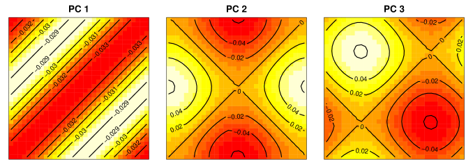
Figure 4: Principle components, which explain more than 99.99% variations of the data.

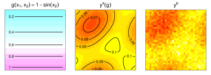
Figure 5: Illustration of the testing data. The underlying functional input (left), the FEM output (middle), and the observed far-field measurement (right).

The hyperparameters in the priors (15), (16), and (17) are set as follows: $a_{1}=a_{2}=a_{3}=1$ and $b_{1}=b_{3}=1$ and $b_{2}=10^{-5}$. The MCMC sampling involves 5000 iterations during a burn-in period, followed by an additional 5000 samples drawn and thinned to minimize autocorrelation. The Matérn kernel function with the smoothness parameter $\nu=5/2$ is considered, which leads to a simplified form of (6):

$$\phi(r)=\left(1+\sqrt{5}r+\frac{5}{3}r^{2}\right)\exp\left(-\sqrt{5}r\right).$$ (25)

The Sobol sequence (Sobol’,, 1967; Bratley and Fox,, 1988) of size $N=100$ is employed to approximate the kernel functions as in (7).

4.1 Inverse results with finite-element simulator

The functional-input GP introduced in Section 2.1 is implemented to construct the emulator based on the finite-element simulations $\{\mathbf{y}^{s}(g_{i})\}^{10}_{i=1}$ presented in Figure 2. The LOOCV criterion defined in (8) are computed for the functional-input GPs, $f_{1}(g),f_{2}(g)$ and $f_{3}(g)$, using the linear kernel (3) and nonlinear kernel (4). The results are summarized in Table 1, in which the linear kernel is suggested for all the three principal components.

	Kernel	$f_{1}(g)$	$f_{2}(g)$	$f_{3}(g)$
LOOCV	linear	$\boldsymbol{7.5\times 10^{-5}}$	$\boldsymbol{6.1\times 10^{-16}}$	$\boldsymbol{7.6\times 10^{-16}}$
	nonlinear	$8.1\times 10^{-5}$	$2.2\times 10^{-6}$	$1.9\times 10^{-6}$

Table 1: The leave-one-out cross-validation errors (LOOCVs) for each of the functional-input GPs, $f_{l}(g)$, based on the FEM simulations. The errors corresponding to the optimal kernel are boldfaced.

Based on the constructed emulator, the Bayesian approach developed in Section 2.2 is then applied to infer the functional inverse given the observed response wave shown in the right panel of Figure 5. Figure 6 demonstrates the progression of the MCMC algorithm in evaluating the posterior distribution of the functional inverse $g$ as in (19) and its corresponding predictive wave $\mathbf{y}^{s}(g)$ as in (21). As the algorithm progresses, both the sampled $g$ and the prediction of $\mathbf{y}^{s}(g)$ appear to be closer to the truth. The final posterior means of $g$ and $\mathbf{y}^{s}(g)$, demonstrated in the first and third panels of Figure 7, appear to accurately recover the true function $g$ and its output $\mathbf{y}^{s}(g)$, which are shown in Figure 5. Their posterior variances shown in the second and fourth panels of Figure 7 allow for quantifying the uncertainties associated with the inverse recovery and prediction, which appear to be reasonably small.

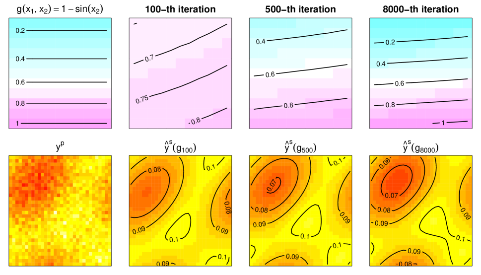
Figure 6: Demonstration of the MCMC algorithm. Upper panels show (for left to right) the true function $g$, and the sampled $g$ in the 100-th, 500-th, and 8000-th iterations of the MCMC algorithm. Lower panels show (for left to right) the physical far-field pattern $\mathbf{y}^{p}$, and the corresponding prediction means of $\mathbf{y}^{s}(g)$ with the sampled $g$.

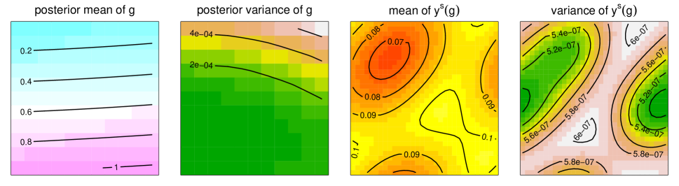
Figure 7: The inverse result based on the FEM simulator. The left two panels show the mean and variance of the MCMC samples of the function $g$, and the right two panels show the posterior mean and variance of $\mathbf{y}^{s}(g)$.

To examine the performance, the proposed method is compared with existing alternatives based on the idea of KL expansion with finite truncation, which is a common approach in functional data analysis. The performance is evaluated by the root-mean-square error (RMSE) and the average proper score, which is the scoring rule measuring the overall accuracy by taking into account both predictive mean and variance (Gneiting and Raftery,, 2007). Specifically, the proper score is defined as $-\left(\frac{y-\mu_{P}}{\sigma_{P}}\right)^{2}-\log\sigma^{2}_{P},$ where $y$ is the true output, $\mu_{P}$ is the predictive mean, and $\sigma^{2}_{P}$ is the predictive variance. The larger score indicates better prediction performance. The reconstruction performance of $g$, including the RMSE and proper score, is computed based on the realizations of the true function $g(x_{1},x_{2})=1-\sin(x_{2})$ and the posterior of $g$ on a set of grid points of size $101$ in the space $\Omega=[0,1]^{2}$.

Functional inputs are not only involved in constructing the emulator as discussed in Section 2.1, but also in the functional inverse developed in Section 2.2. To construct an emulator with functional inputs, the idea of truncated KL expansion is widely adopted in the literature of functional data analysis (Ramsay and Silverman,, 2005; Reiss et al.,, 2017; Yao and Müller,, 2010; Müller et al.,, 2013; Tan,, 2019). To recover the functional inverse, Li and Tan, (2022) propose to approximate the correlation function in the GP prior (14) by the expectation with respect to $\boldsymbol{\eta}$, which can be written as

$$C(\mathbf{x},\mathbf{x}^{\prime})=\int\Phi_{\boldsymbol{\eta}}(\mathbf{x},\mathbf{x}^{\prime})\pi(\boldsymbol{\eta})\rm{d}\boldsymbol{\eta},$$

and KL expansion and truncation are then applied to obtain the first few leading eigenfunctions of $C(\mathbf{x},\mathbf{x}^{\prime})$. Although this approximation leads to fast computation, it cannot flexibly capture different levels of underlying smoothness. Additionally, it can introduce additional model bias caused by the truncation from basis expansion.

Table 2 presents the numerical comparison of the proposed method with two different scenarios using the idea of KL-expansion. One applies KL-expansion to both emulator construction and functional inverse (the first row in Table 2), and the other only applies it to functional inverse (the second row in Table 2). The reconstructed inverse and the corresponding far-field predictions are shown in Figure 8. When the KL-expansion is applied to both emulator construction and inverse recovery (first row), the RMSE values for both functional recovery of $g$ and output prediction of $\mathbf{y}^{s}(g)$ are relatively large. When the KL expansion is replaced by the proposed FIGP (the second row) for constructing the emulator, the RMSE is significantly reduced as compared to the first row. This observation is consistent with the results shown in Figure 8, where the second row outperforms the first one in both inverse recovery and far-field prediction. This finding reveals the importance of preserving the functional input information through kernels as proposed in FIGP, as compared to KL-expansion where finite truncation introduces additional bias to the model. The third row represents the proposed method, FIGP+GP, where FIGP is utilized for emulator construction and GP is used for estimating the functional inverse. The results demonstrate that the proposed method outperforms the other two alternatives in terms of RMSEs and proper scores.

			recovered $g$		$\mathbf{y}^{s}(g)$
	emulator	inverse	RMSE	Score	RMSE	Score
FEM	KL	KL	0.815	-1.493	0.008572	8.73
	FIGP	KL	0.054	4.436	0.000571	6.67
	FIGP	GP	$\boldsymbol{0.028}$	5.623	0.000456	14.31
FEM + Born	FIGP	GP	0.033	$\boldsymbol{5.782}$	$\boldsymbol{0.000243}$	$\boldsymbol{15.857}$

Table 2: Performance of the recovered function $g$ and $\mathbf{y}^{s}(g)$ via single-fidelity simulations (FEM) and multi-fidelity simulations (FEM + Born). Better performances are highlighted as boldfaced.

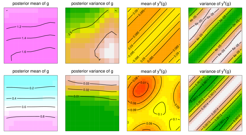
Figure 8: The results based on KL-expansion. The top row shows the results when KL-expansion is applied to both the emulator construction and functional inverse, which corresponds to the first row of Table 2. The bottom row shows the results when KL-expansion is applied to functional inverse, which corresponds to the second row of Table 2.

4.2 Inverse results with multi-fidelity simulation

In this subsection, the Bayesian framework with the multi-fidelity surrogate modeling developed in Section 3 is applied, which leverages the computational efficiency from the lower-fidelity simulations (Born approximation shown in Figure 3) to enhance predictions for the high-fidelity simulations (FEM shown in Figure 2). The functional-input GPs are applied as in (23), and the LOOCVs are computed for each of the functional-input GPs with a linear and nonlinear kernel, the results of which are summarized in Table 3. It shows that the linear kernel is preferred for the functional-input GPs $\{h_{l}(g)\}^{3}_{l=1}$, while the nonlinear kernel is preferred for $\{\delta_{l}(g)\}^{3}_{l=1}$. The estimated autoregressive parameters are $\hat{\rho}_{1}=0.62,\hat{\rho}_{2}=1.35$, and $\hat{\rho}_{3}=1.35$.

	Kernel	$h_{1}(g)$	$h_{2}(g)$	$h_{3}(g)$
LOOCV	linear	$\boldsymbol{6.3\times 10^{-16}}$	$\boldsymbol{4.1\times 10^{-16}}$	$\boldsymbol{4.2\times 10^{-16}}$
	nonlinear	$6.6\times 10^{-7}$	$1.2\times 10^{-6}$	$1.1\times 10^{-6}$
	Kernel	$\delta_{1}(g)$	$\delta_{2}(g)$	$\delta_{3}(g)$
LOOCV	linear	$7.5\times 10^{-5}$	$7.6\times 10^{-18}$	$9.5\times 10^{-20}$
	nonlinear	$\boldsymbol{6.8\times 10^{-5}}$	$\boldsymbol{7.3\times 10^{-18}}$	$\boldsymbol{8.9\times 10^{-20}}$

Table 3: The leave-one-out cross-validation errors (LOOCVs) for each of the functional-input GPs based on the multi-fidelity simulations. The errors corresponding to the optimal kernel are boldfaced.

The posterior means and variances of $g$ and $\mathbf{y}^{s}(g)$ are shown in Figure 9. It appears that both $g$ and $\mathbf{y}^{s}(g)$ are recovered fairly accurately with reasonably small uncertainties. The RMSE and average proper score are reported in the last row of Table 2. While it exhibits comparable performance to the single-fidelity simulator in reconstructing $g$ in terms of RMSE, utilizing the low-fidelity (Born approximation) simulations increases the proper score, which indicates the advantage of a smaller variation in the inverse reconstruction. Furthermore, integrating multi-fidelity simulations enhances the reconstruction accuracy of $\mathbf{y}^{s}(g)$, which leads to a smaller RMSE and a better proper score. This observation agrees with the findings in computer experiment literature (Kennedy and O’Hagan,, 2000; Sung et al.,, 2022). To sum up, the proposed Bayesian inverse method can provide accurate recovery of functional input $g$ in both single and multi-fidelity emulators.

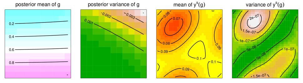
Figure 9: The inverse result based on the multi-fidelity simulator (FEM and Born approximation). The left two panels show the mean and variance of the MCMC samples of the function $g$, and the right two panels show the posterior mean and variance of $\mathbf{y}^{s}(g)$.

5 Concluding Remarks

The reconstruction of functional inverse in scattering problems is of increasing interest in science and engineering. In this article, a new Bayesian framework is introduced that includes a surrogate model, which accounts for functional inputs directly through kernel functions, and a hierarchical Bayesian procedure that infers functional inputs through the posterior distribution. The main contribution of the proposed method is the ability to prevent model bias caused by finite basis expansion, a common approach in functional data analysis, by employing a Gaussian process prior with linear and nonlinear kernels defined directly in the functional space. Furthermore, the proposed Bayesian approach integrates multi-fidelity simulations to enhance the accuracy for functional inverse reconstruction.

Besides MCMC discussed in the paper, it is of our interest to explore alternatives including variational Bayesian inference (Jordan et al.,, 1999; Wainwright and Jordan,, 2008; Tran et al.,, 2015; Hensman et al.,, 2015; Blei et al.,, 2017), which has the potential to speed up the computation and achieve a better scalability, particularly for large datasets. Another interesting ongoing research extended from the proposed method is the study of experimental designs in a functional space. Despite numerous studies on optimal design in computer experiments, the developments for functional inputs are scarce. In particular, the widely used space-filling designs in computer experiments are based on the distance measures defined in the Euclidean space, which are not directly applicable to a functional space. Furthermore, the development of efficient experimental designs for multi-fidelity simulations in a functional space is also of interest in practice.

Supplemental Materials The R code for reproducing the results in Section 4 is provided in Supplemental Materials.

Appendix

Appendix A Sampler Details

We introduce the sampler for the distribution $\pi(\mathbf{g}_{N},\sigma^{2}_{e},\boldsymbol{\eta},\tau^{2}_{g}|\mathbf{y}^{p})$ via Gibbs sampling, which is drawn iteratively from

$$\pi(\mathbf{g}_{N}|\sigma^{2}_{e},\boldsymbol{\eta},\tau^{2}_{g},\mathbf{y}^{p}),$$ (26)

$$\pi(\sigma^{2}_{e}|\mathbf{g}_{N},\boldsymbol{\eta},\tau^{2}_{g},\mathbf{y}^{p}),$$ (27)

$$\pi(\boldsymbol{\eta}|\sigma^{2}_{e},\mathbf{g}_{N},\tau^{2}_{g},\mathbf{y}^{p}),$$ (28)

$$\pi(\tau^{2}_{g}|\sigma^{2}_{e},\mathbf{g}_{N},\boldsymbol{\eta},\mathbf{y}^{p}).$$ (29)

The conditional distribution (26) can be drawn via Metropolis-Hastings algorithm. We use a multivariate normal distribution as a proposal distribution that draws the proposed sample $\mathbf{g}^{\prime}_{N}$ by

$$\mathbf{g}^{\prime}_{N}=c_{g}\tau_{g}\boldsymbol{\Phi}_{\boldsymbol{\eta}}^{1/2}\mathbf{Z}_{N}+\mathbf{g}_{N},$$

where $\mathbf{Z}_{N}\sim\mathcal{N}_{N}(0,\mathbf{I}_{N})$ and $\mathbf{I}_{N}$ is an identity matrix of size $N$, and $c_{g}>0$ is a small constant which can be adaptively determined by monitoring the acceptance rate. We accept $\mathbf{g}^{(k+1)}=\mathbf{g}_{N}^{\prime}$ with the probability

$$\min\left\{1,\frac{\pi(\mathbf{g}_{N}^{(k+1)},(\sigma^{2}_{e})^{(k)},\boldsymbol{\eta}^{(k)},(\tau^{2}_{g})^{(k)}|\mathbf{y}^{p})}{\pi(\mathbf{g}_{N}^{(k)},(\sigma^{2}_{e})^{(k)},\boldsymbol{\eta}^{(k)},(\tau^{2}_{g})^{(k)}|\mathbf{y}^{p})}\right\}.$$

where $\pi(\mathbf{g}_{N},\sigma^{2}_{e},\boldsymbol{\eta},\tau^{2}_{g}|\mathbf{y}^{p})$ is the distribution as in (20), and the superscript $k+1$ and $k$ indicate the $(k+1)$-th and $k$-th iterations, respectively.

The conditional distribution (27) also can be drawn via Metropolis-Hastings algorithm, where the proposal is drawn by

$$\log((\sigma_{e}^{2})^{\prime})=c_{s}z+\log(\sigma_{e}^{2}),$$

where $z$ is a standard normal distribution and $c_{s}$ is a small constant. We accept $(\sigma_{e}^{2})^{(k+1)}=(\sigma_{e}^{2})^{\prime}$ with the probability

$$\min\left\{1,\frac{\pi(\mathbf{g}^{(k)}_{N},(\sigma_{e}^{2})^{(k+1)},\boldsymbol{\eta}^{(k)},(\tau^{2}_{g})^{(k)}|\mathbf{y}^{p})}{\pi(\mathbf{g}^{(k)}_{N},(\sigma_{e}^{2})^{(k)},\boldsymbol{\eta}^{(k)},(\tau^{2}_{g})^{(k)}|\mathbf{y}^{p})}\right\}.$$

The parameters $\boldsymbol{\eta}^{(k+1)}$ can be drawn in a similar fashion from (28). The sample of $(\tau_{g}^{2})^{(k+1)}$ can be also drawn by its posterior distribution (29), which is an inverse gamma distribution with the shape parameter $a_{2}+N/2$ and the rate parameter

$$b_{2}+\frac{1}{2}\left((\mathbf{g}_{N}^{(k)})^{T}\boldsymbol{\Phi}_{\boldsymbol{\eta}^{(k)}}^{-1}\mathbf{g}_{N}^{(k)}\right).$$

References

- Blei et al., (2017) Blei, D. M., Kucukelbir, A., and McAuliffe, J. D. (2017). Variational inference: A review for statisticians. Journal of the American statistical Association, 112(518):859–877.
- Bratley and Fox, (1988) Bratley, P. and Fox, B. L. (1988). Algorithm 659: Implementing Sobol’s quasirandom sequence generator. ACM Transactions on Mathematical Software (TOMS), 14(1):88–100.
- Brown and Atamturktur, (2018) Brown, D. A. and Atamturktur, S. (2018). Nonparametric functional calibration of computer models. Statistica Sinica, 28(2):721–742.
- Cakoni et al., (2016) Cakoni, F., Colton, D., and Haddar, H. (2016). Inverse Scattering Theory and Transmission Eigenvalues,CBMS-NSF Regional Conference Series in Applied Mathematics. Philadelphia: SIAM.
- Cakoni and Colton, (2014) Cakoni, F. and Colton, D. L. (2014). A Qualitative Approach to Inverse Scattering Theory, volume 188. Springer.
- Colton and Kress, (2006) Colton, D. and Kress, R. (2006). Using fundamental solutions in inverse scattering. Inverse Problems, 22(3):R49.
- Courdurier et al., (2008) Courdurier, M., Noo, F., Defrise, M., and Kudo, H. (2008). Solving the interior problem of computed tomography using a priori knowledge. Inverse Problems, 24(6):065001.
- Gneiting and Raftery, (2007) Gneiting, T. and Raftery, A. E. (2007). Strictly proper scoring rules, prediction, and estimation. Journal of the American Statistical Association, 102(477):359–378.
- Gramacy, (2020) Gramacy, R. B. (2020). Surrogates: Gaussian Process Modeling, Design, and Optimization for the Applied Sciences. CRC Press.
- Harville, (1998) Harville, D. A. (1998). Matrix Algebra from a Statistician’s Perspective. Springer, New York, NY.
- Hensman et al., (2015) Hensman, J., Matthews, A., and Ghahramani, Z. (2015). Scalable variational gaussian process classification. In Artificial Intelligence and Statistics, pages 351–360. PMLR.
- Jordan et al., (1999) Jordan, M. I., Ghahramani, Z., Jaakkola, T. S., and Saul, L. K. (1999). An introduction to variational methods for graphical models. Machine Learning, 37(2):183–233.
- Kaipio et al., (2019) Kaipio, J., Huttunen, T., Luostari, T., Lähivaara, T., and Monk, P. (2019). A Bayesian approach to improving the born approximation for inverse scattering with high contrast materials. Inverse Problems, 35(8):084001.
- Kaipio and Somersalo, (2006) Kaipio, J. and Somersalo, E. (2006). Statistical and computational inverse problems, volume 160. Springer Science & Business Media.
- Kazei and Alkhalifah, (2018) Kazei, V. and Alkhalifah, T. (2018). Waveform inversion for orthorhombic anisotropy with p waves: Feasibility and resolution. Geophysical Journal International, 213(2):963–982.
- Kennedy and O’Hagan, (2000) Kennedy, M. C. and O’Hagan, A. (2000). Predicting the output from a complex computer code when fast approximations are available. Biometrika, 87(1):1–13.
- Li et al., (2019) Li, Y., Li, K., Zhang, C., Montoya, J., and Chen, G.-H. (2019). Learning to reconstruct computed tomography images directly from sinogram data under a variety of data acquisition conditions. IEEE Transactions on Medical Imaging, 38(10):2469–2481.
- Li and Tan, (2022) Li, Z. and Tan, M. H. Y. (2022). A Gaussian process emulator based approach for bayesian calibration of a functional input. Technometrics, 64(3):299–311.
- Marzouk and Najm, (2009) Marzouk, Y. M. and Najm, H. N. (2009). Dimensionality reduction and polynomial chaos acceleration of bayesian inference in inverse problems. Journal of Computational Physics, 228(6):1862–1902.
- Morokoff and Caflisch, (1995) Morokoff, W. J. and Caflisch, R. E. (1995). Quasi-monte carlo integration. Journal of Computational Physics, 122(2):218–230.
- Mueller and Siltanen, (2020) Mueller, J. L. and Siltanen, S. (2020). The D-bar method for electrical impedance tomography–demystified. Inverse Problems, 36(4):093001.
- Muhumuza et al., (2018) Muhumuza, K., Jakobsen, M., Teemu, L., and Lähivaara, T. (2018). Seismic monitoring of CO2 injection using a distorted born T-matrix approach in acoustic approximation. Journal of Seismic Exploration, 27(5):403–431.
- Müller et al., (2013) Müller, H.-G., Wu, Y., and Yao, F. (2013). Continuously additive models for nonlinear functional regression. Biometrika, 100(3):607–622.
- Plumlee et al., (2016) Plumlee, M., Joseph, V. R., and Yang, H. (2016). Calibrating functional parameters in the ion channel models of cardiac cells. Journal of the American Statistical Association, 111(514):500–509.
- R Core Team, (2018) R Core Team (2018). R: A Language and Environment for Statistical Computing. R Foundation for Statistical Computing, Vienna, Austria.
- Ramsay and Silverman, (2005) Ramsay, J. O. and Silverman, B. W. (2005). Functional Data Analysis (Second Edition). Springer New York, NY.
- Reiss et al., (2017) Reiss, P. T., Goldsmith, J., Shang, H. L., and Ogden, R. T. (2017). Methods for scalar-on-function regression. International Statistical Review, 85(2):228–249.
- Santner et al., (2018) Santner, T. J., Williams, B. J., and Notz, W. I. (2018). The Design and Analysis of Computer Experiments (Second Edition). Springer New York.
- Sobol’, (1967) Sobol’, I. M. (1967). On the distribution of points in a cube and the approximate evaluation of integrals. Zhurnal Vychislitel’noi Matematiki i Matematicheskoi Fiziki, 7(4):784–802.
- Stein, (1999) Stein, M. L. (1999). Interpolation of Spatial Data: Some Theory for Kriging. Springer Science & Business Media.
- Sung, (2022) Sung, C.-L. (2022). Estimating functional parameters for understanding the impact of weather and government interventions on COVID-19 outbreak. The Annals of Applied Statistics, 16(4):2505–2522.
- Sung et al., (2022) Sung, C.-L., Ji, Y., Tang, T., and Mak, S. (2022). Stacking designs: designing multi-fidelity computer experiments with confidence. arXiv preprint arXiv:2211.00268.
- Sung et al., (2023) Sung, C.-L., Wang, W., Cakoni, F., Harris, I., and Hung, Y. (2023). Functional-input gaussian processes with applications to inverse scattering problems. Statistica Sinica, to appear.
- Tan, (2019) Tan, M. H. (2019). Gaussian process modeling of finite element models with functional inputs. SIAM/ASA Journal on Uncertainty Quantification, 7(4):1133–1161.
- Tran et al., (2015) Tran, D., Ranganath, R., and Blei, D. M. (2015). The variational gaussian process. arXiv preprint arXiv:1511.06499.
- Tuo et al., (2021) Tuo, R., He, S., Pourhabib, A., Ding, Y., and Huang, J. Z. (2021). A reproducing kernel hilbert space approach to functional calibration of computer models. Journal of the American Statistical Association, to appear.
- Wainwright and Jordan, (2008) Wainwright, M. J. and Jordan, M. I. (2008). Graphical models, exponential families, and variational inference. Foundations and Trends® in Machine Learning, 1(1–2):1–305.
- Yang et al., (2017) Yang, K., Guha, N., Efendiev, Y., and Mallick, B. K. (2017). Bayesian and variational Bayesian approaches for flows in heterogeneous random media. Journal of Computational Physics, 345:275–293.
- Yao and Müller, (2010) Yao, F. and Müller, H.-G. (2010). Functional quadratic regression. Biometrika, 97(1):49–64.