School of Mathematical Sciences. Queensland University of Technology. Australia \corremailsantosfe@qut.edu.au; edgar.santosfdez@gmail.com; k.mengersen@qut.edu.au \fundinginfoThis research was supported by the Australian Research Council (ARC) Laureate Fellowship Program under the project “Bayesian Learning for Decision Making in the Big Data Era” (ID: FL150100150) \papertypeOriginal Article
Increasing trust in new data sources: crowdsourcing image classification for ecology.
Abstract
Crowdsourcing methods facilitate the production of scientific information by non-experts. This form of citizen science (CS) is becoming a key source of complementary data in many fields to inform data-driven decisions and study challenging problems. However, concerns about the validity of these data often constrain their utility. In this paper, we focus on the use of citizen science data in addressing complex challenges in environmental conservation. We consider this issue from three perspectives. First, we present a literature scan of papers that have employed Bayesian models with citizen science in ecology. Second, we compare several popular majority vote algorithms and introduce a Bayesian item response model that estimates and accounts for participants’ abilities after adjusting for the difficulty of the images they have classified. The model also enables participants to be clustered into groups based on ability. Third, we apply the model in a case study involving the classification of corals from underwater images from the Great Barrier Reef, Australia. We show that the model achieved superior results in general and, for difficult tasks, a weighted consensus method that uses only groups of experts and experienced participants produced better performance measures. Moreover, we found that participants learn as they have more classification opportunities, which substantially increases their abilities over time. Overall, the paper demonstrates the feasibility of CS for answering complex and challenging ecological questions when these data are appropriately analysed. This serves as motivation for future work to increase the efficacy and trustworthiness of this emerging source of data. Keywords — Bayesian inference; citizen science; item response model
1 Introduction
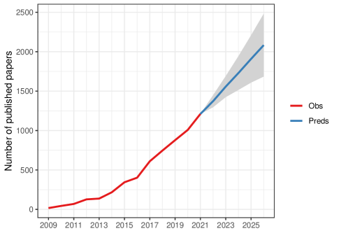
Citizen science (CS) and crowdsourcing involve volunteers and amateur scientists in the scientific process. Over the last decade the number of publications using CS data has increased dramatically (Fig 1). CS projects are now entrenched in many fields of science, including the notification and classification of astronomical events to learn about our universe, the identification and monitoring of environmental phenomena to learn about our world, and the reporting and assessment of health and medical outcomes to learn about our own selves. Quantitative information obtained from citizen scientists can be analysed in its own right, or it can fill gaps in professional data collection programs or experimental studies, or it can be used for complementary purposes such as training machine learning algorithms [11].
In the field of ecology, millions of citizen scientists are engaged in research projects worldwide, producing volumes of information in a cost-effective and timely manner and contributing substantively to aspirational targets such as the United Nations Sustainable Development Goals [46, 34]. These projects embrace a wide range of challenges, including assessments of climate change impacts, water and air quality measurements, monitoring of biodiversity trends and patterns in abundance, distribution, and richness of native and exotic species. Citizen science platforms have also become established. For example, iNaturalist, eButterfly and Zooniverse host hundreds of projects involving image classification. These online platforms have gained substantial recognition in recent years because they have the potential to reduce the workload of ecological experts and they engage large communities of contributors.
Notwithstanding the popularity and benefits of CS, considerable data quality concerns remain regarding research involving data elicited by non-expert citizen scientists [24]. These concerns primarily focus on the potential for bias arising from the unstructured nature of the data and the differing abilities of the participants. For example, while the individual classification accuracy is high in some CS image classification projects, ranging from 70% to 95% [e.g. 55], aggregation via some form of consensus is often required to produce reliable classifications and estimates [94, 93]. Many aggregation methods, including majority voting, enjoy great success in the literature. These methods rely on the assumption that participants have greater than 50% chance of answering correctly. However, such an assumption is not always satisfied in the presence of difficult tasks, in which the majority of the classifications can be incorrect [83].
In this paper, we focus on a particular set of problems that are of great interest for citizen science in ecology, namely the classification of objects in photos and videos. We investigate the feasibility of crowdsourcing methods for citizen science as a viable solution for manual classification of images when the task is difficult. This may occur, for example, if the images represent complex ecosystems, depicting aggregations of diverse species communities that change in space and time. Difficult tasks can also be related to images produced by different sources, such as environmental monitoring programs and cameras.
We consider this problem through a Bayesian lens. To set the work in context, we first present a scan of papers that have employed Bayesian models with citizen science in ecology. The 84 exemplar papers are summarised with respect to the aim of the study, the statistical model/method and software employed, the data captured and the platform enlisted. Of particular interest is the acknowledgement and treatment of potential bias in the CS data. We then study how a suitable statistical model based on item response theory (IRT) can improve the quality of crowdsourced information and enable it to be used more confidently to help answer relevant ecological problems and estimate complex measures such as ecosystem health. This model can be used to assess changes in participants’ abilities over time and whether they learn with more classification opportunities. It can also be used to identify those categories that are harder to classify and factors affecting the difficulties of the images.
Following discussion of the model, we present a case study of the classification of underwater images from the Great Barrier Reef (GBR), Australia. In the experiment, we showed coral reef images to non-expert participants and asked them to classify five broad categories of benthic communities using the Amazon Mechanical Turk platform (MTurk). The statistical approach developed in this paper allows us to estimate the most difficult benthic categories, investigate different types of difficulty, including those related to images and cameras, and detect different groups of participants, based on their abilities to perform the required tasks. We also examine the relationship between the time that a participant needed to perform the classification and the participants’ latent abilities.
The rest of the paper is structured as follows. A review of Bayesian methods for citizen science is provided in Section 2 followed by the introduction of a Bayesian item response model which addresses biases in image classification in Section 3. Section 4 details the paper’s case study in the Great Barrier Reef, Australia, including a results section summarising the applied models. Finally, Section 5 contains a detailed discussion centred around the quality of citizen science data for image classification specifically and for use in ecological research. It should be noted that we focus on images in this paper and often refer to images as ‘items’. Additionally, we use the term ‘label’ to refer to the true underlying category of the target observation in any reference images. Despite dealing with the classification of images in this study, the proposed methodology can be extrapolated to other sources of citizen science-produced data such as audio recordings.
2 Bayesian methods for citizen science
Scientists are increasingly employing Bayesian statistical methods to overcome some of the limitations of CS data. We conducted a scan of some of the most relevant developments, following the PRISMA guidelines (Preferred Reporting Items for Systematic Reviews and Meta-Analyses) [69]. We searched the Web of Science, Scopus, and Google Scholar databases using the keywords “citizen science” and “Bayes”, and filtered articles belonging to Ecology and Conservation. The search was restricted to articles in the English language published in peer-reviewed articles from 2010 to 30-Apr-2022.
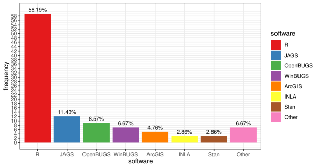
We found a total of 84 articles meeting the inclusion criteria. For each article, we summarised the statistical method used, the most relevant findings, the data sources, the platform/project and the software/packages used for modelling (if it was mentioned explicitly). The articles are summarized in Table LABEL:table:summ. In total, 36.4% of the articles used Bayesian regression and/or hierarchical models. A comparable percentage employed Bayesian species distribution models / Bayesian occupancy models. Approximately 20% of the models incorporate spatial and spatio-temporal dependence. Other statistical models not included in these categories accounted for 18%. In Fig 10 we have summarized the software used for Bayesian computation. Over half of the articles that specified the use of software mentioned the use of R [82], frequently in conjunction with dedicated software such as WinBUGS [62], OpenBUGS [102], Stan [12] and INLA [91]. Among the scanned paper, the most popular R packages for Bayesian inference are R2jags [110], rjags [80], R2OpenBUGS[109], rstan [103], unmarked [32], adegenet [51], ape[74], jagsUI [54], R2WinBUGS [109], rstanarm [39].
A substantial proportion of the scanned articles deals with topics such as the estimation of the presence/absence of species or their abundance. Hence, many authors resort to Bayesian occupancy and species distribution models [e.g. 21, 96, 16, 114, 27, 86]. Ecological data is generally geo-referenced and many of the models account for spatial variation by using for instance conditional autoregressive models (CAR) [4, 19, 25, 81, 94], covariance matrices [85], Gaussian processes [98], SPDE [35, 49] or simply incorporating spatially varying covariates.
One of our main aims was to explore the treatment authors give to CS-produced data. We found that researchers often assume that no errors or biases are present in the data, which could affect statistical inference and decision making. For example, many CS projects in ecology use opportunistic data that are obtained without a sampling design or a professional survey, since traditional professional programs are costly and time-consuming and can fail to obtain accurate or precise estimates of infrequent species or other outcomes of interest. Geographical, spatial recording, and preferential sampling bias may arise from opportunistically collected data, with more observations from frequently visited locations such as around roads, with irregular frequencies across time, or as a result of preferential sampling spots with certain habitat types or where specific species are more likely to be found. See the discussion in Chevalier et al. [15], Fournier et al. [33], Zhu et al. [125]. In addition, observer bias may arise as the result of inexperience, or incorrect understanding or perception of a variable of interest. Detection bias may arise if a species or outcome of interest is missed or misidentified.
Overall, we identified several strategies that have been proposed to cope with potential bias in CS data. A discussion around the use of opportunistic data can be found in Coron et al. [17]. Similarly, the temporal bias (observation efforts) arising from the seasonality of visitors to the area of study is addressed by Dwyer et al. [25], specifically for sightings data. In a spatial context, van Strien et al. [107] suggested using post-stratification of sites and showed how opportunistic data can produce suitable estimates when adjusting for bias produced by geographical imbalance and unequal observation efforts. In another study, Humphreys et al. [49] included human population density to account for the fact that sightings might be more likely in areas with larger populations. These authors also tackled observer bias by using observation effort expressed as observer hours as a predictor in their models.
Imperfect detection is relevant, especially for data contributed by citizen scientists. Occupancy models generally involve a component for the presence/absence and another for the detection/non-detection. These models aim at minimizing the misclassification rate (number of false negatives and false positives). Variations of this models can be found in Strebel et al. [105], Isaac et al. [50], Petracca et al. [79] and van Strien et al. [106]. See Isaac et al. [50] for a comparison of several Bayesian occupancy models in terms of the efficiency to detect trends based on different opportunistic data collection scenarios. Detection bias is also considered in Berberich et al. [10] by accounting for false-positive detection (specificity) bias when spotting red wood ant nests. Viljugrein et al. [116] also considered diagnostic sensitivity for the probability that an infected animal will be detected by testing. Similarly, Cumming and Henry [20] corrected for observation effort to account for imperfect detection. More recently, Eisma et al. [26] suggested a measurement error model to adjust for biases and errors in reports of rainfall measurement data produced by volunteers in Nepal.
There exists a fundamental gap in the literature regarding approaches to overcome other sources of bias. This includes potential biases resulting from the misclassification errors arising during the classification of objects on images by citizen scientists. We discuss this issue in the next section.
3 Addressing citizen science bias in image classification
In this section, we first discuss majority voting algorithms that are frequently used to estimate the true labels in manual image classification. This is followed by the introduction of a Bayesian item response model that is used to weight the evidence produced by citizen scientists.
3.1 Majority vote (MV)
We consider a set of images , each composed of elicitation points selected using a spatially balanced random sampling approach. We deal with a binary classification task, in which a participant is asked whether a category (e.g., coral) is present on a point belonging to a given image. Let be the answer of the participant for the point from the image.
| (1) |
By design, multiple participants classify the same point . Based on these answers, we obtain the majority vote by aggregating the answers, so that the category with the highest proportion of votes wins the vote, which is the mode.
| (2) |
In general, this approach performs poorly for difficult tasks. This is because only expert participants are likely to respond correctly, and they can be outvoted by beginners [83]. A variation of this method is obtained using a weighted majority voting (WMV) which has been discussed, among others, by Littlestone et al. [58], Lintott et al. [57], Hines et al. [44]. In this method, each participant has a vote proportional to some weights, based on their knowledge, skills or past performance.
3.2 Bayesian IRT model
The estimation of participants’ abilities in crowdsourced data has been widely discussed in the literature [121, 120, 76]. We develop a Bayesian item response model with the aim of informing a weighted consensus voting approach. Reiterating for completeness the notation introduced earlier, let the binary response variable represent whether a question associated with the point () on the image () taken using the camera is correctly answered or not by the participant (). We assume that follows a Bernoulli distribution with parameter
| (3) |
We use an extension of the item response model, namely the linear logistic test model (LLTM), which is formulated as follows
| (4) |
where and are difficulties associated with the point and the camera. The parameter represents the ability of the participant. The ability of an average participant can be anchored by setting it equal to zero to avoid identifiability issues with the model. Additionally, gives the slope of the logistic curve and is a pseudo-guessing associated with the point, indicating the probability of answering correctly due to guessing. We use Bayesian inference and therefore we need to define prior distributions for the parameters of interest in Eq4.
| # hierarchical prior on the abilities | ||||
| # flat prior on a weakly informative range for the s.d. of the users’ abilities | ||||
| # hierarchical prior on the item difficulties | ||||
| # weakly informative prior for the mean of the item difficulties | ||||
| # informative prior for the sd of the item difficulty, allowing for substantially complex tasks | ||||
| # hierarchical prior on the camera difficulties | ||||
| # weakly informative prior for the mean of camera difficulty | ||||
| # informative prior for the sd of the camera difficulties | ||||
| # normal prior with mean 1 on the slope | ||||
| # half Cauchy prior on the slope sd truncated at 0 | ||||
| # weakly informative prior on the pseudoguessing |
Changes in ability
Several authors have suggested the implementation of dynamic item response models that account for temporal variation in the answers, under the principle that subjects’ abilities change with time as a learning curve [e.g. 119]. To capture the learning in the process, we incorporated a temporally dependent component to the model
| (5) |
where is a common learning measure that captures the change in abilities according to the daily occasions that participants performed classifications . For participant , represents the first classification day, the second, and so on.
Consensus based on a Bayesian item response model
The model described above is set in the context of a broader workflow, described as follows:
-
1.
Produce a representative set of gold standard images e.g. 33% of the total number of images. In this set of images the true labels or answers will be obtained from expert elicitation or other another suitable method. Images in this set will be scored by most of the participants.
-
2.
Fit an item response model and obtain estimates of the participants’ abilities accounting for difficulties, guessing, etc.
-
3.
For a weighted consensus, derive a weight for each participant proportional to their estimated ability using the posterior mean. We can compute the weights using . Alternatively, a fully Bayesian framework can be employed by using the draws from the posterior distribution of to compute the distribution of .
-
4.
Perform a weighted consensus vote to estimate the labels. Since our response variable is binary, the category with the largest wins the weighted vote.
4 Case study: Classification of images from coral reefs
“How inappropriate to call this planet Earth when it is quite clearly Ocean.” - Arthur C. Clarke
The Great Barrier Reef (GBR) is located on Australia’s north eastern coast and is among the largest and most complex ecosystems in the world [41]. Two impacts of climate change, including the increasing frequency of reef bleaching events and intensity of cyclones, are negatively affecting this ecosystem causing an unprecedented decline in the prevalence of hard corals [47, 23, 1, 115]. Estimation and assessment of this decline are difficult and expensive to quantify using traditional marine surveys considering the size of the GBR and the speed of decline [37]. For this reason, some researchers are harnessing the strength of citizen science to produce estimates of reef-health indicators across large spatial and temporal scales [78, 94]. For instance, Santos Fernandez et al. [94], utilized a spatial misclassification model, taking into account the proficiency of the participant in terms of sensitivity and specificity to account for bias in the data. Information from these models can then be used by reef managers and scientists to make data-enabled management decisions and inform future research.
We performed an experiment using Amazon Mechanical Turk (https://www.mturk.com/) to assess the feasibility of using crowdsourced data for the estimation of hard coral cover, represented as the two-dimensional proportion of the seafloor covered in hard corals. Hard corals play an important role in reef ecosystems; their hard skeletons provide habitat for many organisms and they are vulnerable to a range of impacts that accumulate with climate change [47]. The dataset used in the study consisted of 514 geotagged images obtained from the XL Catlin Seaview Survey [38] and the University of Queensland’s Remote Sensing Research Centre [87], which we used to assess the participants’ abilities to identify hard corals. In practice, coral cover estimates from images are often based on a subset of classification points, rather than the whole image [113, 111]. In these two programs, 40 to 50 spatially balanced, random classification points were selected on each image and classified by coral reef scientists [37, 88]. We consider the classifications from the reef scientists as a gold standard (i.e. the ground truth).
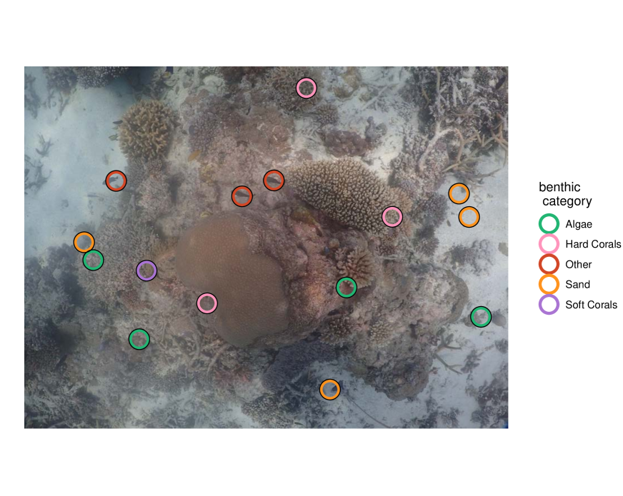
We engaged participants and provided instructions in an 11-page training document https://github.com/EdgarSantos-Fernandez/reef_misclassification/HelpGuide_MTurk20200203.pdf, describing how to identify the different benthic categories, which included: hard and soft corals, algae, sand, water and other. Participants were also given the option to select unsure if they were uncertain about which category to select. Several image classification examples were included in this guide and the differences between commonly misclassified benthic groups were highlighted https://www.virtualreef.org.au/wp-content/uploads/VirtualReefDiver-Classification-HelpGuide-Part2.pdf.
After studying the training document, a qualification task was used to assess the proficiency of the participants to accurately complete the task. More specifically, the participants were shown five images containing one classification point each and asked to select the correct class from the five possible choices. The qualification was granted to those scoring at least three correct classifications out of five.
We designed a sampling protocol to select images representative of the GBR in terms of community composition (proportion of hard and soft corals, algae, and sand) and camera types (Canon, Lumix, Olympus, Sony, and Nikon). This produced a dataset composed of 514 images. We produced 514 human intelligence tasks (HITS) with a maximum number of 70 assignments per HIT (i.e. maximum number of times each image can be classified).
Images were randomly assigned to the participants. We were concerned that classifying 40 or 50 points per image was too time consuming and that it would reduce participation. In addition, previous research has shown that accurate estimates of coral cover can be obtained with approximately 10 points Beijbom et al. [8]. Therefore, we asked participants to classify 15 classification points on each image, randomly selected from the 40-50 points previously classified by reef scientists. See the example in Fig.2. Participants were required to select a classification category for all of the points before submitting the classification. Every assignment (i.e. an image) was expected to take approximately one minute to complete. The payment was set to 0.10 USD per image and participants reported earning more than the federal minimum wage in the United States ($7.25 per hour) for their contributions. We monitored the quality of the classifications to prevent low-quality participants from contributing.
4.1 Performance measures
Our category of interest in the analyses is hard corals. We used a suite of performance measures to describe the ability of the participants, which are based on the true positive (TP), true negative (TN), false positive (FP), and false negative (FN). In this context, TP are the points classified as hard coral given that the point is truly occupied by hard corals. A TN occurs when the point is correctly classified as something other than hard coral when there is no hard coral present. Similarly, FP represents points classified as hard coral when hard coral is absent, while FN occurs when hard coral is incorrectly classified as something else. This information was then used to generate other performance measures such as:
-
•
Sensitivity: measures the ability of a participant to identify a category when it is present: .
-
•
Specificity: measures the ability of a participant to correctly identify a category when it is absent: .
-
•
Classification accuracy: the proportion of correctly identified classification points: .
-
•
Precision: the probability of correctly classifying points that truly contain the category hard coral divided by the total number of points classified as containing it .
-
•
Matthews correlation coefficient (MCC) [67]: a measure of the effectiveness of the classifier using all the elements of the confusion matrix.
-
•
positive likelihood ratio (): gives the number of true positives for every false positive.
-
•
negative likelihood ratio (): measures the number of false negatives for every true negative.
We fitted the Bayesian item response model given in Eq 5. We extracted the posterior distribution of the abilities () and clustered subjects. We then used these clusters to construct several model variations based on majority voting, restricted to experts or experts/experienced subjects. Three replicates were generated for different gold standard proportions and the results were averaged out.
4.2 Results
The data contributed by participants were aggregated using the five different methods. First, we considered the raw estimates obtained directly from the participants’ classifications (i.e. raw), without any grouping or consensus applied (Table 1). The columns in this table represent the number of classification points () and the performance measures.
We considered a traditional consensus and weighted variation based on item response model from Eq.5. The robustness of the results were assessed for the proposed consensus method using different proportions of images where the truth was known (10%, 20%, 33% and 50%); noting that images were randomly selected without replacement.
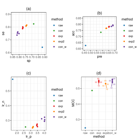
Using the raw data without combining the subjects’ answers produced relatively low-quality performance compared to other aggregation methods, and with an accuracy of 0.626 and . On average, the subjects identified 1.682 TP hard coral points for every FP hard coral classification. Using a traditional consensus approach combining all of the participants’ responses substantially increased the performance measures compared to the raw data method e.g. and .
The majority voting methods using a selection of the participants outperform () in all the variants explored. The ratio of TP/FP points identified under these methods is above 3. However, the likelihood ratio (FN/TN) was similar to the one obtained using the consensus approach. Fig 9 compares the statistical performance measures. In the case of the MV methods, we show four values per method representing the proportion of images in the gold standard set (10, 20, 33 and 50%). The last method (weighted variation) performed well compared to the approach based on experts and experienced, achieving marginal improvements in and . We found that the item response model captures well the abilities of the subjects, even with a small training dataset. This indicates that a minimal training set (e.g. 50 images) is enough to cluster subjects based on proficiency (i.e. expert, experienced, etc.).
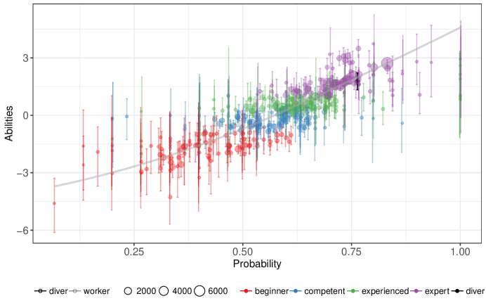
Four groups of participants were obtained from the quantiles of the posterior means of the abilities (Figure 3): beginners, competent, experienced and experts. The vertical axis gives the latent ability score () and the x-axis the proportion of correctly classified points. Skilful participants have large ability score values. The size of the point gives the number of classification points and indicates the engagement in the project. The vertical bar is the 95% posterior highest density interval and represents the dispersion around the posterior ability estimate. In black, we represent a reference participant who self-identified with diving experience. This participant falls within the expert category, yet remarkably it was not the best-performing one.
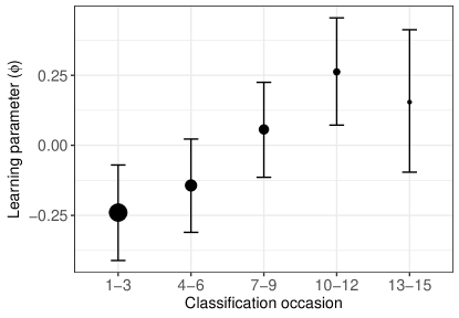
In Fig 4 we assess the dynamics of the rate of learning as the participants increased daily classification occasions (i.e. they work on the task a second, third, fourth time, etc). Fitting a linear regression to the posterior means at the occasion produced a slope significantly different from 0 (p-value = 0.019), which indicates that the participants’ skills increase with participation and they become better at classifying the points. After controlling for pseudo-guessing and discrimination, the average participant increased their probability of correct classification by approximately 4% after five occasions, and 8% and 12% in the and occasions, respectively.
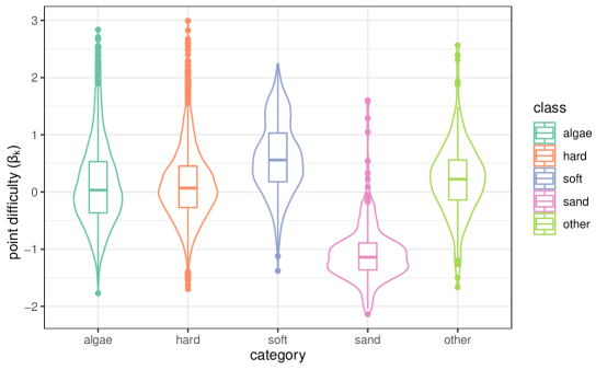
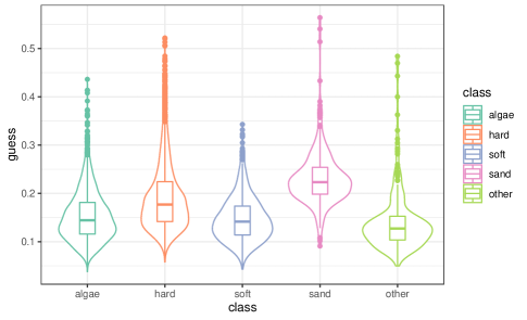
There were also differences in the difficulty of classifying each of the classes (Fig 5). The results showed that the soft coral category was the hardest to identify in the images since they are frequently misclassified as hard corals. As expected, points containing sand had the highest chances of correct classification. This category also exhibited the highest likelihood of being correctly identified by chance, as evidenced by the posterior distribution of the pseudo-guessing parameter (Fig 6).
.
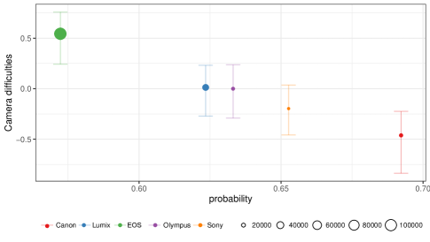
Substantial differences were found among the cameras used to take the images. Images taken by the Nikon camera represented the vast majority and they were substantially more difficult (Fig 7). This camera was used to take images in the northern section of the GBR on a unique habitat as part of the XL Catlin Seaview survey [38]. Images from the Canon camera, taken as part of the Heron survey across different habitats, were easier to classify [89]. However, the difficulty associated with the camera might be confounded by the regions where images were taken (North versus South of the GBR and habitats), where biodiversity differs.
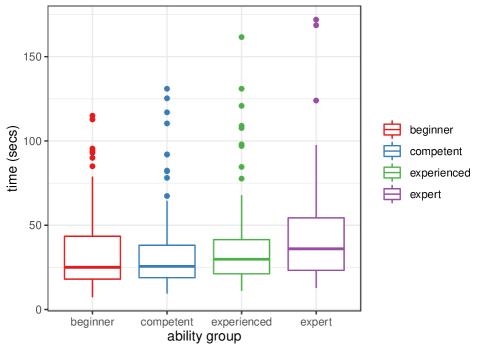
4.2.1 Classification time and quality
We evaluated the feasibility of using classification time as a straightforward indicator of classification quality. This is relevant in the context where participants are getting paid for completed images and thus trying to maximize their effort and it could be used as a straightforward way of detecting low-performing respondents.
The boxplots in Fig 8 show the distributions of the classification times for each of the participant groups. We note that those participants identified as expert seem to require significantly higher median classification times compared to those in the beginner and competent groups as shown in Table 2. The comparison was made using the non-parametric Wilcoxon test, with an alternative hypothesis that the sampled elements from the group in the rows had substantially greater mean rank values than those in the columns (Table 2). However, due to the substantial overlap between these distributions and variability in the data, these results should be interpreted with caution.
5 Discussion
5.1 Improving trust in citizen science data
Citizen science (CS) has become an essential information source in many domains. However, the validity of research outputs using these data sources is often questioned, especially when participants with varying skills are involved in challenging tasks. The lack of trust in this new type of data hampers the full potential of CS programs to support management and data-driven decision-making. Our scan of recently published papers highlighted the broad use of CS data in addressing ecological questions such as mapping species abundance and understanding their associated drivers through time. Some, but not all, of the studies recognized the potential inherent bias in CS data, acknowledging its ecological implications and adapting methodological approaches accordingly. Notwithstanding these efforts, further work is required to advance current statistical practice with CS data.
5.2 Improving trust in citizen science data for image classification
Our case study focused on the classification of objects in images and described a method that weights the evidence to produce the true latent labels, which are used to predict the health of coral populations along the Great Barrier Reef, Australia. This was achieved via estimation of participants’ abilities after accounting for factors such as image difficulty.
Applications based on image-based classification data are drawing increasing attention in many domains. It is therefore natural that there will be further opportunities to learn from the contribution of participants. However, new statistical methods are required if these opportunities are to be meaningfully realised. For example, the identification of benthic categories on images is currently deemed to be too challenging for most citizen scientists, who have little knowledge of what a hard coral looks like. Similarly, not all participants have the same commitment and skills and they engage differently in CS programs. This is critical when dealing with CS data and statistical models need to weigh the evidence, based on these factors.
Obtaining the true classes using marine biologists or expert elicitation is expensive when large numbers of images need to be classified. Our results show that an item response model is a viable option when there are budget constraints. The item response modelling framework provides an effective way to assess participants’ skills and cluster/group them by the level of expertise. This approach allows flexibility for the CS programs to select data and perform various assessments along the way [93]. For example, our case study demonstrates increasing learning of the participants with time. This insight showcases the importance of retention in CS programs as people naturally learn, even with complicated tasks. These models also allowed us to identify careless or low-skilled respondents and detect software bots, who generally fall into the beginners’ category. Responses from these participants are generally messy; therefore our voting algorithm does not include them. In our experience, this step was critical to achieving good classification performance.
We also showed that multiple factors affect the difficulty of the task, including the underlying category on the images and the camera type. Identifying those categories and images that produce greater misclassification errors is critical to producing useful training and qualification materials. Identifying and combining expert responses is a suitable solution and this can be done even with a reduced gold standard dataset.
Citizen science project managers can benefit from the approach in many ways: (1) Clustering participants allows weighting the evidence; (2) the ability to identify beginners means that they can be asked to re-qualify before contributing additional data; (3) gamification, such as leaderboards, can be constructed using the latent ability values and the number of classifications; and (4) a priori knowledge about which images are the most difficult could be used to assign them to the most skillful participants.
Currently, paid platforms such as Amazon Mechanical Turk do not consider the contribution of the participants or their expertise. Instead, whoever requests the job can refuse payment for poor-quality work. A system based on ability scores, as developed in this research, constitutes a better approach to compensate participants and is more effective than the current binary system. We found that for easy classification tasks, with broad evenness in the responses of the participants, most approaches will perform relatively well. However, when the task is difficult, aggregating the answers of the participants using simple consensus tends to have poor performance. Using instead a weighted majority voting approach improves performance outcomes.
5.3 Improving trust in citizen science data for ecology
The literature scan showed that most existing applications involve land-based ecosystem datasets. A substantial gap exists in the use of CS for marine ecology, especially in coral reef studies. Reef CS programs mostly exist to empower people and increase awareness, but few of them engage with robust and regular assessments of data quality which, in turn, reduce the trust of scientists and managers in using information collected by non-experts. However, marine research is evolving and collaborative CS programs such as Virtual Reef Diver combines modern statistical modelling and coral reef ecology to improve the integrity of CS data for decision-making. These methods can help marine ecology realise its full potential and contribute preservation of the health of the Great Barrier Reef by harnessing the strong engagement of several groups, including the online community. The valuable feedback we received in the study allowed us to improve project design, training, and compensation processes. An important feedback loop is also closed when measures of performance from the model are shared with the participants.
Guidelines when analysing new data sources such as CS data are essential to increase the trust among the scientific community. Our study focuses on Bayesian methods to analyse CS data, we acknowledge that other quantitative approaches not considered here, especially from the general crowdsourcing literature, can also add important value to CS projects. The item response model or similar statistical techniques should be systematically applied to first quantify and assess the quality of CS data and second support choices of a further analytical framework for ecological purposes. For example, insights from the model can be combined into species distribution models to weight observations according to participant skills or other parameters of interest before estimations of occupancy probability.
Data availability statement
The dataset used in the case study can be found in the repository: https://github.com/EdgarSantos-Fernandez/reef.
Acknowledgement
This research was supported by the Australian Research Council (ARC) Laureate Fellowship Program under the project “Bayesian Learning for Decision Making in the Big Data Era” (ID: FL150100150) and the Centre of Excellence for Mathematical and Statistical Frontiers (ACEMS). We thank the editor and the reviewers for their valuable feedback and constructive suggestions. Thanks to the members of the VRD team (https://www.virtualreef.org.au/about/). We also like to thank all the participants who contributed to the classification of images. Ethical approval was granted for the collection of this data by the Research Ethics Advisory Team, Queensland University of Technology (QUT). Approval Number: 1600000830. Computations were performed through the QUT High Performance Computing (HPC) infrastructure.
References
- Ainsworth et al. [2016] Ainsworth, T. D., Heron, S. F., Ortiz, J. C., Mumby, P. J., Grech, A., Ogawa, D., Eakin, C. M. and Leggat, W. (2016) Climate change disables coral bleaching protection on the Great Barrier Reef. Science, 352, 338–342.
- Allen et al. [2020] Allen, M. L., Wang, S., Olson, L. O., Li, Q. and Krofel, M. (2020) Counting cats for conservation: seasonal estimates of leopard density and drivers of distribution in the serengeti. Biodiversity and Conservation, 29, 3591–3608.
- Arab and Courter [2015] Arab, A. and Courter, J. R. (2015) Spatio-temporal trend analysis of spring arrival data for migratory birds. Communications in Statistics-Simulation and Computation, 44, 2535–2547.
- Arab et al. [2016] Arab, A., Courter, J. R. and Zelt, J. (2016) A spatio-temporal comparison of avian migration phenology using citizen science data. Spatial Statistics, 18, 234–245.
- Armstrong [2016] Armstrong, D. P. (2016) Using reference sites to account for detection probability in occupancy surveys for freshwater turtles. Herpetological Conservation and Biology, 11, 505–518.
- Barnes et al. [2015] Barnes, M., Szabo, J. K., Morris, W. K. and Possingham, H. (2015) Evaluating protected area effectiveness using bird lists in the australian wet tropics. Diversity and Distributions, 21, 368–378.
- Beck et al. [2014] Beck, S., Foote, A. D., Koetter, S., Harries, O., Mandleberg, L., Stevick, P. T., Whooley, P. and Durban, J. W. (2014) Using opportunistic photo-identifications to detect a population decline of killer whales (orcinus orca) in british and irish waters. Journal of the Marine Biological Association of the United Kingdom, 94, 1327–1333.
- Beijbom et al. [2015] Beijbom, O., Edmunds, P. J., Roelfsema, C., Smith, J., Kline, D. I., Neal, B. P., Dunlap, M. J., Moriarty, V., Fan, T.-Y., Tan, C.-J. et al. (2015) Towards automated annotation of benthic survey images: Variability of human experts and operational modes of automation. PloS one, 10, e0130312.
- Benshemesh et al. [2020] Benshemesh, J., Southwell, D., Barker, R. and McCarthy, M. (2020) Citizen scientists reveal nationwide trends and drivers in the breeding activity of a threatened bird, the Malleefowl (Leipoa Ocellata). Biological Conservation, 246, 108573.
- Berberich et al. [2016] Berberich, G. M., Dormann, C. F., Klimetzek, D., Berberich, M. B., Sanders, N. J. and Ellison, A. M. (2016) Detection probabilities for sessile organisms. Ecosphere, 7, e01546.
- Bradter et al. [2018] Bradter, U., Mair, L., Jönsson, M., Knape, J., Singer, A. and Snäll, T. (2018) Can opportunistically collected citizen science data fill a data gap for habitat suitability models of less common species? Methods in Ecology and Evolution, 9, 1667–1678.
- Carpenter et al. [2017] Carpenter, B., Gelman, A., Hoffman, M. D., Lee, D., Goodrich, B., Betancourt, M., Brubaker, M., Guo, J., Li, P. and Riddell, A. (2017) Stan: A probabilistic programming language. Journal of statistical software, 76.
- Chapman et al. [2015] Chapman, D. S., Bell, S., Helfer, S. and Roy, D. B. (2015) Unbiased inference of plant flowering phenology from biological recording data. Biological Journal of the Linnean Society, 115, 543–554.
- Cheney et al. [2013] Cheney, B., Thompson, P. M., Ingram, S. N., Hammond, P. S., Stevick, P. T., Durban, J. W., Culloch, R. M., Elwen, S. H., Mandleberg, L., Janik, V. M. et al. (2013) Integrating multiple data sources to assess the distribution and abundance of bottlenose dolphins t ursiops truncatus in scottish waters. Mammal Review, 43, 71–88.
- Chevalier et al. [2021] Chevalier, M., Broennimann, O., Cornuault, J. and Guisan, A. (2021) Data integration methods to account for spatial niche truncation effects in regional projections of species distribution. ECOLOGICAL APPLICATIONS, 31.
- Coomber et al. [2021] Coomber, F. G., Smith, B. R., August, T. A., Harrower, C. A., Powney, G. D. and Mathews, F. (2021) Using biological records to infer long-term occupancy trends of mammals in the UK. BIOLOGICAL CONSERVATION, 264.
- Coron et al. [2018] Coron, C., Calenge, C., Giraud, C. and Julliard, R. (2018) Bayesian estimation of species relative abundances and habitat preferences using opportunistic data. Environmental and ecological statistics, 25, 71–93.
- Crawford et al. [2020] Crawford, B. A., Olds, M. J., Maerz, J. C. and Moore, C. T. (2020) Estimating population persistence for at-risk species using citizen science data. Biological Conservation, 243, 108489.
- Croft et al. [2019] Croft, S., Ward, A. I., Aegerter, J. N. and Smith, G. C. (2019) Modeling current and potential distributions of mammal species using presence-only data: A case study on british deer. Ecology and Evolution, 9, 8724–8735.
- Cumming and Henry [2019] Cumming, G. S. and Henry, D. A. (2019) Point counts outperform line transects when sampling birds along routes in south african protected areas. African Zoology, 54, 187–198.
- Della Rocca and Milanesi [2022] Della Rocca, F. and Milanesi, P. (2022) The new dominator of the world: Modeling the global distribution of the japanese beetle under land use and climate change scenarios. LAND, 11.
- Dennis et al. [2017] Dennis, E. B., Morgan, B. J., Freeman, S. N., Ridout, M. S., Brereton, T. M., Fox, R., Powney, G. D. and Roy, D. B. (2017) Efficient occupancy model-fitting for extensive citizen-science data. PloS one, 12, e0174433.
- De’ath et al. [2012] De’ath, G., Fabricius, K. E., Sweatman, H. and Puotinen, M. (2012) The 27–year decline of coral cover on the Great Barrier Reef and its causes. Proceedings of the National Academy of Sciences, 109, 17995–17999.
- Downs et al. [2021] Downs, R. R., Ramapriyan, H. K., Peng, G. and Wei, Y. (2021) Perspectives on citizen science data quality. Frontiers in Climate, 3, 25.
- Dwyer et al. [2016] Dwyer, R. G., Carpenter-Bundhoo, L., Franklin, C. E. and Campbell, H. A. (2016) Using citizen-collected wildlife sightings to predict traffic strike hot spots for threatened species: a case study on the southern cassowary. Journal of Applied Ecology, 53, 973–982.
- Eisma et al. [2020] Eisma, J. A., Schoups, G., Davids, J. and Van de Giesen, N. (2020) A bayesian model for quantifying errors in citizen science data: application to rainfall observations from nepal.
- Erickson and Smith [2021] Erickson, K. D. and Smith, A. B. (2021) Accounting for imperfect detection in data from museums and herbaria when modeling species distributions: combining and contrasting data-level versus model-level bias correction. ECOGRAPHY, 44, 1341–1352.
- Eritja et al. [2017] Eritja, R., Palmer, J. R., Roiz, D., Sanpera-Calbet, I. and Bartumeus, F. (2017) Direct evidence of adult aedes albopictus dispersal by car. Scientific Reports, 7, 1–15.
- Espeset et al. [2016] Espeset, A. E., Harrison, J. G., Shapiro, A. M., Nice, C. C., Thorne, J. H., Waetjen, D. P., Fordyce, J. A. and Forister, M. L. (2016) Understanding a migratory species in a changing world: climatic effects and demographic declines in the Western Monarch revealed by four decades of intensive monitoring. OECOLOGIA, 181, 819–830.
- Farhadinia et al. [2018] Farhadinia, M. S., Moll, R. J., Montgomery, R. A., Ashrafi, S., Johnson, P. J., Hunter, L. T. and Macdonald, D. W. (2018) Citizen science data facilitate monitoring of rare large carnivores in remote montane landscapes. Ecological indicators, 94, 283–291.
- Faulkner et al. [2017] Faulkner, S. C., Verity, R., Roberts, D., Roy, S. S., Robertson, P. A., Stevenson, M. D. and Le Comber, S. C. (2017) Using geographic profiling to compare the value of sightings vs trap data in a biological invasion. Diversity and Distributions, 23, 104–112.
- Fiske and Chandler [2011] Fiske, I. and Chandler, R. (2011) unmarked: An R package for fitting hierarchical models of wildlife occurrence and abundance. Journal of Statistical Software, 43, 1–23. URL: https://www.jstatsoft.org/v43/i10/.
- Fournier et al. [2017] Fournier, A. M., Sullivan, A. R., Bump, J. K., Perkins, M., Shieldcastle, M. C. and King, S. L. (2017) Combining citizen science species distribution models and stable isotopes reveals migratory connectivity in the secretive virginia rail. Journal of Applied Ecology, 54, 618–627.
- Fritz et al. [2019] Fritz, S., See, L., Carlson, T., Haklay, M. M., Oliver, J. L., Fraisl, D., Mondardini, R., Brocklehurst, M., Shanley, L. A., Schade, S. et al. (2019) Citizen science and the United Nations Sustainable Development Goals. Nature Sustainability, 2, 922–930.
- Girardello et al. [2019] Girardello, M., Chapman, A., Dennis, R., Kaila, L., Borges, P. A. and Santangeli, A. (2019) Gaps in butterfly inventory data: A global analysis. Biological conservation, 236, 289–295.
- Gomez et al. [2021] Gomez, A. M., Serre, M., Wise, E. and Pavelsky, T. (2021) Integrating community science research and space-time mapping to determine depth to groundwater in a remote rural region. WATER RESOURCES RESEARCH, 57.
- Gonzalez-Rivero et al. [2020] Gonzalez-Rivero, M., Beijbom, O., Rodriguez-Ramirez, A., Bryant, D. E., Ganase, A., Gonzalez-Marrero, Y., Herrera-Reveles, A., Kennedy, E. V., Kim, C. J., Lopez-Marcano, S. et al. (2020) Monitoring of coral reefs using artificial intelligence: A feasible and cost-effective approach. Remote Sensing, 12, 489.
- González-Rivero et al. [2014] González-Rivero, M., Bongaerts, P., Beijbom, O., Pizarro, O., Friedman, A., Rodriguez-Ramirez, A., Upcroft, B., Laffoley, D., Kline, D., Bailhache, C. et al. (2014) The Catlin Seaview Survey–kilometre-scale seascape assessment, and monitoring of coral reef ecosystems. Aquatic Conservation: Marine and Freshwater Ecosystems, 24, 184–198.
- Goodrich et al. [2022] Goodrich, B., Gabry, J., Ali, I. and Brilleman, S. (2022) rstanarm: Bayesian applied regression modeling via Stan. URL: https://mc-stan.org/rstanarm/. R package version 2.21.3.
- Granroth-Wilding et al. [2017] Granroth-Wilding, H., Primmer, C., Lindqvist, M., Poutanen, J., Thalmann, O., Aspi, J., Harmoinen, J., Kojola, I. and Laaksonen, T. (2017) Non-invasive genetic monitoring involving citizen science enables reconstruction of current pack dynamics in a re-establishing wolf population. BMC ecology, 17, 44.
- Great Barrier Reef Marine Park Authority [2009] Great Barrier Reef Marine Park Authority (2009) Great barrier reef outlook report 2009: In brief. Great Barrier Reef Marine Park Authority.
- Hertzog et al. [2021] Hertzog, L. R., Frank, C., Klimek, S., Roeder, N., Boehner, H. G. S. and Kamp, J. (2021) Model-based integration of citizen science data from disparate sources increases the precision of bird population trends. DIVERSITY AND DISTRIBUTIONS, 27, 1106–1119.
- Hill and Lloyd [2017] Hill, J. M. and Lloyd, J. D. (2017) A fine-scale us population estimate of a montane spruce–fir bird species of conservation concern. Ecosphere, 8, e01921.
- Hines et al. [2015] Hines, G., Swanson, A., Kosmala, M. and Lintott, C. (2015) Aggregating user input in ecology citizen science projects. In Twenty-Seventh IAAI Conference.
- Hof et al. [2017] Hof, C. A., Smallwood, E., Meager, J. and Bell, I. P. (2017) First citizen-science population abundance and growth rate estimates for green sea turtles chelonia mydas foraging in the northern great barrier reef, australia. Marine Ecology Progress Series, 574, 181–191.
- Hsu et al. [2014] Hsu, A., Malik, O., Johnson, L. and Esty, D. C. (2014) Development: Mobilize citizens to track sustainability. Nature News, 508, 33.
- Hughes et al. [2017] Hughes, T. P., Barnes, M. L., Bellwood, D. R., Cinner, J. E., Cumming, G. S., Jackson, J. B., Kleypas, J., Van De Leemput, I. A., Lough, J. M., Morrison, T. H. et al. (2017) Coral reefs in the anthropocene. Nature, 546, 82–90.
- Hultquist et al. [2021] Hultquist, C., Oravecz, Z. and Cervone, G. (2021) A bayesian approach to estimate the spatial distribution of crowdsourced radiation measurements around fukushima. ISPRS INTERNATIONAL JOURNAL OF GEO-INFORMATION, 10.
- Humphreys et al. [2019] Humphreys, J. M., Murrow, J. L., Sullivan, J. D. and Prosser, D. J. (2019) Seasonal occurrence and abundance of dabbling ducks across the continental united states: Joint spatio-temporal modelling for the genus anas. Diversity and Distributions.
- Isaac et al. [2014] Isaac, N. J., van Strien, A. J., August, T. A., de Zeeuw, M. P. and Roy, D. B. (2014) Statistics for citizen science: extracting signals of change from noisy ecological data. Methods in Ecology and Evolution, 5, 1052–1060.
- Jombart and Ahmed [2011] Jombart, T. and Ahmed, I. (2011) adegenet 1.3-1: new tools for the analysis of genome-wide snp data. Bioinformatics.
- Kadoya and Washitani [2010] Kadoya, T. and Washitani, I. (2010) Predicting the rate of range expansion of an invasive alien bumblebee (Bombus Terrestris) using a stochastic spatio-temporal model. Biological Conservation, 143, 1228–1235.
- Kagawa et al. [2020] Kagawa, O., Uchida, S., Yamazaki, D., Osawa, Y., Ito, S. and Chiba, S. (2020) Citizen science via social media revealed conditions of symbiosis between a marine gastropod and an epibiotic alga. Scientific reports, 10, 1–10.
- Kellner [2021] Kellner, K. (2021) jagsUI: A Wrapper Around ’rjags’ to Streamline ’JAGS’ Analyses. URL: https://CRAN.R-project.org/package=jagsUI. R package version 1.5.2.
- Kosmala et al. [2016] Kosmala, M., Wiggins, A., Swanson, A. and Simmons, B. (2016) Assessing data quality in citizen science. Frontiers in Ecology and the Environment, 14, 551–560.
- Lavariega et al. [2020] Lavariega, M. C., Ríos-Solís, J. A., Flores-Martínez, J. J., Galindo-Aguilar, R. E., Sánchez-Cordero, V., Juan-Albino, S. and Soriano-Martínez, I. (2020) Community-based monitoring of jaguar (panthera onca) in the chinantla region, mexico. Tropical Conservation Science, 13, 1940082920917825.
- Lintott et al. [2008] Lintott, C. J., Schawinski, K., Slosar, A., Land, K., Bamford, S., Thomas, D., Raddick, M. J., Nichol, R. C., Szalay, A., Andreescu, D. et al. (2008) Galaxy zoo: morphologies derived from visual inspection of galaxies from the sloan digital sky survey. Monthly Notices of the Royal Astronomical Society, 389, 1179–1189.
- Littlestone et al. [1989] Littlestone, N., Warmuth, M. K. et al. (1989) The weighted majority algorithm. University of California, Santa Cruz, Computer Research Laboratory.
- Lopez et al. [2020] Lopez, B., Minor, E. and Crooks, A. (2020) Insights into human-wildlife interactions in cities from bird sightings recorded online. LANDSCAPE AND URBAN PLANNING, 196.
- Lottig et al. [2014] Lottig, N. R., Wagner, T., Henry, E. N., Cheruvelil, K. S., Webster, K. E., Downing, J. A. and Stow, C. A. (2014) Long-term citizen-collected data reveal geographical patterns and temporal trends in lake water clarity. PloS one, 9, e95769.
- Louvrier et al. [2020] Louvrier, J., Papaïx, J., Duchamp, C. and Gimenez, O. (2020) A mechanistic-statistical species distribution model to explain and forecast wolf (canis lupus) colonization in south-eastern france. Spatial Statistics, 100428.
- Lunn et al. [2000] Lunn, D. J., Thomas, A., Best, N. and Spiegelhalter, D. (2000) WinBUGS - A Bayesian modelling framework: concepts, structure, and extensibility. Statistics and computing, 10, 325–337.
- Lyon et al. [2019] Lyon, J. P., Bird, T. J., Kearns, J., Nicol, S., Tonkin, Z., Todd, C. R., O’Mahony, J., Hackett, G., Raymond, S., Lieschke, J. et al. (2019) Increased population size of fish in a lowland river following restoration of structural habitat. Ecological Applications, 29, e01882.
- Maguire and Mundle [2020] Maguire, T. J. and Mundle, S. O. (2020) Citizen science data show temperature-driven declines in riverine sentinel invertebrates. Environmental Science & Technology Letters, 7, 303–307.
- Mair et al. [2017] Mair, L., Harrison, P. J., Jönsson, M., Löbel, S., Nordén, J., Siitonen, J., Lämås, T., Lundström, A. and Snäll, T. (2017) Evaluating citizen science data for forecasting species responses to national forest management. Ecology and evolution, 7, 368–378.
- Mang et al. [2017] Mang, T., Essl, F., Moser, D., Karrer, G., Kleinbauer, I. and Dullinger, S. (2017) Accounting for imperfect observation and estimating true species distributions in modelling biological invasions. Ecography, 40, 1187–1197.
- Matthews [1975] Matthews, B. W. (1975) Comparison of the predicted and observed secondary structure of t4 phage lysozyme. Biochimica et Biophysica Acta (BBA)-Protein Structure, 405, 442–451.
- Meiman et al. [2012] Meiman, S., Civco, D., Holsinger, K. and Elphick, C. S. (2012) Comparing habitat models using ground-based and remote sensing data: Saltmarsh Sparrow presence versus nesting. Wetlands, 32, 725–736.
- Moher et al. [2009] Moher, D., Liberati, A., Tetzlaff, J., Altman, D. G., Group, P. et al. (2009) Preferred reporting items for systematic reviews and meta-analyses: the prisma statement. PLoS med, 6, e1000097.
- Morii et al. [2018] Morii, Y., Ohkubo, Y. and Watanabe, S. (2018) Activity of invasive slug limax maximus in relation to climate conditions based on citizen’s observations and novel regularization based statistical approaches. Science of the Total Environment, 637, 1061–1068.
- Mugford et al. [2021] Mugford, J., Moltchanova, E., Plank, M., Sullivan, J., Byrom, A. and James, A. (2021) Citizen science decisions: A Bayesian approach optimises effort. ECOLOGICAL INFORMATICS, 63.
- Outhwaite et al. [2019] Outhwaite, C. L., Powney, G. D., August, T. A., Chandler, R. E., Rorke, S., Pescott, O. L., Harvey, M., Roy, H. E., Fox, R., Roy, D. B. et al. (2019) Annual estimates of occupancy for bryophytes, lichens and invertebrates in the uk, 1970–2015. Scientific data, 6, 1–12.
- Pagel et al. [2014] Pagel, J., Anderson, B. J., O’Hara, R. B., Cramer, W., Fox, R., Jeltsch, F., Roy, D. B., Thomas, C. D. and Schurr, F. M. (2014) Quantifying range-wide variation in population trends from local abundance surveys and widespread opportunistic occurrence records. Methods in Ecology and Evolution, 5, 751–760.
- Paradis and Schliep [2019] Paradis, E. and Schliep, K. (2019) ape 5.0: an environment for modern phylogenetics and evolutionary analyses in R. Bioinformatics, 35, 526–528.
- Patten et al. [2019] Patten, M. A., Hjalmarson, E. A., Smith-Patten, B. D. and Bried, J. T. (2019) Breeding thresholds in opportunistic odonata records. Ecological Indicators, 106, 105460.
- Paun et al. [2018] Paun, S., Carpenter, B., Chamberlain, J., Hovy, D., Kruschwitz, U. and Poesio, M. (2018) Comparing bayesian models of annotation. Transactions of the Association for Computational Linguistics, 6, 571–585.
- Penone et al. [2013] Penone, C., Le Viol, I., Pellissier, V., JULIEN, J.-F., Bas, Y. and Kerbiriou, C. (2013) Use of large-scale acoustic monitoring to assess anthropogenic pressures on orthoptera communities. Conservation Biology, 27, 979–987.
- Peterson et al. [2020] Peterson, E. E., Santos-Fernández, E., Chen, C., Clifford, S., Vercelloni, J., Pearse, A., Brown, R., Christensen, B., James, A., Anthony, K. et al. (2020) Monitoring through many eyes: Integrating disparate datasets to improve monitoring of the great barrier reef. Environmental Modelling & Software, 124, 104557.
- Petracca et al. [2018] Petracca, L. S., Frair, J. L., Cohen, J. B., Calderón, A. P., Carazo-Salazar, J., Castañeda, F., Corrales-Gutiérrez, D., Foster, R. J., Harmsen, B., Hernández-Potosme, S. et al. (2018) Robust inference on large-scale species habitat use with interview data: The status of jaguars outside protected areas in central america. Journal of applied ecology, 55, 723–734.
- Plummer [2022] Plummer, M. (2022) rjags: Bayesian Graphical Models using MCMC. URL: https://CRAN.R-project.org/package=rjags. R package version 4-13.
- Purse et al. [2015] Purse, B. V., Comont, R., Butler, A., Brown, P. M., Kessel, C. and Roy, H. E. (2015) Landscape and climate determine patterns of spread for all colour morphs of the alien ladybird harmonia axyridis. Journal of Biogeography, 42, 575–588.
- R Core Team [2018] R Core Team (2018) R: A Language and Environment for Statistical Computing. R Foundation for Statistical Computing, Vienna, Austria. URL: https://www.R-project.org/.
- Raykar et al. [2010] Raykar, V. C., Yu, S., Zhao, L. H., Valadez, G. H., Florin, C., Bogoni, L. and Moy, L. (2010) Learning from crowds. Journal of Machine Learning Research, 11, 1297–1322.
- Régnier et al. [2021] Régnier, T., Dodd, J., Benjamins, S., Gibb, F. M. and Wright, P. J. (2021) Age and growth of the critically endangered flapper skate, Dipturus intermedius. Aquatic Conservation: Marine and Freshwater Ecosystems, 31, 2381–2388.
- Reich et al. [2018] Reich, B. J., Pacifici, K. and Stallings, J. W. (2018) Integrating auxiliary data in optimal spatial design for species distribution modelling. Methods in Ecology and Evolution, 9, 1626–1637.
- Rodhouse et al. [2021] Rodhouse, T. J., Rose, S., Hawkins, T. and Rodriguez, R. M. (2021) Audible bats provide opportunities for citizen scientists. Conservation Science and Practice, 3, e435.
- Roelfsema et al. [2018] Roelfsema, C., Kovacs, E., Ortiz, J. C., Wolff, N. H., Callaghan, D., Wettle, M., Ronan, M., Hamylton, S. M., Mumby, P. J. and Phinn, S. (2018) Coral reef habitat mapping: A combination of object-based image analysis and ecological modelling. Remote sensing of environment, 208, 27–41.
- Roelfsema et al. [2021] Roelfsema, C., Kovacs, E. M., Markey, K., Vercelloni, J., Rodriguez-Ramirez, A., Lopez-Marcano, S., Gonzalez-Rivero, M., Hoegh-Guldberg, O. and Phinn, S. R. (2021) Benthic and coral reef community field data for heron reef, southern great barrier reef, australia, 2002–2018. Scientific data, 8, 1–7.
- Roelfsema and Phinn [2010] Roelfsema, C. and Phinn, S. (2010) Calibration and validation of coral reef benthic community maps derived from high spatial resolution satellite imagery. Journal of Applied Remote Sensing, 4, 043527.
- Roth et al. [2014] Roth, T., Strebel, N. and Amrhein, V. (2014) Estimating unbiased phenological trends by adapting site-occupancy models. Ecology, 95, 2144–2154.
- Rue et al. [2009] Rue, H., Martino, S. and Chopin, N. (2009) Approximate bayesian inference for latent gaussian models by using integrated nested laplace approximations. Journal of the royal statistical society: Series b (statistical methodology), 71, 319–392.
- Ryan et al. [2019] Ryan, S. F., Lombaert, E., Espeset, A., Vila, R., Talavera, G., Dincă, V., Doellman, M. M., Renshaw, M. A., Eng, M. W., Hornett, E. A. et al. (2019) Global invasion history of the agricultural pest butterfly pieris rapae revealed with genomics and citizen science. Proceedings of the National Academy of Sciences, 116, 20015–20024.
- Santos-Fernandez and Mengersen [2021] Santos-Fernandez, E. and Mengersen, K. (2021) Understanding the reliability of citizen science observational data using item response models. Methods in Ecology and Evolution, 12, 1533–1548.
- Santos Fernandez et al. [2020] Santos Fernandez, E., Peterson, E. E., Vercelloni, J., Rushworth, E. and Mengersen, K. (2020) Correcting misclassification errors in crowdsourced ecological data: A bayesian perspective. Journal of the Royal Statistical Society: Series C (Applied Statistics), n/a. URL: https://rss.onlinelibrary.wiley.com/doi/abs/10.1111/rssc.12453.
- Schwoerer et al. [2022] Schwoerer, T., Dial, R. J., Little, J. M., Martin, A. E., Morton, J. M., Schmidt, I, J. and Ward, E. J. (2022) Flight plan for the future: floatplane pilots and researchers team up to predict invasive species dispersal in Alaska. BIOLOGICAL INVASIONS, 24, 1229–1245.
- Sheard et al. [2021] Sheard, J. K., Rahbek, C., Dunn, R. R., Sanders, N. J. and Isaac, N. J. (2021) Long-term trends in the occupancy of ants revealed through use of multi-sourced datasets. Biology Letters, 17, 20210240.
- Shima et al. [2018] Shima, A. L., Gillieson, D. S., Crowley, G. M., Dwyer, R. G. and Berger, L. (2018) Factors affecting the mortality of Lumholtz’s tree-kangaroo (Dendrolagus Lumholtzi) by vehicle strike. Wildlife Research, 45, 559–569.
- Sicacha-Parada et al. [2020] Sicacha-Parada, J., Steinsland, I., Cretois, B. and Borgelt, J. (2020) Accounting for spatial varying sampling effort due to accessibility in citizen science data: A case study of moose in norway. Spatial Statistics, 100446.
- Siddharthan et al. [2016] Siddharthan, A., Lambin, C., Robinson, A.-M., Sharma, N., Comont, R., O’mahony, E., Mellish, C. and Wal, R. V. D. (2016) Crowdsourcing without a crowd: Reliable online species identification using bayesian models to minimize crowd size. ACM Transactions on Intelligent Systems and Technology (TIST), 7, 45.
- Snäll et al. [2011] Snäll, T., Kindvall, O., Nilsson, J. and Pärt, T. (2011) Evaluating citizen-based presence data for bird monitoring. Biological conservation, 144, 804–810.
- Soykan et al. [2016] Soykan, C. U., Sauer, J., Schuetz, J. G., LeBaron, G. S., Dale, K. and Langham, G. M. (2016) Population trends for north american winter birds based on hierarchical models. Ecosphere, 7, e01351.
- Spiegelhalter et al. [2007] Spiegelhalter, D., Thomas, A., Best, N. and Lunn, D. (2007) Openbugs user manual. Version, 3, 2007.
- Stan Development Team [2018] Stan Development Team (2018) RStan: the R interface to Stan. URL: http://mc-stan.org/. R package version 2.18.2.
- Steger et al. [2017] Steger, C., Butt, B. and Hooten, M. B. (2017) Safari science: assessing the reliability of citizen science data for wildlife surveys. Journal of Applied Ecology, 54, 2053–2062.
- Strebel et al. [2014] Strebel, N., Kéry, M., Schaub, M. and Schmid, H. (2014) Studying phenology by flexible modelling of seasonal detectability peaks. Methods in Ecology and Evolution, 5, 483–490.
- van Strien et al. [2013a] van Strien, A. J., van Swaay, C. A. and Termaat, T. (2013a) Opportunistic citizen science data of animal species produce reliable estimates of distribution trends if analysed with occupancy models. Journal of Applied Ecology, 50, 1450–1458.
- van Strien et al. [2013b] van Strien, A. J., Termaat, T., Kalkman, V., Prins, M., De Knijf, G., Gourmand, A.-L., Houard, X., Nelson, B., Plate, C., Prentice, S. et al. (2013b) Occupancy modelling as a new approach to assess supranational trends using opportunistic data: a pilot study for the damselfly calopteryx splendens. Biodiversity and Conservation, 22, 673–686.
- Studds et al. [2021] Studds, C. E., Wunderle, Jr., J. M. and Marra, P. P. (2021) Strong differences in migratory connectivity patterns among species of Neotropical-Nearctic migratory birds revealed by combining stable isotopes and abundance in a Bayesian assignment analysis. JOURNAL OF BIOGEOGRAPHY, 48, 1746–1757.
- Sturtz et al. [2005] Sturtz, S., Ligges, U. and Gelman, A. (2005) R2winbugs: A package for running winbugs from r. Journal of Statistical Software, 12, 1–16. URL: http://www.jstatsoft.org.
- Su and Yajima [2021] Su, Y.-S. and Yajima, M. (2021) R2jags: Using R to Run JAGS. URL: https://CRAN.R-project.org/package=R2jags. R package version 0.7-1.
- Sweatman et al. [2005] Sweatman, H., Burgess, S., Cheal, A., Coleman, G., Delean, J. S. C., Emslie, M., Miller, I., Osborne, K., McDonald, A. and Thompson, A. (2005) Long-term monitoring of the great barrier reef.
- Szabo et al. [2010] Szabo, J. K., Vesk, P. A., Baxter, P. W. and Possingham, H. P. (2010) Regional avian species declines estimated from volunteer-collected long-term data using list length analysis. Ecological Applications, 20, 2157–2169.
- Thompson et al. [2016] Thompson, A., Costello, P., Davidson, J., Logan, M., Coleman, G., Gunn, K. and Schaffelke, B. (2016) Marine monitoring program: Annual report for inshore coral reef monitoring 2014-2015.
- Ver Hoef et al. [2021] Ver Hoef, J. M., Johnson, D., Angliss, R. and Higham, M. (2021) Species density models from opportunistic citizen science data. METHODS IN ECOLOGY AND EVOLUTION, 12, 1911–1925.
- Vercelloni et al. [2020] Vercelloni, J., Liquet, B., Kennedy, E. V., González-Rivero, M., Caley, M. J., Peterson, E. E., Puotinen, M., Hoegh-Guldberg, O. and Mengersen, K. (2020) Forecasting intensifying disturbance effects on coral reefs. Global change biology, 26, 2785–2797.
- Viljugrein et al. [2019] Viljugrein, H., Hopp, P., Benestad, S. L., Nilsen, E. B., Våge, J., Tavornpanich, S., Rolandsen, C. M., Strand, O. and Mysterud, A. (2019) A method that accounts for differential detectability in mixed samples of long-term infections with applications to the case of chronic wasting disease in cervids. Methods in Ecology and Evolution, 10, 134–145.
- Vincent et al. [2022] Vincent, J. G., Schuster, R., Wilson, S., Fink, D. and Bennett, J. R. (2022) Clustering community science data to infer songbird migratory connectivity in the western hemisphere. ECOSPHERE, 13.
- Walker and Taylor [2020] Walker, J. and Taylor, P. D. (2020) Evaluating the efficacy of eBird data for modeling historical population trajectories of North American birds and for monitoring populations of boreal and Arctic breeding species. AVIAN CONSERVATION AND ECOLOGY, 15.
- Wang et al. [2013] Wang, X., Berger, J. O., Burdick, D. S. et al. (2013) Bayesian analysis of dynamic item response models in educational testing. The Annals of Applied Statistics, 7, 126–153.
- Welinder and Perona [2010] Welinder, P. and Perona, P. (2010) Online crowdsourcing: rating annotators and obtaining cost-effective labels. In 2010 IEEE Computer Society Conference on Computer Vision and Pattern Recognition-Workshops, 25–32. IEEE.
- Whitehill et al. [2009] Whitehill, J., Wu, T.-f., Bergsma, J., Movellan, J. R. and Ruvolo, P. L. (2009) Whose vote should count more: Optimal integration of labels from labelers of unknown expertise. In Advances in neural information processing systems, 2035–2043.
- Wilson et al. [2013] Wilson, S., Anderson, E. M., Wilson, A. S., Bertram, D. F. and Arcese, P. (2013) Citizen science reveals an extensive shift in the winter distribution of migratory western grebes. PLoS One, 8, e65408.
- Yan et al. [2016] Yan, W., Hutchins, M., Loiselle, S. and Hall, C. (2016) An informatics approach for smart evaluation of water quality related ecosystem services. Annals of Data Science, 3, 251–264.
- Yoshikawa and Osada [2015] Yoshikawa, T. and Osada, Y. (2015) Dietary compositions and their seasonal shifts in japanese resident birds, estimated from the analysis of volunteer monitoring data. PloS one, 10, e0119324.
- Zhu et al. [2020] Zhu, Q., Hobson, K. A., Zhao, Q., Zhou, Y., Damba, I., Batbayar, N., Natsagdorj, T., Davaasuren, B., Antonov, A., Guan, J. et al. (2020) Migratory connectivity of swan geese based on species’ distribution models, feather stable isotope assignment and satellite tracking. Diversity and Distributions.
- Zipkin and Saunders [2018] Zipkin, E. F. and Saunders, S. P. (2018) Synthesizing multiple data types for biological conservation using integrated population models. Biological Conservation, 217, 240–250.
6 Tables
| method | n | TP | FP | TN | FN | |||||||
| raw | 614,160 | 132,752 | 155,482 | 251,849 | 74,077 | 0.642 | 0.618 | 0.626 | 0.461 | 0.246 | 1.682 | 0.579 |
| consensus | 23,488 | 6,779 | 4,798 | 10,470 | 1,441 | 0.825 | 0.686 | 0.734 | 0.586 | 0.487 | 2.624 | 0.256 |
| experts, GS:10%, | 23,488 | 6,468 | 3,468 | 11,794 | 1,750 | 0.787 | 0.773 | 0.778 | 0.652 | 0.541 | 3.480 | 0.275 |
| experts, GS:20%, | 23,488 | 6,520 | 3,510 | 11,752 | 1,699 | 0.793 | 0.770 | 0.778 | 0.650 | 0.543 | 3.451 | 0.268 |
| experts, GS:33%, | 23,488 | 6,541 | 3,513 | 11,747 | 1,677 | 0.796 | 0.770 | 0.779 | 0.651 | 0.545 | 3.457 | 0.265 |
| experts, GS:50%, | 23,488 | 6,588 | 3,495 | 11,767 | 1,632 | 0.801 | 0.771 | 0.782 | 0.653 | 0.552 | 3.500 | 0.258 |
| experts/experienced, GS:10%, | 23,488 | 6,637 | 3,883 | 11,385 | 1,583 | 0.807 | 0.746 | 0.767 | 0.631 | 0.531 | 3.186 | 0.258 |
| experts/experienced, GS:20%, | 23,488 | 6,665 | 3,906 | 11,362 | 1,555 | 0.811 | 0.744 | 0.767 | 0.631 | 0.532 | 3.174 | 0.254 |
| experts/experienced, GS:33%, | 23,488 | 6,704 | 3,969 | 11,299 | 1,516 | 0.816 | 0.740 | 0.766 | 0.628 | 0.532 | 3.137 | 0.249 |
| experts/experienced, GS:50%, | 23,488 | 6,675 | 3,925 | 11,343 | 1,545 | 0.812 | 0.743 | 0.767 | 0.630 | 0.532 | 3.160 | 0.253 |
| weighted, exp/exp,GS:10%, | 23,488 | 6,155 | 3,043 | 12,219 | 2,063 | 0.749 | 0.801 | 0.783 | 0.671 | 0.539 | 3.810 | 0.311 |
| weighted, exp/exp,GS:20%, | 23,488 | 6,057 | 2,806 | 12,456 | 2,162 | 0.737 | 0.816 | 0.788 | 0.684 | 0.545 | 4.023 | 0.322 |
| weighted, exp/exp,GS:33%, | 23,488 | 6,182 | 2,852 | 12,409 | 2,036 | 0.752 | 0.813 | 0.792 | 0.684 | 0.554 | 4.029 | 0.305 |
| weighted, exp/exp,GS:50%, | 23,488 | 6,262 | 2,898 | 12,364 | 1,957 | 0.762 | 0.810 | 0.793 | 0.684 | 0.559 | 4.013 | 0.294 |
| beginner | competent | experienced | |
|---|---|---|---|
| competent | 1.0000 | ||
| experienced | 0.5932 | 0.2955 | |
| expert | 0.0037 | 0.0009 | 0.0781 |
7 Supplementary Materials
Summary of Bayesian methods in Citizen Science
| Author(s) | Method | Description | Software / package | Data | Platform |
| Della Rocca and Milanesi [21] | Species distribution model | Assessing and predicting Japanese beetle species distributions to identify potential invasion locations | R(rinat, adehabitatHR, mclust, envirem) | International occurrence records for the Japanese beetle (2010-2020) | iNaturalist |
| Vincent et al. [117] | Connectivity analysis (Bayes’ rule) | Methodology for estimating patterns of migratory connectivity for songbirds using relative abundance models | R (adehabitat, NbClust, cluster) | Relative abundance estimates data for wood thrush and Wilson’s warbler songbirds (2016-2017, international) | eBird |
| Schwoerer et al. [95] | Bayesian hierarchical model | Using float-plane flight pathway data to inform early detection of aquatic invasive species | R (rstanarm) | Flight destination data (2015-2016, Alaska, North America) | |
| Santos-Fernandez and Mengersen [93] | Spatial item response model for image classification | Produce estimates of the participants abilities adjusting for the difficulty of the image. Implemented a divide-and-conquer approach to fit the model to big datasets. | R (rtan, mirt) | Camera traps images from the Serengeti, Africa classified by volunteers. Big datasets of 10.8 million classifications produced by 28,000 users | https://www.zooniverse.org/projects/zooniverse/snapshot-serengeti |
| Mugford et al. [71] | Independent Bayesian Classification Combination (IBCC) model | Bayesian methods for the estimation of iconic taxa classification accuracy | Unknown | Observation and identification data for 13 species of iconic taxa (2012-2017, New Zealand) | iNaturalist NZ |
| Sheard et al. [96] | Bayesian occupancy model | Identifying temporal trends in ant species occupancy in Denmark | R (sparta, R2jags) | Detection data for 29 species of ant (1903-2019, Denmark) | The Ant Hunt, EuroAnts, museum records, and personal observations |
| Coomber et al. [16] | Bayesian occupancy model | Estimates of long-term occupancy trends for terrestrial mammal species | R (R2jags, sparta) | Biological records of terrestrial mammals (1970-2017, United Kingdom) | The Mammal Society (data set) |
| Ver Hoef et al. [114] | Species distribution model | Integration of spatial autocorrelation to estimate sampling effort and model species densities | Unknown | Sighting event data for fur seals and Stellar sea lions (1958-2016, Bering Sea and Gulf of Alaska) | Platforms of Opportunity (data set) |
| Hertzog et al. [42] | Bayesian hierarchical models | Bird population estimated using combined structured and unstructured citizen science data sets | R (rtrim, greta) | Observation data for a range of birds (2012-2019, Germany) | Ornitho, eBird, Observation |
| Erickson and Smith [27] | Bayesian occupancy model | Incorporating unstructured herbarium and citizen science data into an occupancy modeling framework, with bias correction techniques | R (MCMCvis), openRefine | Occurrence data for Anacardiaceae and Tracheophytes (2019, Florida, North America) | Global Biodiversity Information Facility (GBIF), iNaturalist, naturegucker, Atlas of Living Australia’s Questagame |
| Rodhouse et al. [86] | Bayesian multi-season occupancy model | Updated species distribution model for the rare spotted bat using new survey data | R (R2jags) | Acoustic capture encounter records for 14 bat species (2003-2010, 2019-2020), presence-only encounter records for E. maculatum (1976-2018, Oregon, North America) | NABat |
| Hultquist et al. [48] | Bayesian kriging | Modelling the spatial distribution of crowd-sourced radiation measurements surrounding Fukushima | R (stats, raster, SpatialEco, hexbin, fields, lattice) | Coordinate-based radiation levels (2011-2015, Fukushima, Japan) | Safecast, United States Department of Energy (data set) |
| Gomez et al. [36] | Bayesian maximum entropy | Estimating spatio-temporal distribution of depth to groundwater in remote Columbia | Unknown | Well water depth measurements (2008-2009, Bajo Cauca Region, Columbia, South America) | |
| Régnier et al. [84] | Von Bertalanffy growth function (VBGF) | Estimating population of the critically endangered skate using photo-identification of trophy pictures and tag-recapture data | R (rjags) | Capture-mark-recapture (CMR) data for skates (2016-2018, Scotland) | NatureScot, Scottish Association for Marine Science (data set) |
| Studds et al. [108] | Bayesian assignments | Measuring migratory connectivity for five songbird species | ArcGIS 10.1 (Spatial Analyst), R (stats, wBoot, ade4) | Feather sample data for five songbird species (1995-2010, Caribbean Basin) | American Breeding Bird Suvery (BBS) |
| Eisma et al. [26] | Measurement error model | Developed a graphical inference model for assessing the accuracy of citizen scientists to report depth of rainfall. The verification was made using a photo of the rain gauge. They reported estimates from several error types. | Infer.NET | 153 citizen scientists equipped with a rain gauge and smart phones | Nepal rainfall observations program. |
| Peterson et al. [78] | Spatio-temporal weighted beta regression model | Models the proportion of hard corals as a function of ecological disturbances and management decisions. It integrate data from professional and non-professional data sources | R, INLA | 218 citizen-contributed images from Reef Check Australia classified by 12 citizen scientists | Virtual Reef Diver https://www.virtualreef.org.au |
| Allen et al. [2] | Zero-inflated Poisson (ZIP) models in an a-priori modeling framework (spatial) | Estimate leopard population densities in the Serengeti | R (pscl), ArcGIS | Camera traps placed in randomly distributed 5kmsq grid, one year data (wet/dry season) | Snapshot Serengeti Project https://www.zooniverse.org/projects/zooniverse/snapshot-serengeti |
| Crawford et al. [18] | Cormack-Jolly-Seber model | Estimating population persistence for at-risk species using citizen science data. | R (R2jags), ArcGIS | HerpMapper observations of multiple snake species. Hognose snake was at-risk species that only accounted for 2.5% of observations. | HerpMapper https://www.herpmapper.org/ |
| Kagawa et al. [53] | Hierarchical Bayesian approach | Using social media to monitor the symbiosis between marine gastropod and epibiotic alga. | R (fetchR, rstan), QGIS | Social median submissions (hastags, Google forms) along Japan and Korea coastlines | Suagi & Kaigoromo National Survey https://sites.google.com/view/sugai/ |
| Lavariega et al. [56] | Spatially explicit capture-recapture. Single-season occupancy-detection model with MLE framework | Framework for community based monitoring of Jaguar in Mexico. Spatially explicit capture–recapture models estimated a density using Bayesian methods. | R (SECR, SPACECAP, unmarked, AICcmodavg), QGIS | Camera-traps in 5 local communities with 8 Jaguar sightings | |
| Louvrier et al. [61] | SDM, Bayesian, PDE for dispersion | Mechanistic–statistical species distribution model to explain and forecast wolf (Canis lupus) colonization in South-Eastern France. | JAGS, R (mecastat), OpenBUGS | Professional and non-professional wolf observers collected presence signs all year round (2007-2015) | |
| Maguire and Mundle [64] | Dynamic occupancy model (DOM) | Temperature-driven declines in riverine sentinel invertebrates. Funding dependent surveys with sporadic sampling (2002-2018). Missing values modelled with spatial stream networks. | R (h2o, SSN) | Stonefly surveys lead by expert with citizen scientists (2002-2018) | |
| Sicacha-Parada et al. [98] | Bayesian Occupancy | Accounting for spatial varying sampling effort due to accessibility of Citizen Science data. Inference about the important of terrain ruggedness index and solar radiation on Moose. | INLA | 472 observations of Moose in Norway | GBIF https://www.gbif.org/ |
| Zhu et al. [125] | Bayesian SDM | Migratory connectivity of Swan Geese from SDMs, feather stable isotope assignment and satellite tracking | MAXENT, R (maptools,raster) | Collected 96 feathers from capturing swan geese in breeding and wintering grounds (2010-2017) | eBird https://ebird.org/home, GBIF https://www.gbif.org/ |
| Santos Fernandez et al. [94] | Bayesian hierarchical model, Spatial beta regression | Corrects misclassification errors in the annotation of images. Adjust estimates of the proportion hard coral based on citizens abilities or performance measures. It accounts for spatial variation. | R (stats, rstan), Stan | 514 images from the Great Barrier Reef classified by 223 citizens. Amazon Mechanical Turk classifications. | Virtual Reef Diver https://www.virtualreef.org.au |
| Walker and Taylor [118] | Bayesian hierarchical model | Population trajectory estimation for North American birds | R (brms, rstan) | Identification data for 28 species of songbirds and raptors (1928-2016, North America) | eBird |
| Benshemesh et al. [9] | Bayesian hierarchical model | Estimations of trends and drivers of malleefowl breeding activity | R (R2OpenBUGS, coda) | Malleefowl mound activity data (1989-2017, VIC SA, WA, and NSW, Australia) | National Malleefowl Monitoring Database (NMMD) |
| Lopez et al. [59] | Bayesian generalised linear model | Using multiple online data platforms to determine which parameters impact the location of bird sightings | R (sp, rjags, AER, spdep) | Bird observation data (2015-2017, Chicago, North America) | iNaturalist, eBird, Flickr |
| Ryan et al. [92] | Approximate Bayesian Computation (ABC) based on Random Forests | Modelling the genetic structure of the population | fastSTRUCTURE (written in Python2.x), VCFtools, R (adegenet, poppr, ape) | Small cabbage white butterfly (Pieris rapae). 32 countries. 150 volunteer scientists and citizens contributing a substantial proportion of the data. https://github.com/citscisean/PierisrapaeInvasionHistory | Pieris Project (http://www.pierisproject.org/) |
| Humphreys et al. [49] | Bayesian regression with a hierarchical framework. Logistic and Poisson regression models in space and time | Estimation of the occurrence and abundance. Effect of predictors such as precipitation, continentality and wetness on dabbling ducks population distributions | R (r-INLA, raster) | 1 million records from ten ducks species in the United States from 2015-2017 | eBird project (https://ebird.org/home) |
| Croft et al. [19] | Hierarchical Bayesian model | Species distribution models for presence-only data in six deer species. Accounts for spatial autocorrelation. | R (hSDM) | Great Britain (GB). National Biodiversity Network (NBN) Atlas. Data from 2012-2016. | |
| Cumming and Henry [20] | Bayesian multispecies occupancy model | Models bird point counts across South African National Parks. It accounts for imperfect detection | R (jagsUI, AHMbook) | ||
| Girardello et al. [35] | Hierarchical Bayesian and spatial linear models | Discusses observational and geographic bias | INLA R (vegan, fossil) | Biodiversity Information Facility (GBIF) https://www.gbif.org/occurrence/download/0028634-181108115102211 | |
| Lyon et al. [63] | Bayesian hierarchical model and state-space Cormack-Jolly-Seber model | Uses a state-space Cormack-Jolly-Seber approach to model population size of Murray cod and gold perch. | JAGS, R | Captured 7,312 Murray cod and 3,743 golden perch (2007-2013) from electrofishing census and tagging on 3,829 Murray cod and 3,316 golden perch with PIT and external tags and 689 Murray cod and 466 golden perch with radio tags. Anglers reported 1,338 tagged Murray cod and 275 golden perch. | |
| Outhwaite et al. [72] | Bayesian occupancy model | Occupancy and species trends for bryophytes, lichens, and invertebrates in the UK. | 5,293 UK bryophytes, lichens, and invertebrates (1970-2015) | ||
| Viljugrein et al. [116] | Hierarchical change-in-ratio model, Stochastic scenario tree | Models relationship between diagnostic test sensitivity, sample quality and disease progression. Studies chronic wasting disease (CWD) infections in European reindeer populations. | R (fitdistrplus, R2Jags) | Citizen (hunters) collected heads for brain tissue extraction by experts | |
| Patten et al. [75] | Bayesian occupancy model | Breeding thresholds in opportunistic Odonata records | R (unmarked, rjags, segmented), ArcMap | Citizen scientist image accompanied submissions from two online portals (2013 - 2017) | Odonata Central https://www.odonatacentral.org/, iNaturalist https://www.inaturalist.org/ |
| Farhadinia et al. [30] | Bayesian hierarchical and Bayesian occupancy models | Estimates of the occupancy and detection probabilities of Persian leopard species in remote landscapes | R (R2jags), JAGS | data collected from 80 sites on 2013 on Northeastern Iran. | Platform |
| Morii et al. [70] | Bayesian and PCA regression models | Zero-inflated negative binomial model the frequencies of slug Limax maximus in Japan | R, Stan | Data collected from one participant from 2015-2016 | |
| Bradter et al. [11] | Bayesian site- occupancy-detection model. Logistic regression | Assesses habitat suitability models (HSMs) of Siberian jay (Perisoreus infaustus) in Sweden | R (multispeciesPP), JAGS | questionnaire answers from 60 subjects carried out from 2000-2013 | |
| Reich et al. [85] | Bayesian species occupancy models | Two-stage optimal survey design by minimization of the misclassification errors. Accounts for spatial variation. | R (mgcv) | Data from brown-headed nuthatch (Sitta pusilla) species collected in the Southeast United States | eBird |
| Petracca et al. [79] | Bayesian hierarchical occupancy model | Assesses the occurrence jaguars (Panthera onca) in Central America. Accounts for spatial and temporal dependence | R, jagsUI, JAGS | 3863 interviews from 2009-2014 | |
| Coron et al. [17] | Bayesian abundance model | Estimates the abundance of birds correcting the bias introduced in the opportunistic data | R (rjags) | species of bird in Aquitaine (France) | |
| Zipkin and Saunders [126] | Bayesian population model | Review integrative population models via data integration approach | - | ||
| Shima et al. [97] | Bayesian hierarchical model | Assessing the impact of gender, age, weight, season, rainfall, traffic volumes, etc. on road kill risk of Lumholtz’s tree kangaroo | R (R2WinBUGS) | Citizen sightings (1998-2000) and road-kill data (2012-2017), Atherton Tablelands, Australia | Tree Kangaroo Mammal Group (data set) |
| Mair et al. [65] | Bayesian species distribution model | Models the occurrence of Phellinus ferrugineofuscus fungus used to forecast national forest projections in Sweden using presence and/or presence–absence data. | OpenBUGS, R (R2OpenBUGS, BRugs) | 2000-2013 | Swedish Lifewatch project www.analysisportal.se |
| Dennis et al. [22] | Bayesian occupancy model | Compares Bayesian and frequentist occupancy models for presence-only data | R, Sparta | UK Butterflies for the New Millennium database containing more than 11 million species occurrence. | |
| Fournier et al. [33] | Bayesian species distribution model | Estimates the origins of species using stable isotopes from capture data while being informed by a species distribution model obtained from CS data. environmental variables | ARCMAP | Live traps 2005 - 2009 and eBird reports (n = 3,632) from 2002 to 2012 of the Virginia rail Rallus limicola | eBird |
| Eritja et al. [28] | Bayesian logistic regression | Asian tiger mosquito (Aedes albopictus) alert probability (proxy for prevalence) in vehicles in Spain. | R (rstanarm), Stan | Expert validated citizen science reports of Aedes albopictus in vehicles in Spain (2014-2016) | Mosquito Alert mobile app, http://www.mosquitoalert.com/ |
| Faulkner et al. [31] | Extension of Dirichlet process mixture model | Hebridean Mink Project, which was set up with the objective of removing mink from North Uist, Benbecula and South Uist, while also trying to reduce the density from South Harris. Estimates source locations of invasions directly from spatial point pattern data without the need to specify dispersal parameters. | R (rgeo) | Trapping data from 2001-2005 with 409 captures. Citizen sightings from 2002-2005 with 125 sightings. | Hebridean Mink Project |
| Granroth-Wilding et al. [40] | Bayesian pedigree reconstruction | Establishing pack dynamics of grey wolf (Canis Lupus) population in south-west Finland. | R (MasterBayes, pegas, adegenet, pedigree) | Local hunters and nature enthusiasts collected non-invasive samples (2013-2016). Samples processed in laboratories by experts. | |
| Hill and Lloyd [43] | N-mixture models in hierarchical Bayesian framework | Predict population size (abundance) and spatial and temporal patterns of Bicknells’s Thrush (Catherus bicknelli). | JAGS, R (unmarked), ArcGIS | 14,552 five minute points counts at 747 locations by citizen scientists on hiking trails | Mountain Birdwatch (MBW) monitoring scheme |
| Hof et al. [45] | Capture-mark-recapture (CMR), Bayesian growth models | Citizen-science population abundance and growth rate estimates for green sea turtles foraging in the northern Great Barrier Reef, Australia | R (Rmark) | Capture Mark Recapture of Green Seas Turtles in the Northern Great Barrier Reef, Australia. 2003-2014, citizen (volunteers) teams lead by experts tagged 1316 turtles. | |
| Mang et al. [66] | Hierarchical Bayesian approach | Models the spatio-temporal heterogeneity in detection patterns of invasive ragweed (Ambrosia artemisiifolia) | Historical records in Austria (opportunistic data) | ||
| Steger et al. [104] | Hierarchical Bayesian Abundance | Assessing the reliability of citizen science data for mammals in the East African dry-lands. | R | Volunteer citizen scientists from tourist lodges tagged and recorded wildlife counts that were modelled against expert sampling. | |
| Arab et al. [4] | Hierarchical Bayesian spatio-temporal model | It models spring arrival day in two species of migratory birds (Ruby-throated Hummingbird Archilochus colubris and Purple Martin Progne subis). It accounts for sampling effort, measurement error and a conditional Autoregressive (CAR) prior is used to model the mean | OpenBUGS | Eastern North America from 2001 to 2010 | hummingbirds.net and https://www.learner.org/jnorth/ database and Purple Martin Conservation Association www.purplemartin.org |
| Siddharthan et al. [99] | Naive Bayes classifier | Bayesian online updating model for consensus voting. Compares efficiency the consensus labels obtained from Naive Bayes with the majority vote algorithm | Weka | classification of images from bumblebees in the United Kingdom (22 species). 8,844 classification from 1,613 images classified and 763 users | BEEWATCH (www.abdn.ac.uk/research/beewatch) |
| Soykan et al. [101] | Bayesian log-linear hierarchical model | Models population trends in the abundance of bird species and investigate its association with biological traits. | OpenBUGS R (R2OpenBUGS) | Birds counts by more than 70,000 observers/year in North America. 551 species recorded annually from Dec 14 - Jan 5 between 1966 - 2013 | |
| Armstrong [5] | Bayesian occupancy model | Models three turtle species occupancy at one reference site | OpenBUGS | One person visiting one reference site and counting the number of basking turtles | |
| Berberich et al. [10] | Nest-level data-augmentation patch-occupancy model | Uses event-specific covariates and a plot-level Bayesian and maximum-likelihood model. Compared 3 different methods for quantifying detection probability of Red Wood Ant (RWA) nests (highly visible, up to 2 metres) | JAGS, R (vegan) | 60 minutes for each of 16 3600 m2 plots, classified by 8 observers (2 expert, 6 inexperienced). GPS tracked, tagged and photos. R code available Harvard Forest Data Archive. | |
| Dwyer et al. [25] | Zero-inflated Poisson with conditional auto-regressive correlation structure | Frequency of southern cassowary traffic strikes. Used traffic strike and citizen-collected sightings. | R (gstat, ape, R2WinBUGS), WinBUGS | 1km-sq grid of sightings from Community for Coastal and Cassowary Conservation, 1999-2012. Traffic strikes. | |
| Yan et al. [123] | Bayesian belief network | Assess ecosystem services related to water quality with Thames case study. Combines citizen science and researcher probe data. | SQL, R (gRain) | citizen science probe data (water quality essential parameters), researcher probe data (water quality essential parameters), citizen mobile data (waterbody features), water monitoring data from UK Environmental Agency, climate data from global model simulation (1993-2012) | |
| Espeset et al. [29] | Bayesian hierarchical model | Investigating flight patterns of western monarch butterflies over the past 40 years in California | R (rjags) | Identification data for western monarch butterflies (1972-2014, Northern California, North America) | Art Shapiro’s Butterfly Site, The Xerces Society, North American Butterfly Association, Monarch Net |
| Purse et al. [81] | Bayesian spatial survival model | Time to invasion from species as a function of environmental predictors | INLA R (survival) | ladybird Harmonia axyridis in Great Britain | UK Ladybird Survey (UKLS) http://www.harlequin-survey.org/ http://www.ladybird-survey.org/ |
| Barnes et al. [6] | Bayesian logistic regression | Populations modelling in 21 species of birds for assessing the efficacy of protected areas | R (R2JAGS, LISZT), JAGS, | Wet Tropics in Queensland, Australia | New Atlas of Australian Birds |
| Arab and Courter [3] | Hierarchical Bayesian spatio-temporal model | Spring arrival dates in bird migration from Purple Martins from (1905-1940) and (2001-2010). Error processes modelled with an auto-regressive model AR(1) and a Conditional Autoregressive (CAR) prior was used for the spatial dependency | OpenBUGS | initial data was collected by competent naturalists from the North American Bird Phenology Program (NABPP) and more recently by the Purple Martin Conservation Association (www.purplemartin.org). | |
| Yoshikawa and Osada [124] | Bayesian hierarchical time series model | Models the month proportion of dietary items using long term monitoring data collected by citizens. The authors found the results of the Bayesian approach to be more consistent with other studies available literature. | R, JAGS | 15 bird species in Kanagawa, Japan | |
| Chapman et al. [13] | Naive Bayes with discrete Fourier transform | Opportunistic data from two botanical gardens for flowering periods. | R (MCMCpack) | Botanical Society of Britain and Ireland (BSBI) | National Biodiversity Network (NBN) https://data.nbn.org.uk/ |
| Pagel et al. [73] | Bayesian hierarchical spatio temporal approach for modelling the abundance of species | Data integration from profesional and CS programs to achienve improved estimates. | OpenBUGS | butterfly species (Pyronia tithonus) from Great Britain from 1985 to 2004. | New Millennium (BNM) project https://butterfly-conservation.org/our-work/recording-and-monitoring/butterflies-for-the-new-millennium |
| Lottig et al. [60] | Bayesian regression | Assesses trends in lake-water clarity using a Bayesian hierarchical modeling. | JAGS | 239,741 Secchi depth measurements by citizens in the United States from 1938–2012 | https://www.nalms.org/secchidipin/ |
| Strebel et al. [105] | Bayesian occupancy model | Penalized thin-plate splines accounting for space and time | Jags | approx 1800 skilled citizens from the Swiss citizen-science bird recording scheme IS | |
| Roth et al. [90] | Bayesian site-occupancy model | Estimates the average arrival and departure dates from a single breeding season for two species of long-distance migrant songbirds and two species of butterflies | OpenBUGS, R | Simulation | |
| Isaac et al. [50] | Bayesian occupancy model | Compare 11 occupancy methods in terms of the efficiency to detect trends based on different opportunistic data collection scenarios | JAGS | Simulated data with parameters obtained from previous studies. | |
| Beck et al. [7] | Jolly–Seber mark-recapture model | Implemented a population dynamics model considering recruitment and losses from individuals identified in images | WinBUGS | opportunistic encounters reported by citizens and whale watching communities in UK and Irish waters between 1992 and 2011 | |
| van Strien et al. [106] | Bayesian hierarchical occupancy model | Estimation of the annual occupancy probability. Accounts for changes in space and time and corrects geographical and observation effort biases. | R (Rjags) | Butterfly (1990–2010) and dragonfly (1999–2011) species in the Netherlands obtained from databases such as National Database Flora and Fauna, Dutch Butterfly Monitoring Scheme, and Dutch Dragonfly Monitoring Scheme. | |
| Cheney et al. [14] | Bayesian distribution model | Hierarchical log-linear approach for modelling bottlenose dolphins (Tursiops truncatus) in Scotland using data integration from multiple sources | WinBUGS | species identified from images from general population and wildlife tours (2006 - 2007) along with multiple professional data sources | |
| Wilson et al. [122] | Bayesian hierarchical model. Log linear model | It models the abundance of Western Grebes in the Salish Sea. Species counts are described using a Poisson distribution and includes covariates to account for the sampling effort and and population effects. | WinBUGS | Audubon Christmas Bird Count data (36 years) with almost 2.5 million records | |
| Penone et al. [77] | Bayesian model averaging (BMA) for general linearized models | Detect widely known patterns of anthropogenic effects on Bush-Crickets. | R (spdep), ArcGIS, Syrinx | Citizen collect data, expert classified data. | French Museum of Natural History http://vigienature.mnhn.fr |
| van Strien et al. [107] | Bayesian occupancy model with hierarchically coupled submodels for occupancy and detection | Damselfy (Calioteryx splendens) opportunistic data from 5 countries to estimate the annual number of occupied sites per country. Countries are weighted by number of sites surveyed and range of species per country, this adjusts for unequal geographical distributions. | JAGS, WinBUGS | Opportunistic data - from many sources, no standardised sampling design. 1990-2008, Ireland, Great Britain, Netherlands, Belgium, France. | Many |
| Meiman et al. [68] | Bayesian hierarchical model | Prediction of saltmarsh sparrow distribution and nesting activity using multiple Bayesian hierarchical models | WinBUGS | Marsh classification data (2006-2008), saltmarsh sparrow presence data (2006-2008), Connecticut, North America | |
| Snäll et al. [100] | Bayesian hierarchical regression model | Poisson log-linear model for modelling the species abundance with autorregressive component for temporal dependency . Compares abundance trends obtained from a professional and citizen science dataset using presence-only data. A mechanistic weighting is used to account for survey effort | OpenBUGS | Species Gateway and the Swedish Bird Survey from 2001-2009 in Sweden | http://www.artportalen.se |
| Szabo et al. [112] | Bayesian logistic regression model for List Length Analysis | Models the presence/absence of 269 species as a function of the year and the length of the list | WinBUGS | bird lists collected by Birds Queensland over 40 years around Brisbane, Australia | |
| Kadoya and Washitani [52] | Bayesian ecological-niche model | Using spatio-temporal presence/absence data to predict control of the near-future spread of the bumblebee | R, ArcGIS | Precence/absence data for B. terrestris (1992-2010, Hokkaido, Japan) | B. terrestris monitoring program |