Multiself-loop Lackadaisical Quantum Walk with Partial Phase Inversion

Abstract

Quantum walks are the quantum counterpart of classical random walks and provide an intuitive framework for building new quantum algorithms. The lackadaisical quantum walk, which is a quantum analog of the lazy random walk, is obtained by adding a self-loop transition to each state allowing the walker to stay stuck in the same state, being able to improve the performance of the quantum walks as search algorithms. However, the high dependence of a weight $l$ makes it a key parameter to reach the maximum probability of success in the search process. Although many advances have been achieved with search algorithms based on quantum walks, the number of self-loops can also be critical for search tasks. Believing that the multiple self-loops have not yet been properly explored, this article proposes the quantum search algorithm Multiself-loop Lackadaisical Quantum Walk with Partial Phase Inversion, which is based on a lackadaisical quantum walk with multiple self-loops where the target state phase is partially inverted. Each vertex has $m$ self-loops, with weights $l^{\prime}=l/m$, where $l$ is a real parameter. The phase inversion is based on Grover’s algorithm and acts partiality, modifying the phase of a given quantity $s\leqslant m$ of self-loops. On a hypercube structure, we analyzed the situation where $s=1$ and $1\leqslant m\leqslant 30$ and investigated its effects in the search for 1 to 12 marked vertices. Based on two ideal weights $l$ used in the literature, we propose two new weight values. As a result, with the proposal of the Multiself-loop Lackadaisical Quantum Walk with partial phase inversion of target states and the new weight values for the self-loop, this proposal improved the maximum success probabilities to values close to 1. This article contributes with a new perspective on the use of quantum interferences in the construction of new quantum search algorithms.

Keywords Quantum Computing  $\cdot$ Quantum Interference  $\cdot$ Quantum Walks  $\cdot$ Quantum Search Algorithm  $\cdot$ Lackadaisical Quantum Walk  $\cdot$ Multiple Self-loops  $\cdot$ Partial Phase Inversion

1 Introduction

Just as quantum interference plays an essential role in the development of quantum algorithms, for Shenvi et al. (2003), quantum walks provide one of the most promising features, an intuitive framework for building new quantum algorithms. Their pioneering paper designed a quantum search algorithm based on quantum walks. They demonstrated that this quantum search algorithm could be used to find a marked vertex of a hypercube. Although they are distinct algorithms, there are several similarities with Grover’s algorithm (Grover, 1996). Both algorithms start in the state of equal superposition over all states. They make use of Grover’s diffusion operator. They can be seen as a rotation in a two-dimensional subspace. They have the same running time. The measurement is performed at a specific time to obtain the maximum probability of success. Both algorithms use an oracle that marks the target state with a phase of $-1$, i.e., they use quantum interference to develop their quantum search algorithms.

Since then, some works have been developed to improve the capacity of the quantum search algorithm in the hypercube (Potoček et al., 2009; Hein and Tanner, 2009). The addition of self-loops at each vertex is part of many improvement proposals for quantum search algorithms. Hoyer and Meyer (2009) used a directed walk on the line to produce an algorithm with a number of $(N-1)$ self-loops at each vertex, where $N$ is the number of vertices. In its turn, Wong (2015) proposed a quantum analog of the classical lazy random walk, called the lackadaisical quantum walk - LQW. The quantum walker has a chance to stay at the same vertex by introducing $m$ integer self-loops at each vertex of the graph, and its effects were investigated with Grover’s search algorithm. However, Wong (2017) proposed a modification that reduced the number $m$ to a single self-loop with a non-integer weight $l$.

Recently, some works have investigated the application of the lackadaisical quantum walk on the hypercube structure. Rhodes and Wong (2020) showed that the ideal value for the self-loop weight in the search for a single marked vertex is $l=d/N$, where $d$ is the degree of the vertex and $N$ is the number of nodes in the hypercube. Souza et al. (2021) showed that the optimal self-loop weight value for searching a single marked vertex is not optimal for searching multiple marked vertices on the hypercube. Thus, they defined a new value of $l$ which is the value proposed by Rhodes and Wong (2020) multiplied by the number of marked vertices $k$, resulting in $l=(d/N)\cdot k$.

Although Souza et al. (2021) have obtained improvements in the search for multiple vertices in the hypercube by proposing a new ideal weight value for the self-loop, in some cases, it is not possible to maintain the performance of the quantum search algorithm using the LQW. In the LQW’s original proposal, it used $m$ self-loops with an integer weight $l$, and later this number was reduced to a single self-loop with a non-integer weight. However, according to Rhodes and Wong (2020), if the weight value $l$ of the self-loop is an integer, it is equivalent to having several unweighted self-loops. We can therefore suggest that there is a relationship between the weight value $l$ and the number $m$ of self-loops.

Therefore, in the described scenario, it is possible to observe three aspects that were discussed, which can interfere with the performance of the LQW. The first is quantum interference, which in practical terms, can be achieved with the phase inversion of a target state. The second is the weight value of the self-loop, and the third is the number of self-loops. Another aspect we must consider is the distribution of the weight value between the multiple self-loops. Some authors use different strategies to define how the weights are distributed in the set of vertices.

In the work developed by Hoyer and Meyer (2009), the amplitude of each self-loop is the same, and they are grouped into a single normalized state. Wang et al. (2017) proposed a model of adjustable self-loops controlled by a real parameter in the coin operator. Rhodes and Wong (2019a) investigated the spatial search in the complete bipartite graph, which can be irregular with $N_{1}$ and $N_{2}$ vertices in each partition. In this way, self-loops in each set of vertices can have different weights $l_{1}$ and $l_{2}$, respectively. Rapoza and Wong (2021) defined a self-loop weight value for marked vertices, while the remaining weights for unmarked vertices can be chosen randomly.

Based on the previous information and through experiments, we verified that using a single self-loop at each hypercube vertex with a non-integer weight $l$ is equivalent to using $m$ self-loops where each self-loop has a non-integer weight $l/m$. Considering Grover’s search algorithm used in the LQW, in practical terms, after executing the part of the quantum system responsible for detecting the target state, a phase rotation is applied, i.e., by linearity, it inverts the phase of all the base states related to the target state and applies the diffusion transformation.

According to McMahon (2007), quantum interference plays an important role in the development of quantum algorithms. There are two types of interference, positive (constructive) and negative (destructive), in which the probability amplitudes add constructively or the probability amplitudes add destructively, respectively. For Grover (1996), which developed an algorithm based on quantum interference, the operation that results in the phase shift of the target state is one of the procedures that form the basis of quantum mechanics algorithms and makes them more efficient than classical analog algorithms.

However, as seen previously, in some cases, it is impossible to maintain the performance of the LQW. Since the $m$ self-loops are redundant, the proposal of this work is a different way of performing the phase inversion process. We suggest a modification in Grover’s search algorithm to make possible the partial inversion of the base states that represent the $m$ self-loops of the marked vertices. Therefore, we propose the Multiself-loop Lackadaisical Quantum Walk with Partial Phase Inversion - MSLQW-PPI. We will show and analyze the effects of using multiple real-valued weighted self-loops at each vertex of an $n$-dimensional hypercube with Grover’s search algorithm using a different strategy in the phase inversion operation that only acts on $s\leqslant m$ self-loops. As a first investigation, the experiments employed $s=1$ and $1\leqslant m\leqslant 30$.

The LQW algorithm highly depends on the self-loop weight value. The ideal weight composition in several structures, including the hypercube, considers the vertex degree, the total number of vertices, and the number of marked vertices (Wong, 2018; Rhodes and Wong, 2019b; Giri and Korepin, 2020; Carvalho et al., 2023). Therefore, based on the weights proposed by Rhodes and Wong (2020) and Souza et al. (2021) for the use of a single self-loop, we also suggest two new weights for the use of multiple self-loops that explore this relationship between vertex degree, the total number of vertices and the number of marked vertices. We added an integer exponent $\alpha$ equal to $2$, restricting the analysis to this value as the initial choice. In this way, we can analyze the performance of the quantum walk in the hypercube, maintaining the ideal weights’ composition, just by modifying its scale.

The main contributions of this work are summarized as follows. We present a new quantum search algorithm based on lackadaisical quantum walks. For this, we revisit the use of multiple self-loops per vertex and propose a partial phase inversion of the target states based on a modification in Grover’s oracle. We formulate two new weight values $l$, such that $l=d^{\alpha}/N$ and $l=(d^{\alpha}/N)\cdot k$, where $d^{\alpha}$ is the degree of the vertex in a $d$-regular structure $\alpha$ times, $N$ is the number of vertices, and $k$ is the number of marked vertices. Each $m$ self-loop is weighted in the form $l^{\prime}=l/m$. Finally, with this approach, we were able to increase the maximum success probabilities to values close to $1$.

This paper is organized as follows. In Section 2, we present some concepts about quantum walks in the hypercube. In Section 3, we present the proposal for this work. In Section 4, the experiments are defined. Section 5 presents the results and discussion. Finally, Section 6 contains the conclusions.

2 Lackadaisical quantum walk on the hypercube

Quantum walks are the quantum counterpart of classical random walks. They are an advanced tool that provides one of the most promising features, an intuitive framework for building new quantum algorithms (Aharonov et al., 1993; Shenvi et al., 2003; Ambainis et al., 2012). The evolution of the discrete-time quantum walk occurs by successive applications of a unitary evolution operator $U$ that operates in the Hilbert space,

$$\mathcal{H}=\mathcal{H}^{C}\otimes\mathcal{H}^{S}$$ (1)

where the coin space $\mathcal{H}^{C}$ is the Hilbert space associated with a quantum coin, and the walker space $\mathcal{H}^{S}$ is the Hilbert space associated with its position representation. The evolution operator $U$ is defined as follows,

$$U=S(C\otimes I_{N})$$ (2)

where $S$ is the shift operator that acts in the walker’s space based on the state of the coin. $I_{N}$ is the identity matrix, and the unitary matrix $C$ is the coin operator (Shenvi et al., 2003). The evolution equation represented by a quantum walk at time $t$ is given by

$$\ket{\Psi(t)}=U^{t}\ket{\Psi(t=0)}.$$ (3)

In general, the study of quantum walks needs a structure to represent the time evolution of the walker. It is possible to use many different structures, such as complete and johnson’s graphs (Wong, 2015, 2017; Zhang et al., 2018), grids (Saha et al., 2022; Carvalho et al., 2023), hypercubes (Rhodes and Wong, 2020; Souza et al., 2021), among others (Rhodes and Wong, 2019a; Tanaka et al., 2022; Qu et al., 2022). Here, it was chosen the hypercube structure. The $n-$degree hypercube is an undirected graph with $2^{n}$ nodes, where each node can be described by a binary string of $n$ bits. Two nodes $\vec{x}$ and $\vec{y}$ in the hypercube are adjacent if $\vec{x}$ and $\vec{y}$ differ by only a single bit, i.e., if $\left|x-y\right|=1$, where $\left|x-y\right|$ is the Hamming distance between $\vec{x}$ and $\vec{y}$ (Venegas-Andraca, 2012).

Let us define the Hilbert space associated with the quantum walk on the hypercube. According to Equation 1, the Hilbert space associated with the quantum coin space is $\mathcal{H}^{C}$, and the Hilbert space associated with the walker’s position is $\mathcal{H}^{S}$. Then, the Hilbert space associated with the quantum walk in the hypercube is

$$\mathcal{H}=\mathcal{H}^{n}\otimes\mathcal{H}^{2^{n}}$$ (4)

where $\mathcal{H}^{n}$ is the Hilbert space associated with the quantum coin space, and $\mathcal{H}^{2^{n}}$ is the Hilbert space associated with nodes in the hypercube, which represents the walker’s position. In an $n$-dimensional hypercube, the $i$ directions define the states of the coin and can be labeled by the $n$ base vectors $\{\ket{0},\ket{1},\dots,\ket{n-1}\}$. Each one of these $n$ base vectors can be represented by $\{\ket{e_{0}},\ket{e_{1}},\dots,\ket{e_{n-1}}\}$, where $e_{i}$ is a binary string of $n$ bits with $1$ in the $i$-th position (Kempe, 2002; Shenvi et al., 2003). The shift operator $S$, described in Equation 5, acts mapping a state $\ket{i,\vec{x}}\rightarrow\ket{i,\vec{x}\oplus\vec{e_{i}}}$.

$$S=\sum_{i=0}^{n-1}\sum_{\vec{x}}\ket{i,\vec{x}\oplus\vec{e_{i}}}\bra{i,\vec{x}}$$ (5)

The pure quantum walk (without search) evolves by repeated applications of the evolution operator described in Equation 2, where $C$ is Grover’s “diffusion” operator on the coin space, and it is given by

$$C=2\ket{s^{C}}\bra{s^{C}}-I_{n}$$ (6)

where $I_{n}$ is the identity operator, and $\ket{s^{C}}$ is the equal superposition over all $n$ directions (Moore and Russell, 2002; Shenvi et al., 2003), i.e.,

$$\ket{s^{C}}=\frac{1}{\sqrt{n}}\sum_{i=0}^{n-1}\ket{i}.$$ (7)

Now, consider the quantum walk with search. A query to the “Grover oracle”, described in Equation 8, is included in each step of the quantum walk.

$$U^{\prime}=U\cdot(I_{n}\otimes Q)$$ (8)

where $Q=I_{N}-2\ket{\omega}\bra{\omega}$, and $\ket{\omega}$ is the marked vertex. The initial state of the quantum walk in the hypercube is defined according to Equation 9 as an equal superposition for all $N$ nodes and $n$ directions.

$$\ket{\Psi(t=0)}=\frac{1}{\sqrt{n}}\sum_{i=0}^{n-1}\ket{i}\otimes\frac{1}{\sqrt{N}}\sum_{\vec{x}}\ket{\vec{x}}$$ (9)

Finally, we will define the lackadaisical quantum walk in the hypercube. The lackadaisical quantum walk is a quantum analog of the lazy random walk. This quantum algorithm is obtained by adding a self-loop to each graph vertex (Wong, 2015). According to the definition presented by Høyer and Yu (2020), considering a $n$-regular graph with a single marked vertex, by adding a self-loop of weight $l$ to each vertex, the coined Hilbert space becomes

$$\mathcal{H}^{n+1}=\{\ket{e_{0}},\ket{e_{1}},\dots,\ket{e_{n-1}},\ket{\circlearrowleft}\}.$$

Weighted self-loop accounting is done by modifying Grover’s coin presented in Equation 6, as follows

$$C=2\ket{s^{C}}\bra{s^{C}}-I_{(n+1)}$$ (10)

where

$$\ket{s^{C}}=\frac{1}{\sqrt{n+l}}\left(\sqrt{l}\ket{\circlearrowleft}+\sum_{i=0}^{n-1}\ket{i}\right).$$ (11)

3 Article proposal

Let us present the proposal for this work, the MSLQW-PPI, as an alternative to exploring multiple non-integers self-loops in a way that can improve the results of the lackadaisical quantum walk. Considering an $n$-regular hypercube, we add $m$ self-loops with weights $l^{\prime}$ at each vertex, i.e., the amplitude of each self-loop is weighted by $\sqrt{l^{\prime}}$. Therefore, the Hilbert space associated with the coin space becomes

$$\mathcal{H}^{n+m}=\{\ket{e_{0}},\ket{e_{1}},\dots,\ket{e_{n-1}},\ket{\circlearrowleft_{0}},\ket{\circlearrowleft_{1}},\dots,\ket{\circlearrowleft_{m-1}}\}.$$

To account for the $m$ weighted self-loops, a new modification was made to Grover’s coin described in Equation 10, as follows,

$$C=2\ket{s^{C}}\bra{s^{C}}-I_{(n+m)}$$ (12)

where

$$\ket{s^{C}}=\frac{1}{\sqrt{n+l}}\left(\sqrt{l^{\prime}}\sum_{j=0}^{m-1}\ket{\circlearrowleft_{j}}+\sum_{i=0}^{n-1}\ket{i}\right)$$ (13)

and $l^{\prime}=l/m$. In this way, according to Equation 13, we consider that the $l$ weight has its value equally distributed to the $m$ self-loops. The MSLQW-PPI system in the hypercube starts as follows,

$$\ket{\Psi(t=0)}=\ket{s^{C}}\otimes\frac{1}{\sqrt{N}}\sum_{\vec{x}}\ket{\vec{x}}.$$ (14)

Substituting Equation 13 into Equation 14 and applying the expansions, we obtain the initial state described in Equation 15.

$$\ket{\Psi(t=0)}=\frac{\sqrt{l^{\prime}}}{\sqrt{n+l}\times\sqrt{N}}\sum_{j=0}^{m-1}\sum_{\vec{x}}\ket{\circlearrowleft_{j},\vec{x}}+\frac{1}{\sqrt{n+l}\times\sqrt{N}}\sum_{i=0}^{n-1}\sum_{\vec{x}}\ket{i,\vec{x}}$$ (15)

In order to properly explore those multiple self-loops at each vertex, we propose a modification to Grover’s oracle described previously. Note that, in Equation 8, a query $(I_{n}\otimes Q)$ is included at each step of the quantum walk, where $Q=I_{N}-2\ket{\omega}\bra{\omega}$ and $\omega$ is the marked vertex. Thus, by linearity, when we apply the oracle to all $\ket{i}\ket{\vec{x}}$ states of the superposition of vertices and edges,

$$\begin{split}(I_{n}\otimes Q)\ket{i}\otimes\ket{\vec{x}}&=\ket{i}\otimes Q\ket{\vec{x}}\\ &=\ket{i}\otimes(I_{N}-2\ket{\omega}\bra{\omega})\ket{\vec{x}}\\ &=\ket{i}\otimes(\ket{\vec{x}}-2\ket{\omega}\braket{\omega}{\vec{x}})\end{split}$$ (16)

there are two possibilities. The first possibility is that $\vec{x}$ is not the target state, i.e., $\omega\neq\vec{x}$,

$$(I_{n}\otimes Q)\ket{i}\otimes\ket{\vec{x}} =\ket{i}\otimes(\ket{\vec{x}}-2\ket{\omega}\cdot 0)=\ket{i}\otimes\ket{\vec{x}}=\ket{i}\ket{\vec{x}}.$$

As $\braket{\omega}{\vec{x}}=0$, the state stays unchanged. The second possibility is that $\vec{x}$ is the target state, i.e., $\omega=\vec{x}$. In this case, as $\braket{\omega}{\vec{x}}=1$, we have the phase inversion of the target state,

$$\begin{split}(I_{n}\otimes Q)\ket{i}\otimes\ket{\vec{x}}&=\ket{i}\otimes(\ket{\vec{x}}-2\ket{\omega}\cdot 1)\\ &=\ket{i}\otimes(\ket{\vec{x}}-2\ket{\omega})\\ &=\ket{i}\otimes(\ket{\vec{x}}-2\ket{\vec{x}})\\ &=-\ket{i}\otimes\ket{\vec{x}}=-\ket{i}\ket{\vec{x}}.\end{split}$$

As can be seen, this oracle depends exclusively on the vertex in question. The edge is not considered for state phase inversion. All states associated with the vertex in question, independent of the edge, are also inverted. Here, we propose a partial inversion of the states related to the marked vertices. According to Rhodes and Wong (2020), the number of self-loops is a parameter that adjusts the probability of a walker staying put. The idea here is to be able to invert the phase of a target self-loop $\circlearrowleft_{\tau}$ and all edges that are not self-loops $\epsilon$ of the hypercube of a target vertex and investigate their effects. Inspired by Hoyer and Meyer (2009), we identify each edge of the hypercube by assigning a basis vector, as follows, $\ket{\circlearrowleft_{j},\vec{x}}$ and $\ket{i,\vec{x}}$, where $0\leqslant j\leqslant m-1$ and $0\leqslant i\leqslant n-1$. Hence, each state $\ket{\textbf{x}}$, which represents a walker’s position, is a linear combination of the states,

$$\ket{\textbf{x}} =\ket{\circlearrowleft_{0},\vec{x}}+\dots+\ket{\circlearrowleft_{m-1},\vec{x}}+\ket{0,\vec{x}}+\dots+\ket{n-1,\vec{x}}$$ (17)

which denotes the superposition of all edges (Yu, 2018). In the case where $\ket{\textbf{x}}$ contains the target state, it will have the phase of the components $\ket{\circlearrowleft_{\tau},\vec{x}}$ and $\ket{\epsilon,\vec{x}}$ changed. It requires an oracle that identifies the state’s components. Consider, again, Grover’s oracle described in Equation 8. The proposed modification of the oracle described in Equation 18 makes it possible to identify the components of the target state.

$$Q=I_{(n+m)+N}-2\ket{\epsilon,\omega}\bra{\omega,\epsilon}-2\ket{\circlearrowleft_{\tau},\omega}\bra{\omega,\circlearrowleft_{\tau}}$$ (18)

where $\ket{\omega}$ represents the marked vertex, $\epsilon$ represents an edge that is not a self-loop, and $\circlearrowleft_{\tau}$ is the self-loop that will have its phase inverted. Consider an arbitrary state $\ket{\textbf{x}}$. When applying the proposed oracle, the phase of the components that represent their edges is considered individually. Considering Equation 19, at each step of the quantum walk an oracle query is applied to each edge of the state by linearity.

$$\begin{split}Q\ket{\textbf{x}}&=Q\ket{\circlearrowleft_{0},\vec{x}}+Q\ket{\circlearrowleft_{1},\vec{x}}+\cdots+Q\ket{\circlearrowleft_{m-1},\vec{x}}\\ &+Q\ket{0,\vec{x}}+Q\ket{1,\vec{x}}+\dots+Q\ket{n-1,\vec{x}}\end{split}$$ (19)

Here also there are two possibilities. The first possibility is that $\ket{\textbf{x}}$ does not contain the target state. The second possibility is that $\ket{\textbf{x}}$ contains the target state. Finally, it is necessary to define the self-loop to have its phase inverted. Consider the state $\ket{\circlearrowleft_{0}}$ as the target self-loop without loss of generality. Therefore, the description of the oracle is done as follows,

$$Q=I_{(n+m)+N}-2\ket{\epsilon,\omega}\bra{\omega,\epsilon}-2\ket{\circlearrowleft_{\tau=0},\omega}\bra{\omega,\circlearrowleft_{\tau=0}}.$$ (20)

For the case where $\ket{\textbf{x}}$ does not contain the target state, the phase of the states remains unchanged. For the case where $\ket{\textbf{x}}$ contains the target state, we have the partial phase inversion of the components $\ket{\circlearrowleft_{0},\vec{x}}$ and $\ket{i,\vec{x}}$, while the components $\ket{\circlearrowleft_{j},\vec{x}}$ stays unchanged for $j\neq 0$. Let us evaluate the application of the oracle in the three possible scenarios with respect to the edges. For each scenario, we also apply the oracle to unmarked vertices to show its general effectiveness.

Scenario 1

The first scenario shows the oracle applied in state $\ket{\circlearrowleft_{0},\vec{x}}$ which represents the self-loop to be inverted.

$\bullet$ $\omega=\vec{x}$, $\epsilon\neq\circlearrowleft_{0}$, and $\circlearrowleft_{\tau}=\circlearrowleft_{0}$.

$$\begin{split}Q\ket{\circlearrowleft_{0},\vec{x}}&=(I_{(n+m)+N}-2\ket{\epsilon,\omega}\bra{\omega,\epsilon}-2\ket{\circlearrowleft_{\tau=0},\omega}\bra{\omega,\circlearrowleft_{\tau=0}})\ket{\circlearrowleft_{0},\vec{x}}\\ &=\ket{\circlearrowleft_{0},\vec{x}}-2\ket{\epsilon,\omega}\braket{\omega,\epsilon}{\circlearrowleft_{0},\vec{x}}-2\ket{\circlearrowleft_{\tau=0},\omega}\braket{\omega,\circlearrowleft_{\tau=0}}{\circlearrowleft_{0},\vec{x}}\\ &=\ket{\circlearrowleft_{0},\vec{x}}-2\ket{\epsilon,\omega}\cdot 0-2\ket{\circlearrowleft_{\tau=0},\omega}\cdot 1\\ &=-\ket{\circlearrowleft_{0},\vec{x}}\end{split}$$ (21)

$\bullet$ $\omega\neq\vec{x}$, $\epsilon\neq\circlearrowleft_{0}$, and $\circlearrowleft_{\tau}=\circlearrowleft_{0}$.

$$\begin{split}Q\ket{\circlearrowleft_{0},\vec{x}}&=\ket{\circlearrowleft_{0},\vec{x}}-2\ket{\epsilon,\omega}\braket{\omega,\epsilon}{\circlearrowleft_{0},\vec{x}}-2\ket{\circlearrowleft_{\tau=0},\omega}\braket{\omega,\circlearrowleft_{\tau=0}}{\circlearrowleft_{0},\vec{x}}\\ &=\ket{\circlearrowleft_{0},\vec{x}}-2\ket{\epsilon,\omega}\cdot 0-2\ket{\circlearrowleft_{\tau=0},\omega}\cdot 0\\ &=\ket{\circlearrowleft_{0},\vec{x}}\end{split}$$ (22)

Scenario 2

The second scenario shows the application of the oracle in the $j$th self-loop $\ket{\circlearrowleft_{j},\vec{x}}$, where $j\neq 0$.

$\bullet$ $\omega=\vec{x}$, $\epsilon\neq\circlearrowleft_{j}$, and $\circlearrowleft_{\tau}\neq\circlearrowleft_{j}$.

$$\begin{split}Q\ket{\circlearrowleft_{j},\vec{x}}&=(I_{(n+m)+N}-2\ket{\epsilon,\omega}\bra{\omega,\epsilon}-2\ket{\circlearrowleft_{\tau=0},\omega}\bra{\omega,\circlearrowleft_{\tau=0}})\ket{\circlearrowleft_{j},\vec{x}}\\ &=\ket{\circlearrowleft_{j},\vec{x}}-2\ket{\epsilon,\omega}\braket{\omega,\epsilon}{\circlearrowleft_{j},\vec{x}}-2\ket{\circlearrowleft_{\tau=0},\omega}\braket{\omega,\circlearrowleft_{\tau=0}}{\circlearrowleft_{j},\vec{x}}\\ &=\ket{\circlearrowleft_{j},\vec{x}}-2\ket{\epsilon,\omega}\cdot 0-2\ket{\circlearrowleft_{\tau=0},\omega}\cdot 0\\ &=\ket{\circlearrowleft_{j},\vec{x}}\end{split}$$ (23)

$\bullet$ $\omega\neq\vec{x}$, $\epsilon\neq\circlearrowleft_{j}$, and $\circlearrowleft_{\tau}\neq\circlearrowleft_{j}$.

$$\begin{split}Q\ket{\circlearrowleft_{j},\vec{x}}&=\ket{\circlearrowleft_{j},\vec{x}}-2\ket{\epsilon,\omega}\braket{\omega,\epsilon}{\circlearrowleft_{j},\vec{x}}-2\ket{\circlearrowleft_{\tau=0},\omega}\braket{\omega,\circlearrowleft_{\tau=0}}{\circlearrowleft_{j},\vec{x}}\\ &=\ket{\circlearrowleft_{j},\vec{x}}-2\ket{\epsilon,\omega}\cdot 0-2\ket{\circlearrowleft_{\tau=0},\omega}\cdot 0\\ &=\ket{\circlearrowleft_{j},\vec{x}}\end{split}$$ (24)

Scenario 3

The third scenario shows the application of the oracle on the $i$th non-loop edge $\ket{i,\vec{x}}$, i.e., which is not a self-loop.

$\bullet$ $\omega=\vec{x}$, $\epsilon=i$, and $\circlearrowleft_{\tau}\neq i$.

$$\begin{split}Q\ket{i,\vec{x}}&=(I_{(n+m)+N}-2\ket{\epsilon,\omega}\bra{\omega,\epsilon}-2\ket{\circlearrowleft_{\tau=0},\omega}\bra{\omega,\circlearrowleft_{\tau=0}})\ket{i,\vec{x}}\\ &=\ket{i,\vec{x}}-2\ket{\epsilon,\omega}\braket{\omega,\epsilon}{i,\vec{x}}-2\ket{\circlearrowleft_{\tau=0},\omega}\braket{\omega,\circlearrowleft_{\tau=0}}{i,\vec{x}}\\ &=\ket{i,\vec{x}}-2\ket{\epsilon,\omega}\cdot 1-2\ket{\circlearrowleft_{\tau=0},\omega}\cdot 0\\ &=-\ket{i,\vec{x}}\end{split}$$ (25)

$\bullet$ $\omega\neq\vec{x}$, $\epsilon=i$, and $\circlearrowleft_{\tau}\neq i$.

$$\begin{split}Q\ket{i,\vec{x}}&=\ket{i,\vec{x}}-2\ket{\epsilon,\omega}\braket{\omega,\epsilon}{i,\vec{x}}-2\ket{\circlearrowleft_{\tau=0},\omega}\braket{\omega,\circlearrowleft_{\tau=0}}{i,\vec{x}}\\ &=\ket{i,\vec{x}}-2\ket{\epsilon,\omega}\cdot 0-2\ket{\circlearrowleft_{\tau=0},\omega}\cdot 0\\ &=\ket{i,\vec{x}}\end{split}$$ (26)

Consider Equations 21 and 22. Note that the phase of the self-loop $\ket{\circlearrowleft_{0}}$ is inverted only when $\omega=\vec{x}$, i.e., if $\ket{\textbf{x}}$ contains the target state. According to Equations 23 and 24, the $j$th self-loop, where $j\neq\tau$, stay unchanged even if $\ket{\textbf{x}}$ contains the target state. The same behavior observed in Scenario 1 occurs with the $i$th non-loop edge in Scenario 3 according to Equations 25 and 26. The phase will only be inverted if $\ket{\textbf{x}}$ contains the target state. As we can see, the oracle is able to partially invert the phase of the target state, based on position and edge information.

4 Experiment setup

According to the definitions of the hypercube, two marked vertices are adjacent if the Hamming distance between them is $1$. A set of non-adjacent marked vertices have a Hamming distance of at least $2$ from any other marked vertex, i.e., they are mutually non-adjacent. In the experiments performed in this paper, we consider only the scenario where the marked vertices are non-adjacent. The search for adjacent marked vertices constitutes a separate scenario and will not be addressed in this work.

Experiments were performed in order to analyze the behavior of a lackadaisical quantum walk with multiple self-loops at each vertex, where, the phase of all edges was inverted for comparison with the proposal of this work. Initially, we used the weight values proposed by Rhodes and Wong (2020) and Souza et al. (2021). These experiments were also made for the weight values proposed in this work. To evaluate the relative dispersion of the average behavior of the success probabilities, we used Pearson’s coefficient of variation (the ratio between the standard deviation and the mean value).

4.1 Definition of vertex sets and simulations

To determine how the simulations are performed, it is necessary to define how the marked vertices are divided. For each number of marked vertices $k$, $j$ simulations are performed varying the position of the $k$ marked vertices. Therefore, the marked vertices are divided into groups of $M_{k,j}$ samples. Here we define that $1\leqslant k\leqslant 12$ and $j=100$. In this way, we have a set of twelve hundred samples. This set is divided into twelve groups of one hundred samples as follows: $M_{1,100},M_{2,100},M_{3,100},\cdots,M_{12,100}$. Each sample was made without replacement following a uniform distribution, i.e., each one of them has $k$ distinct vertices. For each group of one hundred samples, we fixed the $k$ number of marked vertices and vary their location, for example, when $k=2$, as shown below,

$$M_{2,100}=[\{254,1498\}_{1},\{969,3520\}_{2},\dots,\{410,1121\}_{100}].$$

The values shown, for example, $\{254,1498\}_{1}$, are the 1st sample from a total of $100$ with $2$ marked vertices, where its binary representation is $\{000011111110,010111011010\}_{1}$ in the hypercube. In this way, for every new group of simulations $M_{k,j}$, $k\cdot 100$ non-adjacent vertices are marked and divided into $100$ samples of $k$ vertices. Each one of these samples with $k$ vertices is a computational experiment. For instance, $k=3$

$$M_{3,100}=[\{3034,1616,2438\}_{1},\{2059,2745,3686\}_{2},\dots,\{3017,3484,1773\}_{100}].$$

Each sample contains between $1$ and $12$ marked vertices. For each of the samples, thirty MSLQW-PPI are performed. Each MSLQW-PPI corresponds to the use of a number $m$ of self-loops in each vertex that varies between $1$ and $30$. This was made to evaluate how many self-loops are needed to obtain improvements in the maximum probability of success. Therefore, a total of thirty-six thousand simulations are performed for each weight value, i.e., $\textrm{twelve groups}\cdot 100\textrm{ samples}\cdot 30\textrm{ quantum walks}$. The simulations performed on each group from one hundred samples were necessary to obtain the average behavior based on the relative position of non-adjacent marked vertices, where the non-adjacent marked vertices distribution was based on a uniform distribution. A simulation stops after each of the thirty quantum walks has reached the number of iterations necessary to obtain the maximum value of the probability amplitude in the $k$ marked vertices.

4.2 Hardware and software setup

The simulations were performed using the Parallel Experiment for Sequential Code - PESC (Santos et al., 2023). The PESC is a computational platform for distributing computer simulations on the resources available on a network by packaging the user code in containers that abstract all the complexity needed to configure these execution environments, allowing any user to benefit from this infrastructure. All client nodes that participated in the simulations use Ubuntu 18.04.6 LTS (Bionic Beaver) operational system and have an HD of 500 GB. Other machine settings are shown in Table 1.

Table 1: Client machine settings.

Node	System RAM	System Processor
Node 1 and 2	32 GB	Intel(R) Core(TM) i7-2600K CPU @ 3.40GHz
Node 3	8 GB	Intel(R) Core(TM) i7-2600 CPU @ 3.40GHz
Node 4 and 5	32 GB	Intel(R) Core(TM) i7-6700 CPU @ 3.40GHz
Node 6	16 GB	Intel(R) Core(TM) i7-8700 CPU @ 3.20GHz

The PESC platform provides a web interface where the user configures a request to execute a simulation. In this request, the user can inform the number of times the simulation must be repeated. Each instance of the simulation receives via parameter the instance identification, called a rank. The rank is used to initialize variables and parameterize other processes. The programming language used to write the algorithms was Python 3.7.

After receiving the request, the PESC platform distributes the simulations to the available client nodes. The distribution is based on each client’s workload, where each client’s performance factor is informed when connecting to the server. Before starting the execution, each client creates and configures the environment necessary to run the received code. The user informs the execution environment needs at the request moment.

Using the platform simplified the simulation execution process as it manages the status and life cycle of the request, restarting simulation instances in case of failure on any of the clients, with the possibility of moving the instance to another client node depending on the type of failure detected.

All this was very important considering the nature of the proposed study due to the long time required to finish all simulations and then collect the data that supports this study’s results. This tool was developed for the instrumentation and optimization of computational studies conducted by Prof. Tiago A. E. Ferreira’s research group.

5 Results and discussion

Initially, to motivate our discussions and create a baseline referential, let us analyze the results of a lackadaisical quantum walk with multiple self-loops in each vertex to search for multiple marked vertices. The phase of all target state components representing the multiple self-loops is inverted at each step of the quantum walk. For this, $j=5$ samples were defined for each number $k$ between $1$ and $12$ marked vertices. For each sample thirty quantum walks are performed, therefore, we have $\textrm{eleven groups}\cdot 5\textrm{ samples}\cdot 30\textrm{ quantum walks}$ and a total of $1650$ simulations. Each quantum walk is performed to evaluate a number between $1\leqslant m\leqslant 30$ self-loops at each vertex. A simulation stops after each of the thirty quantum walks reaches the number of iterations necessary to obtain the maximum value of the probability amplitude.

Fig. 1 shows the probability of success of the lackadaisical quantum walk which results from the simulations described in the previous paragraph. Two different weight values $l=n/N$ and $l=(n/N)\cdot k$ for the self-loop were used. When we invert the phase of all self-loops at each marked vertex, it is equivalent to using a single weighted self-loop at each marked vertex on the hypercube. In these cases, the results are similar to those obtained in works by Rhodes and Wong (2020) and Souza et al. (2021) to search for one and multiple marked vertices, respectively. As the hypercube is a $d$-regular structure and symmetric, the experiments showed that the position of the target vertex is irrelevant.

(a)

(b)

Figure 1: The probability of success of the lackadaisical quantum walk in the hypercube with multiple self-loops to search for non-adjacent marked vertices with $n=12$ and $N=4096$ vertices. The phase of all state components that represent the self-loops is inverted. LABEL:sub@fig:probability-distribution-non-neighbors-all-signs-n-N weight value $l=n/N$, proposed by Rhodes and Wong (2020). LABEL:sub@fig:probability-distribution-non-neighbors-all-signs-n-N-k weight value $l=(n/N)\cdot k$, proposed by Souza et al. (2021).

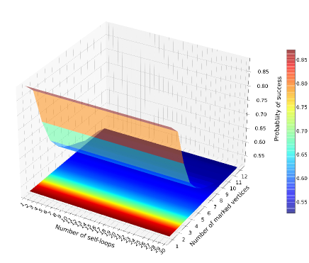
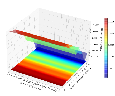
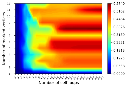
However, when we consider the multiple self-loops and the partial phase inversion, we can obtain equal or higher maximum probabilities of success depending on the weight $l$ used. The results of the MSLQW-PPI behavior are shown in Figures 2 and 4. They present the results obtained using the partial phase inversion of the target states as well as the maximum probability of success and coefficient of variation ($\sigma_{w}/\bar{w}$ – standard deviation normalized by the mean value) according to the number of self-loops and marked vertices. The level of dispersion shown in the results describes a behavior where the maximum success probabilities have a minor coefficient of variation. Figures 2a and 2b shows the probability of success for the weights $l=n/N$ and $l=(n/N)\cdot k$. The maximum probability $p=0.888$ and $p=0.999$ is reached when $k=2$ and $m=1$. The probability of success $p=0.888$ is also achieved with the weight $l=(n/N)\cdot k$, with $k=2$ marked vertices, and $m=2$ self-loops. These results are similar to those obtained by Souza et al. (2021).

(a)

(b)

(c)

(d)

Figure 2: The probability of success of theMSLQW-PPIto search for non-adjacent marked vertices with $n=12$ and $N=4096$ vertices. LABEL:sub@fig:probability-distribution-non-neighbors-n-N weight value $l=n/N$. LABEL:sub@fig:probability-distribution-non-neighbors-n-N weight value $l=(n/N)\cdot k$. LABEL:sub@fig:probability-distribution-non-neighbors-n-N-standard-deviation and LABEL:sub@fig:probability-distribution-non-neighbors-n-N-k-standard-deviation represent the coefficient of variation of the results presented in LABEL:sub@fig:probability-distribution-non-neighbors-n-N and LABEL:sub@fig:probability-distribution-non-neighbors-n-N-k, respectively. The results for coefficients of variation are represented in percentage terms.

Compared to quantum walks without self-loop, adding self-loops at each vertex of the structure that represents the time evolution of the walker improves the search capability of the quantum algorithms based on quantum walks and increases the probability of success. However, the self-loops have a strong dependence on the weight value. As we see in Fig. 2, the weight values proposed by Rhodes and Wong (2020) and Souza et al. (2021) are ideal for using a single self-loop. Therefore, for our approach, it is necessary to define the best weight value for using multiple self-loops. Most of the weights defined in previous works for structures such as a complete graph, hypercube, one-dimensional grid, and two-dimensional grid consider three main parameters: the vertex degree, the total number of vertices, and the number of marked vertices. Two weight values were already defined by Rhodes and Wong (2020) and Souza et al. (2021) as ideal for searching for one and multiple marked vertices in the hypercube, respectively: $l=n/N$ and $l=(n/k)\cdot k$, where $n$ is the degree of the vertices, $N$ the number of vertices, and $k$ the number of marked vertices.

The idea here is to propose two new weight values based on those previous ideal weight values used to search for one and multiple vertices in the hypercube. We introduce a new parameter in the weight composition: the exponent in the numerator. Considering that the weights $l=n/N$ and $l=(n/N)\cdot k$ has an exponent equal to $1$ in the numerator, we can consider other values for this parameter. We can modify the scale of weight values through this new parameter. In this article, we restrict the analysis to the integer exponent of value $2$ as the initial choice. So we have two new weights

$$l=\left(\frac{n^{2}}{N}\right),\text{ and }l=\left(\frac{n^{2}}{N}\right)\cdot k.$$

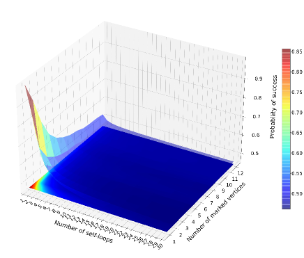
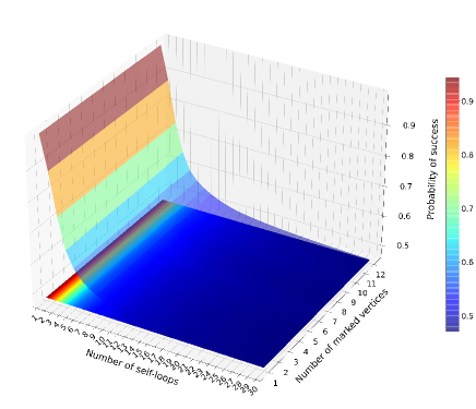
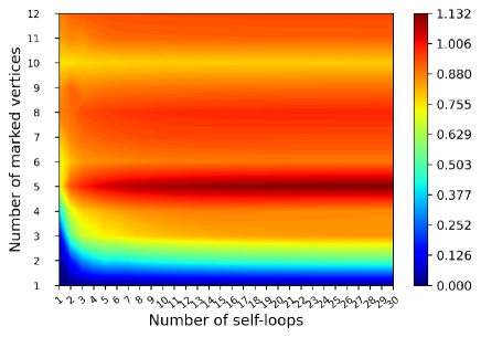
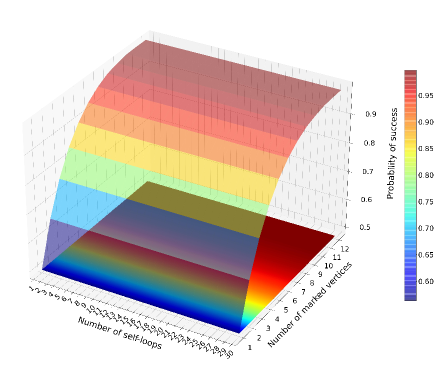
Fig. 3 shows the probability of success of the lackadaisical quantum walk using the two new weight values with multiple self-loops at each vertex in the hypercube to search multiple marked vertices. The phase of all target states components representing the $m$ self-loops is flipped. Figures 3a and 3b show the maximum probability of success for the weight values $l=n^{2}/N$ and $l=(n^{2}/N)\cdot k$, respectively. In these two cases, the probability of success is affected by the number of marked vertices, reaching a probability of approximately $p=0.99$ only when $k=12$ for the weight value $l=n^{2}/N$. Note that the behavior is the same as in Fig. 1, i.e., from the perspective that using one or more self-loops is equivalent. Although the weights are different, the behavior is the same independent of the number of self-loops.

(a)

(b)

(c)

(d)

Figure 3: The probability of success of the lackadaisical quantum walk in the hypercube with multiple self-loops to search for non-adjacent marked vertices with $n=12$ and $N=4096$ vertices. The phase of all state components that represent the self-loops is inverted. LABEL:sub@fig:probability-distribution-non-neighbors-all-signs-n-2-N weight value $l=n^{2}/N$. LABEL:sub@fig:probability-distribution-non-neighbors-all-signs-n-2-N-k weight value $l=(n^{2}/N)\cdot k$. LABEL:sub@fig:superficie-n-2-N-non-neighbors-standard-deviation-all-phase-invertion and LABEL:sub@fig:superficie-n-2-N-k-non-neighbors-standard-deviation-all-phase-invertion represent the coefficient of variation of the results presented in LABEL:sub@fig:probability-distribution-non-neighbors-n-N and LABEL:sub@fig:probability-distribution-non-neighbors-n-N-k, respectively. The results for coefficients of variation are represented in percentage terms.

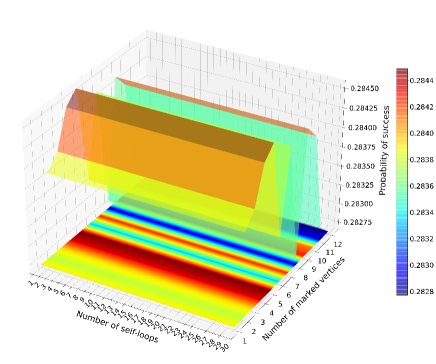
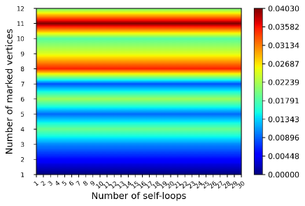
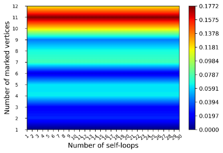
Analyzing the coefficient of variation of the results described in Fig. 3 we observe a different behavior than what occurs with the partial phase inversion, where the small coefficient of variation coincides with the maximum success probabilities. In Figures 3a and 3c for $k=\{2,3,7\}$ we have the smallest variations, however, the success probabilities are $p\approx\{0.489,0.640,0.929\}$. For $k=\{8,11\}$ the success probabilities are $p\approx\{0.958,0.996\}$, and we obtained the biggest variations. In the results shown in Figures 3b and 3d, the same behavior occurs, i.e, the smallest variations do not coincide with the maximum success probabilities. This indicates that the total phase inversion of the target state and the $k$ number of marked vertices make the procedure more unstable.

Fig. 4a shows the maximum probability of success for the partial inversion of the target states, and as already stated Fig. 3a shows the maximum probability of success where the phase of all target state components is inverted, both for the weight value $l=(n^{2}/N)$. In Fig. 4a we obtain success probabilities close to $1$ with up to $m=6$ self-loops. In Fig. 3a the coefficient of variation points to an unstable behavior, i.e., the most elevated probabilities of success do not coincide with the smallest coefficient of variations. However, in Fig. 4a the highest probabilities of success coincide with the smallest variations and therefore have a stable behavior. Table 2 shows that in most of the results applying partial phase inversion, there was an improvement in the maximum probability of success.

Table 2: Comparison between the probability of success and number of self-loops for two scenarios. The column for Fig. 3a represents the results where the phase of all self-loops is reversed. The column for Fig. 4a is for the case where the phase of only one self-loop is inverted. Both using the weight $l=n^{2}/N$. The acronym cv means the coefficient of variation.

	Figures
	3a			4a
k	p	m	cv	p	m	cv
2	0.48	1	5.234e-05	0.99	6	3.536e-04
3	0.64	1	1.050e-04	0.99	4	2.177e-04
4	0.75	1	1.922e-04	0.99	3	9.214e-05
5	0.83	1	9.214e-05	0.99	2	1.922e-04
6	0.88	1	2.177e-04	0.99	2	1.922e-04
7	0.92	1	8.130e-05	0.99	2	1.922e-04
8	0.95	1	3.536e-04	0.97	2	1.922e-04
9	0.97	1	2.477e-04	0.97	1	1.050e-04

Continuing the comparisons between the results obtained with the different weight values, again, we observed that it was possible to increase the probability of success with more than one self-loop and partial phase inversion. Fig. 2b shows the probability of success for the weight $l=(n/N)\cdot k$ with total phase inversion. Compared to the results presented in Fig. 4b that shows the probability of success for the weight $l=(n^{2}/N)\cdot k$ with partial phase inversion, the probabilities of success are similar and close to $1$, and what differs is the number of self-loops per vertex. In practical terms, using a single self-loop in this scenario is better. However, it is important to note that exists a relationship between the weight and the number of self-loops per vertex. Note that the number of self-loops may change depending on the weight value, in the case of Fig. 4b, the number of self-loops increased to 12.

Fig. 3b shows the maximum probability of success where the phase of all components of the target state is also inverted and Fig. 4b shows the maximum probability of success for the partial inversion of the target states, both for the weight value $l=(n^{2}/N)\cdot k$. This scenario showed a considerable gain in the maximum probability of success from $p=0.28$ (with $m=1$) to $p\approx 1$ (with $m=12$) self-loops to any number $k$ of the marked vertices.

(a)

(b)

(c)

(d)

Figure 4: The probability of success of the MSLQW-PPI to search for non-adjacent marked vertices with $n=12$ and $N=4096$ vertices. LABEL:sub@fig:probability-distribution-non-neighbors-n-2-N weight value $l=n^{2}/N$. LABEL:sub@fig:probability-distribution-non-neighbors-n-2-N-k weight value $l=(n^{2}/N)\cdot k$. LABEL:sub@fig:probability-distribution-non-neighbors-n-2-N-standard-deviation and LABEL:sub@fig:probability-distribution-non-neighbors-n-2-N-k-standard-deviation represent the coefficient of variation of the results presented in LABEL:sub@fig:probability-distribution-non-neighbors-n-2-N and LABEL:sub@fig:probability-distribution-non-neighbors-n-2-N-k, respectively. The results for coefficients of variation are represented in percentage terms.

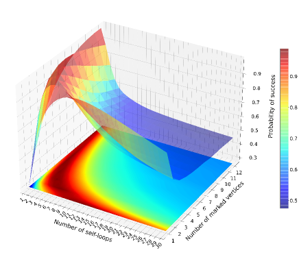
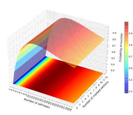
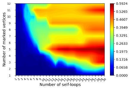
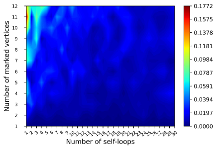
Finally, let us compare the results obtained from the partial inversion using all four weights. The results presented in Figures 2a and 2b show that the weights proposed by Rhodes and Wong (2020) and Souza et al. (2021), $l=n/N$ and $l=(n/N)\cdot k$ are not the ideal weights for MSLQW - PPI. However, with the use of the weights proposed in this work, $l=n^{2}/N$ and $l=(n^{2}/n)\cdot k$, we achieved the best results. We highlight the weight value $l=(n^{2}/n)\cdot k$. With this weight value, we obtained a stable behavior in most of the results. Table 3 shows the results of this comparison for the probability of success, number of self-loops, and coefficient of variation for all weights used in the MSLQW - PPI. Note that by modifying the weight scale and using various self-loops and partial phase inversion, it is possible to increase the probability of success.

Table 3: Comparison between probabilities of success for searching non-adjacent marked vertices and the number $m$ of self-loops. The results presented here refer to the search using partial phase inversion of the target state. From $k=4$ marked vertices, the success probabilities for weight $l=n/N$ remain below $p=0.65$, while for the other three weight values, the probability of success stays above $p=0.99$. The acronym cv means the coefficient of variation.

	Self-loop weights
	$l=n/N$			$l=(n/N)\cdot k$			$l=n^{2}/N$			$l=(n^{2}/N)\cdot k$
k	p	m	cv	p	m	cv	p	m	cv	p	m	cv
2	0.887	1	1.643e-04	0.999	1	8.259e-05	0.999	6	5.234e-05	0.999	12	2.810e-04
3	0.750	1	7.037e-04	0.999	1	1.144e-04	0.999	4	1.050e-04	0.999	12	2.095e-04
4	0.663	1	3.882e-03	0.999	1	1.221e-04	0.998	3	1.922e-04	0.999	12	6.324e-04

6 Conclusions

The lackadaisical quantum walk has a strong dependence on the self-loop weight value. We can see this fact in the results presented in all figures. For the cases where the phases of all self-loops are flipped, using a single self-loop per vertex is better. We can affirm the same for the results shown in Fig. 2.

When Wong (2015) proposed the lackadaisical quantum walk, he included $m$ integer self-loops at each vertex in the complete graph, which according to Rhodes and Wong (2020) is equivalent to having $m$ unweighted self-loops. However, Wong (2017) redefined the lackadaisical quantum walk, where each vertex with $m$ integer self-loops can be reduced to a quantum walk where each vertex has a single self-loop of real weight $l$. Note that the number of self-loops and the weight value $l$ are the main characteristics of this quantum walk. Our strategy differs in that we apply partial phase inversion and consider a real-valued weight $l$ and equally distribute it in $m$ self-loops in each vertex, i.e., m self-loops of non-integer weight value. In addition to using the two existing weight values in the literature to perform our experiments, we can contribute to the proposal of two new weight values. As the vertex degree is one of the parameters used in many works to define the weights assigned to self-loops, we suggest a modification that adds an exponent $\alpha$ to the numerator. Initially, we set the value of the exponent to an integer and equal to $\alpha=2$.

Quantum interference is essential in developing quantum algorithms (McMahon, 2007). The interference caused by the phase inversion operation, jointly with the average inversion operation, amplifies the target states’ amplitudes. It allows Grover’s search algorithm a certain probability of finding the desired state (Grover, 1996). The self-loops are redundant elements within the structure that composes the states of the quantum system. When we interfered jointly by flipping the phase of the $m$ self-loops, making them indistinguishable, we saw that it was equivalent to using a single self-loop. However, when we invert the phase of one of the $m$ self-loops, we empirically observe that the behavior caused by the constructive and destructive interference between the $m$ self-loops are analogous to those observed between the states that represent the vertices as a whole, i.e., most of the energy of the $m$ self-loops is retained in the phase-inverted self-loop. Preliminary results indicate that the phase inversion of a single self-loop $\circlearrowleft_{\tau}$ is sufficient to obtain the results presented in this work. Thus, the phase inversion and mean inversion operations individually act on the $m$ self-loops. In this way, the amplitude of the self-loop $\ket{\vec{x},\circlearrowleft_{0}}$ is amplified, for example. This behavior is interesting because it launches a new perspective on quantum interference in developing quantum algorithms.

To obtain the average behavior based on the relative position of the marked vertices, each simulation was performed on a sample that contains a number $k$ of distinctly marked vertices, that is, without replacement. Thus, verifying whether the relative position of non-adjacent marked vertices influences the results is possible. According to the results, the relative position of non-adjacent marked vertices does not significantly affect considering a numerical precision of four digits. Furthermore, the coefficient of variation indicates that the number $m$ of self-loops and the number $k$ of marked vertices influence the results. We used the coefficient of variation to analyze the results’ dispersion level. We observe that for MSLQW-PPI when we have the slightest standard deviations, the maximum probabilities of success scale to values close to $1$. The percentage variations around the mean are not significant. However, the behavior is stable for MSLQW-PPI, where there are slight variations. The results are more influenced by the number of marked vertices and the number of self-loops than by the relative position of the non-adjacent marked vertices. As we can see from the results, the multiple self-loops are an essential tool to improve the success probability of searching multiple marked vertices on the hypercube. Parameters such as weight value, weight distribution strategies, and phase inversion operation contributed to the results of this work.

In this work, the marked vertices are all non-adjacent. According to Souza et al. (2021), the type of marked vertices can interfere with the result of the quantum walk on the hypercube. Therefore, in future works, we intend to use the MSLQW-PPI to search for multiple adjacent marked vertices on the hypercube. We also intend to apply this methodology to evaluate the MSLQW-PPI in other $d$-regular structures. We intend to analyze other exponent values $\alpha$ for the composition of the weights $l=\{n^{\alpha}/N,(n^{\alpha}/N)\cdot k\}$, including real values, i.e., $\{\alpha\in\mathbb{R}\mid\alpha\neq 1\}$. It is possible to use an evolutionary search algorithm to define the best exponent $\alpha$ value capable of maximizing the probability of success and minimizing the number of self-loops influencing the current proposal. We intend to propose other strategies to distribute weight values, such as providing distinct self-loop weight values for marked vertices. Another possible path for deeper investigation is to analyze the phase inversion of multiple self-loops, i.e., $s\neq 1$, or to consider the partial inversion of edges $i$ that are not self-loops. Furthermore, proposing a variation of Grover’s search algorithm could also be a promising direction for future efforts.

References

- Shenvi et al. [2003] Neil Shenvi, Julia Kempe, and K Birgitta Whaley. Quantum random-walk search algorithm. Physical Review A, 67(5):052307, 2003.
- Grover [1996] Lov K Grover. A fast quantum mechanical algorithm for database search. In Proceedings of the twenty-eighth annual ACM symposium on Theory of computing, pages 212–219, 1996.
- Potoček et al. [2009] V Potoček, Aurél Gábris, Tamás Kiss, and Igor Jex. Optimized quantum random-walk search algorithms on the hypercube. Physical Review A, 79(1):012325, 2009.
- Hein and Tanner [2009] Birgit Hein and Gregor Tanner. Quantum search algorithms on the hypercube. Journal of Physics A: Mathematical and Theoretical, 42(8):085303, 2009.
- Hoyer and Meyer [2009] Stephan Hoyer and David A Meyer. Faster transport with a directed quantum walk. Physical Review A, 79(2):024307, 2009.
- Wong [2015] Thomas G Wong. Grover search with lackadaisical quantum walks. Journal of Physics A: Mathematical and Theoretical, 48(43):435304, 2015.
- Wong [2017] Thomas G Wong. Coined quantum walks on weighted graphs. Journal of Physics A: Mathematical and Theoretical, 50(47):475301, 2017.
- Rhodes and Wong [2020] Mason L Rhodes and Thomas G Wong. Search on vertex-transitive graphs by lackadaisical quantum walk. Quantum Information Processing, 19(9):1–16, 2020.
- Souza et al. [2021] Luciano S Souza, Jonathan H A Carvalho, and Tiago A E Ferreira. Lackadaisical quantum walk in the hypercube to search for multiple marked vertices. In Brazilian Conference on Intelligent Systems, pages 249–263. Springer, 2021.
- Wang et al. [2017] Huiquan Wang, Jie Zhou, Junjie Wu, and Xun Yi. Adjustable self-loop on discrete-time quantum walk and its application in spatial search. arXiv preprint arXiv:1707.00601, 2017.
- Rhodes and Wong [2019a] Mason L Rhodes and Thomas G Wong. Quantum walk search on the complete bipartite graph. Physical Review A, 99(3):032301, 2019a.
- Rapoza and Wong [2021] Jacob Rapoza and Thomas G Wong. Search by lackadaisical quantum walk with symmetry breaking. Physical Review A, 104(6):062211, 2021.
- McMahon [2007] David McMahon. Quantum computing explained. John Wiley & Sons, 2007.
- Wong [2018] Thomas G Wong. Faster search by lackadaisical quantum walk. Quantum Information Processing, 17(3):1–9, 2018.
- Rhodes and Wong [2019b] Mason L Rhodes and Thomas G Wong. Search by lackadaisical quantum walks with nonhomogeneous weights. Physical Review A, 100(4):042303, 2019b.
- Giri and Korepin [2020] Pulak Ranjan Giri and Vladimir Korepin. Lackadaisical quantum walk for spatial search. Modern Physics Letters A, 35(08):2050043, 2020.
- Carvalho et al. [2023] Jonathan H A Carvalho, Luciano S Souza, Fernando M Paula Neto, and Tiago A E Ferreira. On applying the lackadaisical quantum walk algorithm to search for multiple solutions on grids. Information Sciences, 622:873–888, 2023.
- Aharonov et al. [1993] Yakir Aharonov, Luiz Davidovich, and Nicim Zagury. Quantum random walks. Physical Review A, 48(2):1687, 1993.
- Ambainis et al. [2012] Andris Ambainis, Artūrs Bačkurs, Nikolajs Nahimovs, Raitis Ozols, and Alexander Rivosh. Search by quantum walks on two-dimensional grid without amplitude amplification. In Conference on Quantum Computation, Communication, and Cryptography, pages 87–97. Springer, 2012.
- Zhang et al. [2018] Jingyuan Zhang, Yonghong Xiang, and Weigang Sun. A discrete random walk on the hypercube. Physica A: Statistical Mechanics and its Applications, 494:1–7, 2018.
- Saha et al. [2022] Amit Saha, Ritajit Majumdar, Debasri Saha, Amlan Chakrabarti, and Susmita Sur-Kolay. Faster search of clustered marked states with lackadaisical quantum walks. Quantum Information Processing, 21(8):1–13, 2022.
- Tanaka et al. [2022] Hajime Tanaka, Mohamed Sabri, and Renato Portugal. Spatial search on johnson graphs by continuous-time quantum walk. Quantum Information Processing, 21(2):1–13, 2022.
- Qu et al. [2022] Dengke Qu, Samuel Marsh, Kunkun Wang, Lei Xiao, Jingbo Wang, and Peng Xue. Deterministic search on star graphs via quantum walks. Physical Review Letters, 128(5):050501, 2022.
- Venegas-Andraca [2012] Salvador Elías Venegas-Andraca. Quantum walks: a comprehensive review. Quantum Information Processing, 11(5):1015–1106, 2012.
- Kempe [2002] Julia Kempe. Quantum random walks hit exponentially faster. arXiv preprint quant-ph/0205083, 2002.
- Moore and Russell [2002] Cristopher Moore and Alexander Russell. Quantum walks on the hypercube. In International Workshop on Randomization and Approximation Techniques in Computer Science, pages 164–178. Springer, 2002.
- Høyer and Yu [2020] Peter Høyer and Zhan Yu. Analysis of lackadaisical quantum walks. arXiv preprint arXiv:2002.11234, 2020.
- Yu [2018] Zhan Yu. Searching faster using self-loops in quantum walks. University of Calgary, 2018.
- Santos et al. [2023] Henrique C T Santos, Luciano S Souza, Jonathan H A Carvalho, and Tiago A E Ferreira. Pesc–parallel experiment for sequential code. arXiv preprint arXiv:2301.05770, 2023.