Analytic distribution of the optimal cross-correlation statistic for stochastic gravitational-wave-background searches using pulsar timing arrays

Abstract

We show via both analytical calculation and numerical simulation that the optimal cross-correlation statistic (OS) for stochastic gravitational-wave-background (GWB) searches using data from pulsar timing arrays follows a generalized chi-squared (GX2) distribution—i.e., a linear combination of chi-squared distributions with coefficients given by the eigenvalues of the quadratic form defining the statistic. This observation is particularly important for calculating the frequentist statistical significance of a possible GWB detection, which depends on the exact form of the distribution of the OS signal-to-noise ratio (S/N) $\hat{\rho}\equiv\hat{A}_{\rm gw}^{2}/\sigma_{0}$ in the absence of GW-induced cross correlations (i.e., the null distribution). Previous discussions of the OS have incorrectly assumed that the analytic null distribution of $\hat{\rho}$ is well-approximated by a zero-mean unit-variance Gaussian distribution. Empiricial calculations show that the null distribution of $\hat{\rho}$ has “tails” which differ significantly from those for a Gaussian distribution, but which follow (exactly) a GX2 distribution. So, a correct analytical assessment of the statistical significance of a potential detection requires the use of a GX2 distribution.

I Introduction

Nanohertz-frequency gravitational waves (GWs) from supermassive binary black holes (SMBBHs) should be detected in the near future by pulsar timing arrays [1, 2, 3]. The North American Nanohertz Observatory for Gravitational Waves (NANOGrav) [4] has already reported strong statistical evidence for a common-spectrum red-noise process across pulsars in a search for an isotropic stochastic gravitational-wave background (GWB) in their 12.5-year dataset [5]. This finding was followed by analyses of Parkes Pulsar Timing Array (PPTA) data [6], European Pulsar Timing Array (EPTA) data [7], as well as the International Pulsar Timing Array (IPTA) second data release [8]. All of these studies confirmed the presence of a common-spectrum red-noise process across pulsars. Currently, however, there is little evidence for the quadrupolar spatial correlations [9] necessary to make a confident claim of detection of the GWB. Analytical work and simulations [1, 2, 3] show that the additional statistical evidence in the spatial correlations needed to claim a detection will come after analyzing larger datasets with more pulsars and longer data spans, or combining existing datasets from other pulsar timing array collaborations through the IPTA.

A computationally efficient technique used by the pulsar timing community to calculate the significance of the cross-correlations is the so-called optimal statistic (OS) [10, 11, 12]. This statistic is an unbiased estimator for the square of the GWB amplitude $A_{\rm gw}^{2}$ derived by maximizing the logarithm of the likelihood ratio, and it can be related to the Bayesian odds ratio between a model with correlations and a model without correlations via the Laplace approximation [13]. The work in this paper concerns the calculation of the probability distribution for the OS signal-to-noise ratio (S/N) $\hat{\rho}\equiv\hat{A}_{\rm gw}^{2}/\sigma_{0}$, where $\sigma_{0}^{2}$ is the variance of the estimator $\hat{A}_{\rm gw}^{2}$ in the absence of GW-induced spatial correlations.

The distribution for $\hat{\rho}$ in the absence of such spatial correlations is called the null distribution, and is denoted by $p(\hat{\rho}|H_{0})$. $H_{0}$ is the null hypothesis—i.e., the hypothesis that there are no GW-induced spatial correlations in the data. Although $H_{0}$ assumes no spatial correlations, it does allow for the presence of a non-zero common-spectrum red-noise process as is currently observed, whose amplitude $A_{\rm cp}$ is determined from a joint noise analysis for the pulsars in the array. As such, the null distribution $H_{0}$ depends on the particular value of $A_{\rm cp}$—i.e., $H_{0}=H_{0}(A_{\rm cp})$. However, to simplify the notation in what follows, we will not explicitly display the $A_{\rm cp}$ dependence of $H_{0}$, although we will investigate the dependence of the null distribution on the amplitude and spectral shape of the common-spectrum red-noise process.

Given the null distribution, we can calculate the probability that our measured S/N, denoted $\hat{\rho}_{\rm obs}$, could have resulted from noise alone. This is called the $p$-value and is defined as

$$p\equiv{\rm Prob}(\hat{\rho}>\hat{\rho}_{\rm obs}|H_{0})\equiv\int_{\hat{\rho}_{\rm obs}}^{\infty}\>p(\hat{\rho}|H_{0})\,{\rm d}\hat{\rho}\,.$$ (1)

The false alarm probability $\alpha$ is similarly defined:

$$\alpha\equiv{\rm Prob}(\hat{\rho}>\hat{\rho}_{\rm th}|H_{0})\equiv\int_{\hat{\rho}_{\rm th}}^{\infty}\>p(\hat{\rho}|H_{0})\,{\rm d}\hat{\rho}\,,$$ (2)

where $\hat{\rho}_{\rm th}$ is the detection threshold, above which one would reject the null hypothesis and claim detection of a GWB. The detection threshold is typically chosen so that the false alarm probability has a sufficiently small value, e.g. $\alpha<1\times 10^{-3}$ above that threshold. Note that the right hand sides of both (1) and (2) can also be written as $1-{\rm CDF}(x|H_{0})$, where ${\rm CDF}(x)$ is the standard cumulative distribution function and $x=\hat{\rho}_{\rm obs}$ and $\hat{\rho}_{\rm th}$, respectively.

By construction, both the $p$-value and the false alarm probability (or, equivalently, the choice of the detection threshold) depend on the detailed form of the null distribution. In previous work [10, 11, 12], appealing to the central limit theorem (and also for simplicity), this distribution was assumed to be Gaussian. Here, we show that the null distribution for the OS follows a generalized chi-squared (GX2) distribution [14] and we explore the consequences of this observation. (A paper by Cordes and Shannon [15] also noted that the distribution of the cross-correlation statistic was highly non-Gaussian and skewed, but did not identify it as a GX2 distribution.) We show that differences between the GX2 and Gaussian distributions can be significant for current pulsar timing array configurations (defined by numbers of pulsars, observation spans, noise parameters, etc.), as well as the amplitude and spectral shape of the common-spectrum process, especially in the tails of the distribution. Thus, the GX2 distribution should be used to calculate more accurate $p$-values in the case of a GW detection. In particular, we show that the Gaussian distribution assumption for the null distribution of the OS leads to overestimates of the significance of a potential detection, i.e., smaller $p$-values, than for the GX2 distribution.

We also compare the GX2 and Gaussian distributions of the OS to the null distributions obtained from doing phase-shifts [16] and sky scrambles [17] of the PTA data. The phase-shifts are analogous to applying time-shifts in ground-based GW detectors, while sky scrambles replace the actual pulsar locations with random sky locations, thus breaking all spatial correlations except for the direction-independent monopole. Both of these techniques work well at removing GW-induced correlations, and are now standard methods to determine null distributions for our statistics, be it the OS or the Bayes factor, directly from our data [5]. We show that the GX2 distribution is an excellent fit to the phase-shifted / sky-scrambled data compared with the standard Gaussian approximation, especially in the tails of the distribution (where it matters most) at larger values of the OS signal-to-noise ratio $\hat{\rho}$.

The rest of the paper is organized as follows: In Sec. II, we summarize the results of [14], explaining how GX2 distributions arise whenever one has a (symmetric) quadratic combination of random variables satisfying a multivariate Gaussian distribution. We then show, in Sec. III, that the OS used for PTA searches is an example of such a quadratic combination, explicitly describing the various pieces that enter the calculation of the eigenvalues needed for the GX2 distribution. In Section IV, we first calculate GX2 distributions for the OS for several different sets of simulated data, in the absence of simulated GW-induced cross correlations. We show how these distributions depend on the relative contribution of red and white noise, the number of pulsars, fitting to a timing a model, etc., and compare these distributions with unit (i.e., standard normal) Gaussians, which often deviate significantly from the GX2 distributions in the tails of the distributions. We then compare the GX2 distribution for the OS with the null distribution of $\hat{\rho}$ obtained by phase-shifting the NANOGrav 12.5-yr data [5]. Finally, we conclude in Sec V by discussing possible extensions / modifications to the calculations presented here—e.g., which might simplify the calculation of GX2 distributions for realistic PTA datasets. Appendix A describes a simple “tail-fitting” approach that allows us to extrapolate the tail of the OS null distribution beyond empirically determined phase-shift or sky-scramble values.

II Mathematical formalism

By definition, the generalized chi-square (GX2) distribution is the probability distribution of a quadratic form of multivariate-Gaussian random variables $\mathbf{x}\sim{\cal N}(\boldsymbol{\mu},\boldsymbol{\Sigma})$:

$$q(\mathbf{x})\equiv\frac{1}{2}\mathbf{x}^{T}\mathbf{Q}_{2}\mathbf{x}+\mathbf{q}_{1}^{T}\mathbf{x}+q_{0}\,,$$ (3)

where

$$p(\mathbf{x}|\boldsymbol{\mu},\boldsymbol{\Sigma})=\frac{1}{\sqrt{{\rm det}(2\pi\boldsymbol{\Sigma}})}e^{-\frac{1}{2}(\mathbf{x}-\boldsymbol{\mu})^{T}\boldsymbol{\Sigma}^{-1}(\mathbf{x}-\boldsymbol{\mu})}\,.$$ (4)

Here $q_{0}$ is a real constant, $\mathbf{q}_{1}$ is a real vector of the same dimension as $\mathbf{x}$, and $\mathbf{Q}_{2}$ is a real symmetric matrix $\mathbf{Q}_{2}^{T}=\mathbf{Q}_{2}$. As we shall describe in Sec. III, the cross-correlation statistic that we are interested in has the simpler form

$$q(\mathbf{x})\equiv\frac{1}{2}\mathbf{x}^{T}\mathbf{Q}\mathbf{x}\,,\qquad\mathbf{x}\sim{\cal N}(\mathbf{0},\boldsymbol{\Sigma})\,.$$ (5)

In this last equation we have dropped the subscript 2 from $\mathbf{Q}_{2}$ to simplify the notation, since there is no potential to confuse it with a linear or constant term. We will work with this simpler form for the rest of the paper.

To use the formalism of [14] to explicitly compute the GX2 distribution of $q(\mathbf{x})$, we need to write (5) as a linear superposition of standard normal distributions $\mathbf{v}\sim{\cal N}(\mathbf{0},\mathbf{1})$. This is done via a series of eigenvalue/eigenvector decompositions which we summarize below:

Following [14], we start by converting $\mathbf{x}\sim{\cal N}(\mathbf{0},\boldsymbol{\Sigma})$ to a vector of uncorrelated standard normal distributions $\mathbf{z}\sim{\cal N}(\mathbf{0},\mathbf{1})$ by finding the eigenvalues and eigenvectors of $\boldsymbol{\Sigma}$:

$$\mathbf{D}=\mathbf{E}^{T}\boldsymbol{\Sigma}\mathbf{E}\quad{\rm or}\quad\boldsymbol{\Sigma}=\mathbf{E}\mathbf{D}\mathbf{E}^{T}\,,$$ (6)

where $\mathbf{D}$ is a diagonal matrix of eigenvalues $\mathbf{D}={\rm diag}(\sigma^{2}_{1},\sigma^{2}_{2},\cdots)$ and $\mathbf{E}$ is an orthogonal matrix (i.e., $\mathbf{E}^{T}=\mathbf{E}^{-1}$) whose columns are the corresponding (orthonormal) eigenvectors of $\boldsymbol{\Sigma}$. Since $\boldsymbol{\Sigma}$ is a covariance matrix, we are guaranteed that its eigenvalues are all positive, hence the form $\sigma^{2}_{1}$, $\sigma^{2}_{2}$, $\ldots$. We then take the square root of $\mathbf{D}$:

$$\boldsymbol{\Lambda}\equiv\sqrt{\mathbf{D}}\,,$$ (7)

for which

$$\mathbf{x}^{T}\boldsymbol{\Sigma}^{-1}\mathbf{x}=\mathbf{x}^{T}\mathbf{E}\mathbf{D}^{-1}\mathbf{E}^{T}\mathbf{x}=\mathbf{x}^{T}\mathbf{E}\boldsymbol{\Lambda}^{-1}\boldsymbol{\Lambda}^{-1}\mathbf{E}^{T}\mathbf{x}=\mathbf{z}^{T}\mathbf{1}\mathbf{z}\,,$$ (8)

where

$$\mathbf{z}\equiv\boldsymbol{\Lambda}^{-1}\mathbf{E}^{T}\mathbf{x}\quad\Leftrightarrow\quad\mathbf{x}=\mathbf{E}\boldsymbol{\Lambda}\mathbf{z}\,.$$ (9)

In terms of $\mathbf{z}$ the quadratic combination (5) has the form

$$q(\mathbf{x})=\frac{1}{2}\mathbf{z}^{T}\tilde{\mathbf{Q}}\mathbf{z}\,,\qquad\mathbf{z}\sim{\cal N}(\mathbf{0},\mathbf{1})\,,$$ (10)

where

$$\tilde{\mathbf{Q}}\equiv\boldsymbol{\Lambda}^{T}\mathbf{E}^{T}\mathbf{Q}\mathbf{E}\boldsymbol{\Lambda}\,.$$ (11)

The final step is to diagonalize $\tilde{\mathbf{Q}}$, by finding its eigenvalues $(\tilde{e}_{1},\tilde{e}_{2},\cdots)$ and the orthogonal matrix of eigenvectors $\mathbf{U}$. This gives

$$\tilde{\mathbf{Q}}=\mathbf{U}{\rm diag}(\tilde{e}_{1},\tilde{e}_{2},...)\mathbf{U}^{T}\,,$$ (12)

for which

$$q(\mathbf{x})=\frac{1}{2}\sum_{i}\tilde{e}_{i}v_{i}^{2}\,,\quad{\rm where}\quad\mathbf{v}\equiv\mathbf{U}^{T}\mathbf{z}\sim{\cal N}(\mathbf{0},\mathbf{1})\,.$$ (13)

(Note that $\mathbf{v}$ is standard normal since $\mathbf{U}$ is an orthogonal matrix and $\mathbf{z}$ is standard normal.) Since the probability distribution of the square of a standard normal distribution is chi-squared distributed with 1 degree of freedom (DOF), it follows that $q(\mathbf{x})$ is a general linear combination of $\chi^{2}_{1}$ distributions, which is the form of the generalized chi-squared distribution discussed in Ref. [14]. The analytic form of this distribution for the quadratic form (5) is completely specified by the eigenvalues of $\tilde{\mathbf{Q}}$ defined by (11), (6), and (7).

Note that the mean and variance of $q(\mathbf{x})$ can be simply written in terms of sums (and sums of squares) of the eigenvalues: used to construct the optimal statistic.

$$\mu_{q}\equiv\langle q\rangle=\frac{1}{2}\sum_{i}\tilde{e}_{i}\qquad{\rm and}\qquad\sigma^{2}_{q}\equiv\langle q^{2}\rangle-\langle q\rangle^{2}=\frac{1}{2}\sum_{i}\tilde{e}_{i}^{2}\,,$$ (14)

where $\langle\ \rangle$ denotes expectation value. The above results follow from the expansion (13) with the $v_{i}^{2}\sim\chi^{2}_{1}$ being statistically independent of one another, and each having ${\rm mean}=1$ and ${\rm variance}=2$.

III Application to the optimal statistic for PTA searches for GWBs

Now we show that different forms of the OS used for PTA searches for GWBs are examples of GX2 distributions. For more details regarding the OS, we refer the reader to see [10, 11, 12].

III.1 Optimal statistic S/N and GWB amplitude estimator

The optimal statistic S/N for PTA searches for GWBs is typically written as

$$\hat{\rho}\equiv{\hat{A}^{2}_{\rm gw}}/{\sigma_{0}}\,,$$ (15)

where

$$\hat{A}^{2}_{\rm gw}\equiv{\cal N}\sum_{a<b}\mathbf{r}^{T}_{a}\mathbf{P}_{a}^{-1}\tilde{\mathbf{S}}_{ab}\mathbf{P}_{b}^{-1}\mathbf{r}_{b}\,,$$ (16)

$$\sigma_{0}\equiv{\cal N}^{1/2}\,,$$ (17)

$${\cal N}\equiv\left(\sum_{a<b}{\rm tr}\left[\mathbf{P}_{a}^{-1}\tilde{\mathbf{S}}_{ab}\mathbf{P}_{b}^{-1}\tilde{\mathbf{S}}_{ba}\right]\right)^{-1}\,.$$ (18)

In the above expressions, $\hat{A}_{\rm gw}^{2}$ is an estimator of the (squared) amplitude of the GW signal, $\sigma_{0}^{2}$ is its variance in the absence of GW-induced spatial correlations, and $\cal N$ is a normalization factor constructed from terms involving the total auto-correlated power and cross-correlated power in pulsars labeled by $a$, $b$ (more about these expressions below). More compactly,

$$\hat{\rho}\equiv\sum_{a<b}\mathbf{r}_{a}^{T}\mathbf{Q}_{ab}\mathbf{r}_{b}=\frac{1}{2}\sum_{a,b}\mathbf{r}_{a}^{T}\mathbf{Q}_{ab}\mathbf{r}_{b}\,,$$ (19)

where

$$\mathbf{Q}_{aa}\equiv\mathbf{0}\,,\qquad\mathbf{Q}_{ab}\equiv{\cal N}^{1/2}\mathbf{P}_{a}^{-1}\tilde{\mathbf{S}}_{ab}\mathbf{P}_{b}^{-1}$$ (20)

define the (symmetric) quadratic form for $\hat{\rho}$. Note that summations denoted by $\sum_{a<b}$ run over distinct pulsar pairs, while $\sum_{a,b}\equiv\sum_{a}\sum_{b}$ double counts the pulsar pairs (hence the factor of 1/2 in (19)) and also includes the auto-correlations (which don’t contribute to $\hat{\rho}$ since $\mathbf{Q}_{aa}=\mathbf{0}$).

The data $\mathbf{r}$ are zero-mean multivariate Gaussian random variables defined by

$$p(\mathbf{r}|\vec{\theta})=\frac{1}{\sqrt{{\rm det}(2\pi\boldsymbol{\Sigma})}}\exp\left(-\frac{1}{2}\mathbf{r}^{T}\boldsymbol{\Sigma}^{-1}\mathbf{r}\right)\,,$$ (21)

where

$$\boldsymbol{\Sigma}\equiv\langle\mathbf{r}\mathbf{r}^{T}\rangle=\begin{pmatrix}\mathbf{P}_{1}&\mathbf{S}_{12}&\cdots&\mathbf{S}_{1M}\\ \mathbf{S}_{21}&\mathbf{P}_{2}&\cdots&\mathbf{S}_{2M}\\ \vdots&\vdots&\ddots&\vdots\\ \mathbf{S}_{M1}&\mathbf{S}_{M2}&\cdots&\mathbf{P}_{M}\\ \end{pmatrix}$$ (22)

and

$$\mathbf{P}_{a}\equiv\mathbf{G}_{a}^{T}\mathbf{N}_{a}\mathbf{G}_{a}\,,\qquad\mathbf{S}_{ab}\equiv\mathbf{G}_{a}^{T}\mathbf{X}_{ab}\mathbf{G}_{b}\,,\qquad a,b=1,2,\cdots,M\,.$$ (23)

Here, $M$ denotes the number of pulsars, and $\mathbf{G}_{a}$ is the $G$-matrix for pulsar $a$ [18], which encodes information about the timing-model fit

$$\mathbf{r}_{a}=\mathbf{G}^{T}_{a}\,\boldsymbol{\delta}\mathbf{t}_{a}\,,\qquad a=1,2,\cdots,M\,,$$ (24)

where $\boldsymbol{\delta}\mathbf{t}_{a}$ are the timing residuals for pulsar $a$. If we denote the number of TOAs for pulsar $a$ by $N_{{\rm TOA},a}$ and the number of timing model parameters by $N_{{\rm par},a}$, then $\mathbf{G}_{a}$ has dimensions $N_{{\rm TOA},a}\times(N_{{\rm TOA},a}-N_{{\rm par},a})$, and $\mathbf{r}_{a}$ is a vector with components

$$[\mathbf{r}_{a}]_{\alpha_{a}}\,,\qquad\alpha_{a}=1,2,\cdots,N_{a}\equiv(N_{{\rm TOA},a}-N_{{\rm par},a})\,.$$ (25)

The covariance matrix $\boldsymbol{\Sigma}$ is thus a symmetric block matrix and has overall dimension $(N_{1}+N_{2}+\cdots+N_{M})\times(N_{1}+N_{2}+\cdots+N_{M})$.

The diagonal terms of the covariance matrix involve the autocorrelations

$$\mathbf{N}_{a}\equiv\langle\boldsymbol{\delta}\mathbf{t}_{a}\boldsymbol{\delta}\mathbf{t}^{T}_{a}\rangle=\int_{0}^{f_{\rm Nyq}}{\rm d}f\>\cos[2\pi f\boldsymbol{\tau}_{aa}]\,{\cal P}_{a}(f)+{\cal F}_{a}\mathbf{W}_{a}+{\cal Q}^{2}_{a}\mathbf{1}\,,$$ (26)

where the last two terms specify the white noise contributions, and

$${\cal P}_{a}(f)\equiv{\cal P}_{a}^{\rm red}(f)+{\cal P}_{\rm gw}(f)$$ (27)

consists of both intrinsic pulsar red noise and a potential common-spectrum red-noise process contribution most likely from the GWB. We assume that both of these red noise contributions can be described by power-law spectra

$${\cal P}_{a}^{\rm red}(f)\equiv\frac{A^{2}_{a}}{12\pi^{2}f^{3}}\left(\frac{f}{f_{\rm ref}}\right)^{2\alpha_{a}}\,,\qquad{\cal P}_{\rm gw}(f)\equiv\frac{A^{2}_{\rm gw}}{12\pi^{2}f^{3}}\left(\frac{f}{f_{\rm ref}}\right)^{2\alpha_{\rm gw}}\,.$$ (28)

For the GWB formed from the superposition of signals from inspiraling super-massive binary black holes in the centers of merging galaxies, $\alpha_{\rm gw}=-2/3$. Finally, $\boldsymbol{\tau}_{aa}$ is the time-lag matrix, whose components are given by $[\boldsymbol{\tau}_{aa}]_{ij}\equiv t_{i_{a}}-t_{j_{a}}$, which are the differences of the TOAs of the pulses from pulsar $a$.

The off-diagonal terms in the covariance matrix are assumed to have only a GWB contribution

$$\mathbf{X}_{ab}\equiv\langle\boldsymbol{\delta}\mathbf{t}_{a}\boldsymbol{\delta}\mathbf{t}^{T}_{b}\rangle=\Gamma_{ab}\int_{0}^{f_{\rm Nyq}}{\rm d}f\>\cos[2\pi f\boldsymbol{\tau}_{ab}]\,{\cal P}_{\rm gw}(f)\,,$$ (29)

where

$$\Gamma_{ab}\equiv\frac{1}{2}+\frac{3}{2}\left(\frac{1-\cos\xi_{ab}}{2}\right)\left[\ln\left(\frac{1-\cos\xi_{ab}}{2}\right)-\frac{1}{6}\right]+\frac{1}{2}\delta_{ab}$$ (30)

are the values of the Hellings-and-Downs function, $\Gamma_{ab}\equiv\Gamma(\xi_{ab})$, evaluated for two pulsars $a$ and $b$ separated by the angle $\xi_{ab}$, see [9]. The quantity

$$\tilde{\mathbf{S}}_{ab}\equiv\mathbf{G}^{T}_{a}\tilde{\mathbf{X}}_{ab}\mathbf{G}_{b}\,,$$ (31)

which enters the expression for the quadratic form $\mathbf{Q}_{ab}$, is a normalized version of $\mathbf{S}_{ab}$ defined in terms of

$$\tilde{\mathbf{X}}_{ab}\equiv\mathbf{X}_{ab}/A_{\rm gw}^{2}\,.$$ (32)

Note that these cross-correlations are proportional to the spectral shape of the GWB—i.e., they do not depend on its amplitude.

Finally, it is a simple matter to show that the GWB amplitude estimator $\hat{A}^{2}_{\rm gw}$ can also be written as a (symmetric) quadratic combination of the multivariate Gaussian random variables $\mathbf{r}$ with quadratic form

$$\mathbf{K}_{ab}\equiv{\cal N}^{1/2}\mathbf{Q}_{ab}\,.$$ (33)

So, according to the discussion in Sec. II, both $\hat{\rho}$ and $\hat{A}^{2}_{\rm gw}$ will be described by GX2 distributions. For calculating the distributions of these statistics in the absence of GW-induced spatial correlations (i.e., null distributions), we should set $\mathbf{X}_{ab}=\mathbf{0}$ in the definition of $\boldsymbol{\Sigma}$ and replace the GW contribution ${\cal P}_{\rm gw}(f)$ to $\mathbf{N}_{a}$ by a potential common-spectrum red-noise process ${\cal P}_{\rm cp}(f)$ (with amplitude $A_{\rm cp}$ and spectral index $\alpha_{\rm cp}$), which is common to all pulsars. (The normalized cross-correlation terms $\tilde{\mathbf{S}}_{ab}$ in $\mathbf{Q}_{ab}$ do not change since they involve the normalized cross-correlations $\tilde{\mathbf{X}}_{ab}$.) These null distributions are obviously also described by GX2 distributions since they are special cases of the non-null quadratic combinations.

Using (14), it follows the eigenvalues $\tilde{e}_{i}$ that specify the GX2 distribution for $\hat{\rho}\equiv A^{2}_{\rm gw}/\sigma_{0}$ in the absence of GW-induced spatial correlations satisfy:

$$\sum_{i}\tilde{e}_{i}=0\qquad{\rm and}\qquad\sum_{i}\tilde{e}_{i}^{2}=2\,.$$ (34)

These are consequences of $\hat{\rho}$ having zero mean and unit variance for the null distribution case.

III.2 Optimal statistic pulsar-pair cross-correlation estimators

One can also construct cross-correlation estimators for individual pulsar pairs:

$$\hat{\rho}_{ab}\equiv{\cal N}_{ab}\,\mathbf{r}^{T}_{a}\mathbf{P}_{a}^{-1}\bar{\mathbf{S}}_{ab}\mathbf{P}_{b}^{-1}\mathbf{r}_{b}\equiv\mathbf{r}^{T}_{a}\bar{\mathbf{Q}}_{ab}\mathbf{r}_{b}\,,\qquad a<b=1,2,\cdots,M\,,$$ (35)

where

$$\bar{\mathbf{Q}}_{ab}\equiv{\cal N}_{ab}\,\mathbf{P}_{a}^{-1}\bar{\mathbf{S}}_{ab}\mathbf{P}_{b}^{-1}\,,$$ (36)

$${\cal N}_{ab}\equiv\left({\rm tr}\left[\mathbf{P}_{a}^{-1}\bar{\mathbf{S}}_{ab}\mathbf{P}_{b}^{-1}\bar{\mathbf{S}}_{ba}\right]\right)^{-1}\,,$$ (37)

$$\bar{\mathbf{S}}_{ab}\equiv\mathbf{G}^{T}_{a}\bar{\mathbf{X}}_{ab}\mathbf{G}_{b}\,,$$ (38)

$$\bar{\mathbf{X}}_{ab}\equiv\mathbf{X}_{ab}/(\Gamma_{ab}A_{\rm gw}^{2})=\int_{0}^{f_{\rm Nyq}}{\rm d}f\>\cos[2\pi f\boldsymbol{\tau}_{ab}]\,\bar{{\cal P}}_{\rm gw}(f)\,,$$ (39)

$$\bar{{\cal P}}_{\rm gw}(f)\equiv\frac{1}{12\pi^{2}f^{3}}\left(\frac{f}{f_{\rm ref}}\right)^{2\alpha_{\rm gw}}\,.$$ (40)

Using

$$\langle\mathbf{r}_{a}\mathbf{r}_{b}^{T}\rangle=\mathbf{S}_{ab}\,,$$ (41)

it follows that $\hat{\rho}_{ab}$ is an unbiased estimator of the cross-correlated power in the GWB—i.e.,

$$\langle\hat{\rho}_{ab}\rangle=\Gamma_{ab}A_{\rm gw}^{2}\,,$$ (42)

with variance

$$\sigma^{2}_{ab}={\cal N}_{ab}+(A_{\rm gw}^{2})^{2}{\cal N}_{ab}^{2}\,{\rm tr}\,[\mathbf{P}_{a}^{-1}\bar{\mathbf{S}}_{ab}\mathbf{P}_{b}^{-1}\tilde{\mathbf{S}}_{ba}\mathbf{P}_{a}^{-1}\bar{\mathbf{S}}_{ab}\mathbf{P}_{b}^{-1}\tilde{\mathbf{S}}_{ba}]\,.$$ (43)

In the absence of GW-induced spatial correlations, the variance simplifies to

$$\sigma^{2}_{ab}={\cal N}_{ab}\equiv\sigma^{2}_{0,ab}\,.$$ (44)

Recall that $\Gamma_{ab}$ are the values of the Hellings-and-Downs function evaluated for different angular separations between the two pulsars labeled by $a$ and $b$. The matrix $\bar{\mathbf{X}}_{ab}$ is the time-domain representation of the spectral shape of the GW power spectrum, which (by its definition) is independent of the GWB amplitude $A_{\rm gw}$ and the spatial correlation coefficients $\Gamma_{ab}$. It depends on the pulsar pair $ab$ only via the discrete times $t_{i_{a}}$, $t_{j_{b}}$ of the timing residuals $\boldsymbol{\delta}\mathbf{t}_{a}$, $\boldsymbol{\delta}\mathbf{t}_{b}$, which enter the time-lag matrix $\boldsymbol{\tau}_{ab}$. This means that $\bar{\mathbf{X}}_{ab}$ is a rectangular matrix with dimensions $N_{{\rm TOA},a}\times N_{{\rm TOA},b}$.

Since $\hat{\rho}_{ab}=\hat{\rho}_{ba}$, we can write

$$\hat{\rho}_{ab}=\frac{1}{2}(\hat{\rho}_{ab}+\hat{\rho}_{ba})=\frac{1}{2}\left(\mathbf{r}^{T}_{a}\bar{\mathbf{Q}}_{ab}\mathbf{r}_{b}+\mathbf{r}^{T}_{b}\bar{\mathbf{Q}}_{ba}\mathbf{r}_{a}\right)=\frac{1}{2}\mathbf{x}^{T}\mathbf{Q}\mathbf{x}\,,$$ (45)

where

$$\mathbf{x}^{T}\equiv\begin{bmatrix}\mathbf{r}^{T}_{a}&\mathbf{r}^{T}_{b}\end{bmatrix}\,,\qquad\mathbf{Q}\equiv\begin{bmatrix}\mathbf{0}&\bar{\mathbf{Q}}_{ab}\\ \bar{\mathbf{Q}}_{ba}&\mathbf{0}\end{bmatrix}\,,\qquad\mathbf{x}\equiv\begin{bmatrix}\mathbf{r}_{a}\\ \mathbf{r}_{b}\end{bmatrix}\,.$$ (46)

Note that $\mathbf{Q}$ is a symmetric matrix since $\bar{\mathbf{Q}}_{ab}^{T}=\bar{\mathbf{Q}}_{ba}$. Note also that $\mathbf{x}\sim{\cal N}(\mathbf{0},\boldsymbol{\Sigma)}$, where

$$\boldsymbol{\Sigma}\equiv\langle\mathbf{x}\mathbf{x}^{T}\rangle=\begin{bmatrix}\mathbf{P}_{a}&\mathbf{S}_{ab}\\ \mathbf{S}_{ba}&\mathbf{P}_{b}\end{bmatrix}\,.$$ (47)

So given that $\hat{\rho}_{ab}$ is a symmetric quadratic combination of multivariate Gaussian random variables, it obeys a GX2 distribution.

If desired, one can express both the OS signal-to-noise ratio $\hat{\rho}$ and the GWB amplitude estimator $\hat{A}_{\rm gw}^{2}$ in terms of the pulsar-pair cross-correlation estimators $\hat{\rho}_{ab}$:

$$\hat{\rho}=\frac{\sum_{a<b}\Gamma_{ab}\hat{\rho}_{ab}/\sigma^{2}_{0,ab}}{\sqrt{\sum_{c<d}\Gamma_{cd}^{2}/\sigma^{2}_{0,cd}}}\qquad{\rm and}\qquad\hat{A}^{2}_{\rm gw}=\frac{\sum_{a<b}\Gamma_{ab}\hat{\rho}_{ab}/\sigma^{2}_{0,ab}}{\sum_{c<d}\Gamma_{cd}^{2}/\sigma^{2}_{0,cd}}\,.$$ (48)

These results are a consequence of $\tilde{\mathbf{S}}_{ab}=\Gamma_{ab}\bar{\mathbf{S}}_{ab}$ and the definitions (15), (16), and (35) of $\hat{\rho}$, $\hat{A}^{2}_{\rm gw}$, and $\hat{\rho}_{ab}$. Thus, $\hat{\rho}$ and $\hat{A}_{\rm gw}^{2}$ are simple noise-weighted and $\Gamma_{ab}$-matched linear combinations of the $\hat{\rho}_{ab}$.

IV Demonstration of the GX2 distribution on PTA data

The exact form of the GX2 distribution varies with the amplitude of the GW signal and the noise properties of the data. The characteristics of PTA noise have been studied extensively in the literature [19, 20, 21]. The considerations for PTA detector characterization vary widely from radiometer noise at the telescope receiver, to possible intrinsic spin instabilities of the neutron star. However, they can be split into a few categories including white noise (WN), red noise (RN), the fit of the deterministic timing model for the radio pulse times-of-arrival, and the number and sky position of the pulsars. In this section we demonstrate the influence that these characteristics of PTAs have on the GX2 distribution.

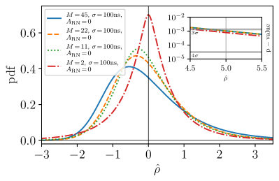
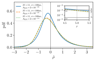
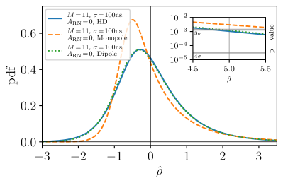
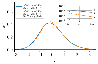
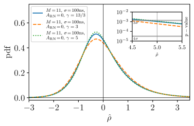
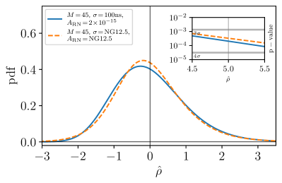
Figure 1 shows various GX2 distributions constructed from the parameters defining some simple (fictitious) PTAs, with the spectral properties of the pulsars calculated using the pulsar spectral characterization software hasasia [22]. The panels demonstrate how differences in the GW signal (spatial correlations, spectral index), noise, and timing parameters change the shape of the distribution. Note that we have not included a comparison of different WN levels because the noise power spectral densities cancel out of the numerator and denominator of $\tilde{\mathbf{Q}}$, which defines the GX2 distribution.

The interplay of the parameters makes it difficult to predict exactly what the distribution will look like. However the trends for any individual parameter follow the simple rule that as the sensitivity of the PTA is increased, the tail of the GX2 distribution becomes smaller at larger values of $\hat{\rho}$. A few other general observations are: (i) adding sufficiently large red noise to the pulsars quickly obscures the subtle differences in the GX2 distributions, as seen in panel (b) of Figure 1, and (ii) the sky positions of the pulsars matter via the $\tilde{\mathbf{S}}_{ab}$ terms in the expression for $\hat{\rho}$.

Figure 1: Comparison of GX2 distributions when varying different PTA parameters: (a) varying the number of pulsars for fixed pulsar white noise; (b) varying the amplitude of the common-spectrum red-noise process for fixed pulsar white-noise and number of pulsars; (c) comparing distributions with different spatial correlations for fixed pulsar white noise and number of pulsars; (d) comparing distributions having a non-trivial and trivial (i.e., identity) timing model; (e) varying the spectral index of the GWB search for fixed white noise and number of pulsars; (f) comparing a set of realistic NANOGrav parameters, with a simple white-noise plus common-spectrum red-noise process. The insets show plots of the $p$-values of the various GX2 distributions as functions of $\hat{\rho}$. The gray bands show the $p$-values for traditional $3\sigma$ and $4\sigma$ detection significances based on a unit (standard normal) Gaussian distribution. Note that the 11, 22 and 45 pulsar cases all fall along the same $p$-values in (a).

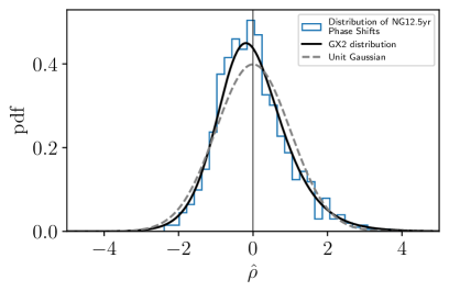
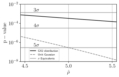
Next, we present a realistic GX2 distribution calculated using the noise and sensitivity parameters of the NANOGrav 12.5-year dataset [23, 24] to demonstrate the usefulness of an accurate analytic GX2 distribution in calculating $p$-values or false-alarm probabilities. Diagonalizing the various matrices described in Sec. III over full PTA datasets is challenging because of the length of the datasets. Nonetheless, by using the salient noise and sensitivity parameters of the NANOGrav 12.5 dataset, we obtain fairly reasonable agreement with the phase-shift method for determining the null distribution of the optimal statistic. This is illustrated in Figure 2, which compares the analytic GX2 distribution with a histogram of $\hat{\rho}$ values for 1000 different phase shifts of the NANOGrav 12.5-year data. For reference, we also show the unit (standard normal) Gaussian distribution.

By looking at the right-hand panel of Figure 2, one immediately sees the inaccuracy that would arise if the $p$-value was calculated assuming that the null distribution was Gaussian. Table 1 gives the $p$-values for $\hat{\rho}=5$ and $\hat{\rho}=1.3$ calculated using the analytic form of the GX2 distribution, the Gaussian distribution, and from phase-shifts and sky scrambles of the NANOGrav 12.5-yr data, the latter as described in [16, 17, 5]. (The value $\hat{\rho}=1.3$ is what was measured in the NANOGrav 12.5-year dataset.) While the agreement between the various methods is reasonable for the lower value of $\hat{\rho}$, assuming that the null distribution is Gaussian for $\hat{\rho}=5$ leads to a $p$-value that is a more than 1000 times smaller than it should be.

$\quad\hat{\rho}\quad$	Analytic GX2	Gaussian	Phase Shifts	Sky Scrambles
5	$3.3\times 10^{-4}$	$2.87\times 10^{-7}$	—	—
1.3	$0.0983$	$0.0951$	0.091 [5]	0.082 [5]

Table 1: $p$ -values calculated using various methods in the context of the NANOGrav 12.5-year dataset.

Figure 2: Comparison of various distributions of the OS signal-to-noise ratio $\hat{\rho}$ in the absence of GW-induced spatial correlations. Shown are: (i) an empirical null distribution for the NANOGrav 12.5-yr data, obtained from performing 1000 phase shifts (blue histogram), (ii) the analytic GX2 distribution (black solid line), and (iii) best-fit (standard normal) Gaussian distribution (gray dashed line). The right panel is a plot of the $p$ -value as a function of $\hat{\rho}$. The phase shifts don’t show up in the right-panel plot out to these large values of $\hat{\rho}$.

V Discussion

We have demonstrated that a generalized chi-squared (GX2) distribution is the correct analytical distribution for the optimal cross-correlation statistic (OS) used for analyzing PTA datasets. Although we focused on the null distribution of the OS signal-to-noise ratio $\hat{\rho}$ for this paper, our analyses in Secs. III.1 and III.2 were sufficiently general to show that GX2 distributions also apply to the optimal estimator of the squared-amplitude $\hat{A}_{\rm gw}^{2}$ and pulsar-pair cross-correlations $\hat{\rho}_{ab}$ in the presence of a signal.

We applied the general formalism to calculate the GX2 distribution for $\hat{\rho}$ using parameters appropriate for NANOGrav’s 12.5-yr dataset, and showed that it agreed quite well with the empirical null distribution that was obtained by phase-shifting the NANOGrav data. We also calculated the GX2 distribution for several different sets of simulated data, in the absence of a GWB cross-correlation, varying in turn the number of pulsars, the relative contribution of red and white noise, etc., to see how these affected the shape of the resulting distributions.

Generically, the GX2 distributions we obtained differed from the best-fit (standard normal) Gaussian distribution by having a mode less than their mean and having “fatter” tails at high values of the statistic. (Both distributions have zero mean and unit variance for the null distribution case.) The fatter tails are especially important when calculating $p$-values for the null distribution, which is needed to assess the statistical significance of a possible detection.

As mentioned in Sec. IV, constructing the quadratic form for the GX2 distribution—which requires solving for the eigenvectors of large matrices—is challenging for realistic data. Using the full NANOGrav 12.5-year dataset would require solving the eigenvalue problem for an $N=410064$ dimensional matrix twice. An additional complication is that the detailed dispersion-measure-variation (DMX) model that NANOGrav uses [25] has a large effect on the transmission function of the pulsars [21, 26]. This shows up in the timing model fit, which enters the quadratic form via the $G$-matrix, e.g., $\mathbf{r}_{a}=\mathbf{G}_{a}^{T}\boldsymbol{\delta}\mathbf{t}_{a}$.

As such, the key to constructing a valid GX2 distribution for a realistic PTA dataset is to find a reduced set of parameters that faithfully describes the spectral properties of the PTA pulsars and the corresponding timing model of the array. We used hasasia to calculate the spectra for all of the NG12.5 pulsars, using their full datasets [21]. The noise power spectral density (from the spectrum) and red noise parameters (from the Bayesian noise analyses) were then used to construct shorter datasets with similar properties, including the broadband effect of the DMX model. Spectra of these simulated datasets were taken to iteratively find the correct effective level of the white noise power spectral density to inject into the pulsars to match the spectra from the full datasets.

This process proved expeditious to obtain a fairly accurate realization of a GX2 distribution on a modest laptop. But it is computationally inefficient for generating GX2 distributions for several different choices of noise parameters, for example. Fortunately, PTA calculations are usually carried out using a rank-reduced formalism [27] that drastically reduces the size of matrices dealt with in the analysis. This reduced representation of the data alleviates the main problem discussed previously. For example, we are currently developing techniques to use a frequency-domain implementation of the optimal statistic to speed up the calculation, taking advantage of the rank-reduced matrix, which is only $2N_{\rm freq}\times 2N_{\rm freq}$, as opposed to $N_{\rm TOA}\times N_{\rm TOA}$. But we leave that discussion for future work.

An alternative to using noise estimates from a previous Bayesian inference run to calculate the optimal statistic is to marginalize over the noise parameters. As described in [12], marginalizing over the red noise parameters tends to remove biases that would otherwise exist due to correlations between the noise estimates and the timing residual data used to construct the optimal statistic. For the analyses described in this paper, we used maximum likelihood estimates of noise parameters from a Bayesian analysis to construct the quadratic forms needed for calculating the GX2 distributions. We did not investigate any source of bias that might have been introduced by using noise estimates as opposed to noise marginalization. But we are currently investigating the possibility of marginalizing over the noise for future uses of the GX2 distributions.

Finally, optimal cross-correlation statistics are also used when analyzing data from ground-based GW detectors like Advanced LIGO, Virgo, and KAGRA. However, for this case, the optimal statistics are well-described by Gaussian distributions, so GX2 distributions are not needed. This is because the data from pairs of detectors are analyzed in roughly 100-sec segments (to account for potential non-stationarities in the detector noise power) and then averaged together over $\gtrsim 10^{5}$ such segments, corresponding to a typical year-long observation. The cross-correlation estimates of the amplitude of the GWB for each 100-sec segement are GX2 distributed. But the final averaged optimal-statistic value (inverse-noise-weighted by the variance of the individual estimates) is well-described by a Gaussian distribution due to the central-limit theorem.

Appendix A Empirical tail fitting and extrapolation

The GX2 is the analytic null distribution for the optimal statistic, but it depends upon specific characteristics of the dataset e.g., white noise and red noise parameters. In the case of red noise, a Bayesian analysis is used to obtain a posterior distribution on the amplitude and spectral index, and using different draws from that posterior to calculate the GX2 changes the resulting distribution. Choosing the best parameters to use requires care and potentially comparison with empirical distributions. In this appendix we introduce a technique that can be used in the interim. In situations where we need to evaluate the null distribution in a place where we have few empirical simulations, but we don’t yet have the full GX2 method, we can empirically fit the tail of the empirical simulations with an exponential function. This method has been used to extrapolate the tail of the null distribution in e.g., searches for GWs from rapidly rotating neutron stars [28]. The uncertainty on the fit parameters can then be used to bound our estimate of the $p$-value or false alarm probability.

We begin by choosing a point beyond which $p(\hat{\rho})$ looks like an exponential. This choice is arbitrary, but the procedure can be done using several choices, picking the one that looks most reasonable. We call this value $\hat{\rho}_{\mathrm{tail}}$. Therefore, for $\hat{\rho}>\hat{\rho}_{\mathrm{tail}}$, we have

$$p(\hat{\rho}|\hat{\rho}>\hat{\rho}_{\mathrm{tail}})=\lambda\exp\left[-\lambda\left(\hat{\rho}-\hat{\rho}_{\mathrm{tail}}\right)\right]\,.$$ (49)

The shape parameter $\lambda$ is a free parameter that we fit using the values in the tail of the empirical distribution. Since there is only a single free parameter, we can fit this using a brute-force Bayesian approach, with a uniform prior on $\lambda$

$$p[\lambda|\left\{\hat{\rho}\right\}_{i=1}^{N_{\mathrm{tail}}}]=\frac{1}{\lambda_{\mathrm{max}}}\lambda^{N_{\mathrm{tail}}}\exp{\left[-\lambda\sum_{i=1}^{N_{\mathrm{tail}}}\left(\hat{\rho}_{i}-\hat{\rho}_{\mathrm{tail}}\right)\right]}\,,$$ (50)

where $N_{\mathrm{tail}}$ is the number of empirical distribution values satisfying $\hat{\rho}_{i}>\hat{\rho}_{\mathrm{tail}}$, and $\lambda_{\mathrm{max}}$ is the upper bound on the uniform prior on $\lambda$. In this notation, $\{\hat{\rho}_{i}\}_{i=1}^{N_{\textrm{tail}}}$ denotes the set of empirical distribution results that populate the tail.

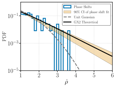
The posterior on $\lambda$ can then be used to quantify the uncertainty in the tail of the distribution on $\hat{\rho}$. We show an example of fits to the tail of the empirical distribution in Figure 3 using 300 different draws from the posterior on $\lambda$ (the 90% credible interval is shown in orange), along with the GX2 estimate (black line), and the empirical distribution (blue histogram). The blue histogram uses the phase shifts from the NANOGrav 12.5-year analysis that were used to generate Figure 2. For the sake of comparison we also include the best-fit Gaussian PDF (grey dashed), which clearly underestimates $p(\hat{\rho})$ in the tail. The exponential fit agrees with the GX2 estimate out to $\hat{\rho}=6$, indicating it can be effectively used to extrapolate the tail and still be consistent with the analytic distribution. We can also quantify the uncertainty in the tails of the empirical distribution due to having a small number of points in the tail of the empirical distribution.

Figure 3: Comparison of GX2 fit to empirical phase shifts and tail fitting procedure. Left: 90% credible interval of fit (orange) to the empirical PDF (blue). The theoretical distribution from the GX2 distribution is shown in black. Right: The same but for the $p$-value $(1-{\rm CDF})$. In both cases we can see that fitting the empirical distribution from phase shifts with an exponential gives a reasonable approximation of the GX2 in the region in which we are interested.

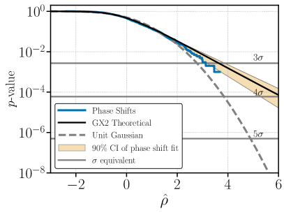
Once we have a fit for $p(\hat{\rho})$, we can analytically calculate the cumulative distribution function (CDF), $p(\hat{\rho}<\rho)$, which can be used to estimate the false alarm probability. The CDF is given by

$$p(\hat{\rho}<\rho|\lambda)=\begin{cases}\frac{1}{N}\sum_{i=1}^{N}\mathbbm{1}_{\hat{\rho}_{i}\leq\rho}&\rho\leq\hat{\rho}_{\mathrm{tail}}\,,\\[20.00003pt] \frac{1}{N}\sum_{i=1}^{N}\mathbbm{1}_{\hat{\rho}_{i}\leq\hat{\rho}_{\mathrm{tail}}}+\mathcal{N}\left(1-e^{-\lambda(\rho-\hat{\rho}_{\mathrm{tail}})}\right)&\rho>\hat{\rho}_{\mathrm{tail}}\,,\end{cases}$$ (51)

where $\mathbbm{1}$ is the indicator function that equals 1 if the subscript condition is met and equals zero otherwise. In this expression, $N$ is the total number of empirical trials and $\hat{\rho}_{i}$ is now any one of those $N$ trials (as opposed to being taken only from the tail). The normalization factor $\mathcal{N}$ is chosen such that the CDF evaluates to 1 at infinity.

References

- Siemens et al. [2013] Xavier Siemens, Justin Ellis, Fredrick Jenet, and Joseph D Romano, “The stochastic background: scaling laws and time to detection for pulsar timing arrays,” Classical and Quantum Gravity 30, 224015 (2013).
- Taylor et al. [2016a] S. R. Taylor, M. Vallisneri, J. A. Ellis, C. M. F. Mingarelli, T. J. W. Lazio, and R. van Haasteren, “Are We There Yet? Time to Detection of Nanohertz Gravitational Waves Based on Pulsar-timing Array Limits,” ApJ 819, L6 (2016a), arXiv:1511.05564 [astro-ph.IM] .
- Pol et al. [2021] Nihan S. Pol, Stephen R. Taylor, Luke Zoltan Kelley, Sarah J. Vigeland, Joseph Simon, Siyuan Chen, Zaven Arzoumanian, Paul T. Baker, Bence Bécsy, Adam Brazier, Paul R. Brook, Sarah Burke-Spolaor, Shami Chatterjee, James M. Cordes, Neil J. Cornish, Fronefield Crawford, H. Thankful Cromartie, Megan E. Decesar, Paul B. Demorest, Timothy Dolch, Elizabeth C. Ferrara, William Fiore, Emmanuel Fonseca, Nathan Garver-Daniels, Deborah C. Good, Jeffrey S. Hazboun, Ross J. Jennings, Megan L. Jones, Andrew R. Kaiser, David L. Kaplan, Joey Shapiro Key, Michael T. Lam, T. Joseph W. Lazio, Jing Luo, Ryan S. Lynch, Dustin R. Madison, Alexander McEwen, Maura A. McLaughlin, Chiara M. F. Mingarelli, Cherry Ng, David J. Nice, Timothy T. Pennucci, Scott M. Ransom, Paul S. Ray, Brent J. Shapiro-Albert, Xavier Siemens, Ingrid H. Stairs, Daniel R. Stinebring, Joseph K. Swiggum, Michele Vallisneri, Haley Wahl, Caitlin A. Witt, and Nanograv Collaboration, “Astrophysics Milestones for Pulsar Timing Array Gravitational-wave Detection,” ApJ 911, L34 (2021), arXiv:2010.11950 [astro-ph.HE] .
- Ransom et al. [2019] Scott Ransom, A. Brazier, S. Chatterjee, T. Cohen, J. M. Cordes, M. E. DeCesar, P. B. Demorest, J. S. Hazboun, M. T. Lam, R. S. Lynch, M. A. McLaughlin, S. M. Ransom, X. Siemens, S. R. Taylor, and S. J. Vigeland, “The NANOGrav Program for Gravitational Waves and Fundamental Physics,” in BAAS, Vol. 51 (2019) p. 195, arXiv:1908.05356 [astro-ph.IM] .
- Arzoumanian et al. [2020] Zaven Arzoumanian, Paul T. Baker, Harsha Blumer, Bence Becsy, Adam Brazier, Paul R. Brook, Sarah Burke-Spolaor, Shami Chatterjee, Siyuan Chen, James M. Cordes, Neil J. Cornish, Fronefield Crawford, H. Thankful Cromartie, Megan E. DeCesar, Paul B. Demorest, Timothy Dolch, Justin A. Ellis, Elizabeth C. Ferrara, William Fiore, Emmanuel Fonseca, Nathan Garver-Daniels, Peter A. Gentile, Deborah C. Good, Jeffrey S. Hazboun, A. Miguel Holgado, Kristina Islo, Ross J. Jennings, Megan L. Jones, Andrew R. Kaiser, David L. Kaplan, Luke Zoltan Kelley, Joey Shapiro Key, Nima Laal, Michael T. Lam, T. Joseph W. Lazio, Duncan R. Lorimer, Jing Luo, Ryan S. Lynch, Dustin R. Madison, Maura A. McLaughlin, Chiara M. F. Mingarelli, Cherry Ng, David J. Nice, Timothy T. Pennucci, Nihan S. Pol, Scott M. Ransom, Paul S. Ray, Brent J. Shapiro-Albert, Xavier Siemens, Joseph Simon, Renee Spiewak, Ingrid H. Stairs, Daniel R. Stinebring, Kevin Stovall, Jerry P. Sun, Joseph K. Swiggum, Stephen R. Taylor, Jacob E. Turner, Michele Vallisneri, Sarah J. Vigeland, and Caitlin A. Witt, “The NANOGrav 12.5-year Data Set: Search For An Isotropic Stochastic Gravitational-Wave Background,” (2020), arXiv:2009.04496 [astro-ph.HE] .
- Goncharov et al. [2021] Boris Goncharov et al., “On the Evidence for a Common-spectrum Process in the Search for the Nanohertz Gravitational-wave Background with the Parkes Pulsar Timing Array,” Astrophys. J. Lett. 917, L19 (2021), arXiv:2107.12112 [astro-ph.HE] .
- Chen et al. [2021] S. Chen et al., “Common-red-signal analysis with 24-yr high-precision timing of the European Pulsar Timing Array: inferences in the stochastic gravitational-wave background search,” Mon. Not. Roy. Astron. Soc. 508, 4970–4993 (2021), arXiv:2110.13184 [astro-ph.HE] .
- Antoniadis et al. [2022] J. Antoniadis et al., “The International Pulsar Timing Array second data release: Search for an isotropic gravitational wave background,” Mon. Not. Roy. Astron. Soc. 510, 4873–4887 (2022), arXiv:2201.03980 [astro-ph.HE] .
- Hellings and Downs [1983] R. W. Hellings and G. S. Downs, “Upper limits on the isotropic gravitational radiation background from pulsar timing analysis,” Astrophys. J. Lett. 265, L39–L42 (1983).
- Anholm et al. [2009] M. Anholm, S. Ballmer, J. D. E. Creighton, L. R. Price, and X. Siemens, “Optimal strategies for gravitational wave stochastic background searches in pulsar timing data,” Phys. Rev. D 79, 084030 (2009), arXiv:0809.0701 [gr-qc] .
- Chamberlin et al. [2015] S. J. Chamberlin, J. D. E. Creighton, X. Siemens, P. Demorest, J. Ellis, L. R. Price, and J. D. Romano, “Time-domain implementation of the optimal cross-correlation statistic for stochastic gravitational-wave background searches in pulsar timing data,” Phys. Rev. D 91, 044048 (2015), arXiv:1410.8256 [astro-ph.IM] .
- Vigeland et al. [2018] Sarah J. Vigeland, Kristina Islo, Stephen R. Taylor, and Justin A. Ellis, “Noise-marginalized optimal statistic: A robust hybrid frequentist-bayesian statistic for the stochastic gravitational-wave background in pulsar timing arrays,” Phys. Rev. D 98, 044003 (2018).
- Romano and Cornish [2017] Joseph D. Romano and Neil. J. Cornish, “Detection methods for stochastic gravitational-wave backgrounds: a unified treatment,” Living Reviews in Relativity 20, 2 (2017).
- Das and Geisler [2021] Abhranil Das and Wilson S Geisler, “A method to integrate and classify normal distributions,” Journal of Vision 21, 1–17 (2021).
- Cordes and Shannon [2012] J. M. Cordes and R. M. Shannon, “Minimum Requirements for Detecting a Stochastic Gravitational Wave Background Using Pulsars,” ApJ 750, 89 (2012), arXiv:1106.4047 [astro-ph.GA] .
- Taylor et al. [2016b] S. R. Taylor, L. Lentati, S. Babak, P. Brem, J. R. Gair, A. Sesana, and A. Vecchio, “All correlations must die: Assessing the significance of a stochastic gravitational-wave background in pulsar-timing arrays,” ArXiv e-prints (2016b), arXiv:1606.09180 [astro-ph.IM] .
- Cornish and Sampson [2016] N. J. Cornish and L. Sampson, “Towards robust gravitational wave detection with pulsar timing arrays,” Phys. Rev. D 93, 104047 (2016), arXiv:1512.06829 [gr-qc] .
- van Haasteren and Levin [2013] Rutger van Haasteren and Yuri Levin, “Understanding and analysing time-correlated stochastic signals in pulsar timing,” MNRAS 428, 1147–1159 (2013), arXiv:1202.5932 [astro-ph.IM] .
- Lam et al. [2018] M. T. Lam, M. A. McLaughlin, J. M. Cordes, S. Chatterjee, and T. J. W. Lazio, “Optimal Frequency Ranges for Submicrosecond Precision Pulsar Timing,” ApJ 861, 12 (2018), arXiv:1710.02272 [astro-ph.HE] .
- Lam [2018] M. T. Lam, “Optimizing Pulsar Timing Array Observational Cadences for Sensitivity to Low-frequency Gravitational-wave Sources,” ApJ 868, 33 (2018), arXiv:1808.10071 [astro-ph.HE] .
- Hazboun et al. [2019] Jeffrey S. Hazboun, Joseph D. Romano, and Tristan L. Smith, “Realistic sensitivity curves for pulsar timing arrays,” Phys. Rev. D 100, 104028 (2019).
- Hazboun et al. [2019] Jeffrey Hazboun, Joseph Romano, and Tristan Smith, “Hasasia: A Python package for Pulsar Timing Array Sensitivity Curves,” The Journal of Open Source Software 4, 1775 (2019).
- Alam et al. [2020] Md F. Alam, Zaven Arzoumanian, Paul T. Baker, Harsha Blumer, Keith E. Bohler, Adam Brazier, Paul R. Brook, Sarah Burke-Spolaor, Keeisi Caballero, Richard S. Camuccio, Rachel L. Chamberlain, Shami Chatterjee, James M. Cordes, Neil J. Cornish, Fronefield Crawford, H. Thankful Cromartie, Megan E. DeCesar, Paul B. Demorest, Timothy Dolch, Justin A. Ellis, Robert D. Ferdman, Elizabeth C. Ferrara, William Fiore, Emmanuel Fonseca, Yhamil Garcia, Nathan Garver-Daniels, Peter A. Gentile, Deborah C. Good, Jordan A. Gusdorff, Daniel Halmrast, Jeffrey Hazboun, Kristina Islo, Ross J. Jennings, Cody Jessup, Megan L. Jones, Andrew R. Kaiser, David L. Kaplan, Luke Zoltan Kelley, Joey Shapiro Key, Michael T. Lam, T. Joseph W. Lazio, Duncan R. Lorimer, Jing Luo, Ryan S. Lynch, Dustin Madison, Kaleb Maraccini, Maura A. McLaughlin, Chiara M. F. Mingarelli, Cherry Ng, Benjamin M. X. Nguyen, David J. Nice, Timothy T. Pennucci, Nihan S. Pol, Joshua Ramette, Scott M. Ransom, Paul S. Ray, Brent J. Shapiro-Albert, Xavier Siemens, Joseph Simon, Renee Spiewak, Ingrid H. Stairs, Daniel R. Stinebring, Kevin Stovall, Joseph K. Swiggum, Stephen R. Taylor, Michael Tripepi, Michele Vallisneri, Sarah J. Vigeland, Caitlin A. Witt, and Weiwei Zhu, “The NANOGrav 12.5-year Data Set: Observations and Narrowband Timing of 47 Millisecond Pulsars,” ApJS 252, 1 (2020), arXiv:2005.06490 [astro-ph.HE] .
- Arzoumanian et al. [2020] Zaven Arzoumanian, Paul T. Baker, Harsha Blumer, Bence Bécsy, Adam Brazier, Paul R. Brook, Sarah Burke-Spolaor, Shami Chatterjee, Siyuan Chen, James M. Cordes, Neil J. Cornish, Fronefield Crawford, H. Thankful Cromartie, Megan E. Decesar, Paul B. Demorest, Timothy Dolch, Justin A. Ellis, Elizabeth C. Ferrara, William Fiore, Emmanuel Fonseca, Nathan Garver-Daniels, Peter A. Gentile, Deborah C. Good, Jeffrey S. Hazboun, A. Miguel Holgado, Kristina Islo, Ross J. Jennings, Megan L. Jones, Andrew R. Kaiser, David L. Kaplan, Luke Zoltan Kelley, Joey Shapiro Key, Nima Laal, Michael T. Lam, T. Joseph W. Lazio, Duncan R. Lorimer, Jing Luo, Ryan S. Lynch, Dustin R. Madison, Maura A. McLaughlin, Chiara M. F. Mingarelli, Cherry Ng, David J. Nice, Timothy T. Pennucci, Nihan S. Pol, Scott M. Ransom, Paul S. Ray, Brent J. Shapiro-Albert, Xavier Siemens, Joseph Simon, Renée Spiewak, Ingrid H. Stairs, Daniel R. Stinebring, Kevin Stovall, Jerry P. Sun, Joseph K. Swiggum, Stephen R. Taylor, Jacob E. Turner, Michele Vallisneri, Sarah J. Vigeland, Caitlin A. Witt, and Nanograv Collaboration, “The NANOGrav 12.5 yr Data Set: Search for an Isotropic Stochastic Gravitational-wave Background,” ApJ 905, L34 (2020), arXiv:2009.04496 [astro-ph.HE] .
- The NANOGrav Collaboration et al. [2015] The NANOGrav Collaboration, Z. Arzoumanian, A. Brazier, S. Burke-Spolaor, S. Chamberlin, S. Chatterjee, B. Christy, J. M. Cordes, N. Cornish, K. Crowter, P. B. Demorest, T. Dolch, J. A. Ellis, R. D. Ferdman, E. Fonseca, N. Garver-Daniels, M. E. Gonzalez, F. A. Jenet, G. Jones, M. L. Jones, V. M. Kaspi, M. Koop, M. T. Lam, T. J. W. Lazio, L. Levin, A. N. Lommen, D. R. Lorimer, J. Luo, R. S. Lynch, D. Madison, M. A. McLaughlin, S. T. McWilliams, D. J. Nice, N. Palliyaguru, T. T. Pennucci, S. M. Ransom, X. Siemens, I. H. Stairs, D. R. Stinebring, K. Stovall, J. K. Swiggum, M. Vallisneri, R. van Haasteren, Y. Wang, and W. Zhu, “The NANOGrav Nine-year Data Set: Observations, Arrival Time Measurements, and Analysis of 37 Millisecond Pulsars,” ApJ 813, 65 (2015), arXiv:1505.07540 [astro-ph.IM] .
- Demorest [2007] Paul B. Demorest, Measuring the gravitational wave background using precision pulsar timing, Ph.D. thesis, University of California, Berkeley (2007).
- van Haasteren and Vallisneri [2015] R. van Haasteren and M. Vallisneri, “Low-rank approximations for large stationary covariance matrices, as used in the Bayesian and generalized-least-squares analysis of pulsar-timing data,” MNRAS 446, 1170–1174 (2015), arXiv:1407.6710 [astro-ph.IM] .
- Abbott et al. [2022] R. Abbott, T. D. Abbott, F. Acernese, K. Ackley, C. Adams, N. Adhikari, R. X. Adhikari, V. B. Adya, C. Affeldt, D. Agarwal, and et al., “Search for continuous gravitational waves from 20 accreting millisecond x-ray pulsars in O3 LIGO data,” Phys. Rev. D 105, 022002 (2022), arXiv:2109.09255 [astro-ph.HE] .