Self-similar growth of Bose stars

Abstract

We analytically solve the problem of Bose star growth in the bath of gravitationally interacting particles. We find that after nucleation of this object the bath is described by a self-similar solution of kinetic equation. Together with the conservation laws, this fixes mass evolution of the Bose star. Our theory explains, in particular, the slowdown of the star growth at a certain “core-halo” mass, but also predicts formation of heavier and lighter objects in magistral dark matter models. The developed “adiabatic” approach to self-similarity may be of interest for kinetic theory in general.

1. Introduction.

Gravitationally bound blobs of Bose-Einstein condensate Ruffini and Bonazzola (1969); *Tkachev:1986tr — Bose stars — have regained a lot of attention recently. This is because they are abundant in models with light dark matter Ringwald, Rosenberg, and Rybka (2022); *Niemeyer:2019aqm consisting, e.g., of “fuzzy” bosons or QCD axions. In those two cases, the Bose stars are called “solitonic galaxy cores” Schive, Chiueh, and Broadhurst (2014) and “axion stars” Ringwald, Rosenberg, and Rybka (2022); *Niemeyer:2019aqm, respectively. Typically, the self-couplings of light dark matter particles are tiny and can be ignored. But their phase-space density is so large Tkachev (1991) that thermalization can occur inside the smallest cosmological structures via universal gravitational interactions Levkov, Panin, and Tkachev (2018). This makes the Bose star appear in the center of every such structure Schive, Chiueh, and Broadhurst (2014); Levkov, Panin, and Tkachev (2018); Eggemeier and Niemeyer (2019) in kinetic time.

The question is, how do the newborn Bose stars grow? Lattice simulations show that their masses increase at first as $M_{bs}\propto t^{1/2}$ Levkov, Panin, and Tkachev (2018) and then slow down Eggemeier and Niemeyer (2019). But the numerical results on the late-time behavior are conflicting: $M_{bs}\propto t^{1/8}$ in Eggemeier and Niemeyer (2019); Chen et al. (2021) and $t^{1/4}$ in Chan, Sibiryakov, and Xue .

In this Letter, we for the first time show  that Bose-Einstein condensation of dark matter via gravitational (long-range) scattering is described by self-similar solutions of kinetic equation. Computing the condensation flux onto the Bose star, we analytically obtain its growth law. The star mass is not a simple power of time, but can be piecewise approximated by all of the behaviors above.

2. A crucial observation.

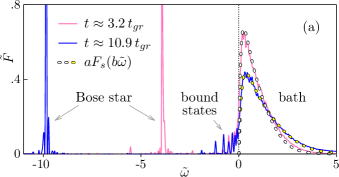
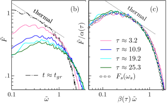
Figure 1: Simulation of Eq. (1) with $M=50\,p_{0}/m^{2}G$ and $L=60/p_{0}$. (a) Spectra (2) at two moments of time (solid lines). (b) Bath spectra (${\omega>0}$) at large times and (c) their self-similar transformation (3) with ${D=2.8}$. Figure (b) includes $t\approx t_{gr}$ graph (dash-dotted). Chain points in Figs. (a), (c) show the solution of Eq. (5) with $D=2.8$ and the source; see Supplemental Material C (SM-C) for parameters.

Consider a cloud of nonrelativistic dark matter bosons inside the smallest cosmological structure: a minicluster of axions Kolb and Tkachev (1993); *Kolb:1993hw; *Vaquero:2018tib; *Buschmann:2019icd; *Eggemeier:2019khm; *Ellis:2020gtq or a galaxy halo of “fuzzy” dark matter. At small particle masses $m$ the occupation numbers are so large that the bosons are described by a random classical field $\psi(t,\,\boldsymbol{x})$ evolving in its own gravitational potential $U(t,\,\boldsymbol{x})$,

$$i\partial_{t}\psi=-\Delta\psi/2m+mU\psi\,,$$ (1)

$$\Delta U=4\pi G\,(m|\psi|^{2}-\bar{\rho})\,,$$

where $\bar{\rho}\equiv M/L^{3}$ is the mean density and $M$ is the total mass. For simplicity, we approximate the structure with periodic box of size $L$.

We solve Eqs. (1) using a stable 3D code of Ref. Levkov, Panin, and Tkachev (2018). The starting point of this evolution is a virial equilibrium, i.e. Gaussian-distributed field with Fourier image $|\psi_{\boldsymbol{p}}|^{2}\propto M\mathrm{e}^{-\boldsymbol{p}^{2}/p_{0}^{2}}$ and random phases $\arg\psi_{\boldsymbol{p}}$; here $\omega_{0}\equiv p_{0}^{2}/2m$ is the typical particle energy . We study mass distribution $F(t,\,\omega)=dM/d\omega$ of bosons over energies $\omega$. It is given by time Fourier transform Levkov, Panin, and Tkachev (2018):

$$F=m\int\frac{dt^{\prime}}{2\pi}\,d^{3}\boldsymbol{x}\,\psi^{*}(t,\boldsymbol{x})\psi(t+t^{\prime},\boldsymbol{x})\,\mathrm{e}^{i\omega t^{\prime}-t^{\prime 2}/\Delta t^{2}}\,,$$ (2)

where $\Delta t^{-1}\ll\omega_{0}$ is the energy resolution. In the isotropic homogeneous case, this function is related to the usual phase-space density $f(p)$ as $F=L^{3}m^{2}pf/2\pi^{2}$ with $\omega=p^{2}/2m$. Below we exploit dimensionless units: $\tilde{F}(t,\,\tilde{\omega})\equiv 2\omega_{0}F/M$ and $\tilde{\omega}\equiv\omega/2\omega_{0}$.

Our ensemble has large occupation numbers and hence thermalizes into a Bose-Einstein condensate. This is seen in simulations Levkov, Panin, and Tkachev (2018) as phase transition at a kinetic time $t=t_{gr}\equiv 2b\sqrt{2}\,\omega_{0}^{3}/[3\pi^{3}{G^{2}\bar{\rho}^{2}\ln(p_{0}L)}]$, where ${b\approx 0.9}$ for the Gaussian initial distribution. Namely, after $t_{gr}$ the spectrum $F(t,\,\omega)$ develops a narrow peak at $\omega\approx\omega_{bs}<0$ moving with time to lower energies; see Fig. 1(a) and the video Simulation movie for $M=20\,p_{0}/m^{2}G$ and $L=40/p_{0}$; cf. Figs. , . Four panels show time evolutions of $\tilde{F}$$,therescaleddistribution(\ref{eq:ab}),particledensity$—ψ(x)—^2$,and$M_bs$(toptobottom,lefttoright)$(2023) (~ω). The peak is a Bose star Ruffini and Bonazzola (1969); *Tkachev:1986tr; Ringwald, Rosenberg, and Rybka (2022); *Niemeyer:2019aqm: a condensate of particles occupying a single — ground — level $\omega_{bs}$ in the collective gravitational well $U$. Once the Bose star appears, the ensemble mass $M=M_{bs}+M_{e}+M_{b}$ divides between this object ($M_{bs}$), excited bound states in its gravitational field ($M_{e}$), and the “bath” of particles with $\omega>0$ ($M_{b}$). The conditions for condensation are still satisfied, so $M_{*}$ grows at $t>t_{gr}$.

Below we measure time in kinetic intervals $\tau\equiv t/t_{gr}$ and compute $M_{i}$ by integrating $F(\omega)$ over the respective regions. E.g., the “dressed star” mass is $M_{*}\equiv M_{bs}+M_{e}=\int_{\omega<0}F\,d\omega$, while $M_{b}$ and $M_{bs}$ are the integrals over $\omega>0$ and $\omega\approx\omega_{bs}$, respectively.

Now, we make an important observation. Consider the $\omega>0$ spectrum, i.e. the “bath”. It changes a lot after the Bose star formation, cf.  the graphs with different $\tau$ in Fig. 1(b). The same graphs, however, coincide in Fig. 1(c) after time-dependent rescaling of $F$ and $\omega$:

$$\tilde{F}(t,\,\tilde{\omega})=\alpha F_{s}(\beta\tilde{\omega})\,,\quad\alpha=\tau^{-1/D}\,,\quad\beta=\tau^{2/D-1}\,,$$ (3)

where $D=2.8$. This means that the bath is self-similar and can be fully described by a function $F_{s}(\omega_{s})$. Below we demonstrate that Eq. (3) is an attractor solution: kinetic evolution generically approaches it at large $t$.

It is worth noting that Bose star formation can be perceived as a second-order critical phenomenon. First, its order parameter $M_{bs}(t)$ grows from zero at ${t\geq t_{gr}}$. Second, the bath spectrum has thermal small-$\omega$ tail ${F\propto\omega^{-1/2}}$ at $t\approx t_{gr}$, see Fig. 1(b). In Supplemental Material A (SM-A) we show that this entails power-law field correlators at large distances. The thermal parts remain in the self-similar spectra at $t>t_{gr}$, cf. Fig. 1(c).

3. Self-similar attractor.

Let us ignore the effect of Bose star gravitational field on the bath. Then evolution of $F(t,\,\omega)$ at $\omega>0$ is governed by a homogeneous and isotropic kinetic equation Lifshitz and Pitaevskii (2012); *2013PhyU...56...49Z; *Skipp:2020xcc; Levkov, Panin, and Tkachev (2018)

$$\partial_{\tau}\tilde{F}=\mathrm{St}\,\tilde{F}\,,$$ (4)

where $\mathrm{St}\,\tilde{F}$ is the Landau scattering integral — functional of $\tilde{F}(\tilde{\omega})$ at given $\tau$, see its explicit form in Levkov, Panin, and Tkachev (2018) and SM-B.

Dramatically, the ansatz (3) passes through Eq. (4) at any $D$ leaving a one-dimensional equation for the profile,

$$(2/D-1)\,(\omega_{s}\partial_{\omega_{s}}F_{s})-F_{s}/D=\mathrm{St}\,F_{s}\,,$$ (5)

This is guaranteed by the scaling ${\mathrm{St}\,\tilde{F}=\alpha^{3}\beta\,\mathrm{St}\,F_{s}}$ reflecting long-range nature of gravitational scattering, see Levkov, Panin, and Tkachev (2018) and SM-B. The scaling is generic: one can find it even using the estimate $\mathrm{St}\,F\sim{F/t_{gr}}$.

On the other hand, Eq. (3) is not a solution if the bath is isolated. Indeed, self-similarity gives time-dependent mass ${M_{b}\propto\tau^{k_{M}}}$ and energy ${E_{b}\propto\tau^{k_{E}}}$ with

$$k_{M}=1-3/D\,,\quad k_{E}=2-5/D\,,\quad 3k_{E}-5k_{M}=1\,.$$ (6)

This contradicts to the conservation laws.

But the ongoing condensation radically changes the boundary conditions for the bath. Indeed, the bath bosons may scatter, loose energy, and append either to the Bose star or to one of its bound states at $\omega<0$. Besides, with time the star gravitational well grows deeper and adiabatically drags low-energy particles to $\omega<0$. Both mechanisms absorb bosons with $\omega\approx 0$, since gravitational scattering is more effective at low transfers $\Delta\omega\ll\omega_{0}$ Lifshitz and Pitaevskii (2012); *2013PhyU...56...49Z. This heats the remaining ensemble due to energy conservation. As a result, the bath has decreasing $M_{b}$ and growing $E_{b}$, i.e. $5/2<D<3$ in Eq. (6).

To account for condensation in Eq. (5), we impose a condition of finite particle flux at ${\omega_{s}\approx 0}$ and add an energy source $\mathrm{St}\,F_{s}\to\mathrm{St}\,F_{s}+J_{s}(\omega_{s})$ to the right-hand side. This gives a family of solutions at $D\geq 5/2$; see SM-C for details. The solution $F_{s}(\omega_{s})$ with $D=2.8$ and properly selected $J_{s}(\omega_{s})$ is shown in Figs. 1(a), (c) by chain points. Having almost constant condensation flux at low $\omega_{s}$, it nevertheless considerably differs from the power-law Kolmogorov cascades Zakharov, L’vov, and Falkovich (2012).

It is crucial that the self-similar solutions (3) are attractors of kinetic evolution. This property is apparent in Fig. 1(c), but we confirm it explicitly in SM-D by solving the full kinetic equation (4) with time-dependent source $\tilde{J}(\tau,\,\tilde{\omega})$. Even if $\tilde{J}$ is essentially non self-similar, the solution $\tilde{F}(\tau,\,\tilde{\omega})$ approaches Eq. (3) with some $D$.

4. Growth of the Bose star.

In our problem, self-similarity of the bath is broken by the Bose star which injects energy at its own, non scale-invariant rate $J$. On the other hand, the self-similar solutions are attractors. This implies an “adiabatic” regime which was never studied before: the bath remains almost self-similar at all times, but its parameters slowly drift with time.

In the first — crude — approximation we can account for time dependence of $D=D(\tau)$. Define $k_{M}(\tau)\equiv d\ln M_{b}/d\ln\tau$ and $k_{E}(\tau)\equiv d\ln E_{b}/d\ln\tau$. We assume that they satisfy the self-similar law (6), ${3k_{E}-5k_{M}\approx 1}$, if they change slowly. Then the conservation laws $M_{b}=M-M_{*}$ and $E_{b}=E-E_{*}$ give $d\!\ln\tau\approx 3d\!\ln(E-E_{*})-5d\!\ln(M-M_{*})$ or, integrating,

$$(1-E_{*}/E)^{3}(1-M_{*}/M)^{-5}\approx(\tau-\tau_{i})/\tau_{*}\,,$$ (7)

where $\tau_{*}$ is an integration constant, $M_{*}$ and $E_{*}$ are the parameters of the “dressed” star, and we recalled the time translations $\tau\to\tau-\tau_{i}$ .

To extract the Bose star mass evolution from Eq. (7), we estimate the contributions of the excited discrete levels at $\omega<0$. Theory suggests that large-mass condensate cannot be accumulated on those levels: it would become unstable once gravitationally self-bound Lee and Pang (1989); Dmitriev et al. (2021). Then $M_{e}<M_{bs}$. This is confirmed by our simulations: $M_{e}(t)\equiv M_{*}-M_{bs}$ is small and almost constant in Fig. 2(a) at $\tau\gtrsim 2$. Moreover, the excited levels with $\omega<0$ carry negligibly small energy in simulations as compared to the Bose star itself: $E_{*}\approx{E_{bs}=-\gamma M_{bs}^{3}}$, where $\gamma\approx 0.0542\,m^{2}G^{2}$ Dmitriev et al. (2021). Indeed, in Fig. 1(a) only the bound states with $\omega\approx 0$ are occupied. Taking $E_{*}\approx E_{bs}$  and constant $x_{e}\equiv M_{e}/M$, we obtain the growth law for $x_{bs}(\tau)\equiv M_{bs}/M$:

$$(1+x_{bs}^{3}/\epsilon^{2})^{3}(1-x_{e}-x_{bs})^{-5}\approx(\tau-\tau_{i})/\tau_{*}\,.$$ (8)

Here $\epsilon^{2}\equiv E/\gamma M^{3}$ is a combination of the total mass and energy proportional to the invariant $\Xi$ from Refs. Schwabe, Niemeyer, and Engels (2016); Mocz et al. (2017), while $M_{*}(\tau)=(x_{bs}+x_{e})M$.

Note that $\tau_{i}$, $\tau_{*}$, and $x_{e}$ in Eq. (8) are empiric fitting parameters. However, $\tau_{*}\approx(1-\tau_{i})(1-x_{e})^{5}$ is fixed by the initial condition $M_{bs}=0$ at $\tau=1$, while  $x_{e}$ is small and can be ignored, if unknown. This leaves only $\tau_{i}$ to fit; in fact, $\tau_{i}\approx-0.1$ agrees with all simulations in Fig. 2.

In Fig. 2(a) we show that the theory (8) (dashed lines) reproduces the simulation results for $M_{bs}(\tau)$ and $M_{*}(\tau)$ (solid). A significant statistical test is shown in Fig. 2(b) where we display $M_{bs}(\tau)$ for 11 simulations with $\epsilon\approx 0.074$ and $22$ simulations with $\epsilon\approx 0.186$ (solid data vs.  dashed theory). These runs have essentially different parameters and kinetic times $10^{3}\lesssim\omega_{0}t_{gr}\lesssim 3\cdot 10^{4}$. Nevertheless, their graphs in Fig. 2(b) merge into two distinct curves at two values of $\epsilon$, which agree with Eq. (8). Another strong test is performed in SM-E by considering self-interacting bosons. In this case our theory still describes numerical data, although Eq. (8) gets modified by the Bose star self-interaction energy.

For gravitationally self-bound bath, $p_{0}L\sim 5/\epsilon$. This means that kinetic approach is valid at $\epsilon\ll 1$ Levkov, Panin, and Tkachev (2018). Present-day simulations Kolb and Tkachev (1993); *Kolb:1993hw; Schive, Chiueh, and Broadhurst (2014); Vaquero, Redondo, and Stadler (2019); Buschmann, Foster, and Safdi (2020); Eggemeier et al. (2020); Ellis, Marsh, and Behrens (2021) are restricted to $\epsilon\gtrsim 0.05$, cf. Fig. 2. At these values, the Bose star growth is “adiabatic” from the start: $dk_{M,E}/d\ln(\tau-\tau_{i})<{0.03/\epsilon<1}$. At smaller $\epsilon$, adiabaticity is met at later stages.

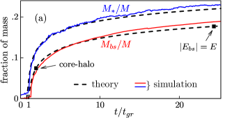
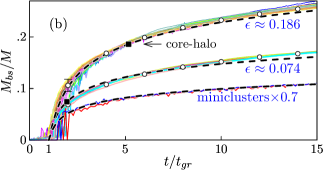
Figure 2: (a) Bose star mass $M_{bs}(t)$ and the mass of the “dressed” object $M_{*}(t)$ in the box simulation of Fig. 1 with $\epsilon\approx 0.074$. (b) Evolutions of $M_{bs}(t)$ in $11+22$ box simulations with essentially different $t_{gr}$ at two values of $\epsilon$ (two upper graphs). Numerical results are shown by solid lines, while dashed is the theory (8) with $x_{e}\approx 0.043$ and $0.021$ at $\epsilon\approx 0.074$ and $0.186$, respectively. Circles average over simulations with given $\epsilon$. The lower graph shows 2 minicluster simulations at $\epsilon\approx 0.066$ (solid lines) fitted by the theory with $x_{e}\approx 0.026$ and $\tau_{i}=-0.1$ (dashed). For visualization purposes, we rescaled the minicluster lines by $M_{bs}\to 0.7M_{bs}$.

5. Core-halo relation and beyond.

At $t\approx t_{gr}$ the energy of the baby Bose star is negligible, since ${E_{bs}\propto M_{bs}^{3}}$. Then Eq. (7) gives $M_{*}(t)\approx M\,(\tau-1)/5\tau_{*}$ — linear growth law for the “dressed” object.

During longer initial stage, the star is still small, ${E_{bs}\ll E}$, and Eq. (8) linearizes to $3x_{bs}^{3}/\epsilon^{2}+5x_{bs}\approx(\tau-1)/\tau_{*}$. Hence, at $x_{bs}\gtrsim\epsilon$ the evolution slows down to ${M_{bs}\propto t^{1/3}}$. This transition happens at $M_{bs}=\epsilon M$ when the virial velocities of the Bose star and the bath equalize, $|E_{bs}/M_{bs}|=E/M$, i.e. precisely at the “core-halo” point of Refs. Schive et al. (2014); Bar et al. (2018). The time to the slowdown is short at small $\epsilon$: $t-t_{gr}\sim 9\epsilon\,t_{gr}$. This explains, why the stars with $M_{bs}\sim\epsilon M$ form in cosmological simulations Schive, Chiueh, and Broadhurst (2014); Schive et al. (2014) and seemingly do not grow any further. In truth, the growth continues — hence scatter Schwabe, Niemeyer, and Engels (2016); Mina, Mota, and Winther (2022); *Zagorac:2022xic; Chan et al. (2022); *Nori:2020jzx in the simulation results for $M_{bs}$.

The next slowdown in Eq. (8) occurs at $E_{bs}=E$ and $M_{bs}=\epsilon^{2/3}M$. Such heavy objects were observed in some cosmological simulations Mocz et al. (2017); Mina, Mota, and Winther (2022); *Zagorac:2022xic. After this point, ${M_{bs}\propto t^{1/9}}$. Together, our laws $M_{bs}\propto t^{1/3}$ and $t^{1/9}$ agree with numerical data in  Chan, Sibiryakov, and Xue and Eggemeier and Niemeyer (2019); Chen et al. (2021).

6. Bose star growth in a halo.

Now, consider a denser gas which quickly forms a gravitationally bound halo/ minicluster under Jeans instability Levkov, Panin, and Tkachev (2018); Schwabe, Niemeyer, and Engels (2016); Chen et al. (2021). Using the distribution $F$ at $\omega<0$, we find the minicluster mass $M$, its virial energy $E_{\mathrm{mc}}<0$, and mean particle energy $\omega_{0}=-mE_{\mathrm{mc}}/M$. We also compute its central density $\bar{\rho}=\rho(0)$ and potential $U(0)$. This gives $t_{gr}$, the energy $E=E_{\mathrm{mc}}-U(0)M{>0}$ counted from the lowest level inside the halo, and $\epsilon^{2}\equiv E/\gamma M^{3}$; see details in SM-F.

With time, the minicluster gives birth to a Bose star. The growing mass of the latter is shown in Fig. 2(b) for two simulations with $\epsilon\approx 0.066$ (thin solid lines). Notably, $M_{bs}(t)$ is still described by the self-similar theory with ${\tau_{i}=-0.1}$ (dashed line), where $x_{e}$ is extracted from $F$. This coincidence strongly supports our theory, as it occurs despite the fact that Eq. (8) ignores inhomogeneity of the minicluster.

7. Discussion.

In this Letter we demonstrated that kinetics of Bose-Einstein condensation is self-similar if it is governed by gravitational (long-range) scattering. This solves a long-standing problem Zakharov and Karas’ (2013); Zakharov, L’vov, and Falkovich (2012); Skipp, L’vov, and Nazarenko (2020) with absence of Kolmogorov power-law cascades in such systems. The Bose star growth law (7), (8) was derived using the new working assumption on the “adiabaticity” of scaling exponents. This framework may be useful in other contexts.

To date, simulations of light dark matter structure formation Schive, Chiueh, and Broadhurst (2014); Schwabe and Niemeyer (2022); Li et al. cannot provide global distribution of Bose stars which are just too small. For that, one needs a theoretical input from our Eq. (8) and Refs. Kolb and Tkachev (1993); *Kolb:1993hw; *Vaquero:2018tib; *Buschmann:2019icd; *Eggemeier:2019khm; *Ellis:2020gtq, cf. Eggemeier et al. (2022); *Ellis:2022grh; *Du:2023jxh. Consider, e.g., growing Bose (axion) stars inside QCD axion miniclusters Kolb and Tkachev (1993); *Kolb:1993hw; *Vaquero:2018tib; *Buschmann:2019icd; *Eggemeier:2019khm; *Ellis:2020gtq. The latter originate from the axion overdensities $\Phi=\delta\rho/\rho|_{\mathrm{RD}}\lesssim 10$ at the radiation-dominated epoch. Equation (8) tells us that the star eats the fraction $x_{bs}\sim 0.1$ of the host minicluster in time $t\sim t_{gr}x_{bs}^{9}/\epsilon^{6}$. This time is shorter than the the age of the Universe if $\Phi\gtrsim 6\,(10\,x_{bs}m_{4})^{9/8}M_{13}^{3/4}$, where we used the estimates of Kolb and Tkachev (1994b); Levkov, Panin, and Tkachev (2018) and normalized $M_{13}\equiv M/(10^{-13}\,M_{\odot})$ and $m_{4}\equiv m/(10^{-4}\,\mbox{eV})$ to the centers of the discussed minicluster and QCD axion mass windows Kolb and Tkachev (1993); *Kolb:1993hw; *Vaquero:2018tib; *Buschmann:2019icd; *Eggemeier:2019khm; *Ellis:2020gtq; Klaer and Moore (2017); *Gorghetto:2018myk; *Gorghetto:2020qws. It is thus realistic to expect that large parts of the densest miniclusters are nowadays engulfed by their axion stars. Note that the latter may lead to spectacular observational effects, see e.g. Levkov, Panin, and Tkachev (2020); *Eby:2021ece; *Visinelli:2021uve; *Escudero:2023vgv.

The other popular model describes growth of gigantic Bose stars inside “fuzzy” dark matter galaxy halos Schive, Chiueh, and Broadhurst (2014). Such stars do not reach the “core-halo” point if the required time $\Delta t\sim 9\epsilon t_{gr}$ exceeds the age of the Universe. This happens if $m\gtrsim 6\cdot 10^{-21}\,\mbox{eV}\cdot v_{30}^{5/2}\,M_{8}^{-3/2}$, where we normalized the virial velocity $v_{30}\equiv v/(30\ \mbox{km}/\mbox{s})$ and mass $M_{8}\equiv M/(10^{8}\,M_{\odot})$ to the smallest dwarf galaxies. We see that the “fuzzy” Bose stars should be undergrown in all galaxies, if the current experimental bound $m\gtrsim 2\cdot 10^{-20}\,\mbox{eV}$ Rogers and Peiris (2021) on the particle mass is satisfied.

This Letter is dedicated to the memory of Valery Rubakov and Vladimir Zakharov. We thank J. Chan, J. Niemeyer, X. Redondo, and S. Sibiryakov for discussions. The work was supported by the grant RSF 22-12-00215 and, in its numerical part, by the “BASIS” foundation.

 

Supplemental material on the article:
Self-similar growth of Bose stars

A. Distribution function

In the weakly coupled gas, the field $\psi(t,\,\boldsymbol{x})$ evolves almost freely in the mean gravitational field which, in turn, changes slowly due to rare scatterings. This means that at timescales ${\Delta t\ll t_{gr}}$ we can write ${U\approx\langle U(\boldsymbol{x})\rangle}$ and

$$\psi(t,\,\boldsymbol{x})\approx\sum_{n}f_{n}\,\psi_{n}(\boldsymbol{x})\,\mathrm{e}^{-i\omega_{n}t}\,.$$ (S1)

Here $\{\psi_{n},\,\omega_{n}\}$ is the instantaneous eigenspectrum of $\langle U\rangle$ and $|f_{n}|^{2}$ are the occupation numbers of levels $\omega_{n}$. Substituting (S1) into Eq. (2), we get,

$$F\approx m\sum_{n}|f_{n}|^{2}\,{\tilde{\delta}(\omega-\omega_{n})}\,,$$

where $\tilde{\delta}(x)=\mathrm{e}^{-(x\Delta t/2)^{2}}\Delta t/\sqrt{4\pi}$ is the smoothed $\delta$-function. This confirms that Eq. (2) defines the distribution function $F\approx dM/d\omega$, indeed. Resolution $\Delta\omega\sim(\Delta t)^{-1}$ of the latter is of order $t_{gr}^{-1}\ll\Delta\omega\ll\omega_{0}$.

In Sec. 2 of the main text we mention that the distribution of particles in the box acquires thermal low-$\omega$ tail ${F\propto\omega^{-1/2}}$ at $t\approx t_{gr}$. Let us show that this entails power-law correlator of the field at large distances. Consider the bath of unbound particles in the periodic box: ${\langle U\rangle=0}$, ${\psi_{\boldsymbol{n}}=L^{-3/2}\,\mathrm{e}^{i\boldsymbol{p}_{\boldsymbol{n}}\boldsymbol{x}}}$, ${\omega_{\boldsymbol{n}}=\boldsymbol{p}_{\boldsymbol{n}}^{2}/2m}$, $\boldsymbol{p}_{\boldsymbol{n}}=2\pi\boldsymbol{n}/L$, and ${\boldsymbol{n}\in\mathbb{Z}^{3}}$. We assume virialization, i.e. statistical independence of different modes within the gas. Then the correlator of mode amplitudes equals,

$$\langle f_{\boldsymbol{n}}f_{\boldsymbol{n^{\prime}}}^{*}\rangle=f(\boldsymbol{p}_{\boldsymbol{n}})\delta_{\boldsymbol{nn^{\prime}}}=2\pi^{2}\delta_{\boldsymbol{nn^{\prime}}}\,F(\omega_{\boldsymbol{n}})/(m^{2}L^{3}p_{\boldsymbol{n}})\;,$$

where the mean phase-space density $f(p_{\boldsymbol{n}})=\langle|f_{\boldsymbol{n}}|^{2}\rangle$ is expressed via $F\approx\langle F\rangle$ which is already time-averaged in the definition (2). Equation (S1) gives the field correlator

$$\langle\psi(t,\,\boldsymbol{x})\psi^{*}(t,\,\boldsymbol{y})\rangle=\frac{2\pi^{2}}{m^{2}L^{3}}\int\frac{d^{3}\boldsymbol{p}}{(2\pi)^{3}}\,\frac{F(\omega_{\boldsymbol{p}})}{p}\;\mathrm{e}^{i\boldsymbol{p}(\boldsymbol{x}-\boldsymbol{y})}\;.$$

Now, we substitute thermal low-$\omega$ asymptotic ${F\to F_{0}\,\omega^{-1/2}}$ at $t\approx t_{gr}$, where $F_{0}$ is proportional to the effective temperature. At large $|\boldsymbol{x}-\boldsymbol{y}|$ this corresponds to a power law,

$$\langle\psi(t_{gr},\,\boldsymbol{x})\psi^{*}(t_{gr},\boldsymbol{y})\rangle\approx\frac{\pi F_{0}}{\sqrt{2}\,m^{3/2}L^{3}}\;|\boldsymbol{x}-\boldsymbol{y}|^{-1}\,.$$ (S2)

Generically, such power-law behavior is a benchmark of second-order critical phenomena. This strongly suggests that Bose star formation is a sister process.

B. Landau scattering integral

Let us review Landau kinetic equation for the homogeneous and isotropic gas of gravitating waves Levkov, Panin, and Tkachev (2018). In terms of a dimensionless energy distribution $\tilde{F}(\tau,\,\tilde{\omega})$, it has the form (4), where

$$\mathrm{St}\,\tilde{F}=-\partial_{\tilde{\omega}}\tilde{S}(\tau,\,\tilde{\omega})$$ (S3)

is the scattering integral related to the Landau flux $\tilde{S}$; hereafter we mark all dimensionless quantities with tildes. The flux $\tilde{S}$ — a cubic functional of $\tilde{F}$ at a given $\tau$ — describes interaction–induced drift of particles in the phase space:

$$\tilde{S}=\frac{2^{3/2}b}{3}\,\left\{(\tilde{A}-\tilde{B}\tilde{F})\,\frac{\tilde{F}}{2\tilde{\omega}}-\tilde{A}\partial_{\tilde{\omega}}\tilde{F}\right\}\,.$$ (S4)

Here $b$ is the numerical coefficient from $t_{gr}$, whereas

$$\tilde{A}(\tilde{\omega})\equiv\int_{0}^{\infty}d\tilde{\omega}^{\prime}\,\tilde{F}^{2}(\tilde{\omega}^{\prime})\;\frac{\mathrm{min}^{3/2}(\tilde{\omega},\tilde{\omega}^{\prime})}{3\tilde{\omega}^{\prime}\tilde{\omega}^{1/2}}\,,$$ (S5)

$$\tilde{B}(\tilde{\omega})\equiv\int_{0}^{\tilde{\omega}}d\tilde{\omega}^{\prime}\tilde{F}(\tilde{\omega}^{\prime})\,,$$ (S6)

see Ref. Levkov, Panin, and Tkachev (2018) for derivation and details.

For us, the most important property of the Landau scattering integral is its behavior under the scaling (3). Substituting the latter into Eqs. (S4), (S5) and changing integration variable to $\tilde{\omega}^{\prime}_{s}=\beta\tilde{\omega}^{\prime}$, we find $\tilde{A}(\tilde{\omega})=\alpha^{2}A_{s}(\beta\tilde{\omega})/\beta$ and ${\tilde{B}(\tilde{\omega})=\alpha B_{s}(\beta\tilde{\omega})/\beta}$, where $A_{s}$ and $B_{s}$ denote integrals with $F\to F_{s}$. We get $\tilde{S}(\tilde{\omega})=\alpha^{3}S_{s}(\beta\tilde{\omega})$ and

$$\mathrm{St}\,\tilde{F}(\tilde{\omega})=\alpha^{3}\beta\,\mathrm{St}\,F_{s}(\beta\tilde{\omega})\,.$$ (S7)

This last scaling law is used in Sec. 3 of the main text.

Note that the scaling properties of the scattering integral can be understood in a simpler and more general way. To this end we partially restore dimensionful units ${F=M\tilde{F}/2\omega_{0}}$, ${\omega=2\omega_{0}\tilde{\omega}}$, and rewrite kinetic equation (4) as ${\partial_{t}F=M\,\mathrm{St}\,\tilde{F}/(2\omega_{0}t_{gr})}$. Instead of rescaling $\tilde{F}$ and $\tilde{\omega}$ via Eq. (3), we can now change units: $\omega_{0}\to\omega_{0}/\beta$ and $M\to\alpha M/\beta$. This gives $t_{gr}\to t_{gr}/(\alpha^{2}\beta)$ and the same transformation law of the right-hand side as in Eq. (S7).

C. Self-similar profiles

In the main text, we introduced two modifications of the profile equation (5) to account for condensation. First, we impose absorbing boundary condition at ${\omega\approx 0}$: enforce ${F_{s}=0}$ at ${\omega_{s}\leq\omega_{\mathrm{IR}}}$ and then send the regulator $\omega_{\mathrm{IR}}$ to zero. We will see that this corresponds to a finite and negative particle flux at small $\omega_{s}$. Second, we mimic energy income from the condensing particles by adding the source $J_{s}$ to the right-hand side of the equation,

$$(2/D-1)\,\omega_{s}\partial_{\omega_{s}}F_{s}-F_{s}/D=-\partial_{\omega_{s}}S_{s}+J_{s}(\omega_{s})\,.$$ (S8)

Here the scattering integral is expressed via Landau flux $S_{s}(\omega_{s})$ and the subscript $s$ means that the flux and its sub-integrals $A_{s}(\omega_{s})$, $B_{s}(\omega_{s})$ in Eqs. (S4) — (S6) are calculated using $F_{s}$ and $\omega_{s}$ instead of $\tilde{F}$ and $\tilde{\omega}$.

We turn Eq. (S8) into a set of first-order differential equations. First, the definitions (S4) — (S6) of the scattering integrals imply that $\partial_{\omega_{s}}A_{s}=-A_{s}/2\omega_{s}+C_{s}$ and $\partial_{\omega_{s}}B_{s}=F_{s}$, where $\partial_{\omega_{s}}C_{s}=-F_{s}^{2}/2\omega_{s}$. Second, Eqs. (S3) and (S8) can be viewed as expressions for $\partial_{\omega_{s}}F_{s}$ and $\partial_{\omega_{s}}S_{s}$, respectively. This totals to five equations for the unknowns $F_{s}$, $A_{s}$, $B_{s}$, $C_{s}$, and $S_{s}$.

The absorbing boundary conditions imply $F_{s}=B_{s}={3A_{s}-2\omega_{\mathrm{IR}}C_{s}}=0$ at $\omega_{s}=\omega_{\mathrm{IR}}$. They leave two Cauchy data $C_{s}(\omega_{\mathrm{IR}})$ and $S_{s}(\omega_{\mathrm{IR}})$ which serve as shooting parameters. We tune them to ensure regularity: $F_{s},\;C_{s}\to 0$ as ${\omega_{s}\to+\infty}$.

At $J_{s}=0$ and $D=5/2$, the profile equation has a scaling symmetry $F_{s}\to\alpha_{0}F_{s}(\omega_{s}/\alpha_{0}^{2})$ with arbitrary $\alpha_{0}$. This is the case when both conditions at $\omega_{s}\to+\infty$ can be satisfied by choosing $C_{s}(\omega_{\mathrm{IR}})$, while the flux $S_{s}(\omega_{\mathrm{IR}})\neq 0$ remains unfixed. If the source is nonzero and ${D>5/2}$, the symmetry is absent, and we obtain one solution per every $D$ and $J_{s}(\omega_{s})$.

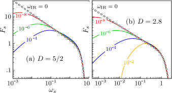
Figure S1: Self-similar profiles with (a) $D=5/2$, $J_{s}=0$, $S_{s}(\omega_{\mathrm{IR}})=-1$ and (b) $D=2.8$, $J_{s}(\omega_{s})=J_{0}\,\mathrm{sech}^{2}(\omega_{s}-\omega_{1})$, $J_{0}\approx 0.052$, and $\omega_{1}=1.2$. Numbers near the graphs give the values of $\omega_{\mathrm{IR}}$.

In Fig. S1(a) we show the solutions $F_{s}(\omega_{s})$ with ${D=5/2}$ and $S_{s}(\omega_{\mathrm{IR}})=-1$, while Fig. S1(b) visualizes the case $J_{s}\neq 0$ and ${D=2.8}$. It is clear that the self-similar profiles have definite limits $\omega_{\mathrm{IR}}\to 0$. Indeed, Eq. (S8) suggests an infrared asymptotic 

$$F_{s}=F_{0s}\,\omega_{s}^{-1/2}+F_{1s}\,\omega_{s}+O(\omega_{s}^{3/2})\dots\;\;\mbox{as}\;\;\omega_{s}\to 0$$ (S9)

in the unregularized case $\omega_{\mathrm{IR}}=0$, where $F_{0s}$, $F_{1s}$ are constants. Imposing this behavior, we obtain the ${\omega_{\mathrm{IR}}=0}$ graphs in Fig. S1 (chain points). Note that Eq. (S9) includes a thermal tail at $\omega_{s}\to 0$, which is indeed observed at $\omega_{\mathrm{IR}}\ll\omega_{s}\ll\omega_{1}$ in the full numerical simulations, see Fig. 1(c) from the main text.

The profile with $\omega_{\mathrm{IR}}=10^{-2}$ from Fig. S1(b) is repeated in Figs. 1(a) and (c) of the main text. It has $J_{s}(\omega_{s})=J_{0}\,\mathrm{sech}^{2}(\omega_{s}-\omega_{1})$, $J_{0}\approx 0.052$, and $\omega_{1}=1.2$. These parameters are selected to fit the simulation data.

Another good remark is that the self-similar profiles fall off as fast as ${F_{s}\propto\omega_{s}^{q}\,\mathrm{e}^{-\zeta\,\omega_{s}^{5/2}}}$ at ${\omega_{s}\to+\infty}$, where $q=(4-D)/(2D-4)$ and $\zeta=(2D-4)/\lim\limits_{\omega_{s}\to\infty}{(5DA\sqrt{\omega_{s}})}$. The cutoff appears because gravitational scattering is ineffective at high $\omega$. Above the cutoff, the particles cannot participate in self-similar dynamics.

To summarize, the profile equation (S8) has two families of nontrivial solutions: one solution per every $J_{s}$ at $D>5/2$ and a branch of $D=5/2$ solutions with arbitrary condensation flux $S_{s}(\omega_{\mathrm{IR}})$ and zero source.

D. Attracting to self-similar solutions

Figure S2: Evolutions of the ratio $E_{b}^{3}/M_{b}^{5}$ in all our Schrödinger-Poisson simulations (pale solid lines). These runs have essentially different $t_{gr}$, see Sec. 4 of the main text. Chain points show the law (7) with ${\tau_{i}=-0.1}$ and ${\tau_{*}=1.1\cdot(1-x_{e})^{5}}$.

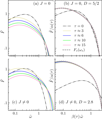
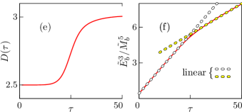
Figure S3: Numerical solutions of the modified kinetic equation (S10). Figure (a) is plotted for $\tilde{J}=0$, while (c) considers self-similar source $\tilde{J}=\alpha(\tau)J_{s}(\beta(\tau)\tilde{\omega})/(\tau-\tau_{i})$ with $J_{s}(\omega_{s})=J_{0}\,\mathrm{sech}^{2}(\omega_{s}-\omega_{1})$, $J_{0}\approx 0.1$, $\omega_{1}=1.2$, $D=2.8$, and $\tau_{i}=-0.1$. (b), (d) Transformations (3), (S11) of the spectra (a) and (c) with parameters (b) $D=5/2$, $\tau_{i}\approx-1.9$ and (d) $D=2.8$, ${\tau_{i}=-0.1}$ (lines). Chain points show self-similar profiles $F_{s}(\omega_{s})$ with regulators (b) $\omega_{\mathrm{IR}}=2\cdot 10^{-3}$ and (d) $\omega_{\mathrm{IR}}=4.5\cdot 10^{-4}$. (e), (f) Evolutions of ${D=D(\tau)}$ and $E_{b}^{3}/M_{b}^{5}$ in the case of essentially non self-similar source (lines).

Let us demonstrate that the self-similar solutions (3) are attractors of kinetic evolution.

To warm up, we explicitly test Eq. (7) using full Schrödinger-Poisson simulations. Recall that this law approximately describes self-similar bath with slowly-varying $D=D(\tau)$. We compute the bath masses $M_{b}(t)$ and energies $E_{b}(t)$ for all our solutions from Figs. 1 and 2 using the distribution functions $F(t,\,\omega)$ at ${\omega>0}$. This gives $M_{b}=M-M_{*}$ and $E_{b}=E-E_{*}$. Then in Fig. S2 we plot the left-hand side of Eq. (7) versus the right-hand side, i.e. basically $E_{b}^{3}/M_{b}^{5}$ as functions of $\tau$ (pale solid lines). The resulting curves are close to each other and are well described by Eq. (7) (chain points) despite essentially different parameters of the solutions. This confirms self-similar character of the bath evolution and, hence, our theory for Bose star growth.

Next, we consider time-dependent kinetic equation (4), (S3). To account for condensation onto the Bose star, we introduce an absorbing sink $\tilde{W}$ at $\tilde{\omega}\approx 0$ and an energy source $\tilde{J}$,

$$\partial_{\tau}\tilde{F}=-\partial_{\tilde{\omega}}\tilde{S}-\tilde{W}(\tilde{\omega})\tilde{F}+\tilde{J}(\tau,\,\tilde{\omega})\,.$$ (S10)

In practice, we use the sink profile $\tilde{W}=W_{0}\,\mathrm{e}^{-(\tilde{\omega}/\omega_{\mathrm{IR}}^{\prime})^{2}}$ concentrated at $\tilde{\omega}\lesssim\omega_{\mathrm{IR}}^{\prime}$. It effectively destroys low-energy particles at $W_{0}=200/\omega_{\mathrm{IR}}^{\prime}$ and $\omega_{\mathrm{IR}}^{\prime}=4\cdot\mathrm{10}^{-4}$. We start simulations from the Gaussian-distributed (virialized) initial state ${\tilde{F}(0,\,\tilde{\omega})\propto\tilde{\omega}^{1/2}\,\mathrm{e}^{-2\tilde{\omega}}}$ and play with different $\tilde{J}(\tau,\,\tilde{\omega})$.

Figure S3(a) shows the numerical solution $\tilde{F}(\tau,\,\tilde{\omega})$ at ${\tilde{J}=0}$. This is the case when the energy of the bath is (almost) conserved and the mass is not: recall that the sink swallows particles with $\tilde{\omega}\approx 0$. The self-similar profile with such properties has $D\approx 5/2$, see Eq. (6). In Fig. S3(b) (dash-dotted and solid lines) we perform self-similar rescaling of the spectra (a) with $D=5/2$ and

$$\alpha(\tau)=(\tau-\tau_{i})^{-1/D}\,,\;\;\;\;\;\;\beta(\tau)=(\tau-\tau_{i})^{2/D-1}\,,$$ (S11)

where the time-translation parameter $\tau_{i}$ is restored as compared to Eq. (3). We see that for properly adjusted $\tau_{i}\approx-1.9$ all of the rescaled graphs except for the one with $\tau=0$ merge into a single curve coinciding with $D=5/2$ self-similar profile $F_{s}(\omega_{s})$ (chain points). It is worth noting that the absorbing sink is implemented differently in our calculations of $F_{s}$ and $\tilde{F}$ — hence the difference in their infrared regulators $\omega_{\mathrm{IR}}$ and $\omega_{\mathrm{IR}}^{\prime}$. We see that although the starting distribution does not resemble the self-similar profile at all, the evolved spectra approach $\alpha F_{s}(\beta\tilde{\omega})$ at $\tau\sim 3$ and remain close to it at later times. This proves that the self-similar solution with $D=5/2$ is an attractor at $\tilde{J}=0$.

Now, add the energy source with self-similar time dependence: $\tilde{J}=\alpha(\tau)J_{s}(\beta(\tau)\tilde{\omega})/(\tau-\tau_{i})$, where $J_{s}(\omega_{s})$ has the same form as in Fig. 1; $D=2.8$ and $\tau_{i}=-0.1$. The respective solution $\tilde{F}(\tau,\,\tilde{\omega})$ of the kinetic equation is visualized in Fig. S3(c). At late times, it exhibits the self-similar behavior with $D=2.8$. Indeed, the rescaled spectra in Fig. S3(d) (lines) coincide at $\tau>3$ with the $D=2.8$ self-similar profile (chain points). Again, we see that the self-similar solutions are attractors.

Note that the scaling weight $D$ of the solution does not always correspond to the time dependence of the external source. If the amplitude of $\tilde{J}$ is too large or too small, the function $\tilde{F}(\tau,\,\tilde{\omega})$ first attracts to the self-similar profile with different $D$. Later, the weight starts to evolve slowly until the source-prescribed value is reached. In such a case, the dynamics remains approximately self-similar at all times but $D$ slowly drifts with $\tau$.

The latter situation is illustrated in Figs. S3(e), (f), where we consider the source $\tilde{J}=J_{0}\,\vartheta(\tau)\,\mathrm{sech}^{2}(\tilde{\omega}-\omega_{1})$ switching on at $\tau\sim 25$ as $\vartheta(\tau)=[1+\mathrm{e}^{(\tau_{i}^{\prime}-\tau)/\Delta\tau}]^{-1}(\tau-\tau_{i})^{-2/3}$, where $J_{0}\approx 0.017$, $\omega_{1}=1.2$, $\tau_{i}\approx-0.6$, $\tau_{i}^{\prime}\approx 24$, and $\Delta\tau\approx 2.3$. This time dependence of $\tilde{J}(\tau,\,\tilde{\omega})$ explicitly breaks the scaling symmetry of Eq. (S10) making the parameter $D=(3R-5)/(R-2)$ in Fig. S3(e) jump from $D\approx 5/2$ in the beginning of the process to almost $3$ in the end; to plot the figure, we extracted $R\equiv d\ln E_{b}/d\ln M_{b}$ from the numerical evolution. Nonetheless, the combination $E_{b}^{3}/M_{b}^{5}$ [solid line in Fig. S3(f)] becomes almost linear in the late-time region where $D=D(\tau)$ starts to evolve slowly, again — see the linear fits (chain points). This confirms that the solution attracts to self-similarity even after the strong kick at $\tau\approx 25$.

It is worth noting, however, that the tilts of the linear graphs in Fig. S3(f) are different at early and late times. This implies that Eq. (7) holds, but the parameter $\tau_{*}$ insubstantially changes with time. The latter change is ignored in the main text but should be taken into account in the refined approaches.

To summarize, we numerically proved that self-similar solutions (3) are attractors of kinetic evolution with a sink at $\tilde{\omega}\approx 0$ and an energy source.

E. Self-interacting bosons

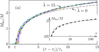
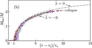
Figure S4: Mass evolution of Bose stars in the model with nonzero self-coupling at $\epsilon\approx 0.186$ and (a) $\tilde{\lambda}=15$, (b) ${\tilde{\lambda}=-6}$. Thin color lines display results of 9+8 simulations, whereas thick dashed is the theory with (a) ${\tau_{i}\approx-0.51}$, $x_{e}\approx 0.023$; (b) $\tau_{i}\approx 0.14$, $x_{e}\approx 0.026$. For reference, we repeat the theoretical curve with $\lambda=0$ and $\epsilon\approx 0.186$ from Fig. 2(b) (thin dash-dotted line). The inset of Fig. (a) shows the theoretical curves with $\tilde{\lambda}=0$ and $\tilde{\lambda}=15$ at larger timescales.

A highly nontrivial test  of our theoretical framework can be performed by studying growth of Bose stars in the bath of self–interacting bosons. We describe self-interactions by adding the term $\lambda|\psi^{2}|\psi/(8m^{2})$ with coupling constant $\lambda$ to the right–hand side of the upper Eq. (1). This upgrades the full set to Gross–Pitaevskii–Poisson system.

In the presence of gravity, a comparative effect of self-interactions is characterized by a dimensionless combination Dmitriev et al. (2021) $\tilde{\lambda}=2\lambda\omega_{0}/(m^{3}G)$, where $\omega_{0}$ is the typical particle energy. Our self-similar solution (7) is applicable if gravity dominates, i.e. at Levkov, Panin, and Tkachev (2018); Chen et al. (2022)

$$\frac{\tau_{gr}}{\tau_{\lambda}}\sim\ \frac{\sigma_{\lambda}}{\sigma_{gr}}\simeq\frac{\tilde{\lambda}^{2}}{1024\pi^{2}\ln(p_{0}L)}\ll 1\,.$$ (S12)

Here $\tau_{gr}$ and $\tau_{\lambda}$ are the gravitational and self-interaction relaxation times, while $\sigma_{gr}$ and $\sigma_{\lambda}$ are the respective transport cross sections. Below we keep  $\tau_{gr}/\tau_{\lambda}\lesssim 10^{-2}$ in all simulations.

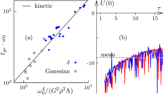
Figure S5: (a) The times $\omega_{0}t_{gr}$ of Bose stars formation in miniclusters versus the relevant factor in the theoretical expression for this quantity; $\Lambda\equiv\ln(p_{0}R)$ is the Coulomb logarithm and $R$ is the minicluster size. Filled and empty points correspond to simulations of Ref. Levkov, Panin, and Tkachev (2018) starting from the $\delta$–distributed gas and our solutions with Gaussian initial conditions, respectively. Thin solid line is the theory with $b=0.7$. (b) Time–dependent potential $U(0)$ in the minicluster center (dimensionless units). Thin solid graphs are extracted from two long simulations, while the dashed line is the time–averaged value.

Despite Eq. (S12), self–interactions can modify the growth law of Bose stars, and their effect can be considerable Chen et al. (2021). Indeed, although the terms proportional to $\lambda$ are small inside the light stars, they grow with mass and start to dominate Chavanis and Delfini (2011) at $M_{bs}\gtrsim M_{\lambda}\equiv|\lambda G|^{-1/2}$. If the self-interactions are repulsive, $\lambda>0$, this increases the energy of heavy stars to $E_{bs}\propto-M_{bs}^{2}$. The attractive case is more dramatic: negative self-pressure makes the Bose stars collapse Chavanis and Delfini (2011); Eby et al. (2016); Levkov, Panin, and Tkachev (2017); Chen et al. (2021) as Bosenovas at $M_{bs}\gtrsim 10.2\,M_{\lambda}$. Generically, we write

$$E_{bs}=-\gamma M_{bs}^{3}\,{\cal E}(M_{bs}/M_{\lambda})\,,$$ (S13)

where the function ${\cal E}$ accounts for self-interaction energy. It is smaller (larger) than $1$ at $\lambda>0$ ($\lambda<0$). Besides, ${\cal E}\approx 1$ at $M_{bs}\ll M_{\lambda}$ when the self-interactions are negligible. In practice, we compute ${\cal E}$ numerically by solving the Gross–Pitaevskii–Poisson system for every $M_{bs}/M_{\lambda}$.

Using Eq. (7), we obtain the growth law of self-interacting stars [cf. Eq. (8)],

$$(1+x_{bs}^{3}{\cal E}/\epsilon^{2})^{3}(1-x_{e}-x_{bs})^{-5}\approx(\tau-\tau_{i})/\tau_{*}\,,$$ (S14)

where ${\cal E}\equiv{\cal E}(x_{bs}M/M_{\lambda})$. At the qualitative level, Eq. (S14) agrees with the phenomenon suggested in Ref. Chen et al. (2021): for fixed $\tau_{*}$ and $\tau_{i}$ the Bose stars grow faster for positive $\lambda$ (${\cal E}<1$) and slower for negative $\lambda$ (${\cal E}<1$). This feature is illustrated in Figs. S4(a), (b) that compare two theoretical curves $x_{bs}(\tau)$, Eq. (S14), at $\tilde{\lambda}=15$ and $\tilde{\lambda}=-6$ (thick dashed lines) with the one at $\lambda=0$ (thin dash-dotted).

We performed an explicit numerical test of Eq. (S14). Starting from the Gaussian-distributed gas in the box, we performed 9 simulations at $\tilde{\lambda}=15$ and 8 simulations at $\tilde{\lambda}=-6$. We used $M=20\,p_{0}/m^{2}G$ and ${L=(35\div 40)/p_{0}}$. Mass evolutions of the respective Bose stars are shown in Figs. S4a, b by thin color lines. They are well described by Eq. (S14) (thick dashed). However, the values of the fitting parameter  $\tau_{i}$ are different with respect to non self–interacting case: we obtain $\tau_{i}\approx-0.51$ at $\tilde{\lambda}=15$ and  $\tau_{i}\approx 0.14$ at $\tilde{\lambda}=-6$.

It is worth noting that the dependence of $\tau_{i}$ on $\tilde{\lambda}$ affects the growth law of Bose stars. At moderately small $\tau$, it may even compensate the (de)acceleration effect of self–interaction energy, see the inset in Fig. S4(a). However, at large timescales the self–energy wins and makes the growth go faster at $\lambda>0$ and slower at $\lambda<0$ — see the inset, again.

F. Simulations in miniclusters

Although the application of our theory (8) is straightforward at the qualitative level, things become more tricky once precise agreement with simulations is required. To this end, we accurately determine the minicluster parameters.

We form gravitationally bound miniclusters by triggering strong Jeans instability in the dense virialized gas Levkov, Panin, and Tkachev (2018); Chen et al. (2021). In particular, our two long simulations start from very large mass $M_{\mathrm{tot}}=112.5/\omega_{0}$ in the box $L=52.5/p_{0}$. At these values, the miniclusters engulf more than $55\%$ of matter, and the remaining diffuse particles do not affect much the growth of objects within them.

We define the minicluster center as the center-of-mass of matter distribution within the box; we call it $\boldsymbol{x}=0$ for simplicity. The density $\bar{\rho}=\rho(0)$ in the minicluster center is then obtained as the value of $\rho=m|\psi(t,\,\boldsymbol{x})|^{2}$ averaged over the Gaussian spatial window. The remaining parameters are extracted from the distribution function (2) or, specifically, from its part at $\omega<0$ that describes a self-bound minicluster. Namely, the mass $M$ and energy $E_{\mathrm{mc}}<0$ of the minicluster are obtained by integrating $F$ and $\omega F/m$ over this region. Then the virial particle energy equals $\omega_{0}\equiv-mE_{\mathrm{mc}}/M$, the virial radius is $R=(3\omega_{0}/2\pi mG\bar{\rho})^{1/2}$, while $\Lambda=\ln(p_{0}R)$ is the Coulomb logarithm.

Once the minicluster parameters are specified, we find the numerical factor  $b$ in the expression for the relaxation time $t_{gr}$. To this end we perform many short-time simulations at different values of parameters and wait until Bose stars appear in their miniclusters. The moments $t_{gr}$ when they form (empty points in Fig. S5(a)) are well described by the theory with $b=0.7$ (line) — the same value as in Ref. Levkov, Panin, and Tkachev (2018). The coincidence of $b$’s is remarkable because minicluster simulations of Ref. Levkov, Panin, and Tkachev (2018) (filled points) start from the $\delta$-distributed gas in the box, $|\psi_{\boldsymbol{p}}|^{2}\propto\delta(|\boldsymbol{p}|-p_{0})$, while our simulations use Gaussian gas with $|\psi_{\boldsymbol{p}}|^{2}\propto\mathrm{e}^{-\boldsymbol{p}^{2}/p_{0}^{2}}$. This suggests that formation of miniclusters strongly intermixes the gas forcing it to “forget” the initial condition.

An important part of our procedure is a computation of the gravitational potential $U(0)$ in the minicluster center. In the notations of Eqs. (7), (8), this parameter enters the total energy $E=E_{\mathrm{mc}}-U(0)M$ which is positive and counted from the lowest level inside the minicluster. Notably, the value of $U(0)$ visibly drifts with time, since the minicluster gets eaten by the Bose star and becomes lighter; see Fig. S5(b). We calculate the potential using the Bose star itself as a sensor. On the one hand, its mass $M_{bs}$ and binding energy $\omega_{bs}=-3m\gamma M_{bs}^{2}$ can be extracted from the profile $|\psi_{bs}(\boldsymbol{x})|^{2}$. On the other, the “Bose star” peak in the energy distribution is located at $\omega=\omega_{bs}+mU(0)$. Subtracting these quantities, we obtain the solid lines in Fig. S5(b) corresponding to two long simulations. We use the time-averaged value of $U(0)$ (dashed horizontal line) in the theoretical expressions for $E$ and $\epsilon^{2}=E/\gamma M^{3}$.

Finally, we determine the fraction $x_{e}=M_{e}/M$ of particles on the discrete levels of the Bose star potential in the same way as before: by integrating $F$ over the region $\omega_{bs}+mU(0)<\omega<mU(0)$. Once this is done, the theoretical predictions (S14) match the Bose star mass curves extracted from the simulations (lower graph in Fig. 2(b)). The respective best-fit value $\tau_{i}\approx-0.1$ matches that in the box simulations.

References

- Ruffini and Bonazzola (1969) R. Ruffini and S. Bonazzola, Phys. Rev. 187, 1767 (1969).
- Tkachev (1986) I. I. Tkachev, Sov. Astron. Lett. 12, 305 (1986).
- Ringwald, Rosenberg, and Rybka (2022) A. Ringwald, L. J. Rosenberg, and G. Rybka, in Review of Particle Physics, PTEP 2022, 083C01 (2022).
- Niemeyer (2020) J. C. Niemeyer, Prog. Part. Nucl. Phys. 113, 103787 (2020), arXiv:1912.07064 .
- Schive, Chiueh, and Broadhurst (2014) H.-Y. Schive, T. Chiueh, and T. Broadhurst, Nature Phys. 10, 496 (2014), arXiv:1406.6586 .
- Tkachev (1991) I. I. Tkachev, Phys. Lett. B261, 289 (1991).
- Levkov, Panin, and Tkachev (2018) D. G. Levkov, A. G. Panin, and I. I. Tkachev, Phys. Rev. Lett. 121, 151301 (2018), arXiv:1804.05857 .
- Eggemeier and Niemeyer (2019) B. Eggemeier and J. C. Niemeyer, Phys. Rev. D 100, 063528 (2019), arXiv:1906.01348 .
- Chen et al. (2021) J. Chen et al., Phys. Rev. D 104, 083022 (2021), arXiv:2011.01333 .
- (10) J. H.-H. Chan, S. Sibiryakov, and W. Xue, arXiv:2207.04057 .
- Note (1) Self-similar solutions are well-known in kinetic theory with short-range interactions Semikoz and Tkachev (1995); *Micha:2002ey; *Micha:2004bv; *SEMISALOV2021105903 and in dynamical long-range problems like collapse Choptuik (1993); *Maeda:2004kw; *Gundlach:2007gc or infall Bertschinger (1985); *Sikivie:1996nn. But their relevance for kinetics caused by gravitational (long-range) scattering was not observed before.
- Kolb and Tkachev (1993) E. W. Kolb and I. I. Tkachev, Phys. Rev. Lett. 71, 3051 (1993), arXiv:hep-ph/9303313 .
- Kolb and Tkachev (1994a) E. W. Kolb and I. I. Tkachev, Phys. Rev. D49, 5040 (1994a), arXiv:astro-ph/9311037 .
- Vaquero, Redondo, and Stadler (2019) A. Vaquero, J. Redondo, and J. Stadler, JCAP 04, 012 (2019), arXiv:1809.09241 .
- Buschmann, Foster, and Safdi (2020) M. Buschmann, J. W. Foster, and B. R. Safdi, Phys. Rev. Lett. 124, 161103 (2020), arXiv:1906.00967 .
- Eggemeier et al. (2020) B. Eggemeier et al., Phys. Rev. Lett. 125, 041301 (2020), arXiv:1911.09417 .
- Ellis, Marsh, and Behrens (2021) D. Ellis, D. J. E. Marsh, and C. Behrens, Phys. Rev. D 103, 083525 (2021), arXiv:2006.08637 .
- Note (2) Equations (1\@@italiccorr) have exact scaling symmetry changing ; see, e.g., Schive, Chiueh, and Broadhurst (2014); Levkov, Panin, and Tkachev (2018). This makes the solution depend on dimensionless combinations , , and .
- Simulation movie for and ; cf. Figs. 1, 2. Four panels show time evolutions of —ψ(x)—^2M_bs(2023) (~ω) Simulation movie for and ; cf. Figs. 1, 2. Four panels show time evolutions of , the rescaled distribution (3), particle density , and (top to bottom, left to right), https://www.youtube.com/playlist?list=PLMxQF3HFStX0_CFowbYStkjRv-xZEG-Vn (2023).
- Lifshitz and Pitaevskii (2012) E. Lifshitz and L. Pitaevskii, Course of Theoretical Physics, Vol. 10: Physical Kinetics (Elsevier Science, 2012).
- Zakharov and Karas’ (2013) V. E. Zakharov and V. I. Karas’, Physics Uspekhi 56, 49 (2013).
- Skipp, L’vov, and Nazarenko (2020) J. Skipp, V. L’vov, and S. Nazarenko, Phys. Rev. A 102, 043318 (2020), arXiv:2003.05558 .
- Zakharov, L’vov, and Falkovich (2012) V. Zakharov, V. L’vov, and G. Falkovich, Kolmogorov Spectra of Turbulence I: Wave Turbulence (Springer, 2012).
- Note (3) Our best-fit value from Figs. 2 and SM-S2 is quite small and does not affect the agreement in Fig. 1(c).
- Lee and Pang (1989) T. D. Lee and Y. Pang, Nucl. Phys. B 315, 477 (1989).
- Dmitriev et al. (2021) A. S. Dmitriev et al., Phys. Rev. D 104, 023504 (2021), arXiv:2104.00962 .
- Note (4) More precise expression follows from the adiabatic theorem: , where depends on the occupation numbers of the bound states.
- Schwabe, Niemeyer, and Engels (2016) B. Schwabe, J. C. Niemeyer, and J. F. Engels, Phys. Rev. D 94, 043513 (2016), arXiv:1606.05151 .
- Mocz et al. (2017) P. Mocz et al., MNRAS 471, 4559 (2017), arXiv:1705.05845 .
- Schive et al. (2014) H.-Y. Schive et al., Phys. Rev. Lett. 113, 261302 (2014), arXiv:1407.7762 .
- Bar et al. (2018) N. Bar et al., Phys. Rev. D 98, 083027 (2018), arXiv:1805.00122 .
- Mina, Mota, and Winther (2022) M. Mina, D. F. Mota, and H. A. Winther, Astron. Astrophys. 662, A29 (2022), arXiv:2007.04119 .
- (33) J. L. Zagorac et al., arXiv:2212.09349 .
- Chan et al. (2022) H. Y. J. Chan et al., MNRAS 511, 943 (2022), arXiv:2110.11882 .
- Nori and Baldi (2021) M. Nori and M. Baldi, Mon. Not. Roy. Astron. Soc. 501, 1539 (2021), arXiv:2007.01316 .
- Schwabe and Niemeyer (2022) B. Schwabe and J. C. Niemeyer, Phys. Rev. Lett. 128, 181301 (2022), arXiv:2110.09145 [astro-ph.CO] .
- (37) Z. Li et al., ApJ 889, 88, arXiv:2001.00318 .
- Eggemeier et al. (2022) B. Eggemeier et al., Phys. Rev. D 105, 023516 (2022), arXiv:2110.15109 .
- Ellis et al. (2022) D. Ellis et al., Phys. Rev. D 106, 103514 (2022), arXiv:2204.13187 .
- (40) X. Du et al., arXiv:2301.09769 .
- Kolb and Tkachev (1994b) E. W. Kolb and I. I. Tkachev, Phys. Rev. D 50, 769 (1994b), arXiv:astro-ph/9403011 .
- Klaer and Moore (2017) V. B. Klaer and G. D. Moore, JCAP 1711, 049 (2017), arXiv:1708.07521 .
- Gorghetto, Hardy, and Villadoro (2018) M. Gorghetto, E. Hardy, and G. Villadoro, JHEP 07, 151 (2018), arXiv:1806.04677 .
- Gorghetto, Hardy, and Villadoro (2021) M. Gorghetto, E. Hardy, and G. Villadoro, SciPost Phys. 10, 050 (2021), arXiv:2007.04990 .
- Levkov, Panin, and Tkachev (2020) D. G. Levkov, A. G. Panin, and I. I. Tkachev, Phys. Rev. D 102, 023501 (2020), arXiv:2004.05179 .
- Eby et al. (2022) J. Eby et al., Phys. Lett. B 825, 136858 (2022), arXiv:2106.14893 .
- Visinelli (2021) L. Visinelli, Int. J. Mod. Phys. D 30, 2130006 (2021), arXiv:2109.05481 .
- (48) M. Escudero et al., arXiv:2302.10206 .
- Rogers and Peiris (2021) K. K. Rogers and H. V. Peiris, Phys. Rev. Lett. 126, 071302 (2021), arXiv:2007.12705 .
- Note (5) This solution satisfies as .
- Note (6) We thank the Referee for suggesting this check.
- Chen et al. (2022) J. Chen, X. Du, E. W. Lentz, and D. J. E. Marsh, Phys. Rev. D 106, 023009 (2022), arXiv:2109.11474 .
- Note (7) This ratio is even smaller in magistral cosmological models. For example, and Levkov, Panin, and Tkachev (2018); Chen et al. (2022) inside QCD axion miniclusters. At these values, the effect of self-interactions on growth of Bose stars is negligible. To make them relevant, one switches Chen et al. (2021, 2022) to general “axion–like” models with deliberately enlarged .
- Chavanis and Delfini (2011) P. H. Chavanis and L. Delfini, Phys. Rev. D 84, 043532 (2011), arXiv:1103.2054 .
- Eby et al. (2016) J. Eby et al., JHEP 12, 066 (2016), arXiv:1608.06911 .
- Levkov, Panin, and Tkachev (2017) D. G. Levkov, A. G. Panin, and I. I. Tkachev, Phys. Rev. Lett. 118, 011301 (2017), arXiv:1609.03611 .
- Note (8) We still extract from the distribution function and compute using the initial data. The value of is fixed by the condition at , see Sec. 4.
- Note (9) This is a necessary part of the procedure compensating for our voluntary choice of the minicluster parameters , , and .
- Semikoz and Tkachev (1995) D. V. Semikoz and I. I. Tkachev, Phys. Rev. Lett. 74, 3093 (1995), arXiv:hep-ph/9409202 .
- Micha and Tkachev (2003) R. Micha and I. I. Tkachev, Phys. Rev. Lett. 90, 121301 (2003), arXiv:hep-ph/0210202 .
- Micha and Tkachev (2004) R. Micha and I. I. Tkachev, Phys. Rev. D 70, 043538 (2004), arXiv:hep-ph/0403101 .
- Semisalov et al. (2021) B. Semisalov et al., Communications in Nonlinear Science and Numerical Simulation 102, 105903 (2021), arXiv:2104.14591 .
- Choptuik (1993) M. W. Choptuik, Phys. Rev. Lett. 70, 9 (1993).
- Maeda and Harada (2005) H. Maeda and T. Harada, “Kinematic self-similar solutions in general relativity,” in General Relativity Research Trends. Horizons in World Physics, Vol. 249 (Nova Science Publishers, New York, 2005) p. 123, arXiv:gr-qc/0405113 .
- Gundlach and Martin-Garcia (2007) C. Gundlach and J. M. Martin-Garcia, Living Rev. Rel. 10, 5 (2007), arXiv:0711.4620 .
- Bertschinger (1985) E. Bertschinger, Astrophys. J. Suppl. 58, 39 (1985).
- Sikivie, Tkachev, and Wang (1997) P. Sikivie, I. I. Tkachev, and Y. Wang, Phys. Rev. D 56, 1863 (1997), arXiv:astro-ph/9609022 .