Adaptive Estimation-Based Safety-Critical Cruise Control of Vehicular Platoons

Abstract

Optimal cruise control design can increase highway throughput and vehicle safety in traffic flow. In most heterogeneous platoons, the absence of vehicle-to-vehicle (V2V) communication poses challenges in maintaining system stability and ensuring a safe inter-vehicle distance. This paper presents an adaptive estimation-based control design for adaptive cruise control (ACC) that swiftly estimates the states of the preceding vehicle while operating the autonomous vehicle within a safe region. Control Lyapunov Functions (CLFs) and Control Barrier Functions (CBFs) are employed to design a safety-critical controller that ensures safety despite potential estimation errors. The proposed estimator-controller framework is implemented in scenarios with and without vehicle-to-vehicle communication, demonstrating successful performance in maintaining platoon safety and stability. Additionally, physics engine-based simulations reinforce both the practical viability of the proposed control framework in real-world situations and the controller’s adeptness at ensuring safety amidst realistic environmental conditions.

I Introduction

The rapid evolution of autonomous vehicles is revolutionizing the way we commute. One crucial aspect of autonomous vehicle design is the development of effective and safe controllers. A variety of control scenarios must be addressed in the design process, including lane changes, intersections, parking, and cruise control. Among these, cruise control has attracted considerable research interest due to its wide-ranging applications in vehicle platooning, eco-driving on signalized corridors, and traffic management [1]. Two prominent types of cruise control implementation are Adaptive Cruise Control (ACC) and Connected Cruise Control (CCC). Designing safety-critical controllers for ACC and CCC presents significant challenges, such as handling noisy sensors and input delays while ensuring system stability [2]. In the case of CCC, vehicles can communicate their states, necessitating that the controller account for communication delays. In contrast, ACC systems lack communication capabilities, which poses the challenge of designing controllers independent of the actual states of the preceding vehicle. Most research uses a state estimator to tackle this challenge.

Over the years, numerous controllers have been developed to address these challenges. Some research has focused on handling communication delays, noise, and input delays. Controller design in the presence of input delay and disturbances is discussed in [3]. A cooperative adaptive controller design for noisy and delay-inducing communication channels is presented in [4]. State prediction for designing optimal control law for CCC systems using LQR optimization is explored in [5]. Meanwhile, other research has concentrated on observer and controller designs for ACC. An acceleration estimator design for a cruise control system when only distance and velocity information is communicated, employing a state feedback controller to maintain a safe distance, is proposed in [6]. An acceleration observer control design in the discrete-time frame is introduced in [7]. The authors in [8] have presented a prediction model to determine velocity distribution and used it with other safety constraints in a model predictive controller for energy-efficient cruise control. Some literature has also focused on optimization and learning-based control design for cruise control. A comparison of Deep Reinforcement Learning (DRL) and Model Predictive Control (MPC) for ACC is discussed in [9]. A PID controller using genetic algorithm optimization for cruise control is presented in [10]. A T-NMPC method is used in [11] to handle the vehicle constraints robustly while adapting to system changes and improving the performance of Economic Autonomous Cruise Control (Eco-ACC) systems. Additionally, the authors in [12] designed a DRL-based CCC controller and demonstrated its application to various traffic system conditions with different communication delays, initial states, reward function forms, and the number of vehicles.

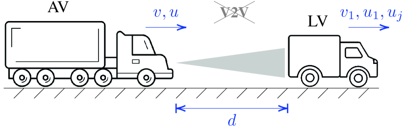
Figure 1: Predecessor-successor configuration in Adaptive Cruise Control.

In cruise control applications, controllers must prioritize safety. The recent introduction of control barrier functions (CBF) offers an approach for the safety analysis of controllers [13]. The authors in [14] have presented a technique to integrate observer design and estimation error with CBF for safety-critical systems. CBF is employed in [15] to achieve safe, dynamic behavior in CCC applications, and a robust safety controller is designed to estimate the effect of disturbances on safety. A method for achieving string stability with bounded speed and acceleration while ensuring safe operation is presented in [16]. The safety enhancement techniques for CCC using CBFs are discussed in [17]. Although safety-critical control for CCC is well-researched, observer-based safety-critical controller design for ACC remains unexplored. To that end, the contributions of this paper are as follows: 1) an estimator design for the ACC systems to estimate both velocity and acceleration of the preceding vehicle in the absence of communication between vehicles; 2) a safety-critical controller design for ACC applications developed based on the estimator, which incorporates a thorough safety analysis and convergence proof using Control Lyapunov Functions (CLFs) and Control Barrier Functions (CBFs); 3) an adaptation law for the error bounds and conservative distance of the controller design to enhance the overall system performance; and 4) validation of the proposed controller by comparing the MATLAB generated results with the physics realistic AirSim environment [18] experimental results.

The paper is organized as follows: Section 2 discusses the ACC problem and system dynamics. Section 3 presents the estimator design, safety-critical controller design, stability analysis, and adaptive controller design. Section 4 analyzes and comments on the results. Finally, Section 5 concludes the paper and outlines potential avenues for future work.

II Problem Description

This section presents a formal description of the system dynamics and the Adaptive Cruise Control (ACC) problem. The cruise control problem is characterized by a platoon of $n$ autonomous vehicles and a leading vehicle. The primary objective is to follow the preceding vehicle while maintaining a safe distance and platoon stability. ACC emerges as a specialized subproblem within the broader cruise control domain, where each vehicle can only perceive its velocity and the distance between itself and the vehicle ahead, with no vehicle-to-vehicle communication.

II-A Platoon Dynamics

The dynamics of $(i-1)^{th}$ and $i^{th}$ vehicles in the platoon can be described using the predecessor-follower setup. This section discusses the predecessor-follower dynamics, while the extension to a complete platoon is addressed in the Results section. Let $d$ represent the distance between the two vehicles, $v_{1}$, $u_{1}$, and $u_{j}$ denote the velocity, acceleration, and jerk of the predecessor vehicle (LV), and $v$, $u$ represent the velocity and acceleration of the follower vehicle (AV) (see Fig. 1). The system dynamics can then be expressed as:

$$\dot{d} =v_{1}-v,\;\dot{v}_{1}=u_{1},\;\dot{v}=u,\;\dot{u}_{1}=u_{j}$$ (1)

To achieve maximum throughput in an ACC system, vehicles should follow their predecessors while maintaining the minimum possible distance and ensuring system stability. The distance satisfying both of these conditions [19] is given by equation (2), where $d_{r}>0$ represents the standstill distance and $T>0$ denotes the time headway.

$$d=d_{r}+Tv$$ (2)

Thus, any controller capable of maintaining $d\geq d_{r}+Tv$ is acceptable.

String stability [2] refers to the ability of a platoon of vehicles to maintain safe inter-vehicle distances and velocities under various driving conditions without amplifying disturbances as it propagates through the system. The quantification of string stability is accomplished through the use of the string stability gain, denoted as $\mathcal{S}$. This measure indicates the ratio of the disturbance amplitude of the preceding vehicle to the disturbance amplitude of the autonomous vehicle. A platoon is considered string stable if the disturbance amplitude decreases as it traverses the platoon. Consequently, platoons that have string stability gain $\mathcal{S}<1$ demonstrate string stability. According to this definition, a platoon system is deemed stable if it exhibits string stability and the inter-vehicular distance between each predecessor-follower pair adheres to a pre-established minimum safe distance $d_{r}+Tv$, and a finite upper bound.

III Estimator-based Safety Critical Controller

Adaptive Cruise Control (ACC) assumes no vehicle-to-vehicle (V2V) communication. Therefore, estimates of the predecessor vehicle’s velocity and acceleration are required to design an optimal controller. This section discusses the estimator design, safety-critical controller design, stability analysis, and adaptive controller design.

III-A Estimator Design

Let $\hat{d},\hat{v}$ and $\hat{u}$ represent the estimate of the state $d,v$, and $u$ respectively, and $\tilde{d},\tilde{v}$, and $\tilde{u}$ represent the error in the estimate, i.e., $\tilde{d}=\hat{d}-d$,$\tilde{v}=\hat{v}-v$, and $\tilde{u}=\hat{u}-u$, and $g_{1},g_{2},g_{3}$ be the constant estimator gains. Using this notation and the distance between the vehicles $d$ sensed by the AV, the state estimator dynamics is proposed as follows.

$$\dot{\hat{d}} =\hat{v}_{1}-v+g_{1}\tilde{d}$$ (3)

$$\dot{\hat{v}}_{1} =g_{2}\tilde{d}+\hat{u}_{1}$$

$$\dot{\hat{u}}_{1} =g_{3}\tilde{d}$$

Utilizing the estimator dynamics (3) and system dynamics (1), for estimation error $\tilde{e}=[\tilde{d},\,\tilde{v}_{1},\,\tilde{u}_{1}]^{T}$, the error dynamics can be formulated as:

$$\dot{\tilde{e}}=\begin{bmatrix}g_{1}&1&0\\ g_{2}&0&1\\ g_{3}&0&0\end{bmatrix}\tilde{e}+\begin{bmatrix}0\\ 0\\ -1\end{bmatrix}u_{j}=A\tilde{e}+Bu_{j}$$ (4)

Upper bounds on the error estimates of velocity and acceleration are introduced as $E_{v}\geq\tilde{v}_{1}$ and $E_{u}\geq\tilde{u}_{1}$, where $E_{v},E_{u}>0$. It is important to note that $E_{v}$ and $E_{u}$ represent upper bounds rather than absolute bounds. The choice of $E_{v}$ and $E_{u}$ affects the stability and equilibrium state of the system. The relation between these upper bounds and vehicle constraints is calculated in Section III-C, which can be used to choose the suitable values.

Assumption 1. To maintain the error estimates within bounds, the estimated error should be close to zero at $t=0$. To achieve this, $\tilde{v}$ and $\tilde{u}$ are assumed to be zero at $t=0$. This can be achieved by initiating communication with the predecessor vehicle (in the case of CCC) or starting from rest, i.e., $v_{1}=u_{1}=0$. This is a reasonable assumption for the ACC applications due to the fact that platoons generally originate from a designated location or commence their operation from a state of rest within a traffic environment.

III-B Safety-Critical Controller Design

The optimal controller design for the ACC problem is a safety-critical controller that ensures string stability while minimizing conservatism. The authors in [19] have presented that any controller capable of maintaining the inter-vehicle distance greater than or equal to $d_{r}+Tv$ (2), with a reasonable choice of time headway $T$, ensures string stability. To design such a controller, the concept of control barrier functions [13] is utilized.

For the given system, the function $h(d,v)=d-d_{r}-Tv$ characterizes the conservative behavior of the controller. The convergence and steady-state behavior of function $h$ can indicate the effectiveness of the control law. For an ideal controller, $h(d,v)=0,\forall t\geq 0$. Using this function, the safe set $\mathcal{C}\subset\mathbb{R}^{2}$ is defined as

$$\mathcal{C}=\{(d,v)\in\mathbb{R}^{2}:h(d,v)\geq 0\}$$ (5)

Definition 1: Given a safety set $\mathcal{C}\in\mathbb{R}^{2}$ defined by (5), the continuously differentiable function $h:\mathbb{R}^{2}\xrightarrow{}\mathbb{R}$ is considered a safety function if there exists an extended class $\mathcal{K}$ function [20] $\alpha$ such that

$$\dot{h}=v_{1}-v-Tu\geq-\alpha(h)\\$$ (6)

Hence, any $u$ satisfying equation (7) ensures safety:

$$\hat{v}_{1}-\tilde{v}_{1}-v+\alpha(h)\geq Tu$$ (7)

With $\kappa=\frac{1}{T}$ and $E_{v}\geq\tilde{v}_{1}$, the proposed controller design is:

$$u=\kappa\hat{v}_{1}-\kappa E_{v}-\kappa v+\kappa\alpha(h)$$ (8)

The controller proposed in (8) is designed following the platoon stability conditions, ensuring inherent stability. The stability response of the controller will be further analyzed with various scenarios in Section III-C to establish the conditions on $E_{v}$ and $\alpha(h)$ that guarantee stability.

Before proceeding to the stability analysis of the system, the estimator dynamics for the safety function $h(d,v)$ are derived as:

$$\hat{h} =h(\hat{d},v)=\hat{d}-d_{r}-Tv=\tilde{d}+h(\hat{d},v)$$ (9)

$$\dot{\hat{h}} =\hat{v}_{1}-v+g_{1}\tilde{d}-Tu$$

$$=E_{v}+g_{1}\tilde{d}-\alpha(\hat{h}-\tilde{d})$$ (10)

III-C Stability Analysis

Considering the error dynamics described by (4) and the estimate of safety function from (9, 10), the Lyapunov function candidates are investigated for the stability analysis of the ACC system in the two possible cases. Case 1 analysis proves that the controller design guarantees stability for constant preceding vehicle acceleration. Case 2 utilized case 1 to present that the controller behaves similarly in the presence of a non-zero jerk with a shifted equilibrium point. The stability analysis for case 1 is outlined as follows:

Case 1: $u_{j}=0$ (Constant preceding vehicle acceleration)

Consider the Lyapunov function candidate:

$$V_{1}(\tilde{e},\hat{d},v)=\frac{1}{2}(\hat{h}-d_{c})^{2}+\tilde{e}^{T}P\tilde{e}$$ (11)

where $d_{c}$ is the conservative distance constant and $P=P^{T}>0$ is the solution of the continuous algebraic Riccati equation [21]: $A^{T}P+PA+Q=0$, for $A$ given by (4) and $Q=Q^{T}>0$.

Lemma 1: For a given Hurwitz matrix $A$ and a positive definite matrix $Q$, there exists a unique positive definite matrix $P$ such that $A^{T}P+PA+Q=0$.

Lemma 1 implies that $V_{1}$ is a valid Lyapunov function candidate if the state matrix $A$ is Hurwitz. This sets a bound on the estimator design with the estimator gains $g_{1},g_{2},g_{3}<0$ (discussed in Appendix (V-A)).

Theorem 1: Given the Lyapunov function in (11), the control law in (8) and the safety function estimate dynamics in (10), the error estimate $\tilde{e}$ in (4) converges to zero and the conservative distance $h$ converges to $d_{c}$, for the specific choice of class $\mathcal{K}$ function $\alpha$, and distance constant $d_{c}$.

Proof: Computing the time derivative of $V_{1}$, the following is obtained:

$$\dot{V}_{1}(\tilde{e},\hat{d},v) =(\hat{h}-d_{c})\dot{\hat{h}}+\dot{\tilde{e}}^{T}P\tilde{e}+\tilde{e}^{T}P\dot{\tilde{e}}$$

$$=(\hat{h}-d_{c})\dot{\hat{h}}+\tilde{e}^{T}(A^{T}P+PA)\tilde{e}$$

$$=(\hat{h}-d_{c})(E_{v}+g_{1}\tilde{d}-\alpha(\hat{h}-\tilde{d}))-\tilde{e}^{T}Q\tilde{e}$$

By choosing the class $\mathcal{K}$ function as $\alpha(x)=-g_{1}x$, we have:

$$\dot{V}_{1}=(\hat{h}-d_{c})(E_{v}+g_{1}d_{c})-(\hat{h}-d_{c})\alpha(\hat{h}-d_{c})-\tilde{e}^{T}Q\tilde{e}$$ (12)

From (12), $\dot{V}_{1}$ becomes negative definite by selecting $d_{c}$ as:

$$d_{c}=-\frac{E_{v}}{g_{1}}\\$$ (13)

Then we obtain:

$$\dot{V}_{1}=-(\hat{h}-d_{c})\alpha(\hat{h}-d_{c})-\tilde{e}^{T}Q\tilde{e}<0$$ (14)

Since $\dot{V}_{1}$ is negative definite, it proves that the estimated error $\tilde{e}$ and conservative distance $h$ asymptotically converge to zero and $d_{c}$, respectively, where the steady state value of $h$ is defined as the conservative bias of the system.

Case 2: $u_{j}\neq 0$ (non zero preceding vehicle jerk)

For this case, as the preceding vehicle jerk is non-zero, the equilibrium point for the estimation error deviates from the origin. The shifted equilibrium point is obtained by setting $\dot{\tilde{e}}=0$ in (4), resulting in:

$$\tilde{e}^{*} =\begin{bmatrix}1\\ -g_{1}\\ -g_{2}\end{bmatrix}\frac{u_{j}}{g_{3}}$$ (15)

It is important to note that $u_{j}$ is used only to present the convergence guarantee of the safety-critical controller and estimator design. Similar to $d_{c}$, $u_{j}$ is not part of either the controller or the estimator dynamics. The derivation below shows that the system remains stable for any non-zero value of $u_{j}$. Therefore, the ACC system operating under the designed controller remains stable without any information on the actual value of the preceding vehicle’s jerk $u_{j}$. Consider the Lyapunov function candidate:

$$V_{2}(\tilde{e},\hat{d},v)=\frac{1}{2}(\hat{h}-d_{c})^{2}+\xi^{T}P\xi$$ (16)

with the positive-definite matrix $P$ in (11) and $\xi=\tilde{e}-\tilde{e}^{*}$. By following the same calculations as Theorem 1 for $V_{2}$, the following is obtained:

$$\dot{V}_{2}(\tilde{e},\hat{d},v) =(\hat{h}-d_{c})\dot{\hat{h}}+\dot{\xi}^{T}P\xi+\xi^{T}P\dot{\xi}$$

$$=(\hat{h}-d_{c})\dot{\hat{h}}+\xi^{T}(A^{T}P+PA)\xi$$

$$=(\hat{h}-d_{c})(E_{v}+g_{1}\tilde{d}-\alpha(\hat{h}-\tilde{d}))-\xi^{T}Q\xi$$

By choosing the same $\alpha(x)$ and $d_{c}$ as case 1, we obtain:

$$\dot{V}_{2}=-(\hat{h}-d_{c})\alpha(\hat{h}-d_{c})-\xi^{T}Q\xi<0$$ (17)

Since $\dot{V}_{2}$ is negative definite, it proves that $\xi$ converges to zero and $\hat{h}$ converges to $d_{c}$. Substituting these results into (9), the equilibrium value for $h$ is obtained as:

$$h^{*}=\hat{h}^{*}-\tilde{d}^{*}=\frac{-E_{v}}{g_{1}}-\frac{u_{j}}{g_{3}}$$ (18)

Substituting the safety bounds $h^{*}\geq 0$, $E_{v}\geq\tilde{v}$, and $E_{u}\geq\tilde{u}$, into (18) and $\xi\xrightarrow{}0$ gives:

$$E_{v}\geq-\frac{g_{1}u_{j}}{g_{3}}\;,\;E_{u}\geq-\frac{g_{2}u_{j}}{g_{3}}$$ (19)

Based on these bounds, a relationship between minimum $u_{j}$ $(U_{min})$, $E_{v}$, and $E_{u}$ is established:

$$E_{v}\geq-\frac{g_{1}U_{min}}{g_{3}}\;,\;E_{u}\geq-\frac{g_{2}U_{min}}{g_{3}}$$ (20)

Although, for ACC applications, $u_{j}$ is not known, $U_{min}$ is the lower bound on the jerk, which, in most cases, is a known vehicle property. If $U_{min}$ is unknown, any value guaranteed to be the lower bound can be used. The higher the difference between chosen value and the actual value, the higher the conservative behavior from the controller. Once $U_{min}$ is chosen, (20) can be used to choose the suitable upper bounds on velocity and acceleration error estimates. Remark: To maintain safety, it is necessary for $E_{v}\geq\tilde{v}_{1}$ $\forall\,t>0$. This can be achieved by selecting negative real eigenvalues for the state matrix A. Such eigenvalues guarantee a non-oscillatory convergence to the equilibrium point.

III-D Adaptive Error Dynamics

In previous sections, we established that an optimal control law strives to maintain the least conservative distance from the preceding vehicle. Although, according to (18) the conservative bias $h^{*}$ is proportional to the constant velocity error bound $E_{v}$ and the estimator gain $g_{1}$, the system’s transient behavior can be further optimized by incorporating adaptive dynamics for the error bound $E_{v}$. To make the controller adaptive and reduce the conservative bias, we introduce an adaptive state $\epsilon$ (as the velocity error bound) such that $E_{v}\geq\epsilon\geq\tilde{v}_{1}$. To enforce these bounds, a new control barrier function, with the safe set $\mathcal{C}_{1}\subset\mathbb{R}^{2}$ is defined as:

$$\mathcal{C}_{1}=\{(\epsilon,\tilde{v}_{1})\in\mathbb{R}^{2}:\eta(\epsilon,\tilde{v}_{1})=(E_{v}-\epsilon)(\epsilon-\tilde{v}_{1})\geq 0\}$$ (21)

Utilizing Definition 1, for any class $\mathcal{K}$ function $\beta$ the system operates within the safety region if,

$$\dot{\eta}\geq-\beta(\eta)$$ (22)

To simplify the notation, let $a=E_{v}-\epsilon$, $b=\epsilon-\tilde{v}_{1}$ and $\eta=ab$. Then:

$$\dot{\eta}=a(\dot{\epsilon}-\dot{\tilde{v}}_{1})-\dot{\epsilon}b\geq-\beta(\eta)\\$$ (23)

We use this equation to calculate the bounds on $\dot{\epsilon}$:

$$\dot{\epsilon}(a-b)\geq a\dot{\tilde{v}}_{1}-\beta(ab)$$

$$\dot{\epsilon}(a-b)\geq a(E_{u}+g_{2}\tilde{d})-\beta(ab)$$

On further simplification, we get the bounds on $\dot{\epsilon}$ as

$$\begin{cases}\dot{\epsilon}\geq\frac{a(E_{u}+g_{2}\tilde{d})-\beta(ab)}{a-b}\;;&a>b\\ \dot{\epsilon}\leq\frac{a(E_{u}+g_{2}\tilde{d})-\beta(ab)}{a-b}\;;&a<b\\ \dot{\epsilon}\in\mathbb{R}\;;&a=b\end{cases}$$ (24)

Considering the unavailability of $\tilde{v}$ value, any dynamics dependent on $b$ are infeasible. However, the upper and lower bounds on the $\tilde{v}_{1}$ can be chosen if the initial value is known. Assumption 1 states that $\tilde{v}_{1}$ is zero at $t=0$. Considering this, let $v_{m}$ represent the lower bound of $\tilde{v}$ with dynamics as $\dot{v}_{m}=g_{2}\tilde{d}-E_{u}$ from (4). One possible solution dependent on $v_{m}$, derived in Appendix (V-B), is presented below, where $\bar{\beta}$ is the derivative of linear class $\mathcal{K}$ function $\beta$:

$$\begin{cases}\dot{\epsilon}=0\;;&E_{u}+g_{2}\tilde{d}<a\bar{\beta}\\ \dot{\epsilon}=a\bar{\beta}\;;&E_{u}+g_{2}\tilde{d}=a\bar{\beta}\\ \dot{\epsilon}=\frac{a(E_{u}+g_{2}\tilde{d})-\beta(a(\epsilon-v_{m}))}{a-(\epsilon-v_{m})}\;;&a\geq\epsilon-v_{m}\\ [\epsilon\;,\;\dot{\epsilon}]=[E_{v}\;,\;0]\;;&\text{otherwise }\\ \end{cases}$$ (25)

Considering the adaptive law of the velocity error bound in (25) and the dependence of the distance constant $d_{c}$ on this bound from (13), it is proposed that $d_{c}$ can also be rendered adaptive. The adaptive law for $d_{c}$ is chosen as follows:

$$\dot{d}_{c}=\epsilon+g_{1}d_{c}$$ (26)

Taking into account the dynamics of $\epsilon$ and $d_{c}$, the controller design and Lyapunov derivative are subject to change, necessitating re-analysis. Following the calculations from (7) and (10), the control input and conservative function estimate dynamics are obtained as:

$$u =\kappa\hat{v}_{1}-\kappa\epsilon-\kappa v+\kappa\alpha(h)$$ (27)

$$\dot{\hat{h}} =\epsilon+g_{1}\tilde{d}-\alpha(\hat{h}-\tilde{d})$$ (28)

Theorem 2: Given the Lyapunov function in (11), the control law in (27), the adaptive law for velocity error bound in (25) and conservative distance $d_{c}$ in (26), and the conservative function estimate dynamics in (28), the error estimate $\tilde{e}$ in (4) converges to zero and conservative distance $h$ converges to $-\frac{E_{v}}{g_{1}}$, for the specific choice of class $\mathcal{K}$ function $\alpha$.

Proof: Computing the time derivative of $V_{1}$, the following is obtained:

$$\dot{V}_{1}=(\hat{h}-d_{c})(\epsilon+g_{1}\tilde{d}-\alpha(\hat{h}-\tilde{d})-\dot{d}_{c})-\tilde{e}^{T}Q\tilde{e}$$ (29)

By choosing the class $\mathcal{K}$ function as $\alpha(x)=-g_{1}x$, we have:

$$\dot{V}_{1} =(\hat{h}-d_{c})(\epsilon+g_{1}d_{c}-\dot{d}_{c})-(\hat{h}-d_{c})\alpha(\hat{h}-d_{c})-\tilde{e}^{T}Q\tilde{e}$$

Upon substituting the dynamics of $d_{c}$, the expression for $\dot{V}_{1}$ is transformed into a negative definite form:

$$\dot{V}_{1} =-(\hat{h}-d_{c})\alpha(\hat{h}-d_{c})-\tilde{e}^{T}Q\tilde{e}<0$$ (30)

The conservative distance $d_{c}$ is incorporated to maintain stability in the presence of estimation error. With $\tilde{v}_{1}=0$ at $t=0$ signifying no initial error, $d_{c}$ can be initialized as zero. As $\dot{V}_{1}$ is negative definite, $\tilde{e}$ and $h$ asymptotically converge to zero and $d_{c}$, respectively. The dynamics in (25) indicates that $\epsilon$ converges to $E_{v}$ as $\tilde{e}\xrightarrow{}0$. At equilibrium we have $\dot{d}_{c}=0$ and $d_{c}=-\frac{E_{v}}{g_{1}}$, thus $h$ converges to $-\frac{E_{v}}{g_{1}}$.

Theorem 2 asserts that for the proposed adaptive laws of $\epsilon$ and $d_{c}$, the system states converge to their respective equilibrium points when $u_{j}=0$. Similar calculations for $V_{2}$ from (16) can demonstrate that the proposed adaptive laws render the system asymptotically stable for $u_{j}\neq 0$.

IV Results

This section showcases the performance and efficacy of our proposed estimator and control law under various cruise control scenarios. To obtain these results, we employed the following parameters: $g_{1}{=}{-9}$, $g_{2}{=}{-26}$, $g_{3}{=}{-24}$, $U_{min}=$ ${-0.923}$ m/s³, $E_{v}{=}0.346$ m/s, $E_{u}{=}1$ m/s², and $\beta(x){=}x$. The state matrix $A$ exhibits Hurwitz properties with these values, featuring eigenvalues of $[{-2},{-3},{-4}]$. To demonstrate the robustness and effectiveness of the proposed system, the following scenarios are examined: a) acceleration and deceleration of the leader vehicle, b) propagation of errors in the network (string stability), c) performance enhancement through adaptive control law design proposed in Section III-D and d) real-world performance evaluation for an acceleration-deceleration scenario in physics-realistic AirSim environment.

IV-A Acceleration – Deceleration Scenarios

In the acceleration scenario, the lead vehicle is programmed to undergo rapidly increasing acceleration (i.e., positive jerk) for two seconds, maintaining a constant acceleration until the experiment concludes. Starting from rest conditions with $\|\tilde{d}\|=\|\tilde{v}\|=\|\tilde{u}\|=0$ and an ideal headway conservative distance $h=0$, the estimator error is expected to converge to the origin, as the headway distance approaches the conservative value $d_{c}=\frac{-E_{v}}{g_{1}}{=}0.0384$ m for this particular trial. As illustrated in Fig. 2, the estimator error initially increases due to the lead vehicle’s rapid acceleration but swiftly converges to the origin once the vehicle sustains constant acceleration. It is crucial to note that maintaining a headway distance of $h=0$ m is infeasible as the ACC system operates without communication. The Lyapunov function’s design compels the system to preserve a conservative distance, which also contributes to the deviation of the estimator error from its initial value.

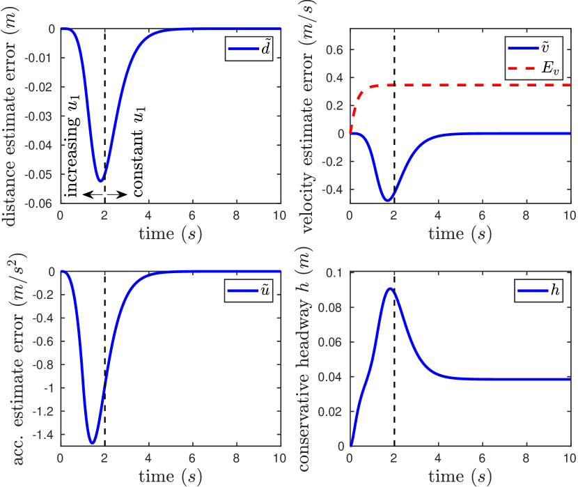
Figure 2: Performance of Estimator and conservative behavior of Control law when leader vehicle accelerates.

In the deceleration scenario, which closely resembles the acceleration scenario, the lead vehicle is programmed to decelerate for six seconds while adhering to the constraints defined by (20), subsequently, the vehicle maintains a constant velocity. The system starts with communication and ideal headway distance conditions. As demonstrated in Fig. 3, when the lead vehicle brakes, the estimator quickly converges to the origin while ensuring safety ($h>0$).

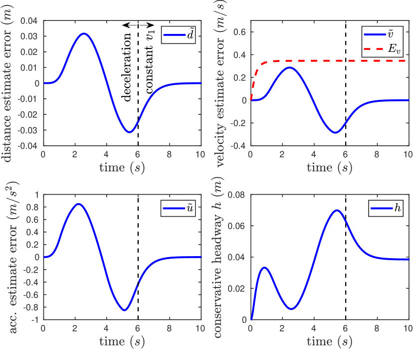
Figure 3: Performance of Estimator and conservative behavior of Control law when leader vehicle decelerates.

Another important scenario involves the lead vehicle undergoing constant acceleration or deceleration with a fixed jerk ($u_{j}$). Fig. 4 displays the system’s performance when subjected to $u_{j}{=}0.5$ m/s³, starting from rest and with an ideal headway distance. As derived in (15), the system converges to $\tilde{d}^{*}=0.0208$ m, $\tilde{v}^{*}=0.187$ m/s, $\tilde{u}^{*}=0.5416$ m/s² and $h^{*}=0.593$ m.

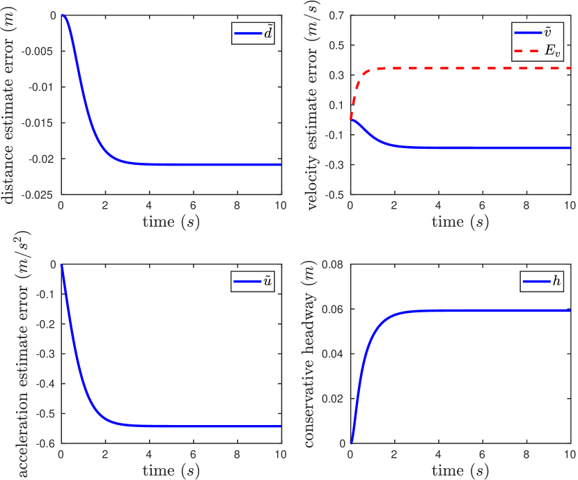
Figure 4: Performance of Estimator and conservative behavior of Control law for constant leader vehicle jerk $u_{j}$.

It is crucial to note that, for all the scenarios discussed in this section, the results show that the velocity and acceleration estimation errors satisfy $E_{v}\geq\tilde{v}_{1}$ and $E_{u}\geq\tilde{u}_{1}$ even under extreme conditions. Furthermore, while all the presented scenarios commence with an ideal headway distance, this is not a requirement. Any headway greater than the ideal distance has been proven to converge.

IV-B String Stability

String stability is a critical performance measure for ACC systems. It ensures that disturbances like sudden braking or acceleration do not propagate through the platoon, causing potential accidents or traffic congestion. In a string-stable ACC system, the amplitude of the sinusoidal velocity should decrease as it progresses from the lead vehicle to the end of the platoon. Fig. 5 demonstrates the performance of the proposed control law design in a four-vehicle platoon consisting of one lead vehicle and three autonomous vehicles. The diminished amplitude of the velocity plots (compared to the lead vehicle), as it advances toward the end, verifies the control law’s string stability. The designed controller inherently ensures string stability, while the magnitude of the string stability gain depends on the eigenvalues of the estimator state matrix $A$.

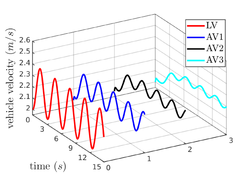
Figure 5: String stability in a four-vehicle platoon under ACC framework.

IV-C Connected Cruise Control

Connected Cruise Control is an equivalent of ACC, where vehicles have the ability to communicate their states. ACC designs are communication-independent and usually exhibit no performance improvements when employed in CCC applications, making them equivalent to scenarios without communication. However, estimator-based control laws can utilize communication to initialize estimator states, and the control design based on these estimated states should ideally perform equal to or better than the no-communication scenario.

The proposed control law’s performance depends on the upper bound of the estimated error and can demonstrate improvements when this upper bound is reduced. In the absence of communication noise and delay, communication with the lead vehicle is equivalent to a zero upper bound on the estimated error. Combining this with the adaptive error dynamics proposed in Section III-D is expected to enhance the CCC system’s performance. The system’s performance was compared in the presence and absence of communication when subjected to $u_{j}=0.5m/s^{3}$, starting from rest with an ideal headway distance. Fig. 6(a) illustrates the evolution of the estimation error upper bound in a CCC system that communicates every two seconds and compares the performance of the proposed controller under constant error bound and adaptive error bound. Fig. 6(b) illustrates the evolution of the time headway and highlights the superiority of the proposed controller with adaptive error dynamics compared to the constant error bound in a CCC application. The conservative behavior diminishes immediately after communication as the error bound approaches zero, then gradually increases and converges to the derived equilibrium point as the error accumulates.

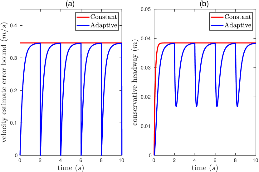
Figure 6: (a) Evolution of estimation error bound and (b) Comparison of conservative headway for fixed and adaptive estimation error in Connected Cruise Control system that communicates every 2 seconds.

IV-D Real-World Performance Evaluation

In order to assess the feasibility and verify the performance and efficacy of the proposed controller, evaluations are conducted within a physically accurate simulation environment. This section presents the dynamic evolution of various system states for a specific scenario in both MATLAB and AirSim simulators and highlights the differences between the results of the two platforms. As an open-source platform, AirSim addresses the need to bridge the gap between simulation and reality, offering a powerful tool for autonomous vehicle development. AirSim provides high-fidelity physical and visual simulation, allowing algorithm and controller development against the simulator and seamless deployment on vehicles without modification. It includes essential components such as environment and vehicle models, a physics engine, sensor models, rendering interfaces, public APIs, and an interface layer for vehicle firmware. Leveraging the power of the Unreal Engine [22], it emulates sensors like vision cameras and LiDARs, providing a realistic perception environment. The vehicle model in AirSim encompasses essential dynamics parameters such as mass, inertia, drag coefficients, friction coefficients, and restitution, enabling the physics engine to compute rigid body dynamics accurately. Additionally, the environment model incorporates crucial aspects such as gravity, air density, air pressure, and the magnetic field. The physics engine incorporated in AirSim enables real-time hardware-in-the-loop (HITL) simulations, operating at a high frequency to accurately emulate vehicle dynamics. Overall, AirSim’s combination of high-fidelity simulation, seamless integration with actual vehicles, and rich feature set make it an excellent choice for testing autonomous vehicle control algorithms [18].

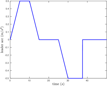
Figure 7: Leader acceleration for real-world performance evaluation.

We analyze a platoon of four vehicles operating in the absence of inter-vehicle communication. The platoon is structured such that the lead vehicle drives with the acceleration illustrated in Fig. 7, and the three other autonomous vehicles operate under the proposed controller. AirSim neighborhood environment is used with all vehicles using a custom low-level controller to match the desired throttle for the corresponding input accelerations. Additionally, The vehicles have a LiDAR sensor to sense the distance from the vehicle or obstacle ahead. The snapshot of the AirSim environment at different timestamps throughout the experiment is presented in Fig. 9.

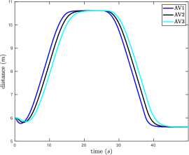
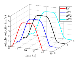
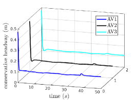
(a)	(b)	(c)
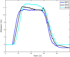
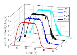
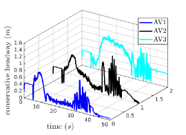
(d)	(e)	(f)

Figure 8: Evolution of distance, vehicle velocity, and conservative headway over time when leader vehicle follows the acceleration curve shown in Fig. 7 in MATLAB (a, b, c) and AirSim (d, e, f) environments.

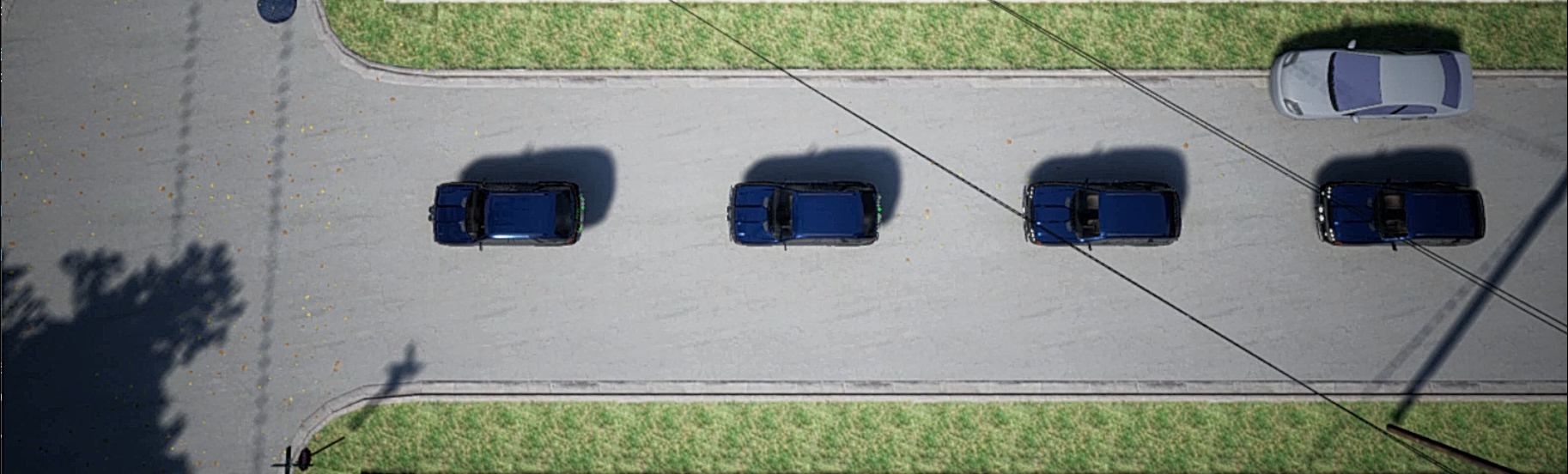
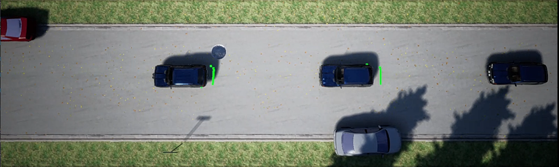
(a) $t=0$ sec.

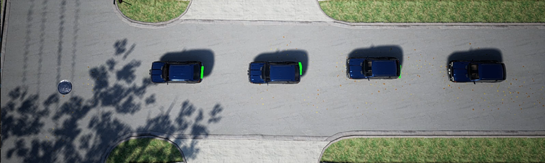
(b) $t=25$ sec.

(c) $t=50$ sec.

Figure 9: Snapshot of AirSim environment at (a) start of the experiment, (b) $t=25$ sec, and (c) end of the experiment.

Fig. 9 (a) shows the starting state of the experiment with all the vehicles at rest separated by a distance of $6$ m. The state of the experiment at $25$ sec, when all the vehicles are at a speed of about $5$ m/sec and are separated by a distance more than $10.6$ m, is shown in Fig. 9 (b). The end of the experiment, when all the vehicle comes to rest, is displayed by Fig. 9 (c). The parameters employed for the controller and estimator are $g_{1}{=}{-9}$, $g_{2}{=}{-26}$, $g_{3}{=}{-24}$, $E_{v}{=}1.0$ m/s, $E_{u}{=}1.0$ m/s², and $\beta(x){=}x$. The state matrix $A$ exhibits Hurwitz properties with these values, featuring eigenvalues of $[{-2},{-3},{-4}]$.

Upon performing the calculations, all the autonomous vehicles are expected to stop at a distance of $5.612$ m from the preceding vehicle while maintaining a conservative headway $h>0$ throughout the experiment. The evolution of key states, such as distance, vehicle velocity, and conservative headway is presented in Fig. 8 (a,b,c) for MATLAB simulation for the system dynamics described in (1). It is essential to note that this dynamics model does not account for disturbances arising from factors such as friction, air drag, and noise sensor input. Therefore the obtained results align with the calculations and are considered an ideal response. The AirSim environment model and physics engine incorporate external and internal factors, resulting in deviations from the ideal (MATLAB) response. Fig. 8 (d) shows the distance readings recorded by the LiDAR of autonomous vehicles. Due to real-world factors like friction in AirSim, vehicles cannot maintain very low speeds, preventing them from achieving the desired safe distance from the preceding vehicle. This difference is evident from the plots in Fig. 8 (a), where, at both the start and end of the experiment, the vehicle models in MATLAB manage to maintain very low velocities to achieve distances close to safe distance limit $d_{r}$. The autonomous vehicles AV1, AV2, and AV3 in MATLAB converge to $5.6102$ m, $5.6103$ m and $5.6105$ m, respectively, achieving the desired distance with a 2mm error. This error is negligible and is caused by integration errors in the simulations. However, attaining such small velocities is unfeasible for vehicles in the AirSim environment, leading AV1, AV2, and AV3 to stop at $5.548$ m, $5.5465$ m, and $5.9357$ m, respectively, as shown in Fig. 8 (d). MATLAB vehicle model employs a continuous time controller, yielding smooth velocity curves as depicted in Fig. 8 (b). In contrast, the AirSim vehicle models implement a discrete-time controller derived from the proposed continuous time controller. The inherent discretization of the controller, combined with the influence of various environmental factors, introduces disturbances into the system, evident in Fig. 8 (e). Emphasizing safety as the most critical requirement in cruise control applications, Fig. 8 (f) validates the controller’s ability to uphold safety standards despite the presence of noise and disturbance in the system. The minimum headway recorded for the three autonomous vehicles is $0.0125$ m, $0.0104$ m, and $0.0155$ m, respectively, indicating that the system successfully maintains a conservative response. The conservative headway for the three autonomous vehicles converges to $0.0480$ m, $0.0465$ m, and $0.4357$ m, respectively at the end of the experiment compared to $0.1$ m for MATLAB. It is possible to further improve the conservative response of the controller towards different factors by incorporating them in the dynamics and following the calculations as presented in Section III.

Videos of the experiments presented in this section can be found in the accompanying video for the article, available at
https://vimeo.com/849612069/60563a96f7

The results obtained through the AirSim simulation experiment substantiate the applicability and practical viability of the proposed controller in real-world scenarios. The comprehensive evaluation demonstrates the controller’s safety-critical performance and seamless compatibility with low-level controllers, underscoring the controller’s potential for deployment in adaptive cruise control applications.

V Conclusions

In this article, we have designed an estimator and the associated safety-critical controller for Adaptive Cruise Control (ACC) systems, incorporating adaptive error dynamics to further enhance controller performance. The controller’s design utilizes Control Lyapunov Functions (CLFs) and Control Barrier Functions (CBFs) to maintain system safety and stability in the presence of potential estimation errors. The proposed design is guaranteed to converge the system to a fixed conservative bias while maintaining string stability against fluctuations in the lead vehicle’s velocity, even during time-varying acceleration. We have successfully showcased the effectiveness of this estimator-controller framework in scenarios with and without vehicle-to-vehicle (V2V) communication. Our proposed design capably estimates the states of the preceding vehicle, allowing for the effective operation of autonomous vehicles within a safe region. The robustness and safety performance of our solution was further validated through physics engine-based simulations that demonstrated the practical viability of the proposed control framework under realistic environmental conditions.

We identify several promising avenues for future research. These include addressing noise factors in the safety-critical controller design, such as communication delays, input lags, and packet dropouts. Moreover, exploring the impact of time-varying delays and sensor noise on the estimator design could further enhance its performance and robustness in real-world applications.

Appendix

This appendix section provides some important calculations required in the controller and estimator design. Section V-A presents the necessary conditions for the estimator state matrix to be Hurwitz, and Section V-B derives one possible solution to (24).

V-A Estimator Design

This section presents the bounds on estimator gain variables $g_{1},g_{2}$, and $g_{3}$, given that the estimator state matrix $A$ in (4) is Hurwitz. For a $3\times 3$ matrix to be Hurwitz, the real part of the roots of the characteristic equation must be negative, i.e., $Re(\lambda_{i})<0,\,i=1,2,3$. The characteristic equation for the state matrix $A$ is given by:

$$\lambda^{3}-g_{1}\lambda^{2}-g_{2}\lambda-g_{3}=0=(\lambda-\lambda_{1})(\lambda-\lambda_{2})(\lambda-\lambda_{3})$$

Upon simplification, the following relations are obtained:

$$g_{1} =\lambda_{1}+\lambda_{2}+\lambda_{3}$$

$$g_{2} =-(\lambda_{1}\lambda_{2}+\lambda_{1}\lambda_{3}+\lambda_{2}\lambda_{3})$$

$$g_{3} =\lambda_{1}\lambda_{2}\lambda_{3}$$

A cubic polynomial can either have three real roots or have one real root and two complex conjugate roots (with $\lambda_{2}=\bar{\lambda}_{3}$). In both cases, given that $Re(\lambda_{i})<0$, $\lambda_{2}+\lambda_{3}\in\mathbb{R}^{-}$ and $\lambda_{2}\lambda_{3}\in\mathbb{R}^{+}$. Using these properties, the bounds on estimator gain variables are derived as:

$$g_{1},g_{2},g_{3}\in\mathbb{R}^{-}$$ (31)

This is a necessary condition for the state matrix $A$ to be Hurwitz.

V-B Error Dynamics Derivation

To analyze (24), let us define $\gamma$ as:

$$\gamma(b)=\frac{a(E_{u}+g_{2}\tilde{d})-\beta(ab)}{a-b};\;b\in\mathbb{R}^{+}-\{a\}$$ (32)

As the exact value of b is unavailable and only the upper and lower bounds are known, the evolution of $\gamma$ is analyzed against $b$:

$$\frac{\delta\gamma}{\delta b} =\frac{-a(a-b)\dot{\beta}(ab)+a(E_{u}+g_{2}\tilde{d})-\beta(ab)}{(a-b)^{2}}$$

$$=\frac{a(E_{u}+g_{2}\tilde{d}-a\dot{\beta}(ab))-\beta(ab)+ab\dot{\beta}(ab)}{(a-b)^{2}}$$ (33)

To derive a solution independent of $b$, we choose the class $\mathcal{K}$ function as a linear function, i.e., $\beta(x)=\bar{\beta}x$. This simplifies the above calculations as follows:

$$\frac{\delta\gamma}{\delta b}=\frac{a(E_{u}+g_{2}\tilde{d}-a\bar{\beta})}{(a-b)^{2}}$$ (34)

This implies that $\gamma$ is constant if $a=0$ or $E_{u}+g_{2}\tilde{d}=a\bar{\beta}$, monotonously increasing if $E_{u}+g_{2}\tilde{d}>a\bar{\beta}$ and monotonously decreasing if $E_{u}+g_{2}\tilde{d}<a\bar{\beta}$.
Therefore (24) is further simplified as $\dot{\epsilon}=\gamma(b)=a\bar{\beta}=E_{u}+g_{2}\tilde{d}$ if $E_{u}+g_{2}\tilde{d}=a\bar{\beta}$, and $\dot{\epsilon}=\gamma(b)=0$ if $a=0$. Similarly, for $E_{u}+g_{2}\tilde{d}>a\bar{\beta}$, we obtain:

$$\begin{cases}\dot{\epsilon}=\gamma(b_{M})\;;&a>b\\ \dot{\epsilon}=\gamma(a^{+})\to-\infty\;;&a<b\\ \dot{\epsilon}=0\;;&a=b\end{cases}$$ (35)

where $b_{M}=\epsilon-v_{m}$ is the upper bound on $b$ with $v_{m}$ as the lower bound on $\tilde{v}_{1}$. Similarly, when $E_{u}+g_{2}\tilde{d}<a\bar{\beta}$, we have $\dot{\epsilon}=0$. One possible solution that satisfies these bounds and is independent of $b$ is calculated as in (25).

References

- [1] Z. Wang, G. Wu, and M. J. Barth, “A review on cooperative adaptive cruise control (cacc) systems: Architectures, controls, and applications,” in 2018 21st International Conference on Intelligent Transportation Systems (ITSC), 2018, pp. 2884–2891.
- [2] G. Orosz, “Connected cruise control: modelling, delay effects, and nonlinear behaviour,” Vehicle System Dynamics, vol. 54, no. 8, pp. 1147–1176, 2016.
- [3] T. G. Molnar, A. Alan, A. K. Kiss, A. D. Ames, and G. Orosz, “Input-to-state safety with input delay in longitudinal vehicle control,” IFAC-PapersOnLine, vol. 55, no. 36, pp. 312–317, 2022.
- [4] F. Acciani, P. Frasca, A. Stoorvogel, E. Semsar-Kazerooni, and G. Heijenk, “Cooperative adaptive cruise control over unreliable networks: an observer-based approach to increase robustness to packet loss,” in 2018 European Control Conference (ECC), 2018, pp. 1399–1404.
- [5] Z. Wang, Y. Gao, C. Fang, L. Liu, S. Guo, and P. Li, “Optimal connected cruise control with arbitrary communication delays,” IEEE Systems Journal, vol. 14, no. 2, pp. 2913–2924, 2020.
- [6] F. Di Rosa, A. Petrillo, J. Ploeg, S. Santini, and T. P. van der Sande, “Sliding mode acceleration estimation for safe vehicular cooperative adaptive cruise control,” in 2022 IEEE 25th International Conference on Intelligent Transportation Systems (ITSC), 2022, pp. 2028–2033.
- [7] L. Wu, S. Wen, Y. He, Q. Zhou, and Z. Lu, “Observer-based cooperative adaptive cruise control of vehicular platoons with random network access,” in IEEE Intelligent Vehicles Symposium (IV), 2018, pp. 232–237.
- [8] A. Wasserburger, A. Schirrer, N. Didcock, and C. Hametner, “A probability-based short-term velocity prediction method for energy-efficient cruise control,” IEEE Transactions on Vehicular Technology, vol. 69, no. 12, pp. 14 424–14 435, 2020.
- [9] Y. Lin, J. McPhee, and N. L. Azad, “Comparison of deep reinforcement learning and model predictive control for adaptive cruise control,” IEEE Transactions on Intelligent Vehicles, vol. 6, no. 2, pp. 221–231, 2021.
- [10] M. K. Rout, D. Sain, S. K. Swain, and S. K. Mishra, “Pid controller design for cruise control system using genetic algorithm,” in 2016 International Conference on Electrical, Electronics, and Optimization Techniques (ICEEOT), 2016, pp. 4170–4174.
- [11] B. Sakhdari and N. L. Azad, “Adaptive tube-based nonlinear mpc for economic autonomous cruise control of plug-in hybrid electric vehicles,” IEEE Transactions on Vehicular Technology, vol. 67, no. 12, pp. 11 390–11 401, 2018.
- [12] Z. Wang, S. Jin, L. Liu, C. Fang, M. Li, and S. Guo, “Design of intelligent connected cruise control with vehicle-to-vehicle communication delays,” IEEE Transactions on Vehicular Technology, vol. 71, no. 8, pp. 9011–9025, 2022.
- [13] A. D. Ames, X. Xu, J. W. Grizzle, and P. Tabuada, “Control barrier function based quadratic programs for safety critical systems,” IEEE Transactions on Automatic Control, vol. 62, no. 8, pp. 3861–3876, 2017.
- [14] Y. Wang and X. Xu, “Observer-based control barrier functions for safety critical systems,” in 2022 American Control Conference (ACC), 2022, pp. 709–714.
- [15] A. Alan, T. G. Molnar, E. Daş, A. D. Ames, and G. Orosz, “Disturbance observers for robust safety-critical control with control barrier functions,” IEEE Control Systems Letters, vol. 7, pp. 1123–1128, 2023.
- [16] I. Karafyllis, D. Theodosis, and M. Papageorgiou, “Nonlinear adaptive cruise control of vehicular platoons,” International Journal of Control, vol. 96, no. 1, pp. 147–169, 2023.
- [17] C. R. He and G. Orosz, “Safety guaranteed connected cruise control,” in 2018 21st International Conference on Intelligent Transportation Systems (ITSC), 2018, pp. 549–554.
- [18] S. Shah, D. Dey, C. Lovett, and A. Kapoor, “Airsim: High-fidelity visual and physical simulation for autonomous vehicles,” in Field and Service Robotics, 2017. [Online]. Available: https://arxiv.org/abs/1705.05065
- [19] D. Swaroop, J. Hedrick, C. C. Chien, and P. Ioannou, “A comparision of spacing and headway control laws for automatically controlled vehicles1,” Vehicle System Dynamics, vol. 23, no. 1, pp. 597–625, 1994.
- [20] H. K. Khalil, Nonlinear systems, 2nd ed. Upper Saddle River, NJ 07458: Prentice-Hall, 2011.
- [21] P. L. L. Rodman, Algebraic Riccati equations, 2nd ed. Oxford University Press, 1995.
- [22] G. E. Brian Karis, “Real shading in unreal engine 4 by,” in Physically Based Shading Theory Practice, 2013.