Novel high-frequency gravitational waves detection with split cavity

Abstract

Gravitational waves can generate electromagnetic effects inside a strong electric or magnetic field within the Standard Model and general relativity. Here we propose using a quarterly split cavity and LC-resonance circuit to detect a high-frequency gravitational wave from 0.1 MHz to GHz. We perform a full 3D simulation of the cavity’s signal for sensitivity estimate. Our sensitivity depends on the coherence time scale of the high-frequency gravitational wave sources and the volume size of the split cavity. We discuss the resonant measurement schemes for narrow-band gravitational wave sources and also a non-resonance scheme for broadband signals. For a meter-sized split cavity under a 14 Tesla magnetic field, the LC resonance enhanced sensitivity to the gravitational wave strain is expected to reach $h\sim 10^{-20}$ around $10$ MHz.

I introduction

LIGO and Virgo, the ground base interferometers have directly observed the gravitational waves(GWs) Abbott et al. (2016) , which started the era of GW astronomy. Along with electromagnetic waves from another long-range interaction, now we can observe the universe from both spectra. The central focus of the current GW experiment is from Hz to kHz with ground-based experimentsHild et al. (2011); Punturo et al. (2010); Abbott et al. (2017). The other gravitational waves proposal, from high to ultra-low frequency, includes space-basedAmaro-Seoane et al. (2017); Yagi and Seto (2011), moon-basedHarms et al. (2021); van Heijningen et al. (2023), laser/atom interferometersBadurina et al. (2020); Abe et al. (2021); El-Neaj et al. (2020), pulsar timing arraysArzoumanian et al. (2020); Janssen et al. (2015), and CMB observationsNamikawa et al. (2019); Abazajian et al. (2020), etc.

If we go into the other end of the gravitational wave spectra, the higher frequency, various interesting proposals, and detectors have already been put forth, including superconducting ringsAnandan and Chiao (1982), microwave and optical cavitiesMensky and Rudenko (2009); Caves (1979); Pegoraro et al. (1978a, b); Reece et al. (1984, 1982); Ballantini et al. (2005); Bernard et al. (2002, 2001); Ballantini et al. (2003); Cruise (2000); Cruise and Ingley (2005, 2006), interferometers.Ackley et al. (2020); Bailes et al. (2019); Akutsu et al. (2008); Chou et al. (2017); Nishizawa et al. (2008), optically levitated sensorsAggarwal et al. (2020), mechanical resonatorsGoryachev et al. (2014); Goryachev and Tobar (2014); Aguiar (2011); Gottardi et al. (2007), and detectors based on the inverse-Gertsenshtein effectGertsenshtein (1962); Braginskii et al. (1973) and the magnon modesIto et al. (2020); Ito and Soda (2022)( e.g. see Aggarwal et al. (2021) for a comprehensive review), and some very recent novel proposals Bringmann et al. (2023); Domcke and Garcia-Cely (2021); Barrau et al. (2023); Vadakkumbatt et al. (2021); Howl and Fuentes (2021); Goryachev et al. (2021) . Those experiments are designed to be tabletop or room-size, to match the smaller wavelength. However, there are still orders of magnitudes in gravitational wave amplitude strains for experiments to meet theory prediction.

Recent progress has been made that existing axion search experiments can already cast the limits on the high-frequency gravitational waves sensitivities Domcke et al. (2022); Berlin et al. (2022). In this work, we propose a new way to detect high-frequency gravitational waves from kHz to GHz, a design with a split cavity as a capacitor and readout LC circuit, different yet resembling those axion detection schemes, such as cavity-based ADMXBartram et al. (2021), non-cavity ABRACADABRAHenning et al. (2018); Salemi (2019), SHAFTGramolin et al. (2021) and DM-RadioBrouwer et al. (2022); Silva-Feaver et al. (2017). The quarterly split cavity roughly matches the quadruple shape of the gravitational wave oscillations and does not need to resemble the geometric rigidity of a closed cavity. Its frequency response does not need to develop a sharp peak at the resonant frequency, thus it can also be used in a broad-band measurement. The high-frequency gravitational wave detection proposal here employs a similar readout and capacitor-based design, with the axion detection RELEAPDuan et al. (2023). For most of the proposed gravitational wave sources, signals do not have a high coherent factor, which is the crucial difference from the axion oscillating background. Here we discuss different signal processing schemes and show both the exclusion limits for the LC-resonant scheme, targeting coherent narrowband sources, and the non-resonant broadband scheme for transient signals.

We organize the rest of the paper as follows: in section II, we show the theoretical calculation of the gravitational wave-induced electromagnetic current, especially the result for incoming gravitational waves in arbitrary angles; in section III, we discuss the electromagnetic solution with the split cavity and the numerical simulation with COMSOL; in section IV, we show the sensitivity reach of our proposal, based on the numerical simulation, and comparing them with the other limits with broadband axion detectors.

II Gravitational Wave Electrodynamics

Throughout this paper, we use Heaviside units with $\hbar=c=1$, $\eta_{\mu\nu}=\mathrm{diag}(-+++)$, work to leading order in $|h_{\mu\nu}|$, and raise indices with $\eta^{\mu\nu}$.

We start with the Lagrangian for the Inverse Gertsenshtein effect, which is present in the Standard model Ejlli et al. (2019):

$$S=\int d^{4}x\sqrt{-g}\left(-\frac{1}{4}g^{\mu\alpha}g^{\nu\beta}F_{\mu\nu}F_{\alpha\beta}\right)$$

Then we can expand the metric to the leading order in h, as below

$$S\supset-\frac{1}{2}\int d^{4}xj_{\mathrm{eff}}^{\mu}A_{\mu}$$

where

$$j_{\mathrm{eff}}^{\mu}\equiv\partial_{\nu}\left(\frac{1}{2}hF^{\mu\nu}+h_{\alpha}^{\nu}F^{\alpha\mu}-h_{\alpha}^{\mu}F^{\alpha\nu}\right)$$

Here we employ the result from Berlin et al. (2022) with a most positive metric notation. For convenience, we can write out $R_{\mu\nu\rho\sigma}$ in the TT frame,

$$h_{00}=-\omega_{g}^{2}h_{ab}^{\mathrm{TT}}x^{a}x^{b}\left[\frac{i}{-\omega_{g}z}+\frac{1-e^{-i\omega_{g}z}}{\left(\omega_{g}z\right)^{2}}\right]$$

$$h_{ij}=\omega_{g}^{2}\left[\left(\delta_{iz}h_{ja}^{\mathrm{TT}}+\delta_{jz}h_{ia}^{\mathrm{TT}}\right)zx^{a}-h_{ij}^{\mathrm{TT}}z^{2}-\delta_{iz}\delta_{jz}h_{ab}^{\mathrm{TT}}x^{a}x^{b}\right]\left[-\frac{1+e^{-i\omega_{g}z}}{\left(\omega_{g}z\right)^{2}}-2i\frac{1-e^{-i\omega_{g}z}}{\left(\omega_{g}z\right)^{3}}\right]$$

$$h_{0i}=-\omega_{g}^{2}\left(h_{ia}^{\mathrm{TT}}zx^{a}-\delta_{iz}h_{ab}^{\mathrm{TT}}x^{a}x^{b}\right)\left[\frac{-i}{2\omega_{g}z}-\frac{e^{-i\omega_{g}z}}{\left(\omega_{g}z\right)^{2}}-i\frac{1-e^{-i\omega_{g}z}}{\left(\omega_{g}z\right)^{3}}\right],$$

The components of $h_{ij}^{\mathrm{TT}}$ can then take the following explicit forms

$$\left.h_{\rho\rho}^{\mathrm{TT}}\right|_{\mathbf{r}=0}=-e^{i\omega_{g}t}\left(-h^{+}\left(\sin^{2}\left(\phi-\phi_{h}\right)-\cos^{2}\left(\phi-\phi_{h}\right)\cos^{2}\theta_{h}\right)+2h^{\times}\cos\theta_{h}\cos\left(\phi-\phi_{h}\right)\sin\left(\phi-\phi_{h}\right)\right),$$

$$\left.h_{\rho\phi}^{\mathrm{TT}}\right|_{\mathbf{r}=0}=-e^{i\omega_{g}t}\left(-h^{+}\left(1+\cos^{2}\theta_{h}\right)\sin\left(\phi-\phi_{h}\right)\cos\left(\phi-\phi_{h}\right)+h^{\times}\cos\left(2\left(\phi-\phi_{h}\right)\right)\cos\theta_{h}\right),$$

$$\left.h_{\rho z}^{\mathrm{TT}}\right|_{\mathbf{r}=0}=e^{i\omega_{g}t}\left(h^{+}\cos\theta_{h}\sin\theta_{h}\cos\left(\phi-\phi_{h}\right)+h^{\times}\sin\theta_{h}\sin\left(\phi-\phi_{h}\right)\right),$$

$$\left.h_{\phi z}^{\mathrm{TT}}\right|_{\mathbf{r}=0}=-e^{i\omega_{g}t}\left(h^{+}\cos\theta_{h}\sin\theta_{h}\sin\left(\phi-\phi_{h}\right)-h^{\times}\sin\theta_{h}\cos\left(\phi-\phi_{h}\right)\right),$$

$$\left.h_{zz}^{\mathrm{TT}}\right|_{\mathbf{r}=0}=-e^{i\omega_{g}t}h^{+}\sin^{2}\theta_{h}.$$

We here follow the notation in Domcke et al. (2022); Berlin et al. (2022), and further explicitly calculate out the gravitational wave effective current with incoming gravitational waves in arbitrary angles. Let us take the background magnetic field to be static, spatially uniform, and pointing along the $+\hat{z}$ direction in the TT frame, $\mathbf{B}_{0}=B_{0}\hat{z}$, $j^{\mu}_{\mathrm{eff}}$ can be determined by direct calculation,

$$j^{0}_{\mathrm{eff}} =\frac{B_{0}(-1+e^{\kappa})w_{g}^{2}(\mathrm{k_{1}b_{2}-b_{1}k_{2}})}{-\kappa}$$ (1)

$$j_{\mathrm{eff}}^{\rho} =\frac{1}{2\kappa^{3}}B_{0}w_{g}^{2}(2+\kappa)\left(-2-2e^{\kappa}(-1+\kappa)+\kappa^{2}\right)\mathrm{b_{2}}+\frac{1}{\kappa^{2}}B_{0}w_{g}^{2}\left(1+e^{\kappa}(-1+\kappa)\right)\rho h^{\mathrm{TT}}_{\rho\phi}|_{\mathbf{r}=0}$$

$$-\frac{1}{2\kappa^{4}}iB_{0}w_{g}^{3}\left(-6+e^{\kappa}(6-4\kappa)-2\kappa+\kappa^{2}+\kappa^{3}\right)(\mathbf{b}\cdot\mathbf{r})\mathrm{k_{2}}$$

$$j_{\mathrm{eff}}^{\phi} =\frac{B_{0}w_{g}^{2}\left(1+e^{\kappa}(-1+\kappa)\right)\rho}{\kappa^{2}}h^{\mathrm{TT}}_{\phi\phi}|_{\mathbf{r}=0}+\frac{iB_{0}w_{g}^{3}\left(-6+e^{\kappa}(6-4\kappa)-2\kappa+\kappa^{2}+\kappa^{3}\right)(\mathbf{b}\cdot\mathbf{r})\mathrm{k_{1}}}{2\kappa^{4}}$$

$$-\frac{B_{0}w_{g}^{2}(2+\kappa)\left(-2-2e^{\kappa}(-1+\kappa)+\kappa^{2}\right)\mathrm{b_{1}}}{2\kappa^{3}}$$

$$j_{\mathrm{eff}}^{z} =\frac{B_{0}w_{g}^{2}\left(1+e^{\kappa}(-1+\kappa)\right)\rho h^{\mathrm{TT}}_{\phi z}|_{\mathbf{r}=0}}{\kappa^{2}}$$

Where $\mathbf{b}=(b_{1},b_{2},b_{3}),b_{j}=r_{i}h^{\mathrm{TT}}_{ij}|_{\mathbf{r}=0},\mathbf{k}=(k_{1},k_{2},k_{3})=(\sin\theta_{h}\cos(\phi-\phi_{h}),-\sin\theta\sin(\phi-\phi_{h}),\cos\theta_{h}),\mathbf{r}=(\rho,\phi,z),\kappa=-i\mathbf{k.r}$.

If we take the incoming gravitational waves direction as the z-direction, aligned with the magnetic field, and assume cylindrical symmetry with cylindrical coordinates, the GW effective current can be simplified as:

$$j_{\mathrm{eff}}^{\mu}=-\frac{B_{0}\omega_{g}^{2}r}{6\sqrt{2}}e^{i\omega_{g}t}\left(0,ie^{-2i\phi}h_{+2}-ie^{2i\phi}h_{-2},e^{-2i\phi}h_{+2}+e^{2i\phi}h_{-2},0\right)\times f\left(\omega_{g}z\right),$$ (2)

where $f(x)\equiv-3-6ix^{-1}-12e^{-ix}x^{-2}-12i\left(1-e^{-ix}\right)x^{-3}$ is a dimensionless function with $\lim_{x\rightarrow 0}f(x)=1$ and $\lim_{x\rightarrow\infty}f(x)=-3$. GW helicity components are defined as $h_{\pm 2}\equiv\left(h_{+}\pm ih_{\times}\right)/\sqrt{2}$. In the SI unit, we can replace $B_{0}$ with $B_{0}/\left(\mu_{0}c^{2}\right)$ above in $j_{\text{eff}}^{\mu}$. We illustrate $j_{\text{eff}}$ in the x-y plane in Fig.1.

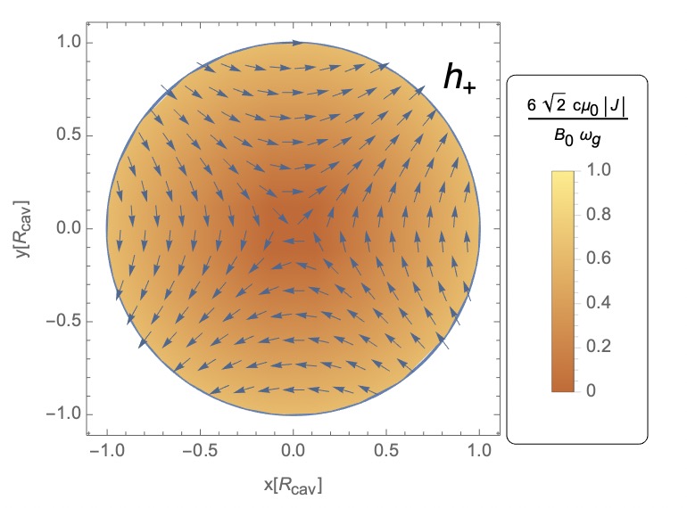
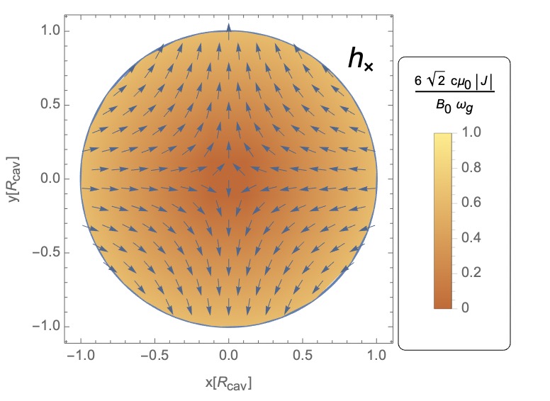
Figure 1: We plot the $j_{\text{eff}}$ with only cross/plus mode at z=0 in x-y plane in Eq.2. The arrows denote the direction of $j^{\mu}$ and the different color scales represent the magnitude.

III Solutions with split cavity

III.1 Cylindrical modes inside a solenoid

A solenoid is the common form of an experimental strong $B$-field. We would first find out the induced electromagnetic modes under the symmetries of a solenoid, and design the readout apparatus accordingly.

The eigenmode solutions inside a closed cylinder of radius $R_{\rm cav}$ and finite length $L_{\rm cav}$, under ideal conductor boundary conditions, are classified into resonant transverse magnetic (TM) and transverse electric (TE) modes Hill (2009). The TM modes are:

$$E_{r}^{\pm} = -\left[{A_{+}\sin m\phi\atop A_{-}\cos m\phi}\right]\frac{k_{z}}{\omega_{mnp}^{2}-k_{z}^{2}}\sin(k_{z}z)J^{\prime}_{m}(r\gamma_{mn})\gamma_{mn},$$ (3)

$$E_{\phi}^{\pm} = -\left[{A_{+}\cos m\phi\atop-A_{-}\sin m\phi}\right]\frac{k_{z}}{\omega_{mnp}^{2}-k_{z}^{2}}\sin(k_{z}z)\frac{m}{r}J_{m}(r\gamma_{mn}),$$ (4)

$$E_{z}^{\pm} = \left[{A_{+}\sin m\phi\atop A_{-}\cos m\phi}\right]J_{m}(\gamma_{mn}r)\cos(k_{z}z),$$ (5)

where $\omega_{mnp}$ is the frequency at the resonant mode. The $\pm$ at the $E$-fields correspond to the upper/lower component in the brackets, $A_{\pm}$ are constants that are determined by normalization condition. We have $k_{z}=\pi p/L_{\rm cav}$, $\gamma_{mn}=x_{mn}/R_{\rm cav}$, $x_{mn}$ is the $n$th zero of 1st Bessel function $J_{m}$. The mode numbers $m$ and $p$ are non-negative integers while $n$ is a positive integer. The TE_mnp modes are:

$$E_{r}^{\pm} = \left[{A_{+}\cos m\phi\atop-A_{-}\sin m\phi}\right]\sin\left(k_{z}z\right)\frac{i\omega_{mnp}}{\omega_{mnp}^{2}-k_{z}^{2}}\frac{m}{r}J_{m}(r\gamma_{mn}),$$ (6)

$$E_{\phi}^{\pm} = -\left[{A_{+}\sin m\phi\atop A_{-}\cos m\phi}\right]\frac{i\omega_{mnp}}{\omega_{mnp}^{2}-k_{z}^{2}}\sin\left(k_{z}z\right)J_{m}^{\prime}(\gamma_{mn}r)\gamma_{mn},$$ (7)

$$E_{z}^{\pm} = 0,$$ (8)

where $\gamma_{mn}=x_{mn}^{\prime}/R_{\rm cav}$, and $x_{mn}^{\prime}$ is the $n$th zero of $J^{\prime}_{m}$. Those modes are orthogonal to each other as defined in the mode bases. These modes are used later to demonstrate the spin-2 nature of the effective current.

III.2 A quarterly split cavity

In principle, any induced signal EM field can be expressed as the linear combination of the modes in Eq. 3-8. If we assume a gravitational plane wave that propagates along the cylinder’s $\hat{z}$ axis, the effective current $j_{\rm eff}$ lies in the transverse $\hat{x}-\hat{y}$ directions. The spin-2 nature of the gravitational mode is reflected by the $e^{\pm i2\phi}$ rational symmetry in Eq 2.

Taking the lowest ${\bf E}$ mode numbers, the base mode that the gravitational waves along the z direction excite is $TE_{211\pm}$ and its spatial components are given as

$$E_{r}^{\pm} = \left[{A_{+}\cos 2\phi\atop-A_{-}\sin 2\phi}\right]\sin\left(\frac{\pi z}{L_{\rm cav}}\right)\frac{i\omega_{211}}{\omega_{211}^{2}-(\frac{2\pi}{L_{\rm cav}})^{2}}\frac{2}{r}J_{2}(r\gamma_{21}),$$ (9)

$$E_{\phi}^{\pm} = -\left[{A_{+}\sin 2\phi\atop A_{-}\cos 2\phi}\right]\frac{i\omega_{211}}{\omega_{211}^{2}-(\frac{2\pi}{L_{\rm cav}})^{2}}\sin\left(\frac{\pi z}{L_{\rm cav}}\right)J_{2}^{\prime}(\gamma_{21}r)\gamma_{21},$$ (10)

$$E_{z}^{\pm} = 0,$$ (11)

and the corresponding resonant frequency is

$$\omega_{211}=\sqrt{k_{z}^{2}+\gamma_{mn}^{2}}=\sqrt{(\frac{\pi}{L_{\rm cav}})^{2}+(\frac{x^{\prime}_{21}}{R_{\rm cav}})^{2}}.$$ (12)

The vertical components $E_{\phi},E_{z}$ vanish at the closed boundary, $r=R_{cav}$. Only $E_{r}$ is non-zero and it is perpendicular to the cylindrical inner surface.

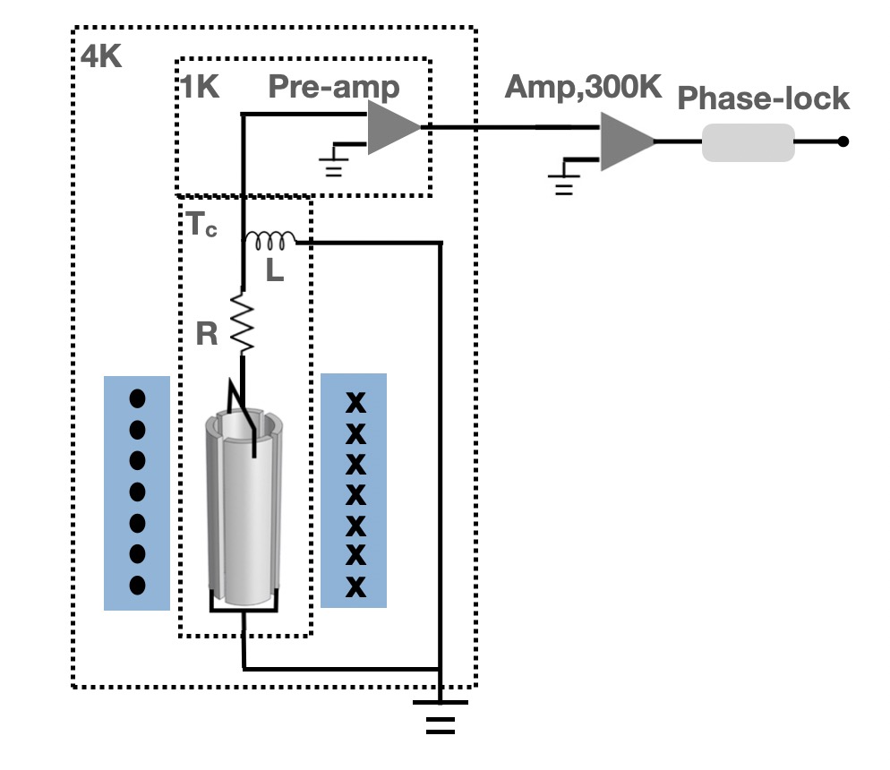
Figure 2: Split cavity: the top, bottom, and quarterly split periphery of the cylinder cavity are separated by insulation to form induction signal currents through the connection wiring. The slit angle is $3^{\circ}$ in this case. The connecting wires and amplification LC circuit are also shown.

For a given cylinder size, the optimal situation is when the signal frequency $\omega$ matches one of the TE modes’. Frequency mismatch between the signal and cavity’s eigenmodes leads to non-zero projection into higher TE modes, which may not always sum up constructively. As a consequence, efficiency loss will occur in both high-frequency and low-frequency directions: $\omega\ll\omega_{211}$ is expected to suffer major form factor suppression, and $\omega\gg{\rm min}(R_{\rm cav}^{-1},L_{\rm cav}^{-1})$ will hit the decoherence limit due to the signal photon conversion in a spatial region larger than its wavelength. The maximal conversion efficiency typically occurs near the base mode $\omega_{211}$ for the given dimensions of a cavity. Therefore, in a narrow-band setup, it favors applying frequency filtering in a neighborhood around $\omega\sim\omega_{211}$.

The electric field distribution will redistribute the electrons on the cylinder’s conductor surface, and TE₂₁₁ mode will feature in a quadruple-like distribution in the cross-section of the cylinder. We split up the cylinder in a quarterly manner so that the electron redistribution between two adjacent plates has to flow through external wiring, thus leading to a measurable current signal, as illustrated in Fig. 2. The resulting electric response does not depend on the particular narrow slit angle drastically. Note the quarterly pattern will mostly pick up the quadruple component, the plus or cross mode that aligns with the slits’ $\phi$-separation, and loses the orthogonal component that leans at a 45^∘ angle.

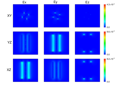
Figure 3: EM response simulation of the incoming gravitational waves $h=10^{-10}$ in the z-direction with a quarterly split cylinder $R=1$cm and $L=5$cm. The unit is $V/m$.

Splitting up the plates will cause significant deformation on the TE₂₁₁ mode. Even when the slits are narrow, their impact on the eigenmodes is noticeable, mostly through the aperture enhancement effect as in F.Harrington (2001). We performed an EM numerical simulation of the split cylinder with COMSOL package COM to obtain the electric field distribution within the cavity and then compute the corresponding electric charge distribution on the quarter-plates at different frequencies. With an LC enhancement, we do not require the cavity itself to provide narrow-band filtering. Thus in principle, the cavity does not need to resemble the geometric rigidity of a closed cavity. In other words, a split/open cavity’s frequency response does not need to develop a sharp peak at $\omega_{211}$ and it can also be used in a broad-band measurement, which we will discuss later.

The EM simulation results for the plates’ charge accumulation and effective capacitance are shown in Table 1. The set-up with the split cavity and LC circuit amplification readout is shown in 2, and the full numerical EM simulation is shown in 3. We refer to Duan et al. (2023) for more details of the cryogenic amplification readout system.

R:L = 1cm:5cm			R:L = 1m:1m
$f$ (Hz)	$C$ (pF)	$q$ (C)	$f$ (Hz)	$C$ (pF)	$q$ (C)
$10^{7}$	1.53	$2.39\times 10^{-19}$	$10^{5}$	31.05	$2.04\times 10^{-16}$
$10^{8}$	1.53	$2.39\times 10^{-18}$	$10^{6}$	31.05	$2.04\times 10^{-15}$
$10^{9}$	1.52	$2.29\times 10^{-17}$	$10^{7}$	31.05	$2.03\times 10^{-14}$

Table 1: Selected values of the cavity’s effective capacitance $C$ and the accumulated charge $q$ from EM simulations. The GW is assumed to propagate along the cavity axis with an amplitude $h_{0}=10^{-10}$ . The left and right columns show two experimental scales: a multi-center-sized cavity with $f_{211}=1.5\times 10^{10}$ Hz, and a meter-sized cavity with $f_{211}=2.1\times 10^{8}$ Hz. Notice here our working frequencies are away from the closed cavity’s resonance frequencies.

IV Sensitivity Prospects.

IV.1 Narrow-band scheme

As we discussed previously, a cavity has its optimal working frequency for signal pickup. A narrow band measurement scheme involves frequency filtering at this favored frequency range, and there are two popular ways to achieve this: (1) a high geometric quality factor of the cavity $Q_{c}$ Sikivie (1983); (2) electronic filtering with an LCR circuit Sikivie et al. (2014) with a quality factor $Q_{c}=(\omega CR_{s})^{-1}$, where $C,R_{s}$ denote the LCR’s capacitance and resistance at the resonant point. In either case, when the signal’s and the pickup’s quality factors match each other, the high pickup quality factor is capable of enhancing the output power from a monochromatic perturbation source by a factor of the order ${\cal O}(Q_{c})$. Assuming this condition could be met, the enhanced signal current is

$$I_{a}=Q_{c}\cdot q_{0}\omega\cos(\omega t),$$ (13)

where $q_{0}$ is maximal (un-enhanced) charge build-up on the plates due to the signal field, and it is derived by a surface integral of E field strength around one-quarter of the cylindrical plate’s inner surface:

$$q_{0}=\int\vec{E}\cdot{\rm d}{\vec{A}},$$ (14)

For the quadrupole configuration, this charge can be rewritten as

$$\begin{array}[]{rcl}q_{0}=\int E_{r}(\omega)\cdot dA&=&\eta_{J}\cdot\left.\frac{\pi RL}{2}E_{r}(\omega)\right|_{r=R_{\rm cav},\phi=45^{\circ}}\\ \end{array}$$ (15)

where in the first line we make use of the fact that quarter-plates have an effective capacitance $C\sim\pi L\eta_{J}(\omega)$, and $\eta_{J}$ is a form factor to account for the geometric layout of the quadruple shaped cavity. From EM simulation results in Table 1, we can evaluate $\eta_{J}$ to be $27.52\epsilon_{0}=27.52\times 8.85\text{pF/m}$ for a 1 cm³ cavity and and $1.12\epsilon_{0}\text{pF/m}$ for a 1 m³ cavity, respectively. We can estimate by $E_{r}(r=R_{0})\sim B_{0}h_{0}c(\omega_{g}R_{0})^{2}$ at the center of each plate from dimension analysis. For a GHz-frequency GW wave with a stress intensity $h\sim 10^{-20}$, we will have $E_{r}\sim 10^{-10}$ V/m for a meter scale $R_{\rm cav}=1$ m cavity for a rough dimension analysis. Due to the imperfect symmetry of our cavity, we resort to numerical simulation to evaluate the signal electric fields.

For an LCR-type of filtering as shown in Fig. 2, The $Q$-enhanced signal power at the resonance point is

$$P_{\rm sig.}=\left<{I_{a}^{2}}\right>\cdot R_{s}=\frac{(Q_{c}\omega q_{0})^{2}}{2Q_{c}\omega C}=Q_{c}\cdot\left<{q_{0}^{2}}\right>\omega~{}C^{-1},$$ (16)

where $C$ is the effective capacitance of the plates, and this power equals the maximal thermal dissipation power at the LCR circuit. With the GW estimation, we have

$$P_{\rm sig.}\sim Q_{c}\omega_{g}\frac{(\pi RLB_{0}h_{0}c)^{2}}{4\pi L\eta_{J}}=Q_{c}\omega_{g}\pi R^{2}L\frac{(B_{0}h_{0}c)^{2}}{4\eta_{J}}.$$ (17)

Here the maximal signal power is for $\omega_{g}\sim 0.1\omega_{211}$.

The signal power can be subsequently amplified and read out by cryogenic detectors. For a conceptual discussion in this work, we will not go into depth into noise discussion and only assume a thermal-noise-dominated background. At sub-GeV frequencies, the quantum noise is subdominant to amplifier noises, and a reasonable choice with modern cryogenic technique is an equivalent noise temperature at $T_{N}=0.1$ K Duan et al. (2023). This noise temperature gives the noise power of $P_{N}=k_{B}T_{N}\Delta f$, where $k_{B}$ is the Boltzmann constant, and for narrow-band filtering, we choose the bandwidth to be $\Delta f\sim\omega/(2\pi Q_{c})$. The signal-to-noise rate is then

$${\rm SNR}=\frac{P_{\rm sig.}}{k_{\rm B}T_{N}}\sqrt{\frac{\Delta{t}}{\Delta f}},$$ (18)

where $\Delta t$ is the observation time which we take to be 1 min here and we can require SNR$=3$ for a $3\sigma$ sensitivity criterion, the corresponding sensitivity on the GW stress is plotted in fig.3.

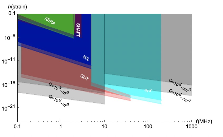
Figure 4: Projected sensitivity to the stress of a GW signal, with coherent factor Q=$10^{6}$ and $10^{3}$, corresponding to narrowband searches. For comparison, existing experimental limits from ABRACADABRAHenning et al. (2018); Salemi (2019), SHAFTGramolin et al. (2021), and the projected sensitivity from DM-RadioBrouwer et al. (2022); Silva-Feaver et al. (2017) are also shown in plot.

Note in our narrow-band scheme there is a not-small assumption that the signal should be also narrow-band in its frequency domain, in order to match that of the pickup and trigger the high-$Q$ enhancement. This requires a near monochromatic signal and a relatively long coherence time scale, at least longer than $2\pi Q_{c}/\omega$ to ring up the resonance enhancement. Typically, this indicates the narrow-band measurement scheme is best for a GW source with good coherent oscillation periodicity. There are potential candidates of such sources, for instance, the GW induced by the coherent oscillation of a light scalar field as a dark matter condensate Sun and Zhang (2021) or a superradiance cloud around Kerr black holes Brito et al. (2015), etc. For non-periodic yet coherent sources, such as transient events, we will change our plan and consider the broad-band $\Delta f\sim f$ sensitivity of the non-resonant measurement.

IV.2 Non-resonant scheme

For non-periodic transient signals, the sensitivity of our measurement can be estimated by comparing the signal-to-noise ratio within the signal’s expected time duration. In case the signal has an extended spectrum in the frequency domain, the choice of measurement bandwidth needs to account for the frequency dependence of the signal pickup.

GW-induced effective current $j_{\rm eff}$ is generated by time-variance in the metric $\partial_{t}h$, the induced current between electrodes is proportional to $\partial_{t}q\propto\partial_{t}j_{\rm eff}$, therefore our measured signal responds to $\partial_{t}^{2}h$ and should have a higher sensitivity to the high-frequency part of the GW signal spectrum. For specific sources, the shape of $\partial_{t}^{2}h$ will affect our detection efficiency: we need to choose our bandwidth to cover the frequency range where $\partial_{t}^{2}h$ maximizes.

Highly motivated high-frequency coherent GW sources include the binary mergers of primordial black holes and blackhole superradiance. For the blackhole binary merger, the emitted gravitational wave frequency is associated with the ISCO and the inspiral emission peaks at

$$f_{\rm ISCO}\simeq 4.4\text{MHz}\,\left(\frac{10^{-3}M_{\odot}}{m^{\scriptscriptstyle\textrm{PBH}}_{1}+m^{\scriptscriptstyle\textrm{PBH}}_{2}}\right)\!.$$ (19)

and we have the GW strains from the merger along the symmetry axis of the circular orbit  Maggiore (2007)

$$h_{+,\times}^{\scriptscriptstyle\textrm{PBH}}\sim 2.5\times 10^{-21}\left(\frac{10~{}\text{kpc}}{D}\right)\left(\frac{M_{\scriptscriptstyle\textrm{PBH}}}{10^{-3}M_{\odot}}\right)^{5/3}\left(\frac{f}{1.9~{}\text{MHz}}\right)^{2/3}\!.$$ (20)

where $M_{PBH}=(m_{1}m_{2})^{3/5}/(m_{1}+m_{2})^{1/5}$ is the binary chirp mass. The GW signal from an individual merger event is not monochromatic; its spectrum may spread over a few orders of magnitude in the frequency domain. For good detection efficiency, we assume the cylinder’s $\omega_{211}$ roughly matches a target GW signal’s characteristic frequency and consider a wide frequency neighborhood. For this purpose, we tune down the LC quality factor to $Q_{c}\sim 1$. The cavity’s frequency response in $\vec{E}$-field strength, or $E(\omega)/E(\omega_{211})$, is expected to drop significantly when $\omega\ll\omega_{211}$. In the $\omega>\omega_{211}$ direction, signal decoherence will suppress the geometric factor if the cavity dimension is multiples of the optimal mode-211 wavelength. Therefore, a reasonable choice of the cavity’s frequency width is $\Delta\omega\sim\omega$ near the TE₂₁₁ mode. Therefore, if we assume a very broad GW spectrum of $h(\omega)$, we can make the approximation that $I_{a}(\omega)\approx I_{a}(\omega_{211})\cdot\eta_{J}(\omega)/\eta_{J}(\omega_{211})$ inside the $\Delta\omega=\omega$ window and ignore any $I_{a}(\omega)$ outside this frequency range.

Here we choose $\Delta\omega=\omega$ to offer a proof-of-principle estimate. For specific sources, if $\partial_{t}^{2}h$ shows a narrower peak than the cavity’s bandwidth, one would then tune up the LC quality factor that suits the particular spectrum shape. In practice, $\Delta\omega$ will also be limited by the maximal linear amplification bandwidth of the amplifier/readout system.

For occasional signals, the SNR can be estimated by comparing the signal and noise power during the characteristic time-duration $\Delta t$ of the signal,

$${\rm SNR}=\frac{\left<P_{\rm sig.}\right>}{P_{\rm noise}}=\frac{R\cdot\sum\limits_{n=-\infty}^{+\infty}|c_{n}|^{2}}{k_{B}T_{N}\Delta f},$$ (21)

where the numerator is the time-averaged signal power and it makes use of Parseval’s Theorem, i.e. $\int|I_{a}(t)|^{2}{\rm d}t=\Delta t\cdot\sum_{n}|c_{n}|^{2}$. $R$ is the pickup circuit’s resistance and $R\sim(\omega C)^{-1}$ for $Q\sim 1$. $c_{n}$ is the complex Fourier transform coefficient over the finite $\Delta t$ time window,

$$c_{n}\equiv\frac{1}{\Delta t}\int_{0}^{\Delta t}I_{a}(t)e^{i\frac{2\pi}{\Delta t}nt}{\rm d}t,~{}~{}~{}\ n=1,2,...$$ (22)

Note that $h(\omega)$ in Eq. 20 is often given by a continuous transformation Maggiore (2007) using an unnormalized basis $h(\omega)\equiv\int\limits^{{}^{+}\infty}_{-\infty}h(t)e^{i\omega t}{\rm d}t$. Technically, if one assumes a periodic condition for normalization, or $h(t)=h(t+\Delta t)$, the summation of $c_{n}(\omega)$ over discrete $\omega_{n}$ can be replaced by an integral in the $\Delta t\rightarrow+\infty$ limit: $\frac{2\pi}{\Delta t}\sum|I_{a}(\omega_{n})|^{2}\rightarrow\int|I_{a}(\omega)|^{2}{\rm d}\omega$, so that Eq 21 can be rewritten as

$$\frac{\left<P_{\rm sig.}\right>}{P_{\rm noise}}=\frac{R}{2\pi\Delta t}\frac{2\int_{\Delta\omega}|\tilde{I}_{a}(\omega)|^{2}~{}{\rm d}\omega}{k_{B}T_{N}\Delta f}.$$ (23)

The fact of 2 comes from negative frequency. Note $\Delta t$ in the denominator normalizes $I_{a}(\omega)$, thus it does not indicate for higher sensitivity over an arbitrarily short time window. For mergers, we take $\Delta t=1$ s for a typical merger signal duration. For noises, we also assume an effective noise temperature $T_{N}=0.1$ K. The expected SNR=3 sensitivity for the cm³ and m³ cavity dimensions are illustrated in Fig. 5.

We follow the same treatment for the GW signals from blackhole’s axion superradiance collapse Brito et al. (2015). The axion can form clouds around the black holes when the axion Compton wavelength is comparable to the Schwarzschild radius. Then either the axion decaySun and Zhang (2021) or axion annihilation can emit the gravitational waves with a frequency set by the axion mass scale:

$$\frac{f}{1~{}\text{MHz}}\sim\frac{m_{a}}{10^{-5}~{}\text{eV}}\sim\frac{10^{-5}M_{\odot}}{m_{\text{BH}}}.$$ (24)

Then we can roughly estimate the GW amplitude

$$h\sim 10^{-24}\,\frac{1~{}\text{MHz}}{f}\frac{10~{}\text{kpc}}{D},$$ (25)

Unlike the single-frequency scalar oscillation, the superradiance collapse is a quick and sudden event that ends on a short time scale $t_{\rm col.}$ no more than a few axion oscillation periods. In principle, this causes a frequency spread $\delta f\sim t_{\rm col.}^{-1}/2\pi$ due to the lack of a long coherent time duration. Thus we also assume a $\Delta f\sim f$ bandwidth for such events, and the corresponding sensitivity is shown as in Fig. 5.

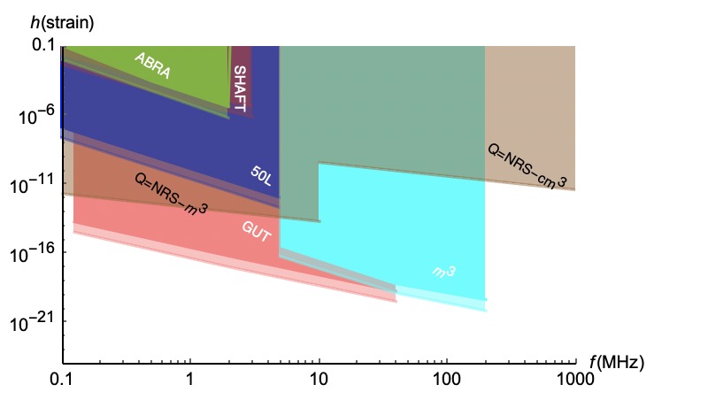
Figure 5: SNR=3 sensitivity for transient events, like PBH merger, and BH superradiance collapse. We use a bandwidth of $\Delta f=f$ for sensitivity estimate.

Mergers and superradiance collapses are two examples of potential nearly coherent sources, with short durations and certain directionality, which are viable sources for our detection scheme. We may also estimate the event rate around different sky angles, which we leave for future work.

Here we also comment on the sensitivity of the stochastic sources, and refer to Ref. Aggarwal et al. (2021) for detailed discussions. Many beyond the Standard Model scenarios in the early Universe can source stochastic gravitational waves, e.g. phase transition, preheating or reheating, and topological defects dynamics. Since gravitational waves play the same role as early universe radiation in the cosmic evolution, they are bounded by the effective number of additional neutrinos $\Delta N_{\text{eff}}$ as $h<10^{-27}(1\text{MHz}/f)\Delta N_{\text{eff}}^{1/2}$ Pisanti et al. (2021); Yeh et al. (2021). This means the amplitude of the stochastic gravitational wave is a few orders smaller than the coherent ones in general.

Especially, the signal from stochastic sources with random phases resembles white noise in one detector. One solution to identify such stochastic signals is through multiple detectors, in light of the pulsar timing array sensitivity of the stochastic gravitational waves. Considering our measurement scheme is electric in nature, two detectors moderately separated with cross-correlation of the electric signals may provide a certain signal-to-noise ratio of the stochastic background.

V Conclusion

To summarize, we consider a cryogenic detection scheme of the electric signals induced by gravitational waves via the inverse Gertsenshtein effect Gertsenshtein (1962), inside a strong static magnetic field. We make use of the transverse electric mode inside a quarterly-split cylinder geometry to maximize the signal induction from the oscillatory effective currents from gravitational waves. The current signal derives from the electric charge build-up on the surface of the cavity plates. We have performed EM simulation with the quarterly-split geometry and obtained the cavity’s form factor below the frequency of TE₂₁₁ mode, which characterizes the frequency response of our experimental setup. In the case of a narrow-frequency gravitational wave, the signal can be further enhanced by a large quality factor $Q$ that matches the bandwidth of the gravitational wave, and the corresponding strain sensitivity is projected to around $h\sim 10^{-20}\cdot(10^{6}/Q)$ for a meter-sized split cavity. For signals more extended in the frequency domain, we consider a broad-band signal with a characteristic frequency range wider than the cavity’s geometric bandwidth and make an estimate of our design’s sensitivity in broadband, non-resonant ($\Delta f\sim f$) mode. The broadband sensitivity is found to be $h\sim 10^{-13}$ for a meter-scale cavity.