High Tide or Riptide on the Cosmic Shoreline? A Water-Rich Atmosphere or Stellar Contamination for the Warm Super-Earth GJ 486b from JWST Observations

Abstract

Planets orbiting M-dwarf stars are prime targets in the search for rocky exoplanet atmospheres. The small size of M dwarfs renders their planets exceptional targets for transmission spectroscopy, facilitating atmospheric characterization. However, it remains unknown whether their host stars’ highly variable extreme-UV radiation environments allow atmospheres to persist. With JWST, we have begun to determine whether or not the most favorable rocky worlds orbiting M dwarfs have detectable atmospheres. Here, we present a 2.8–-5.2 $\micron$ JWST NIRSpec/G395H transmission spectrum of the warm (700 K, 40.3$\times$ Earth’s insolation) super-Earth GJ 486b (1.3 R_⊕ and 3.0 M_⊕). The measured spectrum from our two transits of GJ 486b deviates from a flat line at $2.2-3.3\sigma$, based on three independent reductions. Through a combination of forward and retrieval models, we determine that GJ 486b either has a water-rich atmosphere (with the most stringent constraint on the retrieved water abundance of H₂O $>$ 10% to 2$\sigma$) or the transmission spectrum is contaminated by water present in cool unocculted starspots. We also find that the measured stellar spectrum is best fit by a stellar model with cool starspots and hot faculae. While both retrieval scenarios provide equal quality fits ($\chi^{2}_{\nu}=1.0$) to our NIRSpec/G395H observations, shorter wavelength observations can break this degeneracy and reveal if GJ 486b sustains a water-rich atmosphere.

1 Introduction

Understanding the stability and longevity of atmospheres on rocky planets orbiting M dwarfs is paramount for understanding which, if any, of these planets may ultimately support life. However, given the high activity of most M-dwarf stars (e.g., Peacock et al., 2019), their planets are subject to extreme-UV radiation regimes that may remove any significant atmosphere through escape processes (e.g., Airapetian et al., 2020; Kasting & Pollack, 1983; Zahnle & Catling, 2017; Airapetian et al., 2017). This high activity also persists over much longer timescales given the long lifetimes of M dwarfs compared to larger stars (e.g., Loyd et al., 2021). M dwarfs also have the potential to impart spurious features into the transmission spectrum from inhomogenities in the stellar photosphere, a phenomenon called the “Transit Light Source effect” (TLS) (Rackham et al., 2018), also known as stellar contamination (Apai et al., 2018; Barclay et al., 2021; Garcia et al., 2022; Barclay et al., 2023).

Rocky worlds ($\leq$ 1.4R_⊕) are not predicted to retain hydrogen/helium-dominated atmospheres (Rogers, 2015; Rogers et al., 2021). This has been confirmed by observations of terrestrial planets, including the TRAPPIST-1 planets (de Wit et al., 2016, 2018; Wakeford et al., 2019; Garcia et al., 2022; Gressier et al., 2022), GJ 1132b (Diamond-Lowe et al., 2018; Mugnai et al., 2021; Libby-Roberts et al., 2022), the L98-59 system (Damiano et al., 2022; Zhou et al., 2023), LTT 1445Ab (Diamond-Lowe et al., 2022) and LHS 3488b (Kreidberg et al., 2019; Diamond-Lowe et al., 2020). However, many of these observations do not preclude higher mean molecular weight secondary atmospheres for these small planets (Moran et al., 2018; Damiano et al., 2022).

As part of the Cycle 1 JWST General Observer (GO) Program 1981 (PIs: K. Stevenson & J. Lustig-Yaeger), we are searching for atmospheric signatures on rocky planets around M dwarfs. Our program focuses reconnaissance on carbon dioxide (CO₂) and methane (CH₄), believed to produce the strongest signals in terrestrial atmospheres (Kaltenegger & Traub, 2009; Lustig-Yaeger et al., 2019). Both have strong bands between 3 and 5 $\mu$m, which can be probed by JWST. Secondary atmospheric CO₂ is also potentially common across a range of terrestrial planetary conditions via outgassing (Lincowski et al., 2018), as seen on Venus, Earth, and Mars. Using JWST, Program 1981 has already enabled a strong constraint on Earth-sized exoplanet LHS 475b, ruling out Earth-like, hydrogen/helium, water, or methane-dominated clear atmospheres Lustig-YaegerFu2023(Lustig-Yaeger & Fu et al. 2023).

Our ultimate aim is to trace the proposed cosmic shoreline, defined by Zahnle & Catling (2017). The cosmic shoreline describes the relationship between a planet’s escape velocity (${\rm v_{esc}}$) and insolation (${\rm I}$). This “shoreline” divides rocky bodies with atmospheres from those without and is shaped by various processes that cause atmospheric loss. In the solar system, this relationship follows ${\rm I\propto v{{}_{esc}}^{4}}$, suggesting that atmospheric escape mechanisms are dominated by thermal processes (Zahnle & Catling, 2017). Both thermal processes, such as Jeans escape and hydrodynamic escape, and non-thermal processes, encompassing photochemical escape and ion escape, cause composition-dependent atmospheric loss. These escape processes can be enhanced in planets around active stars through UV flaring or stellar winds. Thus, to understand any putative cosmic shoreline in the solar system or beyond, it is important to determine not only how planet size, mass, and atmospheric composition affect a planet’s ability to retain an atmosphere, but also the effect of the host star’s activity. These varying factors can reveal the mechanisms dominating atmospheric escape on a given world (e.g., Wordsworth & Kreidberg, 2022; McIntyre et al., 2023).

Here we present the results of our JWST-GO-1981 program observations for GJ 486b, a 1.3 R_⊕ and 3.0 M_⊕ planet (Caballero et al., 2022), with a zero Bond albedo equilibrium temperature of 700 K. GJ 486b has one of the highest transmission spectroscopy metrics (Kempton et al., 2018) of any known terrestrial exoplanet (Trifonov et al., 2021), making it a favorable target for study. The measured mass and radius indicate that GJ 486b is likely composed of a small metallic core, a deep silicate mantle, and a thin volatile upper layer (Caballero et al., 2022), which could be resistant to escape given the quiescent M3.5 V host star (0.339 R_⊙, T_eff = 3291 K; Caballero et al., 2022). Recent high-resolution observations of GJ 486b show that the planet does not possess a clear 1$\times$ solar atmosphere dominated by hydrogen/helium to high confidence ($\geq 5\sigma$). These observations also suggest that a clear, pure water atmosphere could be ruled out to low significance ($\leq 3\sigma$) (Ridden-Harper et al., 2022). We contextualize these observations in light of our own findings in Section 5.

2 JWST Observations of GJ 486b

We observed two transits of GJ 486b using the Near InfraRed Spectrograph (NIRSpec; Jakobsen et al., 2022; Birkmann et al., 2022) G395H instrument mode, covering wavelengths $2.87-5.14$ m at an average native spectral resolution $\mathcal{R}$ $\sim$ 2700.The G395H grating is split over two detectors, NRS1 and NRS2, with a gap from 3.72 to 3.82 $\mu$m. The first transit observation commenced on 25 December 2022 at 11:38 UTC and the second on 29 December 2022 at 21:15 UTC. Each observation lasted 3.53 hours, which covered the 1.01 hour transit duration and the required baseline. Both observations used the NIRSpec Bright Object Time Series (BOTS) mode with the NRSRAPID readout pattern, S1600A1 slit, and the SUB2048 subarray. For this bright target (K_mag = 6.4), we used 3 groups per integration and obtained 3507 integrations per exposure.

3 NIRSpec G395H Data Reduction

We reduced the data using three separate pipelines: Eureka! (Bell et al., 2022), FIREFLy (Rustamkulov et al., 2022, 2023), and Tiberius (Kirk et al., 2018, 2019, 2021). Each pipeline analysis is described below. Appendix A contains the updated system parameters obtained from each reduction. The three reductions showed a consistent offset in the measured transit depth for the Transit 1, NRS2 detector relative to the other three white light curve depths. We rule out astrophysical effects for this discrepancy and corrected it in each reduction as described in Appendix A.1.

3.1 Eureka!

We use a modified version of the jwst Stage 1 pipeline, starting from the _uncal.fits files. We perform group-level background subtraction before determining the flux per integration. For each group, we exclude the region within 9 pixels of the trace before computing and subtracting a median background value per pixel column. We process the _rateints.fits files through the regular jwst Stage 2 pipeline, skipping the flat fielding and absolute photometric calibration steps when our goal is to derive the planet’s spectrum at later stages. Conversely, we include these steps when our goal is to compute the flux-calibrated stellar spectrum (see Section 4.4). Stage 3 of Eureka! converts the time-series of 2D integrations into 1D spectra using optimal spectral extraction (Horne, 1986) and an aperture within 5 pixels of the trace. We flag bad pixels at numerous points within this stage using thresholds optimized to minimize scatter in the white light curves.

For the NRS1 detector, we extract the flux from 2.777 – 3.717 m and split the light into 47 spectroscopic light curves, each 20 nm (0.02 m) in width. For the NRS2 detector, we adopt the same resolution in extracting 67 spectroscopic light curves spanning 3.825 – 5.165 m. For each detector, we manually mask 9 pixel columns that exhibit significant scatter in their individual light curves. Doing so improves the quality of the spectroscopic light curves and yields more consistent transit depths.

With two NIRSpec detectors and two transit observations, we fit four white light curves and their systematics (see Figure 1). We determine the system parameters using batman (Kreidberg, 2015) and fix the quadratic limb-darkening coefficients to those provided by ExoTiC-LD (Grant & Wakeford, 2022), assuming the stellar parameters given by Trifonov et al. (2021) and the MPS-ATLAS set 1 models (Kostogryz et al., 2023). For the NRS1 detector, we find that a quadratic trend in time provides the best fit. For the NRS2 detector, a linear trend suffices to remove systematics. Table 1 lists our best-fit system parameters.

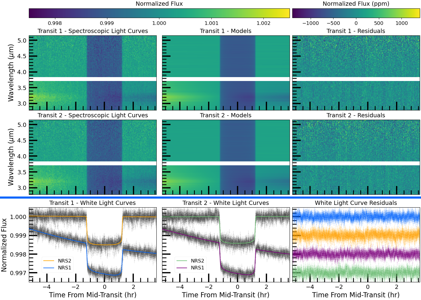
Figure 1: Eureka! spectroscopic and white light curves from two transits of GJ 486b. The top two rows contain the spectroscopic light curves (left), our best-fit models (center), and subsequent residuals (right) for each transit. Most evident in the data are wavelength-dependent ramps near 3.2 m that we readily remove. The bottom row depicts the white light curves from each detector (NRS1 and NRS2) before removing their systematic trends. Correlated noise is evident in the residuals and is likely due to thermal cycling (Rigby et al., 2022). The standard deviation of the normalized residuals is 140 ppm for NRS1 and 165 ppm for NRS2. The complete figure set (3 images, one for each reduction) is available in the online journal.

When fitting the spectroscopic light curves (see Figure 1), we fix the planet’s transit midpoint, inclination, and semi-major axis to the weighted mean values in Table 1. We fix the quadratic limb-darkening parameters to the values provided by ExoTiC-LD for each spectroscopic channel. For the NRS1 detector, we also fix the quadratic term in our time-dependent systematic model to that of the best-fit white light curve value (Transit 1: $c_{2}=0.0335$, Transit 2: $c_{2}=0.0248$). For all spectroscopic light curves, we fit for the zeroth and first-order terms ($c_{0}$ and $c_{1}$) of our polynomial. Light curves from the NRS2 detector only require a linear model in time. Including the term that rescales the uncertainties, each spectroscopic light curve has four free parameters, of which only the planet-to-star radius ratio is a physical parameter.

For each light curve, we first perform a least-squares minimization using the Powell method (Powell, 1964) and then initialize our MCMC routine using our best-fit values. We estimate the parameter uncertainties using emcee (Foreman-Mackey et al., 2013) and, at each iteration, we increase the uncertainties by an average factor of $\sim$1.5 to achieve a reduced $\chi^{2}=1$. All of our posteriors are Gaussian distributed and there are no parameter degeneracies.

3.2 FIREFLy

We run the jwst pipeline through Stages 1 and 2 using the uncal.fits files. We utilize group-level 1/f subtraction and apply a scaled superbias to account for the vertical offset seen in NRS2 Transit 1. (See Section A.1.) We correct for cosmic rays and bad and hot pixels in the Stage 2 output rateints.fits files and apply a second 1/f correction at the integration level by masking the spectral trace and then calculating the median of the background pixels in each column. This value is then subtracted from the cleaned 2D image.

We next cross-correlate each 2D image with the median aligned image to determine the x- and y-shifts of the spectral trace, which are used to align all 2D images. A Gaussian profile is then cross-correlated to each column in the y-direction and a fourth-order polynomial is fit in the x-direction to determine the spectral trace, which is used to extract the spectra.

The white light curves for Transits 1 and 2 are fit from the extracted spectra by summing the spectra in the wavelength direction over a detector. We fit $a/R_{\star}$, limb darkening parameters, and the impact parameter b using the weighted mean from both transits and both detectors. We then fix $a/R_{\star}$, b, and the period, and fit for $R_{P}/R_{\star}$, $T_{0}$, and limb darkening in the white light curve. A low-order polynomial in time (third-order in NRS1 and up to fourth-order for NRS2) was used to model the baseline, with additional detrending parameters of the x- and y-shifts and superbias scale factor. We then fix the system parameters (presented in Table 2) and limb-darkening coefficients in each wavelength column to fit the spectroscopic light curves.

3.3 Tiberius

With Tiberius we started by running STScI’s jwst stage 0 pipeline on the uncal.fits files from the group_scale step through gain_scale step. We set --odd_even_columns $=$ True at the ref_pix step and ran our own 1/f correction step at the group level prior to running ramp_fit, which removes the median background flux for every column of every group’s spectral image. We define the background as a 14-pixel-wide region that avoided 18 pixels centered on the curved trace, and mask bad pixels using our own custom bad pixel map. We subsequently ran assign_wcs and extract_2d to obtain the wavelength solution and proceeded to run Tiberius’s spectral extraction on the gainscalestep.fits files.

First we oversampled each pixel by a factor of 10 using a linear interpolation. This allows us to measure the stellar flux at the sub-pixel level, which reduces noise in the light curves (The JWST Transiting Exoplanet Community Early Release Science Team et al., 2022). We used a fourth order polynomial to trace the NRS1 detector stellar spectrum and a sixth order polynomial for NRS2. We performed standard aperture photometry at every pixel column, with a 4-pixel-wide aperture. We performed an additional background subtraction step at this stage by calculating the background in 14 pixels on either side of the trace, excluding 7 pixels on each side. For NRS1 we fit these background pixels with a linear polynomial while for NRS2 we used a median since our defined background regions were mostly above the stellar trace.

We remove cosmic rays and residual bad pixels manually and then correct for small shifts in the stellar spectra along the dispersion direction by cross-correlating all spectra in the time-series with the first, resampling each spectrum onto a common pixel grid. Finally, we created a white light curve between 2.75–3.72 $\mu$m for NRS1 and 3.83–5.15 $\mu$m for NRS2. Our spectroscopic light curves were created at 1 pixel resolution over the same wavelength range.

We fit the four white light curves (2 transits $\times$ 2 detectors) with batman (Kreidberg et al., 2015), leaving $a/R_{*}$, $R_{P}/R_{*}$, the orbital inclination ($i$), and the time of mid-transit ($T_{0}$) as free parameters, and fixing the period to the value from Trifonov et al. (2021). For our white and spectroscopic light curves, we assumed quadratic limb darkening with coefficients fixed to values from 3D stellar atmosphere models (Magic et al., 2015) using ExoTiC-LD (Grant & Wakeford, 2022). We adopted $T_{\mathrm{eff}}=3340$ K, [Fe/H] $=0.070$ and $\log g_{*}=4.9155$ (Trifonov et al., 2021). For our systematics model we used a combination of polynomials: quadratic-in-time, linear-in-x-position, and linear-in-y-position, resulting in 9 free parameters: 4 transit model parameters and 5 systematics model parameters.

To determine the best fitting values and uncertainties, we used emcee (Foreman-Mackey et al., 2013) with 90 walkers for two runs of 20,000 steps. After the first run we inflated our photometric uncertainties to give a reduced $\chi^{2}=1$ for our best-fitting model before the second run. Table 3 summarizes the results of our white light curve fits. For our spectroscopic light curve fits, we fixed $a/R_{*}$, $i$ and $T_{0}$ to the weighted mean values from our 4 white light curve fits and only fitted for $R_{P}/R_{*}$ and the 5 parameters defining our systematics model. Here we used a Levenberg-Marquadt sampler for computational speed as we had to fit 6876 spectroscopic light curves.

4 Interpretation of GJ 486b’s Transmission Spectrum

The three data reductions produce consistent spectra with a slight slope on the blue end ($\leq$ 3.7 $\mu$m) but are otherwise featureless. Here, we first quantify the significance of this slope in GJ 486b’s spectrum. We then proceed to offer physical explanations of the spectrum through forward modeling and retrieval analyses.

4.1 A Non-Flat Spectrum

We performed a flat line hypothesis rejection test to determine the statistical significance of the slope in the transmission spectrum. We fitted the spectrum from each pipeline using two models: a flat featureless model that uses one free parameter for the transit depth, and a Gaussian spectral feature model with four free parameters: the flat transit depth and the central wavelength, amplitude, and width of a Gaussian feature added to the baseline featureless spectrum. We fitted both models to each dataset using the dynesty nested sampling code for Bayesian inference (Speagle, 2020) and then used the Bayesian evidence to calculate the Bayes factor of each model (e.g., Trotta, 2008, 2017). We then converted the Bayes factors to more classical “sigma” detection significances using the relationship detailed by Benneke & Seager (2013).

Figure 2 demonstrates that each spectrum separately favors the Gaussian model and rejects a featureless spectrum. The strength of the signal detection is $3.20\sigma$ for Eureka!, $2.24\sigma$ for FIREFLy, and $3.29\sigma$ for Tiberius. The FIREFLy detection significance is lower due to slightly larger uncertainties associated with that reduction, which stem from FIREFLy’s choice of spectroscopic binning to produce similar transit depth errors across the full wavelength range and wavelength-dependent baseline functions. Nevertheless, the same shape is seen in the spectra from the three pipelines. Thus, the flat line hypothesis is rejected by all three analyses with varying confidence. Each individual reduction hypothesis rejection test is available in the online journal.

Figure 2: Relative transmission spectra of the three data reductions (Eureka!: blue circles, FIREFLy: orange squares, Tiberius: green triangles). The median fit to the Eureka! dataset using an agnostic Gaussian model is shown in purple bounded by $1\sigma$ and $3\sigma$ Bayesian credibility envelopes. The legend displays the statistical significance with which each reduction rules out a flat line in favor of the Gaussian model. Analyses of all three reductions reveal an uptick at the blue end of the wavelength range. Instrument throughput deteriorates in the grey shaded region and the measured transit depths become unreliable; thus we exclude points within this region from our hypothesis rejection tests.

4.2 Forward Modeling Tentatively Supports an Atmosphere with Water Vapor

We ran a suite of forward models using the stellar and planet parameters from Caballero et al. (2022) to compare to each transmission spectrum. We also generated forward models using an updated stellar log(g) = $4.91\pm 0.02$, obtained from our updated $a/R_{s}$ constraints (See Appendix A) (Seager & Mallén-Ornelas, 2003; Sandford & Kipping, 2017), finding consistent results.

We focus on higher mean molecular weight scenarios to explain the transmission spectrum. For completeness, however, we simulate a 1000$\times$ solar metallicity atmosphere with a parameterized pressure-temperature profile in thermochemical equilibrium with CHIMERA (Line & Yung, 2013; Line et al., 2014) as in our previous work (Lustig-Yaeger et al., 2023). We include the species H2O, CH4, CO, CO2, NH3, HCN, H2S, H2, and He. The CHIMERA thermochemical equilibrium abundances result in a model spectrum that is primarily shaped by methane, carbon dioxide, and water. After generating the temperature-pressure profile and atmospheric abundances with CHIMERA, we use the radiative transfer suite of PICASO (Batalha et al., 2019), with opacities resampled to $R=10,000$ from Batalha et al. (2020), to generate model spectra.

In each case, we bin the resulting model transmission spectrum to the resolution of the data before performing a reduced-$\chi^{2}$ comparison. The full datasets of all three reductions to which we fit our forward models and retrievals can be found with the Supplemental Materials. As with the Gaussian hypothesis tests, we exclude the data points in the grey shaded region of Figure 2 from our model-fitting due to steeply-falling instrument throughput at these wavelengths ($<$ 2.87).

As shown in Figure 3, the slight slope and flatness of the spectra from each reduction allow us to confidently disregard low mean molecular weight atmospheres dominated by hydrogen/helium – up to metallicities of 1000$\times$ solar – to greater than 3$\sigma$. This improves upon the previous high resolution data obtained by Ridden-Harper et al. (2022) that could only strongly rule out atmospheres up to a few times solar. Our 1000$\times$ solar metallicity atmosphere has an average mean molecular weight of 13.86 g/mol compared to the high resolution’s 5 g/mol limit, though our constraint is less stringent for non-chemically consistent atmospheres (see Section 4.3).

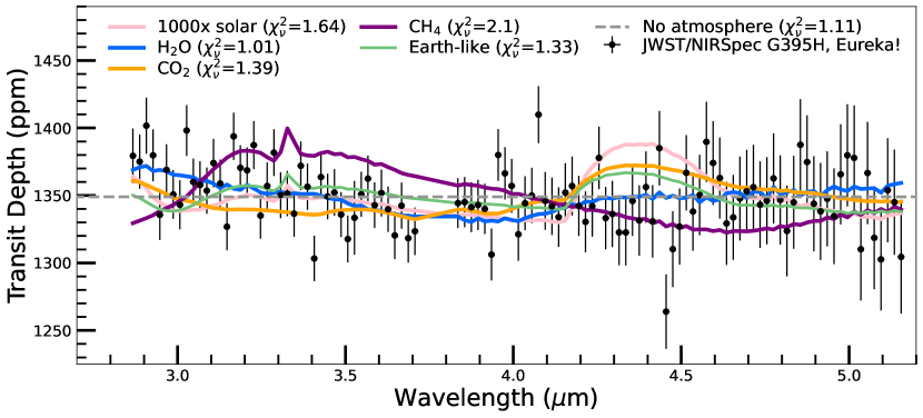
Figure 3: Our final Eureka! spectra of GJ 486b binned to R$\sim$200 (black points) compared to a set of PICASO forward models (colored lines: 1000$\times$ solar, pink; H₂O, blue; CO₂, orange; CH₄, purple; Earth-composition, green). A 1 bar, pure water atmosphere on GJ 486b fits the data with the lowest reduced-$\chi^{2}$ (1.01), and a flat-line model (dashed grey line) is nearly as well fit by the data (reduced-$\chi^{2}$ = 1.11), though is weakly rejected by Gaussian vs flat line tests. Alternatively, stellar contamination with water in the atmosphere of the star, rather than the planet, can explain the observed transit depths (see Fig. 4).

We also compare the data from each reduction to a set of end-member forward models from PICASO with single-gas 1 bar, isothermal atmospheres. For ease of interpretation, we focus here on the results from the Eureka! reduction, as we determined that it was the most representative dataset, with the smallest weighted average deviation from the median of all three reductions. However, the trend in best-fit agrees among all three reductions (for a complete description of each reduction’s fit, see Table 4 in Appendix B). The slight slope on the blue end of NRS1 results in best-fitting (reduced-$\chi^{2}$ = 1.01) forward models that contain pure water vapor, as this molecule has a strong absorption feature from 2.2 to 3.7 $\mu$m, consistent with the slope we observe in NRS1.

Our data across all reductions also moderately to weakly rule out carbon-rich atmospheres of either CH₄ or CO₂ to 6.5$\sigma$ and 2.3$\sigma$, respectively. A flat-line model, representative of an airless body or a high-altitude (0.1 $\mu$bar) cloud deck, fit the data with reduced-$\chi^{2}$ = 1.11, which is statistically equivalent to the clear water atmosphere model within the forward modeling framework. However, between its equilibrium temperature and size, GJ 486b is not expected to support clouds to such low pressures, as there are few condensible species in this temperature range. Photochemical hazes could dampen the presence of any spectral features with a haze layer at this altitude and create a flat line spectrum (Gao et al., 2020; Pidhorodetska et al., 2021; Caballero et al., 2022); however, given the Bayesian evidence of the Gaussian absorption tests discussed above, the water atmosphere is the preferred explanation from the PICASO analysis for all reductions. We note that the FIREFLy reduction only weakly rejects the flat line hypothesis and, therefore, an airless planet or very hazy planet is still a possibility. In Figure 3, we show the results of our PICASO forward modeling compared to the Eureka! data. The full set of results for each reduction is available in the online journal.

4.3 Retrievals Suggest a Water-rich Atmosphere or Unocculted Starspot Contamination

In addition to our forward model comparisons, we performed an atmospheric retrieval analysis to assess the robustness of our tentative evidence for a water-rich atmosphere and consider alternative astrophysical explanations. We apply two independent retrieval codes — POSEIDON (MacDonald & Madhusudhan, 2017; MacDonald, 2023) and rfast (Robinson & Salvador, 2023) — to all three data reductions to ensure reliable inferences.

4.3.1 Water-rich Atmosphere Scenario

Our POSEIDON atmospheric retrieval considers six potential gases that can range in abundance from being trace volatiles to the dominant background gas: N₂, H₂, H₂O, CH₄, CO₂, and CO. The opacity contributions from these gases include line opacity (Polyansky et al., 2018; Yurchenko et al., 2017; Tashkun & Perevalov, 2011; Li et al., 2015) and collision-induced absorption (CIA) from H₂-H₂, H₂-N₂, H₂-CH₄, H₂-CO₂, CO₂-CO₂, CO₂-CH₄, and N₂-N₂ (Karman et al., 2019). Since the mixing ratios must sum to unity, we have five free parameters describing their mixing ratios that each follow centered log-ratio (CLR) priors, ranging from $10^{-12}$ to 1, as described by Lustig-YaegerFu2023Lustig-Yaeger & Fu et al. (2023). The other free parameters are the isothermal temperature ($\mathcal{U}$ [200 K, 900 K]), the atmosphere radius at the 1 bar reference pressure ($\mathcal{U}$ [0.9 $R_{\rm{p,\,obs}}$, 1.1 $R_{\rm{p,\,obs}}$]), and the log-pressure of an opaque surface ($\mathcal{U}$ [-7, 2], in bar). We calculate transmission spectra via opacity sampling at a resolving power of $R=$ 20,000 from 0.5–5.4 $\micron$, with the lower wavelength limit set far below our shortest wavelength (2.8 $\micron$) to later demonstrate how retrieval solutions diverge at optical wavelengths. These 8-parameter POSEIDON retrievals used the PyMultiNest (Feroz et al., 2009; Buchner et al., 2014) package to explore the parameter space with 2,000 live points.

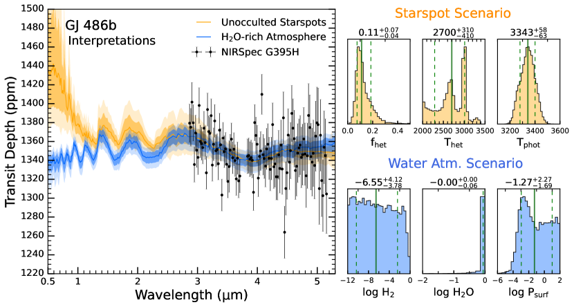
Figure 4: POSEIDON retrieval results for GJ 486b’s transmission spectrum. Left: retrieved transmission spectra for two models compared to the JWST NIRSpec G395H data from the Eureka! reduction (black points with error bars). Two scenarios can equivalently explain GJ 486b’s transmission spectrum ($\chi^{2}_{\nu}=1.0$): unocculted starspots with no planetary atmosphere (orange contours) or a water-rich atmosphere with no starspots (blue contours). The median retrieved spectrum (solid lines) and 1$\sigma$ and 2$\sigma$ confidence intervals (dark and light contours) for each scenario are overlaid. Top right: posterior histograms for the unocculted starspot model, defined by the fractional coverage area of cold stellar heterogeneities/spots (f_het), the temperature of the heterogeneities/spots (T_het), and the stellar photospheric temperature (T_phot). Bottom right: posterior histogram for the water-rich atmosphere scenario, highlighting hydrogen and water’s retrieved mixing ratios alongside the atmospheric surface pressure. Water is necessary to explain GJ 486b’s spectrum, but the retrievals cannot differentiate between a water-rich planetary atmosphere or water contained in cool starspots that contaminate the transmission spectrum. The complete figure set (3 images, one for each reduction) is available in the online journal.

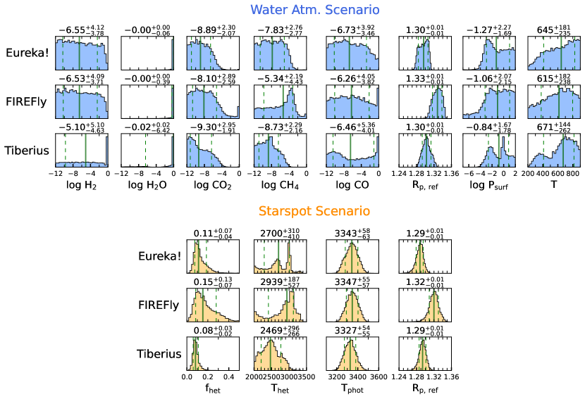
Figure 6: Posterior probability distributions from the POSEIDON retrievals. Top rows (blue): retrieval model where GJ 486b’s spectrum is caused by a water-rich atmosphere. Bottom rows (orange): retrieval model instead considering unocculted starspots. The rows in each scenario correspond to different data reductions (Eureka!, FIREFLy, and Tiberius from top to bottom).

Figure 4 shows our POSEIDON retrieval results for this atmospheric model scenario (blue retrieved spectrum and histograms) for the Eureka! data reduction – see the online figure set for the other two reductions. For Eureka! and FIREFLy, the preferred explanation for the observed rise in the blue wavelengths of the transmission spectrum is H₂O opacity from the wing of the band centered on 2.8 m. Bayesian model comparisons favor the presence of H₂O with Bayes factors of 133 and 8 (3.6$\sigma$ and 2.6$\sigma$) for Eureka! and FIREFLy, respectively. The retrieved H₂O abundance posterior indicates that water is the most likely background gas (e.g., Eureka! requires a H₂O mixing ratio $>$ 10% to 2$\sigma$ confidence), with an upper limit ruling out a H₂-dominated atmosphere. The Eureka! and Tiberius reductions also yield upper limits on the CH₄ and CO₂ abundances (see the Appendix, Figure 6). The Tiberius reduction, however, does not uniquely infer a water-rich atmosphere. Though a water-rich atmosphere remains the preferred solution for Tiberius, a secondary mode permits a clear, H₂-dominated atmosphere with no other gases contributing to the spectrum. This secondary mode reflects a solution where the wavelength dependence of H₂-H₂ CIA is used to fit the spectrum. This solution is unphysical since an H₂-dominated atmosphere will always contain other trace molecules with more prominent absorption features at these wavelengths. Upon further investigation, we found that the unphysical solution is driven by the upwards rise at the longest wavelengths that are only present in the Tiberius reduction (see Figure 2). We, therefore, conclude that a consistent explanation for GJ 486b’s transmission spectrum, assuming the observed non-flatness is caused by atmospheric absorption, can be readily explained ($\chi^{2}_{\nu}\approx 1.0$) by a water-rich atmosphere — in agreement with the forward models in Section 4.2.

We also conducted single-composition atmospheric retrievals with rfast for all three reductions. These retrievals consider atmospheres with a single absorbing gas alongside a spectrally inactive background gas with an agnostic mean molecular weight. Our rfast retrieval model has 6 free parameters: the log-gas mixing ratio, $\log_{10}f_{\mathrm{gas}}$ ($\mathcal{U}$ [-12, 0]), the log-surface pressure, $\log_{10}P_{0}$ ($\mathcal{U}$ [-1, 6], in Pa), the surface temperature, $T_{0}$ ($\mathcal{U}$ [300, 1100] K), the mean molecular weight of the background gas, $m_{b}$ ($\mathcal{U}$ [2, 50] amu), the planet radius, $R_{p}$ ($\mathcal{U}$ [1.1, 1.4] $R_{\oplus}$), and the planet mass, $M_{p}$ ($\mathcal{N}$ [2.28, 0.12] $M_{\oplus}$). For the single gases, we consider, in separate retrievals, H₂O, CO₂, CO, and CH₄. The rfast retrievals use emcee (Foreman-Mackey et al., 2013) with 100 walkers for 15,000 steps, where the first 5,000 are discarded for burn-in.

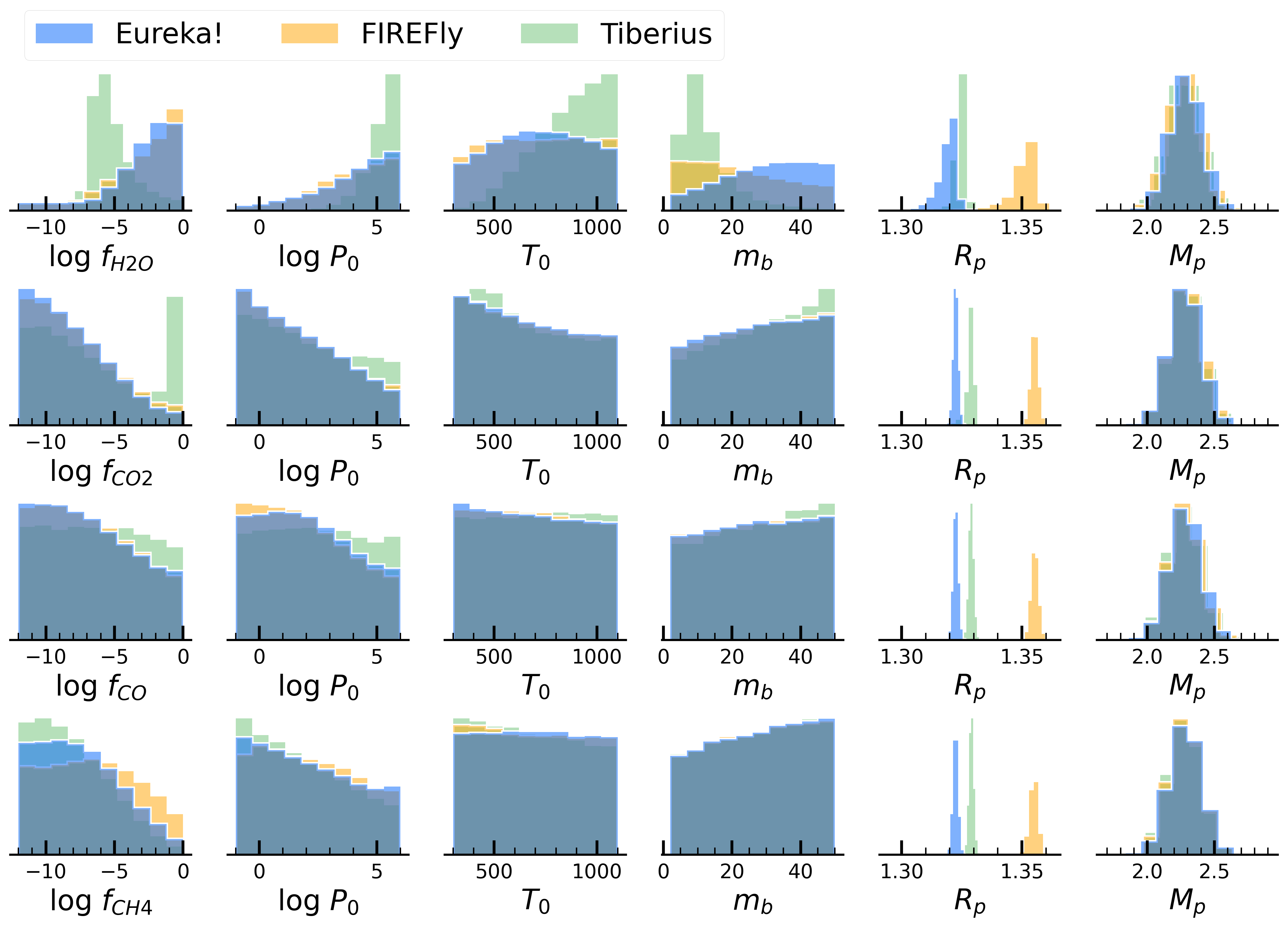
Figure 7: The 1D posteriors for rfast single-gas retrievals. From top to bottom water, carbon dioxide, carbon monoxide, and methane. Each reduction is shown in its own color with Eureka! in blue, FIREFLy in orange and Tiberius in green.

We show our rfast 1D posteriors in the Appendix (Figure 7). Our rfast retrievals also identify a H₂O-rich atmosphere as a consistent explanation for the Eureka! and FIREFLy reductions (though the lower limits on H₂O are weaker compared with POSEIDON due to the combination of a free mean molecular weight, planet mass, and log-uniform vs. CLR priors). rfast also finds that the Tiberius reduction permits lower mean-molecular weight atmospheres for similar reasons to POSEIDON.

4.3.2 Unocculted Starspot Scenario

We now consider the potential for GJ 486b’s host star alone to explain our observed transmission spectrum. Stellar heterogeneities (starspots and/or faculae) that are not occulted during transit can induce wavelength-dependent features in transmission spectra if the stellar intensity illuminating the planetary atmosphere differs from the overall average stellar intensity — also known as the transit light source effect (TLS) (e.g., Rackham et al., 2018). This confounding stellar influence is a crucial consideration for transmission spectra of planets orbiting cool M dwarfs, such as GJ 486, since H₂O existing in cold starspots could mimic atmospheric signatures.

We implement stellar contamination retrievals with POSEIDON following a similar approach to Rathcke et al. (2021), based on the parameterization from Pinhas et al. (2018). The contamination model is defined by four parameters: the stellar heterogeneity temperature, $T_{\rm{het}}$ ($\mathcal{U}$ [2300 K, 1.2 $T_{*,\rm{eff}}$]), the heterogeneity coverage fraction, $f_{\rm{het}}$ ($\mathcal{U}$ [0, 0.5]), the stellar photosphere temperature, $T_{\rm{phot}}$ ($\mathcal{N}$ [$T_{*,\rm{eff}}$, $\sigma_{T_{*,\rm{eff}}}$]), and the planetary radius, $R_{p}$ ($\mathcal{U}$ [0.9 $R_{\rm{p,\,obs}}$, 1.1 $R_{\rm{p,\,obs}}$]). For the priors, we adopt literature values of $T_{*,\rm{eff}}=3340$ K and $\sigma_{T_{*,\rm{eff}}}=54$ K (Trifonov et al., 2021). We calculate the stellar contamination factor by interpolating the Allard et al. (2012) grid of stellar PHOENIX models using the pysynphot package (STScI Development Team, 2013).

Figure 4 demonstrates that contamination from unocculted starspots, with no planetary atmosphere, provides an equally plausible ($\chi^{2}_{\nu}\approx 1.0$) alternative explanation to GJ 486b’s transmission spectrum. In this scenario, the observed slope in the spectrum is still caused by the wing of an H₂O band, but the water resides in the host star. The POSEIDON retrievals for all three data reductions yield a spot coverage fraction of $\sim 10\%$, but with relatively weak and inconsistent constraints on the spot temperature. Compared to a flat spectrum, the unocculted starspot model is preferred with Bayes factors of 255, 16, and 114 (3.8$\sigma$, 2.9$\sigma$, and 3.5$\sigma$) for Eureka!, FIREFLy, and Tiberius, respectively. We stress that, while our present observations cannot distinguish between the water-rich atmosphere scenario and unocculted starspots, these two scenarios deviate substantially at shorter wavelengths (see Figure 4). Consequently, even in the case of aerosol-laden atmospheres (Rackham et al., 2022), future observations at shorter wavelengths can readily distinguish which scenario is correct.

4.4 A Spotty Star Best Explains the Stellar Spectrum

To further investigate the possibility of stellar contamination, we return to the JWST/NIRSpec G395H data to probe the Stage 3 stellar spectra and examine whether the star is consistent with a particular stellar model. Upon completing Stage 2 of the jwst pipeline with the flat fielding and absolute photometric calibration steps enabled, we noticed that only the region within 8 pixels of the trace is converted to units of MJy. The remaining pixel regions are in DN/s, so we manually mask them before running Stage 3 of Eureka!. Due to the lack of unmasked background pixels, we disable Stage 3 background subtraction for this flux-calibrated reduction. This change does not skew the final calibrated spectrum since we already performed group-level background subtraction in Stage 1.

To compute the stellar baseline spectrum, we exclude 1040 integrations during transit (1560 - 2599) and then compute median values along the time axis. We manually mask a few obvious outliers before estimating the baseline spectrum uncertainties by computing the standard deviation in flux along the time axis. Typical uncertainties are 3 – 5 mJy, but can be as large as 55 mJy for some spectral channels. The typical uncertainty values are consistent with the uncertainties derived from our standard spectral extraction routine. We do not use the standard error calculation for our uncertainties. That is, we do not divide our uncertainties by the square root of the number of integrations because, as demonstrated below, the standard deviation in flux better represents the true uncertainty in our flux-calibrated spectrum. We note that the derived baseline spectrum is remarkably consistent between both transits (see Figure 5).

We used PHOENIX stellar models produced by Allard et al. (2012) to analyze whether the observed stellar baseline spectrum is best explained by a spotless or spotted star. We utilized the Allard et al. (2012) models, as in Section 4.3.2, because they account for the formation of molecular bands including H₂O, CH₄, and TiO₂ and have higher ($\Delta\lambda$=2 Å) resolution than the observations. This grid of models also has sufficient temperature and gravity coverage to model the photospheres of M-dwarf stars and their spots and faculae ($T_{\rm eff}$ $\geq$ 2000 K, log($g$) = 0 – 6 cm s^-2).

We employed single PHOENIX models to represent spotless (or one-component) stars. We used weighted linear combinations of PHOENIX models to create inhomogeneous models. Two-component models include one model with $T_{\rm eff}$ $\geq$ 3000 K to represent the background photosphere and a second, cooler model with $T_{\rm eff}$ $\leq$ $T_{\rm eff,photosphere}$ - 100 K to represent spots. Three-component models include an additional $T_{\rm eff}$ $\geq$ $T_{\rm eff,photosphere}$ + 100 K model to represent faculae. In the two- and three-component models, all spots have the same $T_{\rm eff}$ and log($g$), as do the faculae. Linear combinations were computed by interpolating the spot and faculae models onto the photosphere wavelength grid before summing the fluxes in a weighted fraction where the photosphere was required to be $\geq$ 50% of the total.

To compare the models to the observed baseline spectra, we converted the native wavelengths from Å to $\mu$m and the flux densities from ergs s^-1 cm^-2 cm^-1 to fluxes in units of mJy. We then scaled the models by R${}_{*}^{2}$/dist² using literature values for GJ 486: R_∗=0.33 R_⊙ (Trifonov et al., 2021) and dist = 8.07 pc (Gaia Collaboration et al., 2021). We smoothed and interpolated the models to be the same resolution as the observations before calculating a reduced-$\chi^{2}$. In our reduced-$\chi^{2}$ calculations, we considered 3187 wavelength points for Transit 1 (3180 for Transit 2) and three fitted parameters ($T_{\rm eff}$, log($g$), and a scaling factor). The multi-component models included additional fit parameters for determining the percent coverage for the spots and faculae. The scaling factor was multiplied by the R${}_{*}^{2}$/dist² term to account for uncertainty in either measured quantity and varied from 0.9 to 1.1. To get the final reduced-$\chi^{2}$ value for each model, we computed reduced-$\chi^{2}$ individually for Transits 1 and 2 and then took the average.

Figure 5: Best matching one-, two-, and three-component PHOENIX models to the Baseline GJ 486 spectra from Transits 1 (green) and 2 (black). The bottom two panels zoom-in on the grey highlighted regions of the top panel spectrum. When considering a one-component photosphere, a $T_{\rm{eff}}$ = 3300 K, log($g$)=4.5 cgs model is preferred (purple, $\chi^{2}_{\nu}$ = 72.0). When allowing for spots in a two-component model, a warmer $T_{\rm{eff}}$ = 3400 K, log($g$)=5 cgs photosphere with 25% coverage of $T_{\rm{eff}}$ = 3000 K, log($g$)=5 cgs spots is the preferred model (blue, $\chi{{}^{2}}_{\nu}$ = 53.4). The best overall match to the observations is produced with a three-component photosphere+spots+faculae model that has a background photosphere with $T_{\rm{eff}}$ = 3200 K, log($g$)=5 cgs, 20% spot coverage ($T_{\rm{eff}}$ = 3000 K, log($g$)=5 cgs), and 25% faculae coverage ($T_{\rm{eff}}$ = 3400 K, log($g$)=5 cgs) (orange, $\chi^{2}_{\nu}$ = 49.0).

Considering each type of one-, two-, and three-component model individually, we find that the models with the smallest reduced-$\chi^{2}$ values are fairly consistent with the existing literature values, though no model is a particularly good fit with a reduced-$\chi^{2}$ near 1 (for numerical details, see Appendix C). A 100% $T_{\rm eff}$ = 3300 K, log($g$)=4.5 cgs model with $\chi_{\nu}^{2}$=72.0 is the preferred one-component photosphere model (scale factor = 1.05), yielding a lower surface gravity than expected for a field age mid-M-dwarf like GJ 486. In agreement with our updated log($g$)=4.91$\pm$0.02 cgs, we disfavor the low stellar surface gravity of the best-matched photosphere-only model when taking into account inhomogeneities on the stellar surface. A 75% $T_{\rm eff}$ = 3400 K, log($g$)=5 cgs background photosphere with 25% spot coverage at $T_{\rm eff}$ = 3000 K, log($g$)=5 cgs is the preferred two-component model ($\chi_{\nu}^{2}$=53.4; scale factor = 1.05). The model most preferred overall is a three-component model with $\chi_{\nu}^{2}$=49.0 that has a background photosphere with $T_{\rm eff}$ = 3200 K, log($g$)=5 cgs, 20% spot coverage at $T_{\rm eff}$ = 3000 K, log($g$)=5 cgs, and 25% faculae coverage at $T_{\rm eff}$ = 3400 K, log($g$)=5 cgs (scale factor = 1.1). These three models are shown in Figure 5 compared to the Baseline GJ 486 spectra from Transits 1 and 2. There is decent general agreement for each model throughout the full $\sim$2.9-5 $\mu$m range, with slightly better agreement for the three-component photosphere+spot+faculae model, indicating that we cannot rule out star spots as a source for the presumed water detection.

5 Discussion and Conclusions

There is remarkable agreement in the stellar heterogeneity parameters obtained from a) retrieving for unocculted star spots in the planetary transmission spectrum and b) fitting the baseline stellar spectrum with PHOENIX multi-component stellar models. Both lines of inquiry find best fits with overlapping values for faculae/spot coverage and temperature as well as the photospheric temperature. The stellar spectrum is best fit by a 3200 K photosphere with 20% cool spots at 3000 K and 25% hot faculae at 3400 K. These values match well compared to the TLS retrievals with a 3280 K photospheric temperature lower limit and cool spots up to $\sim$3100K at 7 - 18% coverage (see Figure 6). This consistency lends strong support to this physical interpretation of our JWST NIRSpec/G395H data. Moreover, even quiescent M dwarfs are known to be highly hetereogenous with strong impacts on the transmission spectrum (Rackham et al., 2018; Zhang et al., 2018; Somers et al., 2020).

Our forward model water atmosphere demonstrates that water is the best-fit absorber to explain GJ 486b’s spectrum in the absence of stellar contamination. Such a pure steam atmosphere could theoretically be generated by impacts from small, icy bodies (Zahnle et al., 1988) or outgassed depending on the mantle composition (Tian & Heng, 2023), but would be quickly lost via the runaway greenhouse effect (Goldblatt et al., 2013), as well as being disfavored by high resolution observations (Ridden-Harper et al., 2022). We examine the effect of adding CO₂ to our H₂O forward model, finding that scaling the carbon content upwards always results in a worse fit to the data. In the water-rich POSEIDON retrievals, we find strong water abundance lower limits across the three reductions, with an agnostic background gas prior. Two carbon species have stringent upper limits: carbon dioxide and methane. All reductions have posteriors where the constrained carbon species abundances can supersede that of water, but the best fits prefer atmospheres where water vapor dominates over carbon species. Such atmospheres would be challenging to maintain at GJ 486b’s 700 K equilibrium temperature, given our current understanding of the runaway greenhouse effect (Goldblatt et al., 2013) and expected limits on the interior sequestration and outgassing rates of carbon species relative to water (Sossi et al., 2023; Tian & Heng, 2023). However, given the large range of retrieved abundances compatible with GJ 486’s spectrum, they remain consistent with atmospheric theory. Furthermore, our retrievals cannot constrain the abundance of carbon monoxide (CO), providing an additional potential reservoir for carbon in the atmosphere. A warm, water-rich atmosphere with little atmospheric carbon would represent a terrestrial exoplanet wholly unlike any solar system analogue and challenge our understanding of atmospheric formation (Wordsworth & Kreidberg, 2022; McIntyre et al., 2023).

GJ 486b joins the ranks of other terrestrial M-dwarf planets with tantalizing atmospheric inferences. Such planets include the first planet of our JWST-GO-1981 program, LHS 475b, exisiting observations of which cannot distinguish a carbon dioxide atmosphere from an airless body (Lustig-Yaeger et al., 2023). L 98-59c is another planet where recent HST observations have tentatively suggested either a hydrogen-rich planetary atmosphere or stellar contamination (Barclay et al., 2023) — though a different analysis favored a flat, featureless transmission spectrum (Zhou et al., 2023). Both GJ 486b at 1.3 R_⊕ and L 98-59c at 1.35 R_⊕ track the upper edge of planets below the expected hydrogen-dominated atmospheric cut-off (Rogers, 2015; Rogers et al., 2021). Their difference in insolation, with GJ 486b at T_eq = 700 K and L 98-59c at T_eq = 550 K, combined with their retrieved upper limit atmospheric hydrogen fractions, offer suggestive hints at a cosmic shoreline that is confounded by potential stellar contamination. More data are clearly necessary to confidently mark the boundaries of any cosmic shoreline.

Secondary eclipse observations of GJ 486b with JWST’s Mid-Infrared Instrument (MIRI) Low Resolution Spectroscopy (LRS) mode are already scheduled (GO 1743, PI: Mansfield). These observations will measure the dayside emission spectrum of the planet, allowing an expected $5\sigma$ constraint on surface pressures $\geq 1$ bar, as well as providing evidence for the atmospheric composition with a sufficiently thick atmosphere (Mansfield et al., 2019, 2021). Thus, these MIRI/LRS observations can lend an additional line of evidence for or against both a significant atmosphere as well as the presence of water. However, our water-rich atmospheric retrieval scenario demonstrates that much lower surface pressures (down to millibar levels) are consistent with the data from NIRSpec/G395H, which is beyond the sensitivity of the planned MIRI/LRS observations. In this case, the secondary eclipse emission spectrum is unlikely to provide strong evidence in favor of either of our interpretations for GJ 486b.

As seen in Figure 4, the unocculted star spot scenario and the water-rich atmosphere scenario diverge strongly shortwards of 0.8 $\mu$m. In the case that the upcoming MIRI observations cannot definitely detect an atmosphere, high precision shorter wavelength observations could provide evidence for or against an atmosphere on GJ 486b. Ultimately, our JWST NIRSpec/G395H stellar and transmission spectra, combined with retrievals and stellar models, suggest either an airless planet with a spotted host star or a significant planetary atmosphere containing water vapor. Given the agreement between our stellar modeling and atmospheric retrievals for the spot scenario, this interpretation may have a slight edge over a water-rich atmosphere. However, a true determination of the nature of GJ 486b remains on the horizon, with wider wavelength observations holding the key to this world’s location along the cosmic shoreline.

Appendix A Data Reduction

Dataset	$T_{0}$ (BJDTDB)	$i$ (∘)	$a/Rs_{*}$	$R_{P}/R_{*}$	Residual RMS (ppm)
Transit 1, NRS1	$2459939.071619^{+2.0e-05}_{-2.1e-05}$	$89.10^{+0.26}_{-0.35}$	$11.24^{+0.03}_{-0.09}$	$0.03697\pm 0.00009$	143
Transit 1, NRS2	$2459939.071570^{+2.4e-05}_{-2.4e-05}$	$89.06^{+0.34}_{-0.38}$	$11.22^{+0.06}_{-0.13}$	$0.03784\pm 0.00009$	171
Transit 2, NRS1	$2459943.472959^{+2.0e-05}_{-2.0e-05}$	$89.02^{+0.35}_{-0.38}$	$11.23^{+0.07}_{-0.13}$	$0.03689\pm 0.00009$	137
Transit 2, NRS2	$2459943.472974^{+2.3e-05}_{-2.4e-05}$	$89.06^{+0.46}_{-0.47}$	$11.22^{+0.10}_{-0.19}$	$0.03670\pm 0.00009$	158
Weighted Mean	$2459939.071594\pm 1.6e-05$	$89.06\pm 0.18$	$11.229\pm 0.043$	$0.03709\pm 0.00004$	n/a
	$2459943.472967\pm 1.5e-05$

Table 1: Best-fit system parameters and 1$\sigma$ uncertainties from fitting the four white light curves using Eureka!.

Dataset	$T_{0}$ (BJDTDB)	$i$ (∘)	$a/Rs_{*}$	$R_{P}/R_{*}$	Residual RMS (ppm)
Transit 1, NRS1	2459939.0716102 $\pm$ 2.1e-05	89.11 $\pm$ 0.35	11.294 $\pm$ 0.137	0.03759 $\pm$ 0.00013	132
Transit 1, NRS2	2459939.0715592 $\pm$ 2.2e-05	89.97 $\pm$ 0.27	11.449 $\pm$ 0.023	0.03791 $\pm$ 0.00010	159
Transit 2, NRS1	2459943.4729689 $\pm$ 1.9e-05	89.99 $\pm$ 0.22	11.446 $\pm$ 0.021	0.03784 $\pm$ 0.00013	130
Transit 2, NRS2	2459943.4730019 $\pm$ 2.3e-05	89.30 $\pm$ 0.40	11.325 $\pm$ 0.111	0.03742 $\pm$ 0.00017	158
Weighted Mean	2459939.0715859 $\pm$1.5e-05	89.75 $\pm$ 0.14	11.443 $\pm$ 0.015	0.03775 $\pm$ 0.000063	n/a
	2459943.4729823 $\pm$ 1.5e-05

Table 2: The system parameters resulting from the FIREFLy fits to the white light curves.

Dataset	$T_{0}$ (BJDTDB)	$i$ (∘)	$a/Rs_{*}$	$R_{P}/R_{*}$	Residual RMS (ppm)
Transit 1, NRS1	$2459939.071586^{+3.5e-05}_{-3.6e-05}$	$89.99^{+0.65}_{-0.61}$	$11.34^{+0.04}_{-0.13}$	$0.03683\pm 0.00015$	158
Transit 1, NRS2	$2459939.071548^{+3.6e-05}_{-3.5e-05}$	$89.97^{+0.67}_{-0.62}$	$11.36^{+0.05}_{-0.13}$	$0.03756\pm 0.00017$	188
Transit 2, NRS1	$2459943.472952^{+3.6e-05}_{-3.5e-05}$	$90.02^{+0.75}_{-0.72}$	$11.42^{+0.06}_{-0.17}$	$0.03684\pm 0.00015$	158
Transit 2, NRS2	$2459943.472955^{+4.3e-05}_{-4.3e-05}$	$89.83^{+1.35}_{-1.32}$	$11.23^{+0.19}_{-0.4}$	$0.03685\pm 0.00019$	194
Weighted Mean	$2459939.07158\pm 1.9e-05$	$89.96\pm 0.37$	$11.40\pm 0.06$	$0.03701\pm 8e-05$	n/a

Table 3: The system parameters resulting from the Tiberius fits to the white light curves.

A.1 Data Reduction Consistency: An Offset between the NRS1 and NRS2 Detectors

As stated in the main text, all initial reductions showed a consistent offset in measured transit depth for the Transit 1, NRS2 detector relative to the other white light curve depths. Since this shift is not seen in the NRS1 detector, we can confidently rule out all astrophysical effects (e.g., stellar variability) as a source of the discrepancy. For the FIREFLy reduction, we altered our application of the superbias in the bias subtraction step and light-curve fitting stages, which we found produced more consistent transit depths for NRS1 and NRS2.

In our FIREFLy reduction, we measured the superbias level by rescaling the superbias image to match the level in the trace-masked groups of each integration. We note that a full readout of the detector mitigates bias drifts using reference pixels, but the subarray readouts used here do not have such pixels. We find that the superbias level changes by hundreds of ppm throughout the time series, with typical values of the scaling factor about 1.003. We use the standard-deviation-normalized time series of the superbias scaling coefficient as a detrending vector at the light-curve fitting stage, added linearly to our usual systematics model. We find that the superbias decorrelation coefficient is statistically preferred in the systematics model, with some residual structure in the photometry well-explained by this term. The addition of superbias detrending reduced the transit depth tension between NRS1 and NRS2, with the white-light curve transit depths agreeing within the uncertainties.

For the Eureka! reduction, we also investigated time-dependent variations in the NRS2 detector bias level. We found that applying a scale factor correction to the superbias frame for each integration in Stage 1 marginally improved the consistency in measured transit depths (by $\sim 20$ ppm), but also led to increased scatter. Applying a single scale factor correction for all integrations yielded a similar improvement, but without the increased scatter. We continue to investigate different methods of scaling the superbias frame. In the meantime, we elect to adopt the standard bias correction in our final Eureka! analysis and apply a manual offset of 78 ppm in transit depth to NRS2, Transit 1.

To account for NRS2 transit visit discrepancy for the final Tiberius reduction, we also manually offset the transmission spectrum for NRS2, Transit 1 by 63 ppm, such that the median transit depth was equal to NRS2, Transit 2.

After this superbias-detrending in FIREFLy and manual offsets in Eureka! and Tiberius, we saw excellent agreement between the Eureka!, FIREFLy, and Tiberius spectra across both NRS1 and NRS2 in both transits, as shown in Figure 2. Since the superbias correction alters FIREFLy’s absolute transit depths, we elect to compare their relative transit depths.

Appendix B Interpretation Supplemental Information

CHIMERA	Eureka!	FIREFLy	Tiberius	Average $\sigma$	Significance
Forward Model	(dof = 110)	(dof = 46)	(dof = 46)	ruled out
1000$\times$ solar	1.64	1.26	2.44	3.6	moderately ruled out
H2O, 1 bar	1.01	0.76	1.37	0.9	consistent with data
CO2, 1 bar	1.39	1.17	1.63	2.3	weakly/moderately ruled out
CH4, 1 bar	2.10	1.77	5.96	6.5	strongly ruled out
Earth-like	1.33	1.04	2.35	2.8	moderately ruled out
Flat line	1.11	0.91	1.60	1.5	weakly/moderately rejected by Gaussian fitting

Table 4: Each reduction’s reduced-$\chi^{2}$ compared to our end-member composition PICASO forward models. Since each reduction has a different degree-of-freedom (dof), we also report the average significance (in $\sigma$, following Trotta (2017)) by which the model is ruled out. Note that the “flat line” model can correspond either to an airless planet or a very hazy atmosphere.

Appendix C Stellar Model Statistics

Model Configuration	$\chi_{\nu}^{2}$	$\chi^{2}$	$n$	$K$
Photosphere	72.0	228,680.81	3,187	3
Photosphere+Spot	53.4	169,489.64	3,187	5
Photosphere+Spot+Faculae	49.0	155,374.94	3,187	7

Table 5: Summary of values for our goodness-of-fit testing, where $n$ is the number of wavelength points, and $K$ is the number of free parameters.

References

- Airapetian et al. (2017) Airapetian, V. S., Glocer, A., Khazanov, G. V., et al. 2017, ApJ, 836, L3, doi: 10.3847/2041-8213/836/1/L3
- Airapetian et al. (2020) Airapetian, V. S., Barnes, R., Cohen, O., et al. 2020, International Journal of Astrobiology, 19, 136, doi: 10.1017/S1473550419000132
- Allard et al. (2012) Allard, F., Homeier, D., & Freytag, B. 2012, Philosophical Transactions of the Royal Society of London Series A, 370, 2765, doi: 10.1098/rsta.2011.0269
- Apai et al. (2018) Apai, D., Rackham, B. V., Giampapa, M. S., et al. 2018, arXiv e-prints, arXiv:1803.08708, doi: 10.48550/arXiv.1803.08708
- Astropy Collaboration et al. (2013) Astropy Collaboration, Robitaille, T. P., Tollerud, E. J., et al. 2013, A&A, 558, A33, doi: 10.1051/0004-6361/201322068
- Astropy Collaboration et al. (2018) Astropy Collaboration, Price-Whelan, A. M., Sipőcz, B. M., et al. 2018, AJ, 156, 123, doi: 10.3847/1538-3881/aabc4f
- Barclay et al. (2021) Barclay, T., Kostov, V. B., Colón, K. D., et al. 2021, AJ, 162, 300, doi: 10.3847/1538-3881/ac2824
- Barclay et al. (2023) Barclay, T., Sheppard, K. B., Latouf, N., et al. 2023, arXiv e-prints, arXiv:2301.10866, doi: 10.48550/arXiv.2301.10866
- Batalha et al. (2020) Batalha, N., Freedman, R., Lupu, R., & Marley, M. 2020, Resampled Opacity Database for PICASO v2, 1.0, Zenodo, doi: 10.5281/zenodo.3759675
- Batalha et al. (2019) Batalha, N. E., Lewis, T., Fortney, J. J., et al. 2019, ApJ, 885, L25, doi: 10.3847/2041-8213/ab4909
- Bell et al. (2022) Bell, T. J., Ahrer, E.-M., Brande, J., et al. 2022, arXiv e-prints, arXiv:2207.03585. https://arxiv.org/abs/2207.03585
- Benneke & Seager (2013) Benneke, B., & Seager, S. 2013, ApJ, 778, 153, doi: 10.1088/0004-637X/778/2/153
- Birkmann et al. (2022) Birkmann, S. M., Ferruit, P., Giardino, G., et al. 2022, A&A, 661, A83, doi: 10.1051/0004-6361/202142592
- Bourque et al. (2021) Bourque, M., Espinoza, N., Filippazzo, J., et al. 2021, The Exoplanet Characterization Toolkit (ExoCTK), 1.0.0, Zenodo, doi: 10.5281/zenodo.4556063
- Buchner et al. (2014) Buchner, J., Georgakakis, A., Nandra, K., et al. 2014, A&A, 564, A125, doi: 10.1051/0004-6361/201322971
- Bushouse et al. (2022) Bushouse, H., Eisenhamer, J., Dencheva, N., et al. 2022, JWST Calibration Pipeline, 1.8.2, Zenodo, doi: 10.5281/zenodo.7325378
- Caballero et al. (2022) Caballero, J. A., González-Álvarez, E., Brady, M., et al. 2022, A&A, 665, A120, doi: 10.1051/0004-6361/202243548
- Chen & Kipping (2017) Chen, J., & Kipping, D. 2017, ApJ, 834, 17, doi: 10.3847/1538-4357/834/1/17
- Damiano et al. (2022) Damiano, M., Hu, R., Barclay, T., et al. 2022, AJ, 164, 225, doi: 10.3847/1538-3881/ac9472
- de Wit et al. (2016) de Wit, J., Wakeford, H. R., Gillon, M., et al. 2016, Nature, 537, 69, doi: 10.1038/nature18641
- de Wit et al. (2018) de Wit, J., Wakeford, H. R., Lewis, N. K., et al. 2018, Nature Astronomy, 2, 214, doi: 10.1038/s41550-017-0374-z
- Diamond-Lowe et al. (2018) Diamond-Lowe, H., Berta-Thompson, Z., Charbonneau, D., & Kempton, E. M. R. 2018, AJ, 156, 42, doi: 10.3847/1538-3881/aac6dd
- Diamond-Lowe et al. (2020) Diamond-Lowe, H., Charbonneau, D., Malik, M., Kempton, E. M. R., & Beletsky, Y. 2020, AJ, 160, 188, doi: 10.3847/1538-3881/abaf4f
- Diamond-Lowe et al. (2022) Diamond-Lowe, H., Mendonça, J. M., Charbonneau, D., & Buchhave, L. A. 2022, arXiv e-prints, arXiv:2210.11809, doi: 10.48550/arXiv.2210.11809
- Feroz et al. (2009) Feroz, F., Hobson, M. P., & Bridges, M. 2009, MNRAS, 398, 1601, doi: 10.1111/j.1365-2966.2009.14548.x
- Foreman-Mackey et al. (2013) Foreman-Mackey, D., Hogg, D. W., Lang, D., & Goodman, J. 2013, PASP, 125, 306, doi: 10.1086/670067
- Gaia Collaboration et al. (2021) Gaia Collaboration, Brown, A. G. A., Vallenari, A., et al. 2021, A&A, 649, A1, doi: 10.1051/0004-6361/202039657
- Gao et al. (2020) Gao, P., Thorngren, D. P., Lee, E. K. H., et al. 2020, Nature Astronomy, 4, 951, doi: 10.1038/s41550-020-1114-3
- Garcia et al. (2022) Garcia, L. J., Moran, S. E., Rackham, B. V., et al. 2022, A&A, 665, A19, doi: 10.1051/0004-6361/202142603
- Goldblatt et al. (2013) Goldblatt, C., Robinson, T. D., Zahnle, K. J., & Crisp, D. 2013, Nature Geoscience, 6, 661, doi: 10.1038/ngeo1892
- Grant & Wakeford (2022) Grant, D., & Wakeford, H. R. 2022, Exo-TiC/ExoTiC-LD: ExoTiC-LD v3.0.0, v3.0.0, Zenodo, doi: 10.5281/zenodo.7437681
- Gressier et al. (2022) Gressier, A., Mori, M., Changeat, Q., et al. 2022, A&A, 658, A133, doi: 10.1051/0004-6361/202142140
- Harris et al. (2020) Harris, C. R., Millman, K. J., van der Walt, S. J., et al. 2020, Nature, 585, 357, doi: 10.1038/s41586-020-2649-2
- Horne (1986) Horne, K. 1986, Publ. Astron. Soc. Pac., 98, 609, doi: 10.1086/131801
- Hunter (2007) Hunter, J. D. 2007, Computing in Science Engineering, 9, 90, doi: 10.1109/MCSE.2007.55
- Jakobsen et al. (2022) Jakobsen, P., Ferruit, P., Alves de Oliveira, C., et al. 2022, A&A, 661, A80, doi: 10.1051/0004-6361/202142663
- Kaltenegger & Traub (2009) Kaltenegger, L., & Traub, W. A. 2009, ApJ, 698, 519, doi: 10.1088/0004-637X/698/1/519
- Karman et al. (2019) Karman, T., Gordon, I. E., van der Avoird, A., et al. 2019, Icarus, 328, 160, doi: 10.1016/j.icarus.2019.02.034
- Kasting & Pollack (1983) Kasting, J. F., & Pollack, J. B. 1983, Icarus, 53, 479, doi: 10.1016/0019-1035(83)90212-9
- Kempton et al. (2018) Kempton, E. M. R., Bean, J. L., Louie, D. R., et al. 2018, PASP, 130, 114401, doi: 10.1088/1538-3873/aadf6f
- Kirk et al. (2019) Kirk, J., López-Morales, M., Wheatley, P. J., et al. 2019, AJ, 158, 144, doi: 10.3847/1538-3881/ab397d
- Kirk et al. (2018) Kirk, J., Wheatley, P. J., Louden, T., et al. 2018, MNRAS, 474, 876, doi: 10.1093/mnras/stx2826
- Kirk et al. (2021) Kirk, J., Rackham, B. V., MacDonald, R. J., et al. 2021, AJ, 162, 34, doi: 10.3847/1538-3881/abfcd2
- Kostogryz et al. (2023) Kostogryz, N., Shapiro, A. I., Witzke, V., et al. 2023, Research Notes of the American Astronomical Society, 7, 39, doi: 10.3847/2515-5172/acc180
- Kreidberg (2015) Kreidberg, L. 2015, PASP, 127, 1161, doi: 10.1086/683602
- Kreidberg et al. (2015) Kreidberg, L., Line, M. R., Bean, J. L., et al. 2015, ApJ, 814, 66, doi: 10.1088/0004-637X/814/1/66
- Kreidberg et al. (2019) Kreidberg, L., Koll, D. D. B., Morley, C., et al. 2019, Nature, 573, 87, doi: 10.1038/s41586-019-1497-4
- Li et al. (2015) Li, G., Gordon, I. E., Rothman, L. S., et al. 2015, The Astrophysical Journal Supplement Series, 216, 15, doi: 10.1088/0067-0049/216/1/15
- Libby-Roberts et al. (2022) Libby-Roberts, J. E., Berta-Thompson, Z. K., Diamond-Lowe, H., et al. 2022, AJ, 164, 59, doi: 10.3847/1538-3881/ac75de
- Lincowski et al. (2018) Lincowski, A. P., Meadows, V. S., Crisp, D., et al. 2018, ApJ, 867, 76, doi: 10.3847/1538-4357/aae36a
- Line et al. (2014) Line, M. R., Knutson, H., Wolf, A. S., & Yung, Y. L. 2014, ApJ, 783, 70, doi: 10.1088/0004-637X/783/2/70
- Line & Yung (2013) Line, M. R., & Yung, Y. L. 2013, ApJ, 779, 3, doi: 10.1088/0004-637X/779/1/3
- Loyd et al. (2021) Loyd, R. O. P., Shkolnik, E. L., Schneider, A. C., et al. 2021, ApJ, 907, 91, doi: 10.3847/1538-4357/abd0f0
- Lustig-Yaeger et al. (2019) Lustig-Yaeger, J., Meadows, V. S., & Lincowski, A. P. 2019, ApJ, 887, L11, doi: 10.3847/2041-8213/ab5965
- Lustig-Yaeger et al. (2023) Lustig-Yaeger, J., Fu, G., May, E. M., et al. 2023, arXiv e-prints, arXiv:2301.04191, doi: 10.48550/arXiv.2301.04191
- MacDonald (2023) MacDonald, R. J. 2023, The Journal of Open Source Software, 8, 4873, doi: 10.21105/joss.04873
- MacDonald & Madhusudhan (2017) MacDonald, R. J., & Madhusudhan, N. 2017, MNRAS, 469, 1979, doi: 10.1093/mnras/stx804
- Magic et al. (2015) Magic, Z., Chiavassa, A., Collet, R., & Asplund, M. 2015, Astronomy & Astrophysics, 573, A90
- Mansfield et al. (2021) Mansfield, M., Bean, J. L., Kempton, E. M. R., et al. 2021, Constraining the Atmosphere of the Terrestrial Exoplanet Gl486b, JWST Proposal. Cycle 1, ID. #1743
- Mansfield et al. (2019) Mansfield, M., Kite, E. S., Hu, R., et al. 2019, ApJ, 886, 141, doi: 10.3847/1538-4357/ab4c90
- McIntyre et al. (2023) McIntyre, S. R. N., King, P. L., & Mills, F. P. 2023, MNRAS, 519, 6210, doi: 10.1093/mnras/stad095
- Moran et al. (2018) Moran, S. E., Hörst, S. M., Batalha, N. E., Lewis, N. K., & Wakeford, H. R. 2018, AJ, 156, 252, doi: 10.3847/1538-3881/aae83a
- Mugnai et al. (2021) Mugnai, L. V., Modirrousta-Galian, D., Edwards, B., et al. 2021, AJ, 161, 284, doi: 10.3847/1538-3881/abf3c3
- Peacock et al. (2019) Peacock, S., Barman, T., Shkolnik, E. L., Hauschildt, P. H., & Baron, E. 2019, ApJ, 871, 235, doi: 10.3847/1538-4357/aaf891
- Pérez & Granger (2007) Pérez, F., & Granger, B. E. 2007, Computing in Science and Engineering, 9, 21, doi: 10.1109/MCSE.2007.53
- Pidhorodetska et al. (2021) Pidhorodetska, D., Moran, S. E., Schwieterman, E. W., et al. 2021, AJ, 162, 169, doi: 10.3847/1538-3881/ac1171
- Pinhas et al. (2018) Pinhas, A., Rackham, B. V., Madhusudhan, N., & Apai, D. 2018, MNRAS, 480, 5314, doi: 10.1093/mnras/sty2209
- Polyansky et al. (2018) Polyansky, O. L., Kyuberis, A. A., Zobov, N. F., et al. 2018, MNRAS, 480, 2597, doi: 10.1093/mnras/sty1877
- Powell (1964) Powell, M. J. D. 1964, The Computer Journal, 7, 155, doi: 10.1093/comjnl/7.2.155
- Rackham et al. (2018) Rackham, B. V., Apai, D., & Giampapa, M. S. 2018, ApJ, 853, 122, doi: 10.3847/1538-4357/aaa08c
- Rackham et al. (2022) Rackham, B. V., Espinoza, N., Berdyugina, S. V., et al. 2022, arXiv e-prints, arXiv:2201.09905, doi: 10.48550/arXiv.2201.09905
- Rathcke et al. (2021) Rathcke, A. D., MacDonald, R. J., Barstow, J. K., et al. 2021, AJ, 162, 138, doi: 10.3847/1538-3881/ac0e99
- Ridden-Harper et al. (2022) Ridden-Harper, A., Nugroho, S., Flagg, L., et al. 2022, arXiv e-prints, arXiv:2212.11816, doi: 10.48550/arXiv.2212.11816
- Rigby et al. (2022) Rigby, J., Perrin, M., McElwain, M., et al. 2022, arXiv e-prints, arXiv:2207.05632. https://arxiv.org/abs/2207.05632
- Robinson & Salvador (2023) Robinson, T. D., & Salvador, A. 2023, \psj, 4, 10, doi: 10.3847/PSJ/acac9a
- Rogers et al. (2021) Rogers, J. G., Gupta, A., Owen, J. E., & Schlichting, H. E. 2021, MNRAS, 508, 5886, doi: 10.1093/mnras/stab2897
- Rogers (2015) Rogers, L. A. 2015, ApJ, 801, 41, doi: 10.1088/0004-637X/801/1/41
- Rustamkulov et al. (2022) Rustamkulov, Z., Sing, D. K., Liu, R., & Wang, A. 2022, ApJ, 928, L7, doi: 10.3847/2041-8213/ac5b6f
- Rustamkulov et al. (2023) Rustamkulov, Z., Sing, D. K., Mukherjee, S., et al. 2023, Nature, 614, 659, doi: 10.1038/s41586-022-05677-y
- Salvatier et al. (2016) Salvatier, J., Wieckiâ, T. V., & Fonnesbeck, C. 2016, PyMC3: Python probabilistic programming framework, Astrophysics Source Code Library, record ascl:1610.016. http://ascl.net/1610.016
- Sandford & Kipping (2017) Sandford, E., & Kipping, D. 2017, AJ, 154, 228, doi: 10.3847/1538-3881/aa94bf
- Seager & Mallén-Ornelas (2003) Seager, S., & Mallén-Ornelas, G. 2003, ApJ, 585, 1038, doi: 10.1086/346105
- Somers et al. (2020) Somers, G., Cao, L., & Pinsonneault, M. H. 2020, ApJ, 891, 29, doi: 10.3847/1538-4357/ab722e
- Sossi et al. (2023) Sossi, P. A., Tollan, P. M. E., Badro, J., & Bower, D. J. 2023, Earth and Planetary Science Letters, 601, 117894, doi: 10.1016/j.epsl.2022.117894
- Speagle (2020) Speagle, J. S. 2020, MNRAS, 493, 3132, doi: 10.1093/mnras/staa278
- STScI Development Team (2013) STScI Development Team. 2013, pysynphot: Synthetic photometry software package, Astrophysics Source Code Library, record ascl:1303.023. http://ascl.net/1303.023
- Tashkun & Perevalov (2011) Tashkun, S. A., & Perevalov, V. I. 2011, Journal of Quantitative Spectroscopy and Radiative Transfer, 112, 1403, doi: 10.1016/j.jqsrt.2011.03.005
- The JWST Transiting Exoplanet Community Early Release Science Team et al. (2022) The JWST Transiting Exoplanet Community Early Release Science Team, Ahrer, E.-M., Alderson, L., et al. 2022, arXiv e-prints, arXiv:2208.11692. https://arxiv.org/abs/2208.11692
- Tian & Heng (2023) Tian, M., & Heng, K. 2023, arXiv e-prints, arXiv:2301.10217, doi: 10.48550/arXiv.2301.10217
- Trifonov et al. (2021) Trifonov, T., Caballero, J. A., Morales, J. C., et al. 2021, Science, 371, 1038, doi: 10.1126/science.abd7645
- Trotta (2008) Trotta, R. 2008, Contemporary Physics, 49, 71, doi: 10.1080/00107510802066753
- Trotta (2017) —. 2017, arXiv e-prints, arXiv:1701.01467, doi: 10.48550/arXiv.1701.01467
- van der Walt et al. (2011) van der Walt, S., Colbert, S. C., & Varoquaux, G. 2011, Computing in Science Engineering, 13, 22, doi: 10.1109/MCSE.2011.37
- Virtanen et al. (2020) Virtanen, P., Gommers, R., Oliphant, T. E., et al. 2020, Nature Methods, 17, 261, doi: https://doi.org/10.1038/s41592-019-0686-2
- Wakeford et al. (2019) Wakeford, H. R., Lewis, N. K., Fowler, J., et al. 2019, AJ, 157, 11, doi: 10.3847/1538-3881/aaf04d
- Wordsworth & Kreidberg (2022) Wordsworth, R., & Kreidberg, L. 2022, ARA&A, 60, 159, doi: 10.1146/annurev-astro-052920-125632
- Yurchenko et al. (2017) Yurchenko, S. N., Amundsen, D. S., Tennyson, J., & Waldmann, I. P. 2017, Astronomy and Astrophysics, 605, A95, doi: 10.1051/0004-6361/201731026
- Zahnle & Catling (2017) Zahnle, K. J., & Catling, D. C. 2017, The Astrophysical Journal, 843, 122, doi: 10.3847/1538-4357/aa7846
- Zahnle et al. (1988) Zahnle, K. J., Kasting, J. F., & Pollack, J. B. 1988, Icarus, 74, 62, doi: 10.1016/0019-1035(88)90031-0
- Zhang et al. (2018) Zhang, Z., Zhou, Y., Rackham, B. V., & Apai, D. 2018, AJ, 156, 178, doi: 10.3847/1538-3881/aade4f
- Zhou et al. (2023) Zhou, L., Ma, B., Wang, Y.-H., & Zhu, Y.-N. 2023, Research in Astronomy and Astrophysics, 23, 025011, doi: 10.1088/1674-4527/acaceb