Molecular Design Based on Integer Programming and Splitting Data Sets by Hyperplanes

Jianshen Zhu¹, Naveed Ahmed Azam^2,∗, Kazuya Haraguchi¹, Liang Zhao³, Hiroshi Nagamochi¹ and Tatsuya Akutsu⁴

¹ Department of Applied Mathematics and Physics, Kyoto University, Kyoto 606-8501, Japan
² Department of Mathematics, Quaid-i-Azam University, Islamabad 45320, Pakistan
³ Graduate School of Advanced Integrated Studies in Human Survavibility (Shishu-Kan), Kyoto University, Kyoto 606-8306, Japan
⁴ Bioinformatics Center, Institute for Chemical Research, Kyoto University, Uji 611-0011, Japan
^∗ Corresponding author

Abstract
A novel framework for designing the molecular structure of chemical compounds with a desired chemical property has recently been proposed. The framework infers a desired chemical graph by solving a mixed integer linear program (MILP) that simulates the computation process of a feature function defined by a two-layered model on chemical graphs and a prediction function constructed by a machine learning method. To improve the learning performance of prediction functions in the framework, we design a method that splits a given data set $\mathcal{C}$ into two subsets $\mathcal{C}^{(i)},i=1,2$ by a hyperplane in a chemical space so that most compounds in the first (resp., second) subset have observed values lower (resp., higher) than a threshold $\theta$. We construct a prediction function $\psi$ to the data set $\mathcal{C}$ by combining prediction functions $\psi_{i},i=1,2$ each of which is constructed on $\mathcal{C}^{(i)}$ independently. The results of our computational experiments suggest that the proposed method improved the learning performance for several chemical properties to which a good prediction function has been difficult to construct.

Keywords: Machine Learning, Integer Programming, Chemo-informatics, Materials Informatics, QSAR/QSPR, Molecular Design.

1 Introduction

Background  Among various application areas of bioinformatics and machine learning, drug design is gathering interest [1, 2]. Accordingly, extensive studies have been done on computational analysis of chemical structures. There are two major topics in such studies: prediction of the chemical property of a given chemical structure, and design of a chemical structure having a desired chemical property. These topics have also been extensively studied in the field of chemoinformatics, where the former one is referred to as quantitative structure activity relationship (QSAR) [3] and the latter as inverse quantitative structure activity relationship (inverse QSAR) [4, 5, 6].

For the prediction task, statistical methods and machine learning methods have been extensively utilized [3]. In most of such studies, there are two phases: learning phase and prediction phase. In the learning phase, a prediction function is derived from training data consisting of pairs of chemical structures and their activities (or properties), where each chemical structure is given as an undirected graph (called a chemical graph) and then is transformed into a vector of real numbers called features or descriptors. In the prediction phase, the prediction function derived as above is simply applied to the feature vector obtained from a given chemical graph. To derive a prediction function, regression-based methods have been utilized in traditional QSAR studies [3], where machine learning-based methods, including artificial neural network (ANN)-based methods [7, 8], have recently been extensively utilized. It is to be noted that when using graph convolutional networks (GCNs) [9], chemical graphs can be directly handled and thus transformation to feature vectors is not necessarily required.

For the design task, prediction functions are also utilized and are usually derived from existing data as in the above. Then, chemical structures are inferred from given chemical activities through a prediction function [4, 5, 6] where additional constraints may be imposed to restrict the possible structures. In the traditional approach, this inference task consists of two phases, (i) derivation of feature vectors from given chemical activities using the inverse of the prediction function, and (ii) reconstruction of chemical structures from given feature vectors, where these two phases are often mixed. For (i), some optimization methods and/or sampling methods are usually employed. For (ii), some enumeration methods are often applied. However, both are inverse problems and are computationally difficult. For example, it is known that the number of possible chemical graphs is huge [10] and inference of a chemical graph from a given feature vector is NP-hard in general [11]. Therefore, most existing methods employ heuristic methods for both (i) and (ii), and thus do not guarantee optimal or exact solutions.

Recently, different approaches have been proposed for the design task using ANNs. One of the attractive points of ANNs is that generative models are available, which include autoencoders and generative adversarial networks. Furthermore, as mentioned before, chemical structures can be directly handled by using GCNs [9]. By combining these techniques, it might be possible to design novel chemical structures without solving the inverse problems [12]. Indeed, extensive studies have recently been done using various ANN models, which include variational autoencoders [13], grammar variational autoencoders [14], generative adversarial networks [15], recurrent neural networks [16, 17], and invertible flow models [18, 19]. However, these are heuristic methods (although based on some statistical models) and thus do not guarantee optimality or exactness of the solutions.

Figure 1: An illustration of inferring desired chemical graphs $\mathbb{C}\in\mathcal{G}_{\sigma}$ with $\underline{y^{*}}\leq\eta(f(\mathbb{C}))\leq\overline{y^{*}}$.

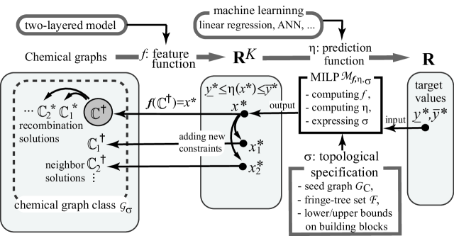
Framework  A novel framework for inferring chemical graphs has been developed [20, 21, 22, 23] based on an idea of formulating as a mixed integer linear programming (MILP), the computation process of a prediction function constructed by a machine learning method. The unique point of this framework is that once a prediction function is formulated, the inverse problem can be solved exactly by applying an MILP solver. It consists of two main phases: the first phase constructs a prediction function $\eta$ for a chemical property and the second phase infers a chemical graph with a target value of the property based on the function $\eta$. For a chemical property $\pi$, let $\mathcal{C}_{\pi}$ be a data set of chemical graphs such that the observed value $a(\mathbb{C})$ of property $\pi$ for every chemical graph $\mathbb{C}\in\mathcal{C}_{\pi}$ is available. In the first phase, we introduce a feature function $f:\mathcal{G}\to\mathbb{R}^{K}$ for a positive integer $K$, where the descriptors of a chemical graph are defined based on local graph structures in a special way called a two-layered model. We then construct a prediction function $\eta$ by a machine learning method such as linear regression, decision tree and an ANN so that the output $y=\eta(x)\in\mathbb{R}$ of the feature vector $x=f(\mathbb{C})\in\mathbb{R}^{K}$ for each $\mathbb{C}\in\mathcal{C}_{\pi}$ serves as a predicted value to the real value $a(\mathbb{C})$. In the second phase of inferring a desired chemical graph, we specify not only a target chemical value for property $\pi$ but also an abstract structure for a chemical graph to be inferred. The latter is described by a set of rules based on the two-layered model called a topological specification $\sigma$, and denote by $\mathcal{G}_{\sigma}$ the set of all chemical graphs that satisfy the rules in $\sigma$. The users select topological specification $\sigma$ and two reals $\underline{y}^{*}$ and $\overline{y}^{*}$ as an interval for a target chemical value. The task of the second phase is to infer chemical graphs $\mathbb{C}^{*}\in\mathcal{G}_{\sigma}$ such that $\underline{y}^{*}\leq\eta(f(\mathbb{C}^{*}))\leq\overline{y}^{*}$ (see Figure 1 for an illustration). For this, we formulate an MILP $\mathcal{M}_{f,\eta,\sigma}$ that represents (i) the computation process of $x:=f(\mathbb{C})$ from a chemical graph $\mathbb{C}$ in the feature function $f$; (ii) the computation process of $y:=\eta(x)$ from a vector $x\in\mathbb{R}^{K}$ in the prediction function $\eta$; and (iii) the constraint for $\mathbb{C}\in\mathcal{G}_{\sigma}$. Given an interval with $\underline{y}^{*},\overline{y}^{*}\in\mathbb{R}$, we solve the MILP $\mathcal{M}_{f,\eta,\sigma}$ to find a feature vector $x^{*}\in\mathbb{R}^{K}$ and a chemical graph $\mathbb{C}^{\dagger}\in\mathcal{G}_{\sigma}$ such that $f(\mathbb{C}^{\dagger})=x^{*}$ and $\underline{y}^{*}\leq\eta(x^{*})\leq\overline{y}^{*}$ (where if the MILP instance is infeasible then this suggests that $\mathcal{G}_{\sigma}$ does not contain such a desired chemical graph). In the second phase, we next generate some other desired chemical graphs based on the solution $\mathbb{C}^{\dagger}$. For this, the following two methods have been designed.

The first method constructs isomers of $\mathbb{C}^{\dagger}$ without solving any new MILP. In this method, we first decompose the chemical graph $\mathbb{C}^{\dagger}$ into a set of chemical acyclic graphs $T^{\dagger}_{1},T^{\dagger}_{2},\ldots,T^{\dagger}_{q}$, and next construct a set $\mathcal{T}_{i}$ of isomers $T^{*}_{i}$ of each tree $T^{\dagger}_{i}$ such that $f(T^{*}_{i})=f(T^{\dagger}_{i})$ by a dynamic programming algorithm due to Azam et al. [24]. Finally we choose an isomer $T^{*}_{i}\in\mathcal{T}_{i}$ for each $i=1,2,\ldots,q$ and assemble them into an isomer $\mathbb{C}^{*}\in\mathcal{G}_{\sigma}$ of $\mathbb{C}^{\dagger}$ such that $f(\mathbb{C}^{*})=x^{*}=f(\mathbb{C}^{\dagger})$. The first method generates such isomers $\mathbb{C}_{1}^{*},\mathbb{C}_{2}^{*},\ldots$ which we call recombination solutions of $\mathbb{C}^{\dagger}$.

The second method constructs new solutions by solving the MILP $\mathcal{M}_{f,\eta,\sigma}$ with an additional set $\Theta$ of new linear constraints [23]. We first prepare arbitrary $p_{\mathrm{dim}}$ linear functions $\theta_{j}:\mathbb{R}^{K}\to\mathbb{R},j=1,2,\ldots,p_{\mathrm{dim}}$ and consider a neighbor of $\mathbb{C}^{\dagger}$ defined by a set of chemical graphs $\mathbb{C}^{*}$ that satisfy linear constraints $(k-0.5)\delta\leq|\theta_{j}(f(\mathbb{C}^{*}))-\theta_{j}(f(\mathbb{C}^{\dagger}))|\leq(k+0.5)\delta,j=1,2,\ldots,p_{\mathrm{dim}}$ for a small real $\delta>0$ and an integer $k\geq 1$. By changing the integer $k$ systematically, we can search for new solutions $\mathbb{C}^{\dagger}_{1},\mathbb{C}^{\dagger}_{2},\ldots\in\mathcal{G}_{\sigma}$ of MILP $\mathcal{M}_{f,\eta,\sigma}$ with constraint $\Theta$ such that the feature vectors $x^{*}=f(\mathbb{C}^{\dagger}),x^{*}_{1}=f(\mathbb{C}^{\dagger}_{1}),x^{*}_{2}=f(\mathbb{C}^{\dagger}_{2}),\ldots$ are all slightly different. We call these chemical graphs $\mathbb{C}^{\dagger}_{1},\mathbb{C}^{\dagger}_{2},\ldots$ neighbor solutions of $\mathbb{C}^{\dagger}$.

The main reason why the framework can infer a chemical compound with 50 non-hydrogen atoms is that the descriptors of a chemical graph are defined on local graph structures in the two-layered model and thereby an MILP necessary to represent a chemical graph can be formulated as a considerably compact form that is efficiently solvable by a standard solver.

Contribution  The descriptors in the framework mainly consists of the frequencies of local graph structures based on the two-layered model by which a chemical graph $\mathbb{C}$ is regarded as a pair of interior and exterior structures (see Section 3 for details). To derive a compact MILP formulation to infer a chemical graph, it is important to use the current definition of descriptors. However, there are some chemical properties for which the performance of a prediction function constructed with the feature function $f$ remains rather low. To improve the learning performance of prediction functions with the same two-layered model, we propose a method of splitting a given data set with a hyperplane in the feature space into two subsets, where we construct a prediction function to each of the subsets independently before a prediction function $\eta$ to the original set is obtained by combining these prediction functions (see Section 5 for details). Based on the same MILP $\mathcal{M}_{f,\eta,\sigma}$ formulation proposed by Zhu et al. [21], we implemented the framework to treat the newly proposed type of prediction. From the results of our computational experiments on over some chemical properties such as odor threshold [30], we observe that our new method of splitting data sets and combining prediction functions improved the performance of a prediction function for these chemical properties. It is to be noted that extensive studies have been done on prediction problems using hyperplanes since the development of support vector machines [25]. However, existing methods can only be applied to prediction problems. The novel and unique point of our study is that an efficient MILP formulation for chemical graphs is developed, which makes the inverse problem (i.e., design problem) tractable.

The paper is organized as follows. Section 2 introduces some notions on graphs and a modeling of chemical compounds. Section 3 reviews the two-layered model and descriptors defined by the model. Section 4 reviews prediction functions constructed by linear regression. Section 5 proposes a method of splitting a data set by a hyperplane and a linear programming formulation for finding such a hyperplane. Section 6 reports the results on computational experiments conducted for 22 chemical properties such as autoignition temperature, flammable limits and odor threshold. Section 7 makes some concluding remarks. Some technical details are given in Appendices: Appendix A for all descriptors in our feature function; Appendix B for a full description of a topological specification; and Appendix C for the detail of test instances used in our computational experiment.

2 Preliminary

This section introduces some notions and terminologies on graphs, modeling of chemical compounds and our choice of descriptors.

Let $\mathbb{R}$, $\mathbb{R}_{+}$, $\mathbb{Z}$ and $\mathbb{Z}_{+}$ denote the sets of reals, non-negative reals, integers and non-negative integers, respectively. For two integers $a$ and $b$, let $[a,b]$ denote the set of integers $i$ with $a\leq i\leq b$. For a vector $x\in\mathbb{R}^{p}$, the $j$-th entry of $x$ is denoted by $x(j)$.

Graph Given a graph $G$, let $V(G)$ and $E(G)$ denote the sets of vertices and edges, respectively. For a subset $V^{\prime}\subseteq V(G)$ (resp., $E^{\prime}\subseteq E(G))$ of a graph $G$, let $G-V^{\prime}$ (resp., $G-E^{\prime}$) denote the graph obtained from $G$ by removing the vertices in $V^{\prime}$ (resp., the edges in $E^{\prime}$), where we remove all edges incident to a vertex in $V^{\prime}$ to obtain $G-V^{\prime}$. A path with two end-vertices $u$ and $v$ is called a $u,v$-path.

We define a rooted graph to be a graph with a designated vertex, called a root. For a graph $G$ possibly with a root, a leaf-vertex is defined to be a non-root vertex with degree 1. Call the edge $uv$ incident to a leaf vertex $v$ a leaf-edge, and denote by $V_{\mathrm{leaf}}(G)$ and $E_{\mathrm{leaf}}(G)$ the sets of leaf-vertices and leaf-edges in $G$, respectively. For a graph or a rooted graph $G$, we define graphs $G_{i},i\in\mathbb{Z}_{+}$ obtained from $G$ by removing the set of leaf-vertices $i$ times so that

$$G_{0}:=G;~{}~{}G_{i+1}:=G_{i}-V_{\mathrm{leaf}}(G_{i}),$$

where we call a vertex $v$ a tree vertex if $v\in V_{\mathrm{leaf}}(G_{i})$ for some $i\geq 0$. Define the height $\mathrm{ht}(v)$ of each tree vertex $v\in V_{\mathrm{leaf}}(G_{i})$ to be $i$; and $\mathrm{ht}(v)$ of each non-tree vertex $v$ adjacent to a tree vertex to be $\mathrm{ht}(u)+1$ for the maximum $\mathrm{ht}(u)$ of a tree vertex $u$ adjacent to $v$, where we do not define height of any non-tree vertex not adjacent to any tree vertex. We call a vertex $v$ with $\mathrm{ht}(v)=k$ a leaf $k$-branch. The height $\mathrm{ht}(T)$ of a rooted tree $T$ is defined to be the maximum of $\mathrm{ht}(v)$ of a vertex $v\in V(T)$.

2.1 Modeling of Chemical Compounds

We review a modeling of chemical compounds introduced by Zhu et al. [21].

To represent a chemical compound, we introduce a set of chemical elements such as H (hydrogen), C (carbon), O (oxygen), N (nitrogen) and so on. To distinguish a chemical element ${\tt a}$ with multiple valences such as S (sulfur), we denote a chemical element ${\tt a}$ with a valence $i$ by ${\tt a}_{(i)}$, where we do not use such a suffix $(i)$ for a chemical element ${\tt a}$ with a unique valence. Let $\Lambda$ be a set of chemical elements ${\tt a}_{(i)}$. For example, $\Lambda=\{{\tt H},{\tt C},{\tt O},{\tt N},{\tt P},{\tt S}_{(2)},{\tt S}_{(4)},{\tt S}_{(6)}\}$. Let $\mathrm{val}:\Lambda\to[1,6]$ be a valence function. For example, $\mathrm{val}({\tt H})=1$, $\mathrm{val}({\tt C})=4$, $\mathrm{val}({\tt O})=2$, $\mathrm{val}({\tt P})=5$, $\mathrm{val}({\tt S}_{(2)})=2$, $\mathrm{val}({\tt S}_{(4)})=4$ and $\mathrm{val}({\tt S}_{(6)})=6$. For each chemical element ${\tt a}\in\Lambda$, let $\mathrm{mass}({\tt a})$ denote the mass of ${\tt a}$.

A chemical compound is represented by a chemical graph defined to be a tuple $\mathbb{C}=(H,\alpha,\beta)$ of a simple, connected undirected graph $H$ and functions $\alpha:V(H)\to\Lambda$ and $\beta:E(H)\to[1,3]$. The set of atoms and the set of bonds in the compound are represented by the vertex set $V(H)$ and the edge set $E(H)$, respectively. The chemical element assigned to a vertex $v\in V(H)$ is represented by $\alpha(v)$ and the bond-multiplicity between two adjacent vertices $u,v\in V(H)$ is represented by $\beta(e)$ of the edge $e=uv\in E(H)$. We say that two tuples $(H_{i},\alpha_{i},\beta_{i}),i=1,2$ are isomorphic if they admit an isomorphism $\phi$, i.e., a bijection $\phi:V(H_{1})\to V(H_{2})$ such that $uv\in E(H_{1}),\alpha_{1}(u)={\tt a},\alpha_{1}(v)={\tt b},\beta_{1}(uv)=m$ $\leftrightarrow$ $\phi(u)\phi(v)\in E(H_{2}),\alpha_{2}(\phi(u))={\tt a},\alpha_{2}(\phi(v))={\tt b},\beta_{2}(\phi(u)\phi(v))=m$. When $H_{i}$ is rooted at a vertex $r_{i},i=1,2$, these chemical graphs $(H_{i},\alpha_{i},\beta_{i}),i=1,2$ are rooted-isomorphic (r-isomorphic) if they admit an isomorphism $\phi$ such that $\phi(r_{1})=r_{2}$.

For a notational convenience, we use a function $\beta_{\mathbb{C}}:V(H)\to[0,12]$ for a chemical graph $\mathbb{C}=(H,\alpha,\beta)$ such that $\beta_{\mathbb{C}}(u)$ means the sum of bond-multiplicities of edges incident to a vertex $u$; i.e.,

$$\beta_{\mathbb{C}}(u)\triangleq\sum_{uv\in E(H)}\beta(uv)\mbox{ for each vertex $u\in V(H)$.}$$

For each vertex $u\in V(H)$, define the electron-degree $\mathrm{eledeg}_{\mathbb{C}}(u)$ to be

$$\mathrm{eledeg}_{\mathbb{C}}(u)\triangleq\beta_{\mathbb{C}}(u)-\mathrm{val}(\alpha(u)).$$

For each vertex $u\in V(H)$, let $\deg_{\mathbb{C}}(v)$ denote the number of vertices adjacent to $u$ in $\mathbb{C}$.

For a chemical graph $\mathbb{C}=(H,\alpha,\beta)$, let $V_{{\tt a}}(\mathbb{C})$, ${\tt a}\in\Lambda$ denote the set of vertices $v\in V(H)$ such that $\alpha(v)={\tt a}$ in $\mathbb{C}$ and define the hydrogen-suppressed chemical graph $\langle\mathbb{C}\rangle$ to be the graph obtained from $H$ by removing all the vertices $v\in V_{\tt H}(\mathbb{C})$.

Figure 2: An illustration of a hydrogen-suppressed chemical graph $\langle\mathbb{C}\rangle$ obtained from a chemical graph $\mathbb{C}$ by removing all the hydrogens, where for ${\rho}=2$, $V^{\mathrm{ex}}(\mathbb{C})=\{w_{i}\mid i\in[1,19]\}$ and $V^{\mathrm{int}}(\mathbb{C})=\{u_{i}\mid i\in[1,28]\}$.

3 Two-layered Model

This section reviews the two-layered model introduced by Shi et al. [20].

Let $\mathbb{C}=(H,\alpha,\beta)$ be a chemical graph and ${\rho}\geq 1$ be an integer, which we call a branch-parameter.

A two-layered model of $\mathbb{C}$ is a partition of the hydrogen-suppressed chemical graph $\langle\mathbb{C}\rangle$ into an “interior” and an “exterior” in the following way. We call a vertex $v\in V(\langle\mathbb{C}\rangle)$ (resp., an edge $e\in E(\langle\mathbb{C}\rangle))$ of $\mathbb{C}$ an exterior-vertex (resp., exterior-edge) if $\mathrm{ht}(v)<{\rho}$ (resp., $e$ is incident to an exterior-vertex) and denote the sets of exterior-vertices and exterior-edges by $V^{\mathrm{ex}}(\mathbb{C})$ and $E^{\mathrm{ex}}(\mathbb{C})$, respectively and denote $V^{\mathrm{int}}(\mathbb{C})=V(\langle\mathbb{C}\rangle)\setminus V^{\mathrm{ex}}(\mathbb{C})$ and $E^{\mathrm{int}}(\mathbb{C})=E(\langle\mathbb{C}\rangle)\setminus E^{\mathrm{ex}}(\mathbb{C})$, respectively. We call a vertex in $V^{\mathrm{int}}(\mathbb{C})$ (resp., an edge in $E^{\mathrm{int}}(\mathbb{C})$) an interior-vertex (resp., interior-edge). The set $E^{\mathrm{ex}}(\mathbb{C})$ of exterior-edges forms a collection of connected graphs each of which is regarded as a rooted tree $T$ rooted at the vertex $v\in V(T)$ with the maximum $\mathrm{ht}(v)$. Let $\mathcal{T}^{\mathrm{ex}}(\langle\mathbb{C}\rangle)$ denote the set of these chemical rooted trees in $\langle\mathbb{C}\rangle$. The interior $\mathbb{C}^{\mathrm{int}}$ of $\mathbb{C}$ is defined to be the subgraph $(V^{\mathrm{int}}(\mathbb{C}),E^{\mathrm{int}}(\mathbb{C}))$ of $\langle\mathbb{C}\rangle$.

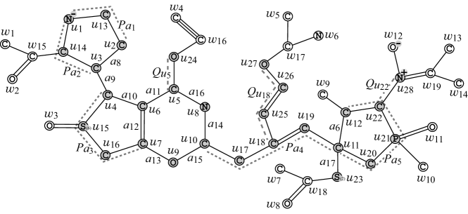
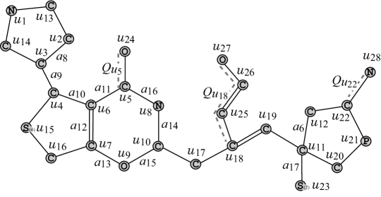
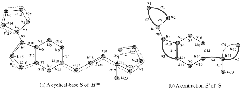
Figure 2 illustrates an example of a hydrogen-suppressed chemical graph $\langle\mathbb{C}\rangle$. For a branch-parameter ${\rho}=2$, the interior of the chemical graph $\langle\mathbb{C}\rangle$ in Figure 2 is obtained by removing the set of vertices with degree 1 ${\rho}=2$ times; i.e., first remove the set $V_{1}=\{w_{1},w_{2},\ldots,w_{14}\}$ of vertices of degree 1 in $\langle\mathbb{C}\rangle$ and then remove the set $V_{2}=\{w_{15},w_{16},\ldots,w_{19}\}$ of vertices of degree 1 in $\langle\mathbb{C}\rangle-V_{1}$, where the removed vertices become the exterior-vertices of $\langle\mathbb{C}\rangle$.

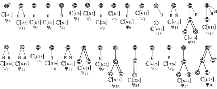
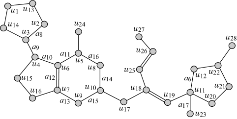
For each interior-vertex $u\in V^{\mathrm{int}}(\mathbb{C})$, let $T_{u}\in\mathcal{T}^{\mathrm{ex}}(\langle\mathbb{C}\rangle)$ denote the chemical tree rooted at $u$ (where possibly $T_{u}$ consists of vertex $u$) and define the $\rho$-fringe-tree $\mathbb{C}[u]$ to be the chemical rooted tree obtained from $T_{u}$ by putting back the hydrogens originally attached with $T_{u}$ in $\mathbb{C}$. Let $\mathcal{T}(\mathbb{C})$ denote the set of $\rho$-fringe-trees $\mathbb{C}[u],u\in V^{\mathrm{int}}(\mathbb{C})$. Figure 3 illustrates the set $\mathcal{T}(\mathbb{C})=\{\mathbb{C}[u_{i}]\mid i\in[1,28]\}$ of the 2-fringe-trees of the example $\mathbb{C}$ in Figure 2.

Figure 3: The set $\mathcal{T}(\mathbb{C})$ of 2-fringe-trees $\mathbb{C}[u_{i}],i\in[1,28]$ of the example $\mathbb{C}$ in Figure 2, where the root of each tree is depicted with a gray circle and the hydrogens attached to non-root vertices are omitted in the figure.

Feature Function  The feature of an interior-edge $e=uv\in E^{\mathrm{int}}(\mathbb{C})$ such that $\alpha(u)={\tt a}$, $\deg_{\langle\mathbb{C}\rangle}(u)=d$, $\alpha(v)={\tt b}$, $\deg_{\langle\mathbb{C}\rangle}(v)=d^{\prime}$ and $\beta(e)=m$ is represented by a tuple $({\tt a}d,{\tt b}d^{\prime},m)$, which is called the edge-configuration of the edge $e$, where we call the tuple $({\tt a},{\tt b},m)$ the adjacency-configuration of the edge $e$.

In the framework with the two-layered model, the feature vector $f$ mainly consists of the frequency of edge-configurations of the interior-edges and the frequency of chemical rooted trees among the set of chemical rooted trees $\mathbb{C}[u]$ over all interior-vertices $u$. See Appendix A for all these descriptors $x(1),x(2),\ldots,x(K_{1})$, which are called linear descriptors. We denote by $D_{\pi}^{(1)}:=\{x(k)\mid k\in[1,K_{1}]\}$ the set of descriptors constructed over a data set for a property $\pi$. Zhu et al. [28] introduced a quadratic term $x(i)x(j)$ (or $x(i)(1-x(j))$), $1\leq i\leq j\leq K_{1}$ as a new descriptor, where it is assumed that each $x(i)$ is normalized between 0 and 1. This term $x(i)x(j)$, $1\leq i\leq j\leq K_{1}$ (or $x(i)(1-x(j)),i,j\in[1,K_{1}]$) is called a quadratic descriptor and is denoted by $D_{\pi}^{(2)}:=\{x(i)x(j)\mid 1\leq i\leq j\leq K_{1}\}\cup\{x(i)(1-x(j))\mid i,j\in[1,K_{1}]\}$ the set of quadratic descriptors.

To construct a prediction function, we use the union $D_{\pi}^{(1)}\cup D_{\pi}^{(2)}$. This set of descriptors is usually excessive in constructing a prediction function, and we reduce it to a smaller set of descriptors to construct a feature function $f:\mathbb{R}^{K}\to\mathbb{R}$, where $K$ is the number of resulting descriptors. We call $\mathbb{R}^{K}$ the feature space. To reduce descriptors, we use the methods proposed by Zhu et al. [28].

Topological Specification  A topological specification $\sigma$ is described as a set of the following rules:

1. a seed graph $G_{\mathrm{C}}$ as an abstract form of a target chemical graph $\mathbb{C}$;

2. a set $\mathcal{F}$ of chemical rooted trees as candidates for a tree $\mathbb{C}[u]$ rooted at each exterior-vertex $u$ in $\mathbb{C}$; and

3. lower and upper bounds on the number of components in a target chemical graph such as chemical elements, double/triple bonds and the interior-vertices in $\mathbb{C}$.

Figure 4: (a) An illustration of a seed graph $G_{\mathrm{C}}$, where the vertices in $V_{\mathrm{C}}$ are depicted with gray circles, the edges in $E_{(\geq 2)}$ are depicted with dotted lines, the edges in $E_{(\geq 1)}$ are depicted with dashed lines, the edges in $E_{(0/1)}$ are depicted with gray bold lines and the edges in $E_{(=1)}$ are depicted with black solid lines; (b) A set $\mathcal{F}=\{\psi_{1},\psi_{2},\ldots,\psi_{30}\}\subseteq\mathcal{F}(\mathcal{C}_{\pi})$ of 30 chemical rooted trees $\psi_{i},i\in[1,30]$, where the root of each tree is depicted with a gray circle. The hydrogens attached to non-root vertices are omitted in the figure.

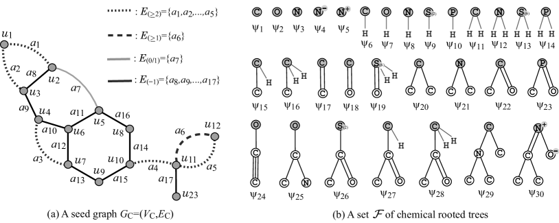
Figures 4(a) and (b) illustrate examples of a seed graph $G_{\mathrm{C}}$ and a set $\mathcal{F}$ of chemical rooted trees, respectively. Given a seed graph $G_{\mathrm{C}}$, the interior of a target chemical graph $\mathbb{C}$ is constructed from $G_{\mathrm{C}}$ by replacing some edges $a=uv$ with paths $P_{a}$ between the end-vertices $u$ and $v$ and by attaching new paths $Q_{v}$ to some vertices $v$. For example, a chemical graph $\mathbb{C}$ in Figure 2 is constructed from the seed graph $G_{\mathrm{C}}$ in Figure 4(a) as follows.

1. First replace five edges $a_{1}=u_{1}u_{2},a_{2}=u_{1}u_{3},a_{3}=u_{4}u_{7},a_{4}=u_{10}u_{11}$ and $a_{5}=u_{11}u_{12}$ in $G_{\mathrm{C}}$ with new paths $P_{a_{1}}=(u_{1},u_{13},u_{2})$, $P_{a_{2}}=(u_{1},u_{14},u_{3})$, $P_{a_{3}}=(u_{4},u_{15},u_{16},u_{7})$, $P_{a_{4}}=(u_{10},u_{17},u_{18},u_{19},u_{11})$ and $P_{a_{5}}=(u_{11},u_{20},u_{21},u_{22},u_{12})$, respectively to obtain a subgraph $G_{1}$ of $\langle\mathbb{C}\rangle$.

2. Next attach to this graph $G_{1}$ three new paths $Q_{u_{5}}=(u_{5},u_{24})$, $Q_{u_{18}}=(u_{18},u_{25},u_{26},u_{27})$ and $Q_{u_{22}}=(u_{22},u_{28})$ to obtain the interior of $\langle\mathbb{C}\rangle$ in Figure 2.

3. Finally attach to the interior 28 trees selected from the set $\mathcal{F}$ and assign chemical elements and bond-multiplicities in the interior to obtain a chemical graph $\mathbb{C}$ in Figure 2. In Figure 3, $\psi_{1}\in\mathcal{F}$ is selected for $\mathbb{C}[u_{i}]$, $i\in\{6,7,11\}$. Similarly $\psi_{2}$ for $\mathbb{C}[u_{9}]$, $\psi_{4}$ for $\mathbb{C}[u_{1}]$, $\psi_{6}$ for $\mathbb{C}[u_{i}]$, $i\in\{3,4,5,10,19,22,25,26\}$, $\psi_{8}$ for $\mathbb{C}[u_{8}]$, $\psi_{11}$ for $\mathbb{C}[u_{i}]$, $i\in\{2,13,16,17,20\}$, $\psi_{15}$ for $\mathbb{C}[u_{12}]$, $\psi_{19}$ for $\mathbb{C}[u_{15}]$, $\psi_{23}$ for $\mathbb{C}[u_{21}]$, $\psi_{24}$ for $\mathbb{C}[u_{24}]$, $\psi_{25}$ for $\mathbb{C}[u_{27}]$, $\psi_{26}$ for $\mathbb{C}[u_{23}]$, $\psi_{27}$ for $\mathbb{C}[u_{14}]$ and $\psi_{30}$ for $\mathbb{C}[u_{28}]$.

See Appendix B for a full description of topological specification.

4 Prediction Functions

Let $\mathcal{C}$ be a data set of chemical graphs $\mathbb{C}$ with an observed value $a(\mathbb{C})\in\mathbb{R}$. Let $D$ be a set of descriptors with $K=|D|$ and $f$ be a feature function that maps a chemical graph $\mathbb{C}$ to a vector $f(\mathbb{C})\in\mathbb{R}^{K}$, where $x(d)$ denotes the value of descriptor $d\in D$. For a notational simplicity, we denote $a_{i}=a(\mathbb{C}_{i})$ and $x_{i}=f(\mathbb{C}_{i})$ for an indexed graph $\mathbb{C}_{i}\in\mathcal{C}$.

4.1 Evaluation

For a prediction function $\eta:\mathbb{R}^{K}\to\mathbb{R}$, define an error function

$$\mathrm{Err}(\eta;\mathcal{C})\triangleq\sum_{\mathbb{C}_{i}\in\mathcal{C}}(a_{i}-\eta(f(\mathbb{C}_{i})))^{2}=\sum_{\mathbb{C}_{i}\in\mathcal{C}}(a_{i}-\eta(x_{i}))^{2},$$

and define the coefficient of determination $\mathrm{R}^{2}(\eta,\mathcal{C})$ to be

$${\mathrm{R}^{2}(\eta,\mathcal{C})\triangleq 1-\frac{\mathrm{Err}(\eta;\mathcal{C})}{\sum_{\mathbb{C}_{i}\in\mathcal{C}}(a_{i}-\widetilde{a})^{2}}\mbox{ for }\widetilde{a}=\frac{1}{|\mathcal{C}|}\sum_{\mathbb{C}\in\mathcal{C}}a(\mathbb{C}).}$$

We evaluate a method of constructing a prediction function over a set $D$ of descriptors by 5-fold cross-validation as follows. A single run $r$ of 5-fold cross-validation executes the following: Partition a data set $\mathcal{C}$ randomly into five subsets $\mathcal{C}^{(k)}$, $k\in[1,5]$ so that the difference between $|\mathcal{C}^{(i)}|$ and $|\mathcal{C}^{(j)}|$ is at most 1. For each $k\in[1,5]$, let $\mathcal{C}_{\mathrm{train}}:=\mathcal{C}\setminus\mathcal{C}^{(k)}$, $\mathcal{C}_{\mathrm{test}}:=\mathcal{C}^{(k)}$ and execute the method to construct a prediction function $\eta^{(k)}:\mathrm{R}^{|D|}\to\mathbb{R}$ over a training set $\mathcal{C}_{\mathrm{train}}$ and compute $g_{r}^{(k)}:=\mathrm{R}^{2}(\eta^{(k)},\mathcal{C}_{\mathrm{test}})$. Let $\mathrm{R}^{2}_{\mathrm{CV}}(\mathcal{C},D,p)$ denote the median of $\{g_{r_{i}}^{(k)}\mid k\in[1,5],i\in[1,p]\}$ of $p$ runs $r_{1},r_{2},\ldots,r_{p}$ of 5-fold cross-validation.

4.2 Linear Regressions

For a set $D$ of descriptors, a hyperplane is defined to be a pair $(w,b)$ of a vector $w\in\mathbb{R}^{K}$ and a real $b\in\mathbb{R}$. Given a hyperplane $(w,b)$, a prediction function $\eta_{w,b}:\mathbb{R}^{K}\to\mathbb{R}$ is defined by setting

$$\eta_{w,b}(x)\triangleq w\cdot x+b=\sum_{d\in D}w(d)x(d)+b.$$

Multidimensional Linear Regression (MLR)

Given a data set $\mathcal{C}$ and a set $D$ of descriptors, multidimensional linear regression MLR$(\mathcal{C},D)$ returns a hyperplane $(w,b)$ with $w\in\mathbb{R}^{K}$ that minimizes $\mathrm{Err}(\eta_{w,b};\mathcal{C})$. However, such a hyperplane $(w,b)$ may contain unnecessarily many non-zero reals $w(d)$. To avoid this, a minimization with an additional penalty term $\tau$ to the error function has been proposed. Among them, a Lasso function [26] is defined to be

$$\frac{1}{2|\mathcal{C}|}\mathrm{Err}(\eta_{w,b};\mathcal{C})+\lambda\tau,~{}~{}~{}\tau=\sum_{d\in D}|w(d)|+|b|,$$

where $\lambda\in\mathbb{R}_{+}$ is a given nonnegative number.

Adjustive Linear Regression (ALR)

We review a recent learning method, called adjustive linear regression, that is effectively equivalent to an ANN with no hidden layers by a linear regression such that each input node may have a non-linear activation function (see [27] for the details of the idea). Let $\mathcal{C}=\{\mathbb{C}_{1},\mathbb{C}_{2},\ldots,\mathbb{C}_{m}\}$, $A=\{a_{i}=f(\mathbb{C}_{i})\mid i\in[1,m]\}$ and $X=\{x_{i}=f(\mathbb{C}_{i})\in\mathbb{R}^{K}\mid i\in[1,m]\}$. Let $D^{+}$ (resp., $D^{-}$) denote the set of descriptor $d\in D$ such that the correlation coefficient $\sigma(X[d],A)$ between $X[d]=\{x_{i}(d)\mid i\in[1,m]\}$ and $A$ is nonnegative (resp., negative). We first solve the following linear program with a constant $\lambda\geq 0$, a real variable $b$ and nonnegative real variables $c_{q}(0),q\in[0,2]$, $w_{q}(d),q\in[0,2],d\in D$.

Linear Program

$$\begin{array}[]{l }\mbox{Minimize: ~{}}\displaystyle{\frac{1}{2m}\sum_{i\in[1,m]}\Bigl{|}c_{0}(0)a_{i}+c_{1}(0)a_{i}^{2}+c_{2}(0)(1-(a_{i}\!-\!1)^{2})}\\ \displaystyle{~{}~{}~{}~{}~{}~{}~{}~{}~{}~{}~{}~{}~{}~{}~{}~{}~{}~{}~{}~{}~{}~{}~{}~{}~{}~{}~{}~{}~{}-\sum_{d\in D^{+}}[w_{0}(d)x_{i}(d)+w_{1}(d)x_{i}(d)^{2}+w_{2}(d)(1-(x_{i}(d)\!-\!1)^{2})]}\\ \displaystyle{~{}~{}~{}~{}~{}~{}~{}~{}~{}~{}~{}~{}~{}~{}~{}~{}~{}~{}~{}~{}~{}~{}~{}~{}~{}~{}~{}~{}~{}+\sum_{d\in D^{-}}[w_{0}(d)x_{i}(d)+w_{1}(d)x_{i}(d)^{2}+w_{2}(d)(1-(x_{i}(d)\!-\!1)^{2})]-b\Bigr{|}+\lambda\tau}\\ \mbox{subject to}\\ ~{}~{}~{}~{}~{}~{}~{}~{}~{}~{}~{}~{}~{}~{}~{}~{}~{}~{}~{}~{}~{}\displaystyle{\tau=\sum_{d\in D}w_{0}(d)+|b|,~{}~{}~{}c_{0}(0)+c_{1}(0)+c_{2}(0)=1.}\end{array}$$ (1)

An optimal solution to this minimization can be found by solving a linear program with $O(m+|D|)$ variables and constraints. From an optimal solution, we next compute the following hyperplane $(w^{*},b^{*})$ to obtain a linear prediction function $\eta_{w^{*},b^{*}}$. Let $c^{*}_{q}(0),q\in[0,2]$, $w^{*}_{q}(d),q\in[0,2],d\in D$ and $b^{*}$ denote the values of variables $c_{q}(0),q\in[0,2]$, $w_{q}(d),q\in[0,2],d\in D$ and $b$ in an optimal solution, respectively. Let $D^{\dagger}$ denote the set of descriptors $d\in D$ with $w^{*}_{0}(d)>0$. Then we set
    $w^{*}(d):=0$ for $d\in D$ with $w^{*}_{0}(d)=0$,
    $w^{*}(d):=w^{*}_{0}(d)/(w^{*}_{0}(d)+w^{*}_{1}(d)+w^{*}_{2}(d))$ for $d\in D^{+}\cap D^{\dagger}$,
    $w^{*}(d):=-w^{*}_{0}(d)/(w^{*}_{0}(d)+w^{*}_{1}(d)+w^{*}_{2}(d))$ for $d\in D^{-}\cap D^{\dagger}$ and
    $w^{*}:=(w^{*}_{0}(1),w^{*}_{0}(2),\ldots,w^{*}_{0}(|D|))\in\mathbb{R}^{K}$.

Reduction of Descriptors and Linear Regression (RLR)

We finally review a learning method recently proposed by Zhu et al. [28] to improve the learning performance with the two-layered model. Given a set of descriptors $x(1),x(2),\ldots,x(K)$, the method first adds to the original set of linear descriptors a quadratic descriptor $x(i)x(j)$ (or $x(i)(1-x(j))$ of each two descriptors. This drastically increases the number of descriptors, which would take extra running time in learning or cause over-fitting to the data set. Next the method reduces the set of linear and quadratic descriptors into a smaller set that delivers a prediction function with a higher performance (see [28] for the details on the reduction procedure). Finally the method constructs a prediction function by using MLR on the set of selected descriptors. We call this method based on reduction and linear regression RLR in this paper.

5 Splitting Data Sets via Hyperplanes

This section proposes a method of splitting a given data set into two subsets with a hyperplane in the feature space so that most of the compounds $\mathbb{C}$ in the first (resp., second) subsets have observed values $a(\mathbb{C})$ smaller (resp., larger) than a threshold $\theta$.

For a property $\pi$, let $\mathcal{C}=\{\mathbb{C}_{1},\mathbb{C}_{2},\ldots,\mathbb{C}_{n}\}$ be a set of chemical graphs. Assume that all entries and observed values are normalized, where $\min\{a_{i}\mid\mathbb{C}_{i}\in\mathcal{C}\}=0$ and $\max\{a_{i}\mid\mathbb{C}_{i}\in\mathcal{C}\}=1$ and $\min\{x_{i}(d)\mid\mathbb{C}_{i}\in\mathcal{C}\}=0$ and $\max\{x_{i}(d)\mid\mathbb{C}_{i}\in\mathcal{C}\}=1$ for each $d\in D$.

For a threshold $\theta$ with $0<\theta<1$, we find a hyperplane $(w,b)$ with $w\in\mathbb{R}^{K}$ and $b\in\mathbb{R}$ that splits the set $\mathcal{C}$ into subsets

$$\mathcal{C}^{(1)}:=\{\mathbb{C}_{i}\in\mathcal{C}\mid wx_{i}-b\leq 0\} \mathcal{C}^{(2)}:=\{\mathbb{C}_{i}\in\mathcal{C}\mid wx_{i}-b>0\}$$ and

so that $\mathcal{C}^{(1)}$ (resp., $\mathcal{C}^{(2)}$) contains compounds $\mathbb{C}_{i}\in\mathcal{C}$ with $a_{i}\leq\theta$ (resp., $a_{i}>\theta$) as many as possible. Then we treat each of the subsets $\mathcal{C}^{(j)},j=1,2$ as a new data set and construct a prediction function $\psi_{j}$ before we obtain a prediction function to the original set $\mathcal{C}$ by combining functions $\psi_{1}$ and $\psi_{2}$.

A Linear Program Formulation to Find a Hyperplane

To find a hyperplane to split a given data set, we formulate a linear program in a similar manner of the idea by Freed and Glover [29] for separating a classification data. Define sets $\mathcal{C}_{\leq\theta}:=\{\mathbb{C}_{i}\in\mathcal{C}\mid a_{i}\leq\theta\}$ and $\mathcal{C}_{>\theta}:=\{\mathbb{C}_{i}\in\mathcal{C}\mid a_{i}>\theta\}$, and choose compounds $\mathbb{C}_{s}\in\mathcal{C}_{\leq\theta}$ with $a_{s}=0$ and $\mathbb{C}_{t}\in\mathcal{C}_{>\theta}$ with $a_{t}=1$, so that $\mathbb{C}_{s}\in\mathcal{C}^{(1)}$, $\mathbb{C}_{t}\in\mathcal{C}^{(2)}$.

A linear program is formulated as follows, where a hyperplane $(w,b)$ with $w\in\mathbb{R}^{K}$ and $b\in\mathbb{R}$ is obtained as an optimal solution to this linear program:

LP$(\theta)$
constants: $a_{i}\in\mathbb{R}$, $x_{i}\in\mathbb{R}^{K},~{}\forall\mathbb{C}_{i}\in\mathcal{C}$; indices $s$ and $t$ such that $a_{s}=0$ and $a_{t}=1$; $\theta\in\mathbb{R}$;
variables: $w\in\mathbb{R}^{K}$, $b\in\mathbb{R}$, nonnegative variables $\delta_{i}\geq 0,\forall\mathbb{C}_{i}\in\mathcal{C}$;
constraints:

$$wx_{s}-b\leq 0,$$

$$wx_{t}-b\geq 0,$$

$$\delta_{i}\geq wx_{i}-b+(a_{i}-\theta)^{2},~{}~{}~{}\forall\mathbb{C}_{i}\in\mathcal{C}_{\leq\theta},$$

$$\delta_{i}\geq-(wx_{i}-b)+(a_{i}-\theta)^{2},~{}~{}~{}\forall\mathbb{C}_{i}\in\mathcal{C}_{>\theta},$$

objective function:

$$\mbox{minimize~{}~{}}\sum_{\mathbb{C}_{i}\in\mathcal{C}}\delta_{i}.$$

The above linear program consists of $O(|D|+|\mathcal{C}|)$ variables and $O(|\mathcal{C}|)$ constraints. We solve the linear program to obtain an optimal solution $(w,b)$ and compute $\mathcal{C}^{(1)}=\{\mathbb{C}_{i}\in\mathcal{C}\mid wx_{i}-b\leq 0\}$ and $\mathcal{C}^{(2)}=\{\mathbb{C}_{i}\in\mathcal{C}\mid wx_{i}-b>0\}$. Denote

$$a_{\min}^{(j)}:=\min\{a_{i}\mid\mathbb{C}_{i}\in\mathcal{C}^{(j)}\}\mbox{ and }a_{\max}^{(j)}:=\max\{a_{i}\mid\mathbb{C}_{i}\in\mathcal{C}^{(j)}\},j=1,2,$$

where $a_{\min}^{(1)}=0$ and $a_{\max}^{(2)}=1$. When $\mathcal{C}^{(1)}=\mathcal{C}_{\leq\theta}$ and $\mathcal{C}^{(2)}=\mathcal{C}_{>\theta}$ hold, the ranges $[a_{\min}^{(1)}=0,a_{\max}^{(1)}]$ and $[a_{\min}^{(2)},a_{\max}^{(2)}=1]$ have no overlap (i.e., $a_{\max}^{(1)}\leq\theta<a_{\min}^{(2)}$). Otherwise $a_{\min}^{(2)}\leq a_{\max}^{(1)}$ holds, where even for this case, the two subsets $\mathcal{C}^{(1)}$ and $\mathcal{C}^{(2)}$ are well-separated if $a_{\min}^{(2)}$ and $a_{\max}^{(1)}$ are very close. We select a threshold $\theta$ from a set of candidates so that $a_{\max}^{(1)}-a_{\min}^{(2)}$ is minimized subject to the condition that each of $|\mathcal{C}^{(1)}|$ and $|\mathcal{C}^{(2)}|$ becomes nearly half of the original size $|\mathcal{C}|$.

Implementation in the First Phase of the Framework

In the first phase of the framework, we construct a prediction function $\psi$ to a data set $\mathcal{C}$ for a property $\pi$ and a descriptor set $D$ of a feature function $f:\mathcal{C}\to\mathbb{R}^{K}$ as follows. For a selected threshold $\theta$, we find a hyperplane $(w,b)$, $w\in\mathbb{R}^{K}$, $b\in\mathbb{R}$ as an optimal solution to the above linear program LP$(\theta)$ based on which we split $\mathcal{C}$ into subsets $\mathcal{C}^{(j)},j=1,2$. For each $j=1,2$, choose a set $\widetilde{D}_{j}$ of descriptors and construct a prediction function $\psi_{j}:\mathbb{R}^{|\widetilde{D}_{j}|}\to\mathbb{R}$ for the data set $\mathcal{C}^{(j)}$ with the descriptor set $\widetilde{D}_{j}$. In our computational experiments, we use LLR, ANN, ALR and RLR to construct prediction functions to $\mathcal{C}^{(j)},j=1,2$ and choose as $\psi_{j}$ one of them with the best learning performance (where $\widetilde{D}_{j}$ is a subset of the linear descriptor set $D$ when we use LLR, ANN or ALR; and $\widetilde{D}_{j}$ consists of some linear and quadratic descriptors of $D$ when RLR is used to construct $\psi_{j}$). Given a feature vector $x\in\mathbb{R}^{K}$, use the prediction function $\psi_{1}$ if $wx-b\leq 0$; and use the prediction function $\psi_{2}$ otherwise. Thus the prediction function $\psi$ is given by

$$\psi(x):=\left\{\begin{array}[]{ll}\psi_{1}(x)&\mbox{if $wx-b\leq 0$,}\\ \psi_{2}(x)&\mbox{otherwise,}\end{array}\right.$$

where the hyperplane $(w,b)$ is a part of the prediction function $\psi$.

Implementation in the Second Phase of the Framework

In the second phase of the framework, we need an MILP formulation that simulates the computing process of a prediction function $\psi$. Such a formulation for a prediction function constructed with LLR, ANN, ALR or RLR has been known [21, 27, 28]. For the data set $\mathcal{C}$ for property $\pi$ in the first phase, let $(w,b)$ denote the hyperplane that splits $\mathcal{C}$ into subsets $\mathcal{C}^{(j)},j=1,2$ and $\psi_{j}$ be a prediction function constructed for $\mathcal{C}^{(j)}$. Assume that, for the feature function $f$, a topological specification $\sigma$ and each prediction function $\psi_{j},j=1,2$, we have an MILP formulation $\mathcal{M}_{f,\eta_{j},\sigma}$ for inferring a chemical graph that satisfies $\sigma$ in the second phase.

Let $\underline{y}^{*}$ and $\overline{y}^{*}$ be lower and upper limits for a target value to property $\pi$. Recall that the observed value $a(\mathbb{C})$ of a chemical compound $\mathbb{C}\in\mathcal{C}$ is normalized to a value $\nu(a(\mathbb{C}))$ between 0 and 1. Let $\nu(\underline{y}^{*})$ and $\nu(\overline{y}^{*})$ denote the normalized values of $\underline{y}^{*}$ and $\overline{y}^{*}$, respectively, where we assume that either $\nu(\overline{y}^{*})\leq\max\{a_{\max}^{(1)},\theta\}$ or $\min\{a_{\min}^{(2)},\theta\}\leq\nu(\underline{y}^{*})$ (otherwise we consider two target instances $[\nu(\underline{y}^{*}),\max\{a_{\max}^{(1)},\theta\}]$ and $[\min\{a_{\min}^{(2)},\theta\},\nu(\overline{y}^{*})]$). In the former (resp., the latter), we solve the MILP $\mathcal{M}_{f,\eta_{1},\sigma}$ plus an additional constraint of $wx_{i}-b\leq 0$ (resp., MILP $\mathcal{M}_{f,\eta_{2},\sigma}$ plus an additional constraint of $wx_{i}-b\geq 0$) to infer a desired chemical graph $\mathbb{C}^{\dagger}$.

6 Results

With our new method of splitting a data set and formulating an MILP to treat quadratic descriptors in the two-layered model, we implemented the framework for inferring chemical graphs and conducted experiments to evaluate the computational efficiency. We executed the experiments on a PC with Processor: Core i7-9700 (3.0GHz; 4.7 GHz at the maximum) and Memory: 16 GB RAM DDR4. To construct a prediction function by MLR (multidimensional linear regression), or ANN (artificial neural network), we used scikit-learn version 1.0.2 with Python 3.8.12, MLPRegressor for MLR, and ReLU activation function for ANN.

6.1 Results on the First Phase of the Framework

Chemical Properties We implemented the first phase for the following 22 chemical properties of monomers:
  autoignition temperature (At), biological half life (BHL), critical pressure (Cp),
  critical temperature (Ct), dissociation constants (Dc), flammable limits lower (FlmL),
  flammable limits upper (FlmU), flash point in closed cup (Fp), melting point (Mp),
  refractive index of trees (RfIdT), odor threshold lower (OdrL), odor threshold upper (OdrU)
  and vapor pressure (Vp)
  provided by HSDB from PubChem [30];
  solubility (Sl) by ESOL [31];
  autoignition temperature for organic compounds (AtO) by A. Dashti et al. [32];
  flammable limits upper for organic compounds (FlmUO) by S. Yuan et al. [33];
  flammable limits lower for gas (FlmLG) and
  flammable limits upper for gas (FlmUG) by S. Kondo et al. [34]; and
  energy of highest occupied molecular orbital (Homo),
  energy of lowest unoccupied molecular orbital (Lumo),
  the energy difference between Homo and Lumo (Gap) and
  electric dipole moment (mu) provided by MoleculeNet [35], where all these from Homo
  to mu are based on a common data set QM9.

The data set QM9 contains more than 130,000 compounds. In our experiment, we use a set of 1,000 compounds randomly selected from the data set. We do not exclude any polymer from the original data set as outliers for these properties.

Table 1: Results of setting data sets.

$\pi$	$\Lambda$	$|\mathcal{C}_{\pi}|$	$\underline{n},~{}\overline{n}$	$\underline{a},~{}\overline{a}$	$|\Gamma|$	$|\mathcal{F}|$	$K_{1}$
At	$\lambda_{1}$	400	4, 85	64.0, 715.0	23	160	216
At	$\lambda_{3}$	448	4, 85	64.0, 715.0	28	181	254
AtO	$\lambda_{5}$	443	2, 32	170.0, 680.0	16	205	262
BHL	$\lambda_{1}$	300	5, 36	-1.522, 2.865	20	70	117
BHL	$\lambda_{3}$	514	5, 36	-1.522, 2.865	26	101	164
Cp	$\lambda_{1}$	125	4, 63	$4.7\!\times\!10^{-6}$, 5.52	8	75	107
Cp	$\lambda_{4}$	131	4, 63	$4.7\!\times\!10^{-6}$, 5.52	8	79	115
Ct	$\lambda_{1}$	125	4, 63	56.1, 3607.5	8	76	108
Ct	$\lambda_{4}$	132	4, 63	56.1, 3607.5	8	81	117
Dc	$\lambda_{1}$	141	5, 44	0.5, 17.11	20	62	109
Dc	$\lambda_{3}$	161	5, 44	0.5, 17.11	25	69	128
FlmL	$\lambda_{6}$	254	4, 67	-0.585, 0.875	19	126	177
FlmLG	$\lambda_{8}$	233	1, 13	-0.221, 1.158	10	152	199
FlmU	$\lambda_{6}$	219	4, 67	0.107, 1.681	19	119	170
FlmUO	$\lambda_{7}$	78	2, 10	0.732, 1.903	7	61	99
FlmUG	$\lambda_{7}$	233	1, 13	0.462, 2.0	10	152	199
Fp	$\lambda_{1}$	368	4, 67	-82.99, 300.0	20	131	181
Fp	$\lambda_{3}$	424	4, 67	-82.99, 300.0	25	161	228
Mp	$\lambda_{1}$	467	4, 122	-185.33, 300.0	23	142	195
Mp	$\lambda_{3}$	577	4, 122	-185.33, 300.0	32	176	253
OdrL	$\lambda_{1}$	64	4, 13	0.0002, 725.0	13	49	88
OdrL	$\lambda_{3}$	83	4, 22	0.0002, 725.0	16	60	107
OdrU	$\lambda_{1}$	64	4, 13	0.024, 6000.0	13	49	88
OdrU	$\lambda_{3}$	83	4, 22	0.015, 6000.0	16	60	107
RfIdT	$\lambda_{1}$	166	4, 26	1.3326, 1.613	14	98	139
Sl	$\lambda_{1}$	673	4, 55	-9.332, 1.11	27	154	216
Sl	$\lambda_{3}$	915	4, 55	-11.6, 1.11	42	207	299
Vp	$\lambda_{1}$	392	4, 55	-8.0, 3.416	22	133	185
Vp	$\lambda_{3}$	482	4, 55	-8.0, 3.416	30	165	236
Homo	$\lambda_{2}$	977	6, 9	-0.3335,  -0.1583	59	190	296
Lumo	$\lambda_{2}$	977	6, 9	-0.1144, 0.1026	59	190	296
Gap	$\lambda_{2}$	977	6, 9	0.1324, 0.4117	59	190	296
mu	$\lambda_{2}$	977	6, 9	0.04, 6.8966	59	190	296

Setting Data Sets For each property $\pi$, we first select a set $\Lambda$ of chemical elements and then collect a data set $\mathcal{C}_{\pi}$ on chemical graphs over the set $\Lambda$ of chemical elements. To construct the data set $\mathcal{C}_{\pi}$, we eliminated chemical compounds that do not satisfy one of the following: the graph is connected, the number of carbon atoms is at least four, and the number of non-hydrogen neighbors of each atom is at most 4.

We set a branch-parameter ${\rho}$ to be 2, introduce linear descriptors defined by the two-layered graph in the chemical model without suppressing hydrogen and use the sets $D_{\pi}^{(1)}$ and $D_{\pi}^{(2)}$ of linear and quadratic descriptors (see Appendix A for the details).

For properties $\pi\in\{$BHL, FlmL, FlmLG, FlmU, FlmUO, FlmUG, OdrL, OdrU, Vp$\}$, we take the logarithmic measurement of observed values $a(\mathbb{C}),\mathbb{C}\in\mathcal{D}_{\pi}$, where $\log(a(\mathbb{C})+c)$ ($c=10^{-8}$ if $\pi=$Vp and $c=0$ otherwise) is used as the observed value in our experiments.

We normalize the range of each linear descriptor and the range of observed values $a(\mathbb{C}),\mathbb{C}\in\mathcal{C}_{\pi}$.

We conducted an experiment of comparing the following five methods of constructing a prediction function.

1. LLR: use Lasso linear regression on the set $D_{\pi}^{(1)}$ of linear descriptors (see [21] for the detail of the implementation);

2. ANN: use ANN on the set $D_{\pi}^{(1)}$ of linear descriptors (see [21] for the detail of the implementation);

3. ALR: use adjustive linear regression on the set $D_{\pi}^{(1)}$ of linear descriptors (see [27] for the detail of the implementation);

4. RLR: the learning method proposed by Zhu et al. [28] that chooses a set of descriptors from the set $D_{\pi}^{(1)}\cup D_{\pi}^{(2)}$ of linear and quadratic descriptors and then constructs a prediction function by applying MLR (multidimensional linear regression) to the resulting set of descriptors; and

5. HPS: our method of computing a hyperplane to split a given data set into two subsets and constructing a prediction function to each subset independently. By conducting a preliminary experiment, we predetermine a threshold $\theta$ and a hyperplane $(w,b),w\in\mathbb{R}^{|D_{\pi}^{(1)}|}$ and $b\in\mathbb{R}$ in the feature space of linear descriptors. In a cross-validation, we split a training data set $\widehat{\mathcal{C}}_{\pi}\subseteq\mathcal{C}_{\pi}$ into two subsets $\widehat{\mathcal{C}}_{\pi}^{(j)},j=1,2$ and construct a prediction function $\psi_{j}$ to each subset $\widehat{\mathcal{C}}_{\pi}^{(j)}$ by applying one of the above four methods (i)-(iv).

Table 1 shows the size and range of data sets that we prepared for each chemical property to construct a prediction function, where we denote the following:

1. $\pi$: the name of a chemical property used in the experiment.

2. $\Lambda$: a set of selected elements used in the data set $\mathcal{C}_{\pi}$; $\Lambda$ is one of the following eight sets:
   $\Lambda_{1}=\{{\tt H},{\tt C},{\tt O},{\tt N}\}$; $\Lambda_{2}=\{{\tt H},{\tt C},{\tt O},{\tt N},{\tt F}\}$; $\Lambda_{3}=\{{\tt H},{\tt C},{\tt O},{\tt N},{\tt Cl},{\tt S}_{(2)},{\tt S}_{(6)}\}$; $\Lambda_{4}=\{{\tt H},{\tt C},{\tt O},{\tt N},{\tt Cl},{\tt Pb}\}$; $\Lambda_{5}=\{{\tt H},{\tt C},{\tt O},{\tt N},{\tt S}_{(2)},{\tt S}_{(4)},{\tt S}_{(6)},{\tt Cl},{\tt Br},{\tt F}\}$; $\Lambda_{6}=\{{\tt H},{\tt C},{\tt O},{\tt N},{\tt Cl},{\tt P}_{(2)},{\tt P}_{(5)}\}$; $\Lambda_{7}=\{{\tt H},{\tt C},{\tt O},{\tt N},{\tt Cl},{\tt Br}\}$; $\Lambda_{8}=\{{\tt H},{\tt C},{\tt O},{\tt N},{\tt Cl},{\tt Br},{\tt F}\}$, where ${\tt a}_{(i)}$ for a chemical element ${\tt a}$ and an integer $i\geq 1$ means that a chemical element ${\tt a}$ with valence $i$.

3. $|\mathcal{C}_{\pi}|$: the size of data set $\mathcal{C}_{\pi}$ over the element set $\Lambda$ for the property $\pi$.

4. $\underline{n},~{}\overline{n}$: the minimum and maximum values of the number $n(\mathbb{C})$ of non-hydrogen atoms in the compounds $\mathbb{C}$ in $\mathcal{C}_{\pi}$.

5. $\underline{a},~{}\overline{a}$: the minimum and maximum values of $a(\mathbb{C})$ (or the logarithm of the original observed values) for $\pi$ over the compounds $\mathbb{C}$ in $\mathcal{C}_{\pi}$ before we normalize them between 0 and 1.

6. $|\Gamma|$: the number of different edge-configurations of interior-edges over the compounds in $\mathcal{C}_{\pi}$.

7. $|\mathcal{F}|$: the number of non-isomorphic chemical rooted trees in the set of all 2-fringe-trees in the compounds in $\mathcal{C}_{\pi}$.

8. $K_{1}$: the size $|D_{\pi}^{(1)}|$ of a set $D_{\pi}^{(1)}$ of linear descriptors, where $|D_{\pi}^{(2)}|=(3K_{1}^{2}+K_{1})/2$ holds.

Constructing Prediction Functions For each chemical property $\pi$, we construct a prediction function by one of the four methods (i)-(iv).

For methods (i)-(iv), we used the same implementation due to Zhu et al. [21, 27, 28] and omit the details.

Tables 2 shows the results on constructing prediction functions, where we denote the following:

1. $\pi,\Lambda$: an instance with a chemical property $\pi$ and a set $\Lambda$ of chemical elements selected from the data set $\mathcal{C}_{\pi}$.

2. LLR: the median of test $\mathrm{R}^{2}$ in ten 5-fold cross-validations for prediction functions constructed by the method (i).

3. ANN: the median of test $\mathrm{R}^{2}$ in ten 5-fold cross-validations for prediction functions constructed by the method (ii).

4. ALR: the median of test $\mathrm{R}^{2}$ in ten 5-fold cross-validations for prediction functions constructed by the method (iii).

5. RLR: the median of test $\mathrm{R}^{2}$ in ten 5-fold cross-validations for prediction functions constructed by the method (iv).

6. HPS: the median of test $\mathrm{R}^{2}$ in ten 5-fold cross-validations for the prediction function obtained by HPS, where a prediction function is obtained by combining the prediction functions constructed for the first and second subsets.

7. the score of LLR, ANN, ALR, RLR or HPS marked with “*” indicates the best performance among the five methods for the property $\pi$;

8. $\theta$: the threshold used in HPS to split the data set $\mathcal{C}_{\pi}$.

9. $a^{(1)}_{\max},a^{(2)}_{\min}$: the maximum observed value $a(\mathbb{C})$ of a compound $\mathbb{C}\in\mathcal{C}^{(1)}$ and the minimum observed value $a(\mathbb{C})$ of a compound $\mathbb{C}\in\mathcal{C}^{(2)}$ in HPS:

10. $|\mathcal{C}^{(1)}|,|\mathcal{C}^{(2)}|$: the sizes of the first subset $\mathcal{C}^{(1)}$ and the second subset $\mathcal{C}^{(2)}$ in HPS.

11. $\mathcal{C}^{(1)}$-R²: the name of the method (one of (i)-(iv)) used to construct a prediction function to the first subset in HPS and the median of test $\mathrm{R}^{2}$ in ten 5-fold cross-validations for the prediction function over the first subset.

12. $\mathcal{C}^{(2)}$-R²: the name of the method (one of (i)-(iv)) used to construct a prediction function to the second subset in HPS and the median of test $\mathrm{R}^{2}$ in ten 5-fold cross-validations for the prediction function over the second subset.

The running time of constructing two prediction functions for subsets $\mathcal{C}^{(1)}$ and $\mathcal{C}^{(2)}$ in HPS was at most around 13 seconds. To execute RLR, selecting a subset of linear and quadratic descriptors is the most time consuming part, which took from 1162 to 44356 seconds.

Table 2: Results of constructing prediction functions for monomers.

$\pi,\Lambda$	LLR	ANN	ALR	RLR	HPS	$\theta$	$a^{(1)}_{\max},a^{(2)}_{\min}$	$|\mathcal{C}^{(1)}|,|\mathcal{C}^{(2)}|$	$\mathcal{C}^{(1)}$-R2	$\mathcal{C}^{(2)}$-R2
At, $\lambda_{1}$	0.363	0.465	0.449	0.505	*0.808	0.40	0.505, 0.293	147, 253	RLR 0.220	RLR 0.521
At, $\lambda_{3}$	0.391	0.476	0.442	0.501	*0.765	0.35	0.555, 0.178	121, 327	ANN 0.126	RLR 0.532
AtO, $\lambda_{5}$	0.710	0.715	0.716	0.829	*0.894	0.45	0.447, 0.451	223, 220	ANN 0.747	RLR 0.610
BHL, $\lambda_{1}$	0.580	0.648	0.679	0.759	*0.818	0.45	0.598, 0.259	124, 176	RLR 0.650	RLR 0.560
BHL, $\lambda_{3}$	0.688	0.751	0.706	*0.834	0.831	0.50	0.753, 0.183	240, 274	RLR 0.620	RLR 0.569
Cp, $\lambda_{1}$	0.429	0.592	0.805	0.677	*0.887	0.55	0.549, 0.562	59,  66	RLR 0.759	RLR 0.632
Cp, $\lambda_{4}$	0.559	0.768	0.546	0.841	*0.850	0.60	0.598, 0.601	68,  63	RLR 0.661	RLR 0.564
Ct, $\lambda_{1}$	0.069	0.290	0.903	*0.937	0.863	0.15	0.150, 0.151	60,  65	RLR 0.713	LLR 0.740
Ct, $\lambda_{4}$	0.037	0.236	*0.941	0.860	0.920	0.15	0.150, 0.150	61,  71	RLR 0.791	RLR 0.883
Dc, $\lambda_{1}$	0.559	0.662	0.529	0.908	*0.939	0.45	0.440, 0.456	68,  73	RLR 0.787	RLR 0.810
Dc, $\lambda_{3}$	0.574	0.628	0.534	0.829	*0.919	0.40	0.386, 0.400	78,  83	RLR 0.551	RLR 0.760
FlmL, $\lambda_{6}$	0.412	0.524	0.707	0.604	*0.833	0.50	0.499, 0.502	106, 113	RLR 0.920	RLR 0.363
FlmLG, $\lambda_{8}$	0.850	0.786	0.824	0.925	*0.935	0.25	0.243, 0.254	38,  40	RLR 0.838	RLR 0.833
FlmU, $\lambda_{6}$	0.146	0.295	0.311	0.538	*0.703	0.45	0.445, 0.451	167,   66	RLR 0.477	RLR 0.344
FlmUO, $\lambda_{7}$	0.442	0.573	0.221	0.642	*0.851	0.45	0.429, 0.455	107, 147	RLR 0.945	RLR 0.559
FlmUG, $\lambda_{7}$	0.556	0.649	0.443	0.655	*0.837	0.35	0.346, 0.363	126, 107	RLR 0.679	RLR 0.292
Fp, $\lambda_{1}$	0.607	0.742	0.653	0.899	*0.920	0.40	0.399, 0.402	178, 190	RLR 0.684	RLR 0.880
Fp, $\lambda_{3}$	0.593	0.634	0.626	0.846	*0.880	0.45	0.449, 0.452	261, 163	RLR 0.697	RLR 0.645
Mp, $\lambda_{1}$	0.815	0.840	0.850	0.873	*0.923	0.50	0.493, 0.504	272, 195	RLR 0.607	RLR 0.778
Mp, $\lambda_{3}$	0.786	0.843	0.803	0.898	*0.920	0.55	0.547, 0.542	329, 248	ANN 0.659	RLR 0.747
OdrL, $\lambda_{1}$	-0.034	-0.402	-0.098	0.449	*0.901	0.50	0.498, 0.503	29,  35	RLR 0.695	RLR 0.836
OdrL, $\lambda_{3}$	-0.055	-0.172	0.041	0.532	*0.827	0.50	0.498, 0.503	38,  45	RLR 0.543	RLR 0.657
OdrU, $\lambda_{1}$	0.008	0.170	0.214	0.641	*0.931	0.55	0.541, 0.550	32,  32	RLR 0.755	RLR 0.800
OdrU, $\lambda_{3}$	0.164	0.266	0.392	0.654	*0.955	0.50	0.496, 0.500	40,  43	RLR 0.936	RLR 0.749
RfIdT, $\lambda_{1}$	0.679	0.770	0.677	*0.876	*0.876	0.30	0.294, 0.303	89,  77	RLR 0.873	RLR 0.594
Sl, $\lambda_{1}$	0.771	0.831	0.788	0.894	*0.923	0.45	0.449, 0.439	109, 564	RLR 0.781	RLR 0.847
Sl, $\lambda_{3}$	0.807	0.867	0.813	0.897	*0.916	0.50	0.548, 0.500	128, 787	RLR 0.859	RLR 0.832
Vp, $\lambda_{1}$	0.871	0.937	0.893	0.969	*0.986	0.45	0.449, 0.453	155, 237	RLR 0.930	RLR 0.949
Vp, $\lambda_{3}$	0.830	0.922	0.871	0.959	*0.977	0.45	0.449, 0.453	210, 272	RLR 0.845	RLR 0.935
Gap, $\lambda_{2}$	0.784	0.763	0.744	0.876	*0.907	0.25	0.298, 0.162	131, 846	RLR 0.524	RLR 0.863
Homo, $\lambda_{2}$	0.704	0.608	0.657	0.804	*0.847	0.65	0.792, 0.557	849, 128	RLR 0.733	RLR 0.768
Lumo, $\lambda_{2}$	0.841	0.843	0.819	0.920	*0.948	0.70	0.700, 0.701	700, 277	RLR 0.874	RLR 0.855
mu, $\lambda_{2}$	0.366	0.442	0.399	0.645	*0.708	0.20	0.506, 0.021	169, 808	RLR 0.708	RLR 0.593

In Table 2, HPS attains the best score of the median test R² among the five methods in most cases. Especially the improvement over the methods (i)-(iv) is significant for properties At, FlmL, FlmU, FlmUO, FlmUG, OdrL and OdrU.

From the values $a^{(1)}_{\max},a^{(2)}_{\min}$ in Table 2, we see how the original set $\mathcal{C}_{\pi}$ is split with a hyperplane into two subsets $\mathcal{C}^{(j)},j=1,2$ for each property $\pi$. For property At with $\lambda_{1}$, it holds that $a^{(1)}_{\max}=0.505>a^{(2)}_{\min}=0.293$, which implies that no hyperplane separates $\mathcal{C}_{\leq\theta}=\{\mathbb{C}_{i}\in\mathcal{C}_{\pi}\mid a_{i}\leq\theta\}$ and $\mathcal{C}_{>\theta}=\{\mathbb{C}_{i}\in\mathcal{C}_{\pi}\mid a_{i}>\theta\}$ for $\theta=0.40$. On the other hand, for property AtO, it holds that $a^{(1)}_{\max}=0.447<\theta=0.45<a^{(2)}_{\min}=0.451$, which implies that $\mathcal{C}_{\pi}$ is split with a hyperplane into $\mathcal{C}^{(1)}=\mathcal{C}_{\leq\theta}$ and $\mathcal{C}^{(2)}=\mathcal{C}_{>\theta}$.

For some properties such as At with $\lambda_{1}$, the median R² of HPS is considerably larger than the median R² of $\mathcal{C}^{(1)}$-R² and $\mathcal{C}^{(2)}$-R². For property $\pi=$ At with $\lambda_{1}$, the median R² of HPS is 0.808 whereas that of $\mathcal{C}^{(1)}$ (resp., $\mathcal{C}^{(2)}$) is 0.220 (resp., 0.521). This can happen because the range $[a_{\min}^{(1)}=0,a_{\max}^{(1)}=0.505]$ (resp., $[a_{\min}^{(2)}=0.293,a_{\max}^{(2)}=1]$) of observed values for $\mathcal{C}^{(1)}$ (resp., $\mathcal{C}^{(2)}$) is again normalized to $[0,1]$ on which a prediction function $\psi_{1}$ (resp., $\psi_{2}$) is constructed and its learning performance $\mathcal{C}^{(1)}$-R² (resp., $\mathcal{C}^{(2)}$-R²) is evaluated. However, in the evaluation of $\psi$ for the median R² of HPS, the error caused by each of the prediction functions $\psi_{j},j=1,2$ is measured as a relatively smaller value over the original wider range of observed values to $\mathcal{C}_{\pi}$.

6.2 Results on the Second Phase of the Framework

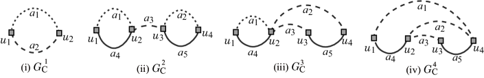
To execute the second phase, we used a set of seven instances $I_{\mathrm{a}}$, $I_{\mathrm{b}}^{i},i\in[1,4]$, $I_{\mathrm{c}}$ and $I_{\mathrm{d}}$ based on the seed graphs prepared by Zhu et al. [21]. The instances $I_{\mathrm{a}}$ and $I_{\mathrm{c}}$ have restricted seed graphs, the instances $I_{\mathrm{b}}^{i}$ have abstract seed graphs and instances $I_{\mathrm{c}}$ and $I_{\mathrm{d}}$ have restricted set of fringe-trees. We here present their seed graphs $G_{\mathrm{C}}$ (see Appendix B for the details of $I_{\mathrm{a}}$ and Appendix C for the details of $I_{\mathrm{b}}^{i},i\in[1,4]$, $I_{\mathrm{c}}$ and $I_{\mathrm{d}}$).

The seed graph $G_{\mathrm{C}}$ of $I_{\mathrm{a}}$ is given by the graph in Figure 4(a). The seed graph $G_{\mathrm{C}}^{1}$ of $I_{\mathrm{b}}^{1}$ (resp., $G_{\mathrm{C}}^{i},i=2,3,4$ of $I_{\mathrm{b}}^{i},i=2,3,4$) is illustrated in Figure 5.

Figure 5: (i) Seed graph $G_{\mathrm{C}}^{1}$ for $I_{\mathrm{b}}^{1}$ and $I_{\mathrm{d}}$; (ii) Seed graph $G_{\mathrm{C}}^{2}$ for $I_{\mathrm{b}}^{2}$; (iii) Seed graph $G_{\mathrm{C}}^{3}$ for $I_{\mathrm{b}}^{3}$; (iv) Seed graph $G_{\mathrm{C}}^{4}$ for $I_{\mathrm{b}}^{4}$.

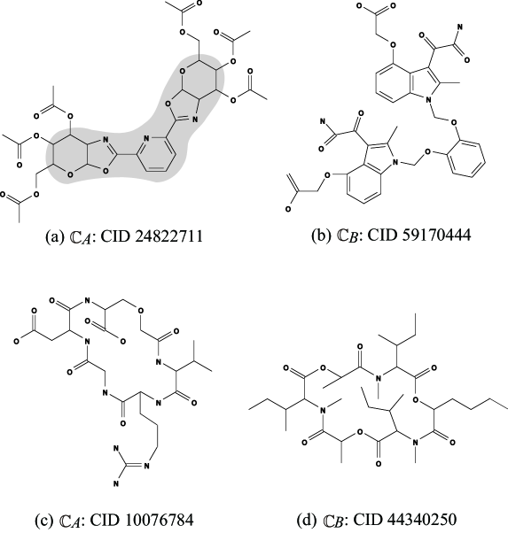
Instance $I_{\mathrm{c}}$ has been introduced in order to infer a chemical graph $\mathbb{C}^{\dagger}$ such that
- a core part of $\mathbb{C}^{\dagger}$ is equal to that of chemical graph $\mathbb{C}_{A}$: CID 24822711 in Figure 6(a)
  (where the seed graph $G_{\mathrm{C}}$ of $I_{\mathrm{c}}$ is indicated by the shaded area in Figure 6(a)).
- the frequency of each edge-configuration in the non-core of $\mathbb{C}^{\dagger}$ is equal to that of chemical graph
  $\mathbb{C}_{B}$: CID 59170444 in Figure 6(b).

Instance $I_{\mathrm{d}}$ has been introduced in order to infer a chemical graph $\mathbb{C}^{\dagger}$ such that
- $\mathbb{C}^{\dagger}$ is monocyclic (where the seed graph of $I_{\mathrm{d}}$ is given by $G_{\mathrm{C}}^{1}$ in Figure 5(i)); and
- the frequency vector of edge-configurations in $\mathbb{C}^{\dagger}$ is a vector obtained by merging those of
  chemical graphs $\mathbb{C}_{A}$: CID 10076784 and $\mathbb{C}_{B}$: CID 44340250 in Figure 6(c) and (d), respectively.

Figure 6: An illustration of chemical compounds for instances $I_{\rm c}$ and $I_{\rm d}$: (a) $\mathbb{C}_{A}$: CID 24822711; (b) $\mathbb{C}_{B}$: CID 59170444; (c) $\mathbb{C}_{A}$: CID 10076784; (d) $\mathbb{C}_{B}$: CID 44340250, where hydrogens are omitted.

Solving an MILP for the Inverse Problem We executed the stage of solving an MILP to infer a chemical graph for two properties $\pi\in\{$At, FlmL$\}$.

For the MILP formulation $\mathcal{M}_{f,\eta,\sigma}$, we use the prediction function $\eta$ for each of At with $\Lambda_{3}$ and FlmL with $\Lambda_{6}$ constructed by method (v), HPS that attained the median test $\mathrm{R}^{2}$ in Table 2. To solve an MILP with the formulation, we used CPLEX version 12.10. Tables 3 and 4 show the computational results of the experiment in this stage for the two properties, where we denote the following:

1. $n_{\mathrm{LB}}$: a lower bound on the number of non-hydrogen atoms in a chemical graph $\mathbb{C}$ to be inferred;

2. $\underline{y}^{*},~{}\overline{y}^{*}$: lower and upper bounds $\underline{y}^{*},\overline{y}^{*}\in\mathbb{R}$ on the value $a(\mathbb{C})$ of a chemical graph $\mathbb{C}$ to be inferred; For At, we use range of the original values $a(\mathbb{C})$ before normalization. For FlmL, we use the logarithmic scale $\log a(\mathbb{C})$ as the range of target values.

3. $\#$v (resp., $\#$c): the number of variables (resp., constraints) in the MILP;

4. I-time: the time (sec.) to solve the MILP;

5. $n$: the number $n(\mathbb{C}^{\dagger})$ of non-hydrogen atoms in the chemical graph $\mathbb{C}^{\dagger}$ inferred by solving the MILP;

6. $\mathrm{n}^{\mathrm{int}}$: the number $\mathrm{n}^{\mathrm{int}}(\mathbb{C}^{\dagger})$ of interior-vertices in the inferred chemical graph $\mathbb{C}^{\dagger}$; and

7. $\eta$: the predicted property value $\eta(f(\mathbb{C}^{\dagger}))$ of the inferred chemical graph $\mathbb{C}^{\dagger}$.

Table 3: Results of inferring a chemical graph $\mathbb{C}^{\dagger}$ and generating recombination solutions for At with $\Lambda_{3}$.

inst.	$n_{\mathrm{LB}}$	$\underline{y}^{*},~{}\overline{y}^{*}$	$\#$v	$\#$c	I-time	$n$	​​$\mathrm{n}^{\mathrm{int}}$	$\eta$ ​​	D-time	$\mathbb{C}$-LB	$\#\mathbb{C}$
$I_{\mathrm{a}}$	30	240, 250	9846	9250	3.61	44	25	241.98	0.111	12	12
$I_{\mathrm{b}}^{1}$	35	240, 250	10428	6904	3.07	37	15	247.71	0.0481	8	8
$I_{\mathrm{b}}^{2}$	45	240, 250	13113	10019	12.8	50	25	241.51	0.155	432	100
$I_{\mathrm{b}}^{3}$	45	190, 200	12909	10022	10.3	50	25	197.34	0.267	208	100
$I_{\mathrm{b}}^{4}$	45	300, 310	12705	10025	12.1	48	29	300.18	0.192	432	100
$I_{\mathrm{c}}$	50	360, 370	7875	8734	1.29	50	33	361.62	0.0163	1	1
$I_{\mathrm{d}}$	40	230, 240	5479	6775	2.88	43	23	237.72	0.184	10496	100

Table 4: Results of inferring a chemical graph $\mathbb{C}^{\dagger}$ and generating recombination solutions for FlmL with $\Lambda_{6}$.

inst.	$n_{\mathrm{LB}}$	$~{}\underline{y}^{*},~{}\overline{y}^{*}$	$\#$v	$\#$c	I-time	$n$	​​$\mathrm{n}^{\mathrm{int}}$	$\eta$ ​​	D-time	$\mathbb{C}$-LB	$\#\mathbb{C}$
$I_{\mathrm{a}}$	30	-0.55, -0.5	11794	12922	4.17	38	23	-0.551	0.0692	1	1
$I_{\mathrm{b}}^{1}$	35	-0.15, -0.1	11107	10423	2.82	35	9	-0.140	0.0163	2	2
$I_{\mathrm{b}}^{2}$	45	-0.5, -0.45	13426	13871	28.6	50	28	-0.494	12.8	207594	100
$I_{\mathrm{b}}^{3}$	45	-0.5, -0.45	12974	13535	20.2	45	25	-0.483	17.2	2215023	100
$I_{\mathrm{b}}^{4}$	45	-0.45, -0.4	12746	13534	12.5	46	27	-0.445	0.0889	5040	100
$I_{\mathrm{c}}$	50	-0.55, -0.5	9386	11000	0.878	50	33	-0.509	0.0162	1	1
$I_{\mathrm{d}}$	40	0.2, 0.25	6184	7821	9.18	44	23	0.204	0.16	21600	100

Figure 7(a) illustrates the chemical graph $\mathbb{C}^{\dagger}$ inferred from $I_{\mathrm{c}}$ with $(\underline{y}^{*},\overline{y}^{*})=(360,370)$ of At in Table 3.

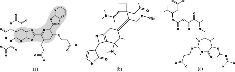
Figure 7(b) (resp., Figure 7(c)) illustrates the chemical graph $\mathbb{C}^{\dagger}$ inferred from $I_{\mathrm{a}}$ with $(\underline{y}^{*},\overline{y}^{*})=(-0.55,-0.5)$ (resp., $I_{\mathrm{d}}$ with $(\underline{y}^{*},\overline{y}^{*})=(0.2,0.25)$) of FlmL in Table 4.

Figure 7:

From Tables 3 and 4, we observe that an instance with a large number of variables and constraints takes more running time than those with a smaller size in general. All instances in this experiment are solved in a few seconds to around 30 seconds with our MILP formulation.

Generating Recombination Solutions Let $\mathbb{C}^{\dagger}$ be a chemical graph obtained by solving the MILP $\mathcal{M}_{f,\eta,\sigma}$ for the inverse problem. We here execute a stage of generating recombination solutions $\mathbb{C}^{*}\in\mathcal{G}_{\sigma}$ of $\mathbb{C}^{\dagger}$ such that $f(\mathbb{C}^{*})=x^{*}=f(\mathbb{C}^{\dagger})$.

We execute an algorithm for generating chemical isomers of $\mathbb{C}^{\dagger}$ up to 100 when the number of all chemical isomers exceeds 100. For this, we use a dynamic programming algorithm [21]. The algorithm first decomposes $\mathbb{C}^{\dagger}$ into a set of acyclic chemical graphs, next replaces each acyclic chemical graph $T$ with another acyclic chemical graph $T^{\prime}$ that admits the same feature vector as that of $T$ and finally assembles the resulting acyclic chemical graphs into a chemical isomer $\mathbb{C}^{*}$ of $\mathbb{C}^{\dagger}$. The algorithm can compute a lower bound on the total number of all chemical isomers $\mathbb{C}^{\dagger}$ without generating all of them.

Tables 3 and 4 show the computational results of the experiment in this stage for the two properties $\pi\in\{$At, FlmL$\}$, where we denote the following:

1. D-time: the running time (sec.) to execute the dynamic programming algorithm to compute a lower bound on the number of all chemical isomers $\mathbb{C}^{*}$ of $\mathbb{C}^{\dagger}$ and generate all (or up to 100) chemical isomers $\mathbb{C}^{*}$;

2. $\mathbb{C}$-LB: a lower bound on the number of all chemical isomers $\mathbb{C}^{*}$ of $\mathbb{C}^{\dagger}$; and

3. $\#\mathbb{C}$: the number of all (or up to 100) chemical isomers $\mathbb{C}^{*}$ of $\mathbb{C}^{\dagger}$ generated in this stage.

From Tables 3 and 4, we observe the running time and the number of generated recombination solutions in this stage.

For the tested properties, the chemical graph $\mathbb{C}^{\dagger}$ in $I_{\mathrm{b}}^{2}$, $I_{\mathrm{b}}^{3}$ and $I_{\mathrm{d}}$ admits a large number of chemical isomers $\mathbb{C}^{*}$, where a lower bound $\mathbb{C}$-LB on the number of chemical isomers is derived without generating all of them. The running time for computing the lower bound and generating up to 100 target chemical graphs is at most 18 second. For some chemical graphs $\mathbb{C}^{\dagger}$, the number of chemical isomers found by our algorithm was small. This is because some of acyclic chemical graphs in the decomposition of $\mathbb{C}^{\dagger}$ has no alternative acyclic chemical graph other than the original one.

Generating Neighbor Solutions Let $\mathbb{C}^{\dagger}$ be a chemical graph obtained by solving the MILP $\mathcal{M}_{f,\eta,\sigma}$ for the inverse problem. We executed a stage of generating neighbor solutions of $\mathbb{C}^{\dagger}$.

We select an MILP for the inverse problem with a prediction function $\eta$ such that a solution $\mathbb{C}^{\dagger}$ of the MILP admits only two isomers $\mathbb{C}^{*}$ in the stage of generating recombination solutions; i.e., instance $I_{\mathrm{c}}$ for property At with $\Lambda_{3}$ and instances $I_{\mathrm{a}}$, $I_{\mathrm{b}}^{4}$ and $I_{\mathrm{c}}$ for property FlmL with $\Lambda_{6}$.

In this experiment, we add to the MILP $\mathcal{M}_{f,\eta,\sigma}$ an additional set $\Theta$ of two linear constraints on linear and quadratic descriptors as follows. For the two constraints, we use the prediction functions $\eta_{\pi}$ constructed by RLR for properties $\pi\in\{$Mp, Sl$\}$ with $\Lambda_{3}$ in Table 2.

We regard each of $\eta_{\mbox{\tiny{\sc Mp}}}$ and $\eta_{\mbox{\tiny{\sc Sl}}}$ as a function from $\mathbb{R}^{|D^{\mathrm{union}}_{\pi}|}$ to $\mathbb{R}$ for $\pi\in\{$At, FlmL$\}$. We set $p_{\mathrm{dim}}:=2$ and let $\Theta$ consist of two linear constraints $\theta_{1}:=\eta_{\mbox{\tiny{\sc Mp}}}$ and $\theta_{2}:=\eta_{\mbox{\tiny{\sc Sl}}}$. We select $\delta\in\{0.01,0.05,0.1,0.15\}$ which defines a two-dimensional grid space where $\mathbb{C}^{\dagger}$ is mapped to the origin (see [23] for the detail on the neighbors). We choose a set $N_{0}$ of 48 neighbors of the origin $\mathbb{C}^{\dagger}$ in the grid search space. For each instance, we check the feasibility of neighbors in $N_{0}$ in a non-decreasing order of the distance between the neighbor and the origin. For each feasible neighbor $z\in N_{0}$, output a feasible solution $\mathbb{C}^{\dagger}_{z}$ of the augmented MILP instance. We set a time limit for checking the feasibility of a neighbor to be 300 seconds, and we skip a neighbor when the corresponding MILP is not solved within the time limit. We also ignore any neighbor $z\in N_{0}$ without testing the feasibility of $z$ if we find an infeasible neighbor $z^{\prime}\in N_{0}$ such that $z^{\prime}$ is closer to the origin than $z$ is.

Table 5 shows the computational results of the experiment for the three instances, where we denote the following:

1. (inst., $\pi$): topological specification $I$ and property $\pi$;

2. $n$: the number of non-hydrogen atoms in the tested instance;

3. $\delta$: the size of a sub-region in the grid search space;

4. #sol: the number of new chemical graphs obtained from the neighbor set $N_{0}$;

5. #infs: the number of neighbors in $N_{0}$ that are found to be infeasible during the search procedure;

6. #ign: the number of neighbors in $N_{0}$ that are ignored during the search procedure;

7. #TO: the number of neighbors in $N_{0}$ such that the time for feasibility check exceeds the time limit of 300 seconds during the search procedure.

Table 5: Results of generating neighbor solutions of $\mathbb{C}^{\dagger}$.

(inst., $\pi$)	$n$	$\delta$	#sol	#infs	#ign	#TO
($I_{\mathrm{c}}$,At)	50	0.01	9	0	0	39
($I_{\mathrm{a}}$,FlmL)	30	0.05	41	0	0	7
($I_{\mathrm{b}}^{4}$,FlmL)	45	0.15	38	0	0	10
($I_{\mathrm{c}}$,FlmL)	40	0.05	15	0	0	33

In many solvers such as CPLEX, an MILP is solved by an algorithm based on the branch-and-bound method, which sometimes takes an extremely large execution time for the same size of instances. We introduce a time limit to bound a running time of testing the feasibility of neighbors in $N_{0}$ to skip such instances. From Table 5, we observe that some number of neighbor solutions of $\mathbb{C}^{\dagger}$ could be successfully generated for each of the four instances.

7 Concluding Remarks

In the framework of inferring chemical graphs, the descriptors of a prediction function were mainly defined to be the frequencies of local graph structures in the two-layered model and defining descriptors in such a way is important to derive a compact MILP formulation in the second phase of the framework . To improve the performance of prediction functions based on the same definition of descriptors, this paper proposed a method of splitting a given data set into two subsets by a hyperplane in the feature space so that the first and second subsets mainly consist of compounds with observed values lower and higher than a threshold, respectively. A prediction function is obtained by combining prediction functions for the first and second subsets constructed independently, where the hyperplane is used to decide which of the two prediction functions is applied for a given feature vector. Our experimental results show that the proposed method improved the learning performance of chemical properties such as flammable limits and odor threshold and that the MILP in the second phase is solvable for instances of inferring a chemical graph with around 50 non-hydrogen atoms. It is left as a future work to extend our new method of splitting a data set so that a given data set is repeatedly split into smaller subsets with a narrower range of observed values when the size of the data set is large enough.

Appendix

Appendix A A Full Description of Descriptors

Associated with the two functions $\alpha$ and $\beta$ in a chemical graph $\mathbb{C}=(H,\alpha,\beta)$, we introduce functions $\mathrm{ac}:V(E)\to(\Lambda\setminus\{{\tt H}\})\times(\Lambda\setminus\{{\tt H}\})\times[1,3]$, $\mathrm{cs}:V(E)\to(\Lambda\setminus\{{\tt H}\})\times[1,6]$ and $\mathrm{ec}:V(E)\to((\Lambda\setminus\{{\tt H}\})\times[1,6])\times((\Lambda\setminus\{{\tt H}\})\times[1,6])\times[1,3]$ in the following.

To represent a feature of the exterior of $\mathbb{C}$, a chemical rooted tree in $\mathcal{T}(\mathbb{C})$ is called a fringe-configuration of $\mathbb{C}$.

We also represent leaf-edges in the exterior of $\mathbb{C}$. For a leaf-edge $uv\in E(\langle\mathbb{C}\rangle)$ with $\deg_{\langle\mathbb{C}\rangle}(u)=1$, we define the adjacency-configuration of $e$ to be an ordered tuple $(\alpha(u),\alpha(v),\beta(uv))$. Define

$$\Gamma_{\mathrm{ac}}^{\mathrm{lf}}\triangleq\{({\tt a},{\tt b},m)\mid{\tt a},{\tt b}\in\Lambda,m\in[1,\min\{\mathrm{val}({\tt a}),\mathrm{val}({\tt b})\}]\}$$

as a set of possible adjacency-configurations for leaf-edges.

To represent a feature of an interior-vertex $v\in V^{\mathrm{int}}(\mathbb{C})$ such that $\alpha(v)={\tt a}$ and $\deg_{\langle\mathbb{C}\rangle}(v)=d$ (i.e., the number of non-hydrogen atoms adjacent to $v$ is $d$) in a chemical graph $\mathbb{C}=(H,\alpha,\beta)$, we use a pair $({\tt a},d)\in(\Lambda\setminus\{{\tt H}\})\times[1,4]$, which we call the chemical symbol $\mathrm{cs}(v)$ of the vertex $v$. We treat $({\tt a},d)$ as a single symbol ${\tt a}d$, and define $\Lambda_{\mathrm{dg}}$ to be the set of all chemical symbols $\mu={\tt a}d\in(\Lambda\setminus\{{\tt H}\})\times[1,4]$.

We define a method for featuring interior-edges as follows. Let $e=uv\in E^{\mathrm{int}}(\mathbb{C})$ be an interior-edge $e=uv\in E^{\mathrm{int}}(\mathbb{C})$ such that $\alpha(u)={\tt a}$, $\alpha(v)={\tt b}$ and $\beta(e)=m$ in a chemical graph $\mathbb{C}=(H,\alpha,\beta)$. To feature this edge $e$, we use a tuple $({\tt a},{\tt b},m)\in(\Lambda\setminus\{{\tt H}\})\times(\Lambda\setminus\{{\tt H}\})\times[1,3]$, which we call the adjacency-configuration $\mathrm{ac}(e)$ of the edge $e$. We introduce a total order $<$ over the elements in $\Lambda$ to distinguish between $({\tt a},{\tt b},m)$ and $({\tt b},{\tt a},m)$ $({\tt a}\neq{\tt b})$ notationally. For a tuple $\nu=({\tt a},{\tt b},m)$, let $\overline{\nu}$ denote the tuple $({\tt b},{\tt a},m)$.

Let $e=uv\in E^{\mathrm{int}}(\mathbb{C})$ be an interior-edge $e=uv\in E^{\mathrm{int}}(\mathbb{C})$ such that $\mathrm{cs}(u)=\mu$, $\mathrm{cs}(v)=\mu^{\prime}$ and $\beta(e)=m$ in a chemical graph $\mathbb{C}=(H,\alpha,\beta)$. To feature this edge $e$, we use a tuple $(\mu,\mu^{\prime},m)\in\Lambda_{\mathrm{dg}}\times\Lambda_{\mathrm{dg}}\times[1,3]$, which we call the edge-configuration $\mathrm{ec}(e)$ of the edge $e$. We introduce a total order $<$ over the elements in $\Lambda_{\mathrm{dg}}$ to distinguish between $(\mu,\mu^{\prime},m)$ and $(\mu^{\prime},\mu,m)$ $(\mu\neq\mu^{\prime})$ notationally. For a tuple $\gamma=(\mu,\mu^{\prime},m)$, let $\overline{\gamma}$ denote the tuple $(\mu^{\prime},\mu,m)$.

Let $\pi$ be a chemical property for which we will construct a prediction function $\eta$ from a feature vector $f(\mathbb{C})$ of a chemical graph $\mathbb{C}$ to a predicted value $y\in\mathbb{R}$ for the chemical property of $\mathbb{C}$.

We first choose a set $\Lambda$ of chemical elements and then collect a data set $\mathcal{C}_{\pi}$ of chemical compounds $C$ whose chemical elements belong to $\Lambda$, where we regard $\mathcal{C}_{\pi}$ as a set of chemical graphs $\mathbb{C}$ that represent the chemical compounds $C$ in $\mathcal{C}_{\pi}$. To define the interior/exterior of chemical graphs $\mathbb{C}\in\mathcal{C}_{\pi}$, we next choose a branch-parameter ${\rho}$, where we recommend ${\rho}=2$.

Let $\Lambda^{\mathrm{int}}(\mathcal{C}_{\pi})\subseteq\Lambda$ (resp., $\Lambda^{\mathrm{ex}}(\mathcal{C}_{\pi})\subseteq\Lambda$) denote the set of chemical elements used in the set $V^{\mathrm{int}}(\mathbb{C})$ of interior-vertices (resp., the set $V^{\mathrm{ex}}(\mathbb{C})$ of exterior-vertices) of $\mathbb{C}$ over all chemical graphs $\mathbb{C}\in\mathcal{C}_{\pi}$, and $\Gamma^{\mathrm{int}}(\mathcal{C}_{\pi})$ denote the set of edge-configurations used in the set $E^{\mathrm{int}}(\mathbb{C})$ of interior-edges in $\mathbb{C}$ over all chemical graphs $\mathbb{C}\in\mathcal{C}_{\pi}$. Let $\mathcal{F}(\mathcal{C}_{\pi})$ denote the set of chemical rooted trees $\psi$ r-isomorphic to a chemical rooted tree in $\mathcal{T}(\mathbb{C})$ over all chemical graphs $\mathbb{C}\in\mathcal{C}_{\pi}$, where possibly a chemical rooted tree $\psi\in\mathcal{F}(\mathcal{C}_{\pi})$ consists of a single chemical element ${\tt a}\in\Lambda\setminus\{{\tt H}\}$.

We define an integer encoding of a finite set $A$ of elements to be a bijection $\sigma:A\to[1,|A|]$, where we denote by $[A]$ the set $[1,|A|]$ of integers. Introduce an integer coding of each of the sets $\Lambda^{\mathrm{int}}(\mathcal{C}_{\pi})$, $\Lambda^{\mathrm{ex}}(\mathcal{C}_{\pi})$, $\Gamma^{\mathrm{int}}(\mathcal{C}_{\pi})$ and $\mathcal{F}(\mathcal{C}_{\pi})$. Let $[{\tt a}]^{\mathrm{int}}$ (resp., $[{\tt a}]^{\mathrm{ex}}$) denote the coded integer of an element ${\tt a}\in\Lambda^{\mathrm{int}}(\mathcal{C}_{\pi})$ (resp., ${\tt a}\in\Lambda^{\mathrm{ex}}(\mathcal{C}_{\pi})$), $[\gamma]$ denote the coded integer of an element $\gamma$ in $\Gamma^{\mathrm{int}}(\mathcal{C}_{\pi})$ and $[\psi]$ denote an element $\psi$ in $\mathcal{F}(\mathcal{C}_{\pi})$.

Over 99% of chemical compounds $\mathbb{C}$ with up to 100 non-hydrogen atoms in PubChem have degree at most 4 in the hydrogen-suppressed graph $\langle\mathbb{C}\rangle$ [24]. We assume that a chemical graph $\mathbb{C}$ treated in this paper satisfies $\deg_{\langle\mathbb{C}\rangle}(v)\leq 4$ in the hydrogen-suppressed graph $\langle\mathbb{C}\rangle$.

In our model, we use an integer $\mathrm{mass}^{*}({\tt a})=\lfloor 10\cdot\mathrm{mass}({\tt a})\rfloor$, for each ${\tt a}\in\Lambda$.

For a chemical property $\pi$, we define a set $D_{\pi}^{(1)}$ of descriptors of a chemical graph $\mathbb{C}=(H,\alpha,\beta)\in\mathcal{C}_{\pi}$ to be the following non-negative integers $\mathrm{dcp}_{i}(\mathbb{C})$, $i\in[1,K_{1}]$, where $K_{1}=14+|\Lambda^{\mathrm{int}}(\mathcal{C}_{\pi})|+|\Lambda^{\mathrm{ex}}(\mathcal{C}_{\pi})|+|\Gamma^{\mathrm{int}}(\mathcal{C}_{\pi})|+|\mathcal{F}(\mathcal{C}_{\pi})|+|\Gamma_{\mathrm{ac}}^{\mathrm{lf}}|$.

1. $\mathrm{dcp}_{1}(\mathbb{C})$: the number $|V(H)|-|V_{\tt H}|$ of non-hydrogen atoms in $\mathbb{C}$.

2. $\mathrm{dcp}_{2}(\mathbb{C})$: the rank of $\mathbb{C}$ (i.e., the minimum number of edges to be removed to make the graph acyclic).

3. $\mathrm{dcp}_{3}(\mathbb{C})$: the number $|V^{\mathrm{int}}(\mathbb{C})|$ of interior-vertices in $\mathbb{C}$.

4. $\mathrm{dcp}_{4}(\mathbb{C})$: the average $\overline{\mathrm{ms}}(\mathbb{C})$ of mass^∗ over all atoms in $\mathbb{C}$;
   i.e., $\overline{\mathrm{ms}}(\mathbb{C})\triangleq\frac{1}{|V(H)|}\sum_{v\in V(H)}\mathrm{mass}^{*}(\alpha(v))$.

5. $\mathrm{dcp}_{i}(\mathbb{C})$, $i=4+d,d\in[1,4]$: the number $\mathrm{dg}_{d}^{\overline{{\tt H}}}(\mathbb{C})$ of non-hydrogen vertices $v\in V(H)\setminus V_{\tt H}$ of degree $\deg_{\langle\mathbb{C}\rangle}(v)=d$ in the hydrogen-suppressed chemical graph $\langle\mathbb{C}\rangle$.

6. $\mathrm{dcp}_{i}(\mathbb{C})$, $i=8+d,d\in[1,4]$: the number $\mathrm{dg}_{d}^{\mathrm{int}}(\mathbb{C})$ of interior-vertices of interior-degree $\deg_{\mathbb{C}^{\mathrm{int}}}(v)=d$ in the interior $\mathbb{C}^{\mathrm{int}}=(V^{\mathrm{int}}(\mathbb{C}),E^{\mathrm{int}}(\mathbb{C}))$ of $\mathbb{C}$.

7. $\mathrm{dcp}_{i}(\mathbb{C})$, $i=12+m$, $m\in[2,3]$: the number $\mathrm{bd}_{m}^{\mathrm{int}}(\mathbb{C})$ of interior-edges with bond multiplicity $m$ in $\mathbb{C}$; i.e., $\mathrm{bd}_{m}^{\mathrm{int}}(\mathbb{C})\triangleq|\{e\in E^{\mathrm{int}}(\mathbb{C})\mid\beta(e)=m\}|$.

8. $\mathrm{dcp}_{i}(\mathbb{C})$, $i=14+[{\tt a}]^{\mathrm{int}}$, ${\tt a}\in\Lambda^{\mathrm{int}}(\mathcal{C}_{\pi})$: the frequency $\mathrm{na}_{\tt a}^{\mathrm{int}}(\mathbb{C})=|V_{\tt a}(\mathbb{C})\cap V^{\mathrm{int}}(\mathbb{C})|$ of chemical element ${\tt a}$ in the set $V^{\mathrm{int}}(\mathbb{C})$ of interior-vertices in $\mathbb{C}$.

9. $\mathrm{dcp}_{i}(\mathbb{C})$, $i=14+|\Lambda^{\mathrm{int}}(\mathcal{C}_{\pi})|+[{\tt a}]^{\mathrm{ex}}$, ${\tt a}\in\Lambda^{\mathrm{ex}}(\mathcal{C}_{\pi})$: the frequency $\mathrm{na}_{\tt a}^{\mathrm{ex}}(\mathbb{C})=|V_{\tt a}(\mathbb{C})\cap V^{\mathrm{ex}}(\mathbb{C})|$ of chemical element ${\tt a}$ in the set $V^{\mathrm{ex}}(\mathbb{C})$ of exterior-vertices in $\mathbb{C}$.

10. $\mathrm{dcp}_{i}(\mathbb{C})$, $i=14+|\Lambda^{\mathrm{int}}(\mathcal{C}_{\pi})|+|\Lambda^{\mathrm{ex}}(\mathcal{C}_{\pi})|+[\gamma]$, $\gamma\in\Gamma^{\mathrm{int}}(\mathcal{C}_{\pi})$: the frequency $\mathrm{ec}_{\gamma}(\mathbb{C})$ of edge-configuration $\gamma$ in the set $E^{\mathrm{int}}(\mathbb{C})$ of interior-edges in $\mathbb{C}$.

11. $\mathrm{dcp}_{i}(\mathbb{C})$, $i=14+|\Lambda^{\mathrm{int}}(\mathcal{C}_{\pi})|+|\Lambda^{\mathrm{ex}}(\mathcal{C}_{\pi})|+|\Gamma^{\mathrm{int}}(\mathcal{C}_{\pi})|+[\psi]$, $\psi\in\mathcal{F}(\mathcal{C}_{\pi})$: the frequency $\mathrm{fc}_{\psi}(\mathbb{C})$ of fringe-configuration $\psi$ in the set of ${\rho}$-fringe-trees in $\mathbb{C}$.

12. $\mathrm{dcp}_{i}(\mathbb{C})$, $i=14+|\Lambda^{\mathrm{int}}(\mathcal{C}_{\pi})|+|\Lambda^{\mathrm{ex}}(\mathcal{C}_{\pi})|+|\Gamma^{\mathrm{int}}(\mathcal{C}_{\pi})|+|\mathcal{F}(\mathcal{C}_{\pi})|+[\nu]$, $\nu\in\Gamma_{\mathrm{ac}}^{\mathrm{lf}}$: the frequency $\mathrm{ac}_{\nu}^{\mathrm{lf}}(\mathbb{C})$ of adjacency-configuration $\nu$ in the set of leaf-edges in $\langle\mathbb{C}\rangle$.

In this paper, we also use a method of generating quadratic descriptors. For this, we first normalize each descriptor $\mathrm{dcp}_{i}(\mathbb{C}),i\in[1,K_{1}]$ to a value $x(i)$ between 0 and 1 by scaling the minimum and maximum values to 0 and 1, respectively. Then construct a set $D_{\pi}^{(2)}:=\{x(i)x(j)\mid 1\leq i\leq j\leq K_{1}\}\cup\{x(i)(1-x(j))\mid i,j\in[1,K_{1}]\}$ of $(3K_{1}^{2}+K_{1})/2$ quadratic descriptors. Then we reduce the union $D_{\pi}^{(1)}\cup D_{\pi}^{(2)}$ to a subset to construct a prediction function by a procedure proposed by Zhu et al. [28].

Appendix B Specifying Target Chemical Graphs

Given a prediction function $\eta$ and a target value $y^{*}\in\mathbb{R}$, we call a chemical graph $\mathbb{C}^{*}$ such that $\eta(x^{*})=y^{*}$ for the feature vector $x^{*}=f(\mathbb{C}^{*})$ a target chemical graph. This section presents a set of rules for specifying topological substructure of a target chemical graph in a flexible way in the second phase of the framework.

We first describe how to reduce a chemical graph $\mathbb{C}=(H,\alpha,\beta)$ into an abstract form based on which our specification rules will be defined. To illustrate the reduction process, we use the chemical graph $\mathbb{C}=(H,\alpha,\beta)$ such that $\langle\mathbb{C}\rangle$ is given in Figure 2.

1. Removal of all ${\rho}$-fringe-trees: The interior $H^{\mathrm{int}}=(V^{\mathrm{int}}(\mathbb{C}),E^{\mathrm{int}}(\mathbb{C}))$ of $\mathbb{C}$ is obtained by removing the non-root vertices of each ${\rho}$-fringe-trees $\mathbb{C}[u]\in\mathcal{T}(\mathbb{C}),u\in V^{\mathrm{int}}(\mathbb{C})$. Figure 8 illustrates the interior $H^{\mathrm{int}}$ of chemical graph $\mathbb{C}$ with ${\rho}=2$ in Figure 2.

2. Removal of some leaf paths: We call a $u,v$-path $Q$ in $H^{\mathrm{int}}$ a leaf path if vertex $v$ is a leaf-vertex of $H^{\mathrm{int}}$ and the degree of each internal vertex of $Q$ in $H^{\mathrm{int}}$ is 2, where we regard that $Q$ is rooted at vertex $u$. A connected subgraph $S$ of the interior $H^{\mathrm{int}}$ of $\mathbb{C}$ is called a cyclical-base if $S$ is obtained from $H$ by removing the vertices in $V(Q_{u})\setminus\{u\},u\in X$ for a subset $X$ of interior-vertices and a set $\{Q_{u}\mid u\in X\}$ of leaf $u,v$-paths $Q_{u}$ such that no two paths $Q_{u}$ and $Q_{u^{\prime}}$ share a vertex. Figure 9(a) illustrates a cyclical-base $S=H^{\mathrm{int}}-\bigcup_{u\in X}(V(Q_{u})\setminus\{u\})$ of the interior $H^{\mathrm{int}}$ for a set $\{Q_{u_{5}}=(u_{5},u_{24}),Q_{u_{18}}=(u_{18},u_{25},u_{26},u_{27}),Q_{u_{22}}=(u_{22},u_{28})\}$ of leaf paths in Figure 8.

3. Contraction of some pure paths: A path in $S$ is called pure if each internal vertex of the path is of degree 2. Choose a set $\mathcal{P}$ of several pure paths in $S$ so that no two paths share vertices except for their end-vertices. A graph $S^{\prime}$ is called a contraction of a graph $S$ (with respect to $\mathcal{P}$) if $S^{\prime}$ is obtained from $S$ by replacing each pure $u,v$-path with a single edge $a=uv$, where $S^{\prime}$ may contain multiple edges between the same pair of adjacent vertices. Figure 9(b) illustrates a contraction $S^{\prime}$ obtained from the chemical graph $S$ by contracting each $uv$-path $P_{a}\in\mathcal{P}$ into a new edge $a=uv$, where $a_{1}=u_{1}u_{2},a_{2}=u_{1}u_{3},a_{3}=u_{4}u_{7},a_{4}=u_{10}u_{11}$ and $a_{5}=u_{11}u_{12}$ and $\mathcal{P}=\{P_{a_{1}}=(u_{1},u_{13},u_{2}),P_{a_{2}}=(u_{1},u_{14},u_{3}),P_{a_{3}}=(u_{4},u_{15},u_{16},u_{7}),P_{a_{4}}=(u_{10},u_{17},u_{18},u_{19},u_{11}),P_{a_{5}}=(u_{11},u_{20},u_{21},u_{22},u_{12})\}$ of pure paths in Figure 9(a).

Figure 8: The interior $H^{\mathrm{int}}$ of chemical graph $\mathbb{C}$ with $\langle\mathbb{C}\rangle$ in Figure 2 for ${\rho}=2$.

Figure 9: (a) A cyclical-base $S=H^{\mathrm{int}}-\bigcup_{u\in\{u_{5},u_{18},u_{22}\}}(V(Q_{u})\setminus\{u\})$ of the interior $H^{\mathrm{int}}$ in Figure 8; (b) A contraction $S^{\prime}$ of $S$ for a pure path set $\mathcal{P}=\{P_{a_{1}},P_{a_{2}},\ldots,P_{a_{5}}\}$ in (a), where a new edge obtained by contracting a pure path is depicted with a thick line.

We will define a set of rules so that a chemical graph can be obtained from a graph (called a seed graph in the next section) by applying processes R3 to R1 in a reverse way. We specify topological substructures of a target chemical graph with a tuple $(G_{\mathrm{C}},\sigma_{\mathrm{int}},\sigma_{\mathrm{ce}})$ called a target specification defined under the set of the following rules.

Seed Graph

A seed graph $G_{\mathrm{C}}=(V_{\mathrm{C}},E_{\mathrm{C}})$ is defined to be a graph (possibly with multiple edges) such that the edge set $E_{\mathrm{C}}$ consists of four sets $E_{(\geq 2)}$, $E_{(\geq 1)}$, $E_{(0/1)}$ and $E_{(=1)}$, where each of them can be empty. A seed graph plays a role of the most abstract form $S^{\prime}$ in R3. Figure 4(a) illustrates an example of a seed graph $G_{\mathrm{C}}$, where $V_{\mathrm{C}}=\{u_{1},u_{2},\ldots,u_{12},u_{23}\}$, $E_{(\geq 2)}=\{a_{1},a_{2},\ldots,a_{5}\}$, $E_{(\geq 1)}=\{a_{6}\}$, $E_{(0/1)}=\{a_{7}\}$ and $E_{(=1)}=\{a_{8},a_{9},\ldots,a_{16}\}$.

A subdivision $S$ of $G_{\mathrm{C}}$ is a graph constructed from a seed graph $G_{\mathrm{C}}$ according to the following rules:

1. Each edge $e=uv\in E_{(\geq 2)}$ is replaced with a $u,v$-path $P_{e}$ of length at least 2;

2. Each edge $e=uv\in E_{(\geq 1)}$ is replaced with a $u,v$-path $P_{e}$ of length at least 1 (equivalently $e$ is directly used or replaced with a $u,v$-path $P_{e}$ of length at least 2);

3. Each edge $e\in E_{(0/1)}$ is either used or discarded, where $E_{(0/1)}$ is required to be chosen as a non-separating edge subset of $E(G_{\mathrm{C}})$ since otherwise the connectivity of a final chemical graph $\mathbb{C}$ is not guaranteed; and

4. Each edge $e\in E_{(=1)}$ is always used directly.

We allow a possible elimination of edges in $E_{(0/1)}$ as an optional rule in constructing a target chemical graph from a seed graph, even though such an operation has not been included in the process R3. A subdivision $S$ plays a role of a cyclical-base in R2. A target chemical graph $\mathbb{C}=(H,\alpha,\beta)$ will contain $S$ as a subgraph of the interior $H^{\mathrm{int}}$ of $\mathbb{C}$.

Interior-specification

A graph $H^{*}$ that serves as the interior $H^{\mathrm{int}}$ of a target chemical graph $\mathbb{C}$ will be constructed as follows. First construct a subdivision $S$ of a seed graph $G_{\mathrm{C}}$ by replacing each edge $e=uu^{\prime}\in E_{(\geq 2)}\cup E_{(\geq 1)}$ with a pure $u,u^{\prime}$-path $P_{e}$. Next construct a supergraph $H^{*}$ of $S$ by attaching a leaf path $Q_{v}$ at each vertex $v\in V_{\mathrm{C}}$ or at an internal vertex $v\in V(P_{e})\setminus\{u,u^{\prime}\}$ of each pure $u,u^{\prime}$-path $P_{e}$ for some edge $e=uu^{\prime}\in E_{(\geq 2)}\cup E_{(\geq 1)}$, where possibly $Q_{v}=(v),E(Q_{v})=\emptyset$ (i.e., we do not attach any new edges to $v$). We introduce the following rules for specifying the size of $H^{*}$, the length $|E(P_{e})|$ of a pure path $P_{e}$, the length $|E(Q_{v})|$ of a leaf path $Q_{v}$, the number of leaf paths $Q_{v}$ and a bond-multiplicity of each interior-edge, where we call the set of prescribed constants an interior-specification $\sigma_{\mathrm{int}}$:

1. Lower and upper bounds $\mathrm{n}^{\mathrm{int}}_{\mathrm{LB}},\mathrm{n}^{\mathrm{int}}_{\mathrm{UB}}\in\mathbb{Z}_{+}$ on the number of interior-vertices of a target chemical graph $\mathbb{C}$.

2. For each edge $e=uu^{\prime}\in E_{(\geq 2)}\cup E_{(\geq 1)}$,

   a lower bound $\ell_{\mathrm{LB}}(e)$ and an upper bound $\ell_{\mathrm{UB}}(e)$ on the length $|E(P_{e})|$ of a pure $u,u^{\prime}$-path $P_{e}$. (For a notational convenience, set $\ell_{\mathrm{LB}}(e):=0$, $\ell_{\mathrm{UB}}(e):=1$, $e\in E_{(0/1)}$ and $\ell_{\mathrm{LB}}(e):=1$, $\ell_{\mathrm{UB}}(e):=1$, $e\in E_{(=1)}$.)

   a lower bound $\mathrm{bl}_{\mathrm{LB}}(e)$ and an upper bound $\mathrm{bl}_{\mathrm{UB}}(e)$ on the number of leaf paths $Q_{v}$ attached at internal vertices $v$ of a pure $u,u^{\prime}$-path $P_{e}$.

   a lower bound $\mathrm{ch}_{\mathrm{LB}}(e)$ and an upper bound $\mathrm{ch}_{\mathrm{UB}}(e)$ on the maximum length $|E(Q_{v})|$ of a leaf path $Q_{v}$ attached at an internal vertex $v\in V(P_{e})\setminus\{u,u^{\prime}\}$ of a pure $u,u^{\prime}$-path $P_{e}$.

3. For each vertex $v\in V_{\mathrm{C}}$,

   a lower bound $\mathrm{bl}_{\mathrm{LB}}(v)$ and an upper bound $\mathrm{bl}_{\mathrm{UB}}(v)$ on the number of leaf paths $Q_{v}$ attached to $v$, where $0\leq\mathrm{bl}_{\mathrm{LB}}(v)\leq\mathrm{bl}_{\mathrm{UB}}(v)\leq 1$.

   a lower bound $\mathrm{ch}_{\mathrm{LB}}(v)$ and an upper bound $\mathrm{ch}_{\mathrm{UB}}(v)$ on the length $|E(Q_{v})|$ of a leaf path $Q_{v}$ attached to $v$.

4. For each edge $e=uu^{\prime}\in E_{\mathrm{C}}$, a lower bound $\mathrm{bd}_{m,\mathrm{LB}}(e)$ and an upper bound $\mathrm{bd}_{m,\mathrm{UB}}(e)$ on the number of edges with bond-multiplicity $m\in[2,3]$ in $u,u^{\prime}$-path $P_{e}$, where we regard $P_{e}$, $e\in E_{(0/1)}\cup E_{(=1)}$ as single edge $e$.

We call a graph $H^{*}$ that satisfies an interior-specification $\sigma_{\mathrm{int}}$ a $\sigma_{\mathrm{int}}$-extension of $G_{\mathrm{C}}$, where the bond-multiplicity of each edge has been determined.

Table 6 shows an example of an interior-specification $\sigma_{\mathrm{int}}$ to the seed graph $G_{\mathrm{C}}$ in Figure 4.

Table 6: Example 1 of an interior-specification $\sigma_{\mathrm{int}}$.

$\mathrm{n}^{\mathrm{int}}_{\mathrm{LB}}=20$

$\mathrm{n}^{\mathrm{int}}_{\mathrm{UB}}=28$

	$a_{1}$	$a_{2}$	$a_{3}$	$a_{4}$	$a_{5}$	$a_{6}$
$\ell_{\mathrm{LB}}(a_{i})$	2	2	2	3	2	1
$\ell_{\mathrm{UB}}(a_{i})$	3	4	3	5	4	4
$\mathrm{bl}_{\mathrm{LB}}(a_{i})$	0	0	0	1	1	0
$\mathrm{bl}_{\mathrm{UB}}(a_{i})$	1	1	0	2	1	0
$\mathrm{ch}_{\mathrm{LB}}(a_{i})$	0	1	0	4	3	0
$\mathrm{ch}_{\mathrm{UB}}(a_{i})$	3	3	1	6	5	2

	$u_{1}$	$u_{2}$	$u_{3}$	$u_{4}$	$u_{5}$	$u_{6}$	$u_{7}$	$u_{8}$	$u_{9}$	$u_{10}$	$u_{11}$	$u_{12}$	$u_{23}$
$\mathrm{bl}_{\mathrm{LB}}(u_{i})$	0	0	0	0	0	0	0	0	0	0	0	0	0
$\mathrm{bl}_{\mathrm{UB}}(u_{i})$	1	1	1	1	1	0	0	0	0	0	0	0	0
$\mathrm{ch}_{\mathrm{LB}}(u_{i})$	0	0	0	0	1	0	0	0	0	0	0	0	0
$\mathrm{ch}_{\mathrm{UB}}(u_{i})$	1	0	0	0	3	0	1	1	0	1	2	4	1

	$a_{1}$	$a_{2}$	$a_{3}$	$a_{4}$	$a_{5}$	$a_{6}$	$a_{7}$	$a_{8}$	$a_{9}$	$a_{10}$	$a_{11}$	$a_{12}$	$a_{13}$	$a_{14}$	$a_{15}$	$a_{16}$	$a_{17}$
$\mathrm{bd}_{2,\mathrm{LB}}(a_{i})$	0	0	0	1	0	0	0	0	0	0	0	1	0	0	0	0	0
$\mathrm{bd}_{2,\mathrm{UB}}(a_{i})$	1	1	0	2	2	0	0	0	0	0	0	1	0	0	0	0	0
$\mathrm{bd}_{3,\mathrm{LB}}(a_{i})$	0	0	0	0	0	0	0	0	0	0	0	0	0	0	0	0	0
$\mathrm{bd}_{3,\mathrm{UB}}(a_{i})$	0	0	0	0	1	0	0	0	0	0	0	0	0	0	0	0	0

Figure 10 illustrates an example of an $\sigma_{\mathrm{int}}$-extension $H^{*}$ of seed graph $G_{\mathrm{C}}$ in Figure 4 under the interior-specification $\sigma_{\mathrm{int}}$ in Table 6.

Figure 10: An illustration of a graph $H^{*}$ that is obtained from the seed graph $G_{\mathrm{C}}$ in Figure 4 under the interior-specification $\sigma_{\mathrm{int}}$ in Table 6.

Chemical-specification

Let $H^{*}$ be a graph that serves as the interior $H^{\mathrm{int}}$ of a target chemical graph $\mathbb{C}$, where the bond-multiplicity of each edge in $H^{*}$ has been determined. Finally we introduce a set of rules for constructing a target chemical graph $\mathbb{C}$ from $H^{*}$ by choosing a chemical element ${\tt a}\in\Lambda$ and assigning a ${\rho}$-fringe-tree $\psi$ to each interior-vertex $v\in V^{\mathrm{int}}$. We introduce the following rules for specifying the size of $\mathbb{C}$, a set of chemical rooted trees that are allowed to use as ${\rho}$-fringe-trees and lower and upper bounds on the frequency of a chemical element, a chemical symbol, and an edge-configuration, where we call the set of prescribed constants a chemical specification $\sigma_{\mathrm{ce}}$:

1. Lower and upper bounds $n_{\mathrm{LB}},n^{*}\in\mathbb{Z}_{+}$ on the number of vertices, where $\mathrm{n}^{\mathrm{int}}_{\mathrm{LB}}\leq n_{\mathrm{LB}}\leq n^{*}$.

2. Subsets $\mathcal{F}(v)\subseteq\mathcal{F}(D_{\pi}),v\in V_{\mathrm{C}}$ and $\mathcal{F}_{E}\subseteq\mathcal{F}(D_{\pi})$ of chemical rooted trees $\psi$ with $\mathrm{ht}(\langle\psi\rangle)\leq{\rho}$, where we require that every ${\rho}$-fringe-tree $\mathbb{C}[v]$ rooted at a vertex $v\in V_{\mathrm{C}}$ (resp., at an internal vertex $v$ not in $V_{\mathrm{C}}$) in $\mathbb{C}$ belongs to $\mathcal{F}(v)$ (resp., $\mathcal{F}_{E}$). Let $\mathcal{F}^{*}:=\mathcal{F}_{E}\cup\bigcup_{v\in V_{\mathrm{C}}}\mathcal{F}(v)$ and $\Lambda^{\mathrm{ex}}$ denote the set of chemical elements assigned to non-root vertices over all chemical rooted trees in $\mathcal{F}^{*}$.

3. A subset $\Lambda^{\mathrm{int}}\subseteq\Lambda^{\mathrm{int}}(D_{\pi})$, where we require that every chemical element $\alpha(v)$ assigned to an interior-vertex $v$ in $\mathbb{C}$ belongs to $\Lambda^{\mathrm{int}}$. Let $\Lambda:=\Lambda^{\mathrm{int}}\cup\Lambda^{\mathrm{ex}}$ and $\mathrm{na}_{\tt a}(\mathbb{C})$ (resp., $\mathrm{na}_{\tt a}^{\mathrm{int}}(\mathbb{C})$ and $\mathrm{na}_{\tt a}^{\mathrm{ex}}(\mathbb{C})$) denote the number of vertices (resp., interior-vertices and exterior-vertices) $v$ such that $\alpha(v)={\tt a}$ in $\mathbb{C}$.

4. A set $\Lambda_{\mathrm{dg}}^{\mathrm{int}}\subseteq\Lambda\times[1,4]$ of chemical symbols and a set $\Gamma^{\mathrm{int}}\subseteq\Gamma^{\mathrm{int}}(D_{\pi})$ of edge-configurations $(\mu,\mu^{\prime},m)$ with $\mu\leq\mu^{\prime}$, where we require that the edge-configuration $\mathrm{ec}(e)$ of an interior-edge $e$ in $\mathbb{C}$ belongs to $\Gamma^{\mathrm{int}}$. We do not distinguish $(\mu,\mu^{\prime},m)$ and $(\mu^{\prime},\mu,m)$.

5. Define $\Gamma_{\mathrm{ac}}^{\mathrm{int}}$ to be the set of adjacency-configurations such that $\Gamma_{\mathrm{ac}}^{\mathrm{int}}:=\{({\tt a},{\tt b},m)\mid({\tt a}d,{\tt b}d^{\prime},m)\in\Gamma^{\mathrm{int}}\}$. Let $\mathrm{ac}_{\nu}^{\mathrm{int}}(\mathbb{C}),\nu\in\Gamma_{\mathrm{ac}}^{\mathrm{int}}$ denote the number of interior-edges $e$ such that $\mathrm{ac}(e)=\nu$ in $\mathbb{C}$.

6. Subsets $\Lambda^{*}(v)\subseteq\{{\tt a}\in\Lambda^{\mathrm{int}}\mid\mathrm{val}({\tt a})\geq 2\}$, $v\in V_{\mathrm{C}}$, we require that every chemical element $\alpha(v)$ assigned to a vertex $v\in V_{\mathrm{C}}$ in the seed graph belongs to $\Lambda^{*}(v)$.

7. Lower and upper bound functions $\mathrm{na}_{\mathrm{LB}},\mathrm{na}_{\mathrm{UB}}:\Lambda\to[1,n^{*}]$ and $\mathrm{na}_{\mathrm{LB}}^{\mathrm{int}},\mathrm{na}_{\mathrm{UB}}^{\mathrm{int}}:\Lambda^{\mathrm{int}}\to[1,n^{*}]$ on the number of interior-vertices $v$ such that $\alpha(v)={\tt a}$ in $\mathbb{C}$.

8. Lower and upper bound functions $\mathrm{ns}_{\mathrm{LB}}^{\mathrm{int}},\mathrm{ns}_{\mathrm{UB}}^{\mathrm{int}}:\Lambda_{\mathrm{dg}}^{\mathrm{int}}\to[1,n^{*}]$ on the number of interior-vertices $v$ such that $\mathrm{cs}(v)=\mu$ in $\mathbb{C}$.

9. Lower and upper bound functions $\mathrm{ac}_{\mathrm{LB}}^{\mathrm{int}},\mathrm{ac}_{\mathrm{UB}}^{\mathrm{int}}:\Gamma_{\mathrm{ac}}^{\mathrm{int}}\to\mathbb{Z}_{+}$ on the number of interior-edges $e$ such that $\mathrm{ac}(e)=\nu$ in $\mathbb{C}$.

10. Lower and upper bound functions $\mathrm{ec}_{\mathrm{LB}}^{\mathrm{int}},\mathrm{ec}_{\mathrm{UB}}^{\mathrm{int}}:\Gamma^{\mathrm{int}}\to\mathbb{Z}_{+}$ on the number of interior-edges $e$ such that $\mathrm{ec}(e)=\gamma$ in $\mathbb{C}$.

11. Lower and upper bound functions $\mathrm{fc}_{\mathrm{LB}},\mathrm{fc}_{\mathrm{UB}}:\mathcal{F}^{*}\to[0,n^{*}]$ on the number of interior-vertices $v$ such that $\mathbb{C}[v]$ is r-isomorphic to $\psi\in\mathcal{F}^{*}$ in $\mathbb{C}$.

12. Lower and upper bound functions $\mathrm{ac}^{\mathrm{lf}}_{\mathrm{LB}},\mathrm{ac}^{\mathrm{lf}}_{\mathrm{UB}}:\Gamma_{\mathrm{ac}}^{\mathrm{lf}}\to[0,n^{*}]$ on the number of leaf-edges $uv$ in $\mathrm{ac}_{\mathrm{C}}$ with adjacency-configuration $\nu$.

We call a chemical graph $\mathbb{C}$ that satisfies a chemical specification $\sigma_{\mathrm{ce}}$ a $(\sigma_{\mathrm{int}},\sigma_{\mathrm{ce}})$-extension of $G_{\mathrm{C}}$, and denote by $\mathcal{G}(G_{\mathrm{C}},\sigma_{\mathrm{int}},\sigma_{\mathrm{ce}})$ the set of all $(\sigma_{\mathrm{int}},\sigma_{\mathrm{ce}})$-extensions of $G_{\mathrm{C}}$.

Table 7 shows an example of a chemical-specification $\sigma_{\mathrm{ce}}$ to the seed graph $G_{\mathrm{C}}$ in Figure 4.

Table 7: Example 2 of a chemical-specification $\sigma_{\mathrm{ce}}$.

$n_{\mathrm{LB}}=30$, $n^{*}=50$.

branch-parameter: ${\rho}=2$

Each of sets $\mathcal{F}(v),v\in V_{\mathrm{C}}$ and $\mathcal{F}_{E}$ is set to be

the set $\mathcal{F}$ of chemical rooted trees $\psi$ with $\mathrm{ht}(\langle\psi\rangle)\leq{\rho}=2$ in Figure 4(b).

$\Lambda=\{{\tt H},{\tt C},{\tt N},{\tt O},{\tt S}_{(2)},{\tt S}_{(6)},{\tt P}={\tt P}_{(5)}\}$

$\Lambda_{\mathrm{dg}}^{\mathrm{int}}=\{{\tt C}2,{\tt C}3,{\tt C}4,{\tt N}2,{\tt N}3,{\tt O}2,{\tt S}_{(2)}2,{\tt S}_{(6)}3,{\tt P}4\}$

$\Gamma_{\mathrm{ac}}^{\mathrm{int}}$

$\nu_{1}\!=\!({\tt C},{\tt C},1),\nu_{2}\!=\!({\tt C},{\tt C},2),\nu_{3}\!=\!({\tt C},{\tt N},1),\nu_{4}\!=\!({\tt C},{\tt O},1),\nu_{5}\!=\!({\tt C},{\tt S}_{(2)},1),\nu_{6}\!=\!({\tt C},{\tt S}_{(6)},1),\nu_{7}\!=\!({\tt C},{\tt P},1)$

$\Gamma^{\mathrm{int}}$	$\gamma_{1}\!=\!({\tt C}2,{\tt C}2,1),\gamma_{2}\!=\!({\tt C}2,{\tt C}3,1),\gamma_{3}\!=\!({\tt C}2,{\tt C}3,2),\gamma_{4}\!=\!({\tt C}2,{\tt C}4,1),\gamma_{5}\!=\!({\tt C}3,{\tt C}3,1),\gamma_{6}\!=\!({\tt C}3,{\tt C}3,2),$
	$\gamma_{7}\!=\!({\tt C}3,{\tt C}4,1),\gamma_{8}\!=\!({\tt C}2,{\tt N}2,1),\gamma_{9}\!=\!({\tt C}3,{\tt N}2,1),\gamma_{10}\!=\!({\tt C}3,{\tt O}2,1),\gamma_{11}\!=\!({\tt C}2,{\tt C}2,2),\gamma_{12}\!=\!({\tt C}2,{\tt O}2,1),$
	$\gamma_{13}\!=\!({\tt C}3,{\tt N}3,1),\gamma_{14}\!=\!({\tt C}4,{\tt S}_{(2)}2,2),\gamma_{15}\!=\!({\tt C}2,{\tt S}_{(6)}3,1),\gamma_{16}\!=\!({\tt C}3,{\tt S}_{\tiny(6)}3,1),\gamma_{17}\!=\!({\tt C}2,{\tt P}4,2),$
	$\gamma_{18}\!=\!({\tt C}3,{\tt P}4,1)$

$\Lambda^{*}(u_{1})=\Lambda^{*}(u_{8})=\{{\tt C,N}\}$, $\Lambda^{*}(u_{9})=\{{\tt C,O}\}$, $\Lambda^{*}(u)=\{{\tt C}\}$, $u\in V_{\mathrm{C}}\setminus\{u_{1},u_{8},u_{9}\}$

	${\tt H}$	${\tt C}$	${\tt N}$	${\tt O}$	${\tt S}_{(2)}$	${\tt S}_{(6)}$	${\tt P}$
$\mathrm{na}_{\mathrm{LB}}({\tt a})$	40	27	1	1	0	0	0
$\mathrm{na}_{\mathrm{UB}}({\tt a})$	65	37	4	8	1	1	1

	${\tt C}$	${\tt N}$	${\tt O}$	${\tt S}_{(2)}$	${\tt S}_{(6)}$	${\tt P}$
$\mathrm{na}_{\mathrm{LB}}^{\mathrm{int}}({\tt a})$	9	1	0	0	0	0
$\mathrm{na}_{\mathrm{UB}}^{\mathrm{int}}({\tt a})$	23	4	5	1	1	1

	${\tt C}2$	${\tt C}3$	${\tt C}4$	${\tt N}2$	${\tt N}3$	${\tt O}2$	${\tt S}_{(2)}2$	${\tt S}_{(6)}3$	${\tt P}4$
$\mathrm{ns}_{\mathrm{LB}}^{\mathrm{int}}(\mu)$	3	5	0	0	0	0	0	0	0
$\mathrm{ns}_{\mathrm{UB}}^{\mathrm{int}}(\mu)$	8	15	2	2	3	5	1	1	1

	$\nu_{1}$	$\nu_{2}$	$\nu_{3}$	$\nu_{4}$	$\nu_{5}$	$\nu_{6}$	$\nu_{7}$
$\mathrm{ac}_{\mathrm{LB}}^{\mathrm{int}}(\nu)$	0	0	0	0	0	0	0
$\mathrm{ac}_{\mathrm{UB}}^{\mathrm{int}}(\nu)$	30	10	10	10	1	1	1

	$\gamma_{1}$	$\gamma_{2}$	$\gamma_{3}$	$\gamma_{4}$	$\gamma_{5}$	$\gamma_{6}$	$\gamma_{7}$	$\gamma_{8}$	$\gamma_{9}$	$\gamma_{10}$	$\gamma_{11}$	$\gamma_{12}$	$\gamma_{13}$	$\gamma_{14}$	$\gamma_{15}$	$\gamma_{16}$	$\gamma_{17}$	$\gamma_{18}$
$\mathrm{ec}_{\mathrm{LB}}^{\mathrm{int}}(\gamma)$	0	0	0	0	0	0	0	0	0	0	0	0	0	0	0	0	0	0
$\mathrm{ec}_{\mathrm{UB}}^{\mathrm{int}}(\gamma)$	4	15	4	4	10	5	4	4	6	4	4	4	2	2	2	2	2	2

	$\psi\in\{\psi_{i}\mid i=1,6,11\}$	$\psi\in\mathcal{F}^{*}\setminus\{\psi_{i}\mid i=1,6,11\}$
$\mathrm{fc}_{\mathrm{LB}}(\psi)$	1	0
$\mathrm{fc}_{\mathrm{UB}}(\psi)$	10	3

	$\nu\in\{({\tt C},{\tt C},1),({\tt C},{\tt C},2)\}$	$\nu\in\Gamma_{\mathrm{ac}}^{\mathrm{lf}}\setminus\{({\tt C},{\tt C},1),({\tt C},{\tt C},2)\}$
$\mathrm{ac}^{\mathrm{lf}}_{\mathrm{LB}}(\nu)$	0	0
$\mathrm{ac}^{\mathrm{lf}}_{\mathrm{UB}}(\nu)$	10	8

Figure 2 illustrates an example $\mathbb{C}$ of a $(\sigma_{\mathrm{int}},\sigma_{\mathrm{ce}})$-extension of $G_{\mathrm{C}}$ obtained from the $\sigma_{\mathrm{int}}$-extension $H^{*}$ in Figure 10 under the chemical-specification $\sigma_{\mathrm{ce}}$ in Table 7.

Appendix C Test Instances for Inferring Chemical Graphs

We prepared the following instances (a)-(d) for conducting experiments of the second phase of the framework.

In the second phase of inferring chemical graphs, we use two properties $\pi\in\{$At, FlmL$\}$ and define a set $\Lambda(\pi)$ of chemical elements as follows: $\Lambda($At$)=\Lambda_{3}=\{{\tt H},{\tt C},{\tt O},{\tt N},{\tt Cl},{\tt S}_{(2)},{\tt S}_{(6)}\}$ and $\Lambda($FlmL$)=\Lambda_{6}=\{{\tt H},{\tt C},{\tt O},{\tt N},{\tt Cl},{\tt P}_{(2)},{\tt P}_{(5)}\}$.

• $I_{\mathrm{a}}=(G_{\mathrm{C}},\sigma_{\mathrm{int}},\sigma_{\mathrm{ce}})$: The instance introduced in Section B to explain the target specification. For each property $\pi$, we replace $\Lambda=\{{\tt H},{\tt C},{\tt O},{\tt N},{\tt S}_{(2)},{\tt S}_{(6)},{\tt P}_{(5)}\}$ in Table 7 with $\Lambda(\pi)\cap\{{\tt H},{\tt C},{\tt O},{\tt N},{\tt S}_{(2)},{\tt S}_{(6)},{\tt P}_{(5)}\}$ and remove from the $\sigma_{\mathrm{ce}}$ all chemical symbols, edge-configurations and fringe-configurations that cannot be constructed from the replaced element set (i.e., those containing a chemical element ${\tt P}_{(5)}$).

• $I_{\mathrm{b}}^{i}=(G_{\mathrm{C}}^{i},\sigma_{\mathrm{int}}^{i},\sigma_{\mathrm{ce}}^{i})$, $i=1,2,3,4$: An instance for inferring chemical graphs with rank at most 2. In the four instances $I_{\mathrm{b}}^{i}$, $i=1,2,3,4$, the following specifications in $(\sigma_{\mathrm{int}},\sigma_{\mathrm{ce}})$ are common.

  1. Set $\Lambda:=\Lambda(\pi)$ for a given property $\pi\in\{$At, FlmL$\}$, set $\Lambda_{\mathrm{dg}}^{\mathrm{int}}$ to be the set of all possible symbols in $\Lambda\times[1,4]$ that appear in the data set $\mathcal{C}_{\pi}$ and set $\Gamma^{\mathrm{int}}$ to be the set of all edge-configurations that appear in the data set $\mathcal{C}_{\pi}$. Set $\Lambda^{*}(v):=\Lambda$, $v\in V_{\mathrm{C}}$.

  2. The lower bounds $\ell_{\mathrm{LB}}$, $\mathrm{bl}_{\mathrm{LB}}$, $\mathrm{ch}_{\mathrm{LB}}$, $\mathrm{bd}_{2,\mathrm{LB}}$, $\mathrm{bd}_{3,\mathrm{LB}}$, $\mathrm{na}_{\mathrm{LB}}$, $\mathrm{na}^{\mathrm{int}}_{\mathrm{LB}}$, $\mathrm{ns}^{\mathrm{int}}_{\mathrm{LB}}$, $\mathrm{ac}^{\mathrm{int}}_{\mathrm{LB}}$, $\mathrm{ec}^{\mathrm{int}}_{\mathrm{LB}}$ and $\mathrm{ac}^{\mathrm{lf}}_{\mathrm{LB}}$ are all set to be 0.

  3. Set upper bounds $\mathrm{na}_{\mathrm{UB}}({\tt a}):=n^{*},\mathrm{na}\in\{{\tt H},{\tt C}\}$, $\mathrm{na}_{\mathrm{UB}}({\tt a}):=5,\mathrm{na}\in\{{\tt O},{\tt N}\}$, $\mathrm{na}_{\mathrm{UB}}({\tt a}):=2,\mathrm{na}\in\Lambda\setminus\{{\tt H},{\tt C},{\tt O},{\tt N}\}$. The other upper bounds $\ell_{\mathrm{UB}}$, $\mathrm{bl}_{\mathrm{UB}}$, $\mathrm{ch}_{\mathrm{UB}}$, $\mathrm{bd}_{2,\mathrm{UB}}$, $\mathrm{bd}_{3,\mathrm{UB}}$, $\mathrm{na}^{\mathrm{int}}_{\mathrm{UB}}$, $\mathrm{ns}^{\mathrm{int}}_{\mathrm{UB}}$, $\mathrm{ac}^{\mathrm{int}}_{\mathrm{UB}}$, $\mathrm{ec}^{\mathrm{int}}_{\mathrm{UB}}$ and $\mathrm{ac}^{\mathrm{lf}}_{\mathrm{UB}}$ are all set to be an upper bound $n^{*}$ on $n(G^{*})$.

  4. We specify $n_{\mathrm{LB}}$ as a parameter and set $n^{*}:=n_{\mathrm{LB}}+10$, $\mathrm{n}^{\mathrm{int}}_{\mathrm{LB}}:=\lfloor(1/4)n_{\mathrm{LB}}\rfloor$ and $\mathrm{n}^{\mathrm{int}}_{\mathrm{UB}}:=\lfloor(3/4)n_{\mathrm{LB}}\rfloor$.

  5. For each property $\pi$, let $\mathcal{F}(\mathcal{C}_{\pi})$ denote the set of 2-fringe-trees in the compounds in $\mathcal{C}_{\pi}$, and select a subset $\mathcal{F}_{\pi}^{i}\subseteq\mathcal{F}(\mathcal{C}_{\pi})$ with $|\mathcal{F}_{\pi}^{i}|=45-5i$, $i\in[1,5]$. For each instance $I_{\mathrm{b}}^{i}$, set $\mathcal{F}_{E}:=\mathcal{F}(v):=\mathcal{F}_{\pi}^{i}$, $v\in V_{\mathrm{C}}$ and $\mathrm{fc}_{\mathrm{LB}}(\psi):=0,\mathrm{fc}_{\mathrm{UB}}(\psi):=10,\psi\in\mathcal{F}_{\pi}^{i}$.

  Instance $I_{\mathrm{b}}^{1}$ is given by the rank-1 seed graph $G_{\mathrm{C}}^{1}$ in Figure 5(i) and Instances $I_{\mathrm{b}}^{i}$, $i=2,3,4$ are given by the rank-2 seed graph $G_{\mathrm{C}}^{i}$, $i=2,3,4$ in Figure 5(ii)-(iv).

  • For instance $I_{\mathrm{b}}^{1}$, select as a seed graph the monocyclic graph $G_{\mathrm{C}}^{1}=(V_{\mathrm{C}},E_{\mathrm{C}}=E_{(\geq 2)}\cup E_{(\geq 1)})$ in Figure 5(i), where $V_{\mathrm{C}}=\{u_{1},u_{2}\}$, $E_{(\geq 2)}=\{a_{1}\}$ and $E_{(\geq 1)}=\{a_{2}\}$. We include a linear constraint $\ell(a_{1})\leq\ell(a_{2})$ and $5\leq\ell(a_{1})+\ell(a_{2})\leq 15$ as part of the side constraint.

  • For instance $I_{\mathrm{b}}^{2}$, select as a seed graph the graph $G_{\mathrm{C}}^{2}=(V_{\mathrm{C}},E_{\mathrm{C}}=E_{(\geq 2)}\cup E_{(\geq 1)}\cup E_{(=1)})$ in Figure 5(ii), where $V_{\mathrm{C}}=\{u_{1},u_{2},u_{3},u_{4}\}$, $E_{(\geq 2)}=\{a_{1},a_{2}\}$, $E_{(\geq 1)}=\{a_{3}\}$ and $E_{(=1)}=\{a_{4},a_{5}\}$. We include a linear constraint $\ell(a_{1})\leq\ell(a_{2})$ and $\ell(a_{1})+\ell(a_{2})+\ell(a_{3})\leq 15$.

  • For instance $I_{\mathrm{b}}^{3}$, select as a seed graph the graph $G_{\mathrm{C}}^{3}=(V_{\mathrm{C}},E_{\mathrm{C}}=E_{(\geq 2)}\cup E_{(\geq 1)}\cup E_{(=1)})$ in Figure 5(iii), where $V_{\mathrm{C}}=\{u_{1},u_{2},u_{3},u_{4}\}$, $E_{(\geq 2)}=\{a_{1}\}$, $E_{(\geq 1)}=\{a_{2},a_{3}\}$ and $E_{(=1)}=\{a_{4},a_{5}\}$. We include linear constraints $\ell(a_{1})\leq\ell(a_{2})+\ell(a_{3})$, $\ell(a_{2})\leq\ell(a_{3})$ and $\ell(a_{1})+\ell(a_{2})+\ell(a_{3})\leq 15$.

  • For instance $I_{\mathrm{b}}^{4}$, select as a seed graph the graph $G_{\mathrm{C}}^{4}=(V_{\mathrm{C}},E_{\mathrm{C}}=E_{(\geq 2)}\cup E_{(\geq 1)}\cup E_{(=1)})$ in Figure 5(iv), where $V_{\mathrm{C}}=\{u_{1},u_{2},u_{3},u_{4}\}$, $E_{(\geq 1)}=\{a_{1},a_{2},a_{3}\}$ and $E_{(=1)}=\{a_{4},a_{5}\}$. We include linear constraints $\ell(a_{2})\leq\ell(a_{1})+1$, $\ell(a_{2})\leq\ell(a_{3})+1$, $\ell(a_{1})\leq\ell(a_{3})$ and $\ell(a_{1})+\ell(a_{2})+\ell(a_{3})\leq 15$.

We define instances in (c) and (d) in order to find chemical graphs that have an intermediate structure of given two chemical cyclic graphs $G_{A}=(H_{A}=(V_{A},E_{A}),\alpha_{A},\beta_{A})$ and $G_{B}=(H_{B}=(V_{B},E_{B}),\alpha_{B},\beta_{B})$. Let $\Lambda_{A}^{\mathrm{int}}$ and $\Lambda_{\mathrm{dg},A}^{\mathrm{int}}$ denote the sets of chemical elements and chemical symbols of the interior-vertices in $G_{A}$, $\Gamma_{A}^{\mathrm{int}}$ denote the sets of edge-configurations of the interior-edges in $G_{A}$, and $\mathcal{F}_{A}$ denote the set of 2-fringe-trees in $G_{A}$. Analogously define sets $\Lambda_{B}^{\mathrm{int}}$, $\Lambda_{\mathrm{dg},B}^{\mathrm{int}}$, $\Gamma_{B}^{\mathrm{int}}$ and $\mathcal{F}_{B}$ in $G_{B}$.

• $I_{\mathrm{c}}=(G_{\mathrm{C}},\sigma_{\mathrm{int}},\sigma_{\mathrm{ce}})$: An instance aimed to infer a chemical graph $G^{\dagger}$ such that the core of $G^{\dagger}$ is equal to the core of $G_{A}$ and the frequency of each edge-configuration in the non-core of $G^{\dagger}$ is equal to that of $G_{B}$. We use chemical compounds CID 24822711 and CID 59170444 in Figure 6(a) and (b) for $G_{A}$ and $G_{B}$, respectively.
  Set a seed graph $G_{\mathrm{C}}=(V_{\mathrm{C}},E_{\mathrm{C}}=E_{(=1)})$ to be the core of $G_{A}$.
  Set $\Lambda:=\{{\tt H,C,N,O}\}$, and set $\Lambda_{\mathrm{dg}}^{\mathrm{int}}$ to be the set of all possible chemical symbols in $\Lambda\times[1,4]$.
  Set $\Gamma^{\mathrm{int}}:=\Gamma_{A}^{\mathrm{int}}\cup\Gamma_{B}^{\mathrm{int}}$ and $\Lambda^{*}(v):=\{\alpha_{A}(v)\}$, $v\in V_{\mathrm{C}}$.
  Set $\mathrm{n}^{\mathrm{int}}_{\mathrm{LB}}:=\min\{\mathrm{n}^{\mathrm{int}}(G_{A}),\mathrm{n}^{\mathrm{int}}(G_{B})\}$, $\mathrm{n}^{\mathrm{int}}_{\mathrm{UB}}:=\max\{\mathrm{n}^{\mathrm{int}}(G_{A}),\mathrm{n}^{\mathrm{int}}(G_{B})\}$,
  $n_{\mathrm{LB}}:=\min\{n(G_{A}),n(G_{B})\}-10=40$ and $n^{*}:=\max\{n(G_{A}),n(G_{B})\}+5$.
  Set lower bounds $\ell_{\mathrm{LB}}$, $\mathrm{bl}_{\mathrm{LB}}$, $\mathrm{ch}_{\mathrm{LB}}$, $\mathrm{bd}_{2,\mathrm{LB}}$, $\mathrm{bd}_{3,\mathrm{LB}}$, $\mathrm{na}_{\mathrm{LB}}$, $\mathrm{na}^{\mathrm{int}}_{\mathrm{LB}}$, $\mathrm{ns}^{\mathrm{int}}_{\mathrm{LB}}$, $\mathrm{ac}^{\mathrm{int}}_{\mathrm{LB}}$ and $\mathrm{ac}^{\mathrm{lf}}_{\mathrm{LB}}$ to be 0.
  Set upper bounds $\mathrm{na}_{\mathrm{UB}}({\tt a}):=n^{*},\mathrm{na}\in\{{\tt H},{\tt C}\}$, $\mathrm{na}_{\mathrm{UB}}({\tt a}):=5,\mathrm{na}\in\{{\tt O},{\tt N}\}$, $\mathrm{na}_{\mathrm{UB}}({\tt a}):=2,\mathrm{na}\in\Lambda\setminus\{{\tt H},{\tt C},{\tt O},{\tt N}\}$ and set the other upper bounds $\ell_{\mathrm{UB}}$, $\mathrm{bl}_{\mathrm{UB}}$, $\mathrm{ch}_{\mathrm{UB}}$, $\mathrm{bd}_{2,\mathrm{UB}}$, $\mathrm{bd}_{3,\mathrm{UB}}$, $\mathrm{na}^{\mathrm{int}}_{\mathrm{UB}}$, $\mathrm{ns}^{\mathrm{int}}_{\mathrm{UB}}$, $\mathrm{ac}^{\mathrm{int}}_{\mathrm{UB}}$ and $\mathrm{ac}^{\mathrm{lf}}_{\mathrm{UB}}$ to be $n^{*}$.
  Set $\mathrm{ec}_{\mathrm{LB}}^{\mathrm{int}}(\gamma)$ to be the number of core-edges in $G_{A}$ with $\gamma\in\Gamma^{\mathrm{int}}$ and $\mathrm{ec}_{\mathrm{UB}}^{\mathrm{int}}(\gamma)$ to be the number interior-edges in $G_{A}$ and $G_{B}$ with edge-configuration $\gamma$.
  Let $\mathcal{F}_{B}^{(p)},p\in[1,2]$ denote the set of chemical rooted trees r-isomorphic $p$-fringe-trees in $G_{B}$;
  Set $\mathcal{F}_{E}:=\mathcal{F}(v):=\mathcal{F}_{B}^{(1)}\cup\mathcal{F}_{B}^{(2)}$, $v\in V_{\mathrm{C}}$ and $\mathrm{fc}_{\mathrm{LB}}(\psi):=0,\mathrm{fc}_{\mathrm{UB}}(\psi):=10,\psi\in\mathcal{F}_{B}^{(1)}\cup\mathcal{F}_{B}^{(2)}$.

• $I_{\mathrm{d}}=(G_{\mathrm{C}}^{1},\sigma_{\mathrm{int}},\sigma_{\mathrm{ce}})$: An instance aimed to infer a chemical monocyclic graph $G^{\dagger}$ such that the frequency vector of edge-configurations in $G^{\dagger}$ is a vector obtained by merging those of $G_{A}$ and $G_{B}$. We use chemical monocyclic compounds CID 10076784 and CID 44340250 in Figure 6(c) and (d) for $G_{A}$ and $G_{B}$, respectively. Set a seed graph to be the monocyclic seed graph $G_{\mathrm{C}}^{1}=(V_{\mathrm{C}},E_{\mathrm{C}}=E_{(\geq 2)}\cup E_{(\geq 1)})$ with $V_{\mathrm{C}}=\{u_{1},u_{2}\}$, $E_{(\geq 2)}=\{a_{1}\}$ and $E_{(\geq 1)}=\{a_{2}\}$ in Figure 5(i).
  Set $\Lambda:=\{{\tt H,C,N,O}\}$, $\Lambda_{\mathrm{dg}}^{\mathrm{int}}:=\Lambda_{\mathrm{dg},A}^{\mathrm{int}}\cup\Lambda_{\mathrm{dg},B}^{\mathrm{int}}$ and $\Gamma^{\mathrm{int}}:=\Gamma_{A}^{\mathrm{int}}\cup\Gamma_{B}^{\mathrm{int}}$.
  Set $\mathrm{n}^{\mathrm{int}}_{\mathrm{LB}}:=\min\{\mathrm{n}^{\mathrm{int}}(G_{A}),\mathrm{n}^{\mathrm{int}}(G_{B})\}$, $\mathrm{n}^{\mathrm{int}}_{\mathrm{UB}}:=\max\{\mathrm{n}^{\mathrm{int}}(G_{A}),\mathrm{n}^{\mathrm{int}}(G_{B})\}$,
  $n_{\mathrm{LB}}:=\min\{n(G_{A}),n(G_{B})\}=40$ and $n^{*}:=\max\{n(G_{A}),n(G_{B})\}$.
  Set lower bounds $\ell_{\mathrm{LB}}$, $\mathrm{bl}_{\mathrm{LB}}$, $\mathrm{ch}_{\mathrm{LB}}$, $\mathrm{bd}_{2,\mathrm{LB}}$, $\mathrm{bd}_{3,\mathrm{LB}}$, $\mathrm{na}_{\mathrm{LB}}$, $\mathrm{na}^{\mathrm{int}}_{\mathrm{LB}}$, $\mathrm{ns}^{\mathrm{int}}_{\mathrm{LB}}$, $\mathrm{ac}^{\mathrm{int}}_{\mathrm{LB}}$ and $\mathrm{ac}^{\mathrm{lf}}_{\mathrm{LB}}$ to be 0.
  Set upper bounds $\mathrm{na}_{\mathrm{UB}}({\tt a}):=n^{*},\mathrm{na}\in\{{\tt H},{\tt C}\}$, $\mathrm{na}_{\mathrm{UB}}({\tt a}):=5,\mathrm{na}\in\{{\tt O},{\tt N}\}$, $\mathrm{na}_{\mathrm{UB}}({\tt a}):=2,\mathrm{na}\in\Lambda\setminus\{{\tt H},{\tt C},{\tt O},{\tt N}\}$ and set the other upper bounds $\ell_{\mathrm{UB}}$, $\mathrm{bl}_{\mathrm{UB}}$, $\mathrm{ch}_{\mathrm{UB}}$, $\mathrm{bd}_{2,\mathrm{UB}}$, $\mathrm{bd}_{3,\mathrm{UB}}$, $\mathrm{na}^{\mathrm{int}}_{\mathrm{UB}}$, $\mathrm{ns}^{\mathrm{int}}_{\mathrm{UB}}$, $\mathrm{ac}^{\mathrm{int}}_{\mathrm{UB}}$ and $\mathrm{ac}^{\mathrm{lf}}_{\mathrm{UB}}$ to be $n^{*}$.
  For each edge-configuration $\gamma\in\Gamma^{\mathrm{int}}$, let $x^{*}_{A}(\gamma^{\mathrm{int}})$ (resp., $x^{*}_{B}(\gamma^{\mathrm{int}})$) denote the number of interior-edges with $\gamma$ in $G_{A}$ (resp., $G_{B}$), $\gamma\in\Gamma^{\mathrm{int}}$ and set
  $x^{*}_{\min}(\gamma):=\min\{x^{*}_{A}(\gamma),x^{*}_{B}(\gamma)\}$, $x^{*}_{\max}(\gamma):=\max\{x^{*}_{A}(\gamma),x^{*}_{B}(\gamma)\}$,
  $\mathrm{ec}_{\mathrm{LB}}^{\mathrm{int}}(\gamma):=\lfloor(3/4)x^{*}_{\min}(\gamma)+(1/4)x^{*}_{\max}(\gamma)\rfloor$ and
  $\mathrm{ec}_{\mathrm{UB}}^{\mathrm{int}}(\gamma):=\lceil(1/4)x^{*}_{\min}(\gamma)+(3/4)x^{*}_{\max}(\gamma)\rceil$.
  Set $\mathcal{F}_{E}:=\mathcal{F}(v):=\mathcal{F}_{A}\cup\mathcal{F}_{B}$, $v\in V_{\mathrm{C}}$ and $\mathrm{fc}_{\mathrm{LB}}(\psi):=0,\mathrm{fc}_{\mathrm{UB}}(\psi):=10,\psi\in\mathcal{F}_{A}\cup\mathcal{F}_{B}$.
  We include a linear constraint $\ell(a_{1})\leq\ell(a_{2})$ and $5\leq\ell(a_{1})+\ell(a_{2})\leq 15$ as part of the side constraint.

References

- [1] Lo, Y-C., Rensi, S. E., Torng, W., Altman, R. B.: Machine learning in chemoinformatics and drug discovery. Drug Discovery Today 23, 1538–1546 (2018)
- [2] Tetko, I. V., Engkvist, O.: From big data to artificial intelligence: chemoinformatics meets new challenges. J. Cheminformatics 12, 74 (2020)
- [3] Cherkasov, A., Muratov, E. N., Fourches, D., Varnek, A., Baskin, I. I., Cronin, M., Dearden, J., Gramatica, P., Martin, Y. C., Todeschini, R., et al. QSAR modeling: where have you been? Where are you going to? J. Med. Chem. 57, 4977–5010 (2014)
- [4] Miyao, T., Kaneko, H., Funatsu, K.: Inverse QSPR/QSAR analysis for chemical structure generation (from y to x). J. Chem. Inf. Model. 56, 286–299 (2016)
- [5] Ikebata, H., Hongo, K., Isomura, T., Maezono, R., Yoshida, R.: Bayesian molecular design with a chemical language model. J. Comput. Aided Mol. Des. 31, 379–391 (2017)
- [6] Rupakheti, C., Virshup, A., Yang, W., Beratan, D. N.: Strategy to discover diverse optimal molecules in the small molecule universe. J. Chem. Inf. Model. 55, 529–537 (2015)
- [7] Ghasemi, F., Mehridehnavi, A., Pérez-Garrido, A., Pérez-Sánchez, H.: Neural network and deep-learning algorithms used in QSAR studies: merits and drawbacks. Drug Discovery Today 23, 1784–1790 (2018)
- [8] Kim, J., Park, S., Min, D., Kim, W.: Comprehensive survey of recent drug discovery using deep learning. Int. J. Molecular Science 22(18), 9983 (2022)
- [9] Kipf, T. N., Welling, M.: Semi-supervised classification with graph convolutional networks. arXiv:1609.02907 (2016)
- [10] Bohacek, R. S., McMartin, C., Guida, W. C.: The art and practice of structure-based drug design: A molecular modeling perspective. Med. Res. Rev. 16, 3–50 (1996)
- [11] Akutsu, T., Fukagawa, D., Jansson, J., Sadakane, K.: Inferring a graph from path frequency. Discrete Appl. Math. 160, 10-11, 1416–1428 (2012)
- [12] Xiong, J., Xiong, Z., Chen, K., Jiang, H., Zheng, M.: Graph neural networks for automated de novo drug design. Drug Discovery Today 26, 1382–1393 (2022)
- [13] Gómez-Bombarelli, R., Wei, J. N., Duvenaud, D., Hernández-Lobato, J. M., Sánchez-Lengeling, B., Sheberla, D., Aguilera-Iparraguirre, J., Hirzel, T. D., Adams, R. P., Aspuru-Guzik, A.: Automatic chemical design using a data-driven continuous representation of molecules. ACS Cent. Sci. 4, 268–276 (2018)
- [14] Kusner, M. J., Paige, B., Hernández-Lobato, J. M.: Grammar variational autoencoder. Proc. of the 34th International Conference on Machine Learning-Volume 70, 1945–1954 (2017)
- [15] De Cao, N., Kipf, T.: MolGAN: An implicit generative model for small molecular graphs. arXiv:1805.11973 (2018)
- [16] Segler, M. H. S., Kogej, T., Tyrchan, C., Waller, M. P.: Generating focused molecule libraries for drug discovery with recurrent neural networks. ACS Cent. Sci. 4, 120–131 (2017)
- [17] Yang, X., Zhang, J., Yoshizoe, K., Terayama, K., Tsuda, K.: ChemTS: an efficient python library for de novo molecular generation. STAM 18, 972–976 (2017)
- [18] Madhawa, K., Ishiguro, K., Nakago, K., Abe, M.: GraphNVP: an invertible flow model for generating molecular graphs. arXiv:1905.11600 (2019)
- [19] Shi, C., Xu, M., Zhu, Z., Zhang, W., Zhang, M., Tang, J.: GraphAF: a flow-based autoregressive model for molecular graph generation. arXiv:2001.09382 (2020)
- [20] Shi, Y., Zhu, J., Azam, N. A., Haraguchi, K., Zhao, L., Nagamochi, H., Akutsu, T.: An inverse QSAR method based on a two-layered model and integer programming. Int. J. Molecular Sciences 22, 2847 (2021)
- [21] Zhu, J., Azam, N. A., Haraguchi, K., Zhao, L., Nagamochi, H., Akutsu, T.: A method for molecular design based on linear regression and integer programming. 12th International Conference on Bioscience, Biochemistry and Bioinformatics, Tokyo, Japan, January 7-10, #TJ0002, 21–28 (2022)
- [22] Ido, R., Cao, S., Zhu, J., Azam, N. A., Haraguchi, K., Zhao, L., Nagamochi, H., Akutsu, T.: A method for inferring polymers based on linear regression and integer programming. The 20th Asia Pacific Bioinformatics Conference (APBC2022) April 26-28, 2022
- [23] Azam, N. A., Zhu, J., Haraguchi, K., Zhao, L., Nagamochi, H., Akutsu, T.: Molecular design based on artificial neural networks, integer programming and grid neighbor search. BIBM 2021: 360–363 (2021)
- [24] Azam, N. A., Zhu, J., Sun, Y., Shi, Y., Shurbevski, A., Zhao, L., Nagamochi, H., Akutsu, T.: A novel method for inference of acyclic chemical compounds with bounded branch-height based on artificial neural networks and integer programming. Algorithms for Molecular Biology 16, 18 (2021)
- [25] Cortes, C., Vapnik, V.: Support-vector networks. Machine Learning 20, 273-297 (1995)
- [26] Tibshirani, R.: Regression shrinkage and selection via the lasso. J. R. Statist. Soc. B 58, 267–288 (1996)
- [27] Zhu, J., Haraguchi, K., Nagamochi, H., Akutsu, T.: Adjustive linear regression and its application to the inverse QSAR. 13th International Conference on Bioinformatics Models, Methods and Algorithms, February 9-11. #14, 144–151 (2022)
- [28] Zhu, J., Azam, N. A., Cao, S., Ido, R., Haraguchi, K., Zhao, L., Nagamochi, H., Akutsu, T.: Molecular design based on integer programming and quadratic descriptors in a two-layered model. The 21st International Conference on Bioinformatics (InCoB2022), November 21-23 (2022)
- [29] Freed, N., Glover, F.: Simple but powerful goal programming models for discriminant problems. Europian J. Operations Research 7, 44–60 (1981)
- [30] Annotations from HSDB (on pubchem): https://pubchem.ncbi.nlm.nih.gov/
- [31] ESOL at MoleculeNet: http://moleculenet.ai/datasets-1
- [32] Dashti, A., Jokar, M., Amirkhani, F., Mohammadi, A. H.,: Quantitative structure property relationship schemes for estimation of autoignition temperatures of organic compounds. J. Molecular Liquids Feb 15; 300: 111797 (2020)
- [33] Yuan, S., Jiao, Z., Quddus, N., Kwon, J. S., Mashuga, C. V.: Developing quantitative structure–property relationship models to predict the upper flammability limit using machine learning. Industrial & Engineering Chemistry Research 58(8):3531-7 (2019)
- [34] Kondo S., Urano, Y., Tokuhashi, K., Takahashi, A., Tanaka, K.: Prediction of flammability of gases by using F-number analysis. J. Hazardous Materials Mar 30; 82(2): 113-28 (2001)
- [35] QM9 at MoleculeNet: http://moleculenet.ai