RViDeformer: Efficient Raw Video Denoising Transformer with a Larger Benchmark Dataset

Abstract

In recent years, raw video denoising has garnered increased attention due to the consistency with the imaging process and well-studied noise modeling in the raw domain. Despite these advancements, two problems still hinder the denoising performance. Firstly, there is no large dataset with realistic motions for supervised raw video denoising, as capturing noisy and clean frames for real dynamic scenes is difficult. To address this, we propose recapturing existing high-resolution videos displayed on a 4K screen. Specifically, we recapture the screen content with high-low ISO settings to construct noisy-clean paired frames. Afterward, we introduce intensity, spatial, and color correction strategies to make the paired frames well-aligned. Then, the aligned frames are concatenated with temporal order to construct paired videos. In this way, we construct a video denoising dataset (named as ReCRVD) with 120 groups of noisy-clean videos, whose ISO values ranging from 1600 to 25600. Secondly, while non-local temporal-spatial attention is beneficial for denoising, it often leads to heavy computation costs. In this work, we propose an efficient raw video denoising transformer network (RViDeformer) that explores both short and long-distance correlations. Specifically, we introduce Low-Resolution-Window Self-Attention (LWSA), Global-Window Self-Attention (GWSA), and Neighbour-Window Self-Attention (NWSA) to build a multi-branch spatial self-attention for spatial reconstruction. Similarly, Global-Window Temporal Mutual Attention (GTMA) and Neighbour-Window Temporal Mutual Attention (NTMA) are proposed to build multi-branch temporal self-attention for temporal reconstruction. We employ reparameterization to reduce computation costs. Our network is trained in both supervised and unsupervised manners, achieving the best performance compared with state-of-the-art methods. Additionaly, the model trained with our proposed dataset (ReCRVD) outperforms the model trained with previous benchmark dataset (CRVD) when evaluated on the real-world outdoor noisy videos. Our code and dataset will be released after the acceptance of this work.

1 Introduction

Noise is inherent to every imaging sensor, which not only degrades the visual quality but also affects the following understanding and analysis tasks. Generally, video denoising can achieve better results than single-frame based denoising due to the temporal correlations between neighboring frames. In addition, the noise distribution in raw domain (the directly output of the sensor) is much simpler than that in sRGB domain due to the nonlinear image signal processor (ISP). Therefore, raw video denoising is attractive for improving the video imaging quality.

However, there is still some challenges in raw video denoising. The first problem is how to build a large scale video denoising dataset. Although there are already some unsupervised image [1, 2, 3] and video denoising [4, 5, 6] algorithms, but the most popular video denoising methods [7, 8, 9, 10, 11] are based on supervised training. Building a benchmark dataset with paired noisy-clean raw videos is important for supervised training and evaluating both supervised and unsupervised raw video denoising methods. However, capturing paired noisy-clean raw videos is challenging. For image denoising, there are mainly two strategies to capture paired noisy-clean images. One strategy is capturing noisy-clean image pairs using high and low ISO settings, and the other strategy is averaging a lot of noisy images to get a clean image. The two strategies both require the objects to be static and the camera is static. Otherwise, it will lead to motion blur or large displacements between noisy and clean images. This makes it difficult to capture noisy-clean pairs for videos. The work in [12] tried to solve the problem by capturing with stop-and-motion manner, which captured each noisy-clean pair with a static scene, and concatenated frames with temporal order to generate paired noisy-clean raw videos, building the CRVD dataset. But [12] mainly captured toys which were controlled by people, the motions are monotonous and unnatural, and there are only few scenes (11 scenes) in the dataset. The work in [13] moved cameras rather than moving the objects to create translation motions, and they only captured sRGB video pairs. Neither moving toys nor moving cameras can simulate the various motions in real world. Training with the two datasets limits the model’s ability in dealing with real-world noisy videos. Based on the above observations, we propose to recapture the existing high-resolution videos displayed on a 4K screen to construct our dataset. Specifically, we recapture the screen content with high and low ISO settings to construct noisy-clean paired frames, and concatenate them with temporal order to construct paired videos. In this way, our recaptured raw video denoising (ReCRVD) dataset contains various real motions and a large amount of scenes.

When this paper was written, we became aware of a very recent work [14] which also utilizes the similar way to capture noisy-clean video pairs displayed on the screen. But [14] focuses on low-light raw video denoising and actually captures low-normal light video pairs. The ISO setting is fixed to 100 and the noisy frames are constructed by linearly scaling the low-light frames to match the brightness of normal-light frames. Therefore, the analog gain of the camera is small and the noise in their dataset mainly depends on the digital gain of the camera. In contrast, we directly capture noisy-clean frames with almost the same brightness and the ISO settings cover a large range (i.e., the analog gain spanning a large range), which is more consistent with general video capturing. In this way, our work focuses on general raw video denoising other than low light video enhancement.

Besides the dataset, we also explore raw video denoising methods. Recently, transformer-based video denoising methods [9, 10, 11, 14] have shown promising performance. These networks are based on shift-window self-attention from Swin Transformer [15, 16], which divides input images into non-overlapping windows and the attention is calculated inside the window. The information of neighboring windows is exchanged through window shift operation. Since it forces the self-attention in a window, the long-range spatial and temporal information cannot be utilized for video denoising. Based on the above observations, we propose Multi-branch Spatial Self-Attention (MSSA) and Multi-branch Temporal Self-Attention (MTSA) modules. Besides the plain shift-window self-attention (SWSA) branch, we propose Low-Resolution-Window Self-Attention (LWSA), Global-Window Self-Attention (GWSA) and Neighbour-Window Self-Attention (NWSA) branch for spatial reconstruction, where the queries are the same as that in plain SWSA, while the keys and values of the transformer are constructed by tokens in the low-resolution window, downsampled global window, and neighbor involved window, respectively. The long-range temporal correlations are also explored in a similar way. The additional self-attention branches enable the network to utilize the information from long-range similar patches in spatial and temporal dimensions. The information from different self-attention branches are balanced and fused in the proposed multi-branch architecture. Besides the improvement of self-attention mechanism, we combine linear layer with convolution in the bottom of each block to increase the receptive field. We further utilize reparameterization to reduce the computation cost. In this way, we propose an efficient transformer network for raw video denoising (RViDeformer).

We would like to point out that the process of generating noisy-clean raw video pairs is labor-intensive. If we lack access to noisy-clean pairs, can our network still produce satisfactory results? Leveraging advances in unsupervised loss functions for image denoising [17], we find that applying unsupervised loss directly to our proposed network yields satisfactory performance. This highlights the efficacy of our network for both supervised and unsupervised denoising. Additionally, our unsupervised method exhibits superior generalization performance on real-world outdoor noisy videos. The contributions of this work are summarized as follows.

First, we construct a large scale raw video denoising dataset (named as ReCRVD, including 120 scenes) by recapturing the videos displayed on the screen. To make the noisy-clean pairs to be pixel-aligned and approximate outdoor capturing, we propose intensity correction, spatial alignment, and color correction for post-processing. The model trained on ReCRVD generalizes better to real-world outdoor noisy videos compared with that trained on the widely used CRVD.

Second, we propose an efficient raw video denoising transformer network (RViDeformer). To explore both short and long distance correlations, we propose multi-branch spatial and temporal attention modules, which explore the patch correlations from local window, local low-resolution window, global downsampled window, and neighbor-involved window, and then they are fused together. Additionally, we introduce reparameterization to build efficient spatial and temporal reconstruction blocks.

Third, our network is trained in both supervised and unsupervised manners, and they achieve the best performance on our proposed ReCRVD dataset and CRVD indoor dataset with the smallest computation cost when compared with state-of-the-art denoising methods. In addition, our method has better generalization performance on the real-world outdoor noisy videos.

2 Related Work

2.1 Supervised Video Denoising

Different from image denoising [18, 19, 20, 21, 22, 23], video denoising utilize both spatial and temporal correlations in the noisy frames. Traditional video denoising method VBM4D [24] exploits the mutual similarity between 3D spatio-temporal volumes and filters the volumes according to the sparse representation. For CNN-based methods, [25] first applies CNN to video denoising and the information from previous frame is utilized based on a recurrent network. Xue et al. [26] proposed a task-oriented flow (TOFlow) to align neighbour frames to the current frame. Yue et al. [12] proposed to utilize temporal fusion, spatial fusion, and non-local attention to fully explore the correlations between neighboring frames. Besides, efficient video denoising is attracting more and more attention, such as the efficient multi-stage video denoising [27], bidirection recurrent network with look-ahead recurrent module [8], and FastDVDnet [7], which is constructed by two UNet denoisers. Inspired by the two denoiser structure, [28] and [29] further utilize temporal shift and grouped spatial-temporal shift for temporal fusion, respectively.

Recently, transformer-based video denoising methods [9, 10, 11, 14] have shown promising performance. Song et al. [9] proposed joint Spatio-Temporal Mixer for each transformer block to aggregate features. Liang et al. [10] proposed Temporal Mutual Self-Attention to exploit temporal information. Then, they [11] further combine transformer with recurrent network and flow-guided deformable attention. Recently, Fu et al. [14] proposed a low-light raw video denoising network based on 3D (Shifted) Window-based Multi-head Self-attention. All the denoising transformers are based on Swin Transformer [15, 16], which calculates attention inside a local window and information between different windows exchanges through window shift operation. The local-window based attention restricts the long-distance correlation utilization. In this work, we propose global-window attention and neighbour-window attention to enable exploiting information from global and neighbour context and utilize multi-branch architecture to comprehensively utilize different attention mechanisms.

2.2 Unsupervised Video Denoising

Since supervised denoising relies on expensive paired noisy-clean data collection, unsupervised denoising methods have been proposed to alleviate this problem. Representative unsupervised image denoising methods include Noise2Noise [1], Noise2Void [2], R2R [30], and NBR2NBR [17]. These methods either utilize another noisy image [1] or regenerated noisy image [30] [17] as labels, or utilize blind-spot strategy, which predicts the center pixel from its context noisy pixels [2].

For unsupervised video denoising, noisy-noisy pairs can be constructed by warping neighboring frames. F2F [4] utilizes optical flow to warp the neighbor noisy frame to serve as the label of target frame, and utilizes image denoising network DnCNN [18] for video denoising. On the basis of F2F, MF2F [5] designs a multi-input network, which selects different neighbor frames for network inputs and labels, respectively. However, since the warping process will introduce errors, the performances of F2F and MF2F are limited. UDVD [6] utilizes half-plane convolution to construct blind-spot video denoising network. Different from them, we utilize our proposed network for unsupervised denoising, and utilize NBR2NBR [17] strategy to get two sub-frames to construct the noisy-noisy pairs.

2.3 Image and Video Processing with Raw Data

During image capturing, the raw data collected by sensors usually goes through a complex ISP module (including demosaicing, white balance, tone mapping etc ) to generate the final sRGB image. Without complex nonlinear transform and quantization, the noise distribution in raw domain is much simpler and the raw image has wider bit depth (12/14 bits per pixel). Therefore, many image reconstruction works turn to raw domain processing and have achieved better performance, such as image (video) super-resolution [31, 32, 33], joint restoration and enhancement [34, 35, 36, 37], image deblurring [38], image demoiréing [39].

For denoising, many raw image denoising methods have been proposed [40, 41, 42, 43, 44], and several raw image denoising datasets [45, 46, 47, 41] were constructed. Since sRGB images are more common in our daily life, Brooks et al. [48] proposed a simple inverse ISP method to unprocess sRGB images back to the raw domain, which is helpful to generate more training data to improve raw image denoising performance. Similarly, Zamir et al. [49] proposed to use a CNN to learn inverse ISP to better synthesize raw noisy-clean pairs. Besides directly using noise synthesis for data augmentation, Liu et al. [42] proposed Bayer pattern unification and Bayer preserving augmentation method and achieved the winner of NTIRE 2019 Real Image Denoising Challenge. Considering the huge computing cost of previous denoising networks, Wang et al. [50] proposed a lightweight model which is designed for raw image denoising on mobile devices.

However, there are only a few works dealing with raw video denoising due to the unavailable of dynamic video sequence pairs. Chen et al. [51] proposed to transform low-light noisy raw frames to the normal-light sRGB ones and their dataset is constructed by static sequences. RViDeNet [12] proposed to pack the noisy Bayer videos into four branches and perform denoising separately and then combine them together. In this work, we construct a larger raw video denoising dataset and propose an efficient transformer-based raw video denoising network.

2.4 Real-World Image and Video Denoising Datasets

In order to benchmark realistic noise removal, many paired noisy-clean image denoising datasets have been proposed. The clean image is usually captured with long exposure (RENOIR [45], DND [47] and SMID [51] datasets) or by averaging many noisy shots [52, 53, 54, 46]. The captured real noisy images in these datasets are saved either in sRGB format [52, 53, 54] or raw format [45, 47, 46, 41], whose sRGB images are generated by simple ISP algorithms.

Real-world video denoising datasets are relatively scarce compared to image denoising datasets since capturing clean frames for dynamic scenes in real-time is challenging. The work in [51, 55] solved this problem by constructing static videos with no dynamic objects, whose ground truth can be directly generated by frame averaging. In our previous work [12], we constructed a raw video denoising dataset (CRVD) by introducing the stop-and-motion capturing method, which captures each static scene many times to generate a clean frame, and repeats this process after moving the objects. Similarly, IOCV dataset [13] is constructed by moving cameras automatically rather than moving the objects, but the frames are saved in sRGB domain. However, both datasets have simple motions that differ from real-world motions. In this work, we address the issue by recapturing existing videos displayed on a screen using high-low ISO settings to create noisy-clean pairs frame by frame. This capturing approach resulted in a larger dataset with diverse motions, which will facilitate future research on raw video denoising. While [14] also utilizes screen recapturing to construct the dataset, their dataset is designed for low light video enhancement while our dataset is designed for general video denoising, as described in Sec. 1.

3 ReCRVD Dataset Construction

3.1 Capturing Procedure

The main challenge for creating a video denoising dataset is capturing both noisy and clean frames for dynamic scenes concurrently. Generating clean frames from multiple noisy ones or using a low ISO setting with long exposure time requires the scene to be static during capturing. Alternatively, a complex two-camera system that uses a high frame rate camera to capture clean frames may be implemented. However, aligning and synchronizing the viewpoint between the two cameras presents a new challenge.

Inspired by [56], we propose a method for capturing noisy-clean pairs by sequentially displaying existing high-resolution video frames on a 4K screen and recapturing the screen content. For each displayed video frame, we randomly select one ISO value from a set of five settings (1600, 3200, 6400, 12800, 25600) and continuously capture ten noisy samples with the selected ISO and short exposure time. Subsequently, we capture one clean frame with low ISO (100) and long exposure time. After capturing all frames for the current video, we group them according to their temporal order to generate the dynamic noisy video and its corresponding clean video. Note that, capturing ten noisy samples for each displayed frame increases the diversity of noise samples in our dataset. We employ a surveillance camera equipped with the IMX385 sensor, identical to the one utilized in the CRVD dataset [12], for video capturing. The raw image sequences are captured at a rate of 20 frames per second, and the resolution for the Bayer frame is $1920\times 1080$. The displayed videos include 100, 16, and 4 high-quality videos from the DAVIS [57], UVG [58], and Adobe240fps [59] datasets, respectively. The frame rates for the three datasets are 30 fps, 50/120 fps, and 240 fps, respectively. As a result, our dataset includes videos with various frame rates, which enhances its generalization in real-world scenarios.

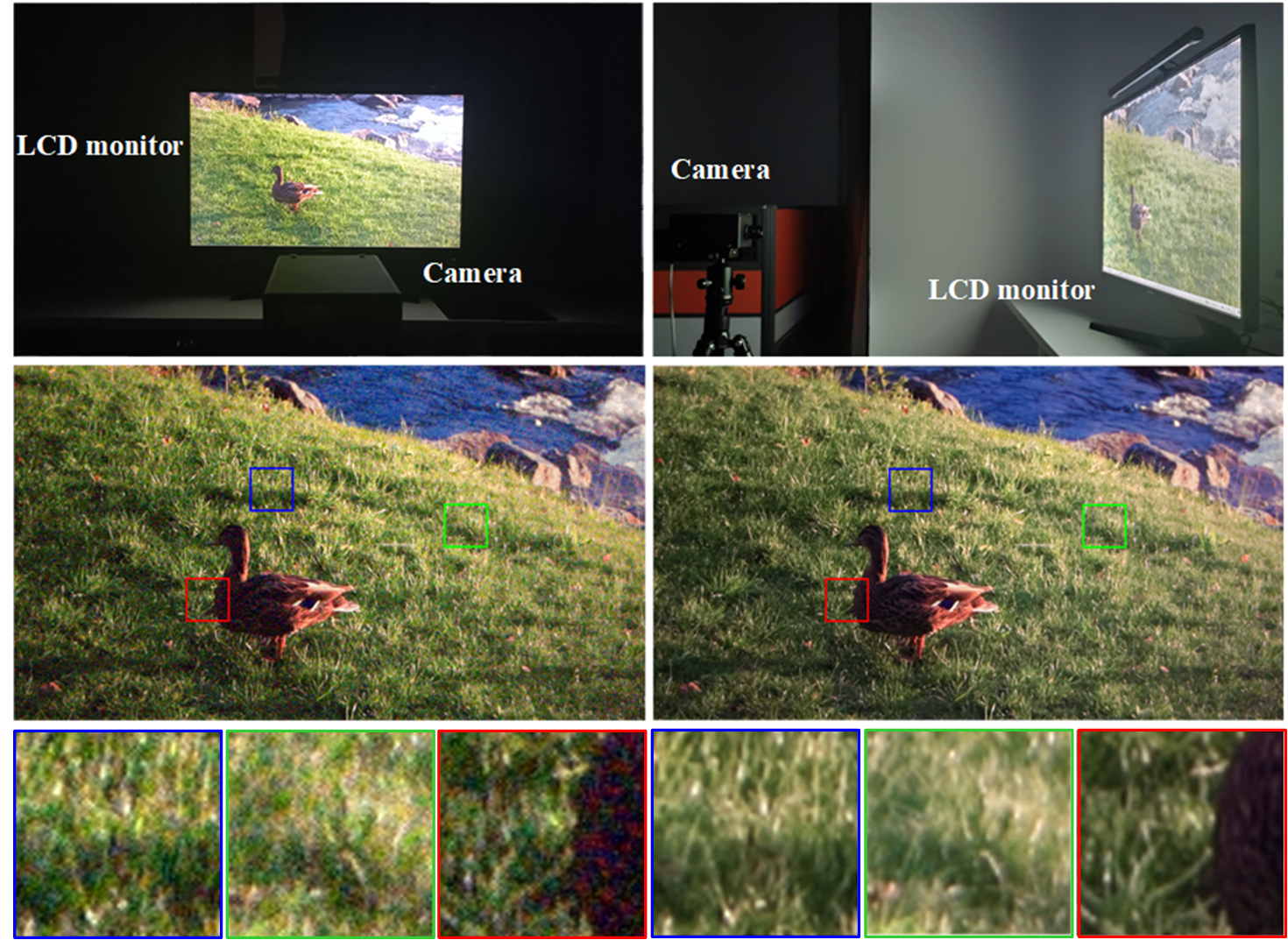
Figure 1: Illustration of our capturing system (top row), the captured noisy-clean pairs (middle row), and the close-up of three regions (bottom row).

It should be noted that recapturing the screen content may introduce unwanted moiré patterns due to the aliasing between the grids of the display screen and color filter array (CFA) in the camera sensor. Fortunately, Thongkamwitoon et al. [60] have demonstrated that such patterns can be prevented by adjusting the diaphragm aperture or focal length. In practice, we place the camera and screen as shown in Fig. 1. We maintain a constant diaphragm aperture and carefully adjust the focal length to prevent moiré patterns and lens blur in the recaptured content. Fig. 1 displays a recaptured noisy frame and its corresponding noise-free frame, along with a close-up view of the difference between the noisy and clean frames. It can be observed that the difference is pixel-independent noise without any characteristic color stripes, i.e., moiré patterns.

To eliminate the influence of ambient lighting, our dataset is captured in a darkroom. We adjust the brightness of the display screen to ensure that the luminance around the camera is low, approximately 1 lux. We captured 120 pairs of dynamic noisy-clean videos under five different ISO levels ranging from 1600 to 25600, with 24 videos captured for each ISO value. These 120 scenes are divided into a training set (90 scenes) and a testing set (30 scenes). Fig. 2 shows three frame pairs from our dataset. The sRGB frames are generated from raw inputs using our pre-trained ISP module (explained in Sec. 4.5 ). Our captured noisy-clean videos depict natural motions, since they are from real videos rather than controlled toys.

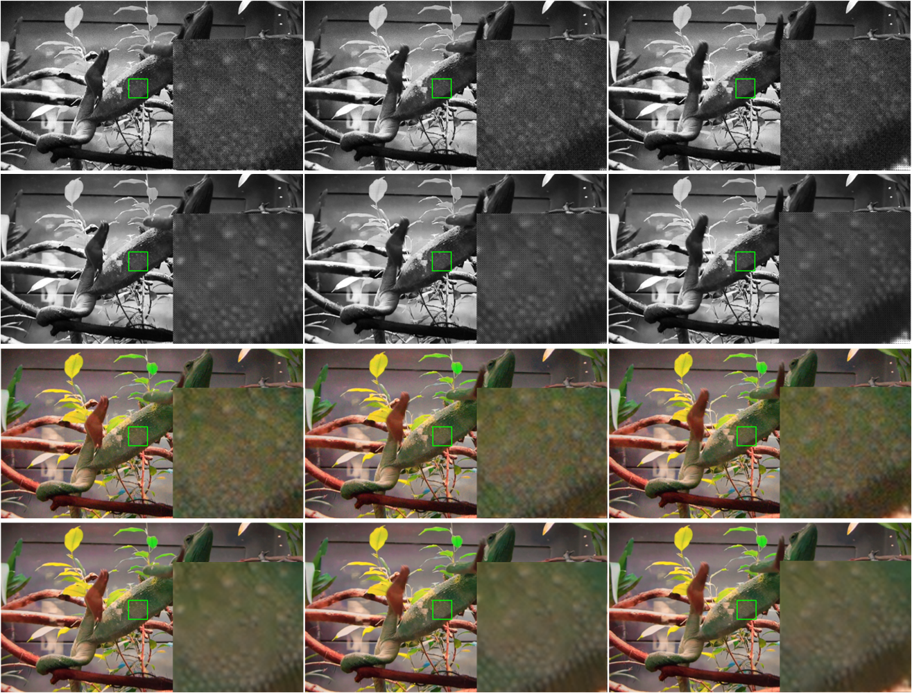
Figure 2: Sampled three frames of the captured noisy-clean video under ISO 3200. From top to down, each row lists the raw noisy video, raw clean video, sRGB noisy video, and sRGB clean video, respectively. The color videos are generated from raw video using our pre-trained ISP module.

3.2 Post Processing

There often exists brightness difference and spatial misalignment between the captured noisy frame and the corresponding clean frame due to the different ISO settings, exposure times, illuminations, and the minuscule destabilization of the camera. Therefore, we further apply post-processing to our captured data to correct brightness difference, align the clean frame to the noisy frame, and correct the color cast.

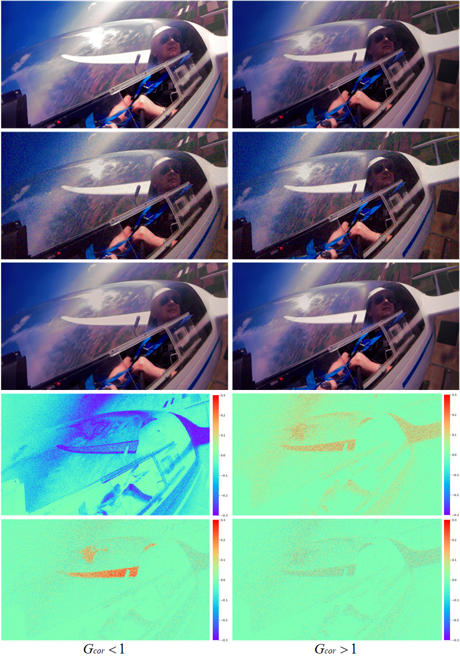
Figure 3: From top to bottom, each row lists the original clean frame, noisy frame, clean frame after intensity correction, the residual brightness channel before and after intensity correction. Left: processing with $G_{cor}<1$; Right: processing with $G_{cor}>1$ (proposed).

3.2.1 Linear Intensity Correction

We capture the displayed videos in a darkroom and keep screen luminance as a constant value so that the brightness of the captured raw frame is only influenced by ISO settings and exposure time, which can be formulated as

$$B=G\times E,$$ (1)

where $B$ is the brightness of the raw frame pixels, $G$ is the ISO gain and $E$ is the exposure time. We denote the brightness, ISO gain, exposure time for raw clean (noisy) image as $B_{c}$ ($B_{n}$), $G_{c}$ ($G_{n}$), and $E_{c}$ ($E_{n}$), respectively. In order to not change the distribution of the noise in noisy frame, we correct the clean raw frame by multiplying it with a brightness compensation coefficient $G_{cor}$ to make the clean frame have the same brightness as noisy frame. This process can be formulated as

$$B_{c}\times G_{cor}=B_{n}.$$ (2)

For a raw image, the pixel value after black level correction is linearly to $B$. In other words, the average brightness of a raw image can be estimated by averaging the pixel values. Therefore, $G_{cor}$ can be derived as follows

$$G_{cor}=\frac{B_{n}}{B_{c}}=\frac{\sum_{i,j}(I_{ij}^{n}-bl)}{\sum_{i,j}(I_{ij}^{c}-bl)}$$ (3)

where $I_{ij}^{n}$ ($I_{ij}^{c}$) denotes the pixel value of the raw noisy (clean) image at coordinates $(i,j)$, and $bl$ is the black level. Note that, the over-exposed pixel values are clipped to white level and is not linearly to $B$. When $G_{cor}$ is smaller than 1, directly applying $G_{cor}$ to $I^{c}$ will cause the over-exposed pixel values in $I^{c}$ become smaller than the white level. As shown in the left column of Fig. 3, the residual B channel (obtained by $I^{n}$-$I^{c}$ ($\hat{I}^{c}$), where $\hat{I}^{c}$ is the intensity corrected version) has large difference at the over-exposed regions, such as the person’s hat and the wings of air plane. Therefore, during capturing, we tune the exposure time and screen luminance to make the recaptured clean image a bit darker than the noisy image. In this way, the derived $G_{cor}$ is larger than 1. As shown in the right column of Fig. 3, after intensity correction, $\hat{I}^{c}$ has the same brightness as that of $I^{n}$, even in the over-exposed regions.

3.2.2 Spatial Alignment

Due to the minuscule destabilization of the camera, there are spatial misalignments between $I^{n}$ and $\hat{I}^{c}$. In this work, we utilize DeepFlow [61] to align $\hat{I}^{c}$ with $I^{n}$. Specifically, we utilize DeepFlow to compute the optical flow between Gr channel of $\hat{I}^{c}$ and $I^{n}$, and then apply the same flow to the packed four channels of $\hat{I}^{c}$ to perform the warping. In this way, the Bayer pattern of the raw image can be kept. From Fig. 4, it can be observed that there exists sharp object edge in (c) but they disappear in (d). It means that after spatial alignment, raw clean frame is well aligned to raw noisy frame. Note that, all the warping frames are carefully checked manually and the ones with alignment errors are removed away from our dataset.

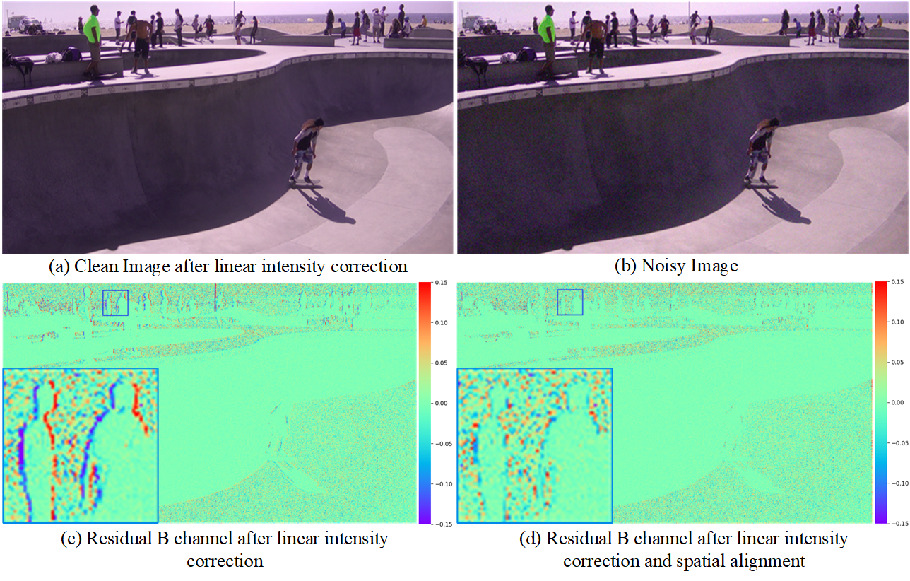
Figure 4: Differences between blue channels of noisy and clean raw frames before and after spatial alignment. Zoom in for better observation.

3.2.3 Color Correction

Due to the blue light of the electronic monitor, the images captured by the camera may have color cast, which will make the data set biased to blue tone. The color offset can be measured by the color temperature ($K_{i}$) of different channels,

$$K_{i}=\frac{\bar{C}_{R}+\bar{C}_{G_{r}}+\bar{C}_{G_{b}}+\bar{C}_{B}}{4\bar{C}_{i}},$$ (4)

where $\bar{C_{i}},i\in\left\{R,G_{r},G_{b},B\right\}$ represents the average value of channel $i$. In order to obtain the correct color temperature for each channel, we utilize [48] to convert the original RGB frame into raw frame and obtain its original color temperature $\hat{K_{i}}$. Therefore, we can obtain the correction coefficients ($\alpha_{i}$) of the blue and green channels based on the red channel by solving the following equations:

$$\frac{\bar{C}_{R}+\alpha_{G_{r}}\bar{C}_{G_{r}}+\alpha_{G_{b}}\bar{C}_{G_{b}}+\alpha_{B}\bar{C}_{B}}{4\bar{C}_{i}}=\hat{K_{i}},i\in\left\{G_{r},G_{b},B\right\}.$$ (5)

The corrected noisy frame can be obtained by $\hat{I}^{n}_{i}=\alpha_{i}I^{n}_{i}$, $i\in\left\{G_{r},G_{b},B\right\}$. The corresponding clean frame is also processed with the same $\alpha_{i}$.

In summary, after intensity correction, spatial alignment, and color correction, we obtain the paired noisy-clean frames for supervised learning. For brevity, we still utilize $I^{n}$ to denote the noisy frames in the following.

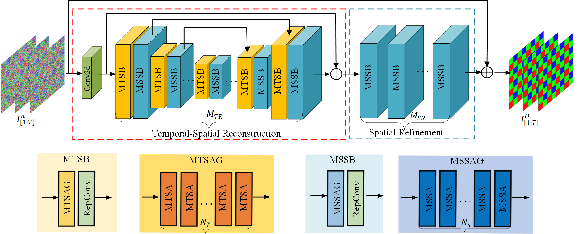
Figure 5: The framework of proposed RViDeformer, which is constructed by temporal-spatial reconstruction (containing $M_{TR}$ blocks) and spatial refinement (containing $M_{SR}$ blocks) modules.

4 The Proposed RViDeformer

In this section, we first introduce the network structure of our proposed raw video denoising transformer (RViDeformer), and then present its key components, i.e., the multi-branch spatial self-attention block (MSSB) and temporal self-attention block (MTSB).

4.1 Network Structure Overview

Given a set of consecutive Bayer raw noisy frames $I^{n}_{[1:T]}$, we aim to recover the raw clean frames $I^{GT}_{[1:T]}$ through our network RViDeformer, as illustrated in Fig. 5. The noisy sequence $I^{n}_{[1:T]}$ is first packed into four channels, and goes through the MTSB and MSSB block alternatively to exploit temporal-spatial correlations. After temporal-spatial reconstruction, the features are fed into the spatial refinement module to generate the denoised raw frames $I^{O}_{[1:T]}$, which are then transformed to sRGB domain via a pre-trained ISP module. There are $M_{TR}$ blocks in the temporal-spatial reconstruction module and $M_{SR}$ blocks in the spatial refinement module. The crucial components of our network are the MSSB and MTSB blocks, which are described in detail in the following.

4.2 Multi-Branch Spatial Self-Attention (MSSA)

The recent transformer-based video denoising methods [9, 10, 11] are all based on Swin Transformer [15, 16], which divides images with non-overlapping windows and only apply self-attention inside the window. Although Swin Transformer tries to exchange the information between windows through window shift operation, but the exchanged areas are limited and the long-range information can not be utilized. To solve this problem, we propose Global-Window and Neighbour-Window Self-Attention to enable exploring correlation from global and the neighbor areas. Since the downsampling operation can reduce noise but preserve the low frequency information, we further propose Low-Resolution Self-Attention to make each window not only learn from itself but also from its downsampled version. Afterward, we combine the multiple self-attention branches via feature fusion.

We would like to point out that multi-branch structure has been applied to build transformer in classification [62, 63] and image super-resolution [64]. Among them, [62] utilizes dual branch to combine image tokens of different sizes, [63] designs two parallel branch to combine MobileNet and transformer, and [64] constructs a multi-branch structure where different branches utilize different window size for self-attention. In contrast, we utilize the same window size for the Queries but utilize different window sizes for Keys and Values. In this way, we can utilize correlated information from different receptive fields for video denoising.

4.2.1 Shift-Window Self-Attention (SWSA)

The SWSA is the same as that defined in SwinIR [16]. Given a noisy frame feature $F\in\mathbb{R}^{H\times W\times C}$, we split it into $\lfloor\frac{H}{h}\rfloor\times\lfloor\frac{W}{w}\rfloor$ windows, where the window size is h$\times$w. For the $i$-th window $F_{i}\in\mathbb{R}^{N\times C}$ (where $N=hw$), we project it into query $Q_{i}$, key $K_{i}$, and value $V_{i}$ by linear projection,

$$Q_{i}=F_{i}P^{Q},\quad K_{i}=F_{i}P^{K},\quad V_{i}=F_{i}P^{V},$$ (6)

where $P^{Q},P^{K},P^{V}\in\mathbb{R}^{C\times D}$ are projection matrices and $D$ is the channel number of projected features. We use $Q_{i}$ to query $K_{i}$ in order to generate the attention map $A_{i}=\text{SoftMax}(Q_{i}(K_{i})^{T}/\sqrt{D})\in\mathbb{R}^{N\times N}$, and $A_{i}$ is used for weighted sum of $V_{i}$, namely $\text{SWSA}(Q_{i},K_{i},V_{i})=A_{i}V_{i}$. The SoftMax denotes the row softmax operation. In this way, we generate the enhanced feature $F^{o}_{i}\in\mathbb{R}^{N\times D}$, whose noise is reduced through the weighted average of similar features inside the window itself.

4.2.2 Global-Window Self-Attention (GWSA)

In SWSA, we utilize the same window to generate the query, key, and value of the transformer. However, this approach limits the calculation of correlations to only occur within the window. For GWSA, we propose to down sample the whole feature map $F\in\mathbb{R}^{H\times W\times C}$ to the window size to construct a global window $F^{g}\in\mathbb{R}^{N\times C}$. For the $i$-th window, the queries are obtained by linear projection of $F_{i}$ (as defined in SWSA), while the keys and values are obtained by linear projection of $F^{g}$. Namely

$$Q^{g}_{i}=F_{i}P^{Q}_{g},\quad K^{g}=F^{g}P^{K}_{g},\quad V^{g}=F^{g}P^{V}_{g},$$ (7)

where $P^{Q}_{g},P^{K}_{g},P^{V}_{g}\in\mathbb{R}^{C\times D^{g}}$ are projection matrices and $D^{g}$ is the channel number of projected features. Afterwards, we generate the attention map $A^{g}_{i}=\text{SoftMax}(Q^{g}_{i}(K^{g})^{T}/\sqrt{D^{g}})\in\mathbb{R}^{N\times N}$ to fuse the values $V^{g}$, resulting in $F^{og}_{i}\in\mathbb{R}^{N\times D^{g}}$. In this way, the feature of each local window is predicted by the fusion of global downsampled features.

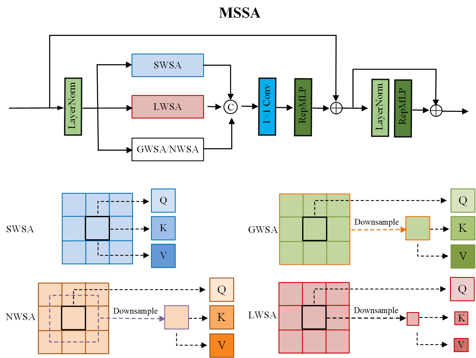
Figure 6: The framework of proposed MSSA.

4.2.3 Neighbour-Window Self-Attention (NWSA)

When the window number $\lfloor\frac{H}{h}\rfloor\times\lfloor\frac{W}{w}\rfloor$ is large, the global window $F^{g}$ cannot represent the detailed features. Therefore, we further propose Neighbour-Window Self-Attention (NWSA), which utilizes the information from a large neighbour area rather than the global feature map. As shown in Fig. 6, for the $i$-th window $F_{i}$, we downsample its neighbour area to make the large neighbor have the same size as $F_{i}$, generating a neighbour-window $F^{n}_{i}\in\mathbb{R}^{h\times w\times C}$, reshaped as $F^{n}_{i}\in\mathbb{R}^{N\times C}$. Then we compute the query $Q^{n}_{i}$, key $K^{n}_{i}$ and value $V^{n}_{i}$ from $F_{i}$ and $F^{n}_{i}$ by linear projections as

$$Q^{n}_{i}=F_{i}P^{Q}_{n},\quad K^{n}_{i}=F^{n}_{i}P^{K}_{n},\quad V^{n}_{i}=F^{n}_{i}P^{V}_{n},$$ (8)

where $P^{Q}_{n},P^{K}_{n},P^{V}_{n}\in\mathbb{R}^{C\times D^{n}}$ are projection matrices and $D^{n}$ is the channel number of projected features. We use $Q^{n}_{i}$ to query $K^{n}_{i}$ to generate the attention map $A^{n}_{i}=\text{SoftMax}(Q^{n}_{i}(K^{n}_{i})^{T}/\sqrt{D^{n}})\in\mathbb{R}^{N\times N}$, and $A^{n}_{i}$ is used for weighted sum of $V^{n}_{i}$, generating the enhanced feature $F^{on}_{i}\in\mathbb{R}^{N\times D^{n}}$. In other words, the feature of each local window is predicted by the feature in down-sampled neighbor window.

4.2.4 Low-Resolution-Window Self-Attention (LWSA)

Multi-scale architecture is beneficial for denoising. In RViDeformer, we not only utilize it in constructing the UNet-like backbone, but also apply it in the transformer structure, namely the values of the transformer are from windows with different receptive fields. For GWSA and NWSA, we are actually utilizing the information from large areas. Therefore, we further propose to utilize the information from the window itself but in a low-resolution version. For the $i$-th window $F_{i}$, we downsample it with scale $2$ to construct a lower resolution window $F^{l}_{i}\in\mathbb{R}^{\frac{N}{4}\times C}$. $F^{l}_{i}$ reduces the noise in $F_{i}$ but still preserves the structure of input image. Then, the query $Q^{l}_{i}$, key $K^{l}_{i}$ and value $V^{l}_{i}$ are derived by

$$Q^{l}_{i}=F_{i}P^{Q}_{l},\quad K^{l}_{i}=F^{l}_{i}P^{K}_{l},\quad V^{l}_{i}=F^{l}_{i}P^{V}_{l},$$ (9)

where $P^{Q}_{l},P^{K}_{l},P^{V}_{l}\in\mathbb{R}^{C\times D^{l}}$ are projection matrices and $D^{l}$ is the channel number of projected features. Then we calculate the attention weights $A^{l}_{i}=\text{SoftMax}(Q^{l}_{i}(K^{l}_{i})^{T}/\sqrt{D^{l}})\in\mathbb{R}^{N\times\frac{N}{4}}$ to fuse $V^{l}_{i}$, generating $F^{ol}_{i}\in\mathbb{R}^{N\times D^{l}}$.

As shown in Fig. 6, we construct three self-attention branches, namely SWSA, LWSA, and GWSA (or NWSA) respectively. Specifically, we apply NWSA for the MSSB and MTSB blocks in the original resolution and GWSA is applied on the other blocks since applying GWSA on the original resolution will lose much information. Since the proposed GWSA, NWSA, and LWSA are also window based, we utilize the shift window operation on them for better performance. Finally, we fuse the three outputs $F^{o}_{i},F^{ol}_{i},F^{on}_{i}(F^{og}_{i})$ via a 1$\times$1 convolution layer and adjust the contributions of each branch by the parameters $D$, $D^{l}$ and $D^{n}$ ($D^{g}$). We utilize $N_{S}$ MSSA to construct one MSSA Group (MSSAG).

4.3 Multi-Branch Temporal Mutual Self-Attention (MTSA)

VRT [10] proposes Temporal Mutual Self-Attention to exploit temporal information from neighbour frames, but the self-attention operation is limited inside the window, which can not process large movements. Therefore, they further introduce warping module to align the neighbor frames (i.e., supporting frames) with the reference frame. Different from it, we propose to utilize transformer to perform implicit alignment by adjusting the window region of the supporting frames. Similar to our proposed MSSA block, we further propose Multi-branch Temporal Mutual Self-Attention (MTSA), which utilizes the Global-Window and Neighbour-Window Self-Attention to process the movements between the reference and supporting frames, as shown in Fig. 7.

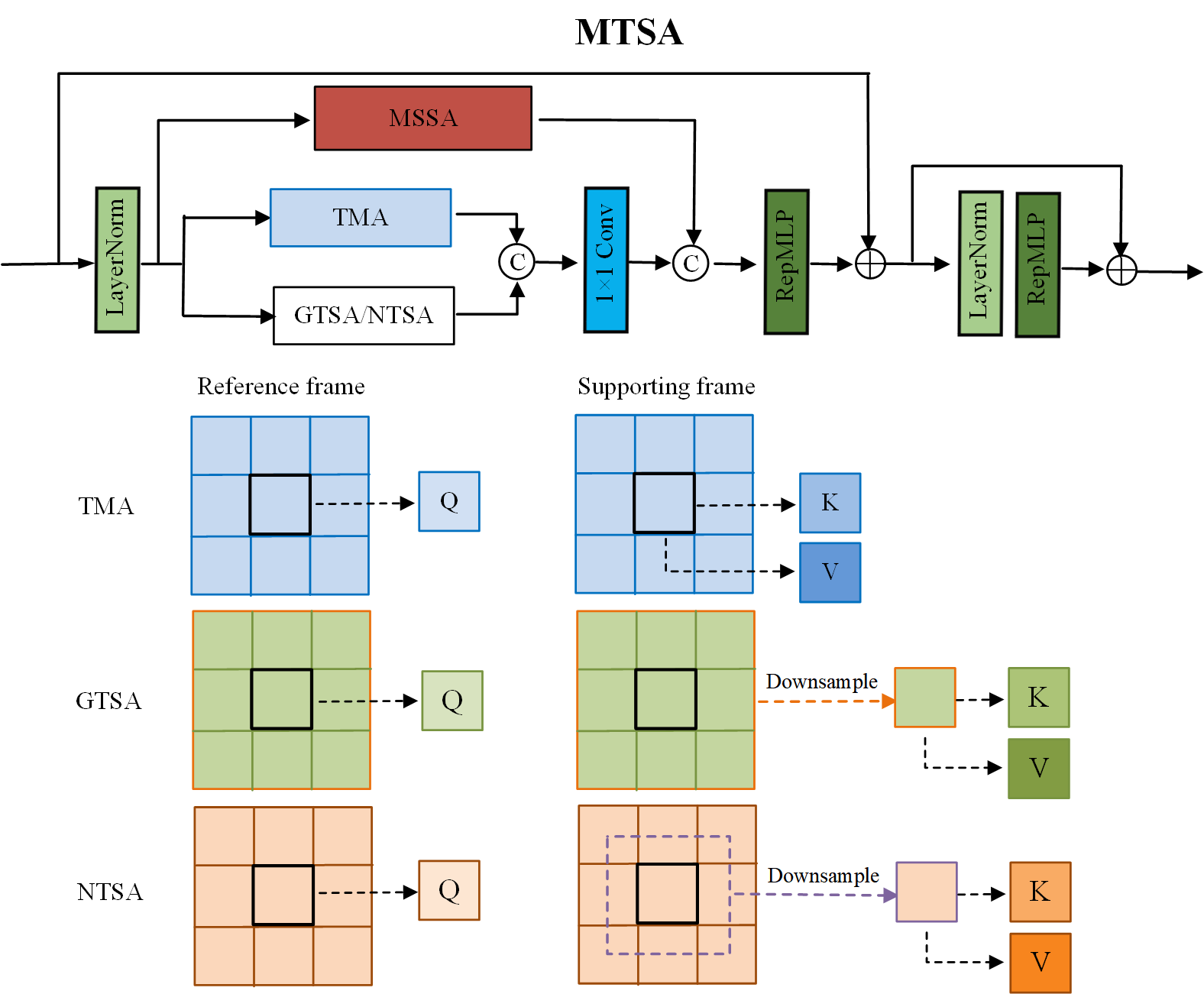
Figure 7: The framework of proposed MTSA.

Given a reference frame feature $F^{R}\in\mathbb{R}^{H\times W\times C}$ and a supporting frame feature $F^{S}\in\mathbb{R}^{H\times W\times C}$, we first split them into windows. For the reference frame, we split it into $\lfloor\frac{H}{h}\rfloor\times\lfloor\frac{W}{w}\rfloor$ windows, where the window size is h$\times$w, and the $i$-th window can be denoted as $F^{R}_{i}\in\mathbb{R}^{h\times w\times C}$. For the supporting frame, we split it into windows in three ways. The first is the same as that in reference frame, namely the $i$-th window is $F^{S}_{i}\in\mathbb{R}^{h\times w\times C}$. The second is global-window, namely we directly down-sample the whole feature map to the window size, constructing the global window $F^{Sg}\in\mathbb{R}^{h\times w\times C}$. The third is neighbor window, namely we downsample a large neighbor region centered at the $i$-th window into $F^{Sn}_{i}\in\mathbb{R}^{h\times w\times C}$. According to different window settings in the supporting frame, we construct three different temporal self-attention mechanisms, i.e., the plain Temporal Mutual Attention (TMA), Global-Window Temporal Mutual Attention (GTMA), and Neighbour-Window Temporal Mutual Attention (NTMA). Specifically, the query, key, and value for the three attentions are denoted as

$$\begin{split}&\text{TMA:}\;Q^{R}_{i}=F^{R}_{i}P^{Q}_{R},\;K^{S}_{i}=F^{S}_{i}P^{K}_{S},\;V^{S}_{i}=F^{S}_{i}P^{V}_{S}\\ &\text{GTSA:}\;Q^{Rg}_{i}=F^{R}_{i}P^{Q}_{Rg},\;K^{Sg}=F^{Sg}P^{K}_{Sg},\;V^{Sg}=F^{Sg}P^{V}_{Sg}\\ &\text{NTSA:}\;Q^{Rn}_{i}=F^{R}_{i}P^{Q}_{Rn},\;K^{Sn}_{i}=F^{Sn}_{i}P^{K}_{Sn},\;V^{Sn}_{i}=F^{Sn}_{i}P^{V}_{Sn},\\ \end{split}$$ (10)

where $P^{Q}_{R},P^{K}_{S},P^{V}_{S}\in\mathbb{R}^{C\times D_{T}}$ , $P^{Q}_{Rg},P^{K}_{Sg},P^{V}_{Sg}\in\mathbb{R}^{C\times D^{g}_{T}}$ and $P^{Q}_{Rn},P^{K}_{Sn},P^{V}_{Sn}\in\mathbb{R}^{C\times D^{n}_{T}}$ are projection matrices. Note that all the features are reshaped into $N\times C$ before the projection operation. Then, we calculate the attention coefficients between the query and corresponding key, and then generate the fusion result by weighted average of the corresponding values based on the attention coefficients, similar to that in MSSA.

As shown in Fig. 7, we construct the first branch of MTSA with TMA, and construct the second branch with GTMA (NTMA). Similar to MSSA, NTMA is applied on the blocks with original resolution and GTMA is applied on the other blocks with low resolution. Through our proposed GTMA and NTMA, RViDeformer can utilize the information with large movements from the supporting frames. Note that, we also introduce the MSSA module during temporal reconstruction to further enhance the spatial correlations. We utilize $N_{T}$ MTSA to construct one MTSA Group (MTSAG).

4.4 Reparameterization

Reparameterized MLP (RepMLP). For transformer, we usually utilize MLP after the self-attention layers. In this work, we propose to utilize two MLPs during training to increase the capability of the network. During test, we utilize reparameterization to fuse the two linear layers into one linear layer. In this way, the inference cost is the same as that for one MLP layer, as shown in Fig. 8. Specifically, during training, the $C_{in}$-channel feature map $I\in\mathbb{R}^{C_{in}\times H\times W}$ goes through two parallel linear layers with weights $W_{L1},W_{L2}\in\mathbb{R}^{C_{out}\times C_{in}}$ and bias $b_{L1},b_{L2}\in\mathbb{R}^{D}$, generating the corresponding $C_{out}$-channel feature maps $O_{L1}$ and $O_{L2}\in\mathbb{R}^{C_{out}\times H\times W}$, respectively. $O_{L1}$ and $O_{L2}$ are then added together and activated by GELU layer, then goes through a dropout and a linear layer to generate the final result. When inference, based on the linearity of the linear layer, two parallel linear layers can be fused into one linear layer with weights $W_{Lf}$ and $b_{Lf}$, which can be formulated as

$$\begin{split}W_{Lf}&=W_{L1}+W_{L2},\\ b_{Lf}&=b_{L1}+b_{L2}.\\ \end{split}$$ (11)

Reparameterized Convolution (RepConv). In the end of each MTSB (MSSB), we further utilize a 3$\times$3 2D convolution to model the local spatial context. Therefore, the last linear layer (which is equal to a 1$\times$1 2D convolution) in the transformer (MTSAG or MSSAG) can be fused with the convolution layer during inference. The weights of two convolutions before fusion can be denoted as $W_{C1}\in\mathbb{R}^{C_{out}\times C_{in}\times 1\times 1}$, $W_{C2}\in\mathbb{R}^{C_{out}\times C_{in}\times 3\times 3}$. Similarly, the bias can be denoted as $b_{C1},b_{C2}\in\mathbb{R}^{D}$. The weight and bias of fused convolution can be denoted as $W_{Cf}\in\mathbb{R}^{C_{out}\times C_{in}\times 3\times 3}$ and $b_{Cf}\in\mathbb{R}^{D}$. According to [65], the fused convolution parameters are

$$\begin{split}W_{Cf}&=\text{conv}(W_{C2},W^{T}_{C1}),\\ b_{Cf}&=\text{sum}(W_{C2}b_{C1})+b_{C2}.\\ \end{split}$$ (12)

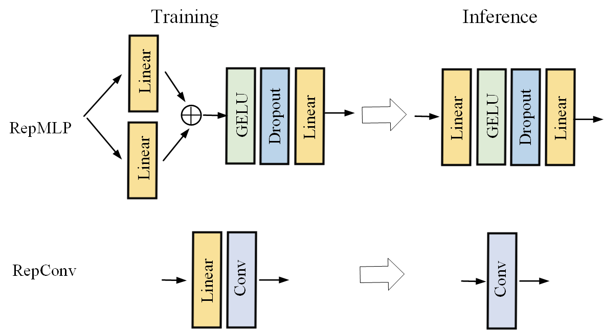
Figure 8: The architectures of RepMLP and RepConv.

4.5 ISP

We utilize the ISP module proposed by [12] to transfer raw denoising results $I^{O}_{[1:T]}$ to the sRGB domain $S^{O}_{[1:T]}$. The ISP module has a UNet architecture, which is trained with 230 clean raw and sRGB pairs from SID dataset [41]. By changing the training pairs, we can simulate ISPs of different cameras. In addition, ISP module can also be replaced by traditional ISP pipelines [49].

4.6 Loss Functions

In this work, we adopt two kinds of loss functions, which are used for supervised and unsupervised video denoising tasks, respectively.

Supervised loss. Our supervised loss function includes raw and sRGB domain reconstruction losses, which can be formulated as

$$\begin{split}\mathcal{L}_{\text{raw}}=&\|I^{O}_{t}-I^{GT}_{t}\|_{1}\\ \mathcal{L}_{\text{sRGB}}=&\|S^{O}_{t}-S^{GT}_{t}\|_{1}\\ \mathcal{L}_{\text{sup}}=&\mathcal{L}_{\text{raw}}+\beta_{1}\mathcal{L}_{\text{sRGB}}\\ \end{split}$$ (13)

where $I^{O}_{t}$ and $S^{O}_{t}$ denote the raw and sRGB output of the network for the $t$-th frame, $I^{GT}_{t}$ and $S^{GT}_{t}$ denote the corresponding ground truths. The parameters of the pretrained ISP are fixed when training the denoising network, which is beneficial for improving the reconstruction quality in the sRGB domain. $\beta_{1}$ is the hyper-parameter to balance the two losses.

Unsupervised loss. For unsupervised video denoising, the key is to build noisy-noisy pairs for Noise2Noise training [1] from video data. F2F [4] and MF2F [5] utilize neighboring frames after warping for Noise2Noise training, where the warping error negatively impact the performance. Therefore we construct noisy-noisy pairs only from single frame. In this work, we utilize the NBR2NBR loss [17]. Specifically, for the $t$-th noisy frame $I^{n}_{t}$, we sub-sample it with a neighbor down-sampler to get sub-frames $I^{ns1}_{t}$ and $I^{ns2}_{t}$. We feed the network with $I^{ns1}_{t}$ to generate the denoising result $I^{sO1}_{t}$. Then, with $I^{n}_{t}$ as input, we get $I^{O}_{t}$ and downsample $I^{O}_{t}$ with the same neighbor down-sampler to get sub-frames $I^{Os1}_{t}$ and $I^{Os2}_{t}$. The spatial NBR2NBR loss can be formulated as

$$\begin{split}\mathcal{L}_{\text{rec}}=&\|I^{sO1}_{t}-I^{ns2}_{t}\|^{2}_{2}\\ \mathcal{L}_{\text{reg}}=&\|I^{sO1}_{t}-I^{ns2}_{t}-(I^{Os1}_{t}-I^{Os2}_{t})\|^{2}_{2}\\ \mathcal{L}_{\text{unsup}}=&\mathcal{L}_{\text{rec}}+\beta_{2}\mathcal{L}_{\text{reg}},\\ \end{split}$$ (14)

where $\beta_{2}$ is the hyper-parameter controlling the strength of the $\mathcal{L}_{\text{reg}}$.

5 Experiments

5.1 Implementation Details

For a fair comparison with other video denoising methods under similar computation cost, we build four different versions of RViDeformer as shown in Table I: RViDeformer-T (Tiny), RViDeformer-S (Small), RViDeformer-M (Medium), and RViDeformer-L (Large). They are designed by changing the base channel number of projected features in MTSA and MSSA (i.e. $D_{T}$ in Eq. 10 and $D$ in Eq. 6), the block number in temporal-spatial reconstruction and spatial refinement modules (i.e., $M_{TR}$ and $M_{SR}$), and the number of self-attention block in MTSAG and MSSAG (i.e., $N_{T}$ and $N_{S}$). For all the four versions, the head number in multi-head self-attention is set to 6. The channel numbers of projected features in LWSA ($D^{l}$), GWSA ($D^{g}$), and NWSA ($D^{n}$) branches are half of that ($D$) in SWSA branch of MSSA block, respectively. The channel numbers of projected features in GTMA ($D^{g}_{T}$) and NTMA ($D^{l}_{T}$) branches are half of that ($D_{T}$) in TMA branch of MTSA block, respectively.

Since LLRVD [14] has not released their dataset, we compare our method with state-of-the-art raw video denoising methods on our proposed ReCRVD dataset and CRVD dataset [12]. For supervised and unsupervised video denoising on ReCRVD dataset, we train our network with 12000 epochs, and the learning rate starts with 1e-4 and drops to 5e-5 and 2e-5 after 2/6 and 5/6 of total epochs. For supervised and unsupervised video denoising on CRVD dataset, we train our network with 30000 epochs, and the learning rate starts with 1e-4 and drops to 5e-5 and 2e-5 after 4/6 and 5/6 of total epochs. The hyper-parameter $\beta_{1}$ in supervised loss is set to 0.5, and the hyper-parameter $\beta_{2}$ in unsupervised loss is set to 2$\times$(epoch/(total epoch)). The batch size and patch size are set to 1 and 64, respectively. The temporal number $T$ is set to 6 during training. The experiments are conducted with an NVIDIA 3090 GPU.

TABLE I: Detailed configurations of different versions of our RViDeformer. The MACs are calculated based on the Bayer raw input with a resolution of 1920$\times$1080.

Models	$D_{T}$	$D$	$M_{TR}$	$M_{SR}$	$N_{T}$	$N_{S}$	heads	GMACs
RViDeformer-T	24	24	14	2	1	1	6	38.81
RViDeformer-S	24	30	14	3	2	1	6	71.30
RViDeformer-M	24	30	14	4	4	2	6	143.67
RViDeformer-L	84	108	14	4	4	2	6	1790.86

5.2 Comparison with State-of-the-art Methods

TABLE II: Quantitative comparisons of PSNR and SSIM for supervised raw video denoising on the ReCRVD test set. The GMACs for one frame are calculated based on the Bayer raw input with a resolution of 1920$\times$1080.

Methods	GMACs	raw	sRGB
VBM4D [24]	-	39.68/0.9475	33.65/0.8962
FastDVDnet [7]	332.23	43.49/0.9806	38.87/0.9615
EMVD∗ [27]	177.82	43.32/0.9794	38.60/0.9587
BSVD-32 [28]	153.65	43.56/0.9807	39.06/0.9619
RViDeformer-M	143.67	43.98/0.9823	39.57/0.9652
RViDeNet [12]	2079.74	43.71/0.9811	39.09/0.9627
FloRNN [8]	2316.73	44.01/0.9829	39.42/0.9672
RVRT∗ [11]	3152.25	43.97/0.9821	39.43/0.9648
VRT∗ [10]	3056.48	44.07/0.9826	39.69/0.9662
RViDeformer-L	1790.86	44.37/0.9837	40.15/0.9695

TABLE III: Quantitative comparisons of PSNR and SSIM for supervised raw video denoising on the CRVD test set. The GMACs for one frame are calculated based on the Bayer raw input with a resolution of 1920$\times$1080. The results of VBM4D are quoted from [12]. The results of EDVR and FastDVDnet are quoted from [27]. The results of FastDVDnet-S are quoted from [66].

Methods	GMACs	raw	sRGB
VBM4D [24]	-	-	34.16/0.9220
EMVD [27]	39.76	44.05/0.9890	39.53/0.9796
BSVD-16 [28]	39.38	44.10/0.9884	40.17/0.9804
RViDeformer-T	38.81	44.34/0.9887	40.60/0.9813
FastDVDnet-S [7]	146.99	44.25/0.9887	-
BSVD-24 [28]	87.73	44.39/0.9894	40.48/0.9820
BP-EVD [66]	72.39	44.42/0.9889	-
RViDeformer-S	71.30	44.65/0.9894	41.00/0.9828
LLRVD [14]	1724.52	44.18/0.9880	-
EDVR [67]	1544.49	44.71/0.9902	40.89/0.9838
EMVD-L [27]	1272.75	44.58/0.9899	-
FastDVDnet [7]	332.50	44.30/0.9891	39.91/0.9812
RViDeformer-M	143.67	44.89/0.9901	41.29/0.9840
RViDeNet [12]	2079.74	43.97/0.9874	39.95/0.9792
FloRNN [8]	2316.73	45.16/0.9907	41.01/0.9843
RViDeformer-L	1790.86	45.45/0.9913	41.86/0.9860

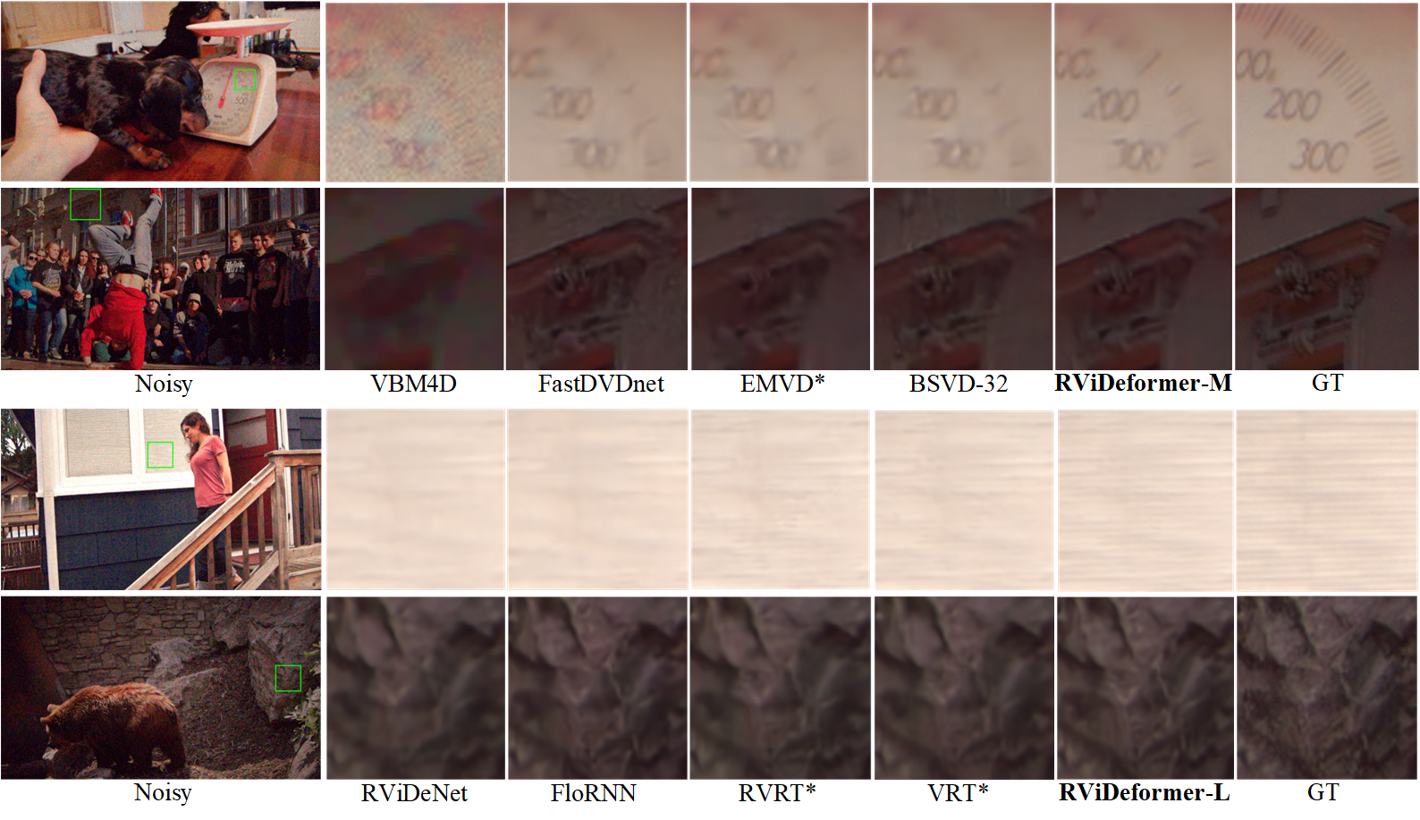
Figure 9: Visual quality comparison on ReCRVD test set for supervised raw video denoising. Zoom in for better observation.

To demonstrate the effectiveness of the proposed raw video denoising methods, we compare with state-of-the-art video denoising methods for supervised learning and unsupervised learning, respectively.

Supervised learning on ReCRVD dataset. For supervised learning, we compare our method with eight video denoising methods, i.e., VBM4D [24], FastDVDnet [7], RViDeNet [12], EMVD [27], BSVD [28], FloRNN [8], RVRT [11], and VRT [10]. For a fair comparison, all the methods are retrained on the training set of ReCRVD. Due to the significant variation in computation costs among these video denoising methods, we categorize them into two groups based on their computation costs. The first group is constructed by lightweight video denoising methods (FastDVDnet, EMVD, BSVD-32) and the traditional denoising method VBM4D. Among them, BSVD-32 is a lighter version of BSVD. Since the code of EMVD has not been released, we use an unofficial implementation , and we denote it as EMVD^∗. For VBM4D, we observe that processing in raw domain can achieve better results. Therefore, we pack the Bayer raw input into 4 channels and process each channel with VBM4D separately. We compare these light-weight video denoising methods with RViDeformer-M, which is a lighter version of our network. The second group contains large video denoising models (RViDeNet, FloRNN, RVRT, VRT) with more computation costs, and we compare them with our RViDeformer-L. Since the optical flow network in VRT and RVRT can only process 3-channel RGB inputs and can not process raw data, we apply a simple ISP to the raw inputs before feeding them to the optical flow network. To unify the computation cost of the second group to a similar level, we reduce the base channel number and the depths of VRT for a fair comparison, which is denoted as VRT^∗. For the same reason, we reduce the base channel number of RVRT, which is denoted as RVRT^∗. We evaluate these methods on the test set of proposed ReCRVD dataset.

Table II lists the average PSNR and SSIM values of raw video denoising results in raw and sRGB domains on ReCRVD test set, which contains 30 videos and each video contains 25 frames. It can be observed that our model greatly outperforms the state-of-the-art small and large video denoising models. For lighter video denoising methods, RViDeformer-M outperforms the second best method BSVD-32 by 0.42 (0.51) dB in raw (sRGB) domain. For heavier video denoising methods, RViDeformer-L outperforms the second best method VRT^∗ 0.30 (0.46) dB in raw (sRGB) domain. In addition, our model consumes the lowest MACs (multiply-add operations). Fig. 9 presents the visual comparison results on four scenes of ReCRVD test set. It can be observed that our method can remove the noise clearly and recover the most details. VBM4D either cannot remove the noise (such as the first scene) or generate over-smooth results (such as the second scene). The results of light-weight methods, i.e., FastDVDnet, EMVD* and BSVD-32 are a bit smooth in the first scene, and contain artifacts in the second scene. Compared with computational heavy methods, our method recovers more details, as shown in the third and fourth scenes of Fig. 9.

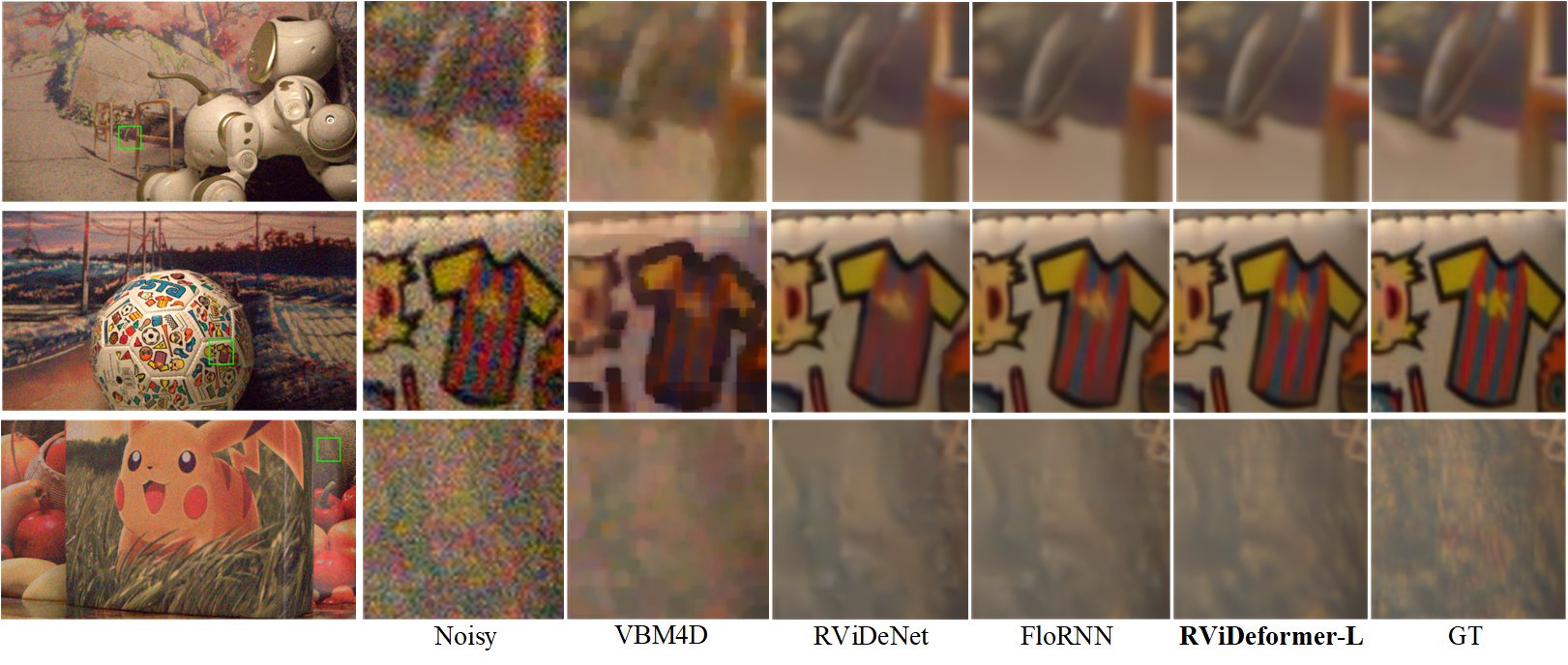
Figure 10: Visual quality comparison on CRVD test set for supervised raw video denoising. Zoom in for better observation.

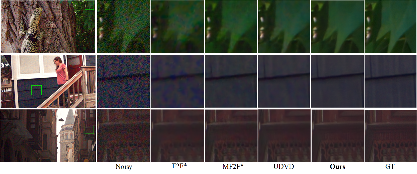
Figure 11: Visual quality comparison on ReCRVD test set for unsupervised raw video denoising. Zoom in for better observation.

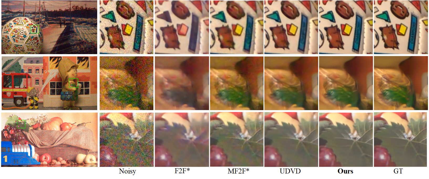
Figure 12: Visual quality comparison on CRVD indoor test set for unsupervised raw video denoising. Zoom in for better observation.

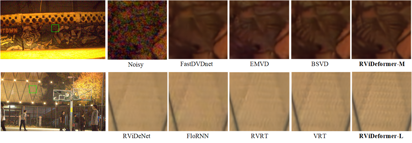
Figure 13: Visual quality comparison on CRVD outdoor test set for supervised raw video denoising methods trained on ReCRVD dataset. Zoom in for better observation.

Supervised learning on CRVD indoor dataset. We also give the comparison results on CRVD indoor dataset [12]. CRVD indoor dataset is a popular benchmark dataset for raw video denoising, which contains 55 videos among which 6 scenes are used for training and the other 5 scenes are used for testing. Most of the above mentioned methods have been evaluated on this dataset. Therefore, we directly quote their scores from their papers. We further introduce BP-EVD [66] and LLRVD [14] for comparison. Since they are not open-sourced, we did not compare them on ReCRVD dataset. Since we have compared with RVRT and VRT on ReCRVD dataset, we do not retrain and compare them on CRVD dataset. For the methods with light-weight models, we compare these methods with RViDeformer-S or RViDeformer-T. In summary, we categorize these methods into four groups and the methods in each group have similar computation costs.

Table III lists the average PSNR and SSIM values of raw video denoising results in raw and sRGB domains on CRVD test set. It can be observed that our models greatly outperform the SOTA video denoising methods in each group. For the first group, RViDeformer-T outperforms the second best method BSVD-16 by 0.24 (0.43) dB in raw (sRGB) domain. For the second group, RViDeformer-S outperforms the second best method BP-EVD by 0.23 dB in raw domain. For the third group, RViDeformer-M outperforms the second best method FastDVDnet by 0.59 (1.38) dB in raw (sRGB) domain. For the fourth group, RViDeformer-L outperforms the second best method FloRNN by 0.29 (0.85) dB in raw (sRGB) domain. For each group, our method has the lowest MACs. Fig. 10 presents the visual comparison results on three scenes of CRVD indoor test set. Since only RViDeNet and FloRNN have released their models, we only compare them and VBM4D on CRVD dataset. It can be observed that our method recovers the most details in all three scenes.

Unsupervised learning on ReCRVD dataset. For unsupervised learning, we compare our method with state-of-the-art unsupervised video denoising methods F2F [4], MF2F [5], and UDVD [6]. All methods are retrained on the training set of ReCRVD dataset without utilizing the ground truths. F2F and MF2F utilize DnCNN [18] and FastDVDNet as their denoising network, respectively. We utilize RViDeformer-L as our denoising network. For a fair comparison, we increase the channel number of DnCNN [18] and FastDVDnet to unify the computation cost of them to be similar to that of our method, and we denote them as F2F^∗ and MF2F^∗, respectively. We evaluate all the methods on the test set of ReCRVD dataset. Table IV lists the average PSNR and SSIM values of unsupervised raw video denoising results on ReCRVD test set in both raw and sRGB domains. It can be observed that our model outperforms the SOTA unsupervised video denoising methods. Compared with the second best method UDVD, our method achieves 0.02 (1.11) dB gain in raw (sRGB) domain and much higher SSIM values. The main reason is that UDVD tends to generate smooth results in raw domain (which leads to good PSNR result but worse SSIM value in raw domain) and its sRGB domain results contain many artifacts (which leads to worse PSNR values in sRGB domain). Our method also has the lowest MACs. It proves that our proposed network RViDeformer is also a good architecture for unsupervised video denoising. Fig. 11 presents the visual comparison results on the ReCRVD test set for unsupervised raw video denoising. It can be observed that the results of compared three unsupervised methods contains much chroma noise. The results of F2F* and MF2F* contain some artifacts. Meanwhile, the results of F2F* and UDVD are over-smooth in the third scene. In contrast, our method removes the noise clearly and recover the most details.

Unsupervised learning on CRVD indoor dataset. We also give the comparison results of unsupervised video denoising methods on CRVD indoor dataset. We retrain the above three unsupervised methods on the training set and evaluate them on the test set of CRVD. In UDVD [6], its results are generated by training and testing on the same scenes of CRVD test set. Since it is inconsistent with the real world case, we retrain UDVD on the training set and evaluate it with the test set. Table V lists the average PSNR and SSIM values of unsupervised raw video denoising results on CRVD test set. It can be observed that our model outperforms the second best method UDVD with 1.56 dB gain in sRGB domain. Fig. 12 presents the visual comparison results on the CRVD indoor test set. It can be observed that our method removes the noise clearly and recovers the most details in all three scenes.

TABLE IV: Quantitative comparisons of PSNR and SSIM for unsupervised raw video denoising on ReCRVD test set. The GMACs for one frame are calculated based on the Bayer raw input with a resolution of 1920$\times$1080.

Methods	GMACs	raw	sRGB
F2F∗ [4]	2157.57	39.00/0.9621	32.93/0.9224
MF2F∗ [5]	2584.41	41.83/0.9726	36.15/0.9442
UDVD [6]	17077.07	43.11/0.9785	37.87/0.9560
Ours	1790.86	43.13/0.9810	38.98/0.9639

TABLE V: Quantitative comparisons of PSNR and SSIM for unsupervised raw video denoising on the CRVD test set. The GMACs for one frame are calculated based on the Bayer raw input with a resolution of 1920$\times$1080.

Methods	GMACs	raw	sRGB
F2F∗ [4]	2157.57	35.31/0.9516	27.49/0.9099
MF2F∗ [5]	2584.41	41.24/0.9774	36.95/0.9607
UDVD [6]	17077.07	43.08/0.9851	38.71/0.9755
Ours	1790.86	43.12/0.9879	40.27/0.9812

5.3 Ablation Study

TABLE VI: Ablation study for the MTSB, MSSB block and the multi-branch self-attention in RViDeformer-M by evaluating on ReCRVD test set.

Block	MTSB	$\times$	$\checkmark$	$\times$	$\checkmark$
	MSSB	$\times$	$\times$	$\checkmark$	$\checkmark$
	raw PSNR	43.58	43.82	43.86	43.98
raw SSIM	0.9804	0.9816	0.9616	0.9823
sRGB PSNR	39.08	39.34	39.39	39.57
sRGB SSIM	0.9613	0.9631	0.9636	0.9652
MTSB	GTMA	$\times$	$\checkmark$	$\checkmark$
	NTMA	$\times$	$\times$	$\checkmark$
	raw PSNR	43.74	43.79	43.82
raw SSIM	0.9812	0.9814	0.9816
sRGB PSNR	39.24	39.30	39.34
sRGB SSIM	0.9627	0.9629	0.9631
MSSB	LWSA	$\times$	$\checkmark$	$\checkmark$	$\checkmark$
	GWSA	$\times$	$\times$	$\checkmark$	$\checkmark$
	NWSA	$\times$	$\times$	$\times$	$\checkmark$
raw PSNR	43.71	43.76	43.82	43.86
raw SSIM	0.9812	0.9813	0.9815	0.9816
sRGB PSNR	39.19	39.26	39.35	39.39
sRGB SSIM	0.9627	0.9630	0.9636	0.9636

In this section, we perform ablation study to demonstrate the effectiveness of the proposed MTSB, MSSB, and multi-branch self-attention. Table VI lists the quantitative comparison results on ReCRVD test set by removing these modules one by one from RViDeformer-M. In the first row of Table VI, we replace the proposed MSSB and MTSB by the existed solution to create the baseline model. Specifically, removing MSSB means that we replace the MSSA module in MSSB by a plain SWSA in VRT [10] and the RepConv module in MSSB is replaced by the linear layer in VRT. Removing MTSB means that we replace MTSA with the temporal mutual self-attention (TMSA) in VRT. Therefore, our model without MSSB and MTSB can be regarded as the VRT [10] model without optical flow. As shown in Table VI, MSSB brings 0.28 (0.31) dB gain in raw (sRGB) domain. MTSB brings 0.24 (0.26) dB gain in raw (sRGB) domain. It demonstrates that the proposed multi-branch self-attention and RepConv are beneficial for video denoising.

The main component for MTSB is the proposed MTSA module, which contains the plain TMA, GTSA, and NTSA module. Therefore, we further ablate the proposed GTSA and NTSA branch. Since we apply NTSA on the features with original resolution and GTSA is applied on low-resolution features. We replace NTMA with GTMA when removing NTMA. It can be observed that PSNR value in the raw (sRGB) domain is decreased by 0.03 (0.04) dB by removing NTMA. If we remove both GTMA and NTMA, namely that there is only TMA and MSSA branches in MTSA, the performance is decreased by 0.08 and 0.1 dB in raw and sRGB domain, respectively. The key component of MSSB is the proposed MSSA module, which is constructed by three branches. Similar to NTMA, for the version without NWSA, we utilize GWSA on all the blocks. It can be observed that PSNR value in the raw (sRGB) domain is decreased by 0.04 (0.04) dB by removing NWSA. For the version without GWSA, we remove both GWSA and NWSA, and the PSNR value for this version is decreased by 0.1 (0.13) dB in raw (sRGB) domain. For the version without LWSA, GWSA, and NWSA, namely that we only utilize the plain SWSA branch, the PSNR value is decreased by 0.15 (0.2) dB in raw (sRGB) domain. For reparameterization, the computation cost is reduced by 3.37 and 13.92 GMACs for the 1920$\times$1080 Bayer input by introducing the proposed RepMLP and RepConv method during inference, respectively.

5.4 Generalization Test

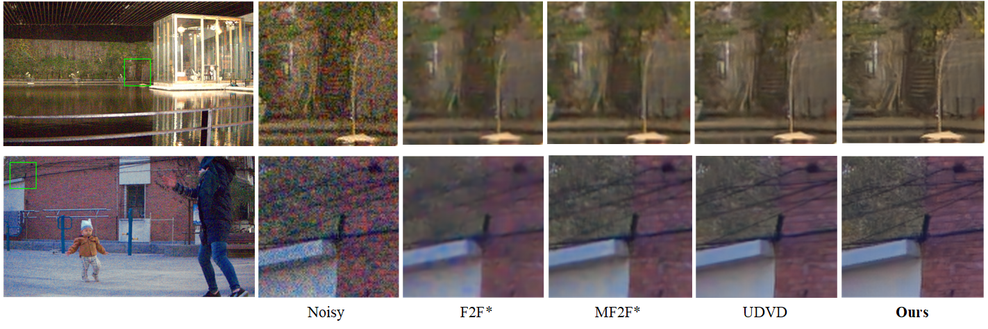
Figure 14: Visual quality comparison on CRVD outdoor test set for unsupervised raw video denoising methods which are trained with ReCRVD dataset. Zoom in for better observation.

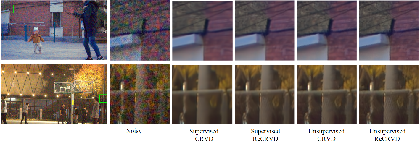
Figure 15: Visual quality comparison on CRVD outdoor test set for our model trained with different datasets. Zoom in for better observation.

To demonstrate the effectiveness of our proposed ReCRVD dataset and raw video denoising method RViDeformer, we use the CRVD outdoor test set [12] for further evaluation. CRVD outdoor test set contains 50 videos (containing 10 outdoor scenes with differnet ISO settings), which are captured naturally in real world but do not have ground truths. Therefore, we utilize no-reference image quality assessment metrics NRQM [68], NIQE [69], PI [70] and BRISQUE [71] to evaluate the video denoising results on this dataset. Table VII lists the quantitative comparison results for supervised raw video denoising. Table VIII lists the quantitative comparison results for unsupervised raw video denoising. Compared with training on CRVD indoor dataset, our model (RViDeformer-L) can achieve better results on all of the four metrics when training on our proposed ReCRVD dataset for both supervised and unsupervised learning. It verifies that our proposed ReCRVD dataset is a better benchmark dataset than CRVD due to the realistic motions and large amount of videos in ReCRVD. Compared with other video denoising methods, our method achieves the best results on all of the four metrics for both supervised and unsupervised learning, which demonstrates that our method has the best ability of generalization.

Note that, our model (RViDeformer-L) achieves better results via unsupervised training other than supervised training on CRVD outdoor test set. It implies that unsupervised training is beneficial for generating details for the dataset which has different distributions from the training set. Fig. 13 and 14 present the visual comparison results on the CRVD outdoor test set for both supervised and unsupervised raw video denoising methods, respectively. It can be observed that our method removes the noise clearly and recovers the most details, which also demonstrates that our method has the best ability of generalization for raw noisy videos which are captured naturally. Fig. 15 further presents the visual comparison results for our method trained with ReCRVD and CRVD datasets, respectively. It can be observed that training on ReCRVD dataset brings more natural details for both supervised and unsupervised learning, such as the tree and wall in the first scene, the tree and fence in the second scene. This further demonstrates that the noise model of our ReCRVD dataset is consistent with the noise model of real-world scenes.

TABLE VII: Quantitative comparisons of no-reference metrics for supervised raw video denoising on CRVD outdoor test set.

Methods	Training Set	NRQM$\uparrow$	NIQE$\downarrow$	PI$\downarrow$	BRISQUE$\downarrow$
Fastdvdnet	ReCRVD	6.7674	5.5646	3.5120	43.1539
EMVD	ReCRVD	6.7411	5.7329	3.6127	43.2835
BSVD-32	ReCRVD	6.9388	5.5462	3.4147	42.6387
RViDeformer-M	ReCRVD	6.9458	5.3654	3.3544	41.4491
RViDeNet	ReCRVD	6.7092	5.5260	3.5559	42.2494
FloRNN	ReCRVD	7.0097	5.3695	3.2999	41.7365
RVRT	ReCRVD	6.8863	5.3357	3.4057	41.5114
VRT	ReCRVD	6.9962	5.3049	3.3034	41.3907
RViDeformer-L	CRVD indoor	6.5539	5.1542	3.6137	42.3270
RViDeformer-L	ReCRVD	7.0158	5.1520	3.2380	41.0332

TABLE VIII: Quantitative comparisons of no-reference metrics for unsupervised raw video denoising on CRVD outdoor test set.

Methods	Training Set	NRQM$\uparrow$	NIQE$\downarrow$	PI$\downarrow$	BRISQUE$\downarrow$
F2F	ReCRVD	5.5262	6.8793	4.6866	52.8171
MF2F	ReCRVD	6.3266	6.0470	3.9249	44.9937
UDVD	ReCRVD	6.7882	5.4274	3.3932	42.0245
RViDeformer-L	CRVD indoor	6.8498	5.1097	3.2502	40.3322
RViDeformer-L	ReCRVD	7.2777	5.0696	3.0271	37.8852

6 Conclusion

In this work, we construct a benchmark dataset (ReCRVD) for raw video denoising to facilitate futher works on raw video denoising. Compared with CRVD, the motions in ReCRVD are real and the number of scenes (120) is much larger. Correspondingly we propose an efficient raw video denoising transformer network (RViDeformer), which is mainly constructed by multi-branch spatial self-attention and multi-branch temporal self-attention blocks. RViDeformer is evaluated by supervised learning and unsupervised learning, and it achieves the best results on both ReCRVD and CRVD datasets for both the two learning manners. In addition, the models trained on ReCRVD outperforms that trained on CRVD when testing on the third real test set (CRVD outdoor), which demonstrates that the noise model of ReCRVD is consistent with that of real-world noisy videos.

References

- [1] J. Lehtinen, J. Munkberg, J. Hasselgren, S. Laine, T. Karras, M. Aittala, and T. Aila, “Noise2noise: Learning image restoration without clean data,” arXiv preprint arXiv:1803.04189, 2018.
- [2] A. Krull, T.-O. Buchholz, and F. Jug, “Noise2void-learning denoising from single noisy images,” in Proceedings of the IEEE Conference on Computer Vision and Pattern Recognition, 2019, pp. 2129–2137.
- [3] Z. Wang, J. Liu, G. Li, and H. Han, “Blind2unblind: Self-supervised image denoising with visible blind spots,” in Proceedings of the IEEE/CVF Conference on Computer Vision and Pattern Recognition, 2022, pp. 2027–2036.
- [4] T. Ehret, A. Davy, J.-M. Morel, G. Facciolo, and P. Arias, “Model-blind video denoising via frame-to-frame training,” in Proceedings of the IEEE Conference on Computer Vision and Pattern Recognition, 2019, pp. 11 369–11 378.
- [5] V. Dewil, J. Anger, A. Davy, T. Ehret, G. Facciolo, and P. Arias, “Self-supervised training for blind multi-frame video denoising,” in Proceedings of the IEEE/CVF winter conference on applications of computer vision, 2021, pp. 2724–2734.
- [6] D. Y. Sheth, S. Mohan, J. L. Vincent, R. Manzorro, P. A. Crozier, M. M. Khapra, E. P. Simoncelli, and C. Fernandez-Granda, “Unsupervised deep video denoising,” in Proceedings of the IEEE/CVF International Conference on Computer Vision, 2021, pp. 1759–1768.
- [7] M. Tassano, J. Delon, and T. Veit, “Fastdvdnet: Towards real-time deep video denoising without flow estimation,” in Proceedings of the IEEE/CVF Conference on Computer Vision and Pattern Recognition, 2020, pp. 1354–1363.
- [8] J. Li, X. Wu, Z. Niu, and W. Zuo, “Unidirectional video denoising by mimicking backward recurrent modules with look-ahead forward ones,” in European Conference on Computer Vision. Springer, 2022, pp. 592–609.
- [9] M. Song, Y. Zhang, and T. O. Aydın, “Tempformer: Temporally consistent transformer for video denoising,” in European Conference on Computer Vision. Springer, 2022, pp. 481–496.
- [10] J. Liang, J. Cao, Y. Fan, K. Zhang, R. Ranjan, Y. Li, R. Timofte, and L. Van Gool, “Vrt: A video restoration transformer,” arXiv preprint arXiv:2201.12288, 2022.
- [11] J. Liang, Y. Fan, X. Xiang, R. Ranjan, E. Ilg, S. Green, J. Cao, K. Zhang, R. Timofte, and L. Van Gool, “Recurrent video restoration transformer with guided deformable attention,” arXiv preprint arXiv:2206.02146, 2022.
- [12] H. Yue, C. Cao, L. Liao, R. Chu, and J. Yang, “Supervised raw video denoising with a benchmark dataset on dynamic scenes,” in Proceedings of the IEEE/CVF Conference on Computer Vision and Pattern Recognition, 2020, pp. 2301–2310.
- [13] Z. Kong, X. Yang, and L. He, “A comprehensive comparison of multi-dimensional image denoising methods,” arXiv preprint arXiv:2011.03462, 2020.
- [14] Y. Fu, Z. Wang, T. Zhang, and J. Zhang, “Low-light raw video denoising with a high-quality realistic motion dataset,” IEEE Transactions on Multimedia, 2022.
- [15] Z. Liu, Y. Lin, Y. Cao, H. Hu, Y. Wei, Z. Zhang, S. Lin, and B. Guo, “Swin transformer: Hierarchical vision transformer using shifted windows,” in Proceedings of the IEEE/CVF International Conference on Computer Vision, 2021, pp. 10 012–10 022.
- [16] J. Liang, J. Cao, G. Sun, K. Zhang, L. Van Gool, and R. Timofte, “Swinir: Image restoration using swin transformer,” in Proceedings of the IEEE/CVF international conference on computer vision, 2021, pp. 1833–1844.
- [17] T. Huang, S. Li, X. Jia, H. Lu, and J. Liu, “Neighbor2neighbor: Self-supervised denoising from single noisy images,” in Proceedings of the IEEE/CVF conference on computer vision and pattern recognition, 2021, pp. 14 781–14 790.
- [18] K. Zhang, W. Zuo, Y. Chen, D. Meng, and L. Zhang, “Beyond a gaussian denoiser: Residual learning of deep cnn for image denoising,” IEEE Transactions on Image Processing, vol. 26, no. 7, pp. 3142–3155, 2017.
- [19] K. Zhang, W. Zuo, and L. Zhang, “Ffdnet: Toward a fast and flexible solution for cnn-based image denoising,” IEEE Transactions on Image Processing, vol. 27, no. 9, pp. 4608–4622, 2018.
- [20] W. Dong, P. Wang, W. Yin, G. Shi, F. Wu, and X. Lu, “Denoising prior driven deep neural network for image restoration,” IEEE transactions on pattern analysis and machine intelligence, vol. 41, no. 10, pp. 2305–2318, 2018.
- [21] S. Guo, Z. Yan, K. Zhang, W. Zuo, and L. Zhang, “Toward convolutional blind denoising of real photographs,” in Proceedings of the IEEE Conference on Computer Vision and Pattern Recognition, 2019, pp. 1712–1722.
- [22] C. Chen, Z. Xiong, X. Tian, Z.-J. Zha, and F. Wu, “Real-world image denoising with deep boosting,” IEEE transactions on pattern analysis and machine intelligence, vol. 42, no. 12, pp. 3071–3087, 2019.
- [23] Y. Zhang, Y. Tian, Y. Kong, B. Zhong, and Y. Fu, “Residual dense network for image restoration,” IEEE Transactions on Pattern Analysis and Machine Intelligence, 2020.
- [24] M. Matteo, G. Boracchi, F. Alessandro, E. Karen et al., “Video denoising using separable 4d nonlocal spatiotemporal transforms.” in Image Processing: Algorithms and Systems IX. SPIE, 2011, pp. 1–11.
- [25] X. Chen, L. Song, and X. Yang, “Deep rnns for video denoising,” in Applications of Digital Image Processing XXXIX, vol. 9971. International Society for Optics and Photonics, 2016, p. 99711T.
- [26] T. Xue, B. Chen, J. Wu, D. Wei, and W. T. Freeman, “Video enhancement with task-oriented flow,” International Journal of Computer Vision, vol. 127, no. 8, pp. 1106–1125, 2019.
- [27] M. Maggioni, Y. Huang, C. Li, S. Xiao, Z. Fu, and F. Song, “Efficient multi-stage video denoising with recurrent spatio-temporal fusion,” in Proceedings of the IEEE/CVF Conference on Computer Vision and Pattern Recognition, 2021, pp. 3466–3475.
- [28] C. Qi, J. Chen, X. Yang, and Q. Chen, “Real-time streaming video denoising with bidirectional buffers,” in Proceedings of the 30th ACM International Conference on Multimedia, 2022, pp. 2758–2766.
- [29] D. Li, X. Shi, Y. Zhang, X. Wang, H. Qin, and H. Li, “No attention is needed: Grouped spatial-temporal shift for simple and efficient video restorers,” arXiv preprint arXiv:2206.10810, 2022.
- [30] T. Pang, H. Zheng, Y. Quan, and H. Ji, “Recorrupted-to-recorrupted: unsupervised deep learning for image denoising,” in Proceedings of the IEEE/CVF conference on computer vision and pattern recognition, 2021, pp. 2043–2052.
- [31] X. Xu, Y. Ma, and W. Sun, “Towards real scene super-resolution with raw images,” in Proceedings of the IEEE Conference on Computer Vision and Pattern Recognition, 2019, pp. 1723–1731.
- [32] X. Zhang, Q. Chen, R. Ng, and V. Koltun, “Zoom to learn, learn to zoom,” in Proceedings of the IEEE Conference on Computer Vision and Pattern Recognition, 2019, pp. 3762–3770.
- [33] H. Yue, Z. Zhang, and J. Yang, “Real-rawvsr: Real-world raw video super-resolution with a benchmark dataset,” in European Conference on Computer Vision. Springer, 2022, pp. 608–624.
- [34] S. Ratnasingam, “Deep camera: A fully convolutional neural network for image signal processing,” in Proceedings of the IEEE International Conference on Computer Vision Workshops, 2019, pp. 0–0.
- [35] E. Schwartz, R. Giryes, and A. M. Bronstein, “Deepisp: learning end-to-end image processing pipeline,” arXiv preprint arXiv:1801.06724, 2018.
- [36] Z. Liang, J. Cai, Z. Cao, and L. Zhang, “Cameranet: A two-stage framework for effective camera isp learning,” arXiv preprint arXiv:1908.01481, 2019.
- [37] A. Ignatov, R. Timofte, Z. Zhang, M. Liu, H. Wang, W. Zuo, J. Zhang, R. Zhang, Z. Peng, S. Ren et al., “Aim 2020 challenge on learned image signal processing pipeline,” arXiv preprint arXiv:2011.04994, 2020.
- [38] C.-H. Liang, Y.-A. Chen, Y.-C. Liu, and W. Hsu, “Raw image deblurring,” IEEE Transactions on Multimedia, 2020.
- [39] H. Yue, Y. Cheng, Y. Mao, C. Cao, and J. Yang, “Recaptured screen image demoiréing in raw domain,” IEEE Transactions on Multimedia, 2022.
- [40] M. Gharbi, G. Chaurasia, S. Paris, and F. Durand, “Deep joint demosaicking and denoising,” ACM Transactions on Graphics (TOG), vol. 35, no. 6, p. 191, 2016.
- [41] C. Chen, Q. Chen, M. N. Do, and V. Koltun, “Learning to see in the dark,” in Proceedings of the IEEE Conference on Computer Vision and Pattern Recognition, 2018.
- [42] J. Liu, C.-H. Wu, Y. Wang, Q. Xu, Y. Zhou, H. Huang, C. Wang, S. Cai, Y. Ding, H. Fan et al., “Learning raw image denoising with bayer pattern unification and bayer preserving augmentation,” in Proceedings of the IEEE Conference on Computer Vision and Pattern Recognition Workshops, 2019, pp. 0–0.
- [43] A. Abdelhamed, R. Timofte, and M. S. Brown, “Ntire 2019 challenge on real image denoising: Methods and results,” in Proceedings of the IEEE Conference on Computer Vision and Pattern Recognition Workshops, 2019, pp. 0–0.
- [44] A. Abdelhamed, M. Afifi, R. Timofte, and M. S. Brown, “Ntire 2020 challenge on real image denoising: Dataset, methods and results,” in Proceedings of the IEEE/CVF Conference on Computer Vision and Pattern Recognition Workshops, 2020, pp. 496–497.
- [45] J. Anaya and A. Barbu, “Renoir-a dataset for real low-light image noise reduction,” arXiv preprint arXiv:1409.8230, 2014.
- [46] A. Abdelhamed, S. Lin, and M. S. Brown, “A high-quality denoising dataset for smartphone cameras,” in Proceedings of the IEEE Conference on Computer Vision and Pattern Recognition, 2018, pp. 1692–1700.
- [47] T. Plotz and S. Roth, “Benchmarking denoising algorithms with real photographs,” in Proceedings of the IEEE Conference on Computer Vision and Pattern Recognition, 2017, pp. 1586–1595.
- [48] T. Brooks, B. Mildenhall, T. Xue, J. Chen, D. Sharlet, and J. T. Barron, “Unprocessing images for learned raw denoising,” CVPR, 2019.
- [49] S. W. Zamir, A. Arora, S. Khan, M. Hayat, F. S. Khan, M.-H. Yang, and L. Shao, “Cycleisp: Real image restoration via improved data synthesis,” in Proceedings of the IEEE/CVF Conference on Computer Vision and Pattern Recognition, 2020, pp. 2696–2705.
- [50] Y. Wang, H. Huang, Q. Xu, J. Liu, Y. Liu, and J. Wang, “Practical deep raw image denoising on mobile devices,” in European Conference on Computer Vision. Springer, 2020, pp. 1–16.
- [51] C. Chen, Q. Chen, M. N. Do, and V. Koltun, “Seeing motion in the dark,” in Proceedings of the IEEE International Conference on Computer Vision, 2019.
- [52] S. Nam, Y. Hwang, Y. Matsushita, and S. Joo Kim, “A holistic approach to cross-channel image noise modeling and its application to image denoising,” in Proceedings of the IEEE Conference on Computer Vision and Pattern Recognition, 2016, pp. 1683–1691.
- [53] H. Yue, J. Liu, J. Yang, T. Nguyen, and F. Wu, “High iso jpeg image denoising by deep fusion of collaborative and convolutional filtering,” IEEE Transactions on Image Processing, 2019.
- [54] J. Xu, H. Li, Z. Liang, D. Zhang, and L. Zhang, “Real-world noisy image denoising: A new benchmark,” arXiv preprint arXiv:1804.02603, 2018.
- [55] X. Xu, Y. Yu, N. Jiang, J. Lu, B. Yu, and J. Jia, “Pvdd: A practical video denoising dataset with real-world dynamic scenes,” arXiv preprint arXiv:2207.01356, 2022.
- [56] Y. Peng, Q. Sun, X. Dun, G. Wetzstein, W. Heidrich, and F. Heide, “Learned large field-of-view imaging with thin-plate optics.” ACM Trans. Graph., vol. 38, no. 6, pp. 219–1, 2019.
- [57] F. Perazzi, J. Pont-Tuset, B. McWilliams, L. Van Gool, M. Gross, and A. Sorkine-Hornung, “A benchmark dataset and evaluation methodology for video object segmentation,” in Proceedings of the IEEE conference on computer vision and pattern recognition, 2016, pp. 724–732.
- [58] A. Mercat, M. Viitanen, and J. Vanne, “Uvg dataset: 50/120fps 4k sequences for video codec analysis and development,” in Proceedings of the 11th ACM Multimedia Systems Conference, 2020, pp. 297–302.
- [59] S. Su, M. Delbracio, J. Wang, G. Sapiro, W. Heidrich, and O. Wang, “Deep video deblurring for hand-held cameras,” in Proceedings of the IEEE conference on computer vision and pattern recognition, 2017, pp. 1279–1288.
- [60] T. Thongkamwitoon, H. Muammar, and P.-L. Dragotti, “An image recapture detection algorithm based on learning dictionaries of edge profiles,” IEEE Transactions on Information Forensics and Security, vol. 10, no. 5, pp. 953–968, 2015.
- [61] P. Weinzaepfel, J. Revaud, Z. Harchaoui, and C. Schmid, “Deepflow: Large displacement optical flow with deep matching,” in Proceedings of the IEEE international conference on computer vision, 2013, pp. 1385–1392.
- [62] C.-F. R. Chen, Q. Fan, and R. Panda, “Crossvit: Cross-attention multi-scale vision transformer for image classification,” in Proceedings of the IEEE/CVF international conference on computer vision, 2021, pp. 357–366.
- [63] Y. Chen, X. Dai, D. Chen, M. Liu, X. Dong, L. Yuan, and Z. Liu, “Mobile-former: Bridging mobilenet and transformer,” in Proceedings of the IEEE/CVF Conference on Computer Vision and Pattern Recognition, 2022, pp. 5270–5279.
- [64] X. Zhang, H. Zeng, S. Guo, and L. Zhang, “Efficient long-range attention network for image super-resolution,” in Computer Vision–ECCV 2022: 17th European Conference, Tel Aviv, Israel, October 23–27, 2022, Proceedings, Part XVII. Springer, 2022, pp. 649–667.
- [65] X. Ding, X. Zhang, J. Han, and G. Ding, “Diverse branch block: Building a convolution as an inception-like unit,” in Proceedings of the IEEE/CVF Conference on Computer Vision and Pattern Recognition, 2021, pp. 10 886–10 895.
- [66] P. K. Ostrowski, E. Katsaros, D. Wesierski, and A. Jezierska, “Bp-evd: Forward block-output propagation for efficient video denoising,” IEEE Transactions on Image Processing, vol. 31, pp. 3809–3824, 2022.
- [67] X. Wang, K. C. Chan, K. Yu, C. Dong, and C. Change Loy, “Edvr: Video restoration with enhanced deformable convolutional networks,” in Proceedings of the IEEE Conference on Computer Vision and Pattern Recognition Workshops, 2019, pp. 0–0.
- [68] C. Ma, C.-Y. Yang, X. Yang, and M.-H. Yang, “Learning a no-reference quality metric for single-image super-resolution,” Computer Vision and Image Understanding, vol. 158, pp. 1–16, 2017.
- [69] A. Mittal, R. Soundararajan, and A. C. Bovik, “Making a “completely blind” image quality analyzer,” IEEE Signal processing letters, vol. 20, no. 3, pp. 209–212, 2012.
- [70] Y. Blau, R. Mechrez, R. Timofte, T. Michaeli, and L. Zelnik-Manor, “The 2018 pirm challenge on perceptual image super-resolution,” in Proceedings of the European Conference on Computer Vision (ECCV) Workshops, 2018, pp. 0–0.
- [71] A. Mittal, A. K. Moorthy, and A. C. Bovik, “Blind/referenceless image spatial quality evaluator,” in 2011 conference record of the forty fifth asilomar conference on signals, systems and computers (ASILOMAR). IEEE, 2011, pp. 723–727.