Full Scaling Automation for Sustainable Development of Green Data Centers

Abstract

The rapid rise in cloud computing has resulted in an alarming increase in data centers’ carbon emissions, which now account for $>$3% of global greenhouse gas emissions, necessitating immediate steps to combat their mounting strain on the global climate. An important focus of this effort is to improve resource utilization in order to save electricity usage. Our proposed Full Scaling Automation (FSA) mechanism is an effective method of dynamically adapting resources to accommodate changing workloads in large-scale cloud computing clusters, enabling the clusters in data centers to maintain their desired CPU utilization target and thus improve energy efficiency. FSA harnesses the power of deep representation learning to accurately predict the future workload of each service and automatically stabilize the corresponding target CPU usage level, unlike the previous autoscaling methods, such as Autopilot or FIRM, that need to adjust computing resources with statistical models and expert knowledge. Our approach achieves significant performance improvement compared to the existing work in real-world datasets. We also deployed FSA on large-scale cloud computing clusters in industrial data centers, and according to the certification of the China Environmental United Certification Center (CEC), a reduction of 947 tons of carbon dioxide, equivalent to a saving of 1538,000 kWh of electricity, was achieved during the Double 11 shopping festival of 2022, marking a critical step for our company’s strategic goal towards carbon neutrality by 2030.

1 Introduction

As the demand for data and cloud computing services continues to soar, the data center industry is expanding at a staggering rate, serving as the backbone of the economic, commercial, and social lives of the modern world. The data centers are, however, some of the world’s biggest consumers of electrical energy, and their ever-increasing carbon emissions only exacerbate global warming. Currently, the emissions from data centers compose 3.7% of all global greenhouse gas emissionsclimatiq.io (2021), exceeding those from commercial flights and other existential activities that fuel our economy. This attracts the concern of many global organizations, including United Nations’ climate conferences focusing on sustainability in data centersUN (2021); Campbell (2017). As part of the worldwide effort towards carbon neutrality (or net zero carbon), making more efficient use of data centers’ computing resources becomes an increasingly popular research area to minimize the energy consumption.

The carbon emissions of large-scale cloud computing clusters in data centers mainly come from the power consumption of equipment loads. Several studies have shown that servers running with chronically low CPU utilization are one major source of energy wasting, which can be alleviated by reducing the amount of resources allocated for low-load services, and reallocating those saved servers to high-load servicesKrieger et al. (2017); Abdullah et al. (2020). Efficient resource allocation mechanism thus serves an important role in this effort. Moreover, some systems allow flexibly shutting down unneeded servers to further save the power consumption with proper scheduling and engineering mechanism. To this extent, most cloud computing providers try to take advantage of automatic scaling systems (autoscaling) to stabilize the CPU utilization of the systems being provisioned to the desired target levels, not only to ensure their services meet the stringent Service Level Objectives (SLOs), but also to prevent CPUs from running at low utilizationQiu et al. (2020).

Specifically, autoscaling elastically scales the resources horizontally (i.e., changing the number of virtual Containers (Pods) assigned) or vertically (i.e., adjusting the CPU and memory reservations) to match the varying workload according to certain performance measure, such as resource utility. Prior work on cloud autoscaling can be categorized as rule-based or learning-based schemes. Rule-based mechanism sets thresholds of metrics (such as CPU utilization and workload ) based on expert experience and monitors indicator changes to facilitate resource scheduling. Learning-based autoscaling mechanism employs statistical or machine learning to model historical patterns to generate scaling strategies. However, the existing works face the following challenges:

• Challenge 1: Forecasting time series (TS) of workloads with complex periodic and long temporal dependencies. Most autoscaling studies focus on decision-making processes of scaling rather than server workload forecasting, eluding the critical task of accurately predicting future workloads (normally non-stationary TS of high-frequency with various periods and complex long temporal dependencies), which are not well-handled by existing work employing classic statistical methods (such as ARIMA) or simple neural networks (such as RNN).

• Challenge 2: Maintaining stable CPU utilization and characterizing uncertainty in the decision-making process. Most methods aim at adequately utilizing resources for cost-savings while ignoring the stability measures of the service, such as the robustness and SLOs assurances, where stable CPU utilization is of great significance. Moreover, affected by various aspects of the servers (such as temperature), the uncertainty of the correlation between CPU utilization and workload needs to be modeled in the decision-making process to balance between benefits and risks.

• Challenge 3: Accounting for sustainable development of green data centers. Existing works only optimize resources and costs, instead of carbon emissions, which is one essential task for the sustainable green data centers.

To this extent, we propose in this paper a novel predictive horizontal autoscaling named Full Scaling Automation (FSA) to tackle the above difficulties. Specifically, first, we develop an original workload forecasting framework based on representation learning, i.e., we learn multi-scale representations from historical workload TS as external memory, characterizing long temporal dependencies and complex various periodic (such as days, weeks and months). We then build a representation-enhanced deep autoregressive model, which integrates multi-scale representations and near-observation TS via multi-head self-attention. Second, we propose a task-conditioned Bayesian neural model to learn the relationship between CPU utilization and workload, enabling the characterization of the uncertainty between them, while providing the upper and lower bounds of benefits and risks. Moreover, with the help of the task-conditioned hypernetwork Mahabadi et al. (2021); He et al. (2022), our approach can be easily adapted to various online scenarios. Third, based on the workload forecasting and CPU utilization estimation above, we can properly pre-allocate resources and distribute the future workload to each machine, targeting certain CPU utilization level, maximizing energy efficiency.

We have deployed our FSA mechanism on large-scale cloud computing clusters, and with the help of China Environmental United Certification Center (CEC), one can convert between energy saving and carbon emission reduction, aiming at sustainable development in data centers. To the best of our knowledge, we are the first in the industry to employ AI-based resource scaling for this goal.

Our Contributions can be summarized as follows:

• A novel workload probabilistic forecast framework with the representation-enhanced deep autoregressive model, integrating multi-scale TS representation.

• A task-conditioned Bayesian neural model estimating the uncertainty between CPU utilization and workload.

• An efficient predictive horizontal autoscaling mechanism to stabilize CPU utilization, saving costs and energy, facilitating sustainable data centers.

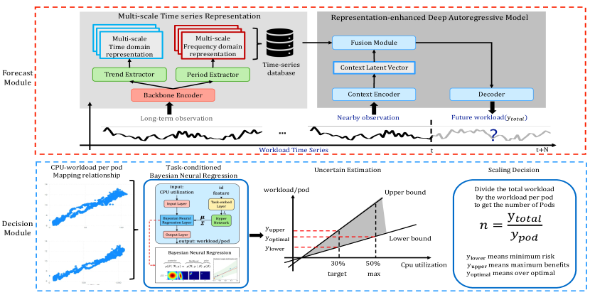
Figure 1: Model Architecture. Red dashed lines represent the workload forecast module, including Multi-scale Time Series Representation and Representation-enhanced Deep Autoregressive Model. Blue dashed lines highlight the scaling decision module via task-conditioned Bayesian neural regression. According to service tolerance for response time(rt), the optimal value between upper and lower bounds is obtained.

2 Background And Related Work

2.1 Horizontal Autoscaling

Horizontal autoscaling is a practical resource management method that elastically scales the resources horizontally (i.e., changing the number of virtual Containers (Pods) assigned) Nguyen et al. (2020). Most existing studies focus on avoiding service anomalies, e.g., FIRM Qiu et al. (2020) uses machine learning to detect service performance anomalies (e.g., the RT of a microservice is abnormally long) and when such anomalies occur, more Pods are allocated; Autopilot Rzadca et al. (2020) takes TS of the CPU utilization of a microservice as input, and employs a simple heuristic mechanism to obtain the target CPU utilization, which is then used to calculate the number of Pods required as a linear function. Pods are increased or reduced to minimize the risk that a microservice suffers from anomalies. These methods have the following limitations: (1) Most methods are reactive scaling, i.e., autoscaling occurs only after performance anomalies occur. (2) Due to the lack of workload forecasting mechanism, making precise decision for future resource scaling is difficult. (3) The uncertainty of CPU utilization is not considered in decision making, leading to unknown risks in resource scaling.

2.2 Workload Forecasting

One key constituent of our method is forecasting the workload, which is, however, normally of high-frequency and non-stationary with various periods and complex long temporal dependencies, defying most classic TS forecasting models. We therefore propose to use TS representations to memorize long-term temporal dependencies to battle this complexity.

Time Series (TS) Forecasting. Deep forecasting methods based on RNN or Transformer, including N-beats, Informer, and DeepAR, etc., have been widely applied to TS forecasting, outperforming classical models such as ARIMA and VAR. N-BEATS is an interpretable TS forecasting model, with deep neural architecture based on backward and forward residual links with a very deep stack of fully-connected layersOreshkin et al. (2019). Informer is a prob-sparse self-attention mechanism-based model to enhance the prediction capacity in the long-sequence TS forecasting problems, which validates the Transformer-like model’s potential value to capture individual long-range dependency between long sequence TS outputs and inputs Zhou et al. (2021). DeepAR is a probabilistic autoregressive forecasting model based on RNN, widely applied in real-world industrial applications Salinas et al. (2020).

Time Series (TS) Representation. Representation learning has recently achieved great success in advancing TS research by characterizing the long temporal dependencies and complex periodicity based on the contrastive method. TS-TCC creates two views for each sample by applying strong and weak augmentations and then using the temporal contrasting module to learn robust temporal features by applying a cross-view prediction task Eldele et al. (2021). TS2Vec was recently proposed as a universal framework for learning TS representations by performing contrastive learning in a hierarchical loss over augmented context views Yue et al. (2022). A new TS representation learning framework was proposed in CoST for long-sequence TS forecasting, which applies contrastive learning methods to learn disentangled seasonal-trend representations Woo et al. (2022).

2.3 Bayesian Method

Bayesian methods are frequently used to model uncertainties of the variables, and are introduced to deep learning models to improve robustness of the model Bishop and Nasrabadi (2006). In this work, we introduce task-conditioned hypernetwork Mahabadi et al. (2021) into Bayesian regression to estimate the correlation between CPU utilization and workload.

3 Proposed Methodology

In this section, we detail our framework, including the forecast module and decision module, as shown in Figure 1.

3.1 Problem Definition

Let us denote the value of TS of workload by $y_{t}\in\mathbb{R}^{F}$, where $t$ indexes time on a time horizon $t\in\{1,2,...,T\}$, and $F$ is the dimension of features, such as time feature and id feature.

Given the historical workload TS of an application $y_{t-L}$ at time $t$, we aim to find the optimal Pods allocated over the future time horizon $N$ to make the application run stably around a target CPU utilization. We assume the total workload of an application is evenly allocated across all Pods via load balancing and we can represent their relationship as

$$y^{pod}_{t}={y^{total}_{t}}/{n_{t}}\quad\Leftrightarrow\quad n_{t}={y^{total}_{t}}/{y^{pod}_{t}}\mbox{ ,}$$ (1)

where $y^{total}_{t}$ is the total workload, $y^{pod}_{t}$ is the workload per Pod, and $n_{t}$ is the number of Pods at time $t$. Please note that this assumption is ensured by our software and hardware engineering platform of the data centers.

3.2 Workload Forecasting

Considering that the workload TS are non-stationary and of high-frequency (one minute scale) with various periods and complex long temporal dependencies (such as daily, weekly, monthly, and even quarterly periodicities) and existing work requires backcasts on long historical time windows as the input of the context. The formidable amount of data makes memorizing the historical data and learning these temporal dependencies difficult. Therefore, we propose a TS time series representation method, which characterizes complex long-term historical TS with various periodicity as compressed representation vectors and stores them in the TS database. We then design a CNF-based deep autoregressive fusing model, which integrates long-term historical TS representations and short-term observations (nearby window) to achieve accurate predictions.

3.2.1 Multi-scale Time Series (TS) Representation

Given TS $y\in\mathbb{R}^{T\times F}$ with backcast window $h$, our goal is to learn a nonlinear embedding function $f_{\theta}$ that maps $\{y_{t-h}...y_{t}\}$ to its representation $r_{t}=[r^{T}_{t},r^{F}_{t}]$, where $r_{t}\in\mathbb{R}^{K}$ is for each time stamp $t$, $r^{T}_{t}\in\mathbb{R}^{K_{T}}$ is the time domain representation, $r^{F}_{t}\in\mathbb{R}^{K_{F}}$ denotes that of frequency domain and $K=K_{T}+K_{F}$ is the dimension of representation vectors. In the encoding representation stage, by using backcast windows of various lengths, we can obtain a representation of different scales.

A schematic view of representation generation is shown in Figure 2. We first randomly sample two overlapping subseries from an input TS and then perform data augmentation separately. Next, using Multilayer Perceptron (MLP) as the input projection layer, the original input ${y_{t}}$ is mapped into a high-dimensional latent vector ${z_{t}}$. We use timestamp masking to mask latent vectors at randomly selected timestamps to generate an augmented context view. We then use CovnTrans as the backbone encoder to extract the contextual embedding at each timestamp. Subsequently, we extract the trends in the time domain and the period in the frequency domain using CausalConv and Fast Fourier transform (FFT) from the contextual embedding, respectively. Finally, we perform contrastive learning in the time and frequency domains. In the following sections, we describe these components in detail.

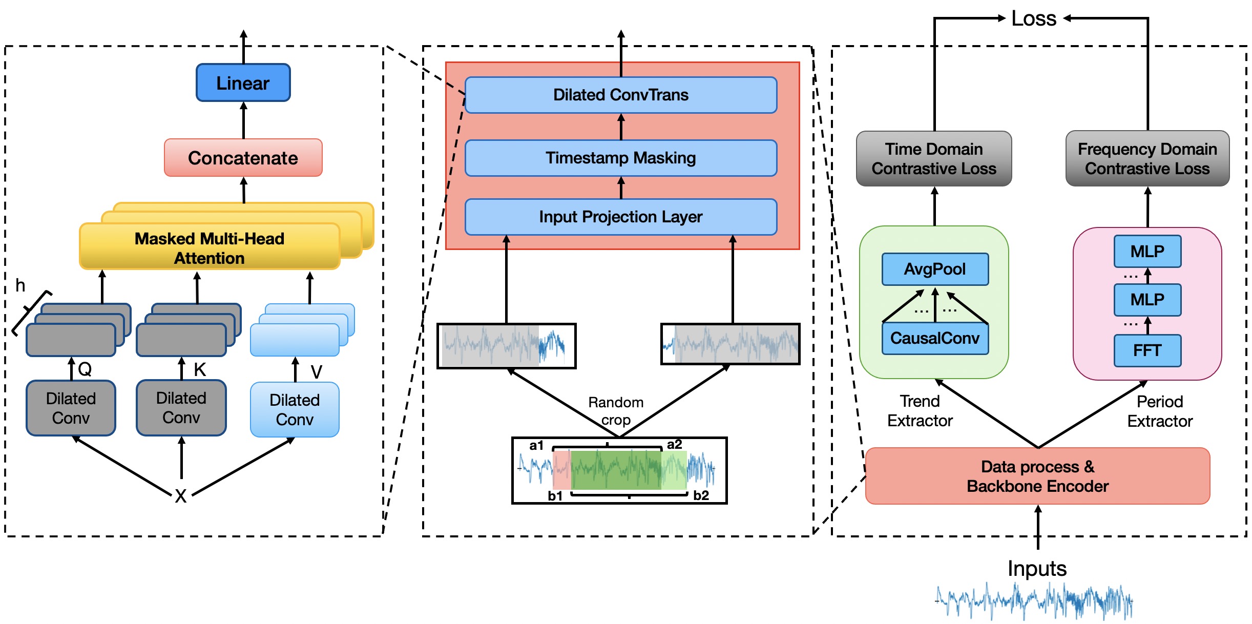
Figure 2: Multi-scale Time Series Representation

Random Cropping is a data augmentation method commonly used in contrastive learning to generate new context views. We can randomly sample two overlapping time segments $[a_{1},a_{2}]$ and $[b_{1},b_{2}]$ from TS $y\in\mathbb{R}^{T\times F}$ that satisfy $0<a_{1}<b_{1}<a_{2}<b_{2}$ $\leq$ $T$. Note that contextual representations on the overlapped segment $[b1,a2]$ ensure consistency for two context views.

Timestamp Masking aims to produce an augmented context view by randomly masking the timestamps of a TS. We can mask off the latent vector $z=\{z_{t}\}$ after the Input Projection Layer along the time axis with a binary mask $m\in\{0,1\}^{T}$, the elements of which are independently sampled from a Bernoulli distribution with $p=0.5$.

Backbone Encoder is used to extract the contextual representation at each timestamp. We use 1-layer causal convolution Transformer (ConvTrans) as our backbone encoder, which is enabled by its convolutional multi-head self-attention to capture both long- and short-term dependencies.

Specifically, given TS $y\in\mathbb{R}^{T\times F}$, ConvTrans transforms $y$ (as input) into dimension $l$ via dilated causal convolution layer as follows:

$$\begin{aligned} Q&=DilatedConv(y)\\ K&=DilatedConv(y)\\ V&=DilatedConv(y)\end{aligned}\mbox{ ,}$$

where $\bm{Q}\in\mathbb{R}^{dl\times dh}$, $\bm{K}\in\mathbb{R}^{dl\times dh}$, and $\bm{V}\in\mathbb{R}^{dl\times dh}$ (we denote the length of time steps as $dh$). After these transformations, the scaled dot-product attention computes the sequence of vector outputs via:

$${S}=\text{Attention}({Q},\ {K},\ {V})=\operatorname{softmax}\left({{Q}{K}^{T}}/{\sqrt{d_{K}}}\cdot{M}\right){V}\mbox{ ,}$$

where the mask matrix $M$ can be applied to filter out right-ward attention (or future information leakage) by setting its upper-triangular elements to $-\infty$ and normalization factor $d_{K}$ is the dimension of $W_{h}^{K}$ matrix. Finally, all outputs $S$ are concatenated and linearly projected again into the next layer. After the above series of operations, we use this backbone $f_{\theta}$ to extract the contextual embedding (intermediate representations ) at each timestamp as $\tilde{r}=f_{\theta}(y)$.

Time Domain Contrastive Learning. To extract the underlying trend of TS, one straightforward method is to use a set of 1d causal convolution layers (CasualConv) with different kernel sizes and an average-pooling operation to extract the representations as

$$\tilde{r}^{(T,i)}=CausalConv(\tilde{r},2^{i})$$

$$r^{T}=AvgPool(\tilde{r}^{(T,1)},\tilde{r}^{(T,2)}...,\tilde{r}^{(T,L)})\mbox{ ,}$$

where $L$ is a hyper-parameter denoting the number of CasualConv, $2^{i}$ ($i=0,...,L$) is the kernel size of each CasualConv, $\tilde{r}$ is above intermediate representations from the backbone encoder, followed by average-pool over the $L$ representations to obtain time domain representation $\tilde{r}^{(T)}$. To learn discriminative representations over time, we use the time domain contrastive loss, which takes the representations at the same timestamp from two views of the input TS as positive samples ($r^{T}_{i,t},\hat{r}^{T}_{i,t}$), while those at different timestamps from the same time series as negative samples, formulated as

$$\mathcal{L}_{time}=-log\frac{exp(r^{T}_{i,t}\cdot\hat{r}^{T}_{i,t})}{\sum_{t^{\prime}\in\mathcal{T}}(exp(r^{T}_{i,t}\cdot\hat{r}^{T}_{i,t^{\prime}})+\mathbb{I}(t\neq t^{\prime})exp(r^{T}_{i,t}\cdot r^{T}_{i,t^{\prime}})}$$

, where $\mathcal{T}$ is the set of timestamps within the overlap of the two subseries, subscript $i$ is the index of the input TS sample, and $t$ is the timestamp.

Frequency Domain Contrastive Learning. Considering that spectral analysis in frequency domain has been widely used in period detection, we use Fast Fourier Transforms (FFT) to map the above intermediate representations to the frequency domain to capture different periodic patterns. We can thus build a period extractor, including FFT and MLP, which extracts the frequency spectrum from the above contextual embedding and maps it to the freq-based representation $r^{F}_{t}$. To learn representations that are able to discriminate between different periodic patterns, we adopt the frequency domain contrastive loss indexed with $(i,t)$ along the instances of the batch, formulated as

$$\mathcal{L}_{Freq}=-log\frac{exp(r^{F}_{i,t}\cdot\hat{r}^{F}_{i,t})}{\sum_{j\in\mathcal{D}}(exp(r^{F}_{i,t}\cdot\hat{r}^{F}_{i,t^{\prime}})+\mathbb{I}(i\neq j)exp(r^{F}_{i,t}\cdot r^{F}_{i,t^{\prime}})}$$

, where $\mathcal{D}$ is defined as a batch of TS. We use freq-based representations of other TS at timestamp $t$ in the same batch as negative samples.

The contrastive loss is composed of two losses that are complementary to each other and is defined as

$$\begin{aligned} \mathcal{L}=\frac{1}{|\mathcal{D}|T}(\mathcal{L}_{time}+\mathcal{L}_{Freq})\end{aligned}\mbox{ ,}$$ (2)

where $\mathcal{D}$ denotes a batch of TS. As mentioned before, we pre-train our TS representation model, and in the encoding representation stage, by using backcast windows of various lengths, we can obtain a representation of different scales. In this paper, we encode the origin high-frequency TS(one-minute scale) to generate daily, weekly, monthly, and quarterly representations of long-term historical TS.

3.2.2 Representation-enhanced Deep Autoregressive Model

We now introduce the Representation-enhanced Deep Autoregressive Model in detail. Let us denote the values of TS by $y_{t}\in\mathbb{R}$, where $t$ indexes time on a time horizon $t\in\{1,2,...,T\}$. Note that we define $x_{t}$ as future knowable covariates, such as time feature and id feature, at time step $t$.

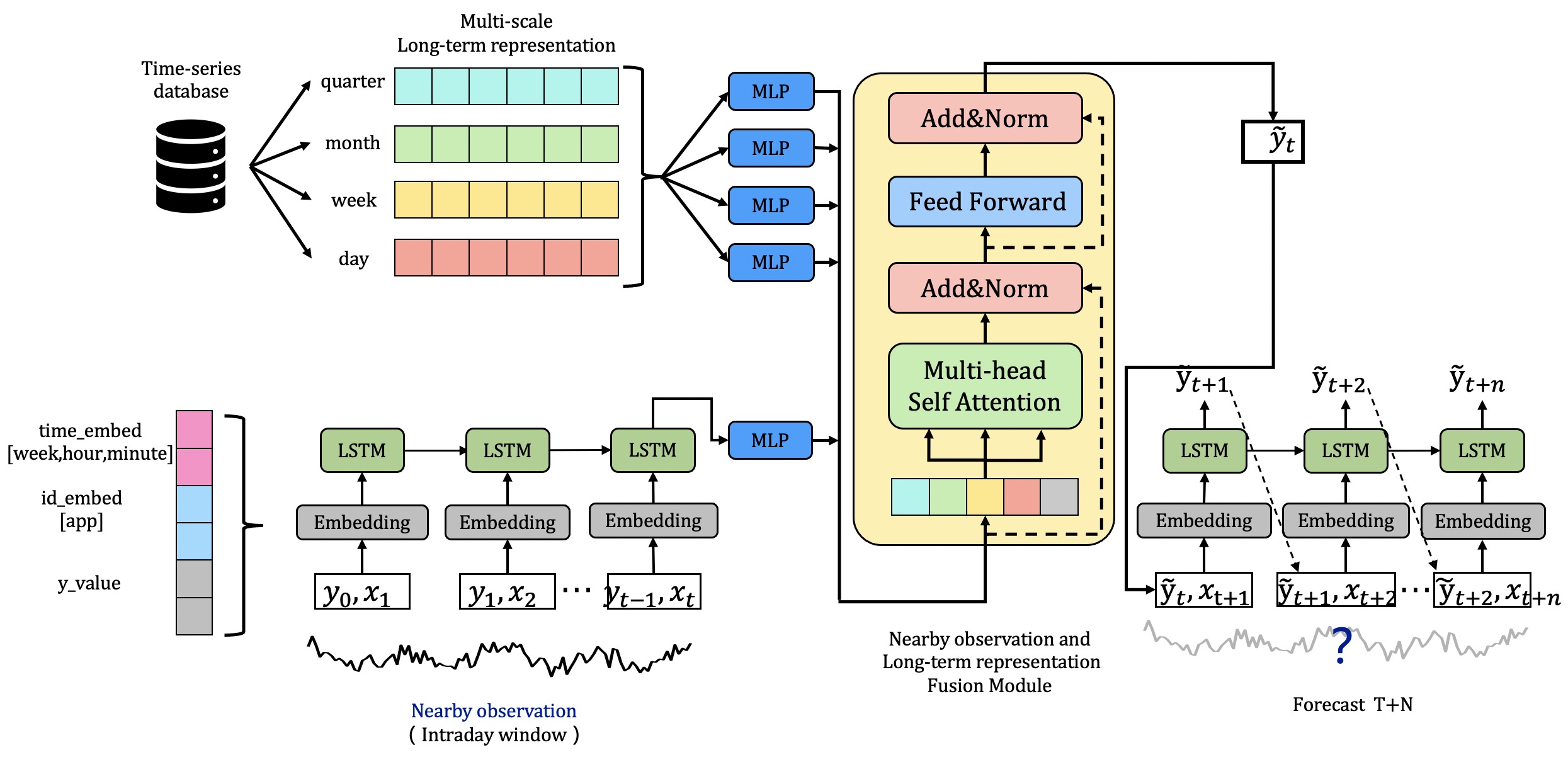
Figure 3: Representation-enhanced Deep Autoregressive Model

Given the last $L$ observations $y_{t-L},...,y_{t}$, the TS forecasting task aims to predict the future N observations $y_{t+1},...,y_{t+N}$. We use $r_{t}$, the representation of the long-term historical TS, and $h_{t}$ as the context latent vector from short-term observations (nearby window), to predict future observations.

Specifically, we first load the Multi-scale TS representation $r_{t}$ (including daily, weekly, monthly, and even quarterly) from the TS database, which characterizes various periods and complex long temporal dependencies. Secondly, we use the Recurrent Neural Network (RNN) to encode the short-term observations (nearby window) as a context latent vector $h_{t}$, which captures the intraday changing pattern of workload TS. We then use MLP to integrate them into the same dimension. Thirdly, inspired by the transformer architecture, we naturally use the multi-head self-attention as the fusion module that integrates long-term historical TS representations and short-term observations (nearby window) to achieve better predictions. This architecture enables us to capture not only the long-term dependency and periods of TS, but also the short-term changes within the day. Finally, with the help of RNN as the decoder, we perform autoregressive decoding to achieve multi-step prediction.

In the training, given $\mathcal{D}$, defined as a batch of TS $Y:=\{y_{1},y_{2},...,y_{T}\}$, the representation of the long-term historical TS as $r_{t}$, and the associated covariates $X:=\{x_{1},x_{2},...,x_{T}\}$, we can derive the likelihood as:

$$\begin{aligned} \mathcal{L}=\frac{1}{|\mathcal{D}|T}\prod_{x1:T,y1:T\in\mathcal{D}}\prod_{t=1}^{T}p(y_{t}|y_{1:t-1};x_{1:t},r_{t},\Phi)\end{aligned}\mbox{ ,}$$ (3)

where $\Phi$ is the learnable parameter of the model.

3.3 Scaling Decision

As mentioned before, we aim to find the optimal Pods allocated over the future time horizon $N$ to make the application run stably around a target CPU utilization, with the assumption that the total workload of an application is evenly allocated on all Pods by load balancing, i.e., the total future workload $y_{t}^{total}$ is evenly distributed over all Pods. Therefore, in order to obtain the number of scaling Pods, according to equation 1 above, our current key is to learn the relationship between CPU utilization and workload, for which, we propose Task-conditioned Bayesian Neural Regression.

3.3.1 Task-conditioned Bayesian Neural Regression

We propose a novel method that incorporates the task-conditioned hypernetwork and the Bayesian method to create a unified model that can adapt to varied scenarios online. This model is intended to address the uncertainty between CPU utilization and workload as described in Challenge 2. Specifically, our model takes the target CPU utilization $x_{cpu}$ and id feature $x_{id}$ of the app as input $X$, and output the per-Pod workload $y$. Our regression model ($y=w\cdot x_{cpu}+b$), adopts Bayesian neural networks Blundell et al. (2015) to provide the estimate of the uncertainty. The parameters $\beta$ include weight $w$ and bias $b$. We assume parameters $\beta$ follows probabilistic distribution, where the prior distribution is $p_{prior}(\beta)\sim\mathcal{N}(0,I)$, and the posterior distribution is $p_{posterior}(\beta|X,y)$. With the help of the variational Bayes, we can use the learnable model $q_{\phi}(\beta|X,y)\sim\mathcal{N}(\bm{\mu},\bm{\Sigma})$ as an approximation to the intractable true posterior distribution, where $\phi$ is the parameter of the model given by task conditioned information.

We first compute a task embedding $I_{\tau}$ for each scenario of the app, using a task projector network $h_{I}(\cdot)$, which is an MLP consisting of two feed-forward layers and a ReLU non-linearity:

$$\bm{I_{\tau}}=h_{I}(x_{id})\mbox{ ,}$$ (4)

where $x_{id}$ is the task feature above that indicates different scenarios of the app and the task projector network $h_{I}(\cdot)$ learns a suitable compressed task embedding from input task features.

We then define a simple linear layer of hypernetwork $g_{A}^{l}(\cdot)$, taking the task embeddings $I_{\tau}$ as input, to generate the parameter $\bm{\mu}$(mean) and $\bm{\Sigma}$(variance) of the above approximation distribution of $q_{\phi}(\beta|X,y)$ task-conditioned Bayesian model. In this way, we can provide different model parameters for each estimate of the app.

In the training stage, given $\mathcal{D}$, defined as a batch of data, with the Stochastic Gradient Variational Bayes (SGVB) estimator and reparameterization trick Kingma and Welling (2013), we train the Task-conditioned Bayesian Neural model following ELBO (Evidence Lower Bound) as:

$$\mathcal{L}=\frac{1}{|\mathcal{D}|}(KL[q_{\phi}(\beta|X,y)||p(\beta)]-\mathbb{E}_{\beta\sim q_{\phi}(\beta|X,y)}logP(X,y|\beta))\mbox{ .}$$ (5)

Once the model is trained, we run the model multiple times to generate a set of samples to calculate the mean and variance of the results. Moreover, by fixing the target CPU utilization, we can determine the corresponding upper and lower bounds of the allocated per-Pod workload. According to Equation (1) above, given the total workload $y_{t}^{total}$ and upper and lower bounds of per-Pod workload $y_{t}^{{pod}}$, the range of decision of the number of scaling Pods can be obtained, where the upper bound corresponds to maximized benefits, and the lower bound corresponds to minimized risk. As shown in Figure 7, we can obtain the overall optimal decision-making scheme to balance benefits and risks (according to service tolerance for response time). In practice, our model scales Pods every five minutes to ensure the applications run stably around a target CPU utilization.

4 Experiment

In this section, we conduct extensive empirical evaluations on real-world industrial datasets collected from the application servers of our company. Our experiment consists of three parts: Workload TS Forecast, CPU-utilization & Workload Estimation, and Scaling Pods Decision.

4.1 Setup

Datasets. We collected the 10min-frequency running data of 3000 different online microservices, such as web service, data service, and AI inference service, from our cloud service, including workload, CPU utilization, and the number of Pods. The workload TS is composed of max RPS (Request Per Second) of applications every 10 minutes. In addition, our data also includes the corresponding CPU utilization and the number of running instances(Pods) every 10 minutes.

Implementations Environment. All experiments are run on Linux server (Ubuntu 16.04) with Intel^Ⓡ Xeon^Ⓡ Silver 4214 2.20GHz CPU, 512GB RAM, and 8 Nvidia^Ⓡ A100 GPUs.

4.2 Evalution

4.2.1 Workload TS Forecast

We first pre-train the Multi-scale TS Representation Model with historical data of workload TS. Next, we evaluate our forecasting model with the multi-scale TS Representation.

Baseline and Metrics. We conduct the performance comparison against state-of-the-art baselines, including N-BEATS, DeepAR, Transformer, LogTrans, Informer, Autoformer, and Fedformer, detailed in Appendix A. We evaluate the workload TS forecast performance via Mean Absolute Error (MAE) and Root Mean Squared Error (RMSE).

Experiment Results. We run our experiment 5 times and reported the mean and standard deviation of MAE and RMSE. The workload TS forecasting results are shown in Table 1, where we can observe that our proposed approach achieves all the best results, with significant improvements in accuracy on real-world high-frequency datasets.

Furthermore, the results of the experiments proved that for high-frequency TS data, the effect of classical deep methods is far inferior to the multi-scale representation fusion model.

Method	MAE	RMSE
N-BEATS	1.851(0.071)	41.681(0.533)
DeepAR	1.734(0.030)	31.315(0.246)
Transformer	1.698(0.018)	30.359(0.136)
LogTrans	1.634(0.013)	29.531(0.375)
Informer	1.655(0.031)	30.121(0.679)
Autoformer	1.482(0.043)	27.489(0.371)
Fedformer	1.427(0.075)	26.761(0.752)
Our model with repr	$\bm{1.257(0.058)}$	$\bm{22.763(0.911)}$
Our model without repr	1.873(0.059)	31.997(0.319)

Table 1: The performance (lower is better) averaged over 5 runs. We conduct the ablation study on our model without repr.

Ablation Study To further demonstrate the effectiveness of the designs described in Section 3.2, we conduct ablation studies using the variant of our model and the related models. It is obvious that representation-enhanced models outperform vanilla deep models by around 30%.

As seen in Figure 4, our TS representation successfully characterizes long-term temporal dependencies across different periods. We can intuitively see the dependencies between the weekly periods from the representation. Moreover, the TS representation also mines complex nested periods, e.g., the weekly period contains the daily period as shown in the figure.

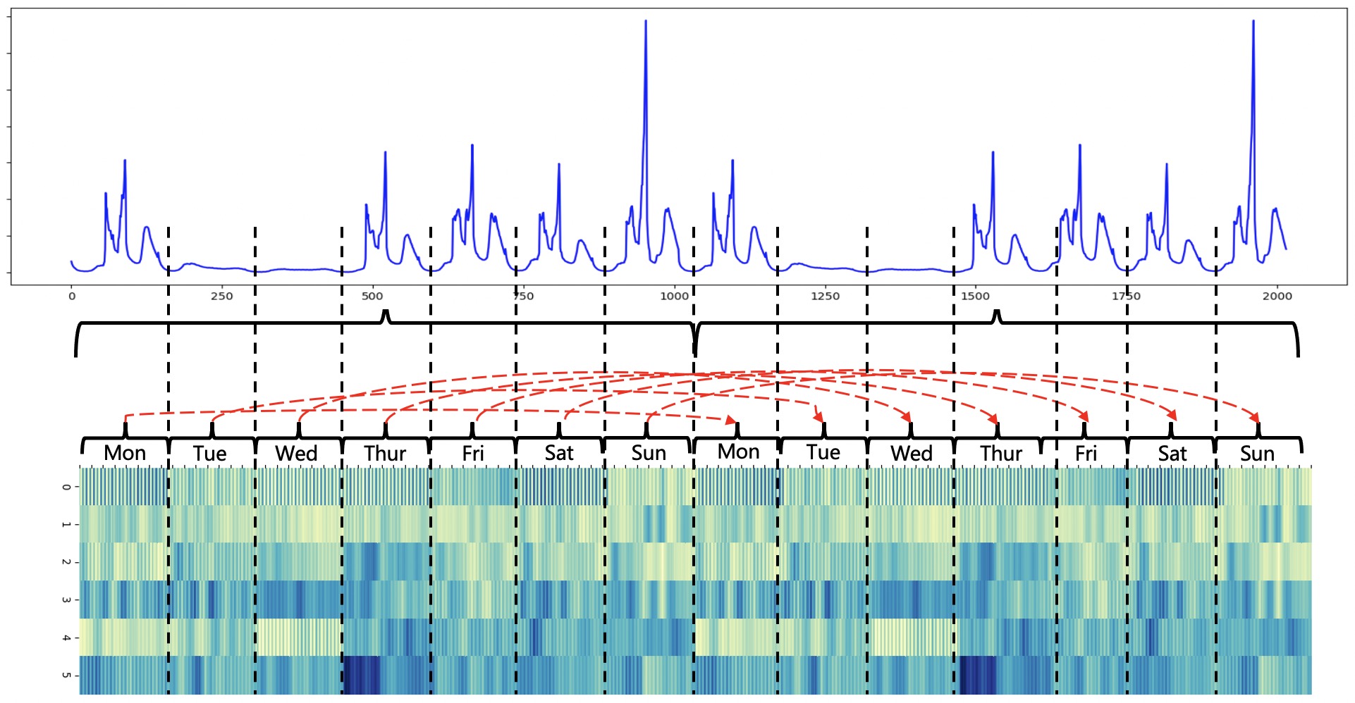
Figure 4: Visualization of TS representation of two weeks (every 10min). Changes in daily and weekly periods are clearly indicated.

In summary, benefiting from the powerful TS representation, we can capture workload TS of the high-frequency and non-stationary with various periods and complex long temporal dependencies. Furthermore, with the help of the self-attention-based fusion module, our model integrates long-term historical TS representations and short-term observations (nearby window) for better accuracy.

4.2.2 CPU-utilization and Workload Estimation

We take the target CPU utilization and id feature of the app as input, and output the per-Pod workload.

Baseline and Metrics. We conduct the performance comparison against state-of-the-art methods, including Linear Regression(LR), MLP, XGBoost(XGB), Gaussian Process(GP), Neural Process(NP) Garnelo et al. (2018). Please note that for LR, MLP, XGB, and GP, we build independent model for data in each scenario, but in contrast, a globally unified model is used for our approach (theoretically more difficult) and NP (generally considered a meta-learning method) is used to adapt to cross-scenario data, as detailed in Appendix B. We evaluate these experiments via MAE and RMSE.

Experiment Results. We run our experiment 5 times and reported the mean and standard deviation of the MAE and RMSE. Table 2 shows the performances of different approaches on the real-world datasets and we can observe that our proposed approach (Task-conditioned Bayesian Neural Regression) achieves all the best results, with significant improvements in accuracy (around 40%). Especially, by harnessing the power of the deep Bayesian method, our method characterizes the uncertainty between CPU utilization and workload, providing the upper and lower bounds of benefits and risks. Moreover, we generate different Bayesian model parameters for each set of application data by using a task-conditioned hypernetwork, which allows us to build a globally unified model across scenarios of data, greatly improving modeling efficiency compared with the above traditional methods.

Method	MAE	RMSE
Linear Regression	0.712(0.011)	1.315(0.023)
MLP	0.781(0.071)	1.152(0.533)
XGBoost	0.628(0.002)	1.240(0.004)
Gaussian Process	0.677(0.018)	1.271(0.136)
Neural Process	0.641(0.013)	1.275(0.375)
Our model	$\bm{0.365(0.005)}$	$\bm{0.799(0.016)}$

Table 2: The performance (lower is better) averaged over 5 runs.

4.2.3 Scaling Pods Decision

After finishing the above forecast and estimation, we obtain the total workload $y_{t}^{total}$ and upper and lower bounds of per-Pod workload $y_{t}^{{pod}}$. Therefore, according to Equation (1) above, we can obtain the decision range of the number of scaling Pods, where the upper bound corresponds to maximized benefits, and the lower bound corresponds to minimized risk.

Baseline and Metrics. We also conduct the performance comparison against state-of-the-art methods of autoscaling method with the Rule-based Autoscaling (Rule-based), Autopilot Rzadca et al. (2020), FIRM Qiu et al. (2020). We detail the above baselines in Appendix C.

We introduce relative resource consumption(RRC) as metrics to measure the performance of autoscaling, defined as:

$$RRC=c/c_{r}\mbox{ ,}$$ (6)

where $c$ is the Pod count allocated by the method for evaluation, and $c_{r}$ is the Pod count set by the baseline rule-based autoscaling method. Lower RRC indicates better efficiency (i.e., lower resource consumption).

Experiment Results. We run our experiment on 3000 online microservice applications to adjust Pods and report the RRC and scaling Pods count in Figure 5.

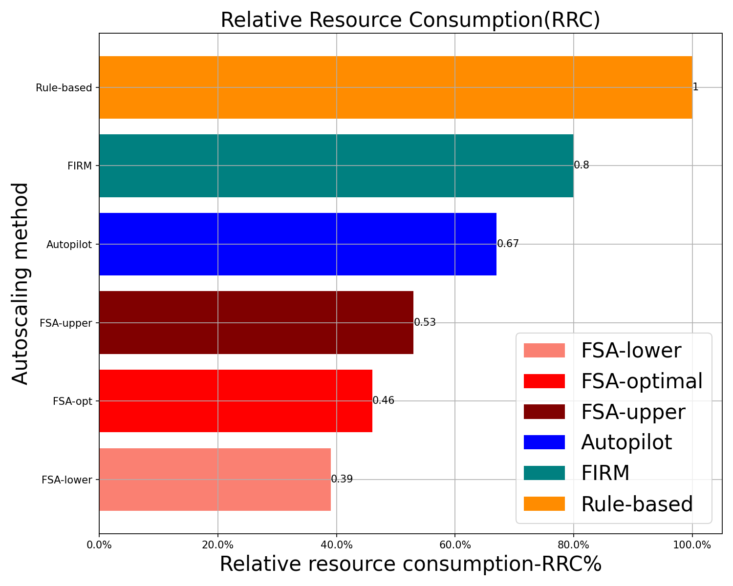
(a) Relative Resource Consumption

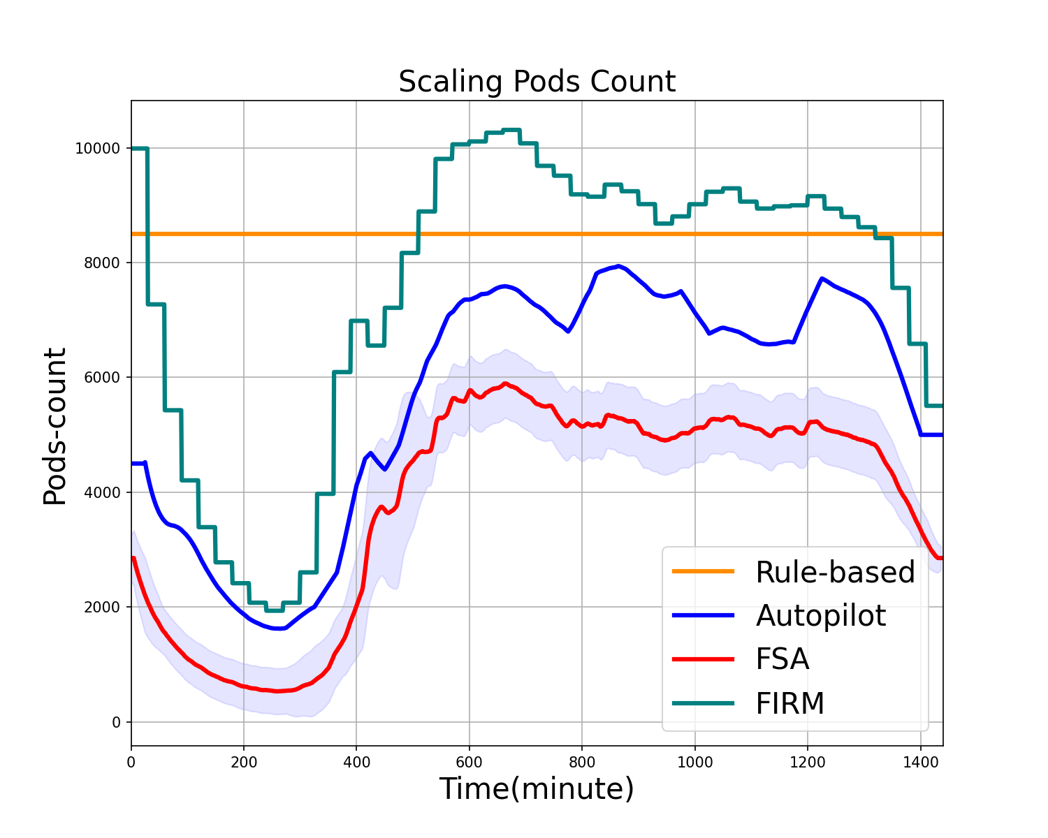
(b) Scaling Pods Count

Figure 5: The performance(lower is better) of different autoscaling approaches.

As seen in Figure 5, FSA demonstrates a significant performance improvement compared to other methods. On the premise of providing stable SLOs assurances and maintaining a target CPU utilization, FSA utilizes the least amount of resources. In particular, FSA provides the range of decisions for scaling Pods, including upper and lower bounds that represent benefit and risk respectively. We also can obtain the optimal value between the upper and lower bound according to service tolerance for response time (RT). Figure 5(b) shows the scaling Pods count by running each method in one day, which demonstrates the effectiveness and robustness of FSA. We characterize uncertainty in the decision-making process to provide upper and lower bounds for scaling, which allows our method to achieve stable SLOs assurances.

5 Deployment

Our approach is successfully deployed on the server cluster in our company’s data center, supporting the resource scheduling of more than 3000 online application services. As seen in Figure 6, we report the effectiveness of our approach in enhancing the sustainability of data centers over the past four years, resulting in greater resource efficiency and savings in electric energy. More details can be found in Appendix D.

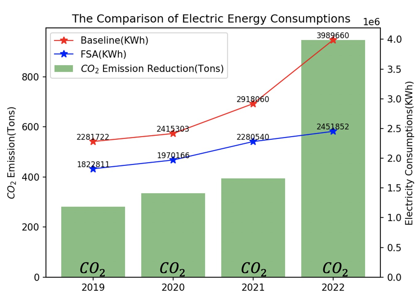
Figure 6: The Comparison of Electric Energy Consumptions. The red line represents the electricity consumption of baseline, and blue line is the electricity cost of FSA. The green histogram is the carbon emission reduction using FSA over the past four years.

FSA was applied in Double 11 shopping festivals over the past 4 years and according to the certification of China Environmental United Certification Center (CEC), the reductions of 282, 335, 394, 947 tons of carbon dioxide, respectively, (= savings of 459000, 545000, 640000, 1538000 kWh of electricity) were achieved during the shopping festivals.

6 Conclusion

In this paper, we proposed a Full Scaling Automation (FSA) mechanism to improve the energy efficiency and utilization of large-scale cloud computing clusters in data centers. The FSA mechanism utilizes forecasts of future workload demands to automatically adjust the resources available to meet the desired resource target level. Empirical tests on real-world data demonstrated the competitiveness of this method when compared to the state-of-the-art methods. Furthermore, the successful implementation of FSA in our own data center has reduced energy consumption and carbon emissions, marking an important step forward in our journey towards carbon neutrality by 2030.

Appendix A Workload TS Forecasting

A.1 Baseline

We conduct the performance comparison against state-of-the-art methods of TS forecasting below:

• N-BEATS: N-BEATS is an interpretable time series (TS) forecasting model, which is a deep neural architecture based on backward and forward residual links and very deep stack of fully-connected layers. The source code is available at https://github.com/philipperemy/n-beats.

• Transformer: Transformer is a recently popular method modeling sequences based on the self-attention mechanism. We use the native transformer implementation from PyTorch.

• LogTrans: LogTrans is a recently popular method modeling sequences based on the self-attention mechanism. We use the native transformer implementation from PyTorch. The source code is available at https://github.com/mlpotter/Transformer-Time-Series.

• Informer: Informer is a probsparse self-attention based model to enhance the prediction capacity in the long sequence TS forecasting problem, which validates the Transformer-like model’s potential value to capture individual long-range dependency between long sequence TS outputs and inputs. The source code is available at https://github. com/zhouhaoyi/Informer2020.

• Autoformer: Autoformer is a decomposition architecture by embedding the series decomposition block as an inner operator, which can progressively aggregate the long-term trend from intermediate predictions. The source code is available at https://github.com/thuml/Autoformer.

• Fedformer: Fedformer is a frequency-enhanced transformer model for long-term series forecasting which achieves state-of-the-art performance. The source code is available at https://github.com/thuml/Time-Series-Library.

• DeepAR: DeepAR is a univariate probabilistic forecasting model based on RNN, which is widely applied in real-world industrial applications. The code is from the Gluonts implementation on https://github.com/awslabs/gluon-ts.

A.2 Supplementary of Main Results

In order to compare performance of our method against state-of-the-art baselines, we plot the forecasting results from the test set of our dataset to qualitatively evaluate the predictions of different models in Figure 7, where we can observe that given the same input length, our model provides the best performance among all models. Particularly, during the peaks and troughs of the periods, our model demonstrates improved predictions. We conduct the ablation study on our model without representation and observe that incorporating TS representations significantly improves the prediction result. Moreover, we notice that our model with Multi-scale TS representation can accurately predict both the periodicity and long-term variation, i.e., our TS representation successfully characterizes long-term temporal dependencies across time periods. Furthermore, with the help of the self-attention-based fusion module, our model integrates long-term historical TS representations and short-term observations (nearby window) for better accuracy.

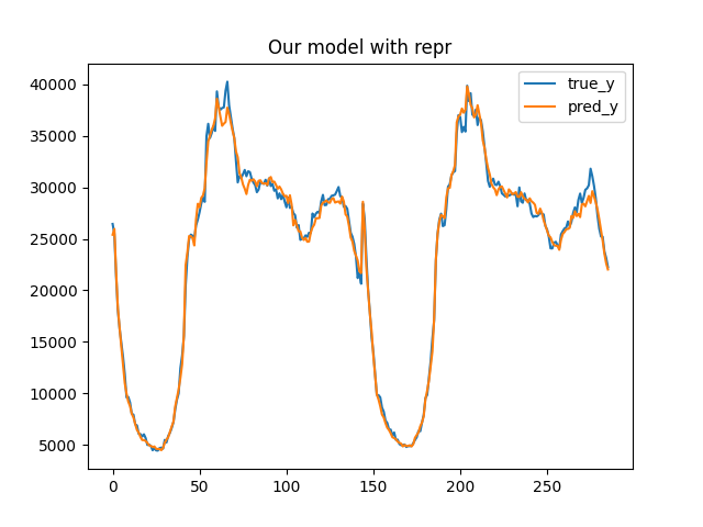
(a) Our model with repr.

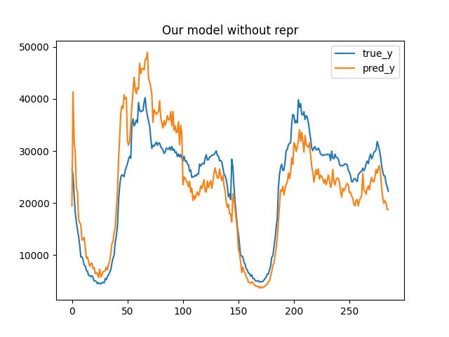
(b) Our model without repr.

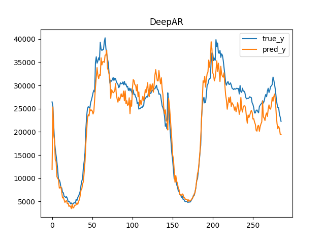
(c) DeepAR

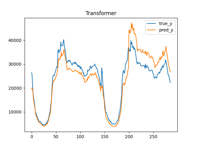
(d) Transformer

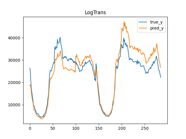
(e) LogTrans

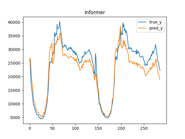
(f) Informer

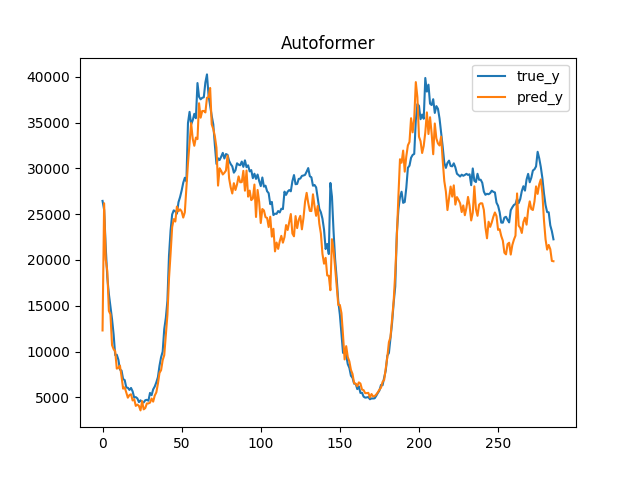
(g) Autoformer

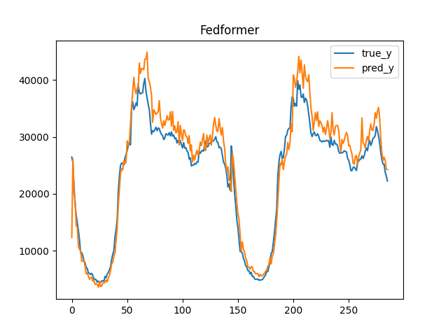
(h) Fedformer

Figure 7: Exemplar forecastings for workload TS. Blue lines are the ground truths and orange lines are the model predictions.

In Figure 8, we plot the visualization of the TS representations of different windows, and we can intuitively observe the changes in periods and trends from these representations. Even for TS that do not possess any observable periodic characteristic, our representation can still reveal its corresponding pattern of variations. This attests to the efficacy of our TS representation in capturing long-term temporal dependencies across time periods. Therefore, leveraging the Multi-scale TS representation in capturing the high-frequency and non-stationary workload TS is critical in achieving the improved performance of our model.

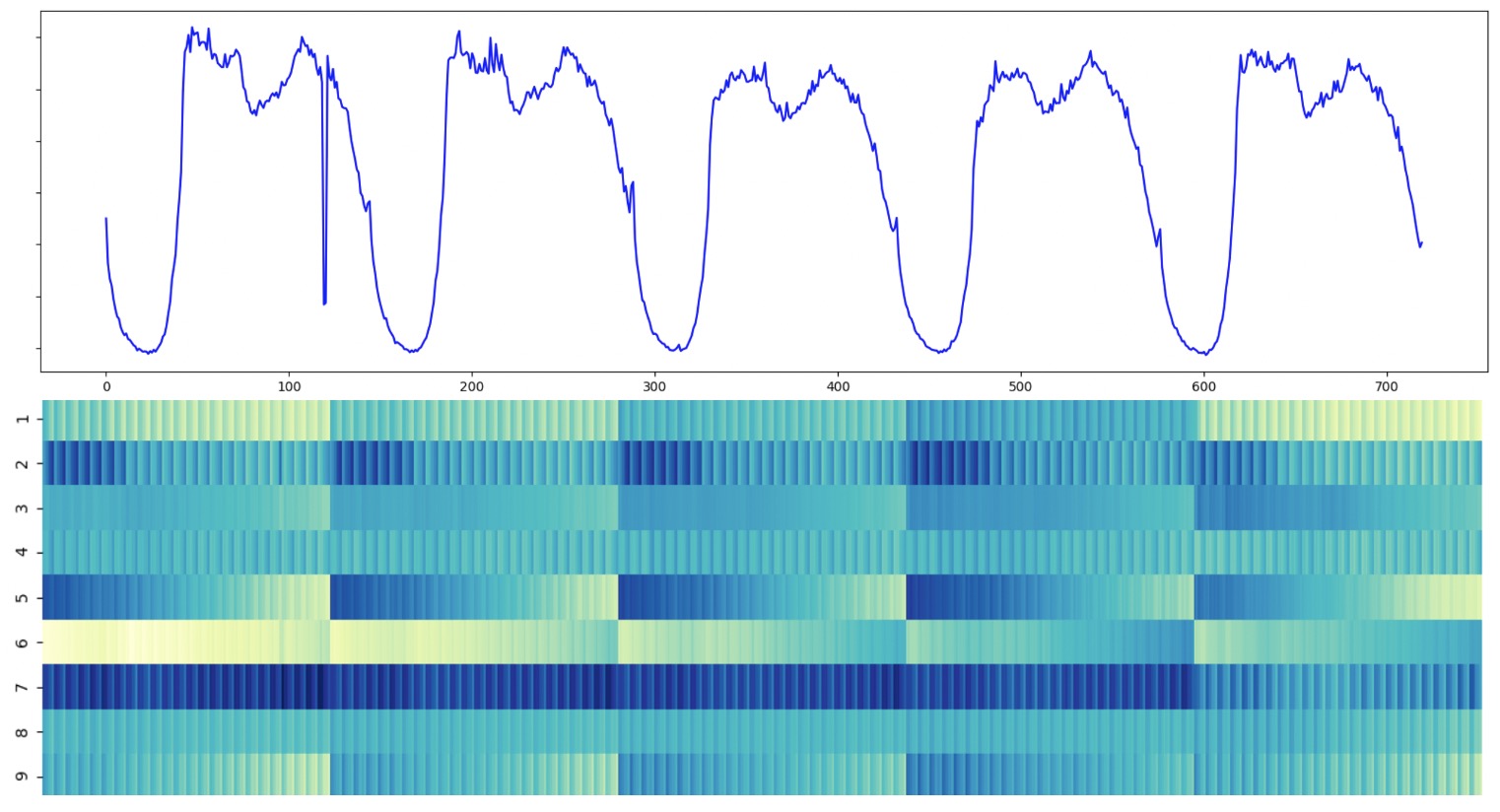
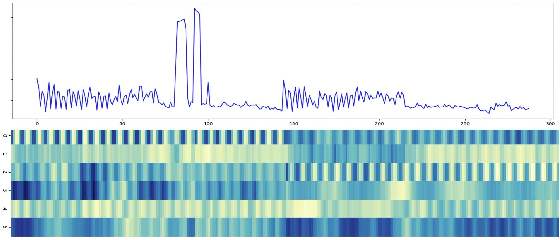
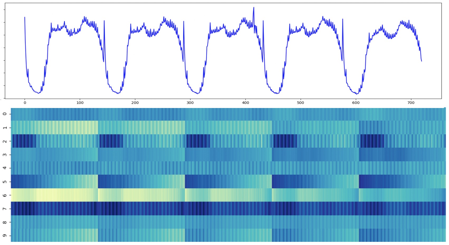
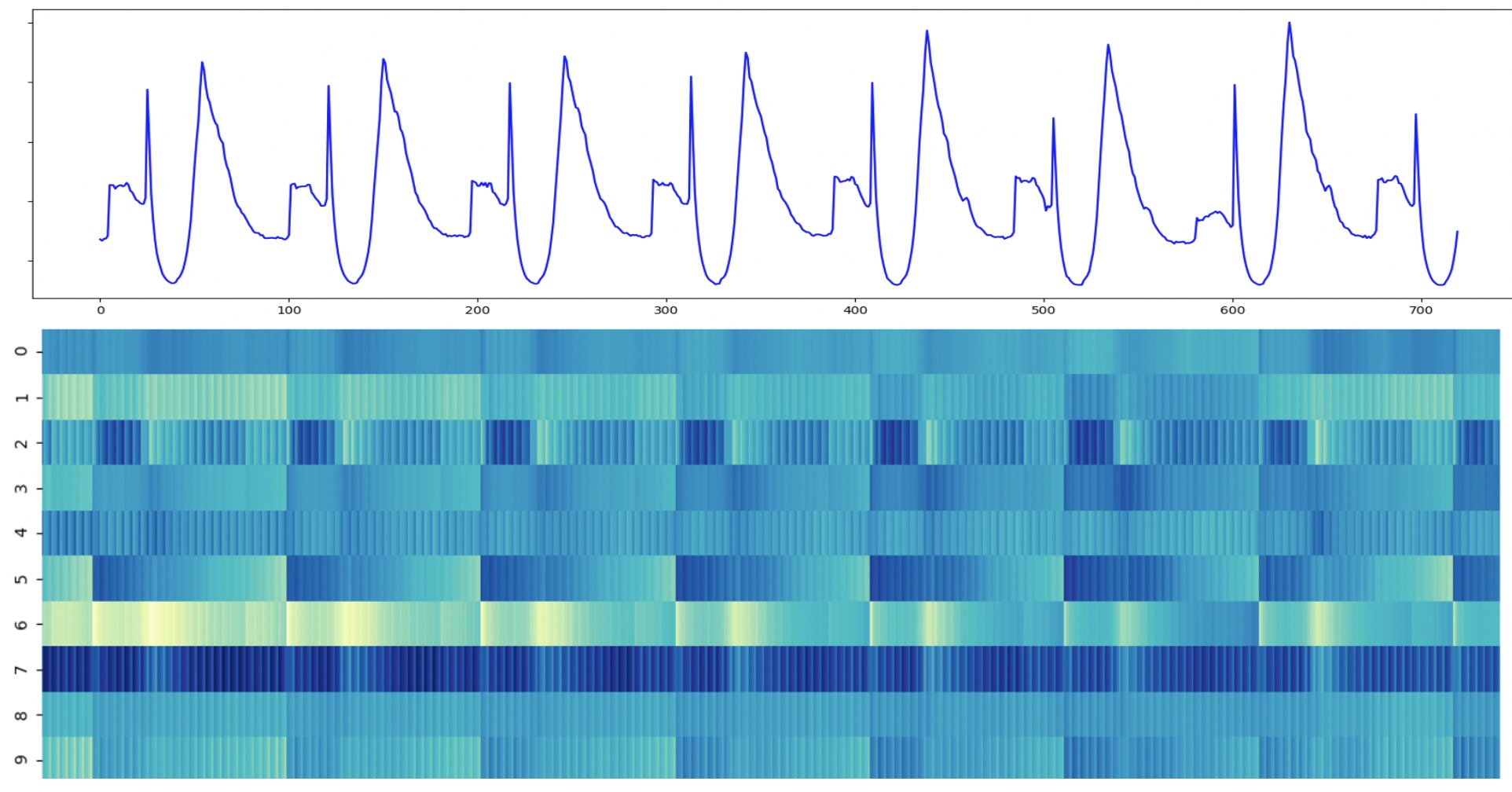
Figure 8: Visualization of TS representation of different windows of TS (every 10 minutes).

Appendix B CPU-utilization and Workload Estimation

B.1 Baseline

We conduct the performance comparison against state-of-the-art methods of regression below:

• Linear Regression: Linear Regression (LR) is a linear approach for modeling the relationship between a scalar response and one or more explanatory variables (also known as dependent and independent variables). The source code is available at https://github.com/scikit-learn/scikit-learn.

• Multilayer Perceptron: Multilayer Perceptron (MLP) is an artificial neural network composed of multiple layers of neurons with a nonlinear activation function. MLPs are commonly used for classification and regression tasks. We implement MLP using PyTorch.

• XGBoost: XGBoost (XGB) is a supervised learning algorithm based on the powerful gradient boosting framework that is designed to predict numerical values from a set of input data. It uses a gradient descent approach to optimize differentiable loss functions and is capable of dealing with large datasets. The source code is available at https://github.com/dmlc/xgboost .

• Gaussian Process: Gaussian Process (GP) is a probabilistic model that makes predictions based on a set of data points. It is a supervised learning algorithm that makes predictions by constructing a probability distribution over the space of potential outcomes. The source code is available at https://github.com/scikit-learn/scikit-learn.

• Neural process: Neural Process (NP) uses a combination of Bayesian neural networks and Gaussian processes to construct a probability distribution over the space of potential outcomes. NP is typically used for regression tasks as it allows for flexible and powerful modeling of the data. The source code is available at https://github.com/deepmind/neural-processes.

B.2 Supplementary of Main Results

We plot our model estimation results in Figure 9. We take the target CPU utilization and id feature of the app as input and output the per-Pod workload.

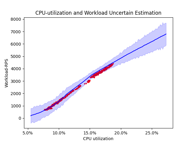
Figure 9: Visualization of CPU-utilization and workload estimation. Blue lines are the mean of estimation. Red scattered points are the ground truths. Purple area is the confidence interval.

As seen in Figure 9, it is perceptible that our method not only yields accurate estimations, but also provides confidence intervals to bestow insight into the uncertainties of the outcomes. In practice, affected by various aspects of the servers (such as temperature), the uncertainty of the correlation between CPU utilization and workload needs to be modeled in the decision-making process to balance between benefits and risks. In particular, benefiting from harnessing the power of the deep Bayesian method, our model provides upper and lower bounds on the estimations to facilitate the decision of Pod-scaling.

Appendix C Scaling Pods Decision

C.1 Baseline

We conduct the performance comparison against state-of-the-art methods of autoscaling below:

• Autopilot: Google proposed Autopilot, a workload-based autoscaling method, which identifies the most appropriate resource configuration by comparing the current time window to relevant historical time windows. We implement Autopilot in accordance with the details in its public paper.

• FIRM: FIRM is a Service Level Objectives (SLOs)-based autoscaling method, designed to address the problem of dynamic resource adjustment in a cloud environment through continuous feedback and learning. Specifically, FIRM utilizes a support vector machine (SVM)-based anomaly detection algorithm to identify applications with an abnormal response time (RT), and utilizes reinforcement learning (RL) algorithms to adjust multiple resources accordingly. We implement FIRM from https://gitlab.engr.illinois.edu/DEPEND/firm.

• Rule-based Autoscaling: Rule-based Autoscaling provides a means of leveraging monitored performance metrics and expert-defined rules to dynamically adjust the quantity of Pods associated with a particular microservice.

C.2 Supplementary of Main Results

We introduce relative resource consumption (RRC) as metrics to measure the performance of autoscaling, defined as:

$$RRC=c/c_{r}\mbox{ ,}$$

where $c$ is the Pod count allocated by the method for evaluation, and $c_{r}$ is the Pod count set by the baseline rule-based autoscaling method. Lower RRC indicates better efficiency (i.e., lower resource consumption).

We run our experiment on 3000 online microservice applications to adjust Pods and report the relative resource consumption (RRC) and scaling Pods count in Figure 10.

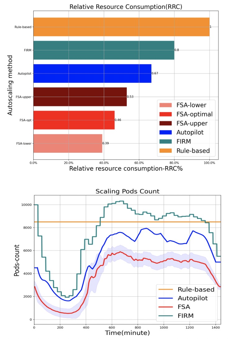
Figure 10: The performance (lower is better) of different autoscaling approaches.

Figure 5 shows that FSA outperforms other methods significantly. FSA is the most resource-efficient, ensuring stable SLOs assurances and maintaining CPU utilization at its target level. Especially, FSA offers a variety of choices to scale Pods (providing upper and lower bound), from ones with the highest potential benefit to those with the least risk. It is possible to ascertain the optimal number of scaling Pods between the upper and lower bound in accordance with service tolerance for response time (RT). The scaling Pods count for each method run in one day, as illustrated in the bottom half of Figure 5, attests to the effectiveness and robustness of FSA.

Appendix D Deployment

D.1 Performance in the Production Environment

The FSA has already been deployed in the production environment of our company’s data center, supporting the resource scheduling of more than 3000 online application services. Figure 5 shows the performance in the production environment including workload TS, CPU utilization, and scaling Pods count. The green frame indicates the comparison of servers’ indicators under the same workload before and after enabling FSA. It is evident that, with the same workload, the enabling of FSA results in a significant improvement of CPU utilization in the cluster and a substantial decrease in the number of Pods (from 1500 to fewer than 500). As a result, electricity consumption or carbon emissions is effectively reduced, which is the key to promoting sustainable development for green data centers.

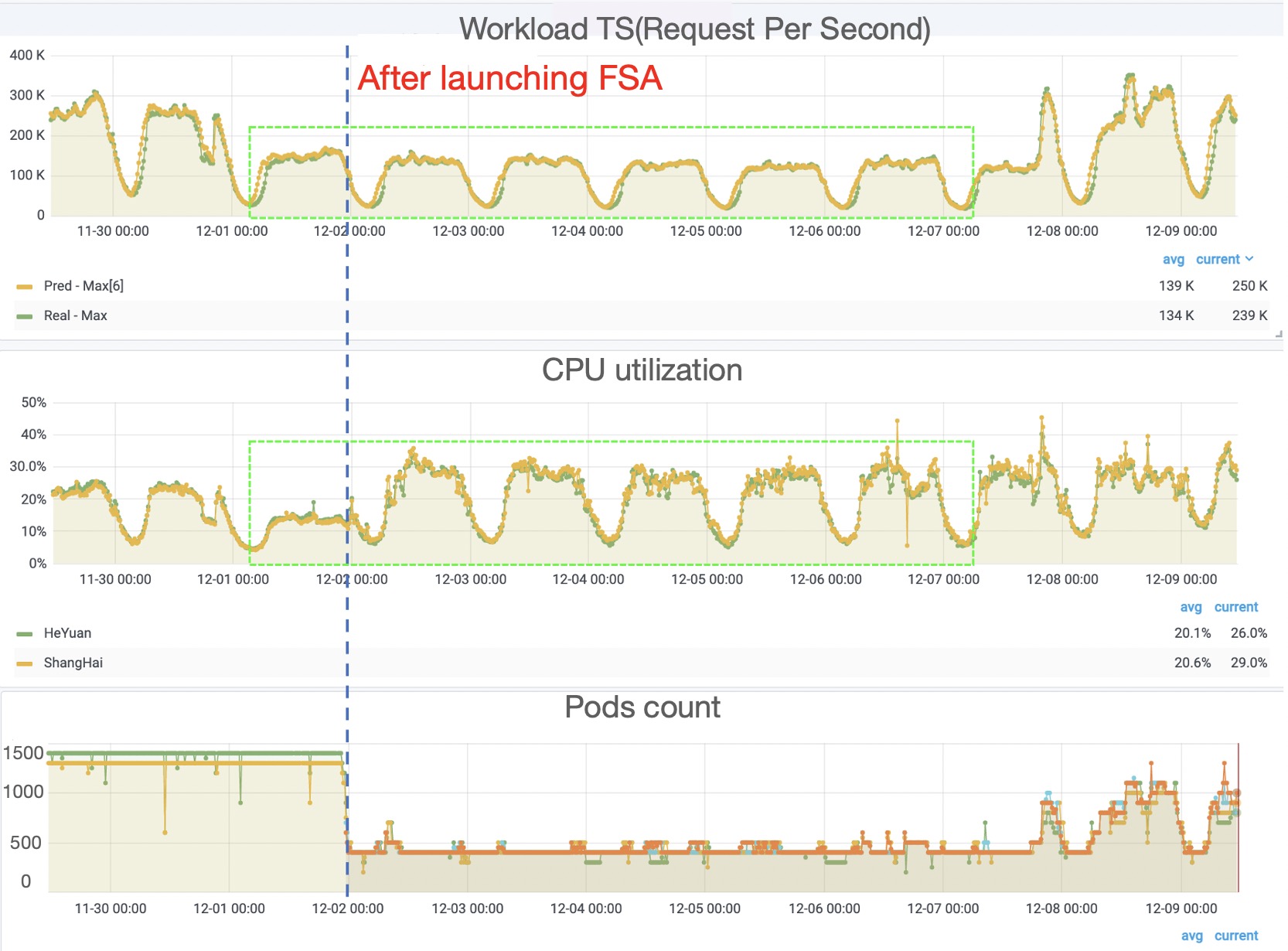
Figure 11: The performance of Autoscaling deployed in the production environment. Blue vertical dotted line indicates the launch of FSA. Green frame highlights the comparison of the metrics under the same workload before and after enabling FSA.

The nighttime CPU utilization in the figure is reduced due to the requirement to preserve a predetermined number of Pods from deallocation (for risk avoidance considerations). In fact, our method can consistently maintain the desired target CPU utilization by predictive scaling.

D.2 Measurement of Electricity Consumption

We can calculate the electricity consumption as follows:

$$cost=n*p*u*d\mbox{ ,}$$ (7)

where $n$ is the number of servers equipment used, $p$ is the average power of servers, $u$ is the power usage effectiveness (PUE ) in the data center, and $d$ is the running duration of the servers. Power saving can also be easily converted to carbon reduction. In Figure 12, we report the above running metric of server clusters in our data center over the past 4 years. We can intuitively see that by using FSA for autoscaling, the number of required servers is greatly reduced, while the CPU utilization is significantly improved. Despite the fact that server power consumption has increased due to improve utilization of resources, we have managed to make a substantial decrease in the data center’s PUE.

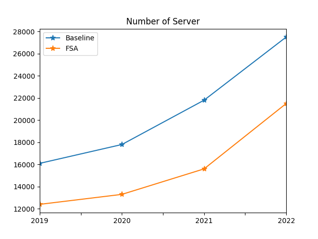
(a) Number of Servers

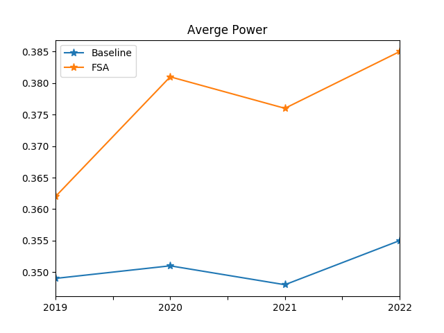
(b) Average Power of Servers

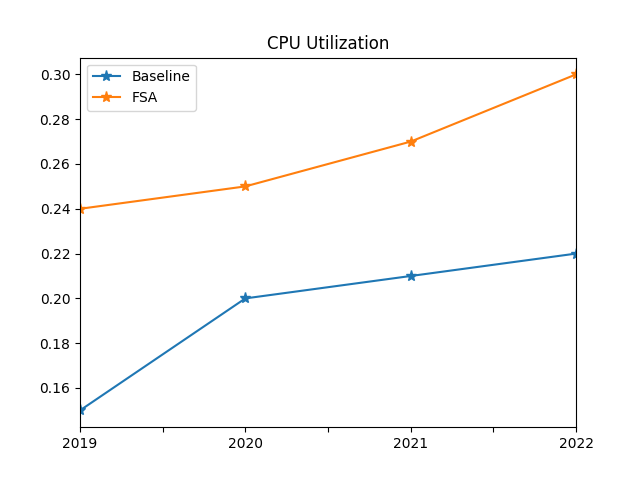
(c) CPU Utilization of Servers

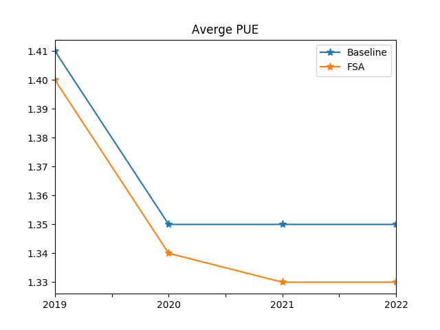
(d) Average PUE of Data Center

Figure 12: The running metric of server clusters in our data center over the past 4 years.

Appendix E Sustainable Development in Our Company

Our company stands as the premier provider of payment technology worldwide, with server clusters powered by in excess of 9 million CPU cores, and ranking among the top ten in the world in terms of server scale. We introduced a comprehensive ESG (Environmental, Social, and Governance) framework to upgrade our sustainability governance system. This framework will guide our value creation and sustainable development in the future. These initiatives showcase our commitments and actions for a better future.

In light of this, we are devoted to furthering the use of AI technology to foster sustainable development. This inspired us to develop a technology known as Green Computing, which can significantly optimize resource utilization by efficiently scheduling large-scale server clusters, and thus decreasing energy usage and attaining the sustainable development goal of cutting down on carbon emissions.

Moreover, we are working in conjunction with China Environmental United Certification Center (CEC) to map the decreased energy consumption to the equivalent carbon emissions in the data center. CEC is a non-profit and autonomous third-party organization that offers comprehensive certification and service solutions for environmental protection, energy conservation, and low-carbon sectors in China.

Over the past four years, the extensive utilization of green computing technology in our top-ten data centers worldwide has cumulatively resulted in the reduction of more than 100,000 tons of carbon dioxide emissions. This makes a significant contribution to our company’s goal of achieving carbon neutrality by 2030. We are looking forward to advance the sustainable development of green data centers across the industry by disclosing our patents, technologies, and papers, in order to accomplish the ambition of a global zero-carbon society in the future.

References

- Abdullah et al. (2020) Muhammad Abdullah, Waheed Iqbal, Josep Lluis Berral, Jorda Polo, and David Carrera. Burst-aware predictive autoscaling for containerized microservices. IEEE Transactions on Services Computing, 15(3):1448–1460, 2020.
- Bishop and Nasrabadi (2006) Christopher M Bishop and Nasser M Nasrabadi. Pattern recognition and machine learning, volume 4. Springer, 2006.
- Blundell et al. (2015) Charles Blundell, Julien Cornebise, Koray Kavukcuoglu, and Daan Wierstra. Weight uncertainty in neural network. In International conference on machine learning, pages 1613–1622. PMLR, 2015.
- Campbell (2017) Della Anne Campbell. An update on the united nations millennium development goals. Journal of Obstetric, Gynecologic & Neonatal Nursing, 46(3):e48–e55, 2017.
- climatiq.io (2021) climatiq.io. Measuring greenhouse gas emissions in data centres: the environmental impact of cloud computing, 2021.
- Eldele et al. (2021) Emadeldeen Eldele, Mohamed Ragab, Zhenghua Chen, Min Wu, Chee Keong Kwoh, Xiaoli Li, and Cuntai Guan. Time-series representation learning via temporal and contextual contrasting. arXiv preprint arXiv:2106.14112, 2021.
- Garnelo et al. (2018) Marta Garnelo, Jonathan Schwarz, Dan Rosenbaum, Fabio Viola, Danilo J Rezende, SM Eslami, and Yee Whye Teh. Neural processes. arXiv preprint arXiv:1807.01622, 2018.
- He et al. (2022) Yun He, Steven Zheng, Yi Tay, Jai Gupta, Yu Du, Vamsi Aribandi, Zhe Zhao, YaGuang Li, Zhao Chen, Donald Metzler, et al. Hyperprompt: Prompt-based task-conditioning of transformers. In International Conference on Machine Learning, pages 8678–8690. PMLR, 2022.
- Kingma and Welling (2013) Diederik P Kingma and Max Welling. Auto-encoding variational bayes. arXiv preprint arXiv:1312.6114, 2013.
- Krieger et al. (2017) Michael T Krieger, Oscar Torreno, Oswaldo Trelles, and Dieter Kranzlmüller. Building an open source cloud environment with auto-scaling resources for executing bioinformatics and biomedical workflows. Future Generation Computer Systems, 67:329–340, 2017.
- Mahabadi et al. (2021) Rabeeh Karimi Mahabadi, Sebastian Ruder, Mostafa Dehghani, and James Henderson. Parameter-efficient multi-task fine-tuning for transformers via shared hypernetworks. arXiv preprint arXiv:2106.04489, 2021.
- Nguyen et al. (2020) Thanh-Tung Nguyen, Yu-Jin Yeom, Taehong Kim, Dae-Heon Park, and Sehan Kim. Horizontal pod autoscaling in kubernetes for elastic container orchestration. Sensors, 20(16):4621, 2020.
- Oreshkin et al. (2019) Boris N Oreshkin, Dmitri Carpov, Nicolas Chapados, and Yoshua Bengio. N-beats: Neural basis expansion analysis for interpretable time series forecasting. arXiv preprint arXiv:1905.10437, 2019.
- Qiu et al. (2020) Haoran Qiu, Subho S Banerjee, Saurabh Jha, Zbigniew T Kalbarczyk, and Ravishankar K Iyer. FIRM: An intelligent fine-grained resource management framework for SLO-Oriented microservices. In 14th USENIX Symposium on Operating Systems Design and Implementation (OSDI 20), pages 805–825, 2020.
- Rzadca et al. (2020) Krzysztof Rzadca, Pawel Findeisen, Jacek Swiderski, Przemyslaw Zych, Przemyslaw Broniek, Jarek Kusmierek, Pawel Nowak, Beata Strack, Piotr Witusowski, Steven Hand, et al. Autopilot: workload autoscaling at google. In Proceedings of the Fifteenth European Conference on Computer Systems, pages 1–16, 2020.
- Salinas et al. (2020) David Salinas, Valentin Flunkert, Jan Gasthaus, and Tim Januschowski. Deepar: Probabilistic forecasting with autoregressive recurrent networks. International Journal of Forecasting, 36(3):1181–1191, 2020.
- UN (2021) UN. United nations climate conference: Sustainability in data centres, 2021.
- Woo et al. (2022) Gerald Woo, Chenghao Liu, Doyen Sahoo, Akshat Kumar, and Steven Hoi. Cost: Contrastive learning of disentangled seasonal-trend representations for time series forecasting. arXiv preprint arXiv:2202.01575, 2022.
- Yue et al. (2022) Zhihan Yue, Yujing Wang, Juanyong Duan, Tianmeng Yang, Congrui Huang, Yunhai Tong, and Bixiong Xu. Ts2vec: Towards universal representation of time series. In Proceedings of the AAAI Conference on Artificial Intelligence, volume 36, pages 8980–8987, 2022.
- Zhou et al. (2021) Haoyi Zhou, Shanghang Zhang, Jieqi Peng, Shuai Zhang, Jianxin Li, Hui Xiong, and Wancai Zhang. Informer: Beyond efficient transformer for long sequence time-series forecasting. In Proceedings of AAAI, 2021.