Scaling of Piecewise Deterministic Monte Carlo for Anisotropic Targets

Abstract

Piecewise deterministic Markov processes (PDMPs) are a type of continuous-time Markov process that combine deterministic flows with jumps. Recently, PDMPs have garnered attention within the Monte Carlo community as a potential alternative to traditional Markov chain Monte Carlo (MCMC) methods. The Zig-Zag sampler and the Bouncy particle sampler are commonly used examples of the PDMP methodology which have also yielded impressive theoretical properties, but little is known about their robustness to extreme dependence or isotropy of the target density. It turns out that PDMPs may suffer from poor mixing due to anisotropy and this paper investigates this effect in detail in the stylised but important Gaussian case. To this end, we employ a multi-scale analysis framework in this paper. Our results show that when the Gaussian target distribution has two scales, of order $1$ and $\epsilon$, the computational cost of the Bouncy particle sampler is of order $\epsilon^{-1}$, and the computational cost of the Zig-Zag sampler is either $\epsilon^{-1}$ or $\epsilon^{-2}$, depending on the target distribution. In comparison, the cost of the traditional MCMC methods such as RWM or MALA is of order $\epsilon^{-2}$, at least when the dimensionality of the small component is more than $1$. Therefore, there is a robustness advantage to using PDMPs in this context.

1 Introduction

Piecewise deterministic Markov processes (PDMPs) are continuous-time non-reversible Markov processes driven by deterministic flows and jumps. Recently, PDMPs have attracted attention of the Monte Carlo community as a possible alternative to traditional Markov chain Monte Carlo methods. The Zig-Zag sampler [5] and the Bouncy particle sampler [9] are commonly used examples of the PDMP methodology which have also yielded impressive theoretical properties, for example in high-dimensional contexts [11, 1, 6], and in the context of MCMC with large data sets [5].

It is well-known that all MCMCs suffer from deterioration of mixing properties in the context of anisotropy of the target distribution. For example the mixing of random walk Metropolis, Metropolis-Adjusted Langevin and Hamiltonian schemes can all become arbitrarily bad in any given problem for increasingly inappropriately scaled proposal distributions (see for example the studies in [23, 24, 25, 3, 4, 15]). Meanwhile the Gibbs sampler is known to perform poorly in the context of highly correlated target distributions, see for example [27, 28]. In principle these problems can be overcome using preconditioning (a priori reparameterisations of the state space), often carried out using adaptive MCMC [2, 26]. However effective preconditioning can be very difficult in higher-dimensional problems. Therefore it is important to understand the extent of this deterioration of mixing in the face of anisotropy or dependence.

PDMPs can also suffer poor mixing due to anisotropy and this paper will study this effect in detail in the stylised but important Gaussian case. In principle, continuous time processes are well-suited to this problem because they do not require a rejection scheme, unlike traditional MCMC methods which suffer from a scaling issue. However, this does not guarantee that the processes will be effective for this problem. Even if the process mixes well, it may require a large number of jumps, resulting in high computational cost. To understand this quantitatively, it is important to determine the influence that anisotropies in the target distribution have on the speed convergence to equilibrium.

However, for continuous-time processes a further consideration relevant to the computational efficiency of an algorithm involves some measure of the computational expense expended per unit stochastic process time. It is difficult to be precise about how to measure this in general. Here we will use a commonly adopted surrogate: the number of jumps per unit time. Effectively this assumes that we have access to an efficient implementation scheme for our PDMP via an appropriate Poisson thinning scheme, which is not always available in practice.

This quantification of the computational cost can be achieved by the scaling analysis which first appeared in [23] in the literature under mathematically formal argument. In this paper, we follow [4] that studied the random walk Metropolis algorithm for anisotropic target distributions. To avoid technical difficulties, they considered a simple target distribution with both small and large-scale components, where these two components are conditionally independent. The scale of the noise of the algorithm must be appropriately chosen in advance, otherwise, the algorithm will be frozen. On the other hand, the piecewise deterministic Markov processes naturally fit the scale without artificial parameter tuning. However, from a theoretical point of view, this makes the analysis complicated since the process changes its dynamics depending on the target distribution. Therefore, we study a simple Gaussian example and identify the factors that change the dynamics for a better understanding of the processes for anisotropic target distributions.

The main contributions of this paper are thus

1. We give a theoretical and rigorous study of the robustness of Zig-Zag and BPS algorithms in the case of increasingly extreme isotropy (where one component is scaled by a factor $\epsilon$ which converges to $0$ in the limit). The results give weak convergence results to characterise the limiting dynamics of the slow component in the extreme isotropy limit.

2. For the Zig-Zag, we see that, unless the slow component is either (a) perfectly aligned with one of the possible velocity directions, or (b) independent of the fast component, the limiting behaviour is a reversible Ornstein–Uhlenbeck process (4.4) as presented in Theorem 3.2, and which mixes in time $O(\epsilon^{-1})$ but for which $O(\epsilon^{-1})$ switches are required by Theorem 3.3 leading to a complexity which is $O(\epsilon^{-2})$.

3. For BPS, the limiting behaviour is a deterministic dynamical system for which we can explicitly write down its generating ODE (5.25) as presented in Theorem 3.4. Mixing is $O(1)$ and the number of switches required for this is $O(\epsilon^{-1})$ switches by Theorem 3.5 leading to a complexity which is $O(\epsilon^{-1})$.

The paper is organised as follows. In Section 2 we explore the problem in a 2-dimensional setting where we can easily illustrate and motivate our results. Here we describe the limiting processes using the homogenisation and averaging techniques of [22]. Section 3 then describes our main results in detail and signposts the proofs. Sections 4 and 5 then gives the detailed proofs for the Zig-Zag and BPS respectively, supported by technical material from the Appendix A. A final discussion is given in Section 6.

Recent work [1] provides $L^{2}$-exponential convergence for general target distributions, identifying the exponential rate even in high-dimensional scenarios. Their results can also be applied to anisotropic target distributions. However, it is worth noting that it is currently unclear how to achieve the same rate for anisotropic target distributions as described above.

2 Exhibit of main results in the two-dimensional case

To better understand our result, we first consider the two-dimensional case, which is easier to interpret than the general result. Consider the situation of a two-dimensional Gaussian target distribution with one large and one small component. Indeed, let $\Sigma^{\epsilon}=U^{\top}(\Lambda^{\epsilon})^{2}U$, where

$$U=\begin{pmatrix}\cos\theta&-\sin\theta\\ \sin\theta&\cos\theta\end{pmatrix}\quad\text{and}\quad\Lambda^{\epsilon}=\begin{pmatrix}1&0\\ 0&\epsilon\end{pmatrix}.$$ (2.1)

We will show that the Markov processes of the Zig-Zag sampler and the Bouncy particle sampler converges to limit processes as $\epsilon\rightarrow 0$ if we choose a correct scaling in space and time.

To illustrate the impact of $\epsilon$, we will use a reparametrised variable for our scaling analysis:

$$y=(\Lambda^{\epsilon})^{-1}Ux.$$ (2.2)

By this variable scaling, the invariant distribution of the Markov semigroup corresponding to $\xi=(y,v)$ is $\mu=\mathcal{N}_{d}(0,I_{d})\otimes\mathcal{U}(\{-1,+1\}^{d})$ for the Zig-Zag sampler, and $\mu=\mathcal{N}_{d}(0,I_{d})\otimes\mathcal{N}_{d}(0,I_{d})$ for the Bouncy Particle Sampler.

2.1 The Zig-Zag sampler in the two dimensional case

The Markov generator of the two-dimensional Zig-Zag sampler with reparametrisation is

$$\mathcal{L}^{\epsilon}f(y,v) =(v_{1}\cos\theta-v_{2}\sin\theta)\partial_{y_{1}}f(y,v)$$ (2.3)

$$\quad+\epsilon^{-1}(v_{1}\sin\theta+v_{2}\cos\theta)\partial_{y_{2}}f(y,v)$$

$$\quad+\left(v_{1}(y_{1}\cos\theta+\epsilon^{-1}y_{2}\sin\theta)\right)_{+}~{}(\mathcal{F}_{1}-\operatorname{id})f(y,v)$$

$$\quad+\left(v_{2}(-y_{1}\sin\theta+\epsilon^{-1}y_{2}\cos\theta)\right)_{+}~{}(\mathcal{F}_{2}-\operatorname{id})f(y,v),$$

where $\mathcal{F}_{i}f(y,v)=f(y,F_{i}(v))$ and $F_{i}$ represents the operation that flips the sign of the $i$-th component. Figure 1 displays the trajectories of the Zig-Zag sampler in a two-dimensional scenario, with $\theta=0,\pi/6$ and $\pi/4$ and $\epsilon=0.01$.

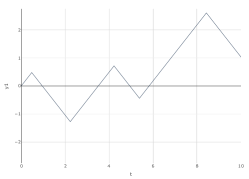
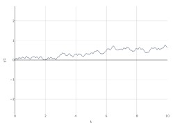
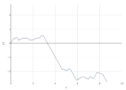
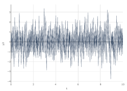
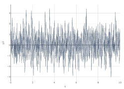
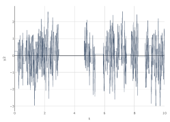
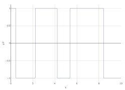
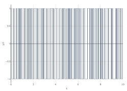
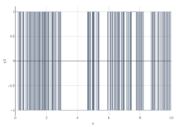
Figure 1: Paths of $y_{1}$ for $\theta=0$ (left), $\theta=\pi/6$ (centre), and $\theta=\pi/4$ (right), and $y_{1}$ ($1$st row), $y_{2}$ ($2$nd row) and $v_{1},v_{2}$ ($3$rd and $4$th rows) of the Zig-Zag sampler where $\epsilon=0.01$.

Our first observation from Figure 1 is that the process of $(y_{2},v_{1},v_{2})$ exhibits good mixing, whereas the process of $y_{1}$ does not. This result is expected, as the terms in the expression for $\mathcal{L}^{\epsilon}$ that correspond to the dynamics of $(y_{2},v_{1},v_{2})$ are proportional to $\epsilon^{-1}$, whereas the dynamics of $y_{1}$ are of order $O(1)$. When $\epsilon$ is sufficiently small, the dynamics of $(y_{2},v_{1},v_{2})$ are described by the operator $\mathcal{L}_{0}$, which is derived from $\mathcal{L}^{\epsilon}$ by retaining only terms proportional to $\varepsilon^{-1}$:

$$\mathcal{L}_{0}f(y,v) =(v_{1}\sin\theta+v_{2}\cos\theta)~{}\partial_{y_{2}}f(y,v)$$

$$\quad+\left(v_{1}y_{2}\sin\theta\right)_{+}~{}(\mathcal{F}_{1}-\operatorname{id})f(y,v)+\left(v_{2}y_{2}\cos\theta\right)_{+}~{}(\mathcal{F}_{2}-\operatorname{id})f(y,v).$$

Our second observation is that the Zig-Zag process corresponding to $y_{1}$ generally demonstrates diffusive behaviour, except in some specific situations, which correspond to the figures on the left and right in Figure 1. The behaviour in these exceptional scenarios will be discussed in Section 2.1.1. For the time being, we make the following assumption.

Assumption 2.1.

$\theta\in[0,2\pi)$ but $\theta\neq n\pi/4\ (n=0,\ldots,7)$.

To elucidate the asymptotic behaviour, the solution of the Poisson equation plays a crucial role, as it enables the separation of the fast dynamics associated with the $y_{2}$ process and the slow dynamics associated with the $y_{1}$ process. Let $\chi(y_{2},v)$ denote the solution to the Poisson equation

$$\mathcal{L}_{0}\chi(y_{2},v)=-(v_{1}\cos\theta-v_{2}\sin\theta).$$ (2.4)

Let $\Omega=-2\mu(\chi~{}\mathcal{L}_{0}\chi)$ which can be shown to admit the expression

$$\Omega=\begin{cases}\dfrac{8}{\sqrt{\pi}}\dfrac{\operatorname{arctanh}\sqrt{|\tan\theta|}}{(1+|\sin 2\theta|)\sqrt{|\sin 2\theta|}}+\dfrac{\sqrt{2\pi}}{|\sin\theta|(1+|\sin 2\theta|)}&\mathrm{if}\ |\sin\theta|<|\cos\theta|\\ \vspace{1px}\\ \dfrac{8}{\sqrt{\pi}}\dfrac{\operatorname{arctanh}\sqrt{1/|\tan\theta|}}{(1+|\sin 2\theta|)\sqrt{|\sin 2\theta|}}+\dfrac{\sqrt{2\pi}}{|\cos\theta|(1+|\sin 2\theta|)}&\mathrm{if}\ |\sin\theta|>|\cos\theta|\end{cases}$$ (2.5)

for $\theta\neq n\pi/4\ (n=0,\ldots,7)$. See Figure 2. The expression of $\chi$, along with the derivation of $\Omega$, can be found in Appendix A.1.

Let $y_{1}^{\epsilon}(t)$ be the $y_{1}$-coordinate of the Zig-Zag sampler process. The following is the formal statement of our second observation. Let $\mathbb{D}[0,T]$ be the space of càdlàg processes on $[0,T]$ equipped with the Skorokhod topology.

Theorem 2.2.

Under Assumption 2.1, and when the process is stationary, the $\epsilon^{-1}$-time scaled process $y_{1}^{\epsilon}(\epsilon^{-1}t)$ converges weakly in $\mathbb{D}[0,T]$ for any $T>0$ to the Ornstein–Uhlenbeck process

$$\mathrm{d}X_{t}=-\frac{\Omega}{2}~{}X_{t}\mathrm{d}t+\Omega^{1/2}\mathrm{d}W_{t}$$

where $W_{t}$ is the one-dimensional standard Wiener process.

The convergence of this process is a consequence of the multi-dimensional result established in Theorem 3.2. Figure 3 shows that the theory agrees well with a numerical experiment.

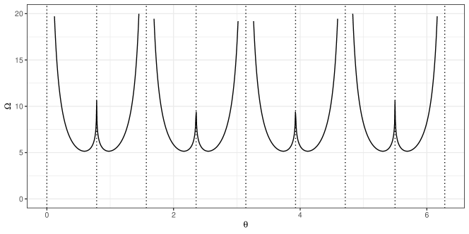
Figure 2: The value of the diffusion coefficient $\Omega=\Omega(\theta)$ for $\theta\in[0,2\pi)$ for the Zig-Zag sampler. The function takes $+\infty$ when $\theta=n\pi/4,n=0,1,\ldots,7$ corresponding to the dotted lines.

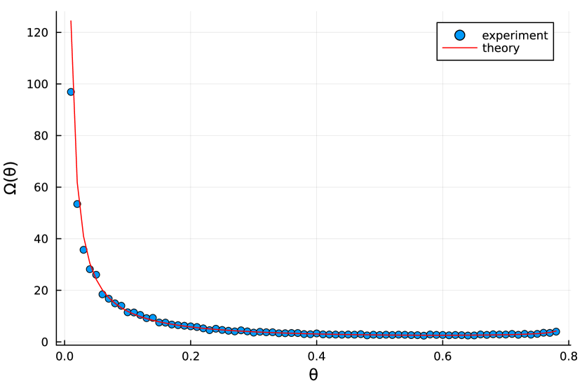
(a) $\theta\in(0,\pi/4)$

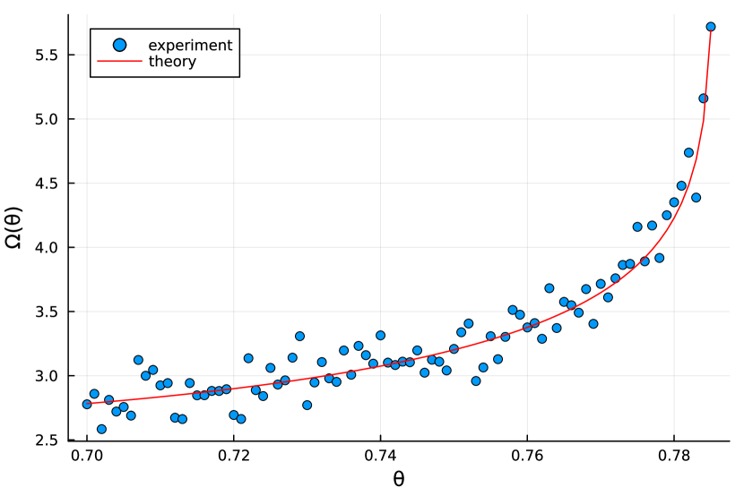
(b) Zoomed in at a sub-interval.

Figure 3: Numerical validation of the theoretical value $\Omega=\Omega(\theta)$ in the range $\theta\in(0,\pi/4)$. This is achieved by statistical estimation of the diffusion coefficient for a grid of values for $\theta$, interpreting the process $y_{1}^{\epsilon}(t)$ as a diffusion. This is for $\epsilon=0.001$ and a trajectory with time horizon $T=2.0$.

2.1.1 The fully and diagonally aligned cases of the Zig-Zag sampler

In this section, we will examine the special cases excluded in Assumption 2.1. When $\theta$ is $\theta=n\pi/4\ (n=0,\ldots,7)$, then $\Omega$ diverges. These eight cases can be further divided into two categories. When $\theta=n\pi/4$ and $n$ is even, either $\cos\theta$ or $\sin\theta=0$ and as a result, $y_{1}$ and $y_{2}$ are independent. The path of $y_{1}$ in this scenario corresponds to the one-dimensional Zig-Zag sampler and exhibits good mixing behaviour without diffusive behaviour. We refer to these cases as the ‘fully aligned’ scenario.

On the other hand, if $\theta$ equals $n\pi/4$ and $n$ is an odd number, the process remains diffusive but now allows for large jumps. These cases are referred to as the ‘diagonally aligned’ scenario. We give an informal but explicit description of how the trajectories behave in this case, and how this differs in comparison to the other cases.

We will make use of the following simple result.

Lemma 2.3.

Suppose $X$ is a positive random variable with hazard rate $(a+\gamma t)_{+}$ for some real number $a$ and positive constant $\gamma$, i.e.,

$$\mathbb{P}(X\geq t)=\exp\left(-\int_{0}^{t}(a+\gamma s)_{+}\,\mathrm{d}s\right),\quad t\geq 0.$$

Then for any positive constant $c$,

$${\mathbb{P}}(X+a\gamma^{-1}\geq c\gamma^{-1/2})=\begin{cases}\exp\left(-c^{2}/2+a_{+}^{2}/2\gamma\right),\quad&c\geq a\gamma^{-1/2},\\ 1,\quad&0\leq c<a\gamma^{-1/2},\end{cases}$$

and

$${\mathbb{E}}(X+a\gamma^{-1})=a_{+}/\gamma+\gamma^{-1/2}\sqrt{2\pi}~{}\Phi(-a_{+}\gamma^{-1})~{}e^{a_{+}^{2}/2\gamma}.$$

By (2.3), we have for a starting position $(y_{1}(0),y_{2}(0),v_{1},v_{2})$ that

$$y_{1}(t)=y_{1}(0)+(v_{1}\cos\theta-v_{2}\sin\theta)t,\quad y_{2}(t)=y_{2}(0)+\varepsilon^{-1}(v_{1}\sin\theta+v_{2}\cos\theta)t$$

until next jump. By the expression from the jump rates in (2.3) the jump rates of the first coordinate and the second coordinate are summarised as

$$\lambda_{1}(t)=(c_{1}+\epsilon^{-1}a_{1}+(1-\gamma_{1})t+\epsilon^{-2}\gamma_{1}t)_{+},\quad\lambda_{2}(t)=(c_{2}+\epsilon^{-1}a_{2}+(1-\gamma_{2})t+\epsilon^{-2}\gamma_{2}t)_{+},\$$

where

$$\gamma_{1}=\sin\theta^{2}+v_{1}v_{2}\sin\theta\cos\theta,\quad\gamma_{2}=\cos\theta^{2}+v_{1}v_{2}\sin\theta\cos\theta$$

and

$$a_{1}=y_{2}v_{1}\sin\theta,\quad a_{2}=y_{2}v_{2}\cos\theta,$$

and $c_{1},c_{2}\in\mathbb{R}$ are constants depending on the initial positions. Note that, if $v_{1}\sin\theta\neq-v_{2}\cos\theta$, then

$$\gamma_{1}+\gamma_{2}=(v_{1}\sin\theta+v_{2}\cos\theta)^{2}>0\quad\Longrightarrow\quad\gamma_{1}>0\ \mathrm{or}\ \gamma_{2}>0.$$

On the other hand, $v_{1}\sin\theta=-v_{2}\cos\theta$ implies that $\gamma_{1}=\gamma_{2}=0$ and one of $a_{1}$ and $a_{2}$ is positive unless $y_{2}=0$. Note that, $|v_{1}\sin\theta|=|v_{2}\cos\theta|$ is satisfied if and only if $\theta$ is in the diagonally aligned cases. Moreover, in this case, the two events $v_{1}\sin\theta=-v_{2}\cos\theta$ and $v_{1}\sin\theta\neq-v_{2}\cos\theta$ occur one after the other and the events are interchanged by jumps.

So by Lemma 2.3, we identify two cases for $(v_{1},v_{2})$:

1. If $v_{1}\sin\theta\neq-v_{2}\cos\theta$ then the next jump time is an $O_{P}(\epsilon)$ random variable;

2. If $v_{1}\sin\theta=-v_{2}\cos\theta$ then the next jump time is an $O_{P}(\epsilon~{}|y_{2}|^{-1})$ random variable.

In fact it is easy to see that from starting values $(y_{1}(0),y_{2}(0))$ on $\mathbb{R}\times\mathbb{R}$ and with any initial velocities, the switch random variables corresponding to $v_{1}$ and $v_{2}$ have explicit hazard rates, many of them in the form of that described in Lemma 2.3 with differing $\gamma$ values summarised in the following result

Proposition 2.4.

With the notation introduced above,

• The next jump distribution is stochastically bounded above by a random variable of the type appearing in Lemma 2.3 with

  $$\gamma=\epsilon^{-2}\max\{\gamma_{1},\gamma_{2}\}$$

  with $a=\max\{c_{1},c_{2}\}+\epsilon^{-1}\max\{a_{1},a_{2}\}$.

• If $\theta\neq(2n+1)\pi/4$, then uniformly over the state space, as $\epsilon\to 0$ and the next jump distribution is bounded above by a $O_{P}(\epsilon)$ random variable.

• If $\theta=(2n+1)\pi/4$, then two subsequent jump distributions are of the order of $O(\epsilon~{}|y_{2}|^{-1})$ and $O_{P}(\epsilon)$ in turn.

Thanks to these observations, and also by the simulation results, we conjecture that the process $y_{1}$ converges to a diffusion with jumps in this case. Here, the jump occurs when $|y_{2}|$ is small. However, this case is technically challenging. In a real-world application the narrow posterior distribution will likely not be perfectly aligned with the diagonal, and in an exceptional case of perfect diagonal alignment we expect a better performance compared to our worst case analysis for the non-aligned case.

2.2 The Bouncy Particle Sampler in the two dimensional case

Next, we present the asymptotic behaviour for the Bouncy Particle Sampler (BPS) for $d=2$. The BPS is rotationally invariant and we may therefore assume $U=I_{d}$ without loss of generality. The associated generator in terms of the coordinates $(x,v)$ is given by equation (3.2). With the reparametrisation in (2.2), the generator can be expressed as

$$\mathcal{L}^{\epsilon}f(y,v) =v_{1}\partial_{y_{1}}f(y,v)+\epsilon^{-1}v_{2}\partial_{y_{2}}f(y,v)+(v_{1}y_{1}+\epsilon^{-1}v_{2}y_{2})_{+}~{}(\mathcal{B}^{\epsilon}-\operatorname{{id}})f(y,v),$$

where we omit the refreshment term for simplicity (see Remark 2.1 below), and where the operator $\mathcal{B}^{\epsilon}$ is given as the pullback of the reflection

$$(y,v)\quad\mapsto\quad\left(y,\quad v-2\frac{v_{1}y_{1}+\epsilon^{-1}v_{2}y_{2}}{y_{1}^{2}+\epsilon^{-2}y_{2}^{2}}\begin{pmatrix}y_{1}\\ \epsilon^{-1}y_{2}\end{pmatrix}\right)=:\left(y,v+\begin{pmatrix}\Delta^{\epsilon}v_{1}\\ \Delta^{\epsilon}v_{2}\end{pmatrix}\right).$$

Observe that the jump size $\Delta^{\epsilon}v_{1}$ of $v_{1}$ induced by $\mathcal{B}^{\epsilon}$ satisfies

$$\epsilon^{-1}\Delta^{\epsilon}v_{1}\longrightarrow_{\epsilon\rightarrow 0}\quad-2\frac{v_{2}~{}y_{2}}{y_{2}^{2}}~{}y_{1}.$$ (2.6)

Our first observation is that, as shown in Figure 5, the process of $\mathrm{sgn}(v_{2})$ and that of $y_{2}$ mixes well but that of $(y_{1},v_{1})$ does not. This is not surprising given the form of the generator. When $\epsilon$ is small enough, the process of $(y_{2},v_{2})$ is asymptotically dominated by the generator $\mathcal{L}_{0}$ corresponding to the one-dimensional Zig-Zag sampler

$$\mathcal{L}_{0}f(y,v) =v_{2}\partial_{y_{2}}f(y,v)+(v_{2}y_{2})_{+}~{}(\mathcal{B}^{0}-\operatorname{{id}})f(y,v)$$

where $\mathcal{B}^{0}$ is given as the pullback of the coordinate reflection

$$(x,v)\mapsto\left(x,\begin{pmatrix}v_{1}\\ -v_{2}\end{pmatrix}\right)$$

Note that the value of $|v_{2}|$ remains unchanged by the dynamics generated by $\mathcal{L}_{0}$.

The second observation is that, as in Figure 4, the process $(y_{1},v_{1})$ (and $|v_{2}|$) mixes slowly and vaguely follows a periodic orbit. The process of $y_{1}$ satisfies $\frac{\mathrm{d}}{\mathrm{d}t}y_{1}=v_{1}$. Although the process of $v_{1}$ is driven by the reflection jump, the jump size becomes so small that it asymptotically follows

$$\frac{\mathrm{d}}{\mathrm{d}t}v_{1}=(v_{2}y_{2})_{+}~{}\left(-2\frac{v_{2}y_{2}}{y_{2}^{2}}y_{1}\right)=-2v_{2}^{2}~{}1_{\{v_{2}y_{2}>0\}}y_{1}$$

as $\epsilon\rightarrow 0$ by (2.6). Observe that the value of $|v|=\sqrt{v_{1}^{2}+v_{2}^{2}}$ does not change during the dynamics. Thus, for $\kappa^{2}:=|v(0)|^{2}$, we have $|v_{2}|=\sqrt{\kappa^{2}-v_{1}^{2}}$. Also, the fast mixing component $(y_{2},\mathrm{sgn}(v_{2}))$ is averaged out by $\mathcal{N}(0,1)\otimes\mathcal{U}(\{-1,+1\})$, and we obtain the dynamics

$$\frac{\mathrm{d}}{\mathrm{d}t}\begin{pmatrix}y_{1}\\ v_{1}\end{pmatrix}=\begin{pmatrix}v_{1}\\ -(\kappa^{2}-v_{1}^{2})y_{1}\end{pmatrix}.$$ (2.7)

See the red lines of Figure 4.

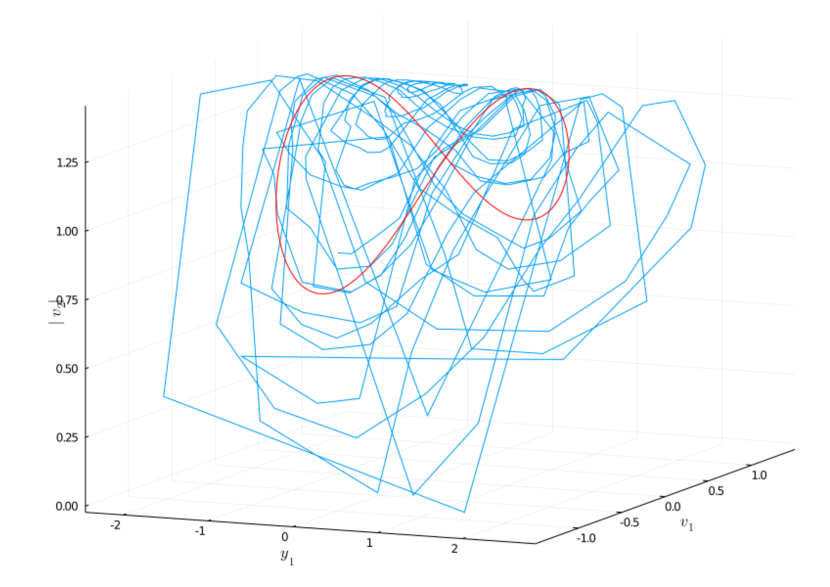
(a) $\epsilon=0.1$

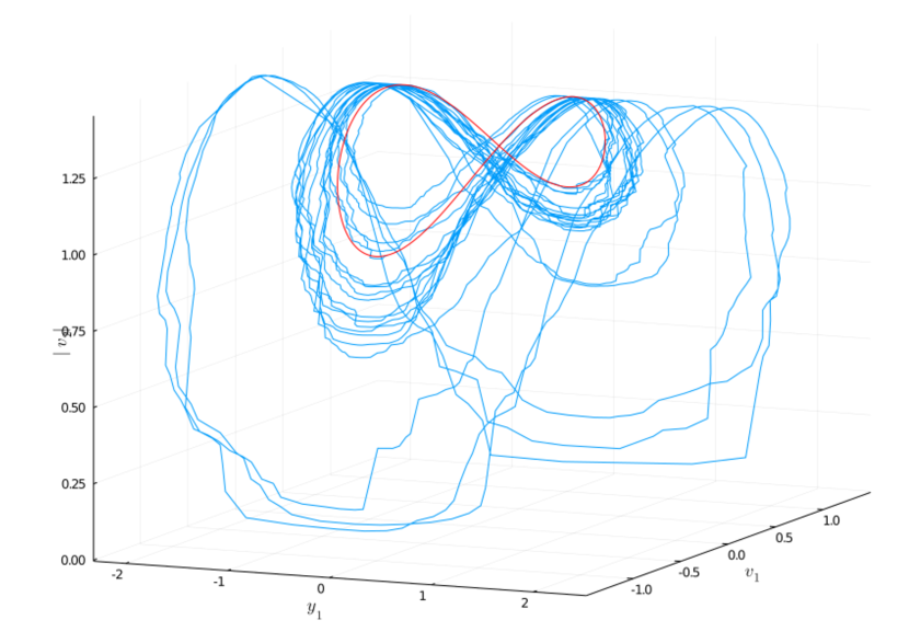
(b) $\epsilon=0.01$

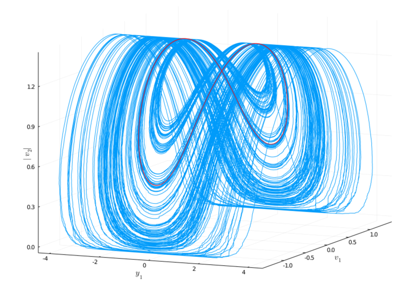
(c) $\epsilon=10^{-4}$

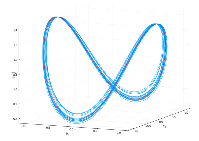
(d) $\epsilon=10^{-5}$

Figure 4: Numerical experiment illustrating how the $(y_{1}(t),v_{1}(t),|v_{2}|(t))$ statistics of a BPS trajectory (in blue) converge to the fluid limit (in red) given by (2.7).

This dynamics preserves the value of $y_{1}^{2}+\log(|v(0)|^{2}-v_{1}^{2})$. Let $(y_{1}^{\epsilon}(t),v_{1}^{\epsilon}(t))$ be the $(y_{1},v_{1})$-coordinate of the bouncy particle sampler process. We have the following convergence result.

Theorem 2.5.

The stationary process $(y_{1}^{\epsilon}(t),v_{1}^{\epsilon}(t))$ converges to the solution of the differential equation (2.7) in the sense that

$$\sup_{0\leq t\leq T}|y_{1}^{\epsilon}(t)-y_{1}(t)|+|v_{1}^{\epsilon}(t)-v_{1}(t)|\longrightarrow_{\epsilon\rightarrow 0}0$$

in probability for any $T>0$ where $(y_{1}^{\epsilon}(0),v_{1}^{\epsilon}(0))=(y_{1}(0),v_{1}(0))$, $\kappa^{2}=|v^{\epsilon}(0)|^{2}$.

Proof.

The claim follows from the general result Theorem 3.4replacing $c(\alpha,\beta)$ by $\mathbb{E}[(v_{2}y_{2})_{+}^{2}/|y_{2}|^{2}]=1/2$ since the Skorokhod topology is equivalent to the local uniform topology when the limit process is continuous as described in page 124 of Section 12 of [8]. ∎

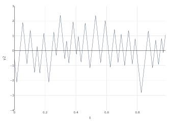
Figure 5: Paths of $v_{2}$ (left) and $y_{2}$ (right) for the Bouncy particle sampler for $\epsilon=0.01$.

Remark 2.1.

For simplicity we have assumed the refreshment to be equal to zero. The only thing that would change for a fixed refreshment rate would be that the process $(y_{1},y_{2},v_{1},v_{2})$ would experience refreshments at $O_{P}(1)$ random times. The trajectory between refreshments would not be affected by these refreshments, aside from having a new initial velocity vector. For the multi-dimensional case with refreshment jumps, refer to Theorem 3.4

2.3 Discussion of the two-dimensional case

Both the Zig-Zag Sampler (ZZS) and the Bouncy Particle Sampler (BPS) are capable of simulating anisotropic target distribution. However, the asymptotic behaviour of the two methods is systematically different. The former converges to a diffusion process and the latter to a deterministic periodic orbit. Moreover, the number of jumps to convergence is $O(\epsilon^{-2})$ for the ZZS (except for the non-generic, aligned cases), and $O(\epsilon^{-1})$ for the BPS. Therefore, the BPS is efficient in this scenario, which is in stark contrast to the high-dimensional, factorised scenario studied in [6].

The behaviour of the Zig-Zag sampler is divided into three categories: Fully aligned, diagonally-aligned, and non-aligned. We are not yet fully able to understand the asymptotic behaviour of the diagonally aligned case. However, we conjecture that it converges to a diffusion with jumps.

For a discussion on a multi-dimensional scenario and a comparison of the computational complexity between PDMPs and the random walk Metropolis algorithm, please refer to Section 6.

Method	$\sharp$ Events/unit time	Time until convergence	Combined effort
ZZ ($\theta\neq n\pi/4$)	$O(\epsilon^{-1})$	$O(\epsilon^{-1})$	$O(\epsilon^{-2})$
ZZ ($\theta=n\pi/4$)	$O(\epsilon^{-1})$	$O(1)$	$O(\epsilon^{-1})$
BPS	$O(\epsilon^{-1})$	$O(1)$	$O(\epsilon^{-1})$

Table 1: Computational effort of the piecewise deterministic processes.

3 Main results and proof strategy

Let $d\geq 2$ be an integer, and let $\mathrm{K}$ and $\mathrm{L}$ be a partition of $\{1,\ldots,d\}$ that is,

$$\mathrm{K}\cup\mathrm{L}=\{1,\ldots,d\},\quad\mathrm{K}\cap\mathrm{L}=\emptyset$$

and $0<\sharp\mathrm{K}=k$ and $0<\sharp\mathrm{L}=l=d-k$. The target probability distribution is $\mathcal{N}_{d}(0,\Sigma^{\epsilon})$ where the $d\times d$-symmetric positive definite matrix $\Sigma^{\epsilon}$ has the eigen decomposition

$$\Sigma^{\epsilon}=U^{\top}(\Lambda^{\epsilon})^{2}U,\ \Lambda^{\epsilon}=\operatorname{diag}(\Lambda_{\mathrm{K}},\epsilon~{}\Lambda_{\mathrm{L}})$$

where $\Lambda_{\mathrm{K}}$ and $\Lambda_{\mathrm{L}}$ are $k\times k$ and $l\times l$ diagonal matrices with strictly positive diagonal elements, and $U$ is an orthogonal matrix with decomposition

$$U=\begin{pmatrix}U_{\mathrm{K}}&U_{\mathrm{K}\mathrm{L}}\\ U_{\mathrm{K}\mathrm{L}}^{\top}&U_{\mathrm{L}}\end{pmatrix}.$$

In this paper, we will study two kinds of extended generators, the Zig-Zag sampler defined on $\mathbb{R}^{d}\times\{-1,+1\}^{d}$ and the bouncy particle sampler defined on $\mathbb{R}^{d}\times\mathbb{R}^{d}$:

$$\text{ZZS}:\quad\mathfrak{L}^{\epsilon}f(x,v) =\sum_{i=1}^{d}v_{i}\partial_{x_{i}}f(x,v)+\sum_{i=1}^{d}(v_{i}((\Sigma^{\epsilon})^{-1}x)_{i})_{+}(f(x,F_{i}(v))-f(x,v))$$ (3.1)

$$\text{BPS}:\quad\mathfrak{L}^{\epsilon}f(x,v) =v^{\top}\partial_{x}f(x,v)+(v^{\top}(\Sigma^{\epsilon})^{-1}x)_{+}~{}(\mathfrak{B}^{\epsilon}-\operatorname{{id}})+\rho~{}\left(\mathcal{R}-\operatorname{id}\right)$$ (3.2)

where the switch function $F_{i}(v)$ switches the sign of the $i$-th coordinate of $v$, and the reflection operator $\mathfrak{B}^{\epsilon}$ is a deterministic operation such that

$$(x,v)\quad\mapsto\quad\left(x,\quad v-2v^{\top}(\Sigma^{\epsilon})^{-1}x~{}\frac{(\Sigma^{\epsilon})^{-1}x}{|(\Sigma^{\epsilon})^{-1}x|^{2}}\right).$$

The constant $\rho\geq 0$ is called the refreshment rate, and the refresh operator $\mathcal{R}$ is defined by

$$(\mathcal{R}f)(x,v)=\int_{\mathbb{R}^{d}}f(x,w)\phi(w)\mathrm{d}w$$

where $\phi(w)$ is the probability density function of the $d$-dimensional standard normal distribution. The domains of the extended generators are the set of bounded functions on $(x,v)\in\mathbb{R}^{d}\times\{-1,+1\}^{d}$ and $(x,v)\in\mathbb{R}^{d}\times\mathbb{R}^{d}$ such that each function is differentiable in $x$. The cores of the extended generators have also been studied such as [12, 16].

3.1 Main results for the Zig-Zag sampler

With the reparametrisation (2.2), the extended generator of the Zig-Zag process $\xi^{\epsilon}(t)=(y^{\epsilon}(t),v^{\epsilon}(t))$ is

$$\mathcal{L}^{\epsilon}f(y,v)=((\Lambda^{\epsilon})^{-1}Uv)^{\top}\partial_{y}f(y,v)+\sum_{i=1}^{d}(v_{i}(U^{\top}(\Lambda^{\epsilon})^{-1}y)_{i})_{+}~{}(\mathcal{F}_{i}-\operatorname{id})f(y,v).$$ (3.3)

We decompose the $d$-dimensional vector $y$ into $\mathrm{K}$ and $\mathrm{L}$ components, i.e., $y=(y_{\mathrm{K}},y_{\mathrm{L}})$. When $\epsilon$ is small, except for some special cases, the process of $(y_{\mathrm{L}},v)$ mixes well but that of $y_{\mathrm{K}}$ does not. We are interested in the latter behaviour since the slowest dynamics reflects the total computational cost of Monte Carlo methods. The limit process of the faster dynamics $(y_{\mathrm{L}},v)$ is characterised by the extended generator

$$\mathcal{L}_{0}=(\Lambda_{\mathrm{L}}^{-1}(Uv)_{\mathrm{L}})^{\top}\partial_{y_{\mathrm{L}}}+\sum_{i=1}^{d}(v_{i}(U_{{}_{\mathrm{L}},\cdot}^{\top}\Lambda_{\mathrm{L}}^{-1}y_{\mathrm{L}})_{i})_{+}~{}(\mathcal{F}_{i}-\operatorname{id}).$$ (3.4)

Before discussing the asymptotic result, we describe the special cases mentioned above. In the two-dimensional case described in Section 2.1, $\theta=n\pi/4\ (n=0,\ldots,7)$ were excluded in the analysis, which corresponds to the case where the Markov process with generator $\mathcal{L}_{0}$ is not ergodic as a process of $(y_{2},v)$. Ergodicity is related to the $d\times d$-positive semidefinite matrix

$$\Sigma_{\mathrm{L}}=U_{\mathrm{L},\cdot}^{\top}\Lambda_{\mathrm{L}}^{-2}U_{\mathrm{L},\cdot}.$$

If $v_{i}(\Sigma_{\mathrm{L}}v)_{i}>0$, then the $i$-th component $v_{i}$ is flippable with direction $v$, in the sense that if the process maintains direction $v$, there is a positive probability of switching the sign of the $i$-th component of $v$ when $t$ is large enough. Indeed,

$$(v_{i}(t)(U_{{}_{\mathrm{L}},\cdot}^{\top}\Lambda_{\mathrm{L}}^{-1}y_{\mathrm{L}}(t))_{i})=(v_{i}(U_{{}_{\mathrm{L}},\cdot}^{\top}\Lambda_{\mathrm{L}}^{-1}y_{\mathrm{L}}(0))_{i}+t~{}v_{i}(\Sigma_{\mathrm{L}}v)_{i})>0$$

when $t$ is large enough, where $v(t)=(v_{1}(t),\ldots,v_{d}(t))=v$, and $y_{\mathrm{L}}(t)=y_{\mathrm{L}}(0)+t~{}\Lambda_{\mathrm{L}}^{-1}(Uv)_{\mathrm{L}}$. We assume the following condition for flippability, which ensures the ergodicity of the process.

Assumption 3.1.

$v^{\top}\Sigma_{\mathrm{L}}v>0$ for any $v\in\{-1,0,+1\}^{d}\backslash\mathbf{0}$.

As described above, the process $(y^{\epsilon}_{\mathrm{L}}(t),v^{\epsilon}(t))$ converges weakly to a Markov process with an extended generator $\mathcal{L}_{0}$. However, in the same time scale, the process $y_{\mathrm{K}}^{\epsilon}(t)$ becomes degenerate. To address this, we must scale time appropriately. Specifically, we require $O(\epsilon^{-1})$ time for mixing. The proof will be presented at the end of Section 4.2.

Theorem 3.2.

As $\epsilon\rightarrow 0$, under Assumption 3.1, and if $\xi^{\epsilon}(0)$ follows the stationary distribution $\mathcal{N}(0,I_{d})\otimes\mathcal{U}(\{-1,+1\}^{d})$, then $y_{\mathrm{K}}^{\epsilon}(\epsilon^{-1}t)$ converges to an Ornstein–Uhlenbeck process defined in (4.4) in the Skorokhod topology.

Under the same conditions as in Theorem 3.2, we examine the quantity $N_{T}^{\epsilon}$ which represents the number of jumps in the process $(y^{\epsilon}(t),v^{\epsilon}(t))$ over the time interval of $[0,T]$. The number of jumps, $N_{T}^{\epsilon}$, is an indicator of the computational cost per unit time. Let $\Sigma^{\epsilon}_{i,i}$ and $(\Sigma_{\mathrm{L}})_{i,i}$ represent the $i$-th diagonal entries of the matrices $\Sigma^{\epsilon}$ and $\Sigma_{\mathrm{L}}$, respectively. The proof is postponed to Section 4.3.

Based on the following theorem, we can conclude that $\mathbb{E}[N_{T}^{\epsilon}]=O(\epsilon^{-1}T)$. This implies that $O(\epsilon^{-2})$ jumps are required to achieve mixing, as we make precise in the following result.

Theorem 3.3.

Under the same conditions as Theorem 3.2, the expected number of jumps of $(y^{\epsilon}(t),v^{\epsilon}(t))$ in the time interval $[0,T]$ is

$$\mathbb{E}[N_{T}^{\epsilon}]=\frac{T}{2\sqrt{2\pi}}\sum_{i=1}^{d}\sqrt{\Sigma^{\epsilon}_{i,i}}.$$

In particular,

$$\lim_{\epsilon\rightarrow 0}\epsilon~{}\mathbb{E}[N_{T}^{\epsilon}]=\frac{T}{2\sqrt{2\pi}}\sum_{i=1}^{d}\sqrt{(\Sigma_{\mathrm{L}})_{i,i}}.$$

3.2 Main results for the Bouncy Particle Sampler

With the reparametrisation (2.2), the extended generator of the Bouncy particle sampler process $\xi^{\epsilon}(t)=(y^{\epsilon}(t),v^{\epsilon}(t))$ is

$$\mathcal{L}^{\epsilon}=((\Lambda^{\epsilon})^{-1}v)^{\top}\partial_{y}+(v^{\top}(\Lambda^{\epsilon})^{-1}y)_{+}~{}(\mathcal{B}^{\epsilon}-\operatorname{{id}})+\rho~{}\left(\mathcal{R}-\operatorname{id}\right)$$ (3.5)

where the reflection operator is defined by $\mathcal{B}^{\epsilon}f(y,v)=f(y,B^{\epsilon}(y)v)$ and

$$B^{\epsilon}(y)v=v-2v^{\top}(\Lambda^{\epsilon})^{-1}y~{}\frac{(\Lambda^{\epsilon})^{-1}y}{|(\Lambda^{\epsilon})^{-1}y|^{2}}.$$ (3.6)

The refreshment rate $\rho$ is a positive constant, and the refreshment operator is defined by

$$\mathcal{R}f(x,v)=\int_{\mathbb{R}^{d}}f(x,u)\phi(u)\mathrm{d}u.$$

Unlike Zig-Zag sampler case, without loss of generality, we can assume $\Sigma^{\epsilon}=(\Lambda^{\epsilon})^{2}$ since the process is rotationally invariant. Let $y^{\epsilon}(t)=(y^{\epsilon}_{\mathrm{K}}(t),y^{\epsilon}_{\mathrm{L}}(t))$ and $v^{\epsilon}(t)=(v^{\epsilon}_{\mathrm{K}}(t),v^{\epsilon}_{\mathrm{L}}(t))$. In two dimensional case in Section 2.2, $(y_{2},v_{2})$ mixes faster and $(y_{1},v_{1})$ mixes slower. Similarly, in the general case, $(y_{\mathrm{L}},v_{\mathrm{L}})$ mixes faster except some statistics described below, and $(y_{\mathrm{K}},v_{\mathrm{K}})$ mixes slower.

The limit behaviour depends on the value of $\Lambda_{\mathrm{L}}$. For the sake of simplicity, we assume $\Lambda_{\mathrm{L}}$ is the identity matrix. In this case, $\alpha=|v_{\mathrm{L}}|^{2}$, and $\beta=|v_{\mathrm{L}}|^{2}|y_{\mathrm{L}}|^{2}-(v_{\mathrm{L}}^{\top}y_{\mathrm{L}})^{2}$ are fixed constants, and $(y_{\mathrm{L}},v_{\mathrm{L}})$ is always on a two dimensional hyperplane. This hyperplane will be refreshed at the refreshment jump time. In the asymptotic analysis, we need to study not only $(y_{\mathrm{K}},v_{\mathrm{K}})$ but also $(\alpha,\beta)$ together with the effect of refreshment. The limit process is a little complicated, and so we will describe it later in Section 5.2.3. The proof of the following theorem is also in the section. Let $(\alpha^{\epsilon}(t),\beta^{\epsilon}(t))$ be the corresponding process of the statistics $(\alpha,\beta)$.

Theorem 3.4.

As $\epsilon\rightarrow 0$, if $\Lambda_{\mathrm{L}}=I_{\mathrm{L}}$ and if $\xi^{\epsilon}(0)$ follows the stationary distribution $\mathcal{N}(0,I_{d})\otimes\mathcal{N}(0,I_{d})$, the Markov process $(y^{\epsilon}_{\mathrm{K}}(t),v^{\epsilon}_{\mathrm{K}}(t),\alpha^{\epsilon}(t),\beta^{\epsilon}(t))$ converges to an ordinary differential equation with jumps which will be defined in (5.25) in the Skorokhod topology.

Let $N_{T}^{\epsilon}$ be the number of jumps of the process $(y^{\epsilon}(t),v^{\epsilon}(t))$ within the time interval of $[0,T]$. Based on the following theorem, we can conclude that $\mathbb{E}[N_{T}^{\epsilon}]=O(\epsilon^{-1}T)$. This implies that $O(\epsilon^{-1})$ jumps are required to achieve mixing. The proof of the following theorem is postponed until Section 5.3.

Theorem 3.5.

Under the same conditions as those for Theorem 3.4, the expected number of jumps of $(y^{\epsilon}(t),v^{\epsilon}(t))$ in the time interval $[0,T]$ is

$$\mathbb{E}[N_{T}^{\epsilon}]\leq\frac{T}{2}(\mathrm{diag}((\Lambda^{\epsilon})^{-1})+2\rho).$$

Also,

$$\lim_{\epsilon\rightarrow 0}\epsilon~{}\mathbb{E}[N_{T}^{\epsilon}]=\frac{T}{2\sqrt{\pi}}~{}\frac{\Gamma((l+1)/2)}{\Gamma(l/2)}.$$

3.3 Proof strategy

We shall require multi-scale analysis in the proofs of our main results, and will therefore rely heavily on the homogenisation and averaging techniques of [22]. We define $u(x,v,t)=\mathbb{E}[\phi(\xi^{\epsilon}(t))|\xi^{\epsilon}(0)=(x,v)]$ for a real-valued function $\phi$. Under certain regularity conditions, the function $u$ satisfies the backward Kolmogorov equation which can be expressed as

$$\frac{\mathrm{d}u}{\mathrm{d}t}=\mathcal{L}^{\epsilon}u$$

where $\mathcal{L}^{\epsilon}$ is the extended generator. The scaling limit of the extended generator $\mathcal{L}^{\epsilon}$ can be analysed by using the expansion of this differential equation in powers of a small parameter $\epsilon$.

To understand the scaling limit of the Zig-Zag sampler, we employ the homogenisation approach. Specifically, we solve the differential equation

$$\epsilon~{}\frac{\mathrm{d}u}{\mathrm{d}t}=\mathcal{L}^{\epsilon}u.$$ (3.7)

where the factor $\epsilon$ on the left-hand side represents time scaling. The extended generator $\mathcal{L}^{\epsilon}$ is then expanded into $\mathcal{L}^{\epsilon}=\epsilon^{-1}\mathcal{L}_{0}+\mathcal{L}_{1}+o(1)$ and the function $u$ is expanded into

$$u=u_{0}+\epsilon u_{1}+\epsilon^{2}u_{2}+o(\epsilon^{2}).$$

This leads to a system of equations

$$\begin{cases}0&=\mathcal{L}_{0}u_{0}\\ 0&=\mathcal{L}_{0}u_{1}+\mathcal{L}_{1}u_{0}\\ \frac{\mathrm{d}u_{0}}{\mathrm{d}t}&=\mathcal{L}_{0}u_{2}+\mathcal{L}_{1}u_{1}\end{cases}$$ (3.8)

at orders $O(\epsilon^{-1}),O(1)$ and $O(\epsilon)$ of the backward Kolmogorov equation. The system can be used to derive a second-order differential equation for a function $u_{0}$, given by

$$\frac{\mathrm{d}u_{0}}{\mathrm{d}t}=f(u_{0}),$$

which characterise the limit of the process $\xi^{\epsilon}(t)$. The expression of $f$ will be described later.

The bouncy particle sampler can be analysed using the averaging approach of [22]. This technique involves a different expansion of the Kolmogorov backward equation leading to a set of equations given by

$$\begin{cases}0&=\mathcal{L}_{0}u_{0}\\ \frac{\mathrm{d}u_{0}}{\mathrm{d}t}&=\mathcal{L}_{0}u_{1}+\mathcal{L}_{1}u_{0}.\end{cases}$$

Solving this set of equations leads to a first-order differential equation that characterises the scaling limit of the bouncy particle sampler.

4 Convergence of the Zig-Zag sampler

4.1 Properties of the leading-order generator

The reparametrised extended generator of the Zig-Zag sampler (2.2) has a formal expansion

$$\mathcal{L}^{\epsilon}=\epsilon^{-1}\mathcal{L}_{0}+\mathcal{L}_{1}+o(\epsilon)$$

where

$$\begin{split}\mathcal{L}_{0}&=(\Lambda_{\mathrm{L}}^{-1}(Uv)_{\mathrm{L}})^{\top}\partial_{y_{\mathrm{L}}}+\sum_{i=1}^{d}(v_{i}(U_{{}_{\mathrm{L}},\cdot}^{\top}\Lambda_{\mathrm{L}}^{-1}y_{\mathrm{L}})_{i})_{+}~{}(\mathcal{F}_{i}-\operatorname{id})\\ \mathcal{L}_{1}&=(\Lambda_{\mathrm{K}}^{-1}(Uv)_{\mathrm{K}})^{\top}\partial_{y_{\mathrm{K}}}+\sum_{i=1}^{d}(v_{i}(U_{\mathrm{K},\cdot}^{\top}\Lambda_{\mathrm{K}}^{-1}y_{\mathrm{K}})_{i})~{}1(v_{i}(U_{{}_{\mathrm{L}},\cdot}^{\top}\Lambda_{\mathrm{L}}^{-1}y_{\mathrm{L}})_{i}\geq 0)~{}(\mathcal{F}_{i}-\operatorname{id}).\end{split}$$ (4.1)

We consider the operator $\mathcal{L}_{0}$ as an operator of $(y_{\mathrm{L}},v)$-valued functions, where $y_{\mathrm{K}}$ is fixed. We establish the ergodicity of $\mathcal{L}_{0}$ by following the methodology outlined in [7]. However, we need to make some modifications to the arguments in [7] since the velocity in $\mathcal{L}_{0}$ is not aligned with the coordinates.

If $E$ is a topological space, a Markov process is called a $T$-process if there exists a probability measure $a$ on $[0,\infty)$, a lower semicontinuous, non-trivial semi Markov kernel $T$ such that $P_{a}(x,A)\geq T(x,A)\ (x\in E,A\in\mathcal{E})$ where $P_{a}(x,A)=\int P_{t}(x,A)a(\mathrm{d}t)$. Let

$$\mu=\mathcal{N}_{\mathrm{L}}(0,I_{\mathrm{L}})\otimes\mathcal{U}(\{-1,+1\}^{d}).$$

Lemma 4.1.

Under Assumption 3.1, the Markov process corresponding to the extended generator $\mathcal{L}_{0}$ is a $T$-process, ergodic and the invariant measure is $\mu$.

Proof.

The core of the generator is $C_{c}^{\infty}(\mathbb{R}^{l}\times\mathbb{R}^{d})$ as proven in Corollary 6.2 of [16]. Consequently, $\mu$ is the invariant measure of the semigroup by Proposition 4.9.2 of [13]. The rest of the proof is essentially the same as that of Section 2.2 and Section 3 of [7]. Section 2.2 shows that for a multivariate normal target distribution, any state $z$ is reachable from any other state $z^{\prime}$ in the sense that there is a piecewise deterministic path of $\mathcal{L}_{0}$ from $z^{\prime}$ to $z$ such that the corresponding jump intensity is strictly positive at each jump point. In our case, $e_{1},\ldots,e_{d}$ in Corollary 2 of the paper are replaced by $\Lambda_{\mathrm{L}}^{-1}(Ue_{i})_{\mathrm{L}}\ (i=1,\ldots,d)$, where $e_{i}\in\mathbb{R}^{d}$ is a vector which is $1$ at the $i$-th component and all other components are $0$. Therefore, the number of velocity vectors is larger than the dimension of $y_{\mathrm{L}}$, and the velocity vectors are angled. Nonetheless, we show that still, the argument in Section 2.2 is applicable to this case.

We apply Lemmas 1-3 of their paper to this case. By Assumption 3.1, Lemmas 1 and 3 of their paper can be directly applicable and so we focus on Lemma 2. The lemma states that for any $y,y^{\prime}\in\mathbb{R}^{d}$, the state $(y^{\prime},-v)$ is reachable from $(y,v)$. Observe that

$$\Lambda_{\mathrm{L}}^{-1}(Ue_{i})_{\mathrm{L}}=\Lambda_{\mathrm{L}}^{-1}U_{\mathrm{L}}(e_{i})_{\mathrm{L}}\ (i\in\mathrm{L}).$$

By applying a linear transformation $x\mapsto U_{\mathrm{L}}^{-1}\Lambda_{\mathrm{L}}x$, the argument in Lemma 2 [7] can be directly applied to the irreducibility proof of $\mathcal{L}_{0}$ if we omit $\Lambda_{\mathrm{L}}^{-1}(Ue_{i})_{\mathrm{L}}\ (i\in\mathrm{K})$. The proof will be carried out if we can handle the omitted component. On the other hand, thanks to Assumption 3.1, the components in $\mathrm{K}$ are asymptotically flippable in the sense that any coordinate can be switched after some time. Therefore, the argument in Lemma 2 can be applied to the current case after switching all $\mathrm{K}$ components. From this, the assertion follows. ∎

We prove exponential ergodicity of $\mathcal{L}_{0}$ by showing exponential drift inequality. A slight modification of the drift function in Lemma 11 of [7] can be applied in this case. In the following, we apply the linear operators $\mathcal{L}_{0}$ and $\mathcal{L}_{1}$ to vector valued functions coordinatewise.

Proposition 4.2.

The extended generator $\mathcal{L}_{0}$ is exponentially ergodic as an operator of the variable $(y_{\mathrm{L}},v)$. In particular, there is a solution $\chi_{0}:\mathbb{R}^{l}\times\mathbb{R}^{d}\rightarrow\mathbb{R}^{d}$ of the Poisson equation $\mathcal{L}_{0}\chi_{0}(y_{\mathrm{L}},v)=v$, and it is unique up to a constant. Moreover, for any $c>0$ there is a constant $c_{0}$ such that $|\chi_{0}|\leq c_{0}\exp(c|y_{\mathrm{L}}|^{2})$. In particular, $\chi_{0}(y_{\mathrm{L}},v)$ has an arbitrary order of moments.

Proof.

As in Lemma 11 of [7], the exponential drift inequality can be determined by the drift function

$$V(y_{\mathrm{L}},v)=\exp\left(\alpha~{}|y_{\mathrm{L}}|^{2}/2+\sum_{i=1}^{d}\kappa(v_{i}(U_{\mathrm{L},\cdot}^{\top}\Lambda_{\mathrm{L}}^{-1}y_{\mathrm{L}})_{i})\right)$$

where $0<\alpha<1$ and $\kappa(s)=\operatorname{sgn}(s)\log(1+|s|)$. By Theorem 3.2 of [14], since $v$ is bounded, there is a solution to the Poisson equation for $\mathcal{L}_{0}\chi_{0}=v$ and the solution satisfies $|\chi_{0}|\leq c_{0}(V+1)$ for some constant $c_{0}>0$. Thus the first claim follows since $\kappa(s)\leq|s|\leq 1+|s|^{2}$. Also, since we can take $\alpha\leq 1/m$ for any $m\in\mathbb{N}$, the solution has the $m$-th order of moment. ∎

Lemma 4.3.

The solution $\chi_{0}(y_{\mathrm{L}},v)$ of the Poisson equation $\mathcal{L}_{0}\chi_{0}=v$ is in the domain of the extended generator $\mathcal{L}^{\epsilon}$, as a function of $(y,v)$.

Proof.

The solution $\chi_{0}$ is included in the domain of the extended generator $\mathcal{L}_{0}$ by construction. The domain of $\mathcal{L}^{\epsilon}$ is characterised by conditions (i-iii) of Theorem 5.5 of [10]. The map $t\mapsto\chi_{0}(y_{\mathrm{L}}+t~{}\Lambda_{\mathrm{L}}^{-1}(Uv)_{\mathrm{L}},v)$ is absolutely continuous, so the it satisfies condition (i). Moreover, $|\chi_{0}|\leq c_{0}\exp(c|y_{\mathrm{L}}|^{2})$ for constants $c,c_{0}>0$, which means that the local integrability condition for $(\mathcal{F}_{i}-\mathrm{id})\chi_{0}$ in (iii) of Theorem 5.5 is also satisfied for $i=1,\ldots,d$. The generator $\mathcal{L}^{\epsilon}$ is no boundary, so it satisfies condition (ii). By Theorem 5.5, the function $\chi_{0}$ is in the domain of the extended generator $\mathcal{L}^{\epsilon}$. ∎

In the next section, we will show that the process of $y_{\mathrm{K}}$ converges to the Ornstein–Uhlenbeck process. The drift and the diffusion coefficients are expressed by the solution $\chi:\mathbb{R}^{l}\times\mathbb{R}^{d}\rightarrow\mathbb{R}^{k}$ of the Poisson equation

$$\mathcal{L}_{0}\chi(y_{\mathrm{L}},v)=-\mathcal{L}_{1}\psi(y,v)=-(\Lambda_{\mathrm{K}}^{-1}(Uv)_{\mathrm{K}}),$$ (4.2)

for $\psi(y,v)=y_{\mathrm{K}}$ which has an expression

$$\chi(y_{\mathrm{L}},v)=-(\Lambda_{\mathrm{K}}^{-1}(U\chi_{0})_{\mathrm{K}}).$$ (4.3)

Then the limit Ornstein–Uhlenbeck process is expressed as

$$\mathrm{d}X(t)=-\frac{1}{2}\Upsilon~{}X(t)\mathrm{d}t+\Omega^{1/2}~{}\mathrm{d}W(t)$$ (4.4)

where $W(t)$ is the $k$-dimensional standard Wiener process, and $\Omega$ and $\Upsilon$ are $k\times k$ matrices defined by

$$\Omega=-~{}\mu((\mathcal{L}_{0}\chi)~{}\chi^{\top}+\chi~{}(\mathcal{L}_{0}\chi)^{\top}),\quad\Upsilon=-2\mu\left(\chi~{}(\mathcal{L}_{0}\chi)^{\top}\right)~{}\Longrightarrow~{}\Omega=\frac{\Upsilon+\Upsilon^{\top}}{2}.$$ (4.5)

Lemma 4.4.

The $k\times k$-matrix $\Omega$ is a symmetric positive definite matrix.

Proof.

Observe that the matrix can be expressed as

$$\Omega=-\mu\left(\left((\mathcal{L}_{0}+\mathcal{L}_{0}^{*})\chi~{}\right)\chi^{\top}\right)$$

using the adjoint operator $\mathcal{L}_{0}^{*}$. Here, the adjoint operator is

$$\mathcal{L}_{0}^{*}=-(\Lambda_{\mathrm{L}}^{-1}(Uv)_{\mathrm{L}})^{\top}\partial_{y_{\mathrm{L}}}+\sum_{i=1}^{d}(-v_{i}(U_{{}_{\mathrm{L}},\cdot}^{\top}\Lambda_{\mathrm{L}}^{-1}y_{\mathrm{L}})_{i})_{+}~{}(\mathcal{F}_{i}-\operatorname{id}).$$

By the expression of the adjoint operator, we have

$$\mathcal{L}_{0}+\mathcal{L}_{0}^{*}=\sum_{i=1}^{d}a_{i}~{}(\mathcal{F}_{i}-\operatorname{id}),\quad a_{i}(y_{\mathrm{L}})=|(U_{{}_{\mathrm{L}},\cdot}^{\top}\Lambda_{\mathrm{L}}^{-1}y_{\mathrm{L}})_{i}|.$$

Since $\mathcal{F}_{i}\mathcal{F}_{i}=\mathrm{id}$, we have

$$-2\sum_{v\in\{-1,+1\}^{d}}\left(\left(\mathcal{F}_{i}-\mathrm{id}\right)\chi\right)\chi^{\top}=\sum_{v\in\{-1,+1\}^{d}}((\mathcal{F}_{i}-\mathrm{id})\chi)((\mathcal{F}_{i}-\mathrm{id})\chi)^{\top}\geq 0.$$

Therefore,

$$\Omega =-\sum_{i=1}^{d}\mu\left(a_{i}~{}\left(\left(\mathcal{F}_{i}-\mathrm{id}\right)\chi~{}\right)\chi^{\top}\right)\geq 0$$

Thus $\Omega$ is positive semidefinite. We show that it is indeed positive definite. If it is not positive definite, then there is a non-zero vector $u\in\mathbb{R}^{k}$ such that

$$u^{\top}\Omega u=\sum_{i=1}^{d}\mu(a_{i}~{}|u^{\top}(\mathcal{F}_{i}-\mathrm{id})\chi|^{2})/2=0.$$

On the other hand, $a_{i}(y_{\mathrm{L}})=|(U_{{}_{\mathrm{L}},\cdot}^{\top}\Lambda_{\mathrm{L}}^{-1}y_{\mathrm{L}})_{i}|\neq 0$ almost surely since the equality occurs when $y$ is on the $d-1$ dimensional hyperplane, which is a null set for the Lebesgue measure. Therefore, the above equation implies that $u^{\top}(\mathcal{F}_{i}-\mathrm{id})\chi=(\mathcal{F}_{i}-\mathrm{id})(u^{\top}\chi)=0$ almost surely for $i=1,\ldots d$. This implies that $u^{\top}\chi$ is in the null set of $\mathcal{F}_{i}-\mathrm{id}$ for any $i$. Therefore, $u^{\top}\chi$ does not depend on $v$. Thus

$$-u^{\top}(\Lambda_{\mathrm{K}}^{-1}(Uv)_{\mathrm{K}})=\mathcal{L}_{0}(u^{\top}\chi)=u^{\top}\partial_{y_{\mathrm{L}}}\chi(y_{\mathrm{L}})~{}(\Lambda_{\mathrm{L}}^{-1}(Uv)_{\mathrm{L}})\quad v\in\{-1,+1\}^{d}$$

where $\partial_{y_{\mathrm{L}}}\chi=(\partial_{y_{j}}\chi_{i})_{i\in\mathrm{K},j\in\mathrm{L},}$ is a $k\times l$ matrix. Since the above equation is linear in $v$, the equation holds for any $v\in\mathbb{R}^{d}$. However, the left-hand side depends only on $(Uv)_{\mathrm{K}}$ and the right-hand side depends only on $(Uv)_{\mathrm{L}}$, so the equality holds only if both ends are $0$. However, this is impossible since the left side is strictly positive if $u=(Uv)_{\mathrm{K}}\neq 0$. Thus $\Omega$ is positive definite. ∎

Lemma 4.5.

$\mu((\mathcal{L}_{1}(\chi\circ\psi))(y_{\mathrm{K}},\cdot))=-\Upsilon~{}y_{\mathrm{K}}/2$, and $\mu(m)=\Omega$ for

$$m(y_{\mathrm{L}},v)=\sum_{i=1}^{d}(v_{i}(U_{\mathrm{L}}^{\top}\Lambda_{\mathrm{L}}^{-1}y_{\mathrm{L}})_{i})_{+}\left((\mathcal{F}_{i}-\mathrm{id})\chi(y_{\mathrm{L}},v)\right)^{\otimes 2}.$$ (4.6)

Proof.

By construction, we have

$$\begin{cases}a_{i}&:=v_{i}(U_{\mathrm{K},\cdot}^{\top}\Lambda_{\mathrm{K}}^{-1}y_{\mathrm{K}})_{i},\\ b_{i}&:=v_{i}(U_{\mathrm{L},\cdot}^{\top}\Lambda_{\mathrm{L}}^{-1}y_{\mathrm{L}})_{i}\end{cases}\quad\Longrightarrow\quad\mathcal{L}_{1}(\chi\circ\psi)(y,v)=\sum_{i=1}^{d}a_{i}~{}1(b_{i}\geq 0)(\mathcal{F}_{i}-\mathrm{id})\chi(y_{\mathrm{L}},v).$$

Observe that

$$\mathcal{F}_{i}a_{i}=-a_{i},\ \mathcal{F}_{i}b_{i}=-b_{i}\quad\Longrightarrow\quad(\mathcal{F}_{i}-\mathrm{id})(a_{i}1(b_{i}\geq 0))=-a_{i}-a_{i}1(b_{i}=0).$$ (4.7)

From this fact, since $(\mathcal{F}_{i}-\operatorname{id})$ is $\mu$-reversible, $\mu((\mathcal{L}_{1}(\chi\circ\psi))(y_{\mathrm{K}},\cdot))$ is

$$\sum_{i=1}^{d}\mu\left(a_{i}~{}1(b_{i}\geq 0)~{}(\mathcal{F}_{i}-\operatorname{id})\chi\right) =\sum_{i=1}^{d}\mu\left(\chi~{}(\mathcal{F}_{i}-\operatorname{id})a_{i}1(b_{i}\geq 0)\right)$$

$$=-\sum_{i=1}^{d}\mu\left(\chi~{}a_{i}\right)=-\frac{\Upsilon}{2}~{}y_{\mathrm{K}}.$$

Thus the first claim follows.

For the second claim, let

$$\begin{cases}\alpha_{i}&:=v_{i}(U_{\mathrm{L},\cdot}^{\top}\Lambda^{-1}_{\mathrm{L}}y_{\mathrm{L}})_{i},\\ \beta&:=(Uv)_{\mathrm{L}}\end{cases}\quad\Longrightarrow\quad\mathcal{L}_{0}=\beta^{\top}\partial_{y_{\mathrm{L}}}+\sum_{i=1}^{d}(\alpha_{i})_{+}(\mathcal{F}_{i}-\operatorname{id}).$$

Let $\chi_{i}$ be the $i$-th component of $\chi(y_{\mathrm{L}},v)\in\mathbb{R}^{d}$. Observe that there are two identities

$$(\mathcal{F}_{i}-\operatorname{id})(\chi_{k})\chi_{l} +(\mathcal{F}_{i}-\operatorname{id})(\chi_{l})\chi_{k} -(\mathcal{F}_{i}-\operatorname{id})(\chi_{k}\chi_{l}) =-(\mathcal{F}_{i}-\operatorname{id})(\chi_{k})(\mathcal{F}_{i}-\operatorname{id})(\chi_{l})$$

$$(\partial_{y_{\mathrm{L}}}\chi_{k})\chi_{l} +(\partial_{y_{\mathrm{L}}}\chi_{l})\chi_{k} -\partial_{y_{\mathrm{L}}}(\chi_{k}\chi_{l}) =0$$

where we used the fact that $\mathcal{F}_{i}(fg)=\mathcal{F}_{i}(f)\mathcal{F}_{i}(g)$. From this fact, the $(k,l)$-th component of $m(y_{\mathrm{L}},v)$ is,

$$m_{kl}(y_{\mathrm{L}},v) =\sum_{i=1}^{d}(\alpha_{i})_{+}(\mathcal{F}_{i}-\operatorname{id})(\chi_{k})(\mathcal{F}_{i}-\operatorname{id})(\chi_{l})$$

$$=-\mathcal{L}_{0}(\chi_{l})\chi_{k}-\mathcal{L}_{0}(\chi_{k})\chi_{l}+\mathcal{L}_{0}(\chi_{l}\chi_{k}).$$

Since $\mathcal{L}_{0}$ is $\mu$-invariant, the expectation of the third term in the right-hand side is $0$. Thus we have

$$\mu(m) ~{}=-\int(\mathcal{L}_{0}(\chi)\chi^{\top}+\chi\mathcal{L}_{0}(\chi)^{\top})\mu(\mathrm{d}y_{\mathrm{L}},\mathrm{d}v)=\Omega.$$

∎

4.2 Homogenisation of the Zig-Zag sampler

In this section, we derive the convergence of the Zig-Zag sampler. First, we would like to obtain the limit process by formal argument using the series of equations (3.8). From the first equation of (3.8) we get $\mathcal{L}_{0}u_{0}(t,y,v)=0$, i.e. $u_{0}(t,y,v)$ lies in the null space of $\mathcal{L}_{0}$ regarding $t$ and $y_{\mathrm{K}}$ as fixed constants. On the other hand, by Proposition 4.2, $\mathcal{L}_{0}$ is an ergodic operator as a process of $(y_{\mathrm{L}},v)$. Therefore, $u_{0}$ is independent of $(y_{\mathrm{L}},v)$ and is a function of $y_{\mathrm{K}}$ and $t$ (see Section 4.4 of [22]). From this fact, the second equation of (3.8) becomes Poisson’s equation of $u_{1}$:

$$(\mathcal{L}_{0}u_{1})(t,y,v)=-(\Lambda_{\mathrm{K}}^{-1}(Uv)_{\mathrm{K}})^{\top}\partial_{y_{\mathrm{K}}}u_{0}(t,y_{\mathrm{K}}).$$ (4.8)

Note that $\mathcal{L}_{0}$ does not affect either $y_{\mathrm{K}}$ or $\partial_{y_{\mathrm{K}}}u_{0}(t,y_{\mathrm{K}})$. Therefore, the solution of $u_{1}$ is a linear combination of $\chi_{0}(y_{\mathrm{L}},v)=\mathcal{L}_{0}^{-1}v$ whose existence is guaranteed by Theorem 4.2. Indeed, the solution has an expression

$$u_{1}(t,y,v)=-(\Lambda_{\mathrm{K}}^{-1}(U\chi_{0})_{\mathrm{K}})^{\top}\partial_{y_{\mathrm{K}}}u_{0}(t,y_{\mathrm{K}})=\chi(y_{\mathrm{L}},v)^{\top}\partial_{y_{\mathrm{K}}}u_{0}(t,y_{\mathrm{K}})$$ (4.9)

where the integration constant is omitted here. If we take the expected value with respect to $\mu$ for the third equation of (3.8), then the term $\mathcal{L}_{0}u_{2}$ vanishes since $\mathcal{L}_{0}$ is an extended generator of a $\mu$-invariant Markov process by Lemma 4.1. We obtain formally

$$\frac{\mathrm{d}u_{0}}{\mathrm{d}t}(t,y_{\mathrm{K}}) =\mu(\mathcal{L}_{1}u_{1}(t,y,v)).$$

On the other hand

$$\begin{cases}a_{i}:=v_{i}(U_{\mathrm{K},\cdot}^{\top}\Lambda_{\mathrm{K}}^{-1}y_{\mathrm{K}})_{i}\\ b_{i}:=v_{i}(U_{\mathrm{L},\cdot}^{\top}\Lambda_{\mathrm{L}}^{-1}y_{\mathrm{L}})_{i}\end{cases}\Longrightarrow\quad\mathcal{L}_{1}u_{1}=(\Lambda_{\mathrm{K}}^{-1}(Uv)_{\mathrm{K}})^{\top}\partial_{y_{\mathrm{K}}}u_{1}+\sum_{i=1}^{d}a_{i}~{}1(b_{i}\geq 0)(\mathcal{F}_{i}-\mathrm{id})u_{1}.$$

By (4.7), we have

$$\sum_{i=1}^{d}(\mathcal{F}_{i}-\mathrm{id})(a_{i}~{}1(b_{i}\geq 0))=-\sum_{i=1}^{d}a_{i}-\sum_{i=1}^{d}a_{i}1(b_{i}=0)$$

and

$$\sum_{i=1}^{d}a_{i}=y_{\mathrm{K}}^{\top}(\Lambda_{\mathrm{K}}^{-1}(Uv)_{\mathrm{K}})\overset{(\ref{eq:zz-poisson-eq})}{=}-y_{\mathrm{K}}^{\top}\mathcal{L}_{0}\chi.$$

By $\mu$-reversibility of $\mathcal{F}_{i}$, we have

$$\mu(\mathcal{L}_{1}u_{1}) ~{}=\mu((\Lambda_{\mathrm{K}}^{-1}(Uv)_{\mathrm{K}})^{\top}\partial_{y_{\mathrm{K}}}u_{1})+\sum_{i=1}^{d}\mu(u_{1}(\mathcal{F}_{i}-\mathrm{id})(a_{i}~{}1(b_{i}>0)))$$

$$\overset{(\ref{eq:zz-poisson-eq})}{=}-\mu((\mathcal{L}_{0}\chi)^{\top}\partial_{y_{\mathrm{K}}}u_{1})+\mu(y_{\mathrm{K}}^{\top}(\mathcal{L}_{0}\chi)u_{1}).$$

Thus, by the expression (4.9), the differential equation is

$$\frac{\mathrm{d}u_{0}}{\mathrm{d}t}(t,y_{\mathrm{K}})\overset{(\ref{eq:upsilon})}{=}\frac{1}{2}\left(\operatorname{tr}\left(\Upsilon~{}\partial_{y_{\mathrm{K}}}^{2}u_{0}(t,y_{\mathrm{K}})\right)-y_{\mathrm{K}}^{\top}\Upsilon^{\top}~{}\partial_{y_{\mathrm{K}}}u_{0}(t,y_{\mathrm{K}})\right).$$

For a $k\times k$ matrix $A$ and $k\times k$ symmetric matrix $B$, $\operatorname{tr}(AB)=\operatorname{tr}((A+A^{\top})B)/2$. Thus, the above differential equation can also be expressed as

$$\frac{\mathrm{d}u_{0}}{\mathrm{d}t}(t,y_{\mathrm{K}})=\frac{1}{2}\left(\operatorname{tr}\left(\Omega~{}\partial_{y_{\mathrm{K}}}^{2}u_{0}(t,y_{\mathrm{K}})\right)-y_{\mathrm{K}}^{\top}\Upsilon^{\top}~{}\partial_{y_{\mathrm{K}}}u_{0}(t,y_{\mathrm{K}})\right).$$

This differential equation corresponds to the Ornstein–Uhlenbeck process (4.4). See Section 3.4 of [21] for the relationship between the process and the Kolmogorov backward equation.

These formal arguments imply that the process of $(y_{\mathrm{L}},v)$ moves rapidly on the order of $\epsilon$, and the process of $y_{\mathrm{K}}$ converges to the Ornstein–Uhlenbeck process on the order of $\epsilon^{-1}$. We will confirm these observations in two steps. First we show the convergence of the fast dynamics $(y_{\mathrm{L}},v)$ where $y_{\mathrm{K}}$ is almost a constant process in this dynamics.

Theorem 4.6 (Faster dynamics).

Let $\xi_{0}(t)=(y_{0}(t),v_{0}(t))$ be the Markov process that has the extended generator (3.4) regarding that $y_{\mathrm{K}}$ is a fixed constant. The $\epsilon$-time scaled Markov process $\xi^{\epsilon}(\epsilon t)$ of (3.3) converges to Markov process $\xi_{0}(t)$ in the Skorokhod topology where the initial distribution of both of the processes is the stationary distribution $\mathcal{N}_{d}(0,I_{d})\otimes\mathcal{U}(\{-1,+1\}^{d})$.

Proof.

Let $\xi_{*}^{\epsilon}(t)=(y_{*}^{\epsilon}(t),v_{*}^{\epsilon}(t))=\xi^{\epsilon}(\epsilon t)$ be the $\epsilon$-time scaled Markov process of (3.3) corresponding to the extended generator

$$\mathcal{L}^{\epsilon}_{*}f(y,v)=\epsilon((\Lambda^{\epsilon})^{-1}Uv)^{\top}\partial_{y}f(y,v)+\epsilon\sum_{i=1}^{d}(v_{i}(U^{\top}(\Lambda^{\epsilon})^{-1}y)_{i})_{+}~{}(\mathcal{F}_{i}-\operatorname{id})f(y,v).$$

Without loss of generality, we can assume $\xi^{\epsilon}_{*}(0)=\xi_{0}(0)$. Throughout in this proof we treat $\xi_{0}(0)$ as a fixed constant. Since the velocity process $v^{\epsilon}_{*}(t)$ satisfies $|v^{\epsilon}_{*}(t)|=\sqrt{d}$, we have a local uniform bound

$$y^{\epsilon}_{*}(t)=y_{0}(t)+\epsilon~{}\int_{0}^{t}(\Lambda^{\epsilon})^{-1}Uv_{*}^{\epsilon}(s)\mathrm{d}s\quad\Longrightarrow\quad|y_{*}^{\epsilon}(t)-y_{0}(0)|\leq\sqrt{d}~{}\|\epsilon~{}(\Lambda^{\epsilon})^{-1}\|t.$$

Since $\|\epsilon(\Lambda^{\epsilon})^{-1}\|\leq\|\Lambda_{\mathrm{K}}^{-1}\|+\|\Lambda_{\mathrm{L}}^{-1}\|$ for $\epsilon\in(0,1]$, it is bounded. Thus the Markov process is bounded on any finite interval $[0,T]$. By a similar argument, $y_{0}(t)$ is also bounded on any finite interval. Therefore we can apply Theorem IX.3.27 of [18], which is the limit theorem for bounded processes.

Jumps of $\xi_{*}^{\epsilon}$ is generated from $v$ and the compensator of the random measure associated to the process $\nu^{\epsilon}$ is defined by

$$\int_{\mathbb{R}^{2d}}h(\xi)\nu_{t}^{\epsilon}(\mathrm{d}\xi)=\sum_{i=1}^{d}\int_{0}^{t}\lambda^{\epsilon}_{i}(\xi_{*}^{\epsilon}(s))h(0,(F_{i}-\mathrm{id})(v_{*}^{\epsilon}(s)))\mathrm{d}s$$

where

$$\lambda^{\epsilon}_{i}(\xi)=\epsilon~{}(v_{i}(U^{\top}(\Lambda^{\epsilon})^{-1}y)_{i})_{+}.$$

Write $\nu_{t}$ for the compensator corresponding to $\xi_{0}$. Since each jump size is always $2$,

$$a>2\quad\Longrightarrow\quad\int_{\mathbb{R}^{2d}}|\xi|^{2}1_{\{|\xi|>a\}}\nu_{t}^{\epsilon}(\mathrm{d}\xi)=0\quad\Longrightarrow\quad(3.29).$$

Similarly, condition (ii), i.e., 3.28 and condition 3.24 are satisfied. Let

$$\begin{split}b^{\epsilon}(\xi)&:=(\mathcal{L}^{\epsilon}_{*}~{}\mathrm{id})(\xi),\quad B_{t}^{\prime\epsilon}:=\int_{0}^{t}b^{\epsilon}(\xi^{\epsilon}_{*}(s))\mathrm{d}s,\\ b(\xi)&:=(\mathcal{L}_{0}~{}\mathrm{id})(\xi),\quad B_{t}^{\prime}:=\int_{0}^{t}b(\xi_{0}(s))\mathrm{d}s\end{split}$$

where, $\mathrm{id}$ is the identity function. Then, by Dynkin’s formula, $\xi^{\epsilon}_{*}(t)-\xi^{\epsilon}_{*}(0)-B_{t}^{\prime\epsilon}$ and $\xi_{0}(t)-\xi_{0}(0)-B_{t}^{\prime}$ are local martingales. We have

$$b^{\epsilon}(\xi) =\left(\epsilon(\Lambda^{\epsilon})^{-1}Uv,\quad\epsilon\sum_{i=1}^{d}(v_{i}(U^{\top}(\Lambda^{\epsilon})^{-1}y)_{i})_{+}(F_{i}-\mathrm{id})v\right)\quad\longrightarrow_{\epsilon\rightarrow 0}$$

$$\quad\quad\quad\quad\quad\quad\left(\left(0,\Lambda_{\mathrm{L}}^{-1}(Uv)_{\mathrm{L}}\right),\quad\sum_{i=1}^{d}(v_{i}(U_{\mathrm{L},\cdot}^{\top}\Lambda_{\mathrm{L}}^{-1}y_{\mathrm{L}})_{i})_{+}(F_{i}-\mathrm{id})v\right)=b(\xi)$$

locally uniformly in $\xi=(y,v)$. Thus

$$B_{t}^{\prime\epsilon}-B_{t}^{\prime}\circ\xi^{\epsilon}_{*}~{}\longrightarrow_{\epsilon\rightarrow 0}0\quad\Longrightarrow\quad[\mathrm{Sup-}\beta_{7}^{\prime}]$$

where $B_{t}^{\prime}\circ\xi_{*}^{\epsilon}$ is the process $B_{t}^{\prime}$ replacing $\xi_{0}$ by $\xi_{*}^{\epsilon}$. Similarly,

$$\tilde{C}_{t}^{\prime}:=\int_{\mathbb{R}^{d}}v^{\otimes 2}\nu_{t}(\mathrm{d}v),\quad\tilde{C}^{\prime\epsilon}_{t}=\int_{\mathbb{R}^{d}}v^{\otimes 2}\nu_{t}^{\epsilon}(\mathrm{d}v)\quad \Longrightarrow\tilde{C}_{t}^{\prime\epsilon}-\widetilde{C}_{t}^{\prime}\circ\xi^{\epsilon}_{*}\quad\longrightarrow_{\epsilon\rightarrow 0}0$$

$$\Longrightarrow\mathrm{[}\gamma_{7}^{\prime}\mathrm{-D]}$$

where $\widetilde{C}_{t}^{\prime}\circ\xi_{*}^{\epsilon}$ is the process $\widetilde{C}_{t}^{\prime}$ replacing $\xi_{0}$ by $\xi_{*}^{\epsilon}$. The same convergence holds by replacing $v^{\otimes 2}$ by $g$ where $g:\mathbb{R}^{d}\rightarrow\mathbb{R}$ is a continuous bounded function which is $0$ around $0\in\mathbb{R}^{d}$. This yields [$\delta_{7,1}$-D]. Other regularity conditions (i), (iv) and (v) can easily be verified.

Finally we check the condition (iii), uniqueness of the corresponding martingale problem of (5.2). Since the process has a bounded velocity, it is non-explosive. Also, there exists a solution and the solution has pathwise uniqueness as in Section IV.9 of [17]. On the other hand, by state augmentation technique, by Theorem 2.3 of [20], any solution of the martingale problem has a modification with sample paths in $\mathbb{D}_{\mathbb{R}^{d}\times\mathbb{R}^{d}}[0,\infty)$. It implies the uniqueness of the martingale problem. Thus the claim follows. ∎

Our next task is to demonstrate the convergence of the slower dynamics, which corresponds to Theorem 3.2. Let ${\left|\kern-1.07639pt\left|\kern-1.07639pt\left|X\right|\kern-1.07639pt\right|\kern-1.07639pt\right|}_{T}=\mathbb{E}[\sup_{0\leq t\leq T}|X(t)|]$.

Proof of Theorem 3.2.

Let

$$\xi^{\epsilon}_{\sharp}(t)=\xi^{\epsilon}(\epsilon^{-1}t),\quad z^{\epsilon}(t)=y_{\mathrm{K}}^{\epsilon}(\epsilon^{-1}t).$$

Let $\kappa(\xi)=(y_{\mathrm{L}},v)$. We prove the convergence of the process $z^{\epsilon}$. For this purpose, it is easier to work on another process $\tilde{z}^{\epsilon}$ defined by

$$\tilde{z}^{\epsilon}(t)=z^{\epsilon}(0)+\int_{0}^{t}(-\mathcal{L}^{\epsilon}+\mathcal{L}_{1})(\chi\circ\kappa)(\xi^{\epsilon}_{\sharp}(s))\mathrm{d}s+\epsilon~{}(\chi\circ\kappa)(\xi^{\epsilon}_{\sharp}(t))$$ (4.10)

which has a decomposition $\tilde{z}^{\epsilon}-\tilde{z}^{\epsilon}(0)=M^{\epsilon}+A^{\epsilon}$ where $M^{\epsilon}$ is a local martingale defined by

$$M^{\epsilon}(t)=\epsilon\left\{(\chi\circ\kappa)(\xi^{\epsilon}_{\sharp}(t))-(\chi\circ\kappa)(\xi^{\epsilon}_{\sharp}(0))-\epsilon^{-1}~{}\int_{0}^{t}\mathcal{L}^{\epsilon}(\chi\circ\kappa)(\xi^{\epsilon}_{\sharp}(s))\mathrm{d}s\right\}$$ (4.11)

and $A^{\epsilon}$ is a predictable process defined by

$$A^{\epsilon}(t)=\int_{0}^{t}\mathcal{L}_{1}(\chi\circ\kappa)(\xi^{\epsilon}_{\sharp}(s))\mathrm{d}s.$$ (4.12)

We show that the gap between $z^{\epsilon}$ and $\tilde{z}^{\epsilon}$ is negligible. Since the function $\psi(y,v)=y_{\mathrm{K}}$ does not depend on $y_{\mathrm{L}}$ nor $v$, we have

$$\mathcal{L}^{\epsilon}\psi(y,v)=\mathcal{L}_{1}\psi(y,v)\overset{(\ref{eq:zz-poisson-eq})}{=}-\mathcal{L}_{0}\chi(y_{\mathrm{L}},v).$$

From this equation, we have

$$z^{\epsilon}(t)-z^{\epsilon}(0) =\epsilon^{-1}\int_{0}^{t}(\mathcal{L}^{\epsilon}\psi)(\xi^{\epsilon}_{\sharp}(s))\mathrm{d}s=-\epsilon^{-1}\int_{0}^{t}(\mathcal{L}_{0}\chi)(\kappa(\xi^{\epsilon}_{\sharp}(s)))\mathrm{d}s.$$

Observe that $(\mathcal{L}_{0}\chi)(\kappa(\xi))=\mathcal{L}_{0}(\chi\circ\kappa)(\xi)$ where, in the right-hand side, $\mathcal{L}_{0}$ operate to $\chi\circ\kappa(y_{\mathrm{K}},y_{\mathrm{L}},v)$ regarding $y_{\mathrm{K}}$ as a constant. The difference between $z^{\epsilon}$ and $\tilde{z}^{\epsilon}$ is

$$\sup_{0\leq t\leq T}|z^{\epsilon}(t)-\tilde{z}^{\epsilon}(t)|\leq\int_{0}^{T}\left|(\mathcal{L}^{\epsilon}-\epsilon^{-1}\mathcal{L}_{0}-\mathcal{L}_{1})(\chi\circ\kappa)(\xi(t))\right|\mathrm{d}t+\epsilon\sup_{0\leq t\leq T}|\chi\circ\kappa(\xi_{\sharp}^{\epsilon}(t))|.$$

The first term in the right-hand side converges in probability to $0$ by Lemma 4.7 below and by Lebesgue’s dominated convergence theorem. The convergence of the second term will be described in Lemma 4.10. Thus $\sup_{0\leq t\leq T}|z^{\epsilon}(t)-\tilde{z}^{\epsilon}(t)|\longrightarrow 0$ in probability.

Now we focus on $\tilde{z}^{\epsilon}$. We apply Theorem XI.3.48 if [18] to $\tilde{z}^{\epsilon}$ and check the convergence to the Ornstein–Uhlenbeck process. Conditions (i-v) are satisfied since the limit process is the Ornstein–Uhlenbeck process. Conditions (vi) [Sup-$\beta^{\prime}_{\mathrm{loc}}$] and [$\gamma^{\prime}_{\mathrm{loc}}$-D] will be checked in Lemmas 4.8 and 4.9. Now we would like to check the condition (vi) [$\delta_{\mathrm{loc}}$-D]. Jumps of $\tilde{z}^{\epsilon}(t)$ are generated from $\epsilon~{}(\chi\circ\kappa)(\xi^{\epsilon}_{\sharp}(t))$ and the compensator of the random measure associated to the process is

$$(h*\nu^{\epsilon})(t):=\int_{\mathbb{R}^{d}\times\mathbb{R}^{d}}h(\xi)\nu^{\epsilon}_{t}(\mathrm{d}\xi):=\sum_{i=1}^{d}\int_{0}^{t}\lambda_{i}^{\epsilon}(\xi^{\epsilon}_{\sharp}(s))~{}h(0,\epsilon~{}J_{i}(\xi^{\epsilon}_{\sharp}(s))))\mathrm{d}s.$$ (4.13)

for $h:\mathbb{R}^{d}\times\mathbb{R}^{d}\rightarrow\mathbb{R}$ where

$$\lambda_{i}^{\epsilon}(\xi):=(v_{i}(U^{\top}(\Lambda^{\epsilon})^{-1}y)_{i})_{+},\quad J_{i}(\xi):=(\mathcal{F}_{i}-\mathrm{id})(\chi\circ\kappa)(\xi).$$

On the other hand the Ornstein–Uhlenbeck process has no jump, that is, the jump component corresponding to the limit process is $\nu\equiv 0$. The class of functions considered in [$\delta_{\mathrm{loc}}$-D] are bounded continuous functions which are zero around the origin. Therefore, it is sufficient to show the following convergence for the indicator function $\delta_{a}(v,y)=1(|v|>a)$ for $a>0$:

$${\left|\kern-1.07639pt\left|\kern-1.07639pt\left|\delta_{a}*\nu^{\epsilon}\right|\kern-1.07639pt\right|\kern-1.07639pt\right|}_{T}\longrightarrow 0.$$

We have

$$|\delta_{a}(\xi)|\leq\left(\frac{|v|}{a}\right)^{2}=:\delta_{a,2}(\xi)\quad\Longrightarrow\quad{\left|\kern-1.07639pt\left|\kern-1.07639pt\left|\delta_{a}*\nu^{\epsilon}\right|\kern-1.07639pt\right|\kern-1.07639pt\right|}_{T}\leq{\left|\kern-1.07639pt\left|\kern-1.07639pt\left|\delta_{a,2}*\nu^{\epsilon}\right|\kern-1.07639pt\right|\kern-1.07639pt\right|}_{T}.$$

Furthermore, by stationarity, we have

$${\left|\kern-1.07639pt\left|\kern-1.07639pt\left|\delta_{a,2}*\nu^{\epsilon}\right|\kern-1.07639pt\right|\kern-1.07639pt\right|}_{T}\leq T\sum_{i=1}^{d}\mathbb{E}\left[\left|\lambda^{\epsilon}_{i}(\xi)\left(\frac{\left|\epsilon~{}J_{i}(\xi))\right|}{a}\right)^{2}\right|\right]~{}\longrightarrow~{}0$$

since $|J_{i}|\leq|\chi|+|\mathcal{F}_{i}\chi|$ has any order of moments, and $\lambda^{\epsilon}_{i}$ is on the order of $\epsilon^{-1}$. A similar arguments shows the condition IX.3.49. Therefore, $\tilde{z}^{\epsilon}$ converges to the Ornstein–Uhlenbeck process.

From this fact, $z^{\epsilon}$ converges to the same limit process by Lemma VI.3.30 of [18] which completes the proof. ∎

Lemma 4.7.

Let $f:\mathbb{R}^{d}\times\mathbb{R}^{d}\rightarrow\mathbb{R}$ be a differentiable function. For each $\xi=(y,v)$, we have

$$(\delta f)(\xi):=(\mathcal{L}^{\epsilon}-\epsilon^{-1}\mathcal{L}_{0}-\mathcal{L}_{1})f(\xi)~{}\longrightarrow_{\epsilon\rightarrow 0}0$$

pointwise, where we operate $\mathcal{L}_{0}$ to $f(y_{\mathrm{K}},y_{\mathrm{L}},v)$ regarding $y_{\mathrm{K}}$ as a fixed constant. Also,

$$\left|(\delta f)(\xi)\right|\leq 2\sum_{i=1}^{d}\left|(U_{\mathrm{K},\cdot}^{\top}\Lambda_{\mathrm{K}}^{-1}y_{\mathrm{K}})\right|~{}(|f(\xi)|+|\mathcal{F}_{i}f(\xi)|).$$

Proof.

Observe that

$$a_{i}:=v_{i}(U_{\mathrm{K},\cdot}^{\top}\Lambda_{\mathrm{K}}^{-1}y_{\mathrm{K}})_{i},\ b_{i}:=v_{i}(U_{\mathrm{L},\cdot}^{\top}\Lambda_{\mathrm{L}}^{-1}y_{\mathrm{L}})_{i}$$

$$\quad\quad\Longrightarrow(\delta f)(\xi)=\sum_{i=1}^{d}\left((a_{i}+\epsilon^{-1}b_{i})_{+}-\epsilon^{-1}(b_{i})_{+}-a_{i}1(b_{i}>0)\right)(\mathcal{F}_{i}-\mathrm{id})f(\xi).$$

Thus the first claim is a direct consequence of

$$(a+\epsilon^{-1}b)_{+}-\epsilon^{-1}b_{+}-a~{}1(b>0)\neq 0$$

$$\quad\Longleftrightarrow\quad\mathrm{sgn}(a+\epsilon^{-1}b)\neq\mathrm{sgn}(\epsilon^{-1}b)\quad\Longrightarrow\quad|a|>\epsilon^{-1}|b|.$$

Also, from this relation, we have

$$\left|(a+\epsilon^{-1}b)_{+}-\epsilon^{-1}b_{+}-a~{}1(b>0)\right|\leq|a+\epsilon^{-1}b|\leq 2|a|.$$

This proves the second claim. ∎

Lemma 4.8.

For any $T>0$,

$${\left|\kern-1.07639pt\left|\kern-1.07639pt\left|C^{\epsilon}-C\right|\kern-1.07639pt\right|\kern-1.07639pt\right|}_{T}\longrightarrow_{\epsilon\rightarrow 0}0$$

where $C^{\epsilon}$ is the predictable quadratic variation of $M^{\epsilon}$ in (4.11), and $C(t)=t~{}\Omega$.

Proof.

The martingale $M^{\epsilon}$ is a purely discontinuous martingale driven by the random measure associated to the jump of $\epsilon~{}\chi\circ\kappa(\xi^{\epsilon}_{\sharp}(\cdot))$. The random measure has the corresponding compensator $\nu^{\epsilon}_{t}$ defined in (4.13). Therefore, the predictable quadratic variation of the martingale $M^{\epsilon}$ is

$$C^{\epsilon}(t)=\int_{0}^{t}m^{\epsilon}(\xi^{\epsilon}_{\sharp}(s))\mathrm{d}s,\quad m^{\epsilon}(\xi)=\epsilon\sum_{i=1}^{d}(v_{i}(U^{\top}(\Lambda^{\epsilon})^{-1}y)_{i})_{+}\left((\mathcal{F}_{i}-\mathrm{id})\chi(y_{\mathrm{L}},v)\right)^{\otimes 2}$$

by Theorem II.1.33 of [18]. This predictable quadratic variation corresponds to the second modified characteristics defined in equation (IX.3.25) of [18]. See also Definition II.2.16 and Proposition II.2.17. We set

$$C^{\epsilon}_{0}(t):=\int_{0}^{t}m(\kappa(\xi^{\epsilon}_{\sharp}(s)))\mathrm{d}s$$

where $m(y_{\mathrm{L}},v)$ is as in (4.6). Since $|(a+b)^{+}-a^{+}|\leq|b|$, we have

$$\delta^{\epsilon}(\xi):=|m^{\epsilon}(\xi)-m(\kappa(\xi))|~{}\leq~{}\epsilon~{}\sum_{i=1}^{d}|v_{i}(U_{\mathrm{K},\cdot}^{\top}\Lambda_{\mathrm{K}}^{-1}y_{\mathrm{K}})_{i}|~{}(|\mathcal{F}_{i}\chi(y_{\mathrm{L}},v)|+|\chi(y_{\mathrm{L}},v)|)^{2}.$$ (4.14)

Thus we have

$${\left|\kern-1.07639pt\left|\kern-1.07639pt\left|C^{\epsilon}-C^{\epsilon}_{0}\right|\kern-1.07639pt\right|\kern-1.07639pt\right|}_{T}\leq T~{}\mathbb{E}\left[|\delta^{\epsilon}(\xi^{\epsilon}(0))|\right]\quad\overset{(\ref{eq:zigzag-diffusion-estimate})~{}~{}}{\longrightarrow\quad}0.$$

Let

$$m_{0}(y_{\mathrm{L}},v):=m(y_{\mathrm{L}},v)-\Omega,\quad\overset{\mathrm{Lemma}~{}\ref{lem:zz-identity}}{\Longrightarrow}\quad\mu(m_{0})=0.$$

For $\xi_{*}^{\epsilon}(t)=\xi^{\epsilon}(\epsilon t)$, we have

$$C_{0}^{\epsilon}(t)-C(t)=\epsilon^{2}~{}\int_{0}^{\epsilon^{-2}t}m_{0}(\kappa(\xi_{*}^{\epsilon}(t)))\mathrm{d}t.$$

Therefore, by Lemma A.5, for any $S>0$ we have

$$T^{-1}~{}{\left|\kern-1.07639pt\left|\kern-1.07639pt\left|C_{0}^{\epsilon}-C\right|\kern-1.07639pt\right|\kern-1.07639pt\right|}_{T}\quad \leq\quad\mathbb{E}\left[\frac{1}{S}\left|\int_{0}^{S}m_{0}(\kappa(\xi_{*}^{\epsilon}(t)))\mathrm{d}t\right|\right]+\frac{S}{\epsilon^{-2}T}\mu(|m_{0}|)$$

$$\longrightarrow_{\epsilon\rightarrow 0}\quad\mathbb{E}\left[\frac{1}{S}\left|\int_{0}^{S}m_{0}(\kappa(\xi_{0}(t)))\mathrm{d}t\right|\right]$$

by Proposition 4.6 where $\xi_{0}(t)$ is the process introduced in the proposition. By Proposition 4.2, the process $\xi_{0}$ is ergodic regarding that $y_{\mathrm{K}}$ is a fixed constant. Thus as $S\rightarrow\infty$, the right-hand side converges to $0$. Thus our claim holds. ∎

For the Ornstein–Uhlenbeck process (4.4), let

$$A(t)=\Upsilon\int_{0}^{t}X(t)\mathrm{d}t.$$

Lemma 4.9.

For any $T>0$, for the process $\tilde{z}^{\epsilon}$ defined in (4.10) and $A^{\epsilon}$ defined in (4.12), we have

$${\left|\kern-1.07639pt\left|\kern-1.07639pt\left|A^{\epsilon}-A\circ\tilde{z}^{\epsilon}\right|\kern-1.07639pt\right|\kern-1.07639pt\right|}_{T}\longrightarrow_{\epsilon\rightarrow 0}0.$$

Proof.

Let

$$\delta(y,v):=(\mathcal{L}_{1}\chi)(y,v)-\Upsilon~{}y_{\mathrm{K}}~{}\Longrightarrow~{}(A^{\epsilon}-A\circ z^{\epsilon})(t)=\int_{0}^{t}\delta(\xi^{\epsilon}_{\sharp}(t))\mathrm{d}t.$$

As in the proof of Lemma 4.8, by Lemma A.5, for any $S>0$ we have

$$\lim_{\epsilon\rightarrow 0}T^{-1}~{}{\left|\kern-1.07639pt\left|\kern-1.07639pt\left|A^{\epsilon}-A\circ z^{\epsilon}\right|\kern-1.07639pt\right|\kern-1.07639pt\right|}_{T}\leq\mathbb{E}\left[\frac{1}{S}\int_{0}^{S}\delta(\xi_{0}(t))\mathrm{d}t\right]$$

by Proposition 4.6 where $\xi_{0}(t)$ is the process introduced in the proposition. By Proposition 4.2, the process $\xi_{0}$ is ergodic regarding that $y_{\mathrm{K}}$ is a fixed constant. Thus as $S\rightarrow\infty$, the right-hand side converges to $0$ since $\mu(\delta)=0$ by Lemma 4.5. Since the gap between $\tilde{z}^{\epsilon}$ and $z^{\epsilon}$ is negligible, the claim follows. ∎

Lemma 4.10.

For any $T,\delta>0$, and for $\kappa(\xi)=(y_{\mathrm{L}},v)$,

$$\mathbb{P}\left(\epsilon\sup_{0\leq t\leq T}|\chi\circ\kappa(\xi_{\sharp}^{\epsilon}(t))|>\delta\right)\longrightarrow_{\epsilon\rightarrow 0}0.$$

Proof.

By Proposition 4.2, there exists $c_{0}$ such that $|\chi|=|\Lambda_{\mathrm{K}}^{-1}(U\chi_{0})_{\mathrm{K}}|\leq c_{0}\exp(|y_{\mathrm{L}}|^{2}/16~{}l^{2})$. Thus it is sufficient to show that the event

$$\left\{\sup_{0\leq t<\epsilon^{-1}T}|y_{\mathrm{L}}^{\epsilon}(t)|>4l\delta(\epsilon)\right\}$$

is negligible where $\delta(\epsilon)=\sqrt{\log(\epsilon^{-1}c_{0}^{-1}\delta)}$. On the other hand, there exists $c_{1}>0$ such that $|(y_{\mathrm{L}}^{\epsilon})^{\prime}|=|\epsilon^{-1}\Lambda_{\mathrm{L}}^{-1}(Uv)_{\mathrm{L}}|\leq\epsilon^{-1}c_{1}$. Therefore, for $h=h(\epsilon)=c_{1}^{-1}2l~{}\epsilon~{}\delta(\epsilon)$ we have

$$|y_{\mathrm{L}}^{\epsilon}(t)-y_{\mathrm{L}}^{\epsilon}(s)|\leq 2l\delta(\epsilon)$$

if $|t-s|\leq h$. From this fact, we have

$$\left\{\sup_{0\leq t<\epsilon^{-1}T}|y_{\mathrm{L}}^{\epsilon}(t)|>4l\delta(\epsilon)\right\}\subset\bigcup_{n=1,\ldots,[T\epsilon^{-1}/h(\epsilon)]}\left\{\left|y_{\mathrm{L}}^{\epsilon}(nh(\epsilon))\right|>2l\delta(\epsilon)\right\}.$$

Since the process is stationary, and the stationary distribution of $y_{\mathrm{L}}^{\epsilon}$ is $\mathcal{N}_{l}(0,I_{l})$, we have

$$\mathbb{P}\left(\sup_{0\leq t<\epsilon^{-1}T}|y_{\mathrm{L}}^{\epsilon}(t)|>4l\delta(\epsilon)\right) \leq[T\epsilon^{-1}/h(\epsilon)]~{}\mathbb{P}\left(|y_{\mathrm{L}}^{\epsilon}(0)|>2l\delta(\epsilon)\right)$$

$$\leq[T\epsilon^{-1}/h(\epsilon)]~{}\sum_{l\in\mathrm{L}}\mathbb{P}\left(|y_{l}^{\epsilon}(0)|>2\delta(\epsilon)\right)$$

$$\leq[T\epsilon^{-1}/h(\epsilon)]~{}l~{}2~{}\Phi(-2\delta(\epsilon))$$

where $\Phi(x)$ is the cumulative distribution function of the normal distribution. Since $\Phi(-x)\leq\phi(x)\ (x\geq 1)$, the above probability is dominated above by

$$[T\epsilon^{-1}/h(\epsilon)]~{}l~{}2~{}\Phi(-2\delta(\epsilon))=[T\epsilon^{-2}/c_{1}^{-1}2l\delta(\epsilon)]~{}l~{}2~{}(2\pi)^{-1/2}\exp(-2\delta(\epsilon)^{2}).$$

Since $\exp(-2\delta(\epsilon)^{2})$ is on the order of $\epsilon^{2}$, the right-hand side is on the order of $\delta(\epsilon)^{-1}$. Thus the probability converges to $0$. ∎

4.3 Proof of Theorem 3.3

For $\lambda_{i}^{\epsilon}(y,v)=(v_{i}(U^{\top}(\Lambda^{\epsilon})^{-1}y)_{i})_{+}$, we derive that

$$\mathbb{E}[N_{T}^{\epsilon}] =\int_{0}^{T}\sum_{i=1}^{d}\mathbb{E}\left[\lambda_{i}^{\epsilon}(y^{\epsilon}(t),v^{\epsilon}(t)))\right]\mathrm{d}t$$

$$=T\sum_{i=1}^{d}\mathbb{E}\left[\lambda_{i}^{\epsilon}(y,v)\right]$$

where $(y,v)$ is distributed according to the joint distribution $\mathcal{N}(0,I_{d})\otimes\mathcal{U}(\{-1,+1\}^{d})$. As the law of $\lambda_{i}^{\epsilon}(y,v)+\lambda_{i}^{\epsilon}(y,F_{i}(v))=|(U^{\top}(\Lambda^{\epsilon})^{-1}y)_{i}|$ is equivalent to that of $\sqrt{\Sigma_{i,i}^{\epsilon}}~{}|Z|$ where $Z\sim\mathcal{N}(0,1)$, we conclude that

$$\mathbb{E}[N_{T}^{\epsilon}] =\frac{T}{2}\sum_{i=1}^{d}\mathbb{E}\left[\lambda_{i}^{\epsilon}(y,v)+\lambda_{i}^{\epsilon}(y,F_{i}(v))\right]$$

$$=\frac{T}{2}\sum_{i=1}^{d}\sqrt{\Sigma^{\epsilon}_{i,i}}~{}\mathbb{E}\left[|Z|\right]$$

$$=\frac{T}{2}\sum_{i=1}^{d}\sqrt{\Sigma^{\epsilon}_{i,i}}~{}\frac{1}{\sqrt{2\pi}}.$$

Given that $\Sigma^{\epsilon}=\epsilon^{-2}\Sigma_{\mathrm{L}}+O(1)$, the result follows.

5 Convergence of the Bouncy particle sampler

5.1 Properties of the leading-order generator

The generator of the Bouncy particle sampler (3.5) has a formal expansion

$$\mathcal{L}^{\epsilon}=\epsilon^{-1}\mathcal{L}_{0}+\mathcal{L}_{1}+o(\epsilon)$$ (5.1)

where the leading term is

$$\mathcal{L}_{0}=(\Lambda_{\mathrm{L}}^{-1}v_{\mathrm{L}})^{\top}\partial_{y_{\mathrm{L}}}+(v_{\mathrm{L}}^{\top}\Lambda_{\mathrm{L}}^{-1}y_{\mathrm{L}})_{+}(\mathcal{B}^{0}-\operatorname{id})$$ (5.2)

with a reflection operator $\mathcal{B}^{0}$ is defined by $\mathcal{B}^{0}f(x,v)=f(x,B^{0}(y)v)$ where

$$B^{0}(y)v=\begin{pmatrix}v_{\mathrm{K}}\\ v_{\mathrm{L}}-2v_{\mathrm{L}}^{\top}\Lambda_{\mathrm{L}}^{-1}y_{\mathrm{L}}\frac{\Lambda_{\mathrm{L}}^{-1}y_{\mathrm{L}}}{|\Lambda_{\mathrm{L}}^{-1}y_{\mathrm{L}}|^{2}}\end{pmatrix}.$$

The operator $\mathcal{L}_{0}$ serves as an extended generator for the Markov process associated with the Bouncy particle sampler, in the absence of refreshment jumps (as outlined in Theorem 5.5 of [10]). The operator $\mathcal{L}_{1}$ will be discussed subsequently. In order to conduct multivariate analysis, it is necessary to identify the null space of $\mathcal{L}_{0}$. The null space is contingent upon $\Lambda_{\mathrm{L}}$ and necessitates a distinct analysis for varying null spaces. To simplify the analysis, we shall only consider the simplest case.

Assumption 5.1.

$\Lambda_{\mathrm{L}}=I_{\mathrm{L}}$.

In this scenario, the Markov process $(y_{\mathrm{L}}(t),v_{\mathrm{L}}(t))$ with extended generator $\mathcal{L}_{0}$ is by design constrained to the two-dimensional hyperplane spanned by $y_{\mathrm{L}}(0)$ and $v_{\mathrm{L}}(0)$, as depicted in Figure 6. By specifying two linearly independent vectors as the basis for this hyperplane, the dynamics of $y_{\mathrm{L}}(t)$ and $v_{\mathrm{L}}(t)$ are determined by at most four scalar parameters. Moreover,

$$\begin{cases}\alpha&:=|v_{\mathrm{L}}|^{2}\\ \beta&:=|v_{\mathrm{L}}|^{2}|y_{\mathrm{L}}|^{2}-(v_{\mathrm{L}}^{\top}y_{\mathrm{L}})^{2}\end{cases}$$ (5.3)

and

$$r:=\sqrt{\beta/\alpha}$$

do not change through the dynamics. Let $f:\mathbb{R}\times\mathbb{S}\rightarrow\mathbb{R}$ such that $f(z,e)$ is differentiable with respect to $z$. Consider the operator

$$Hf(z,e)=\alpha^{1/2}\left[\partial_{z}f(z,e)+z_{+}(f(-z,b(z,e))-f(z,e))\right].$$ (5.4)

In (5.6), we will provide the expression for the vector $b(z,e)$, which can be uniquely determined based on the fixed orientation and the variables $z$ and $e$. Let $(z(t),e(t))$ be the transformation of the process $(y_{\mathrm{L}}(t),v_{\mathrm{L}}(t))$ by

$$z=|v_{\mathrm{L}}|^{-1}v_{\mathrm{L}}^{\top}y_{\mathrm{L}},\ \quad e=r^{-1}\left(y_{\mathrm{L}}-zv_{\mathrm{L}}/|v_{\mathrm{L}}|\right).$$ (5.5)

Observe that $e$ is a unit vector. Note that if $z(t)$ is continuous at $t$, then $z(t)^{\prime}=|v_{\mathrm{L}}(t)|$, and if not, $z(t)=-z(t-)$. We show that the process has the extended generator $H$.

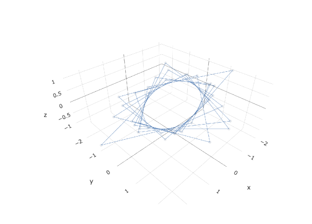
Figure 6: Typical path of the process $y_{\mathrm{L}}(t)$.

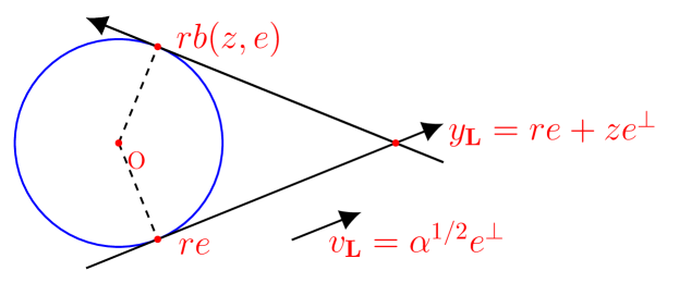
Figure 7: Trajectory of $y_{\mathrm{L}}(t)$

Proposition 5.2.

Assuming that Assumption 5.1 holds, and given the vectors $y_{\mathrm{L}}(0)$ and $v_{\mathrm{L}}(0)$, which are assumed to be linearly independent, we define $\Pi$ as the oriented hyperplane spanned by these vectors. Then, we can assert that $(z(t),e(t))$ forms an ergodic Markov process with extended generator $H$, and its invariant distribution is $\mathcal{N}(0,1)\otimes\mathcal{U}(\mathbb{S})$.

Proof.

Observe that linearly independence implies $\alpha>0$. Let $0=\tau_{0}<\tau_{1}<\cdots$ be the jump times of the Markov process $(y_{\mathrm{L}}(t),v_{\mathrm{L}}(t))$. For each $n=0,1,\ldots$, $v_{\mathrm{L}}(t)=v_{\mathrm{L}}(\tau_{n})$ and

$$y_{\mathrm{L}}(t)=y_{\mathrm{L}}(\tau_{n})+v_{\mathrm{L}}(\tau_{n})~{}(t-\tau_{n})$$

forms a line segment in each time interval $t\in[\tau_{n},\tau_{n+1})$. By the constraint equation (5.3),

$$r^{2}=|y_{\mathrm{L}}|^{2}-(v_{\mathrm{L}}^{\top}y_{\mathrm{L}})^{2}/|v_{\mathrm{L}}|^{2}\quad\Longrightarrow\quad|y_{\mathrm{L}}|\geq r$$

and equality holds if and only if $z=y_{\mathrm{L}}^{\top}v_{\mathrm{L}}=0$. Therefore, the line segment is tangent to the circle of radius $r$. Also, since

$$z(t)=z(\tau_{n})+(t-\tau_{n})\alpha^{1/2},\quad t\in[\tau_{n},\tau_{n+1})$$

and $z(\tau_{n})=-z(\tau_{n}-)<0$, the tangency point $z(t)=0$ is included in each line segment. From this observation, for each line segment, we can define the orientation, clockwise or counterclockwise, by observing the direction at the tangency point.

We claim that the orientation of all line segments are consistent. Otherwise, there exists a set of line segments with differing orientations, such as $(y_{\mathrm{L}}(t):\tau_{n}\leq t<\tau_{n+1})$ and $(y_{\mathrm{L}}(t):\tau_{n+1}\leq t<\tau_{n+2})$. At $y(\tau_{n+1})$, there are two tangent lines to the two-dimensional circle of radius $r$. If the two line segments are on different tangent lines, then the orientation must be the same, given that the path $(y_{\mathrm{L}}(t):\tau_{n}\leq t<\tau_{n+2})$ is connected. Thus, if orientations are different, the two line segments are on the same tangent line, and the orientations of the two line segments must have opposite signs, i.e. $v_{\mathrm{L}}(\tau_{n+1}-)=-v_{\mathrm{L}}(\tau_{n+1})$. This can only occur when $v_{\mathrm{L}}(t)/|v_{\mathrm{L}}(t)|=y_{\mathrm{L}}(t)/|y_{\mathrm{L}}(t)|$ at $t=\tau_{n+1}-$. However by turning back the time it implies linearly dependence of $v_{\mathrm{L}}(0)$ and $y_{\mathrm{L}}(0)$ which contradicts the initial assumption.

Observe that

$$e^{\perp}:=\alpha^{-1/2}~{}v_{\mathrm{L}}\quad\Longrightarrow\quad z=y_{\mathrm{L}}^{\top}e^{\perp}\ \mathrm{and}\ e=r^{-1}(y_{\mathrm{L}}-z~{}e^{\perp})\quad\Longrightarrow\quad e\perp e^{\perp}.$$

The unit vector $e^{\perp}$ is solely determined by the vector $e$ together with the orientation of the segments. By construction, $e\perp v_{\mathrm{L}}$ and $r~{}e=y_{\mathrm{L}}-zv_{\mathrm{L}}/|v_{\mathrm{L}}|$ is on the line segment. Thus $r~{}e$ is the point of tangency. See Figure 7. For given $\Pi$, $\alpha,\beta$ and the orientation of the process, there is a map $\varphi(z,e)=(y_{\mathrm{L}},v_{\mathrm{L}})$ from $\mathbb{R}\times\mathbb{S}$ to $\mathbb{R}^{l}\times\mathbb{R}^{l}$ defined by

$$v_{\mathrm{L}}=\alpha^{1/2}e^{\perp},\quad\ y_{\mathrm{L}}=re+ze^{\perp}.$$

If there is a reflection jump event at $t>0$, then $e^{\perp}$ will jump to

$$(e^{\perp})^{*}=e^{\perp}-2\frac{v_{\mathrm{L}}^{\top}y_{\mathrm{L}}}{|v_{\mathrm{L}}|}\frac{y_{\mathrm{L}}}{|y_{\mathrm{L}}|^{2}}=\frac{-2rz}{r^{2}+z^{2}}e+\frac{r^{2}-z^{2}}{r^{2}+z^{2}}e^{\perp}$$

where we used $|y_{\mathrm{L}}|^{2}=r^{2}+z^{2}$. Also, $z$ jumps to $-z$, and $e$ jumps to

$$b(z,e)=r^{-1}(y_{\mathrm{L}}-(-z)~{}(e^{\perp})^{*})=\frac{r^{2}-z^{2}}{r^{2}+z^{2}}e+\frac{2rz}{r^{2}+z^{2}}e^{\perp}.$$ (5.6)

Since $(y_{\mathrm{L}}(t),v_{\mathrm{L}}(t))$ is a Markov process, $(z(t),e(t))$ is also a Markov process. The Markov process $(z(t),e(t))$ is ergodic if there is an invariant probability measure by Proposition 5.7 below and Theorem 1 of [19]. We show that the invariant probability measure is $\mathcal{N}(0,1)\otimes\mathcal{U}(\mathbb{S})$. To see this, observe that the extended generator of the Markov process $(z(t),e(t))$ is

$$\widetilde{H}f(z,e)=\mathcal{L}_{0}(f\circ\varphi^{-1})(\varphi(z,e))$$

since for $Y_{t}:=(z(t),e(t))$, $X_{t}=\varphi(X_{t})=(y_{\mathrm{L}}(t),v_{\mathrm{L}}(t))$ and $g=f\circ\varphi^{-1}$, the process

$$M_{T}:=f(Y_{T})-f(Y_{0})-\int_{0}^{T}(\widetilde{H}f)(Y_{t})\mathrm{d}t =g(X_{T})-g(X_{0})-\int_{0}^{T}(\mathcal{L}_{0}g)(X_{t})\mathrm{d}t$$

is a local martingale when $g$ is the domain of the extended generator of $\mathcal{L}_{0}$. We see that the extended generator $\widetilde{H}$ coincides $H$ in (5.4). Observe that we have the expression

$$(z,e)=\varphi^{-1}(y_{\mathrm{L}},v_{\mathrm{L}})=(\alpha^{-1/2}~{}y_{\mathrm{L}}^{\top}v_{\mathrm{L}},r^{-1}(y_{\mathrm{L}}-(\alpha^{-1/2}y_{\mathrm{L}}^{\top}v_{\mathrm{L}})~{}(\alpha^{-1/2}v_{\mathrm{L}}))).$$

By differentiating both sides of the equation, we obtain

$$v_{\mathrm{L}}^{\top}\partial_{y_{\mathrm{L}}}z=\alpha^{1/2},\ \quad v_{\mathrm{L}}^{\top}\partial_{y_{\mathrm{L}}}e=0.$$

Together with the fact that the $(z,e)$ jumps to $(-z,b(z,e))$ at the reflection jump, the expression (5.4) follows. By integration by parts formula, we have

$$\int_{-\infty}^{\infty}\left\{\partial_{z}f(z,e)+z_{+}(f(-z,e)-f(z,e))\right\}\phi(z)\mathrm{d}z=\int_{-\infty}^{\infty}\left\{\partial_{z}f(z,e)-zf(z,e)\right\}\phi(z)\mathrm{d}z=0$$

for any absolutely continuous function $f(\cdot,e)$ such that $\int|\partial_{z}f(z,e)|\phi(z)\mathrm{d}z<\infty$ for each $e\in\mathbb{S}$. On the other hand,

$$\int_{\mathbb{S}}f(-z,b(z,e))\mathrm{d}e=\int_{\mathbb{S}}f(-z,e)\mathrm{d}e.$$

Therefore the expectation of $Hf$ with respect to $\mathcal{N}(0,1)\otimes\mathcal{U}(\mathbb{S})$ is always $0$. Hence the claim follows from Theorem 21 and Corollary 22 of [12]. ∎

Let $\tau_{i}$ be the $i$-th reflection jump time of $(z(t),e(t))$ for $i\geq 1$, and let $\tau_{0}=0,z(0)=z_{0}$. Let

$$\omega_{n}=\tau_{n}+2\sum_{m=1}^{n-1}(-1)^{m}\tau_{n-m}+(-1)^{n+1}z_{0},\quad\theta_{n}=\arctan\omega_{n}\ (n=1,2,\ldots).$$ (5.7)

Figure 8 illustrates the relation of the variables when $\alpha=\beta=1$. In this case, $z(t)$ is the distance from the tangency point on a line segment to the process $y_{\mathrm{L}}(t)$.

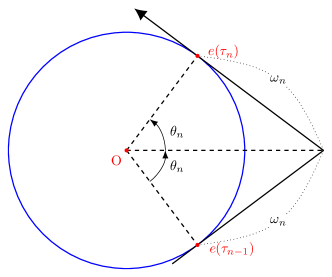
Figure 8: Relation among $\omega_{n},\tau_{n}$ and $\theta_{n}$ when $\alpha=\beta=1$.

Lemma 5.3.

Assume that $\alpha=\beta=1$. Then

$$z(\tau_{n}-)=\omega_{n}\ (n\in\mathbb{N})$$ (5.8)

are independent and identically distributed and $\mathbb{P}(w_{n}>x)=\exp(-x^{2}/2)$ for $x>0$. Also,

$$\arccos(e(\tau_{n})^{\top}e(\tau_{n-1}))=2\theta_{n}\ (n=1,2,\ldots).$$

In particular,

$$\arccos(e(\tau_{n})^{\top}e(0))=2\sum_{k=1}^{n}\theta_{k}\ (n=1,2,\ldots).$$

Proof.

The process $z$ is completely determined by the stopping times. In particular, we have

$$z(\tau_{n}-)=\begin{cases}-z(\tau_{n-1}-)+(\tau_{n}-\tau_{n-1})&n\geq 2\\ z_{0}+\tau_{1}&n=1.\end{cases}$$

since $z^{\prime}(t)=1$ for $t\neq\tau_{n}\ (n=1,2,\ldots)$ and $z(\tau_{n})=-z(\tau_{n}-)$. See Figure 9. Therefore, by inductive argument, we have $z(\tau_{n}-)=\omega_{n}$. Since $w_{n}$ denotes the time elapsed between the moment when $z(t)$ hits zero at time $t=\tau_{n-1}+z(t_{n-1})$ and the subsequent jump, and $z(t)_{+}$ represents the intensity function, we can draw the following conclusion:

$$\mathbb{P}(w_{n}>x)=\exp\left(-\int_{0}^{x}y~{}\mathrm{d}y\right)=\exp(-x^{2}/2).$$

Thus the first claim follows. For the second claim, at the jump time $\tau_{n}$,

$$(\ref{eq:e_jump})\quad\Longrightarrow e(\tau_{n})^{\top}e(\tau_{n}-)=b(z(\tau_{n}-),e(\tau_{n}-))^{\top}e(\tau_{n}-)=\frac{1-z(\tau_{n}-)^{2}}{1+z(\tau_{n}-)^{2}}.$$

Therefore

$$e(\tau_{n})^{\top}e(\tau_{n-1})=e(\tau_{n})^{\top}e(\tau_{n}-)=\frac{1-\omega_{n}^{2}}{1+\omega_{n}^{2}}=\frac{1-\tan\theta_{n}^{2}}{1+\tan\theta_{n}^{2}}=\cos 2\theta_{n}.$$

Thus the second claim follows. The last claim follows from the fact that the process $y_{\mathrm{L}}(t)$ .keeps its orientation. ∎

Let $P_{t}$ be the Markov semigroup of $H$.

Lemma 5.4.

Assume that $\alpha=\beta=1$. There is a coupling of measures $P_{t}((z_{0},e_{0}),\cdot)$ and $P_{t}((z_{0}^{*},e_{0}^{*}),\cdot)$ such that the first hitting time $T_{D_{0}}$ of

$$D_{0}=\{(z,e,z^{*},e^{*})\in(\mathbb{R}\times\mathbb{S})^{2}:z=z^{*}=0\}$$

is finite with positive probability.

Proof.

Let $(z(t),e(t))$ and $(z^{*}(t),e^{*}(t))$ be the realisation of the coupling. The process $z$ is completely determined by the stopping times. In particular, as described in Figure 9,

$$z(t)=\begin{cases}t+z_{0}&\ t\in[0,\tau_{1})\\ t-(z_{0}+2\tau_{1})&\ t\in[\tau_{1},\tau_{2})\end{cases}\quad\Longrightarrow\quad z(\xi)=0,\ \mathrm{where}\ \xi=z_{0}+2\tau_{1}$$

Similarly, $z^{*}(\xi^{*})=0$, where $\xi^{*}=z_{0}^{*}+2\tau_{1}^{*}$.

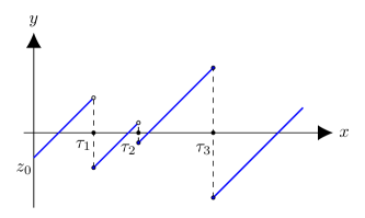
Figure 9: Path of $z(t)$ when $\alpha=\beta=1$

We begin by defining $\mathbb{Q}$ as the maximal coupling of $\xi$ and $\xi^{*}$. Using this coupling, we construct a coupling of Markov processes, denoted by $\mathbb{P}$, by taking $(\xi,\xi^{*})\sim\mathbb{Q}$ along with the conditionally independent realisations of stopping times given $\xi$ and $\xi^{*}$. From this construction, we obtain

$$\mathbb{P}\left(T_{D_{0}}<\infty\right)~{}\geq~{}\mathbb{P}(\xi=\xi^{*})=\mathbb{Q}(\xi=\xi^{*})=1-\|\mathcal{L}(\xi)-\mathcal{L}(\xi^{*})\|_{\mathrm{TV}}.$$

The left-hand side equals to $0$ if and only if the laws of $\xi$ and $\xi^{*}$ are mutually singular. However, since $\tau_{1}$ has a positive probability density on $[(-z_{0})+,\infty)$, it follows that the random variable $\xi$ has a positive probability density on $[|z_{0}|,\infty)$, and similarly, $\xi^{*}$ has a positive probability density on $[|z_{0}^{*}|,\infty)$. Thus, the laws of $\xi$ and $\xi^{*}$ cannot be mutually singular, implying that the stopping time $T_{D_{0}}$ is finite with positive probability." ∎

Lemma 5.5.

Assume that $\alpha=\beta=1$. If $e_{0}+e_{0}^{*}\neq 0$, there is a coupling of measures $P_{t}((0,e_{0}),\cdot)$ and $P_{t}((0,e_{0}^{*}),\cdot)$ such that the first hitting time $T_{D}$ of

$$D=\{(z,e,z^{*},e^{*})\in(\mathbb{R}\times\mathbb{S})^{2}:(z,e)=(z^{*},e^{*})\}$$

is finite with positive probability.

Proof.

The process $z$ starting from $z(0)=0$ satisfies

$$z(t)=\begin{cases}t&\ t\in[0,\tau_{1})\\ t-2\tau_{1}&\ t\in[\tau_{1},\tau_{2})\\ t-2(\tau_{2}-\tau_{1})&\ t\in[\tau_{2},\tau_{3})\end{cases}\quad\Longrightarrow\quad z(\xi)=0,\ \mathrm{where}\ \xi=2(\tau_{2}-\tau_{1})\in[\tau_{2},\tau_{3}).$$ (5.9)

Similarly, $z^{*}(\xi^{*})=0$ for $\xi^{*}=2(\tau_{2}^{*}-\tau_{1}^{*})$. Let $\epsilon=\arccos((e_{0}^{*})^{\top}e_{0})$ be the angle between the initial tangency points of two Markov processes. Without loss of generality, we can assume that $\epsilon\in(0,\pi)$. By Lemma 5.3, the angle of $e(\xi)$ and $e^{*}(\xi^{*})$ from $e(0)$ are twice of

$$\theta=\theta_{1}+\theta_{2},\quad\theta^{*}=\theta_{1}^{*}+\theta_{2}^{*}+\epsilon/2$$

where $\theta_{n}$ is defined in (5.7), and $\theta^{*}_{n}$ is as in (5.7), replacing $\tau_{j}$ by $\tau_{j}^{*}$. Thus

$$(\xi,\theta)=(\xi^{*},\theta^{*})~{}\Longrightarrow~{}(z(\xi),e(\xi))=(z^{*}(\xi),e^{*}(\xi))~{}\Longrightarrow~{}T_{D}<\infty.$$

As in the previous lemma, the proof will be completed if we can show that the laws of $(\xi,\theta)$ and $(\xi^{*},\theta^{*})$ are not mutually singular.

By (5.7) and (5.8),

$$\begin{cases}(\xi/2)=\omega_{1}+\omega_{2},\\ (\xi^{*}/2)=\omega_{1}^{*}+\omega_{2}^{*},\end{cases}\begin{cases}\theta=\arctan\omega_{1}+\arctan\omega_{2},\\ \theta^{*}=\arctan\omega_{1}^{*}+\arctan\omega_{2}^{*}+\epsilon/2\end{cases}$$

where $\omega_{n}=z(\tau_{n}-)$ and $\omega_{n}^{*}=z^{*}(\tau_{n}^{*}-)$. Both $(w_{n})_{n}$ and $(w_{n}^{*})_{n}$ are independent and identically distributed with positive probability density on $\mathbb{R}_{+}$. Thus, conditioned on $\xi$ and $\xi^{*}$, the variables $x=\omega_{1}/(\omega_{1}+\omega_{2})$ and $x^{*}=\omega_{1}^{*}/(\omega_{1}^{*}+\omega_{2}^{*})$ are independent and identically distributed and have positive probability distribution function on the interval $[0,1]$.

For given $\xi$ the map

$$f(x)=\arctan(x\xi/2)+\arctan((1-x)\xi/2)$$ (5.10)

is symmetric about $x=1/2$, and it is monotone increasing in the interval $[0,1/2]$ since $f^{\prime}(s)=(\xi/2)/(1+(x\xi/2)^{2})-(\xi/2)/(1+((1-x)\xi/2)^{2})>0$. Thus

$$\arctan\xi/2=f(0)\leq f(x)\leq f(1/2)=2\arctan\xi/4.$$

Therefore $\theta=f(x)$ has a positive probability density function on $[\arctan\xi/2,2\arctan\xi/4]$, and $\theta^{*}=\epsilon+f(x^{*})$ has a positive probability density function on $[\epsilon/2+\arctan\xi/2,\epsilon/2+2\arctan\xi/4]$. These measures are not mutually singular if

$$\epsilon/2+\arctan\xi/2<2\arctan\xi/4.$$

The function $g(\xi)=2\arctan\xi/4-\arctan\xi/2$ is a monotone increasing function and $\sup_{\xi\in\mathbb{R}_{+}}g(\xi)=\pi/2$. Thus if $\epsilon<\pi$, then the laws of $\theta$ and $\theta^{*}$ given $\xi=\xi^{*}$ are not mutually singular if we take $\xi=\xi^{*}$ large enough. Thus $T_{D}$ is finite with a positive probability. ∎

Lemma 5.6.

Assume that $\alpha=\beta=1$. If $e+e^{*}=0$, there is a coupling of measures $P_{t}((0,e_{0}),\cdot)$ and $P_{t}((0,e_{0}^{*}),\cdot)$ such that the first hitting time $T_{D}$ of

$$D^{\prime}_{0}=\{(z,e,z^{*},e^{*})\in(\mathbb{R}\times\mathbb{S})^{2}:(z,e)=(z^{*},e^{*}),e+e^{*}\neq 0\}$$

is finite with positive probability.

Proof.

Let $\theta_{n}$ and $\omega_{n}$ as in (5.7), and let $\theta_{n}^{*}$ and $\omega_{n}^{*}$ be the same replacing $\tau_{n}$ by $\tau_{n}^{*}$. Then

$$\xi:=2(\tau_{2}-\tau_{1})=2(\omega_{1}+\omega_{2}),\ \xi^{*}:=2\tau_{1}^{*}=2\omega_{1}~{}\overset{(\ref{eq:zprocess})}{\Longrightarrow}~{}z(\xi)=z^{*}(\xi^{*})=0.$$

Let $\mathbb{Q}$ be maximal coupling of the laws of $\xi$ and $\xi^{*}$. Then $\mathbb{Q}(\xi=\xi^{*})>0$. The coupling of Markov processes, denoted by $\mathbb{P}$, is constructed by $(\xi,\xi^{*})\sim\mathbb{Q}$ together with the conditionally independent realisations of stopping times given $\xi$ and $\xi^{*}$. The variable $x=\omega_{1}/(\omega_{1}+\omega_{2})$ has a continuous probability density function on $[0,1]$ under $\mathbb{P}$ given $\xi$ and $\xi^{*}$.

On the other hand, by Lemma 5.3,

$$\arccos e(\xi)^{\top}e(0)=2\theta_{2}+2\theta_{1},\ \arccos e^{*}(\xi^{*})^{\top}e^{*}(0)=2\theta_{1}^{*},$$

$$\quad\overset{\mathrm{if}\ \xi=\xi^{*}}{\Longrightarrow}\quad\arccos e(\xi)^{\top}e^{*}(\xi)=2(\theta_{1}+\theta_{2}-\theta_{1}^{*})+\pi.$$

Since the arctangent function is a subadditive function on $\mathbb{R}_{+}$, we have

$$\xi=\xi^{*}~{}\Longrightarrow~{}\theta_{1}+\theta_{2}-\theta_{1}^{*} \overset{(\ref{eq:bpstheta})}{=}\arctan\omega_{1}+\arctan\omega_{2}-\arctan\omega_{1}^{*}$$

$$~{}=\arctan(x\xi/2)+\arctan((1-x)\xi/2)-\arctan(\xi/2)>0$$

$$\Longrightarrow~{}e(\xi)+e^{*}(\xi)\neq 0$$

where we used the fact that $f(x)$ defined in (5.10) is monotone increasing. Thus $\xi=\xi^{*}\Longrightarrow(z(\xi),e(\xi),z^{*}(\xi),e^{*}(\xi))\in D_{0}^{\prime}$. Hence $\mathbb{P}(T_{D_{0}^{\prime}}<\infty)\geq\mathbb{Q}(\xi=\xi^{*})>0$. ∎

Proposition 5.7.

Let $P_{t}$ be the Markov kernel of $(z(t),e(t))$. Then for $(z,e),(z^{*},e^{*})\in\mathbb{R}\times\mathbb{S}$, there exists $T>0$ such that

$$P_{t}((z,e),\cdot)\not\perp P_{t}((z^{*},e^{*}),\cdot)$$ (5.11)

for all $t\geq T$.

Proof.

Let $w(t)=(z(t),e(t),z^{*}(t),e^{*}(t))$ and let $(\mathcal{F}_{t})$ be the filtration. We assume $\alpha=\beta=1$. This is always possible by state scaling and time scaling. Without loss of generality, we can assume that the process $z$ is counter clockwise and all angles in this proof will be measured in this orientation.

We use the couplings in Lemmas 5.4, 5.5, and 5.6, as described in equation (5.12). Specifically, we first use the coupling in Lemma 5.5 for $(z,e)\in\mathbb{R}\times\mathbb{S}$ until it hits $D_{0}$. If it is in $(D_{0}^{\prime})^{c}$, we then use Lemma 5.4 until it hits $D_{0}^{\prime}$. Finally, from $D_{0}$ until it reaches $D$, we use the coupling in Lemma 5.6:

$$(z,e)\overset{\mathrm{Lemma}\ \ref{lem:bpsd}}{\Longrightarrow}D_{0}\quad(\mathrm{if}\ e+e^{\prime}=0\ \overset{\mathrm{Lemma}\ \ref{lem:bpsdperp}}{\Longrightarrow}D_{0}^{\prime})\quad\overset{\mathrm{Lemma}\ \ref{lem:bpsd0}}{\Longrightarrow}\quad D$$ (5.12)

By Markov property, the constructed probability measure satisfies $\mathbb{P}(T_{D}<\infty)>0$. Hence, by modifying the processes so that they are coincides after $t=T_{D}$, we can show that there exists $T>0$ such that $0<\mathbb{P}(T_{D}<T)=1-\|P_{T}((z,e),\cdot)-P_{T}((z^{*},e^{*}),\cdot)\|_{\mathrm{TV}}$. Therefore, the claim follows. ∎

Corollary 5.8.

Let $y_{\mathrm{L}}(0),v_{\mathrm{L}}(0)\in\mathbb{R}^{\mathrm{L}}$ be fixed constants such that the two vectors are linearly independent. Then

$$\mathbb{E}\left[\frac{(v_{\mathrm{L}}(t)^{\top}y_{\mathrm{L}}(t))_{+}^{2}}{|y_{\mathrm{L}}(t)|^{2}}\right]=\mathbb{E}\left[\frac{\alpha~{}z(t)_{+}^{2}}{\beta/\alpha+z(t)^{2}}\right]\longrightarrow_{t\rightarrow\infty}c(\alpha,\beta)$$

where, for $r=(\beta/\alpha)^{1/2}$,

$$c(\alpha,\beta)=\alpha-\sqrt{2\pi}~{}\alpha re^{r^{2}/2}\Phi(-r)=\alpha\left[1-r\frac{\Phi(-r)}{\phi(r)}\right]$$ (5.13)

where $\Phi$ is the cumulative distribution function of the normal distribution.

Proof.

The equation (5.3) yields the first equation. Since the invariant measure of $z(t)$ is the standard normal distribution, by the law of large numbers and by Proposition 5.2, the expectation is

$$\int_{\mathbb{R}}\frac{\alpha x^{2}}{r^{2}+x^{2}}\phi(x)\mathrm{d}x=\alpha-\alpha r^{2}~{}\int_{\mathbb{R}}\frac{1}{r^{2}+x^{2}}\phi(x)\mathrm{d}x.$$

Since the characteristic function of the probability density function $\phi(x)$ of the standard normal distribution is $\sqrt{2\pi}\phi(x)$, we have

$$\int_{\mathbb{R}}\frac{1}{r^{2}+x^{2}}\phi(x)\mathrm{d}x =(2\pi)^{-1/2}\int_{\mathbb{R}}\int_{\mathbb{R}}\frac{1}{r^{2}+x^{2}}e^{\mathbf{i}xu}\phi(u)\mathrm{d}x\mathrm{d}u$$

$$=(2\pi)^{-1/2}r^{-1}\int_{\mathbb{R}}\int_{\mathbb{R}}\frac{1}{1+x^{2}}e^{\mathbf{i}xur}\phi(u)\mathrm{d}x\mathrm{d}u$$

$$=(\pi/2)^{1/2}r^{-1}\int_{\mathbb{R}}e^{-|u|r}\phi(u)\mathrm{d}u$$

where we used the fact that the characteristic function of the Cauchy distribution $\pi^{-1}(1+x^{2})^{-1}\mathrm{d}x$ is $\exp(-|x|)$. This expectation is

$$2~{}(\pi/2)^{1/2}r^{-1}\int_{0}^{\infty}e^{-ur}\phi(u)\mathrm{d}u=2~{}(\pi/2)^{1/2}r^{-1}~{}\Phi(-r)e^{r^{2}/2}.$$

This proves the claim. ∎

5.2 Averaging of the bouncy particle sampler

5.2.1 First convergence regime of the bouncy particle sampler

Let $\xi_{*}^{\epsilon}(t)=(y_{*}^{\epsilon}(t),v_{*}^{\epsilon}(t))$ be the $\epsilon$-time scaled Markov process of (3.5) corresponding to the extended generator

$$\mathcal{L}_{*}^{\epsilon}=\epsilon~{}((\Lambda^{\epsilon})^{-1}v)^{\top}\partial_{y}+\epsilon~{}(v^{\top}(\Lambda^{\epsilon})^{-1}y)_{+}(\mathcal{B}^{\epsilon}-\mathrm{id})+\epsilon~{}\rho~{}(\mathcal{R}-\mathrm{id}).$$

First we prove the convergence $\xi_{*}^{\epsilon}\longrightarrow\xi_{0}$ in Skorokhod topology where $\xi_{0}(t)=(y_{0}(t),v_{0}(t))$ is the Markov process with extended generator (5.2). We assume that $\xi_{0}(0)=\xi^{\epsilon}_{*}(0)$.

Proposition 5.9 (Fast convergence regime).

As $\epsilon\rightarrow 0$, the Markov process $\xi^{\epsilon}_{*}$ starting from $(x,v)\in\mathbb{R}^{d}\times\mathbb{R}^{d}$ converges to another Markov process of (5.2) in Skorokhod topology.

Proof.

We assume that $\xi_{*}^{\epsilon}(0)=\xi_{0}(0)$ and consider the initial points as fixed constants. By Lemma VI.3.31, without loss of generality, we can assume that $\rho=0$, since the refreshment jump occurs in the time interval $[0,T]$ with probability $1-\exp(-\epsilon\rho T)$, which converges to $0$ for $\epsilon\rightarrow 0$. The reflection jump does not change the size of the velocity variable, that is, $|v_{*}^{\epsilon}(t)|=|v_{0}(0)|$. Therefore, we have a local uniform bound

$$y_{*}^{\epsilon}(t)=y_{0}(0)+\epsilon~{}\int_{0}^{t}(\Lambda^{\epsilon})^{-1}v_{*}^{\epsilon}(s)\mathrm{d}s\quad\Longrightarrow\quad|y_{*}^{\epsilon}(t)-y_{0}(0)| \leq\epsilon~{}\|(\Lambda^{\epsilon})^{-1}\|~{}|v_{0}(0)|~{}t$$

$$\leq(\epsilon\|\Lambda_{\mathrm{K}}^{-1}\|+\|\Lambda_{\mathrm{L}}^{-1}\|)~{}|v_{0}(0)|~{}t.$$

A similar inequality holds for $\xi_{0}$. In particular, the Markov processes are bounded on any finite interval $[0,T]$. Therefore, we can apply Theorem IX.3.27 of [18], which is the limit theorem for bounded processes.

By Dynkin’s formula, for $h\in C^{1}(\mathbb{R}^{d}\times\mathbb{R}^{d})$, the compensator associated to the jumps of $\xi_{*}^{\epsilon}$ is characterised by

$$\int_{\mathbb{R}^{d}\times\mathbb{R}^{d}}h(\xi)\nu_{t}^{\epsilon}(\mathrm{d}\xi):=\int_{0}^{t}\lambda^{\epsilon}(\xi_{*}^{\epsilon}(s))~{}h(0,(\mathcal{B}^{\epsilon}(y^{\epsilon}_{*}(s))-\mathrm{id})v_{*}^{\epsilon}(s))\mathrm{d}s$$

where

$$\lambda^{\epsilon}(\xi)=\epsilon~{}(v^{\top}(\Lambda^{\epsilon})^{-1}y)_{+}.$$

Write $\nu_{t}$ for the compensator associated to the jumps of $\xi_{0}$. Since each jump size is bounded above by $2|v_{0}(0)|$, we have

$$a>2|v_{0}(0)|~{}\Longrightarrow~{}\int_{\mathbb{R}^{d}}|v|^{2}~{}1_{\{|v|>a\}}\nu_{t}^{\epsilon}(\{0\}\times\mathrm{d}v)=0~{}\Longrightarrow~{}\mathrm{(3.29)}.$$

Similarly, condition (ii), i.e., 3.28 and condition 3.24 are satisfied. We have

$$b^{\epsilon}(\xi) :=\left(\epsilon(\Lambda^{\epsilon})^{-1}v,\quad\epsilon~{}(v^{\top}(\Lambda^{\epsilon})^{-1}y)_{+}(B^{\epsilon}(y)-\mathrm{id})v\right)$$

$$\quad\quad\quad\quad\quad\longrightarrow_{\epsilon\rightarrow 0}\left(\left(0,\Lambda_{\mathrm{L}}^{-1}v_{\mathrm{L}}\right),\left(0,(v_{\mathrm{L}}^{\top}\Lambda_{\mathrm{L}}^{-1}y_{\mathrm{L}})_{+}(B^{0}(y)-\mathrm{id})v_{\mathrm{L}}\right)\right)=:b(\xi)$$

locally uniformly in $\xi=(y,v)$. Let

$$B_{t}^{\prime\epsilon}:=\int_{0}^{t}b^{\epsilon}(\xi_{*}^{\epsilon}(s))\mathrm{d}s,\quad B_{t}^{\prime}:=\int_{0}^{t}b(\xi_{0}(s))\mathrm{d}s.$$

Then

$$B_{t}^{\prime\epsilon}-B_{t}^{\prime}\circ\xi^{\epsilon}_{*}\longrightarrow_{\epsilon\rightarrow 0}0~{}\Longrightarrow~{}\mathrm{[Sup-}\beta^{\prime}_{7}\mathrm{]}$$

where $B_{t}^{\prime}\circ\xi_{*}^{\epsilon}$ is the process $B_{t}^{\prime}$ replacing $\xi$ by $\xi_{*}^{\epsilon}$. Similarly,

$$\tilde{C}_{t}^{\prime}:=\int_{\mathbb{R}^{d}}v^{\otimes 2}\nu_{t}(\{0\}\times\mathrm{d}v)\quad \Longrightarrow\quad\tilde{C}^{\prime\epsilon}_{t}:=\int_{\mathbb{R}^{d}}v^{\otimes 2}\nu_{t}^{\epsilon}(\{0\}\times\mathrm{d}v)\longrightarrow_{\epsilon\rightarrow 0}\widetilde{C}_{t}^{\prime}\circ\xi_{*}^{\epsilon}$$

$$\Longrightarrow\mathrm{[}\gamma_{7}^{\prime}\mathrm{-D]}$$

where $\widetilde{C}_{t}^{\prime}\circ\xi_{*}^{\epsilon}$ is the process $\widetilde{C}_{t}$ replacing $\xi$ by $\xi_{*}^{\epsilon}$. The same convergence holds by replacing $v^{\otimes 2}$ by $g$ where $g:\mathbb{R}^{d}\rightarrow\mathbb{R}$ is a continuous bounded function which is $0$ around $0\in\mathbb{R}^{d}$. This yields [$\delta_{7,1}$-D]. Other regularity conditions (i), (iv) and (v) can easily be verified.

The argument used in Theorem 4.6 is used to establish both the uniqueness of the corresponding martingale problem in equation (5.2) and condition (iii). ∎

5.2.2 Reparametrisation and expansion of the generator

We contemplate the reparametrisation of $(y,v)$ in order to facilitate the analysis. Let

$$x=(y_{\mathrm{K}},v_{\mathrm{K}},\alpha,\beta),\quad\zeta=(z,e,x)=(z,e,y_{\mathrm{K}},v_{\mathrm{K}},\alpha,\beta)$$

and let $\psi,\pi$ be projections such that

$$(y,v)\quad\overset{\pi}{\longrightarrow}\quad\zeta=(z,e,x)\quad\overset{\psi}{\longrightarrow}\quad x=(y_{\mathrm{K}},v_{\mathrm{K}},\alpha,\beta)$$ (5.14)

where $\alpha$ and $\beta$ are as in (5.3). Let $\Pi$ be the two-dimensional hyperplane spanned by $y_{\mathrm{L}}(0)$ and $v_{\mathrm{L}}(0)$. The processes $y_{\mathrm{L}}(t)$ and $v_{\mathrm{L}}(t)$ remain on the hyperplane until the next refreshment jump. Let $\gamma\in\{-1,+1\}$ be the orientation of the hyperplane $\Pi$. When $\Pi$ and $\gamma$ are fixed, then $(y,v)$ and $\zeta$ have a one-to-one correspondence. Since $\Pi$ and $\gamma$ are fixed between the refreshment jump times, we focus on the variable $\zeta$. Let $r=\sqrt{\beta/\alpha}$.

We are now going to rewrite the generator $\mathcal{L}^{\epsilon}$ using the reparametrisation. With the reparametrisation $\pi:(y,v)\mapsto\zeta$ we have the correspondences

$$\begin{cases}y^{\prime}=(\Lambda^{\epsilon})^{-1}v&\mapsto\quad z^{\prime}=\epsilon^{-1}\alpha^{1/2},\quad y_{\mathrm{K}}^{\prime}=\Lambda_{\mathrm{K}}^{-1}v_{\mathrm{K}}\\ (v^{\top}(\Lambda^{\epsilon})^{-1}y)_{+}&\mapsto\quad(\epsilon^{-1}\alpha^{1/2}~{}z+v_{\mathrm{K}}^{\top}\Lambda_{\mathrm{K}}^{-1}y_{\mathrm{K}})_{+}\\ \mathcal{B}^{\epsilon}f(\xi)&\mapsto\quad\widetilde{\mathcal{B}}^{\epsilon}f(\zeta):=\mathcal{B}^{\epsilon}(f)(\pi^{-1}\zeta)\\ \mathcal{R}f(\xi)&\mapsto\quad\widetilde{\mathcal{R}}f(\zeta):=\mathcal{R}(f)(\pi^{-1}\zeta).\end{cases}$$

The operator $\widetilde{\mathcal{B}}^{0}$ is given as the pullback of the reflection

$$\zeta=(z,e,x)\mapsto(-z,b(z,e),x).$$

Let $n(v)=v/|v|$ for a vector $v\neq 0$. The refresh operator $\widetilde{\mathcal{R}}$ is given as the jump from $\zeta$ to $\zeta^{*}$ as follows, where $v^{*}=(v_{\mathrm{K}}^{*},v_{\mathrm{L}}^{*})\sim\mathcal{N}(0,I_{d})$:

$$\begin{split}&\zeta=\begin{pmatrix}z\\ e\\ y_{\mathrm{K}}\\ v_{\mathrm{L}}\\ \alpha\\ \beta\end{pmatrix}\quad\mapsto\quad\zeta^{*}=\begin{pmatrix}z^{*}\\ n(w^{*})\\ y_{\mathrm{K}}\\ v_{\mathrm{K}}^{*}\\ |v_{\mathrm{L}}^{*}|^{2}\\ |v_{\mathrm{L}}^{*}|^{2}~{}|w^{*}|^{2}-((v_{\mathrm{L}}^{*})^{\top}w^{*})^{2}\end{pmatrix}\\ &\quad\quad\ \mathrm{where}\ z^{*}=n(v_{\mathrm{L}}^{*})^{\top}y_{\mathrm{L}},\quad w^{*}=(1-n(v_{\mathrm{L}}^{*})~{}n(v_{\mathrm{L}}^{*})^{\top})~{}y_{\mathrm{L}}.\end{split}$$ (5.15)

The generator $\mathcal{L}^{\epsilon}$ now becomes

$$\mathcal{L}^{\epsilon}f(z,e,x) =\epsilon^{-1}\alpha^{1/2}\partial_{z}f(z,e,x)+(\Lambda_{\mathrm{K}}^{-1}v_{\mathrm{K}})^{\top}\partial_{y_{\mathrm{K}}}f(z,e,x)$$

$$\quad+(\epsilon^{-1}\alpha^{1/2}~{}z+v_{\mathrm{K}}^{\top}\Lambda_{\mathrm{K}}^{-1}y_{\mathrm{K}})_{+}(\widetilde{\mathcal{B}}^{\epsilon}-\mathrm{id})f(z,e,x)+\rho~{}(\widetilde{\mathcal{R}}-\mathrm{id})(z,e,x).$$

As $\epsilon\rightarrow 0$ we formally obtain the first order expansion

$$\epsilon~{}\mathcal{L}^{\epsilon}f(z,e,x)\longrightarrow_{\epsilon\rightarrow 0}~{}Hf(z,e,x).$$

We treat $H$ defined in (5.4) as an operator on the space of $(z,e,x)$ with a fixed $x$. Furthermore, the formal approximation of the gap $\mathcal{L}^{\epsilon}-\epsilon^{-1}H$ gives the second order expansion

$$\begin{split}\mathcal{L}_{1}f(\zeta)&=v_{\mathrm{K}}^{\top}\Lambda_{\mathrm{K}}^{-1}\partial_{y_{\mathrm{K}}}f(\zeta)+(v_{\mathrm{K}}^{\top}\Lambda_{\mathrm{K}}^{-1}y_{\mathrm{K}})~{}1(z>0)(\widetilde{\mathcal{B}}^{0}-\mathrm{id})f(\zeta)\\ &\quad\quad+\alpha^{1/2}z_{+}\partial\widetilde{\mathcal{B}}^{0}f(\zeta)+\rho~{}(\widetilde{\mathcal{R}}-\mathrm{id})f(\zeta)\end{split}$$ (5.16)

where, the operator $\partial\widetilde{\mathcal{B}}^{0}$ is formally defined by

$$\begin{split}\partial\widetilde{\mathcal{B}}^{0}f(\zeta)=\lim_{\epsilon\rightarrow 0}\frac{\widetilde{\mathcal{B}}^{\epsilon}f(\zeta)-\widetilde{\mathcal{B}}^{0}f(\zeta)}{\epsilon}.\end{split}$$ (5.17)

The expansion gives $\mathcal{L}^{\epsilon}=\epsilon^{-1}H+\mathcal{L}_{1}+o(\epsilon)$.

Proposition 5.10.

For each $\zeta=(z,e,x)$, and for the projection $\psi$ defined in (5.14), if $|y_{\mathrm{L}}|^{2}=\beta/\alpha+z^{2}\neq 0$, we have

$$(\delta\psi)(\zeta):=(\mathcal{L}^{\epsilon}-\epsilon^{-1}H~{}-\mathcal{L}_{1})\psi(\zeta)\longrightarrow_{\epsilon\rightarrow 0}0$$

pointwise. Also, if $0\leq\epsilon\leq 1$, $|(\delta\psi)(\zeta)|$ is uniformly integrable.

Proof.

We prepare temporary notation

$$a=(v_{\mathrm{K}}^{\top}\Lambda_{\mathrm{K}}^{-1}y_{\mathrm{K}}),\ b=(v_{\mathrm{L}}^{\top}y_{\mathrm{L}})=\alpha^{1/2}z,\ A=|\Lambda_{\mathrm{K}}^{-1}y_{\mathrm{K}}|,\ B=|y_{\mathrm{L}}|.$$

Since $x$ is treated as a constant for $H$, we have $H~{}\psi=0$. From this, we have an expression

$$(\delta\psi)(\zeta)=\left[(a+\epsilon^{-1}b)_{+}(\widetilde{\mathcal{B}}^{\epsilon}-\mathrm{id})-b_{+}(\partial\widetilde{\mathcal{B}}^{0})\right]\psi(\zeta).$$

Also, since $x$ is not affected by the reflection $\widetilde{\mathcal{B}}^{0}$, we have $\widetilde{\mathcal{B}}^{0}\psi(\zeta)=\psi(\zeta)$. This gives an inequality

$$|(\delta\psi)(\zeta)| \leq|((a+\epsilon^{-1}b)_{+}-\epsilon^{-1}b_{+}-a1(b>0))(\widetilde{\mathcal{B}}^{\epsilon}-\widetilde{\mathcal{B}}^{0})\psi(\zeta)|$$ (5.18)

$$\quad+|a1(b>0)(\widetilde{\mathcal{B}}^{\epsilon}-\widetilde{\mathcal{B}}^{0})\psi(\zeta)|$$ (5.19)

$$\quad+b_{+}\left|\left(\epsilon^{-1}(\widetilde{\mathcal{B}}^{\epsilon}-\widetilde{\mathcal{B}}^{0})-\partial\widetilde{\mathcal{B}}^{0}\right)\psi(\zeta)\right|.$$ (5.20)

As in the proof of Lemma 4.7, the quantity (5.18) converges to $0$. Also, (5.19) converges to $0$ since $v^{\epsilon}\rightarrow v^{0}$. Now we focus on (5.20). The original parametrisation $(y,v)=\pi^{-1}\zeta$ suits to the estimate of the term. Let $v^{\epsilon}:=B^{\epsilon}(y)v$. With the notation, we have

$$v^{\epsilon}=v-2\frac{\epsilon a+b}{\epsilon^{2}A^{2}+B^{2}}\begin{pmatrix}\epsilon\Lambda_{\mathrm{K}}^{-1}y_{\mathrm{K}}\\ y_{\mathrm{L}}\end{pmatrix}~{}\Longrightarrow$$

$$\quad\quad\partial v^{\epsilon}=-2\frac{\epsilon a+b}{\epsilon^{2}A^{2}+B^{2}}\begin{pmatrix}\Lambda_{\mathrm{K}}^{-1}y_{\mathrm{K}}\\ 0\end{pmatrix}-2\left(\frac{a}{\epsilon^{2}A^{2}+B^{2}}-\frac{2\epsilon A^{2}(\epsilon a+b)}{(\epsilon^{2}A^{2}+B^{2})^{2}}\right)\begin{pmatrix}\epsilon\Lambda_{\mathrm{K}}^{-1}y_{\mathrm{K}}\\ y_{\mathrm{L}}\end{pmatrix}.$$

We define

$$\tilde{\psi}(y,v):=(\psi\circ\pi)(y,v)=x.$$

Then we can rewrite the deviation of $\widetilde{\mathcal{B}}^{\epsilon}$ at $\epsilon=0$ by the original parametrisation as follows:

$$\epsilon^{-1}(\widetilde{\mathcal{B}}^{\epsilon}-\widetilde{\mathcal{B}}^{0})\psi(\zeta)=\epsilon^{-1}(\tilde{\psi}(y,v^{\epsilon})-\tilde{\psi}(y,v^{0}))=(\partial_{v}\tilde{\psi})(y,v^{\kappa})\partial v^{\kappa}$$ (5.21)

for some $0\leq\kappa\leq\epsilon$. This term converges to $\partial\widetilde{\mathcal{B}}^{0}\psi(\zeta)=(\partial_{v}\tilde{\psi})(y,v^{0})\partial v^{0}$ when $\epsilon\rightarrow 0$ which shows the convergence of (5.20). This completes the proof of the first claim of the proposition.

Now we quantify $|(\delta\psi)(\zeta)|$ by using the decomposition (5.18-5.20). We have

$$|\widetilde{\mathcal{B}}^{\epsilon}\tilde{\psi}(y,v)|\leq\sup_{|v^{*}|\leq|v|}|\tilde{\psi}(y,v^{*})|\leq|y|+|v|+|v|^{2}+|y|^{2}|v|^{2}=:\psi^{*}~{}\Longrightarrow(\ref{eq:bps-remainder-1st})+(\ref{eq:bps-remainder-2nd})\leq 4|a|~{}\psi^{*}.$$

Next we quantify (5.20) by using (5.21). By construction,

$$\partial_{v}\tilde{\psi}(y,v)=\begin{pmatrix}0&0\\ I_{\mathrm{K}}&0\\ 0&2v_{\mathrm{L}}\\ 0&2|y_{\mathrm{L}}|^{2}~{}v_{\mathrm{L}}-2(y_{\mathrm{L}}^{\top}v_{\mathrm{L}})y_{\mathrm{L}}\end{pmatrix}~{}\Longrightarrow~{}|\partial_{v}\tilde{\psi}(y,v)|\leq k+2|v|+4|y_{\mathrm{L}}|^{2}|v|.$$

Thus the proof will be completed if $b~{}\partial v^{\kappa}$ is uniformly integrable. Since $|a|\leq A|v_{\mathrm{K}}|,|b|\leq B|v_{\mathrm{L}}|$, with some algebra, we have

$$\max\left\{\epsilon~{}|a|,|b|,~{}|\epsilon a+b|\right\}\leq|v|\sqrt{\epsilon^{2}A^{2}+B^{2}}$$

$$~{}\Longrightarrow~{}|b(\partial v^{\epsilon})_{\mathrm{K}}|=\left|2~{}\frac{b~{}(\epsilon a+b)}{\epsilon^{2}A^{2}+B^{2}}-2\frac{\epsilon a~{}b}{\epsilon^{2}A^{2}+B^{2}}+4~{}\frac{\epsilon^{2}A^{2}b~{}(\epsilon A+b)}{(\epsilon^{2}A^{2}+B^{2})^{2}}\right|~{}A\leq 8|v|^{2}~{}A,$$

$$~{}\quad\quad~{}|b(\partial v^{\epsilon})_{\mathrm{L}}|=\left|-2\frac{a~{}b~{}B}{\epsilon^{2}A^{2}+B^{2}}+4~{}\frac{\epsilon A^{2}~{}b~{}B(\epsilon A+b)}{(\epsilon^{2}A^{2}+B^{2})^{2}}\right|\leq 6|v|^{2}~{}A.$$

Thus the bound can be obtained. ∎

5.2.3 Slower dynamics of the bouncy particle sampler

Let $u=u_{0}+\epsilon u_{1}+o(\epsilon)$ be the solution of the backward Kolmogorov equation corresponds to the extended generator $\mathcal{L}^{\epsilon}=\epsilon^{-1}H+\mathcal{L}_{1}+o(\epsilon)$. The expansion gives

$$\frac{\mathrm{d}u}{\mathrm{d}t}=\mathcal{L}^{\epsilon}u\quad\Longrightarrow\quad\begin{cases}Hu_{0}&=0\\ Hu_{1}&=\frac{\mathrm{d}u_{0}}{\mathrm{d}t}-\mathcal{L}_{1}u_{0}\end{cases}.$$ (5.22)

From the first equation on the right hand side, $u_{0}$ is situated within the null space of $H$. As $H$ serves as the generator for an ergodic Markov process on the space of $(z,e)$, the function within the null space is a constant function with respect to $(z,e)$, that is, $u_{0}=u_{0}(x,t)$. Refer to Section 4.4 of [22]. Let $\mu(\mathrm{d}z,\mathrm{d}e)=\mathcal{N}(0,1)\otimes\mathcal{U}(\mathbb{S})$ be the invariant probability measure corresponding to $H$. In equation (5.22), we can find an ordinary differential equation by taking the expected value with respect to $\mu$. Since $\mu(Hu_{1})=0$, the resulting equation is:

$$\frac{\mathrm{d}u_{0}}{\mathrm{d}t}(x,t)=\int_{\mathbb{R}\times\mathbb{S}}(\mathcal{L}_{1}u_{0})(z,e,x,t)\mu(\mathrm{d}z,\mathrm{d}e)=:\mathcal{L}u_{0}(x,t),$$ (5.23)

where we consider $\mathcal{L}$ as an operator for functions of $x$. Observe that $\tilde{\mathcal{B}}^{0}f(x)=f(x)$. We can express $\partial\tilde{\mathcal{B}}^{0}$ using the notation in the proof of Proposition 5.10:

$$\partial\tilde{\mathcal{B}}^{0}f(x)=\left[(\partial v^{0})_{\mathrm{K}}^{\top}\partial_{v_{\mathrm{K}}}+2(v_{\mathrm{L}}^{0})^{\top}(\partial v^{0})_{\mathrm{L}}\partial_{\alpha}+2(|y_{\mathrm{L}}|^{2}v_{\mathrm{L}}^{0}-(y_{\mathrm{L}}^{\top}v_{\mathrm{L}}^{0})y_{\mathrm{L}})^{\top}(\partial v^{0})_{\mathrm{L}}\partial_{\beta}\right]f(x).$$

The last part of the right-hand side is $0$ since $|y_{\mathrm{L}}|^{2}v_{\mathrm{L}}-(y_{\mathrm{L}}^{\top}v_{\mathrm{L}})y_{\mathrm{L}}$ and $(\partial v^{0})_{\mathrm{L}}\propto y_{\mathrm{L}}$ are orthogonal. We get

$$\partial\tilde{\mathcal{B}}^{0}f(x) =-2\frac{(v_{\mathrm{L}}y_{\mathrm{L}})^{2}}{|y_{\mathrm{L}}|^{2}}y_{\mathrm{K}}^{\top}\Lambda_{\mathrm{K}}^{-1}\partial_{v_{\mathrm{K}}}f(x)-4\left(v_{\mathrm{L}}-2\frac{v_{\mathrm{L}}^{\top}y_{\mathrm{L}}}{|y_{\mathrm{L}}|^{2}}y_{\mathrm{L}}\right)^{\top}y_{\mathrm{L}}~{}\frac{(v_{\mathrm{K}}^{\top}\Lambda_{\mathrm{K}}^{-1}y_{\mathrm{K}})}{|y_{\mathrm{L}}|^{2}}~{}\partial_{\alpha}f(x)$$

$$=-\frac{(v_{\mathrm{L}}y_{\mathrm{L}})^{2}}{|y_{\mathrm{L}}|^{2}}~{}\left\{2y_{\mathrm{K}}^{\top}\Lambda_{\mathrm{K}}^{-1}\partial_{v_{\mathrm{K}}}f(x)-4(v_{\mathrm{K}}^{\top}\Lambda_{\mathrm{K}}^{-1}y_{\mathrm{K}})\partial_{\alpha}f(x)\right\}.$$

Using the expression (5.16), we can write the operator $\mathcal{L}$ as:

$$\mathcal{L}f(x)=\left[v_{\mathrm{K}}^{\top}\Lambda_{\mathrm{K}}^{-1}\partial_{y_{\mathrm{K}}}-c(\alpha,\beta)~{}(2y_{\mathrm{K}}^{\top}\Lambda_{\mathrm{K}}^{-1}\partial_{v_{\mathrm{K}}}-4y_{\mathrm{K}}^{\top}\Lambda_{\mathrm{K}}^{-1}v_{\mathrm{K}}\partial_{\alpha})+\rho~{}(\mathcal{R}^{*}-\mathrm{id})\right]f(x)$$ (5.24)

where $c(\alpha,\beta)$ is the integral of $(v_{\mathrm{L}}^{\top}y_{\mathrm{L}})^{2}/|y_{\mathrm{L}}|^{2}$ defined in (5.13). Here the refresh operator $\mathcal{R}^{*}$ is

$$x=(y_{\mathrm{K}},v_{\mathrm{K}},\alpha,\beta)\quad\mapsto\quad x^{*}=(y_{\mathrm{K}},v_{\mathrm{K}}^{*},|v_{\mathrm{K}}^{*}|^{2},|v_{\mathrm{L}}^{*}|^{2}~{}(r^{2}+z^{2})~{}u),$$

where $v^{*}_{\mathrm{K}}\sim\mathcal{N}(0,I_{\mathrm{K}})$, $v_{\mathrm{L}}^{*}\sim\mathcal{N}(0,I_{\mathrm{L}}),z\sim\mathcal{N}(0,1)$ and $u\sim\mathcal{B}e((l-1)/2,1/2)$. Here, $u$ corresponds to $1-(n(v_{\mathrm{L}}^{*})^{\top}n(y_{\mathrm{L}}))^{2}$ in the notation in (5.15).

The Markov process $X(t)=(y_{\mathrm{K}}(t),v_{\mathrm{K}}(t),\alpha(t),\beta(t))$ corresponding to $\mathcal{L}$ is described as follows. Note that the behaviour of $\alpha(t)$ is characterised by that of $v_{\mathrm{K}}(t)$ between the refreshment jumps. Let $T_{0}=0$, and $T_{1},T_{2},\ldots$ be jump times of the Poisson process $N_{t}$ with $\mathbb{E}[N_{t}]=\rho^{-1}t$. For each $i=0,1,\ldots$, let

$$\begin{cases}y_{\mathrm{K}}^{\prime}(t)&=\Lambda_{\mathrm{K}}^{-1}v_{\mathrm{K}}(t)\\ v_{\mathrm{K}}^{\prime}(t)&=-2~{}c(\alpha(t),\beta(T_{i}))~{}\Lambda_{\mathrm{K}}^{-1}y_{\mathrm{K}}(t)\\ \alpha(t)&=\alpha(T_{i})+|v_{\mathrm{K}}(T_{i})|^{2}-|v_{\mathrm{K}}(t)|^{2}\\ \beta(t)&=\beta(T_{i})\end{cases}$$ (5.25)

for $T_{i}\leq t<T_{i+1}$. At the refreshment time $T_{i}$, $y_{\mathrm{K}}(T_{i})=y_{\mathrm{K}}(T_{i}-)$ and other variables are refreshed by the operator $\mathcal{R}^{*}$. Processes $\xi^{\epsilon}$ and $X^{\epsilon}$ are defined by

$$(y^{\epsilon}(t),v^{\epsilon}(t))\overset{\pi}{\longrightarrow}\xi^{\epsilon}(t)=(z^{\epsilon}(t),e^{\epsilon}(t),X^{\epsilon}(t))\overset{\psi}{\longrightarrow}X^{\epsilon}(t)=(y_{\mathrm{K}}^{\epsilon}(t),v_{\mathrm{K}}^{\epsilon}(t),\alpha^{\epsilon}(t),\beta^{\epsilon}(t)).$$

Next we prove the slower dynamics of BPS, which corresponds to Theorem 3.4. The theorem states that as $\epsilon\rightarrow 0$, the process $X^{\epsilon}$ converges to $X$ in Skorokhod topology.

Proof of Theorem 3.4.

We apply Theorem IX.3.39 of [18]. First we check three conditions in (vi) of Theorem IX.3.39. Let

$$\begin{cases}b^{\epsilon}(\xi):=\mathcal{L}^{\epsilon}\psi(\xi)\\ b(x)~{}:=\mathcal{L}~{}\mathrm{id}(x)\end{cases}\quad\Longrightarrow\quad\begin{cases}B_{t}^{\prime\epsilon}:=\int_{0}^{t}b^{\epsilon}(\xi^{\epsilon}(s))\mathrm{d}s\\ B_{t}^{\prime}~{}:=\int_{0}^{t}b(X(s))\mathrm{d}s.\end{cases}$$ (5.26)

Lemma 5.11 shows [Sup-$\beta_{\mathrm{loc}}$], that is, $\sup_{0\leq t\leq T}|B_{t}^{\prime\epsilon}-B^{\prime}_{t}\circ X^{\epsilon}|\longrightarrow 0$ in probability. Also, let

$$\begin{cases}c^{\epsilon}(\xi)=(v^{\top}(\Lambda^{\epsilon})^{-1}y)_{+}((\widetilde{\mathcal{B}}^{\epsilon}-\mathrm{id})\psi)^{\otimes 2}(\xi)+\rho~{}\widetilde{\mathcal{R}}[(\psi(\cdot)-\psi(\xi))^{\otimes 2}](\xi)\\ c(x)~{}=\rho~{}\widetilde{\mathcal{R}}^{*}[(\cdot-x)^{\otimes 2}](x)\end{cases}$$

$$\quad\quad\quad\quad\quad\quad\quad\quad\quad\quad\Longrightarrow\quad\begin{cases}\tilde{C}_{t}^{\prime\epsilon}=\int_{0}^{t}c^{\epsilon}(\xi^{\epsilon}(s))\mathrm{d}s\\ \tilde{C}_{t}^{\prime}~{}=\int_{0}^{t}c(X(s))\mathrm{d}s.\end{cases}$$

Lemma 5.12 shows the condition [$\delta_{\mathrm{loc}}$-D], that is, $\tilde{C}^{\prime\epsilon}_{t}-\tilde{C}^{\prime}_{t}\circ X^{\epsilon}\longrightarrow 0$ in probability. For a smooth and bounded function $g:\mathbb{R}^{d}\rightarrow\mathbb{R}_{+}$ such that $g(x)=0$ around $x=0$, and for $\lambda^{\epsilon}(\xi)=(v^{\top}(\Lambda^{\epsilon})^{-1}y)_{+}$, set

$$\begin{cases}(J^{\epsilon}g)(\xi)&=\lambda^{\epsilon}(\xi)~{}g((\widetilde{\mathcal{B}}^{\epsilon}-\mathrm{id})\psi(\xi))+\rho~{}\widetilde{\mathcal{R}}(g(\psi(\cdot)-\psi(\xi)))(\xi)\\ (J^{*}g)(x)&=\rho~{}\widetilde{\mathcal{R}}^{*}(g(\cdot-x))(x)\end{cases}$$

$$\quad\quad\quad\quad\quad\quad\quad\quad\quad\quad\Longrightarrow\quad\begin{cases}g*\nu^{\epsilon}_{t}&=\int_{0}^{t}(J^{\epsilon}g)(\xi^{\epsilon}(s))\mathrm{d}s\\ g*\nu_{t}&=\int_{0}^{t}(J^{*}g)(x(s))\mathrm{d}s.\end{cases}$$

There is a constant $a,b>0$ such that $g(x)\leq a~{}1(|x|>b)$. Thus $g(x)\leq a(|x|/b)^{2}$ and

$$\mathbb{E}\left[\left|\lambda^{\epsilon}(\xi)g((\widetilde{\mathcal{B}}^{\epsilon}-\mathrm{id})\psi(\xi))\right|\right]\leq a~{}\mathbb{E}\left[\left|\lambda^{\epsilon}(\xi)\frac{|(\widetilde{\mathcal{B}}^{\epsilon}-\mathrm{id})\psi(\xi)|^{2}}{b^{2}}\right|\right].$$

The right-hand side converges to $0$ as in (5.27). On the other hand, observe that

$$h(\xi):=\rho~{}\widetilde{\mathcal{R}}(g(\psi(\cdot)-\psi(\xi)))(\xi)\Longrightarrow\int_{\mathbb{R}\times\mathbb{S}}h(z,e,x)\mu(\mathrm{d}z,\mathrm{d}e)=(J^{*}g)(x).$$

By Lemma A.5, for any $0\leq S,T$, and for $\delta=h(\xi)-(J^{*}g)(\psi(\xi))$, we have

$$\mathbb{E}\left[\left|\frac{1}{T}\int_{0}^{T}\delta(\xi^{\epsilon}(t))\mathrm{d}t\right|\right]\leq\mathbb{E}\left[\left|\frac{1}{\epsilon~{}S}\int_{0}^{\epsilon~{}S}\delta(\xi^{\epsilon}(t))\mathrm{d}t\right|\right]=\mathbb{E}\left[\left|\frac{1}{S}\int_{0}^{S}\delta(\xi^{\epsilon}(\epsilon t))\mathrm{d}t\right|\right]$$

by integrability of $\delta$. Since $\xi^{\epsilon}(\epsilon t)$ weakly converges to $\xi(t)$ by Proposition 5.9, the right-hand side converges to

$$\mathbb{E}\left[\left|\frac{1}{S}\int_{0}^{S}\delta(\xi(t))\mathrm{d}t\right|\right].$$

However, since the process is ergodic as a process of $(z,e)$, it converges to $0$ by the law of large numbers as $S\rightarrow+\infty$. This proves [$\delta_{\mathrm{loc}}$-D], and hence condition (vi).

Other conditions are easy to check. Hence the claim. ∎

Lemma 5.11.

For any $T>0$, we have $\sup_{0\leq t\leq T}|B^{\prime\epsilon}_{t}-(B^{\prime}\circ X^{\epsilon})_{t}|\longrightarrow_{\epsilon\rightarrow 0}0$ in probability, where $B^{\prime\epsilon}$ and $B^{\prime}$ are defined in (5.26).

Proof.

Let $b^{0}(\xi)=\mathcal{L}_{1}\psi(\xi)$. By Proposition 5.10 together with stationarity of the process $\xi^{\epsilon}$, we have

$$\sup_{0\leq t\leq T}\left|\int_{0}^{t}(b^{\epsilon}-b^{0})(\xi^{\epsilon}(s))\mathrm{d}s\right|\longrightarrow_{\epsilon\rightarrow 0}0$$

in probability. On the other hand, by the weak law of large numbers,

$$\mathbb{E}\left[\int_{0}^{T}(b^{0}-b\circ\psi)(\xi^{\epsilon}(s))\mathrm{d}s\right]\longrightarrow 0$$

as in the previous proof. Thus the claim follows. ∎

Lemma 5.12.

For any $T>0$, we have $\langle M^{\epsilon}\rangle(T)-C(T)\rightarrow 0$.

Proof.

We use the same notation as in the proof of Proposition 5.10. Let

$$c(\xi) =\rho~{}\mathcal{R}[(\psi(\cdot)-\psi(\xi))^{\otimes 2}](\xi),\quad c_{b}^{\epsilon}(\xi)=(v^{\top}(\Lambda^{\epsilon})^{-1}y)^{+}[(\mathcal{B}^{\epsilon}-\mathcal{B}^{0})\psi(\xi)]^{\otimes 2}.$$

$$c^{*}(x) =\rho~{}\widetilde{\mathcal{R}}^{*}[(\cdot-x)^{\otimes 2}](x)=\int_{\mathbb{R}\times\mathbb{S}}c(z,e,x)\mu(\mathrm{d}z,\mathrm{d}e).$$

We have

$$\langle M^{\epsilon}\rangle(T)=\int_{0}^{T}(c+c_{b}^{\epsilon})(\xi^{\epsilon}(s))\mathrm{d}s.$$

The contribution of $c_{b}^{\epsilon}$ is negligible since

$$\mathbb{E}[|c_{b}^{\epsilon}(\xi)|]\leq\epsilon~{}\mathbb{E}[(\epsilon~{}v^{\top}(\Lambda^{\epsilon})^{-1}y)^{2}]^{1/2}~{}\mathbb{E}[|\epsilon^{-1}(\mathcal{B}^{\epsilon}-\mathcal{B}^{0})\phi(\xi)|^{4}]^{1/2}.$$ (5.27)

and the both expectations in the right-hand side is on the order of $O(1)$. Also, as in the proof of Lemma 5.11, by the weak law of large numbers, the claim follows. ∎

5.3 Proof of Theorem 3.5

For $\lambda^{\epsilon}(y,v)=(v^{\top}(\Lambda^{\epsilon})^{-1}y)_{+}+\rho$, as in the Zig-Zag sampler case, we derive that

$$\mathbb{E}[N_{T}^{\epsilon}] =\int_{0}^{T}\mathbb{E}\left[\lambda^{\epsilon}(y^{\epsilon}(t),v^{\epsilon}(t)))\right]\mathrm{d}t=T~{}\mathbb{E}\left[\lambda^{\epsilon}(y,v)\right].$$

where $(y,v)$ is distributed according to the joint standard normal distribution. The property $\lambda^{\epsilon}(y,v)+\lambda^{\epsilon}(y,-v)=|v^{\top}(\Lambda^{\epsilon})^{-1}y|+2\rho$ simplifies our calculation, and we have

$$\mathbb{E}[N_{T}^{\epsilon}] =\frac{T}{2}~{}\mathbb{E}\left[\lambda^{\epsilon}(y,v)+\lambda^{\epsilon}(y,-v)\right]$$

$$=\frac{T}{2}~{}\mathbb{E}\left[|v^{\top}(\Lambda^{\epsilon})^{-1}y|+2\rho\right]$$

$$\leq\frac{T}{2}~{}\left(\mathbb{E}\left[|(\Lambda^{\epsilon})^{-1/2}Z|^{2}\right]+2\rho\right)=\frac{T}{2}(\mathrm{diag}((\Lambda^{\epsilon})^{-1})+2\rho)$$

where $Z$ is normally distributed. Since $\Lambda^{\epsilon}=\mathrm{diag}(\Lambda_{\mathrm{K}},\epsilon~{}\Lambda_{\mathrm{L}})$, as $\epsilon$ approaches zero, we obtain the limit

$$\epsilon~{}\mathbb{E}[N_{T}^{\epsilon}] =\epsilon~{}\frac{T}{2}~{}\mathbb{E}\left[|v^{\top}(\Lambda^{\epsilon})^{-1}y|+2\rho\right]\quad\longrightarrow_{\epsilon\rightarrow 0}\quad\frac{T}{2}~{}\mathbb{E}\left[|v^{\top}_{\mathrm{L}}(\Lambda_{\mathrm{L}})^{-1}y_{\mathrm{L}}|\right].$$

Since we assumed that $\Lambda_{\mathrm{L}}=I_{l}$, the above limit is

$$\frac{T}{2}~{}\mathbb{E}\left[|v^{\top}_{\mathrm{L}}~{}y_{\mathrm{L}}|\right] =\frac{T}{2}~{}\mathbb{E}\left[X\right]~{}\mathbb{E}\left[|Y|\right]$$

where $X=|v_{\mathrm{L}}|$ and $Y=(v_{\mathrm{L}}/|v_{\mathrm{L}}|)^{\top}~{}y_{\mathrm{L}}\sim\mathcal{N}(0,1)$ are independent. Given that $X$ and $|Y|$ are the $\chi$-distributed with $l$ and $1$ degrees of freedom, respectively, and that the expectation of $\chi$-distribution with $k$ degree of freedom is

$$\sqrt{2}~{}\frac{\Gamma((k+1)/2)}{\Gamma(k/2)}$$

the result follows.

6 Discussion

In this study, we aimed to determine the scaling limit of the Zig-Zag sampler and the Bouncy Particle sampler for a special class of anisotropic target distributions. Here, we would like to compare PDMPs with MCMC algorithms, such as the random walk Metropolis algorithm. As described in [4], the computational effort for the random walk Metropolis algorithm is $O(\epsilon^{-1})$ when $l=1$, based on the Markov jump process limit. However, in general, the computational complexity is $O(\epsilon^{-2})$ as discussed in [4]. Therefore, even after selecting the optimal scaling for the random walk Metropolis algorithm, the BPS has a better complexity of $O(\epsilon^{-1})$, and the ZZS has the same complexity of $O(\epsilon^{-2})$ when $l\neq 1$, in terms of orders of magnitude of $\epsilon^{-1}$. We estimate that the cost per unit time for PDMPs is on the order of $\epsilon^{-1}$ by Theorems 3.3 and 3.5. Thus, our theoretical results demonstrate that the Bouncy particle sampler exhibits a superior convergence rate compared to random walk Metropolis chains for anisotropic target distributions, supporting the use of piecewise deterministic Markov processes for anisotropic target distributions.

Our findings also highlight the importance of pre-conditioning of the Zig-Zag sampler, which is a coordinate-dependent method. One approach to improving the performance of the Zig-Zag sampler is to transpose the state space so that the components are roughly uncorrelated the Zig-Zag Sampler. It is helpful to set the scale and direction such that the number of jumps in each direction are roughly equal. However the effective direction and scale of the state space can be position-dependent. In these cases, the Bouncy particle sampler may have an advantage due to its relative simplicity.

The asymptotic behaviour of these processes is sensitive to the target distribution. In particular, we find that the Bouncy particle sampler can become degenerate and trapped in a low-dimensional subspace in the limit if there are no refreshment jumps. The specific low-dimensional subspace is determined by the structure of the target distribution. Also, we only studied the simplest scenario for covariance matrix. More general scenario such as more than two scales were out of scope for this paper.

Multi-scale analysis provides an efficient framework for the scaling limit analysis of both Markov chains and Markov processes. By using this approach, we are able to effectively separate the contributions of the two scales of the Markov processes using the solution of the Poisson equation. This also simplifies the structure of the proof. We believe that this framework could be useful for the scaling limit analysis of many other Markov chains and processes.

Appendix A Technical results

A.1 Two dimensional analysis of the Zig-Zag sampler

Let $e_{\alpha}(x)=\exp(-\alpha x^{2}/2)$ and define functions $E_{\alpha}$ and $\overline{E}_{\alpha}$ as follows:

$$E_{\alpha}(x)=\int_{0}^{x}e_{\alpha}(y)\mathrm{d}y,\quad\overline{E}_{\alpha}(x)=\int_{x}^{\infty}e_{\alpha}(y)\mathrm{d}y$$

for $\alpha\in\mathbb{R}$. Note that $e_{\alpha}(x)^{\prime}=-\alpha xe_{\alpha}(x)$ and $E_{\alpha}(+\infty)=\overline{E}_{\alpha}(0)=\sqrt{\pi/2\alpha}$ for $\alpha>0$. Suppose for the function $h:\mathbb{R}\rightarrow\mathbb{R}$, $h(x)e_{\alpha}(x)$ is integrable. For $x\in I=(0,\infty)$ or $(-\infty,0)$, and for a differentiable function $f:I\rightarrow\mathbb{R}$,

$$f^{\prime}(x)-\alpha xf(x)=h(x)\quad \Longrightarrow\quad(e_{\alpha}(x)~{}f(x))^{\prime}=e_{\alpha}(x)~{}h(x)$$

$$\Longrightarrow\quad f(x)=e_{\alpha}(x)^{-1}~{}\left(C+\int_{0}^{x}e_{\alpha}(y)~{}h(y)\mathrm{d}y\right)$$

where $C$ is a constant. We denote the solution by $F(\alpha,h)(x)$, which is indeterminate up to the constant $C\in\mathbb{R}$. We write $f\equiv_{a}g$ if $f(x)-g(x)=Ce_{\alpha}(x)^{-1}$ for some $C\in\mathbb{R}$.

Lemma A.1.

Let $\alpha\neq\beta$ and $\alpha,\beta\neq 0$. Then $F(\alpha,af+bg)\equiv_{\alpha}aF(\alpha,f)+bF(\alpha,g)$ for $a,b\in\mathbb{R}$ and $\mathcal{N}(0,\alpha^{-1})$-integrable functions $f$ and $g$. Moreover,

$$F(\alpha,1)\equiv_{\alpha}e_{\alpha}(x)^{-1}E_{\alpha}(x),\quad F(\alpha,x)\equiv_{\alpha}-\alpha^{-1}$$

and

$$F(\alpha,x^{2})\equiv_{\alpha}-\alpha^{-1}x+\alpha^{-1}F(\alpha,1).$$

Also,

$$F(\alpha,xF(\beta,1))\equiv_{\alpha}\frac{1}{\alpha-\beta}(F(\alpha,1)-F(\beta,1)),\ F(\alpha,xe_{\beta}(x)^{-1})\equiv_{\alpha}-\frac{1}{\alpha-\beta}e_{\beta}(x)^{-1}.$$

Lemma A.2.

For $0<\beta<\alpha$,

$$I(\alpha,\beta) =\int_{0}^{\infty}E_{\beta}(x)e_{\alpha}(x)\mathrm{d}x=(\alpha\beta)^{-1/2}\arctan\sqrt{\frac{\beta}{\alpha}}$$

$$I(\alpha,-\beta) =\int_{0}^{\infty}E_{-\beta}(x)e_{\alpha}(x)\mathrm{d}x=(\alpha\beta)^{-1/2}\operatorname{arctanh}\sqrt{\frac{\beta}{\alpha}}$$

$$\overline{I}(-\beta,\alpha) =\int_{0}^{\infty}\overline{E}_{\alpha}(x)e_{-\beta}(x)\mathrm{d}x=(\alpha\beta)^{-1/2}\operatorname{arctanh}\sqrt{\frac{\beta}{\alpha}}.$$

Proof.

We have

$$I(\alpha,\beta) =\int_{0}^{\infty}\int_{0}^{\infty}1_{\{y\leq x\}}e_{\beta}(y)e_{\alpha}(x)\mathrm{d}x\mathrm{d}y$$

$$=(\alpha\beta)^{-1/2}\int_{0}^{\infty}\int_{0}^{\pi/4}1_{\{\tan\theta\leq\sqrt{\beta/\alpha}\}}\exp(-r^{2}/2)\mathrm{d}\theta~{}r~{}\mathrm{d}r$$

$$=(\alpha\beta)^{-1/2}\arctan\sqrt{\frac{\beta}{\alpha}}$$

where we consider variable transformation $x=\alpha^{-1/2}r\cos\theta$, $y=\beta^{-1/2}r\sin\theta$. Under the same transformation, we have

$$I(\alpha,-\beta) =\int_{0}^{\infty}\int_{0}^{\infty}1_{\{y\leq x\}}e_{-\beta}(y)e_{\alpha}(x)\mathrm{d}x\mathrm{d}y$$

$$=(\alpha\beta)^{-1/2}\int_{0}^{\infty}\int_{0}^{\pi/4}1_{\{\tan\theta\leq\sqrt{\beta/\alpha}\}}\exp(-((\cos\theta)^{2}-(\sin\theta)^{2})r^{2}/2)\mathrm{d}\theta~{}r~{}\mathrm{d}r.$$

Since $\sin\theta<\cos\theta$ when $0<\theta<\pi/4$, we have

$$I(\alpha,-\beta) =(\alpha\beta)^{-1/2}\int_{0}^{\arctan\sqrt{\beta/\alpha}}\frac{1}{(\cos\theta)^{2}-(\sin\theta)^{2}}\mathrm{d}\theta$$

$$=(\alpha\beta)^{-1/2}\int_{0}^{\sqrt{\beta/\alpha}}\frac{1}{1-x^{2}}\mathrm{d}x$$

where we consider variable transformation $x=\tan\theta$. Therefore

$$(\operatorname{arctanh}z)^{\prime}=\frac{1}{1-z^{2}}~{}\Longrightarrow~{}I(\alpha,-\beta) =(\alpha\beta)^{-1/2}\operatorname{arctanh}\sqrt{\frac{\beta}{\alpha}}$$

where $\operatorname{arctanh}z=(\log(1+z)-\log(1-z))/2$. Finally, we have

$$\overline{I}(-\beta,\alpha) =\int_{0}^{\infty}\int_{0}^{\infty}1_{\{x\leq y\}}e_{\alpha}(y)e_{-\beta}(x)\mathrm{d}x\mathrm{d}y=I(\alpha,-\beta).$$

∎

Let $\mathcal{F}_{1},\mathcal{F}_{2}$ be operations such that

$$\mathcal{F}_{1}f(x,i,j)=f(x,-i,j),\quad\mathcal{F}_{2}f(x,i,j)=f(x,i,-j)\ (x\in\mathbb{R},i,j\in\{-1,+1\}).$$

Proposition A.3.

Let $g:\{0,1\}\rightarrow\mathbb{R}$, and let

$$\alpha(i,j)=\frac{p}{ip+jq},\ \beta(i,j)=\frac{q}{ip+jq}$$

for $p,q\in\mathbb{R}$ such that $|p|\neq|q|$. Consider an equation

$$\mathcal{G}f(x,i,j)=g_{|i-j|}$$

for $x\in I$ and $i,j\in\{-1,+1\}$ where

$$\mathcal{G}f(x,i,j)=f^{\prime}(x,i,j)+x~{}\left\{i_{+}~{}\alpha(i,j)~{}~{}(\mathcal{F}_{1}-\mathrm{id})f(x,i,j)+j_{+}~{}\beta(i,j)~{}(\mathcal{F}_{2}-\mathrm{id})f(x,i,j)\right\}.$$

A solution is given by $f(x,-,-)=xg_{0}+C$ and

$$\begin{split}f(x,+,-)&=f(x,-,-)+F(p/(p-q),1)(g_{1}-g_{0}),\\ f(x,-,+)&=f(x,-,-)+F(q/(q-p),1)(g_{1}-g_{0})\end{split}$$ (A.1)

and

$$\begin{split}f(x,+,+)&\equiv_{1}f(x,-,-)+\frac{p-q}{p+q}~{}(F(q/(q-p),1)-F(p/(p-q),1))(g_{1}-g_{0})\end{split}$$ (A.2)

for $C\in\mathbb{R}$.

Proof.

We solve the equation $\mathcal{G}f(x,i,j)=g(x,i,j)$ by solving four equations corresponding to $(i,j)\in\{-1,+1\}^{2}$ sequentially. For the simplest case,

$$(i,j)=(-,-)\quad\Longrightarrow\quad f^{\prime}=g_{0}~{}\quad\Longrightarrow\quad f(x,-,-)=x~{}g_{0}+C.$$

For the cases where one of $i$ or $j$ is positive, we have

$$\begin{split}&(i,j)=(+,-)\quad\Longrightarrow\quad f^{\prime}-x\alpha~{}f=g_{1}-x\alpha~{}\mathcal{F}_{1}f~{}\quad\Longrightarrow\quad f\equiv_{\alpha}F(\alpha,g_{1}-x\alpha\mathcal{F}_{1}f),\\ &(i,j)=(-,+)\quad\Longrightarrow\quad f^{\prime}-x\beta~{}f=g_{1}-x\beta~{}\mathcal{F}_{2}f~{}\quad\Longrightarrow\quad f\equiv_{\beta}F(\beta,g_{1}-x\beta\mathcal{F}_{2}f).\end{split}$$

Observe that $\mathcal{F}_{1}f$ and $\mathcal{F}_{2}f$ in the right-hand side of the above are $xg_{0}+C$. By Lemma A.1, (A.1) follows. Finally,

$$\begin{split}&(i,j)=(+,+)\Rightarrow f^{\prime}-x~{}f=g_{0}-x(\alpha\mathcal{F}_{1}f+\beta\mathcal{F}_{2}f)\Rightarrow f\equiv_{1}F(1,g-x(\alpha\mathcal{F}_{1}f+\beta\mathcal{F}_{2}f)).\end{split}$$

Thus,

$$f(x,+,+) \equiv_{1}g_{0}F(1,1)-\frac{p}{p+q}F(1,xf(x,-,+))-\frac{q}{q+p}F(1,xf(x,+,-))$$

$$\equiv_{1}g_{0}F(1,1)-g_{0}F(1,x^{2})-CF(1,x)$$

$$\quad-\frac{p}{p+q}(g_{1}-g_{0})F\left(1,xF\left(\frac{q}{q-p},1\right)\right)$$

$$\quad-\frac{q}{q+p}(g_{1}-g_{0})F\left(1,xF\left(\frac{p}{p-q},1\right)\right).$$

This proves (A.2) by Lemma A.1. ∎

If $x\geq 0$ and if $i|\sin\theta|+j|\cos\theta|\neq 0$, then

$$\begin{cases}v_{1}:=i~{}\mathrm{sgn}(\sin\theta)\\ v_{2}:=j~{}\mathrm{sgn}(\cos\theta)\\ p:=|\sin\theta|\\ q:=|\cos\theta|\end{cases}\Longrightarrow\begin{cases}i_{+}~{}\alpha(i,j)~{}x=\dfrac{i_{+}~{}|\sin\theta|~{}x}{i~{}|\sin\theta|+j~{}|\cos\theta|}=\dfrac{(v_{1}x\sin\theta)_{+}}{v_{1}\sin\theta+v_{2}\cos\theta}\\ \vspace{1mm}\\ j_{+}~{}\beta(i,j)~{}x=\dfrac{j_{+}~{}|\cos\theta|~{}x}{i~{}|\sin\theta|+j~{}|\cos\theta|}=\dfrac{(v_{2}x\cos\theta)_{+}}{v_{1}\sin\theta+v_{2}\cos\theta}\end{cases}$$

For $x\geq 0$, the solution $\chi(x,v)$ of (2.4) corresponds to the case where

$$g(|i-j|)=\frac{-v_{1}\cos\theta+v_{2}\sin\theta}{v_{1}\sin\theta+v_{2}\cos\theta}=\frac{-iq+jp}{ip+jq}~{}\mathrm{sgn}(\sin\theta\cos\theta).$$

The generator $\mathcal{L}_{0}$ is ergodic, and so the solution $\chi(x,v)$ of the Poisson equation is unique up to a constant. Therefore, $\chi(x,v)=-\chi(-x,-v)+C$ for some $C\in\mathbb{R}$ since $-\chi(-x,-v)$ is also a solution. However this implies $\chi(0,v)=-\chi(0,-v)+C=\chi(0,v)+2C$ and $C=0$. Therefore,

$$\chi(x,v)=-\chi(-x,-v).$$ (A.3)

By (A.3) of $\chi$, we have

$$\Omega=\sum_{v_{1},v_{2}\in\{-1,+1\}}\int_{0}^{\infty}\chi(x,v_{1},v_{2})\phi(x)\mathrm{d}x~{}(v_{1}\cos\theta-v_{2}\sin\theta).$$ (A.4)

A solution $F(\alpha,1)$ is determined up to a constant times $e_{\alpha}^{-1}$. However we need to fix the constant so that $\chi(x,v)$ is $\mathcal{N}(0,1)$-integrable and it satisfies (A.3) and continuity at $x=0$. In particular, $\chi(0,+,-)=-\chi(0,-,+)$ and $\chi(0,-,-)=-\chi(0,+,+)$. After some calculation, for $x\geq 0$ we set

$$F(\alpha,1)=\begin{cases}e_{\alpha}^{-1}(x)(E_{\alpha}(x)-\overline{E}_{1-\alpha}(0)~{}\frac{1-\alpha}{\alpha})&\mathrm{if~{}}\alpha<0\\ -e_{\alpha}^{-1}(x)\overline{E}_{\alpha}(x)&\mathrm{if}~{}1<\alpha.\end{cases}$$

for $\alpha\notin[0,1]$ and $C=-F(\alpha,1)(0)~{}(g_{1}-g_{0})/2(1-\alpha)$ where $C$ is the constant in Proposition A.3. Here, we consider the equivalent relation in (A.2) as an equation. We have

$$\int_{0}^{\infty}F(\alpha,1)\phi(x)\mathrm{d}x=\frac{1}{\sqrt{2\pi}}\times\begin{cases}I(1-\alpha,\alpha)-\overline{E}_{1-\alpha}(0)^{2}~{}\frac{1-\alpha}{\alpha}&\mathrm{if~{}}\alpha<0\\ -\overline{I}(1-\alpha,\alpha)&\mathrm{if}~{}1<\alpha.\end{cases}$$

Proposition A.4.

For $\theta\neq n\pi/4\ (n=0,\ldots,7)$, the value of $\Omega$ is expressed as (2.5).

Proof.

We evaluate the integrals

$$J(i,j)=\int_{0}^{\infty}\chi(x,i,j)\phi(x)\mathrm{d}x$$

where we omit $C$ in Proposition A.3 since it will be cancelled out in the integral in (A.4). Assume $x>0$. First we consider $p<q$, that is, $|\sin\theta|<|\cos\theta|$ case. In this case, $q/(q-p)>1$ and $p/(p-q)<0$ and by Lemma A.1, we have

$$J(-,-) =\frac{1}{\sqrt{2\pi}}g_{0}$$

$$J(+,-) =\frac{1}{\sqrt{2\pi}}g_{0}+\frac{1}{\sqrt{2\pi}}(g_{1}-g_{0})\left(I+\overline{E}_{q/(q-p)}(0)^{2}\frac{q}{p}\right)$$

$$J(-,+) =\frac{1}{\sqrt{2\pi}}g_{0}-\frac{1}{\sqrt{2\pi}}(g_{1}-g_{0})I$$

$$J(+,+) =\frac{1}{\sqrt{2\pi}}g_{0}+\frac{1}{\sqrt{2\pi}}\frac{p-q}{p+q}(g_{1}-g_{0})\left(-2I-\overline{E}_{q/(q-p)}(0)^{2}\frac{q}{p}\right),$$

where $I=I(q/(q-p),p/(p-q))=(\operatorname{arctanh}\sqrt{p/q})(q-p)/\sqrt{pq}$. By (A.4), we have

$$\Omega=\sum_{i,j\in\{-,+\}}\delta(i,j)\int_{0}^{\infty}\chi(x,i,j)\phi(x)\mathrm{d}x$$

where $\delta(i,j)=v_{1}\cos\theta-v_{2}\sin\theta=(iq-jp)~{}\mathrm{sgn}(\cos\theta\sin\theta)$. Therefore,

$$\Omega =\frac{1}{\sqrt{2\pi}}(g_{1}-g_{0})I\left\{\delta(+,-)-\delta(-,+)-2\delta(+,+)\frac{p-q}{p+q}\right\}$$

$$\quad+\frac{1}{\sqrt{2\pi}}(g_{1}-g_{0})\overline{E}_{q/(q-p)}(0)^{2}~{}\frac{q}{p}~{}\left\{\delta(+,-)-\frac{p-q}{p+q}\delta(+,+)\right\}$$

$$=\frac{8}{\sqrt{2\pi}}\frac{(p^{2}+q^{2})^{2}}{(p+q)^{2}(q-p)}I+\frac{\sqrt{2\pi}(p^{2}+q^{2})^{2}}{p(p+q)^{2}}.$$

Thus

$$\Omega=\frac{8}{\sqrt{2\pi}}\frac{\operatorname{arctanh}\sqrt{|\tan\theta|}}{(|\sin\theta|+|\cos\theta|)^{2}\sqrt{|\sin\theta\cos\theta|}}+\frac{\sqrt{2\pi}}{|\sin\theta|(|\sin\theta|+|\cos\theta|)^{2}}.$$

When $q<p$, similar calculation yields

$$\Omega=\frac{8}{\sqrt{2\pi}}\frac{\operatorname{arctanh}\sqrt{1/|\tan\theta|}}{(|\sin\theta|+|\cos\theta|)^{2}\sqrt{|\sin\theta\cos\theta|}}+\frac{\sqrt{2\pi}}{|\cos\theta|(|\sin\theta|+|\cos\theta|)^{2}}.$$

Hence the expression (2.5) follows. ∎

A.2 Local law of large numbers

Lemma A.5.

Let $\xi$ be a stationary process with the stationary distribution $\mu$. For any $T>0$ and $\mu$-integrable function $f$,

$$\mathbb{E}\left[\sup_{0\leq t\leq T}~{}\left|\frac{1}{T}\int_{0}^{t}f(\xi(t))\mathrm{d}t\right|\right]\leq\mathbb{E}\left[\left|\frac{1}{S}\int_{0}^{S}f(\xi(t))\mathrm{d}t\right|\right]+\frac{S}{T}~{}\mu(|f|).$$

Proof.

Let $[x]$ be the integer part of $x>0$. We consider dividing a closed interval with length $T$ into $[T/S]$ short intervals with length $S$ and a remainder interval with length $T-S~{}[T/S]$. Applying this decomposition, we have

$$\left|\int_{0}^{T}f(\xi(t))\mathrm{d}t\right| \leq\sum_{i=1}^{[T/S]}\left|\int_{(i-1)S}^{iS}f(\xi(t))\mathrm{d}t\right|+\left|\int_{T-S[T/S]}f(\xi(t))\mathrm{d}t\right|$$

By stationarity, applying above decomposition, we have

$$\mathbb{E}\left[\sup_{0\leq t\leq T}\left|\int_{0}^{t}f(\xi(t))\mathrm{d}t\right|\right] \leq\left[\frac{T}{S}\right]~{}\mathbb{E}\left[\left|\int_{0}^{S}f(\xi(t))\mathrm{d}t\right|\right]+S~{}\mu(|f|).$$

Thus the claim follows from $[x]\leq x$. ∎

References

- [1] Christophe Andrieu, Alain Durmus, Nikolas Nüsken, and Julien Roussel. Hypocoercivity of piecewise deterministic markov process-monte carlo. The Annals of Applied Probability, 31(5):2478–2517, 2021.
- [2] Christophe Andrieu and Johannes Thoms. A tutorial on adaptive mcmc. Statistics and computing, 18:343–373, 2008.
- [3] Alexandros Beskos, Natesh Pillai, Gareth Roberts, Jesus-Maria Sanz-Serna, and Andrew Stuart. Optimal tuning of the hybrid Monte Carlo algorithm. Bernoulli, 19(5A):1501–1534, 2013.
- [4] Alexandros Beskos, Gareth Roberts, Alexandre Thiery, and Natesh Pillai. Asymptotic analysis of the random walk metropolis algorithm on ridged densities. Annals of Applied Probability, 28(5):2966–3001, 2018.
- [5] Joris Bierkens, Paul Fearnhead, and Gareth Roberts. The zig-zag process and super-efficient sampling for bayesian analysis of big data. The Annals of Statistics, 47(3):1288–1320, Jun 2019.
- [6] Joris Bierkens, Kengo Kamatani, and Gareth O Roberts. High-dimensional scaling limits of piecewise deterministic sampling algorithms. Annals of Applied Probability, 32(5):3361–3407, 2022.
- [7] Joris Bierkens, Gareth O. Roberts, and Pierre-Andr̩ Zitt. Ergodicity of the zigzag process. The Annals of Applied Probability, 29(4):2266 Р2301, 2019.
- [8] Patrick Billingsley. Convergence of probability measures. Wiley Series in Probability and Statistics: Probability and Statistics. John Wiley & Sons Inc., New York, second edition, 1999. A Wiley-Interscience Publication.
- [9] Alexandre Bouchard-Côté, Sebastian J. Vollmer, and Arnaud Doucet. The bouncy particle sampler: A nonreversible rejection-free markov chain monte carlo method. Journal of the American Statistical Association, 113(522):855–867, 2018.
- [10] M. H. A. Davis. Piecewise-deterministic Markov processes: a general class of nondiffusion stochastic models. J. Roy. Statist. Soc. Ser. B, 46(3):353–388, 1984. With discussion.
- [11] George Deligiannidis, Daniel Paulin, and A Doucet. Randomized hamiltonian monte carlo as scaling limit of the bouncy particle sampler and dimension-free convergence rates. Annals of Applied Probability, 31(6):2612–2662, 2021.
- [12] Alain Durmus, Arnaud Guillin, and Pierre Monmarché. Piecewise deterministic markov processes and their invariant measures. Annales de l'Institut Henri Poincaré, Probabilités et Statistiques, 57(3), jul 2021.
- [13] Stewart N. Ethier and Thomas G. Kurtz. Markov processes. Wiley Series in Probability and Mathematical Statistics: Probability and Mathematical Statistics. John Wiley & Sons, Inc., New York, 1986. Characterization and convergence.
- [14] Peter W. Glynn and Sean P. Meyn. A liapounov bound for solutions of the poisson equation. The Annals of Probability, 24(2), apr 1996.
- [15] Matthew M. Graham, Alexandre H. Thiery, and Alexandros Beskos. Manifold markov chain monte carlo methods for bayesian inference in diffusion models. Journal of the Royal Statistical Society. Series B: Statistical Methodology, 2022.
- [16] Peter Holderrieth. Cores for piecewise-deterministic Markov processes used in Markov chain Monte Carlo. Electronic Communications in Probability, 26(none):1 – 12, 2021.
- [17] Nobuyuki Ikeda and Shinzo Watanabe. Stochastic differential equations and diffusion processes, volume 24 of North-Holland Mathematical Library. North-Holland Publishing Co., Amsterdam; Kodansha, Ltd., Tokyo, second edition, 1989.
- [18] Jean Jacod and Albert N. Shiryaev. Limit theorems for stochastic processes. Grundlehren der Mathematischen Wissenschaften. Springer-Verlag, Berlin, 2nd edition, 2003.
- [19] Alexei Kulik and Michael Scheutzow. A coupling approach to doob’s theorem. Rendiconti Lincei - Matematica e Applicazioni, 26(1):83–92, 2015.
- [20] Thomas G. Kurtz. Equivalence of stochastic equations and martingale problems. In Stochastic analysis 2010, pages 113–130. Springer, Heidelberg, 2011.
- [21] Grigorios A. Pavliotis. Stochastic Processes and Applications. Springer New York, 2014.
- [22] Grigorios A Pavliotis and Andrew M Stuart. Multiscale methods: averaging and homogenization, volume 53 of Texts in Applied Mathematics. Springer, New York, 2008.
- [23] G. O. Roberts, A. Gelman, and W. R. Gilks. Weak convergence and optimal scaling of random walk Metropolis algorithms. Annals of Applied Probability, 7(1):110–120, 1997.
- [24] Gareth O Roberts and Jeffrey S Rosenthal. Optimal scaling of discrete approximations to langevin diffusions. Journal of the Royal Statistical Society: Series B (Statistical Methodology), 60(1):255–268, 1998.
- [25] Gareth O Roberts and Jeffrey S Rosenthal. Optimal scaling for various metropolis-hastings algorithms. Statistical science, 16(4):351–367, 2001.
- [26] Gareth O Roberts and Jeffrey S Rosenthal. Examples of adaptive mcmc. Journal of computational and graphical statistics, 18(2):349–367, 2009.
- [27] Gareth O Roberts and Sujit K Sahu. Updating schemes, correlation structure, blocking and parameterization for the gibbs sampler. Journal of the Royal Statistical Society: Series B (Statistical Methodology), 59(2):291–317, 1997.
- [28] Giacomo Zanella and Gareth Roberts. Multilevel linear models, gibbs samplers and multigrid decompositions (with discussion). Bayesian Analysis, 16(4):1309–1391, 2021.