Robustified Learning for Online Optimization with Memory Costs

Abstract

Online optimization with memory costs has many real-world applications, where sequential actions are made without knowing the future input. Nonetheless, the memory cost couples the actions over time, adding substantial challenges. Conventionally, this problem has been approached by various expert-designed online algorithms with the goal of achieving bounded worst-case competitive ratios, but the resulting average performance is often unsatisfactory. On the other hand, emerging machine learning (ML) based optimizers can improve the average performance, but suffer from the lack of worst-case performance robustness. In this paper, we propose a novel expert-robustified learning (ERL) approach, achieving both good average performance and robustness. More concretely, for robustness, ERL introduces a novel projection operator that robustifies ML actions by utilizing an expert online algorithm; for average performance, ERL trains the ML optimizer based on a recurrent architecture by explicitly considering downstream expert robustification. We prove that, for any $\lambda\geq 1$, ERL can achieve $\lambda$-competitive against the expert algorithm and $\lambda\cdot C$-competitive against the optimal offline algorithm (where $C$ is the expert’s competitive ratio). Additionally, we extend our analysis to a novel setting of multi-step memory costs. Finally, our analysis is supported by empirical experiments for an energy scheduling application.

I Introduction

Online optimization is a classic sequential decision problem where the agent chooses irrevocable actions at runtime without knowing the future input. Moreover, in many practical applications, action smoothness over time is highly desired. For example, for motion planning, a robot cannot move arbitrarily due to velocity and/or acceleration limitations; for data center capacity provisioning, servers cannot be turned on/off frequently to avoid excessive wear-and-tear costs and setup delays; and for energy scheduling in smart grids, quickly adjusting energy production can be very costly [32, 27, 35, 23]. Consequently, the long list of real-world applications have led to the emergence of online optimization with memory costs that penalize frequent action changes over time.

Adding a memory cost provides crucial regularization for online action smoothness, but also presents significant algorithmic challenges. More concretely, the memory cost essentially couples the online actions across multiple time steps, making it very challenging, if ever possible, to obtain optimal actions without knowing the future. Conventionally, this challenge has been approached by expert-designed online algorithms under various settings [28, 27, 42, 35, 24]. These expert algorithms typically have worst-case performance robustness in terms of guaranteed competitive ratios even for adversarial inputs, but their conservative nature also means that they may not perform very well on average in many typical cases.

More recently, the abundance of historical data in practical applications has been fueling machine learning (ML) approaches to solve optimization problems [3, 23, 32]. In particular, optimizers based on offline-trained recurrent neural networks or reinforcement learning have been emerging for various online optimization problems, including online resource allocation [15], online knapsack [21], among others. These ML-based optimizers exploit the statistical information about problem inputs and the strong prediction power of neural networks, empirically achieving unprecedented average performance. But, they also have a significant drawback — lack of performance robustness. Specifically, unlike expert online algorithms that have guaranteed robustness, the competitive ratio of ML-based optimizers can be arbitrarily bad, e.g., when training-testing distributions differ, testing inputs are adversarial, and/or the model capacity is stringently limited [6, 32, 23]. As a result, the lack of robustness invalidates the existing ML-based optimizers for online optimization in many real applications, especially those high-stake ones.

To exploit the power of both ML and expert designs, ML-augmented online algorithms have been recently proposed [11, 7], including in the context of online optimization with memory costs that we focus on [6, 32, 23]. The most common goal of these studies is to achieve a finite competitive ratio (i.e., robustness) to bound the worst-case performance for arbitrarily bad ML outputs and a low competitive ratio (i.e., consistency) in order to approximately retain good average-case performance enabled by ML models. Nonetheless, there exist substantial challenges to simultaneously achieve good robustness and consistency for our problem setting (see broadly relevant algorithms [6, 32, 23]), let alone that a good consistency may not always translate into a good average performance. Moreover, the existing ML-augmented algorithms often view the ML model as an exogenous blackbox that is pre-trained as a standalone model without being aware of the downstream expert algorithm. This essentially creates a mismatch between training and testing — the ML model is trained alone but tested together with a downstream algorithmic procedure — which can unnecessarily hurt the resulting average performance.

In this paper, we focus on online optimization with memory costs and propose a novel expert-robustified learning (ERL) approach, achieving both good average performance and guaranteed robustness. The key idea of ERL is to let the expert and ML do what they are best at respectively: for guaranteed robustness, ERL utilizes an expert online algorithm to robustify the ML actions by projecting them into a carefully designed robust action space; for good average performance, ERL trains the ML model by explicitly considering the downstream expert robustification process, thus avoiding the mismatch between training and testing. We prove that, for any trust hyperparameter $\lambda\geq 1$ governing how much flexibility we allow for ML actions, ERL can achieve $\lambda$-competitive against the expert online algorithm and hence $\lambda\cdot C$-competitive against the optimal offline algorithm (where $C$ is the expert’s competitive ratio). The added robustification step is an implicit layer, making it non-trivial to perform backpropagation. Thus, we also derive gradients of the robustification step with respect to their inputs for efficient end-to-end training, thus improving the average-case performance. We subsequently extend our analysis to a novel setting, where the memory cost spans multiple steps. Finally, we run experiments to empirically validate ERL for an energy scheduling application, demonstrating that it can offer the best average cost and competitive ratio tradeoff.

II Related Works

Online optimization with (single-step) memory costs has been extensively approached under various settings by expert algorithms, such as online gradient descent (OGD) [43], online balanced descent (OBD) [10], and regularized OBD (R-OBD) [17]. Additionally, expert algorithms with the knowledge of future inputs include receding horizon control (RHC) [13] committed horizon control (CHC) [9], receding horizon gradient descent (RHGD) [26, 24]. These algorithms are judiciously designed to have bounded competitive ratios and/or regrets, but they may not perform well on average.

ML-augmented algorithm designs have also been emerging in the context of online optimization with memory costs [6, 32]. Nonetheless, these algorithms simply take the actions produced by an exogenous ML-based optimizer as additional inputs; they still focus on on manual designs, which cannot achieve good worst-case and average performance simultaneously. For example, in order to retain the good average performance of ML actions by setting a hyperparameter $\delta\to 0$, the competitive ratio when ML actions are arbitrarily bad is as high as $\frac{12+o(1)}{\delta}\left(\frac{2}{\alpha+\delta(1+\alpha)}\right)^{{2}/{(\delta\alpha)}}$ for $\alpha$-polyhedral cost functions [32]. The study [23] considers a squared single-step switching cost and trains an ML model to regularize online actions, but its worst-case competitive ratio is unbounded. In orthogonal contexts, by assuming a given downstream algorithm, [16] re-trains an ML model for the count-min sketch problem. Therefore, the novel expert robustification (for tunable and bounded performance robustness), end-to-end training (for good average performance), and new problem settings altogether separate our work far apart from the literature.

Learning to optimize (L2O) based on offline-trained recurrent neural networks or reinforcement learning [22] has been recently applied for online optimization, including online resource allocation and online bipartite matching [15, 21]. Nonetheless, even with the help of adversarial training [14], a crucial drawback of the existing ML-based optimizers is the lack of guaranteed performance robustness, making them inapplicable for high-stake applications. Naive techniques that choose whichever is better between L2O and a conventional solver [20] do not apply to online optimization due to unknown future inputs and irrevocable actions.

ERL is relevant to the recent decision-focused learning framework [38]. But, ERL goes beyond simply training the ML model by proposing a novel expert robustification framework. Moreover, ERL directly uses the robustified actions to determine the training loss, whereas the existing decision-focused learning requires groundtruth labels in the training loss.

Finally, ERL intersects with conservative exploration in bandits and reinforcement learning [40]. Conservative exploration focuses on unknown reward functions (and transition models if applicable) and uses an existing policy to guide the exploration process for robustness. But, its design is dramatically different in the sense that it does not need to account for future input uncertainties when making an action for each step (or choosing a policy for each episode in case of episodic reinforcement learning), i.e., only the cumulative rewards matter. By contrast, ERL must hold a reservation cost to ensure that it always has a feasible solution given any future inputs, achieving a guaranteed deterministic worst-case competitive ratio (rather than probabilistic guarantees). This key point can also be highlighted by noting that, even assuming perfect reward functions (and transition models), the robustification rule used by the existing conservative bandits/reinforcement learning [40] cannot apply to our problem to achieve a guaranteed competitive ratio. Other related problems include constrained policy optimization and safe reinforcement learning [39, 30]. These studies focus on constraining the average safety costs and/or avoiding certain dangerous states (possibly with a high probability). By contrast, ERL has a different goal and guarantees a bounded competitive ratio in any case by introducing a novel expert robustification step.

III Formulation for Single-Step Memory Cost

To facilitate readers’ understanding, we begin with a single-step memory cost (a.k.a. switching cost [27, 28, 42]). Consider a sequence of $T$ time steps as a problem instance. At each step $t=1,\cdots,T$, the agent receives a context vector/parameter $y_{t}\in\mathcal{Y}\in\mathbb{R}^{m}$ for the hitting cost, makes an irrevocable action $x_{t}\in\mathcal{X}\subseteq\mathbb{R}^{d}$, and then incurs a hitting cost of $f(x_{t},y_{t})\geq 0$. To encourage smoothed actions over time, the agent also incurs a memory cost $d(x_{t},x_{t-1})\geq 0$ defined in terms of the distance between two adjacent actions in a metric space. Concretely, we consider $d(x_{t},x_{t-1})=\|x_{t}-x_{t-1}\|$, where $\|\cdot\|$ denotes $l_{p}$ norm with $p\geq 1$. Thus, the goal of the agent is to minimize the sum of the hitting costs and the memory costs over a sequence of $T$ steps as follows:

$$\min_{x_{1},\cdots x_{T}}\sum_{t=1}^{T}f(x_{t},y_{t})+d(x_{t},x_{t-1}),$$ (1)

where the initial action $x_{0}$ is provided as an additional input. While we can alternatively impose a constraint on the total memory cost, our formulation of adding the memory cost as a smoothness regularizer for online actions is consistent with the existing literature [27, 42, 32, 23].

The key challenge for optimally solving Eqn. (1) comes from the memory cost that couples online actions over time, but $y_{t}$ is not revealed to the agent until the beginning of each step $t=1,\cdots,T$. Given any online algorithm $\pi$, we denote its total cost for a problem instance with input context $\bm{s}=(x_{0},\bm{y})\in\mathcal{S}=\mathcal{X}\times\mathcal{Y}^{T}$ as $\mathrm{cost}(\pi,\bm{s})=\sum_{t=1}^{T}f(x_{t}^{\pi},y_{t})+d(x_{t}^{\pi},x_{t-1}^{\pi})$, where $x_{t}^{\pi}$, $t=1,\cdots,T$, are the actions produced by the algorithm $\pi$. While $\bm{s}$ follows a general distribution that can be well addressed by ML-based optimizers, it can still contain adversarial cases. For simplicity, we will omit the context parameters, and denote $\mathrm{cost}(x_{i:j}^{\pi})=\sum_{t=i}^{j}f(x_{t}^{\pi},y_{t})+d(x_{t}^{\pi},x_{t-1}^{\pi})$, where $x_{i:j}^{\pi}=(x_{i}^{\pi},\cdots,x_{j}^{\pi})$ are the actions for $t=i,\cdots,j$ under the algorithm $\pi$.

Definition 1 ($\alpha$-polyhedral)

Given a context parameter $y\in\mathcal{Y}$, the hitting cost function $f(x,y):\mathcal{X}\mapsto\mathbb{R}^{+}$ is called $\alpha$-polyhedral for $\alpha>0$ if it has a unique minimizer $x^{*}\in\mathcal{X}$ and satisfies $f(x,y)-f(x^{*},y)\geq\alpha\cdot d(x,x^{*})$ for any $x\in\mathcal{X}$.

Definition 2 (Competitive ratio)

For $\lambda\geq 1$, an online algorithm $ALG$ is called $\lambda$-competitive against the algorithm $\pi$ subject to an additive factor $B\geq 0$ if its total cost satisfies $\mathrm{cost}(ALG,\bm{s})\leq\lambda\cdot\mathrm{cost}(\pi,\bm{s})+B,$ for any input $\bm{s}=(x_{0},\bm{y})$.

The $\alpha$-polyhedral definition is commonly considered in the literature [32, 42] to derive competitive ratios against the optimal offline algorithm. The deterministic competitive ratio in Definition 2 is general, and the additive factor $B$ is independent of the problem input $\bm{s}=(x_{0},\bm{y})$. By setting $B=0$, it becomes the strict competitive ratio [32, 19, 31]. Further, with $\lambda=1$, the additive factor $B$ in Definition 2 captures the regret incurred by $ALG$ with respect to the algorithm $\pi$. When $\pi$ is not specified, the competitive ratio is against the optimal offline algorithm OPT by default.

IV ERL: Expert-Robustified Learning

In this section, we consider a single-step memory cost and show the design of ERL.

IV-A A Primer on Pure ML-based Optimizers

To solve online optimization with memory costs, a natural idea is to exploit the power of ML to discover the mapping from the available online information to actions. More concretely, we can pre-train an ML model offline based on a recurrent neural network (RNN) or equivalently using reinforcement learning. We denote the ML action at time $t$ as $\tilde{x}_{t}=h_{w}(\tilde{x}_{t-1},y_{t})$, where $w$ is the ML model parameter. The recurrent nature comes from sequential online optimization with memory costs: given the previous action $\tilde{x}_{t-1}$ and the current input $y_{t}$, we recurrently output an online action $\tilde{x}_{t}$. With a set of training problem instances, the ML model parameter $w$ can be learnt by minimizing a loss function, which can be the sum of costs in Eqn. (1) [3].

Drawbacks: It is well-known that such ML-based optimizers have significant drawbacks — lack of robustness. Specifically, the competitive ratio can be arbitrarily bad for a variety of reasons, such as distributional shifts, hard problem instances or even adversarial inputs, and/or finite ML capacity [6, 32, 5]. While distributionally robust learning can partially mitigate the lack of robustness in an average sense [41, 36], it still cannot guarantee that the ML model has a bounded competitive ratio for any problem instance.

IV-B Expert Robustification

There have been several expert algorithms to solve online optimization with memory costs under different settings [42, 25]. While these algorithms may not perform well on average due to their conservative nature, they offer worst-case performance robustness for any input. Thus, this motivates us to leverage an expert algorithm $\pi$ to robustify ML actions. For each $t$, we denote the pre-robustification ML action as $\tilde{x}_{t}$, expert action as $x_{t}^{\pi}$, and post-robustification action as $x_{t}$.

A naive idea is to add a proper regularizer during the training process that imposes penalty when the total cost exceeds $\lambda$ times of the expert’s cost. But, this will not work, because the ML actions can still violate the robustness requirement when bad problem instances arrive during online inference. Alternatively, one may want to constrain the robustified actions such that for any $t=1,\cdots,T$, the cumulative cost up to time $t$ satisfies $\text{cost}(x_{1:t})\leq\lambda\text{cost}(x_{1:t}^{\pi})+B$, where $\text{cost}(x_{1:t})$ and $\text{cost}(x_{1:t}^{\pi})$ are the cumulative costs of ERL and the expert (assuming that the expert would run its algorithm alone), respectively. But, this can easily result in an empty set of feasible actions for ERL, because the actions are coupled over time by memory costs. To see this point, let us consider that $\text{cost}(x_{1:t})=\lambda\text{cost}(x_{1:t}^{\pi})+B$ but $x_{t}\not=x_{t}^{\pi}$ at time $t$. Then, at time $t+1$, the expert can have such a low total cost of $f(x_{t+1}^{\pi},y_{t+1})+d(x_{t+1}^{\pi},x_{t}^{\pi})$ that even setting $x_{t+1}=x_{t+1}^{\pi}$ (i.e., following the expert) would violate the constraint $\text{cost}(x_{1:t+1})\leq\lambda\text{cost}(x_{1:t+1}^{\pi})+B$ due to the large memory cost $d(x_{t+1}^{\pi},x_{t})$. Consequently, no actions can guarantee robustness in this case.

We now present our novel robustification framework, called ERL. To achieve robustness, the crux of ERL is to hedge against the risk of deviating from the expert action to account for future uncertainty. Specifically, at each step $t$, we project the ML action $\tilde{x}_{t}$ into a robust action space specified by the expert $\pi$ by solving:

$$\begin{split}\begin{gathered}x_{t}=\arg\min_{x\in\mathcal{X}}\frac{1}{2}\|x-\tilde{x}_{t}\|^{2}\\ s.t.\quad\text{cost}(x_{1:t-1})+f(x,y_{t})+d(x,x_{t-1})+d(x,x_{t}^{\pi})\\ \leq\lambda\text{cost}(x_{1:t}^{\pi})+B\end{gathered}\end{split}$$ (2)

where $\lambda\geq 1$ and $B\geq 0$ are hyperparameters indicating the level of robustness requirement. We denote this projection step as $x_{t}=\text{proj}(\tilde{x}_{t},x_{t}^{\pi},\text{cost}(x_{1:t-1}),\text{cost}(x_{1:t}^{\pi}))$. Importantly, the key is to add a reservation cost $d(x_{t},x_{t}^{\pi})$ when constraining the post-robustification cumulative cost at time $t$ in Eqn. (2). By doing so, we ensure that if the constraint is satisfied at time $t$, then it will be also satisfied at time $t+1$ regardless of the input — following the expert by choosing $x_{t+1}=x_{t+1}^{\pi}$ is always a feasible solution.

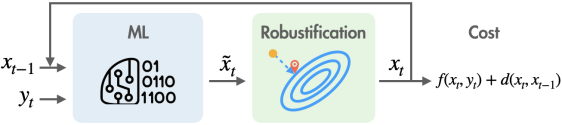
Figure 1: ERL. Given each online input, we first run forward inference to obtain the ML action, and then project it into an expert-robusitfied action space as the actual action.

The ERL inference process is shown in Fig. 1 and described in Algorithm 1. At each step $t$, we run the ML model to produce an action $\tilde{x}_{t}$, get the expert’s action $x_{t}^{\pi}$, and then project $\tilde{x}_{t}$ into a robustified action space by solving Eqn. (2). Note that the expert online algorithm takes context $y_{t}$ as its input and outputs its action $x_{t}^{\pi}$ independently following its own trajectory without being affected by the ML action. Next, we formally provide the robustness analysis for ERL.

Algorithm 1 Expert-Robustified Learning (ERL)

0:  $\lambda\geq 1$, $B\geq 0$, initial $x_{0}$, trained ML model (Section IV-C), and expert online algorithm $\pi$

1:  for $t=1,\cdots,T$

2:   Receive the context $y_{t}$

3:   Expert chooses $x_{t}^{\pi}$ and ML chooses $\tilde{x}_{t}\leftarrow h(x_{t-1},y_{t})$

4:   $x_{t}\leftarrow\text{proj}(\tilde{x}_{t},x_{t}^{\pi},\text{cost}(x_{1:t-1}),\text{cost}(x_{1:t}^{\pi}))$ based on Eqn. (2)  //Robustification

Theorem IV.1

Let $\pi$ be any expert online algorithm for the problem in Eqn. (1). For any $\lambda\geq 1$ and $B\geq 0$, ERL is $\lambda$-competitive against $\pi$ subject to an additive factor of $B$, i.e., $\mathrm{cost}(\texttt{ERL},\bm{s})\leq\lambda\cdot\mathrm{cost}(\pi,\bm{s})+B$ for any input $\bm{s}=(x_{0},\bm{y})$.

Theorem IV.1 is proved in Appendix -B and demonstrates the power of ERL by showing that it can achieve any competitive ratio of $\lambda\geq 1$ with respect to any expert algorithm $\pi$ for $B\geq 0$. Here, given any $B\geq 0$, the hyperparameter $\lambda\geq 1$ can be viewed as the trust parameter: the higher $\lambda$, the more we trust the ML action $\tilde{x}_{t}$, thus potentially achieving a lower average cost at the expense of a higher competitive ratio. The additive factor $B\geq 0$ represents a slackness, and $B=0$ reduces to the strict competitive ratio definition. If we set $\lambda=1$ and $B$ sublinear in $T$, ERL is guaranteed to be asymptotically no worse than the expert $\pi$ even in the worst case as $T\to\infty$.

Competitive ratio of ERL against OPT. One may also desire a bounded competitive ratio against the optimal offline algorithm OPT. To this end, we consider a state-of-the-art expert online algorithm, called Robust, which minimizes the hitting cost at each step without considering the memory cost. This simple online algorithm surprisingly achieves a good competitive ratio of $\max\left(\frac{2}{\alpha},1\right)$ against OPT for $\alpha$-polyhedral hitting cost functions [42]. By applying Theorem IV.1, we have the following corollary.

Corollary IV.1

Consider Robust as the algorithm $\pi$ that chooses $x_{t}=\arg\min_{x\in\mathcal{X}}f(x,y_{t})$ for any $t$. Assume that the hitting cost functions $f(x,y_{t})$ are $\alpha$-polyhedral. For any $\lambda\geq 1$ and $B\geq 0$, ERL is $\lambda\cdot\max\left(\frac{2}{\alpha},1\right)$-competitive against OPT subject to an additive factor of $B$, i.e., $\mathrm{cost}(\texttt{ERL},\bm{s})\leq\lambda\cdot\max\left(\frac{2}{\alpha},1\right)\cdot\mathrm{cost}(\texttt{OPT},\bm{s})+B$ for any input $\bm{s}=(x_{0},\bm{y})$.

IV-C End-to-end Training

In conventional ML-augmented algorithms [12, 6], the ML model is trained to produce good actions on its own, without being aware of the downstream modification (i.e., expert robustification in ERL). While the designed algorithm may sometimes retain good ML actions (i.e., termed as consistency [6]), this still creates a mismatch between training and testing processes — the training process yields good pre-robustification ML actions, but it is post-robustification actions that are actually being used for testing [23, 3, 29, 38]. Thus, to improve the average performance of ERL, we need to explicitly consider the projection step for ML model training.

End-to-end training is highly non-trivial, since the projection step itself is an optimization problem in Eqn. (2) and hence an implicit layer. Additionally, unlike typical differentiable optimizers [1, 4, 38], we need to derive gradients to perform backpropagation through time due to the recurrent nature of our online optimization problem. Let $w$ be the weight for each base ML model $\tilde{x}_{t}=h_{w}(x_{t-1},y_{t})$ in the RNN as illustrated in Fig. 1. We need to derive the gradient of $\text{cost}(x_{1:T})$ with respect to $w$ as follows:

$$\nabla_{w}\text{cost}(x_{1:T})=\sum_{t=1}^{T}\nabla_{w}\big{(}f(x_{t},y_{t})+d(x_{t},x_{t-1})\big{)},$$ (3)

where $x_{t}=\text{proj}(\tilde{x}_{t},x_{t}^{\pi},\text{cost}(x_{1:t-1}),\text{cost}(x_{1:t}^{\pi}))$ is the post-robustification action at step $t=1,\cdots,T$. Thus, the total gradient can be calculated by summing up all the gradients over $T$ steps. By applying the chain rule for step $t$, we have $\nabla_{w}\big{(}f(x_{t},y_{t})+d(x_{t},x_{t-1})\big{)}=\nabla_{x_{t}}\big{(}f(x_{t},y_{t})+d(x_{t},x_{t-1})\big{)}\nabla_{w}{x_{t}}+\nabla_{x_{t-1}}d(x_{t},x_{t-1})\cdot\nabla_{w}{x_{t-1}}$, where $\nabla_{w}{x_{t}}=\left(\nabla_{\tilde{x}_{t}}x_{t}\nabla_{w}\tilde{x}_{t}+\nabla_{\text{cost}(x_{1:t-1})}x_{t}\nabla_{w}\text{cost}(x_{1:t-1})\right)$. The gradients $\nabla_{x_{t}}\big{(}f(x_{t},y_{t})+d(x_{t},x_{t-1})\big{)}$ and $\nabla_{x_{t-1}}d(x_{t},x_{t-1})$ can be obtained given explicit forms of $f$ and $d$, $\nabla_{w}\tilde{x}_{t}$ can be calculated easily through the backpropagation within the ML model (e.g., a neural network), and $\nabla_{w}\text{cost}(x_{1:t-1})$ is calculated recursively back to $t=1$. Thus, the key is to derive the gradients of the projection operator $x_{t}=\text{proj}(\tilde{x}_{t},x_{t}^{\pi},\text{cost}(x_{1:t-1}),\text{cost}(x_{1:t}^{\pi}))$ with respect to the ML action $\tilde{x}_{t}$ and $\text{cost}(x_{1:t-1})$. We provide the result based on KKT conditions [8] in the following proposition.

Proposition IV.2 (Gradient by KKT conditions)

Assume that $x_{t}$ and $\mu$ are the primal and dual solutions to Eqn. (2), respectively. Let $\Delta_{11}=I+\mu\Big{(}\nabla_{x_{t},x_{t}}\big{(}f(x_{t},y_{t})+d(x_{t},x_{t-1})\big{)}+\nabla_{x_{t},x_{t}}d(x_{t},x_{t}^{\pi})\Big{)}$, $\Delta_{12}=\nabla_{x_{t}}\big{(}f(x_{t},y_{t})+d(x_{t},x_{t-1})\big{)}+\nabla_{x_{t}}d(x_{t},x_{t}^{\pi})$, $\Delta_{21}=\mu\Big{(}\nabla_{x_{t}}\big{(}f(x_{t},y_{t})+d(x_{t},x_{t-1})\big{)}+\nabla_{x_{t}}d(x_{t},x_{t}^{\pi})\Big{)}^{\top}$, $\Delta_{22}=f(x_{t},y_{t})+d(x_{t},x_{t-1})+d(x_{t},x_{t}^{\pi})+\text{cost}(x_{1:t-1})-\left[\lambda\text{cost}(x_{1:t}^{\pi})+B\right]$. The gradients of the projection operation $x_{t}=\text{proj}(\tilde{x}_{t},x_{t}^{\pi},\text{cost}(x_{1:t-1}),\text{cost}(x_{1:t}^{\pi}))$ with respect to $\tilde{x}_{t}$ and $\text{cost}(x_{1:t-1})$ are

$$\nabla_{\tilde{x}_{t}}x_{t}=\Delta_{11}^{-1}[I+\Delta_{12}Sc(\Delta,\Delta_{11})^{-1}\Delta_{21}\Delta_{11}^{-1}],$$

$$\nabla_{\text{cost}(x_{1:t-1})}x_{t}=\Delta_{11}^{-1}\Delta_{12}Sc(\Delta,\Delta_{11})^{-1}\mu,$$

where $Sc(\Delta,\Delta_{11})=\Delta_{22}-\Delta_{21}\Delta^{-1}_{11}\Delta_{12}$ is the Schur-complement of $\Delta_{11}$ in the blocked matrix $\Delta=\big{[}[\Delta_{11},\Delta_{12}],[\Delta_{21},\Delta_{22}]\big{]}$.

We remark that if the Schur-complement $Sc(\Delta,\Delta_{11})$ is not full-rank (e.g., ML action $\tilde{x}_{t}$ lies in the boundary of the action space in Eqn. (2)) or the hitting cost function $f$ or memory cost $d$ is not differentiable for certain $x_{t}$, we can still approximate the gradients based on Proposition IV.2 for backpropagation. Concretely, the pseudo-inverse of $Sc(\Delta,\Delta_{11})$ can be used if $Sc(\Delta,\Delta_{11})$ is not full-rank; if $f$ or $d$ is not differentiable at $x_{t}$, we can use its its subgradient as a substitute. This is also a common technique to handle non-differentiable points when training ML models, especially neural networks [18]. For example, we often use $0$ as a subgradient for $ReLu(x)$ at $x=0$. Importantly, Proposition IV.2 provides a practically convenient way to perform backpropagation.

Training. As in typical ML-based approaches for online optimization [3, 21, 2, 14], we train the ML model based on pre-collected historical problem instances by using the gradients in Proposition IV.2 and explicitly considering the projection process. Additionally, we can also update the ML model online by collecting batches of new problem instances during online inference. The training process can be supervised by using the total cost $\sum_{i}\mathrm{cost}_{i}(x_{1:T})$ as the loss where $i$ is the index for training problem instances.

V Extension to Multi-Step Memory Cost

Motivated by smoothness in higher-order dynamics, we now turn to a more general case where the memory cost can span multiple steps: $d(x_{t},x_{t-q:t-1})=\|x_{t}-\sum_{i=1}^{q}C_{i}x_{t-i}\|$, where $q\geq 1$ is the memory length and $C_{i}\in\mathbb{R}^{d\times d}$ is problem-specific. For example, let us consider a robot motion planning problem where $x_{t}$ represents the position at time $t$ and acceleration smoothness is highly desired. In this case, the memory cost can be written as $d(x_{t},x_{t-2:t-1})=\|\left(x_{t}-x_{t-1}\right)-\left(x_{t-1}-x_{t-2}\right)\|=\|x_{t}-2x_{t-1}+x_{t-2}\|$, for which we can set $C_{1}=-2\cdot I$, $C_{2}=I$ and $q=2$ where $I$ is the identity matrix in $\mathbb{R}^{d\times d}$. Note that the expert algorithm in [35] uses the same form of multi-step memory structure, but considers a squared memory cost along with other strong assumptions (e.g., strongly convex hitting costs) that require entirely different techniques [42]. To our knowledge, our work is the first to consider multi-step memory costs in metric space.

Expert robustification. Given multi-step memory costs, the input to our ML model includes $y_{t}$ and $x_{t-q:t-1}$ and outputs $\tilde{x}_{t}$, which is then robustified by solving the following:

$$\begin{split}\begin{gathered}x_{t}=\arg\min_{x\in\mathcal{X}}\frac{1}{2}\|x-\tilde{x}_{t}\|^{2}\\ s.t.\;\;\;\;\;\mathrm{cost}({x}_{1:t-1})+f(x,y_{t})+d(x,x_{t-q:t-1})\\ +G(x,{x}_{t-q:t-1},{x}_{t-q:t}^{\pi})\leq\lambda\mathrm{cost}({x}_{1:t}^{\pi})+B,\end{gathered}\end{split}$$ (4)

where the reservation cost $G(x,{x}_{t-q:t-1},{x}_{t-q:t}^{\pi})$ is given by

$$\begin{split}&G\left(x,{x}_{t-q:t-1},{x}_{t-q:t}^{\pi}\right)\\ =&\sum_{k=1}^{\min(q,T-t)}{\left\|C_{k}x+\sum_{i=1}^{q-k}C_{k+i}x_{t-i}-\sum_{i=0}^{q-k}C_{k+i}x_{t-i}^{\pi}\right\|}.\end{split}$$ (5)

The key insight for Eqn. (5) is that we need to account for the potentially higher memory costs incurred by ERL compared to the expert algorithm $\pi$ over up to future $q$ steps. By holding the reservation cost for the cumulative cost at each step, we can ensure that ERL can always roll back to the expert’s actions in the future without violating the robustness requirement. The ERL inference process still follows Algorithm 1, except for that the projection step for expert robustification in Line 5 is based on Eqn. (4).

Competitive ratio of Robust. Robust has a bounded competitive ratio in the single-step memory setting [42], but it is unclear in the multi-step setting. Here, we prove that Robust is also competitive in the multi-step memory case. The proof is in Appendix -A.

Theorem V.1

Assume that $f(\cdot,y_{t}):\mathcal{X}\mapsto\mathbb{R}$ is $\alpha$-polyhedral and that the memory cost is given by $d(x_{t},x_{t-q:t-1})=\|x_{t}-\sum_{i=1}^{q}C_{i}x_{t-i}\|$ for $t=1,\cdots,T$, where $C_{i}\in\mathbb{R}^{d\times d}$ and $\sum_{i=1}^{q}\|C_{i}\|=\beta$ with $\|C_{i}\|$ being the matrix norm induced by the $l_{p}$ vector norm. The Robust algorithm that chooses $x_{t}=\arg\min_{x\in\mathcal{X}}f(x,y_{t})$ for any $t=1,\cdots,T$ is strictly $\max\left(\frac{\beta+1}{\alpha},1\right)$-competitive against OPT, i.e., $\mathrm{cost}(\texttt{Robust},\bm{s})\leq\max\left(\frac{\beta+1}{\alpha},1\right)\cdot\mathrm{cost}(\texttt{OPT},\bm{s})$ for any input $\bm{s}=(x_{0},\bm{y})$.

Competitive ratio of ERL. In the multi-step memory case, Theorem IV.1 still holds. That is, for any $\lambda\geq 1$ and $B\geq 0$, ERL is still $\lambda$-competitive against any expert online algorithm $\pi$ subject to an additive factor $B$. Also, by combining this result with Theorem V.1, we obtain the following corollary (proof in Appendix -B).

Corollary V.1

Let the expert $\pi$ be Robust that chooses $x_{t}=\arg\min_{x\in\mathcal{X}}f(x,y_{t})$ for any $t=1,\cdots,T$. Under the same assumptions as in Theorem V.1, for any $\lambda\geq 1$ and $B\geq 0$, ERL is $\lambda\max\left(\frac{\beta+1}{\alpha},1\right)$-competitive against OPT subject to an additive factor of $B$ where $\beta=\sum_{i=1}^{q}\|C_{i}\|$, i.e., $\mathrm{cost}(\texttt{ERL},\bm{s})\leq\lambda\max\left(\frac{\beta+1}{\alpha},1\right)\cdot\mathrm{cost}(\texttt{OPT},\bm{s})+B$ for any input $\bm{s}=(x_{0},\bm{y})$.

Finally, for end-to-end training, the gradients of projection in Eqn. (4) with respect to $\tilde{x}_{t}$ and $\text{cost}(x_{1:t-1})$ can be derived and the ML model can be trained following the steps in Section IV-C. Hence, we omit them for brevity.

VI Experimental Results

To empirically validate ERL, we consider the dynamic energy scheduling application in the presence of uncertain renewables. Specifically, renewable energy such as wind and solar energy is being massively incorporated into the power grid for sustainability. But, their availability is highly intermittent subject to a variety of factors such as weather conditions and equipment efficiency. On the other hand, balancing the power demand and generation is crucial to ensure grid stability — a mismatch requires rapid offsetting using alternative and potentially more expensive energy sources. Thus, a challenging problem faced by grid operators is how to dynamically schedule energy production to meet net demands based on real-time renewable availability. A mismatch between the production $x_{t}$ and net demand $y_{t}$ needs offsetting using expensive energy sources/storage and hence causes a hitting cost $f(x_{t},y_{t})=\alpha\|x_{t}-y_{t}\|$, and varying the production level over time incurs a memory cost $d(x_{t},x_{t-1})=\|x_{t}-x_{t-1}\|$ (due to generator ramp-up/-down costs). Thus, this is a typical online optimization problem with memory cost [25, 23, 42].

VI-A Dataset

We consider intermittent renewable energy generated using trace data and empirical equations. Specifically, for wind power, the amount of energy generated at step $t$ is modeled based on [33] as $P_{\mathrm{wind},t}=\frac{1}{2}\kappa_{\mathrm{wind}}\varrho A_{\mathrm{swept}}V_{\mathrm{wind},t}^{3}$.

The sympols are explained as follows: $\kappa_{\mathrm{wind}}$ is the conversion efficiency (%) of wind energy, $\varrho$ is the air density ($kg/m^{3}$), $A_{\mathrm{swept}}$ is the swept area of the turbine ($m^{2}$), and $V_{\mathrm{wind},t}$ is the wind speed ($kW/m^{2}$) at time step $t$. The amount of solar energy generated at step $t$ is given based on [37] as $P_{\mathrm{solar},t}=\frac{1}{2}\kappa_{\mathrm{solar}}A_{\mathrm{array}}I_{\mathrm{rad},t}(1-0.05*(\mathrm{Temp}_{t}-25))$. The symbols are explained as follows: $\kappa_{\mathrm{solar}}$ is the conversion efficiency (%) of the solar panel, $A_{\mathrm{array}}$ is the array area ($m^{2}$), and $I_{\mathrm{rad},t}$ is the solar radiation ($kW/m^{2}$), and $\mathrm{Temp}_{t}$ is the temperature (^∘C) at step $t$. Thus, at time step $t$, the total energy generated by the renewables $P_{\mathrm{r},t}=P_{\mathrm{wind},t}+P_{\mathrm{solar},t}$. Suppose at time step $t$, the net energy demand is $y_{t}=\max(P_{\mathrm{s},t}-P_{\mathrm{r},t},0)$ , where $P_{\mathrm{s},t}$ is the demand before renewable integration. The amount of energy generation is the agent’s online action $x_{t}$. We model the hitting cost as the scaled $l_{2}$-norm of the difference between the action $x_{t}$ and the context $y_{t}$, i.e. $f(x_{t},y_{t})=\alpha\|x_{t}-y_{t}\|$. Additionally, we model the switching cost by the $l_{2}$-norm of the difference between two consecutive actions, i.e. $c(x_{t},x_{t-1})=\|x_{t}-x_{t-1}\|$. The hitting cost parameter is set as $\alpha=0.2$. The parameters for wind energy are set as $\kappa_{\mathrm{wind}}=30\%$, $\varrho=1.23kg/m^{3}$, $A_{\mathrm{swept}}=500,000m^{2}$. The parameters of solar energy are set as $\kappa_{\mathrm{wind}}=10\%$, $A_{\mathrm{array}}=10,000m^{2}$. The other parameters, such as wind speed, solar radiation and temperature data, are all collected from the National Solar Radiation Database [34], which contains detailed hourly data for the year of 2015.

To generate datasets for training and testing, we use a sliding window to generate multiple sequences of hourly data, with each sequence length being 25 (i.e., 24 action steps plus 1 initial step). For each sequence of 25 consecutive hourly data, we can calculate the contextual information for each step/hour. We define the energy generation of the first hour as the initial action $x_{0}$. The problem can be formulated as: $\min_{x_{1},\cdots x_{T}}\sum_{t=1}^{T}\alpha\|x_{t}-y_{t}\|+\|x_{t}-x_{t-1}\|$. We use the CVXPY Library to find the optimal offline solution.

VI-B Experimental Setup

We use a RNN with 2 hidden layers, each with 8 neurons. To train this model, we use the data from the first two months (January–February) of 2015, which contains 1440 hourly weather data samples in total. Specifically, we generate 1416 data sequences using a sliding window. We train the RNN model for 140 epochs with batch size of 50. The model is implemented in PyTorch Library and the training process usually takes around 3 minutes on a 2020 MacBook Air with 8GB memory and a M1 chipset. In ERL, we set the slackness parameter $B=0$ to follow the strict definition of competitive ratio. By default, we train ERL with $\lambda=1.4$.

To evaluate the performance of different algorithms, we divide the remaining 10 months of 2015 into five segments, each with two months. There are three different cases: when ML empirically works better than Robust in terms of both average and worst-case performance; ML is better than Robust on average but worse in the worst case; and ML is worse than Robust both on average and in the worst case. The first case occurs for the testing segment of March–April, because the data in both training and testing datasets well consistent due to their similar weather patterns. Next, we focus on the other two cases, which are more interesting and typical since data distributional shifts between training and testing datasets are very common in practice. This is also consistent with our main contribution — robustifying ML-based optimizers.

While we can also re-train/update the ML models (in ERL, ML, and ERL-NT) based on online collected data, the existing ML-based optimizers are typically pre-trained offline [2, 15]. Thus, we keep the ML model unchanged when testing its performance, in order to highlight the role of our expert robustification step in ERL— regardless of the testing distributions, ERL offers a provable worst-case competitive ratio guarantee against the expert.

VI-C Baselines

We compare ERL with the following baselines. Optimal offline (OPT): OPT has all the context information to optimally solve Eqn. (1); Robust expert (Robust): Robust is the state-of-the-art expert that chooses $x_{t}=\arg\min_{x\in\mathcal{X}}f(x,y_{t})$ for $t=1,\cdots,T$ with guaranteed competitive ratios [42]; Simple greedy (Greedy): Greedy greedily minimizes the total hitting cost and memory cost at each step; Pure ML-based optimizer (ML): ML uses the same recurrent neural network as ERL but does not use expert robustification for training or inference; Dynamic switching (Switch): Switch dynamically switches between Robust and ML based on a threshold hyperparameter [6]; ERL-NoTraining (ERL-NT): ERL-NT uses Algorithm 1 for inference but the ML model is trained as a standalone optimizer without end-to-end training.

Although Greedy may empirically perform better than Robust, it does not have a provably-bounded competitive ratio whereas Robust has one (see [42] for the single-step memory case and our Theorem V.1 for the multi-step memory case). Thus, we use Robust as our expert in ERL.

VI-D Results

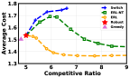
(a) September-December testing

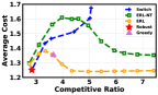
(b) May-August testing

Figure 2: Normalized average cost vs. empirical competitive ratio. ML is off the charts: (left): average cost 1.45 and competitive ratio 50+; (right): average cost 1.367 and competitive ratio 11.167.

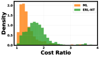
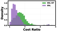
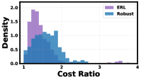
Figure 3: Cost ratio probability distribution for September-December testing. The density values are obtained by dividing the number of testing instances within each bin by the total number of instances and the bin width. We use $\lambda=1.4$ for testing ERL-NT and ERL. The horizontal axis is limit to $4$ for better visualization, and cost ratios larger than 4 are off the charts.

September-December testing. We obtain the empirical results of average cost vs. competitive ratio in Fig. 2. All the average costs are normalized with respect to the average cost of OPT. ML achieves a lower average cost than Robust, but its empirical competitive ratio is way larger due to the common drawback of ML-based optimizers — lack of performance robustness. Specifically, the training and testing distributions are rarely identical in practice, which can lead to an extremely bad competitive ratio for ML. While Greedy empirically performs better than Robust in this setting, it does not have any competitive ratio guarantees. We see that Switch performs badly compared to Robust, because it imposes a hard switch based on a pre-set threshold regardless of the actual performance of Robust or ML. Compared to ML, ERL-NT can have a much lower competitive ratio due to expert robustification, but the average cost also increases dramatically and can be even higher than Robust (because the ML model training in ERL-NT is not aware of the robustification step). On the other hand, ERL achieves a guaranteed competitive ratio and a much lower average cost than ERL-NT. This highlights the benefits of training the ML model in ERL by explicitly considering the downstream expert robustification process. Interestingly, we also observe that by properly setting the hyperparameter $\lambda$ (around $1.4\sim 1.8$ in our case), ERL can have an even lower average cost than ML. This is because for those hard problem instances that ML cannot solve well, ERL has Robust as its guidance to provide reasonably good solutions.

Cost ratio distribution. To provide further insights, we also show in Fig. 3 the detailed comparison between different algorithm pairs in terms of the cost ratio distribution density. By looking at Robust vs. ML in Fig. 3, we can see that ML has low cost ratios in more cases than Robust, although it has a long tail (not shown in the figure due to the axis limit). This explains that ML can have good average performance than the expert algorithm Robust, when the training-testing distributions are not very different. Nonetheless, ML still suffers from the lack of robustness, while Robust does not. Comparing ML with ERL-NT in Fig. 3, we can see that expert robustification can shift the cost ratios rightwards (i.e., increasing the average cost), but ERL-NT has guaranteed robustness. Next, we observe from Fig. 3 that the cost ratios of ERL are shifted leftwards compared to ERL-NT, demonstrating the importance of training ERL with explicit consideration of the expert robustification process. Fig. 3 shows that ERL has many smaller cost ratios than Robust. Again, this shows the importance of considering expert robustficniation during the training process.

	ERL-NT		ERL ($\lambda$ = 1.4)		ERL ($\lambda$ = 1.2)		Switch		Robust		Greedy
$\lambda$ for Testing	Avg	CR	Avg	CR	Avg	CR	Avg	CR	Avg	CR	Avg	CR
$\lambda$ = 1.4	1.6977	6.0912	1.3903	6.0910	1.4343	6.0910	1.7454	6.4130	1.5336	5.000	1.5030	4.800
$\lambda$ = 1.2	1.6457	5.5457	1.4832	5.5456	1.4587	5.5456	1.7454	6.4130	1.5336	5.000	1.5030	4.800

TABLE I: September-December testing. “Avg” and “CR” represent the empirical average cost and competitive ratio (normalized w.r.t. OPT), respectively. Bold texts mean the best AVG performance. ERL ($\lambda=x$) means we train ERL with $\lambda=x$.

Impacts of $\lambda.$ While both ERL and ERL-NT can guarantee robustness due to the expert robustification step during inference, the ML model in ERL is trained with explicit consideration of the expert whereas ERL-NT simply trains the ML model as a standalone optimizer. Thus, ERL can further improve the average performance compared to ERL-NT. To further highlight the necessity of being aware of the expert robustification step in the training of ERL, we show the results for different algorithms in Table I. By training ERL using the same $\lambda$ as testing it, we can obtain both the best average cost and the best competitive ratio empirically. In particular, the difference in terms of the average performance is more prominent when $\lambda=1.4$ than when $\lambda=1.2$. This can be explained by noting that with a larger $\lambda\geq 1$, the expert plays a less significant role by placing less emphasis on robustness and providing the ML model with more freedom. Then, when $\lambda=1.4$, the average performance is better than when $\lambda=1.2$, although its guaranteed competitive ratio is higher (which is also empirically verified in Table I). For reference, we also show the performance of other algorithms that are not affected by $\lambda\geq 1$.

May-August testing. Next, we turn to a more challenging case in which ML is outperformed by Robust both on average and in the worst case (May–August, due to the different weather patterns and hence large training-testing distributional shifts). This is not uncommon in practice, since ML models can have arbitrarily bad performances due to the lack of robustness. We show the results in Fig. 2(b). All the average values are normalized with respect to the average cost of OPT.

Again, ML is off the charts, with its competitive ratio as 11.167 and average cost as 1.367 (both normalized with respect to OPT). Like in the previous case, Switch is not as good as Robust, since it utilizes a hard switching between Robust and ML whenever a pre-defined threshold is reached without looking at the actual performance of Robust or ML. Due to the lack of robustness guarantees, Greedy is also worse than Robust in this setting. By varying $\lambda\geq 1$, we see that ERL-NT can have very large average costs (even larger than ML), although its competitive ratio is still guaranteed to be $\lambda$-competitive against the expert Robust. On the other hand, ERL, which is trained with $\lambda=1.4$ and tested with different $\lambda\geq 1$ has a much lower average cost than ERL-NT, while also being able to guarantee competitive ratios. This shows the importance of being aware of expert robustification during the training stage. Moreover, ERL has a lower average cost than ML: even in the presence of large training-testing distributional discrepancies, the expert can help correct many of the bad pre-robustification actions, thus significantly improving the average performance of ERL over ML. Interestingly, the average performance of ERL is not monotonic in the parameter of $\lambda\geq 1$ used for testing. This is partly because $\lambda$ is different for training and testing, and partly because the large training-testing distributional discrepancies result in irregular average performance for the ML model used by ERL. By $\lambda=1$, we essentially have no trust on the ML model in ERL, and hence ERL will follow the expert Robust at each step.

Summary. Our experiments highlight the key point that ERL guarantees worst-case robustness in terms of the competitive ratio by utilizing expert robustification, while exploiting the power of ML to improve the average performance. Naturally, when training-testing distributions are reasonably similar, we expect the average performance of ERL (and other ML-based optimizers like ML) to be better than that of Robust. But, even when the pure ML performs arbitrarily badly, ERL can still offer a good average cost performance due to the introduction of expert robustification. Last but not least, with explicit awareness of the expert robustification process, ERL has a much better average performance than otherwise (i.e., ERL-NT).

VII Conclusion

In this paper, we propose ERL, a novel expert-robustified learning approach to solve online optimization with memory costs. For guaranteed robustness, ERL introduces a projection operator that robustifies ML actions by utilizing an expert online algorithm; for good average performance, ERL trains the ML optimizer based on a recurrent architecture by explicitly considering downstream expert robustification process. We prove that, for any $\lambda\geq 1$, ERL can achieve $\lambda$-competitive against the expert algorithm for any problem inputs. We also extend our analysis to a novel setting of multi-step memory costs. Finally, we run experiments for an energy scheduling application to validate ERL, showing that ERL can offer the best tradeoff in terms of the average and worst performance.

References

- [1] Akshay Agrawal, Brandon Amos, Shane Barratt, Stephen Boyd, Steven Diamond, and J. Zico Kolter. Differentiable convex optimization layers. In H. Wallach, H. Larochelle, A. Beygelzimer, F. d'Alché-Buc, E. Fox, and R. Garnett, editors, Advances in Neural Information Processing Systems, volume 32. Curran Associates, Inc., 2019.
- [2] Mohammad Ali Alomrani, Reza Moravej, and Elias B. Khalil. Deep policies for online bipartite matching: A reinforcement learning approach. CoRR, abs/2109.10380, 2021.
- [3] Brandon Amos. Tutorial on amortized optimization for learning to optimize over continuous domains. CoRR, abs/2202.00665, 2022.
- [4] Brandon Amos, Ivan Jimenez, Jacob Sacks, Byron Boots, and J. Zico Kolter. Differentiable MPC for end-to-end planning and control. In S. Bengio, H. Wallach, H. Larochelle, K. Grauman, N. Cesa-Bianchi, and R. Garnett, editors, Advances in Neural Information Processing Systems, volume 31. Curran Associates, Inc., 2018.
- [5] Keerti Anand, Rong Ge, Amit Kumar, and Debmalya Panigrahi. A regression approach to learning-augmented online algorithms. In A. Beygelzimer, Y. Dauphin, P. Liang, and J. Wortman Vaughan, editors, Advances in Neural Information Processing Systems, 2021.
- [6] Antonios Antoniadis, Christian Coester, Marek Elias, Adam Polak, and Bertrand Simon. Online metric algorithms with untrusted predictions. In ICML, 2020.
- [7] Joan Boyar, Lene M. Favrholdt, Christian Kudahl, Kim S. Larsen, and Jesper W. Mikkelsen. Online algorithms with advice: A survey. SIGACT News, 47(3):93–129, August 2016.
- [8] S. Boyd and L. Vandenberghe. Convex Optimization. Cambridge University Press, 2004.
- [9] Niangjun Chen, Joshua Comden, Zhenhua Liu, Anshul Gandhi, and Adam Wierman. Using predictions in online optimization: Looking forward with an eye on the past. SIGMETRICS Perform. Eval. Rev., 44(1):193–206, June 2016.
- [10] Niangjun Chen, Gautam Goel, and Adam Wierman. Smoothed online convex optimization in high dimensions via online balanced descent. In COLT, 2018.
- [11] Jakub Chłędowski, Adam Polak, Bartosz Szabucki, and Konrad Tomasz Żołna. Robust learning-augmented caching: An experimental study. In ICML, 2021.
- [12] Nicolas Christianson, Tinashe Handina, and Adam Wierman. Chasing convex bodies and functions with black-box advice. In COLT, 2022.
- [13] Joshua Comden, Sijie Yao, Niangjun Chen, Haipeng Xing, and Zhenhua Liu. Online optimization in cloud resource provisioning: Predictions, regrets, and algorithms. Proc. ACM Meas. Anal. Comput. Syst., 3(1), March 2019.
- [14] Bingqian Du, Zhiyi Huang, and Chuan Wu. Adversarial deep learning for online resource allocation. ACM Trans. Model. Perform. Eval. Comput. Syst., 6(4), feb 2022.
- [15] Bingqian Du, Chuan Wu, and Zhiyi Huang. Learning resource allocation and pricing for cloud profit maximization. In Proceedings of the Thirty-Third AAAI Conference on Artificial Intelligence and Thirty-First Innovative Applications of Artificial Intelligence Conference and Ninth AAAI Symposium on Educational Advances in Artificial Intelligence, AAAI’19/IAAI’19/EAAI’19. AAAI Press, 2019.
- [16] Elbert Du, Franklyn Wang, and Michael Mitzenmacher. Putting the “learning" into learning-augmented algorithms for frequency estimation. In Marina Meila and Tong Zhang, editors, Proceedings of the 38th International Conference on Machine Learning, volume 139 of Proceedings of Machine Learning Research, pages 2860–2869. PMLR, 18–24 Jul 2021.
- [17] Gautam Goel, Yiheng Lin, Haoyuan Sun, and Adam Wierman. Beyond online balanced descent: An optimal algorithm for smoothed online optimization. In NeurIPS, volume 32, 2019.
- [18] Ian Goodfellow, Yoshua Bengio, and Aaron Courville. Deep Learning. MIT Press, 2016.
- [19] Elad Hazan. Introduction to online convex optimization. Foundations and Trends® in Optimization, 2(3-4):157–325, 2016.
- [20] Howard Heaton, Xiaohan Chen, Zhangyang Wang, and Wotao Yin. Safeguarded learned convex optimization, 2020.
- [21] Weiwei Kong, Christopher Liaw, Aranyak Mehta, and D. Sivakumar. A new dog learns old tricks: RL finds classic optimization algorithms. In ICLR, 2019.
- [22] Ke Li and Jitendra Malik. Learning to optimize. In ICLR, 2017.
- [23] Pengfei Li, Jianyi Yang, and Shaolei Ren. Expert-calibrated learning for online optimization with switching costs. In SIGMETRICS, 2022.
- [24] Yingying Li, Xin Chen, and Na Li. Online optimal control with linear dynamics and predictions: Algorithms and regret analysis. In NeurIPS, Red Hook, NY, USA, 2019. Curran Associates Inc.
- [25] Yingying Li and Na Li. Leveraging predictions in smoothed online convex optimization via gradient-based algorithms. In NeurIPS, volume 33, 2020.
- [26] Yingying Li, Guannan Qu, and Na Li. Online optimization with predictions and switching costs: Fast algorithms and the fundamental limit. IEEE Transactions on Automatic Control, 2020.
- [27] M. Lin, A. Wierman, L. L. H. Andrew, and E. Thereska. Dynamic right-sizing for power-proportional data centers. In INFOCOM, 2011.
- [28] Yiheng Lin, Gautam Goel, and Adam Wierman. Online optimization with predictions and non-convex losses. Proc. ACM Meas. Anal. Comput. Syst., 4(1), May 2020.
- [29] Heyuan Liu and Paul Grigas. Risk bounds and calibration for a smart predict-then-optimize method. In A. Beygelzimer, Y. Dauphin, P. Liang, and J. Wortman Vaughan, editors, Advances in Neural Information Processing Systems, 2021.
- [30] Yecheng Jason Ma, Dinesh Jayaraman, and Osbert Bastani. Conservative offline distributional reinforcement learning. In A. Beygelzimer, Y. Dauphin, P. Liang, and J. Wortman Vaughan, editors, Advances in Neural Information Processing Systems, 2021.
- [31] Aranyak Mehta. Online matching and ad allocation. Foundations and Trends in Theoretical Computer Science, 8 (4):265–368, 2013.
- [32] Daan Rutten, Nico Christianson, Debankur Mukherjee, and Adam Wierman. Online optimization with untrusted predictions. CoRR, abs/2202.03519, 2022.
- [33] Asis Sarkar and Dhiren Kumar Behera. Wind turbine blade efficiency and power calculation with electrical analogy. International Journal of Scientific and Research Publications, 2(2):1–5, 2012.
- [34] Manajit Sengupta, Yu Xie, Anthony Lopez, Aron Habte, Galen Maclaurin, and James Shelby. The national solar radiation data base (nsrdb). Renewable and Sustainable Energy Reviews, 89:51–60, 2018.
- [35] Guanya Shi, Yiheng Lin, Soon-Jo Chung, Yisong Yue, and Adam Wierman. Online optimization with memory and competitive control. In NeurIPS, volume 33. Curran Associates, Inc., 2020.
- [36] Matthew Staib and Stefanie Jegelka. Distributionally robust optimization and generalization in kernel methods. Advances in Neural Information Processing Systems, 32:9134–9144, 2019.
- [37] Can Wan, Jian Zhao, Yonghua Song, Zhao Xu, Jin Lin, and Zechun Hu. Photovoltaic and solar power forecasting for smart grid energy management. CSEE Journal of Power and Energy Systems, 1(4):38–46, 2015.
- [38] Kai Wang, Sanket Shah, Haipeng Chen, Andrew Perrault, Finale Doshi-Velez, and Milind Tambe. Learning MDPs from features: Predict-then-optimize for sequential decision making by reinforcement learning. In A. Beygelzimer, Y. Dauphin, P. Liang, and J. Wortman Vaughan, editors, Advances in Neural Information Processing Systems, 2021.
- [39] Tsung-Yen Yang, Justinian Rosca, Karthik Narasimhan, and Peter J. Ramadge. Projection-based constrained policy optimization. In International Conference on Learning Representations, 2020.
- [40] Yunchang Yang, Tianhao Wu, Han Zhong, Evrard Garcelon, Matteo Pirotta, Alessandro Lazaric, Liwei Wang, and Simon Shaolei Du. A reduction-based framework for conservative bandits and reinforcement learning. In International Conference on Learning Representations, 2022.
- [41] Jingzhao Zhang, Aditya Krishna Menon, Andreas Veit, Srinadh Bhojanapalli, Sanjiv Kumar, and Suvrit Sra. Coping with label shift via distributionally robust optimisation. In International Conference on Learning Representations, 2021.
- [42] Lijun Zhang, Wei Jiang, Shiyin Lu, and Tianbao Yang. Revisiting smoothed online learning. In A. Beygelzimer, Y. Dauphin, P. Liang, and J. Wortman Vaughan, editors, Advances in Neural Information Processing Systems, 2021.
- [43] Martin Zinkevich. Online convex programming and generalized infinitesimal gradient ascent. In Proceedings of the 20th international conference on machine learning (icml-03), pages 928–936, 2003.