Bidirectional Copy-Paste for Semi-Supervised Medical Image Segmentation

Abstract

In semi-supervised medical image segmentation, there exist empirical mismatch problems between labeled and unlabeled data distribution. The knowledge learned from the labeled data may be largely discarded if treating labeled and unlabeled data separately or in an inconsistent manner. We propose a straightforward method for alleviating the problem $-$ copy-pasting labeled and unlabeled data bidirectionally, in a simple Mean Teacher architecture. The method encourages unlabeled data to learn comprehensive common semantics from the labeled data in both inward and outward directions. More importantly, the consistent learning procedure for labeled and unlabeled data can largely reduce the empirical distribution gap. In detail, we copy-paste a random crop from a labeled image (foreground) onto an unlabeled image (background) and an unlabeled image (foreground) onto a labeled image (background), respectively. The two mixed images are fed into a Student network and supervised by the mixed supervisory signals of pseudo-labels and ground-truth. We reveal that the simple mechanism of copy-pasting bidirectionally between labeled and unlabeled data is good enough and the experiments show solid gains (e.g., over 21% Dice improvement on ACDC dataset with 5% labeled data) compared with other state-of-the-arts on various semi-supervised medical image segmentation datasets. Code is available at https://github.com/DeepMed-Lab-ECNU/BCP.

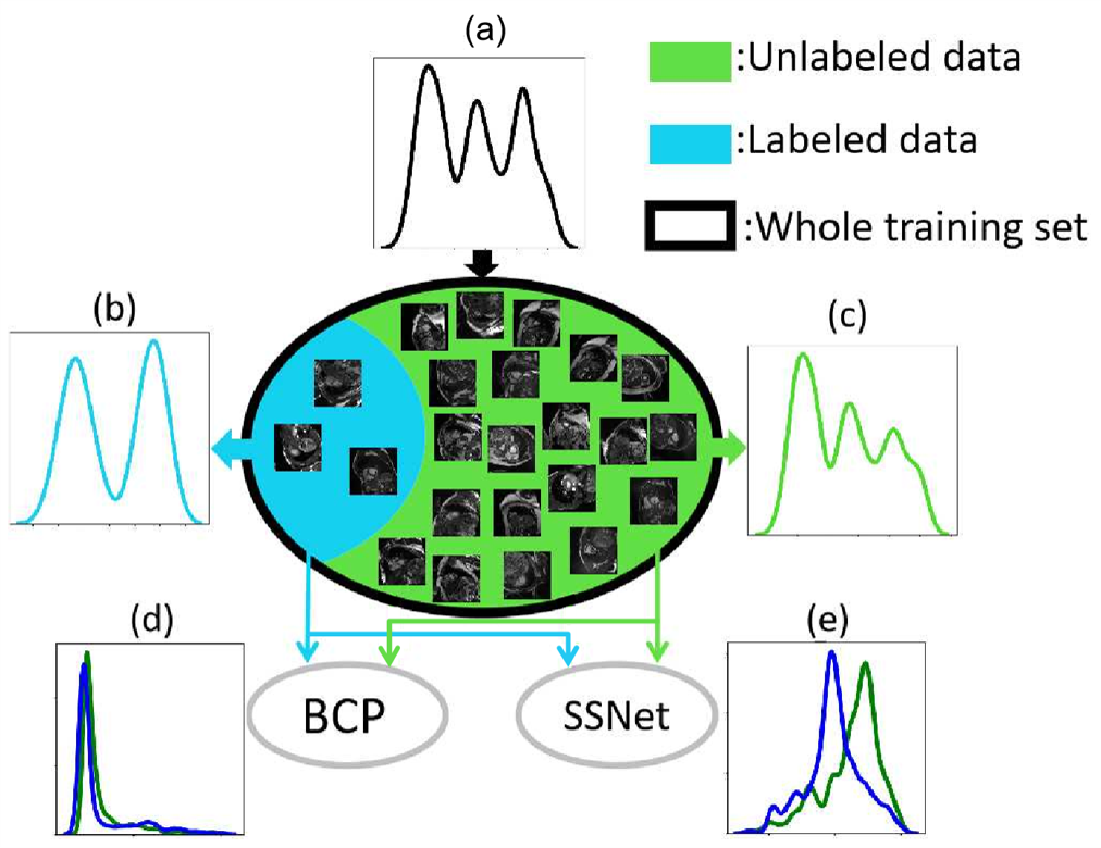
Figure 1: Illustration of the mismatch problem under semi-supervised leaning setting. Assume the training set is drawn from a latent distribution in (a). But the empirical distributions of small amount of labeled data and a large amount of unlabeled data are (b) and (c), respectively. It’s hard to use few labeled data to construct the precise distribution of the whole dataset. (d) By using our BCP, the empirical distributions of labeled and unlabeled features are aligned. (e) But other methods such as SSNet [35] or cross unlabeled data copy-paste cannot address the empirical distribution mismatch issue. All distributions are kernel density estimations of voxels belonging to myocardium class in ACDC [2].

1 Introduction

Segmenting internal structures from medical images such as computed tomography (CT) or magnetic resonance imaging (MRI) is essential for many clinical applications [34]. Various techniques based on supervised learning for medical image segmentation have been proposed [13, 4, 45], which usually requires a large amount of labeled data. But, due to the tedious and expensive manual contouring process when labeling medical images, semi-supervised segmentation attracts more attention in recent years, and has become ubiquitous in the field of medical image analysis.

Generally speaking, in semi-supervised medical image segmentation, the labeled and unlabeled data are drawn from the same distribution, (Fig. 1 (a)). But in real-world scenario, it’s hard to estimate the precise distribution from labeled data because they are few in number. Thus, there always exists empirical distribution mismatch between a large amount of unlabeled and a very small amount of labeled data [30] (Fig. 1(b) and (c)). Semi-supervised segmentation methods always attempt to train labeled and unlabeled data symmetrically, in a consistent manner. E.g., self-training [1, 48] generates pseudo-labels to supervise unlabeled data in a pseudo-supervised manner. Mean Teacher based methods [40] adopt consistency loss to “supervise” unlabeled data with strong augmentations, in analogy with supervising labeled data with ground-truth. DTC [16] proposed a dual-task-consistency framework, applicable to both labeled and unlabeled data. ContrastMask [31] applied dense contrastive learning on both labeled and unlabeled data. But most existing semi-supervised methods used labeled and unlabeled data under separate learning paradigms. Thus, it often leads to the discarding of massive knowledge learned from the labeled data and the empirical distribution mismatch between labeled and unlabeled data (Fig. 1(e)).

CutMix [42] is simple yet strong data processing method, also dubbed as Copy-Paste (CP), which has the potential to encourage unlabeled data to learn common semantics from the labeled data, since pixels in the same map share semantics to be closer [29]. In semi-supervised learning, forcing consistency between weak-strong augmentation pair of unlabeled data is widely used [14, 32, 11, 47], and CP is usually used as a strong augmentation. But existing CP methods only consider CP cross unlabeled data [14, 10, 8], or simply copy crops from labeled data as foreground and paste to another data [9, 6]. They neglect to design a consistent learning strategy for labeled and unlabeled data, which hampers its usage on reducing the distribution gap. Meanwhile, CP tries to enhance the generalization of networks by increasing unlabeled data diversity, but a high performance is hard to achieve since CutMixed image is only supervised by low-precision pseudo-labels. It’s intuitive to use more accurate supervision to help networks segment degraded region cut by CP.

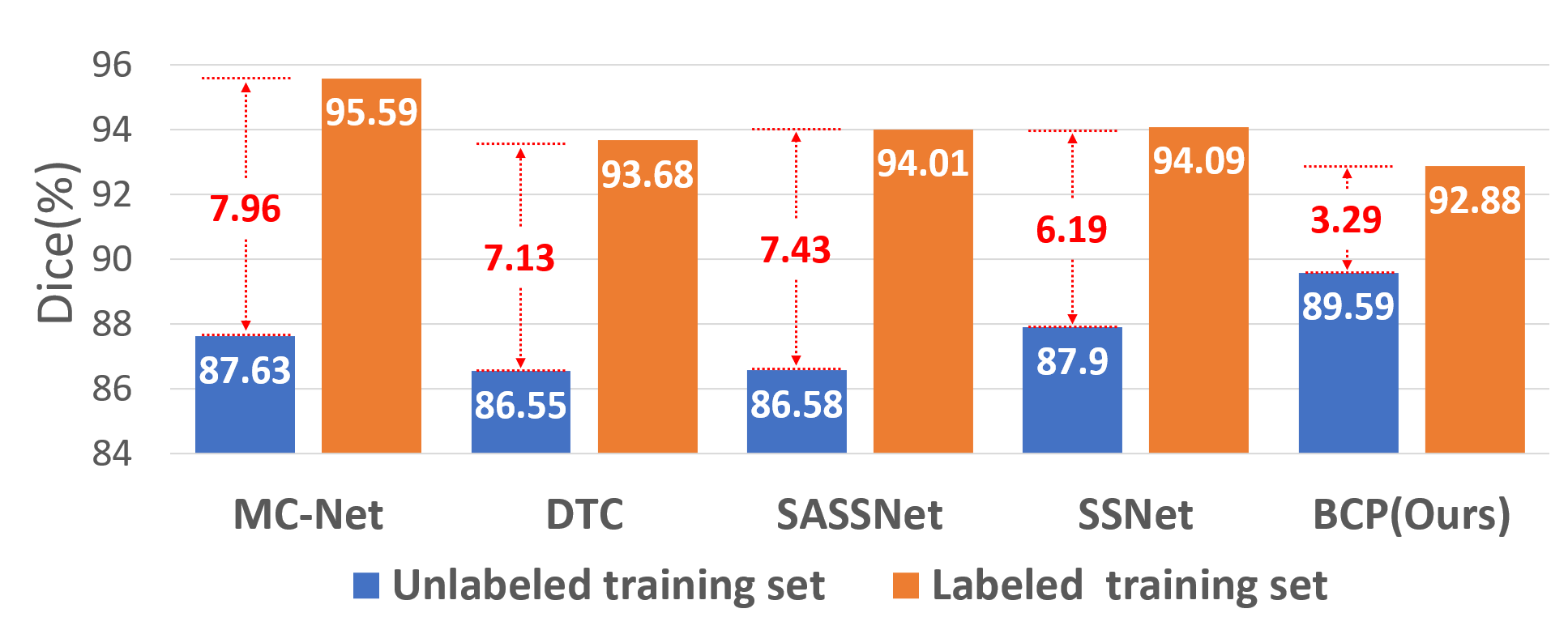
Figure 2: Dice scores for unlabeled and labeled training data of different models on LA dataset [39]. A much smaller performance gap is observed in our method.

To alleviate the empirical mismatch problem between labeled and unlabeled data, a successful design is to encourage unlabeled data to learn comprehensive common semantics from the labeled data, and meanwhile, furthering the distribution alignment via a consistent learning strategy for labeled and unlabeled data. We achieve this by proposing a surprisingly simple yet very effective Bidirectional Copy-Paste (BCP) method, instantiated in the Mean Teacher framework. Concretely, to train the Student network, we augment our inputs by copy-pasting random crops from a labeled image (foreground) onto an unlabeled image (background) and reversely, copy-pasting random crops from an unlabeled image (foreground) onto a labeled image (background). The Student network is supervised by the generated supervisory signal via bidirectional copy-pasting between the pseudo-labels of the unlabeled images from the Teacher network and the label maps of the labeled image. The two mixed images help the network to learn common semantics between the labeled and unlabeled data bidirectionally and symmetrically. We compute the Dice scores for labeled and unlabeled training set from LA dataset [39] based on models trained by state-of-the-arts and our method, as shown in Fig. 2. Previous models which process labeled data and unlabeled data separately present strong performance gap between labeled and unlabeled data. E.g., MC-Net obtains 95.59% Dice for labeled data but only 87.63% for unlabeled data. It means previous models absorb knowledge from ground-truth well, but discard a lot when transferring to unlabeled data. Our method can largely decrease the gap between labeled and unlabeled data (Fig. 1(d)) in terms of their performances. It is also interesting to observe that Dice for labeled data of our BCP is lower than other methods, implying that BCP can mitigate the over-fitting problem to some extent.

We verify BCP in three popular datasets: LA [39], Pancreas-NIH [21], and ACDC [2] datasets. Extensive experiments show our simple method outperforms all state-of-the-arts by a large margin, with even over 21% improvement in Dice on ACDC dataset with 5% labeled data. Ablation study further shows the effectiveness of each proposed module. Note that compared with the baseline e.g., VNet or UNet, our method does not introduce new parameters for training, while remaining the same computational cost.

2 Related Work

2.1 Medical Image Segmentation

Segmenting internal structures from medical images is essential for many clinical applications [34]. Existing methods for medical image segmentation can be groups into two categories. The first category designed various 2D/3D segmentation network architectures [20, 3, 18, 49, 13, 4]. The second category leveraged medical prior knowledge to network training [23, 28, 38, 33].

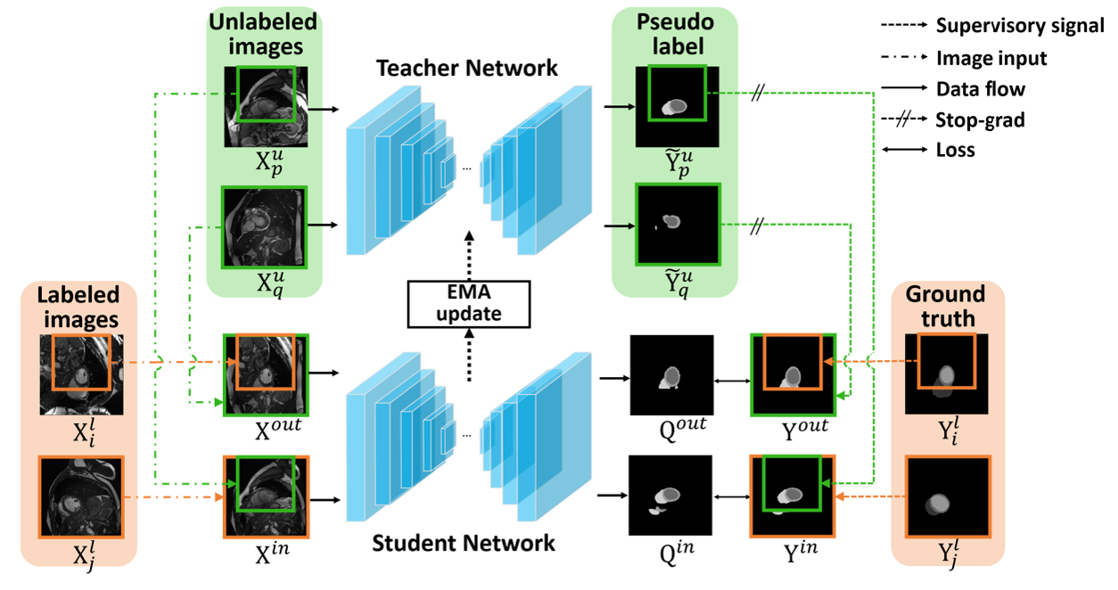
Figure 3: Overview of our bidirectional copy-paste framework in Mean Teacher architecture, drawn with 2D inputs for better visualization. The inputs to Student network are generated by mixing two labeled and two unlabeled images in the proposed bidirectional copy-paste manner. Then, to provide the supervisory signal to the Student network, we combine the ground-truths and the pseudo-labels generated by the Teacher network into one supervisory signal via the same bidirectional copy-paste, to enable strong supervision from ground-truths help the weak supervision from pseudo-label.

2.2 Semi-supervised Medical Image Segmentation

Many efforts have been made in semi-supervised medical image segmentation. Entropy minimization (EM) and consistency regularization (CR) are the two widely-used loss functions. Meanwhile, many works extended Mean Teacher framework in different ways. SASSNet [12] leveraged unlabeled data to enforce a geometric shape constraint on the segmentation output. DTC [16] proposed a dual-task-consistency framework by building task-level regularization explicitly. SimCVD [40] modeled geometric structure and semantic information explicitly and constrain them between Teacher and Student networks. These methods used geometric constraints to supervise the output of the network. UA-MT [41] used uncertainty information to guide Student network learn from the meaningful and reliable targets of Teacher network gradually. [46] combined image-wise and patch-wise representations to explore more complex similarity cues, enforcing the output to be consistent given different input sizes. CoraNet [22] proposed a model which can produce certain and uncertain regions, and Student network treats regions indicated from Teacher network with different weights. UMCT [37] used different perspectives of the network to predict the same image of different views. It utilized the predictions and the corresponding uncertainty to generate the pseudo-labels, which were used to supervise the prediction of unlabeled images. These methods have furthered the effectiveness for semi-supervised medical image segmentation. But, they ignored how to learn common semantics from labeled to unlabeled data. Treating labeled and unlabeled data separately often impedes knowledge transfer from labeled to unlabeled data.

2.3 Copy-Paste

Copy-paste is a simple but strong data processing method for many tasks, e.g., instance segmentation [9, 7], semantic segmentation [6, 25] and object detection [5]. Generally speaking, copy-paste means copying crops of one image and pasting them onto another image. Mixup [43] and CutMix [42] are classic works of mixing whole images and mixing image crops respectively. Many recent works extended them to address specific goals. GuidedMix-Net [25] used mixup to generate higher-quality pseudo-labels by transferring the knowledge of labeled data to the unlabeled data. InstaBoost [7] and Contextual Copy-Paste [5] placed the cropped foreground onto another image elaborately according to the surrounding visual context. CP² [27] proposed a pretraining method which copy-pastes a random crop from an image to another background image, it has been proved to be more suitable for downstream dense prediction tasks. [9] made a systematic study of copy-paste in instance segmentation. UCC [6] copied the pixels belonging to the class which has a low confidence score as foreground during training to alleviate the distribution mismatch and class imbalance problems. Previous methods only considered copy-paste cross unlabeled data, or simply copied crops from labeled data as foreground and pasted to another data. They neglect to design a consistent learning strategy for labeled and unlabeled data. Thus, a large distribution gap is still inevitable.

3 Method

Mathematically, we define the 3D volume of a medical image as $\textbf{X}\in\mathbb{R}^{W\times H\times L}$. The goal of semi-supervised medical image segmentation is to predict the per-voxel label map $\widehat{\textbf{Y}}\in\{0,1,...,K-1\}^{W\times H\times L}$, indicating where the background and the targets are in X. $K$ is the class number. Our training set $\mathcal{D}$ consists of $N$ labeled data and $M$ unlabeled data ($N\ll M$), expressed as two subsets: $\mathcal{D}=\mathcal{D}^{l}\cup\mathcal{D}^{u}$, where $\mathcal{D}^{l}=\{(\textbf{X}^{l}_{i},\textbf{Y}^{l}_{i})\}_{i=1}^{N}$ and $\mathcal{D}^{u}=\{\textbf{X}^{u}_{i}\}_{i=N+1}^{M+N}$.

The overall pipeline of the proposed bidirectional copy-paste method is shown in Fig. 3, in the Mean Teacher architecture. We randomly pick two unlabeled images $(\textbf{X}^{u}_{p},\textbf{X}^{u}_{q})$, and two labeled images $(\textbf{X}^{l}_{i},\textbf{X}^{l}_{j})$ from the training set. Then we copy-paste a random crop from $\textbf{X}^{l}_{i}$ (the foreground) onto $\textbf{X}^{u}_{q}$ (the background) to generate the mixed image $\textbf{X}^{out}$, and from $\textbf{X}^{u}_{p}$ (the foreground) onto $\textbf{X}^{l}_{j}$ (the background) to generate another mixed image $\textbf{X}^{in}$. Unlabeled images are able to learn comprehensive common semantics from labeled images from both inward ($\textbf{X}^{in}$) and outward ($\textbf{X}^{out}$) directions. Images $\textbf{X}^{in}$ and $\textbf{X}^{out}$ are then fed into the Student network to predict segmentation masks $\widehat{\textbf{Y}}^{in}$ and $\widehat{\textbf{Y}}^{out}$. The segmentation masks are supervised by bidirectional copy-pasting the predictions of the unlabeled images from the Teacher network and the label maps of the labeled images.

3.1 Bidirectional Copy-Paste

3.1.1 Mean-Teacher and Training Strategy

In our BCP framework, there are a Teacher network, $\mathcal{F}_{t}\left(\textbf{X}^{u}_{p},\textbf{X}^{u}_{q};\mathbf{\Theta}_{t}\right)$, and a Student network $\mathcal{F}_{s}\left(\textbf{X}^{in},\textbf{X}^{out};\mathbf{\Theta}_{s}\right)$, where $\mathbf{\Theta}_{t}$ and $\mathbf{\Theta}_{s}$ are parameters. The Student network is optimized by stochastic gradient descent, and the Teacher network is by exponential moving average (EMA) of Student network.[24] Our training strategy is divided into three steps. We first use only labeled data to pretrain a model, then we use the pretrained model as Teacher network to generate pseudo-labels for unlabeled images. At each iteration, we first optimize the Student network parameters $\mathbf{\Theta}_{s}$ by stochastic gradient descent. Finally, we update the Teacher network parameters $\mathbf{\Theta}_{t}$ using EMA of the Student parameters $\mathbf{\Theta}_{s}$.

3.1.2 Pre-Training via Copy-Paste

Inspired by previous work [9], we conducted Copy-Paste augmentation on labeled data to train a supervised model, the supervised model will generate pseudo-labels for unlabeled data during self-training. This strategy was proved to be effective to improve segmentation performance, more details will be illustrated in ablation studies.

3.1.3 Bidirectional Copy-Paste Images

To conduct copy-paste between a pair of images, we first generate a zero-centered mask $\mathcal{M}\in\{0,1\}^{W\times H\times L}$, indicating whether the voxel comes from the foreground ($0$) or the background ($1$) image. The size of the zero-value region is $\beta H\times\beta W\times\beta L$, where $\beta\in(0,1)$. Then we bidirectionally copy-paste labeled and unlabeled images as follows:

$$\textbf{X}^{in}=\textbf{X}^{l}_{j}\odot\mathcal{M}+\textbf{X}^{u}_{p}\odot\left(\textbf{1}-\mathcal{M}\right),$$ (1)

$$\textbf{X}^{out}=\textbf{X}^{u}_{q}\odot\mathcal{M}+\textbf{X}^{l}_{i}\odot\left(\textbf{1}-\mathcal{M}\right),$$ (2)

where $\textbf{X}^{l}_{i}$, $\textbf{X}^{l}_{j}\in\mathcal{D}^{l}$, $i\neq j$, $\textbf{X}^{u}_{p}$, $\textbf{X}^{u}_{q}\in\mathcal{D}^{u}$, $p\neq q$, $\textbf{1}\in\{1\}^{W\times H\times L}$, and $\odot$ means element-wise multiplication. Two labeled and unlabeled images are adopted to keep the diversity of the input.

3.1.4 Bidirectional Copy-Paste Supervisory Signals

To train the Student network, supervisory signals are also generated via BCP operation. Unlabeled images $\textbf{X}^{u}_{p}$ and $\textbf{X}^{u}_{q}$ are fed into the Teacher network, and their probability maps are computed:

$$\textbf{P}^{u}_{p}=\mathcal{F}_{t}(\textbf{X}^{u}_{p};\mathbf{\Theta}_{t}),~{}~{}~{}\textbf{P}^{u}_{q}=\mathcal{F}_{t}(\textbf{X}^{u}_{q};\mathbf{\Theta}_{t}).$$ (3)

The initial pseudo-label $\widehat{\textbf{Y}}^{u}$ ($p$ and $q$ are dropped for simplicity) are determined by taking a common threshold 0.5 on $\textbf{P}^{u}$ for binary segmentation tasks, or taking argmax operation on $\textbf{P}^{u}$ for multi-class segmentation tasks. The final pseudo-label $\widetilde{\textbf{Y}}^{u}$ is obtained via selecting the largest connected component of $\widehat{\textbf{Y}}^{u}$ which will effectively remove outlier voxels. Then, we propose to bidirectionally copy-paste the pseudo-labels of unlabeled images and ground truth labels of labeled images in the same manner as in Eq.1 and Eq.2 to obtain the supervisory signals:

$$\textbf{Y}^{in}=\textbf{Y}^{l}_{j}\odot\mathcal{M}+\widetilde{\textbf{Y}}^{u}_{p}\odot\left(\textbf{1}-\mathcal{M}\right),$$ (4)

$$\textbf{Y}^{out}=\widetilde{\textbf{Y}}^{u}_{q}\odot\mathcal{M}+\textbf{Y}^{l}_{i}\odot\left(\textbf{1}-\mathcal{M}\right).$$ (5)

$\textbf{Y}^{in}$ and $\textbf{Y}^{out}$ will be used as the supervision to supervise the Student network predictions of $\textbf{X}^{in}$ and $\textbf{X}^{out}$.

3.2 Loss Function

Each input image of the Student network consists of component from both labeled and unlabeled image. Intuitively, ground truth masks of labeled images are usually more accurate than pseudo-labels of unlabeled images. We use $\alpha$ to control the contribution of unlabeled image pixels to the loss function. The loss functions for $\textbf{X}^{in}$ and $\textbf{X}^{out}$ are computed respectively by

$$\mathcal{L}^{in}=\mathcal{L}_{\textit{seg}} \left(\textbf{Q}^{in},\textbf{Y}^{in}\right)\odot\mathcal{M}+$$ (6)

$$\alpha\mathcal{L}_{\textit{seg}}\left(\textbf{Q}^{in},\textbf{Y}^{in}\right)\odot\left(\textbf{1}-\mathcal{M}\right),$$

$$\mathcal{L}^{out}=\mathcal{L}_{\textit{seg}} \left(\textbf{Q}^{out},\textbf{Y}^{out}\right)\odot\left(\textbf{1}-\mathcal{M}\right)+$$ (7)

$$\alpha\mathcal{L}_{\textit{seg}}\left(\textbf{Q}^{out},\textbf{Y}^{out}\right)\odot\mathcal{M},$$

where $\mathcal{L}_{seg}$ is the linear combination of Dice loss and Cross-entropy loss. $\textbf{Q}^{in}$ and $\textbf{Q}^{out}$ are computed by:

$$\textbf{Q}^{in}=\mathcal{F}_{s}(\textbf{X}^{in};\mathbf{\Theta}_{s}),~{}~{}~{}\textbf{Q}^{out}=\mathcal{F}_{s}(\textbf{X}^{out};\mathbf{\Theta}_{s}).$$ (8)

At each iteration we update the parameters $\mathbf{\Theta}_{s}$ in Student network by stochastic gradient descent with the loss function:

$$\mathcal{L}_{\textit{all}}=\mathcal{L}^{in}+\mathcal{L}^{out}.$$ (9)

Afterwards, Teacher network parameters $\mathbf{\Theta}_{t}^{(k+1)}$ at the $\left(k+1\right)$th iteration are updated:

$$\mathbf{\Theta}_{t}^{(k+1)}=\lambda\mathbf{\Theta}_{t}^{(k)}+\left(1-\lambda\right)\mathbf{\Theta}_{s}^{(k)},$$ (10)

where $\lambda$ is the smoothing coefficient parameter.

3.3 Testing Phase

In the testing stage, given a testing image $\textbf{X}_{test}$, we obtain the probability map by: $\textbf{Q}_{test}=\mathcal{F}(\textbf{X}_{test};\widehat{\mathbf{\Theta}}_{s})$, where $\widehat{\mathbf{\Theta}}_{s}$ are the well-trained Student network parameters. The final label map can be easily determined by $\textbf{Q}_{test}$.

Method	Scans used		Metrics
	Labeled	Unlabeled	Dice$\uparrow$	Jaccard$\uparrow$	95HD$\downarrow$	ASD$\downarrow$
V-Net	4(5%)	0	52.55	39.60	47.05	9.87
V-Net	8(10%)	0	82.74	71.72	13.35	3.26
V-Net	80(All)	0	91.47	84.36	5.48	1.51
UA-MT	4(5%)	76(95%)	82.26	70.98	13.71	3.82
SASSNet			81.60	69.63	16.16	3.58
DTC			81.25	69.33	14.90	3.99
URPC			82.48	71.35	14.65	3.65
MC-Net			83.59	72.36	14.07	2.70
SS-Net			86.33	76.15	9.97	2.31
Ours			88.02$\uparrow$1.69	78.72$\uparrow$2.57	7.90$\downarrow$2.07	2.15$\downarrow$0.16
UA-MT	8(10%)	72(90%)	87.79	78.39	8.68	2.12
SASSNet			87.54	78.05	9.84	2.59
DTC			87.51	78.17	8.23	2.36
URPC			86.92	77.03	11.13	2.28
MC-Net			87.62	78.25	10.03	1.82
SS-Net			88.55	79.62	7.49	1.90
Ours			89.62$\uparrow$1.07	81.31$\uparrow$1.69	6.81$\downarrow$0.68	1.76$\downarrow$0.14

Table 1: Comparisons with state-of-the-art semi-supervised segmentation methods on LA dataset. Improvements compared with the second best results are highlighted.

4 Experiments

4.1 Dataset

LA dataset. Atrial Segmentation Challenge [39] dataset includes 100 3D gadolinium-enhanced magnetic resonance image scans (GE-MRIs) with labels. We strictly follow the setting used in SSNet [35], DTC [16] and UA-MT [41].

Pancreas-NIH. Pancreas-NIH [21] dataset contains 82 contrast-enhanced abdominal CT volumes which are manually delineated. For fair comparison, we follow the setting in CoraNet [22].

ACDC dataset. ACDC [2] dataset is a four-class (i.e. background, right ventricle, left ventricle and myocardium) segmentation dataset, containing 100 patients’ scans. The data split [15] is fixed with 70, 10, and 20 patients’ scans for training, validation, and testing.

4.2 Evaluation Metrics

We choose four evaluation metrics: Dice Score (%), Jaccard Score (%), 95% Hausdorff Distance (95HD) in voxel and Average Surface Distance (ASD) in voxel. Given two object regions, Dice and Jaccard mainly compute the percentage of overlap between them, ASD computes the average distance between their boundaries, and 95HD measures the closest point distance between them.

4.3 Implementation Details

$\alpha=0.5,\beta=2/3$ are set as the default value in experiments, unless otherwise specified. We conduct all experiments on an NVIDIA 3090 GPU with fixed random seeds.

Method	Scans used		Metrics
	Labeled	Unlabeled	Dice$\uparrow$	Jaccard$\uparrow$	95HD$\downarrow$	ASD$\downarrow$
V-Net	12(20%)	50(80%)	69.96	55.55	14.27	1.64
DAN			76.74	63.29	11.13	2.97
ADVNET			75.31	61.73	11.72	3.88
UA-MT			77.26	63.82	11.90	3.06
SASSNet			77.66	64.08	10.93	3.05
DTC			78.27	64.75	8.36	2.25
CoraNet			79.67	66.69	7.59	1.89
Ours			82.91$\uparrow$3.24	70.97$\uparrow$4.28	6.43$\downarrow$1.16	2.25$\uparrow$0.61

Table 2: Comparisons with state-of-the-art semi-supervised segmentation methods on the Pancreas-NIH dataset.

Method	Scans used		Metrics
	Labeled	Unlabeled	Dice$\uparrow$	Jaccard$\uparrow$	95HD$\downarrow$	ASD$\downarrow$
U-Net	3(5%)	0	47.83	37.01	31.16	12.62
U-Net	7(10%)	0	79.41	68.11	9.35	2.70
U-Net	70(All)	0	91.44	84.59	4.30	0.99
UA-MT	3(5%)	67(95%)	46.04	35.97	20.08	7.75
SASSNet			57.77	46.14	20.05	6.06
DTC			56.90	45.67	23.36	7.39
URPC			55.87	44.64	13.60	3.74
MC-Net			62.85	52.29	7.62	2.33
SS-Net			65.83	55.38	6.67	2.28
Ours			87.59$\uparrow$21.76	78.67$\uparrow$23.29	1.90$\downarrow$4.77	0.67$\downarrow$1.61
UA-MT	7(10%)	63(90%)	81.65	70.64	6.88	2.02
SASSNet			84.50	74.34	5.42	1.86
DTC			84.29	73.92	12.81	4.01
URPC			83.10	72.41	4.84	1.53
MC-Net			86.44	77.04	5.50	1.84
SS-Net			86.78	77.67	6.07	1.40
Ours			88.84$\uparrow$2.06	80.62$\uparrow$2.95	3.98$\downarrow$2.09	1.17$\downarrow$0.23

Table 3: Comparisons with state-of-the-art semi-supervised segmentation methods on the ACDC dataset.

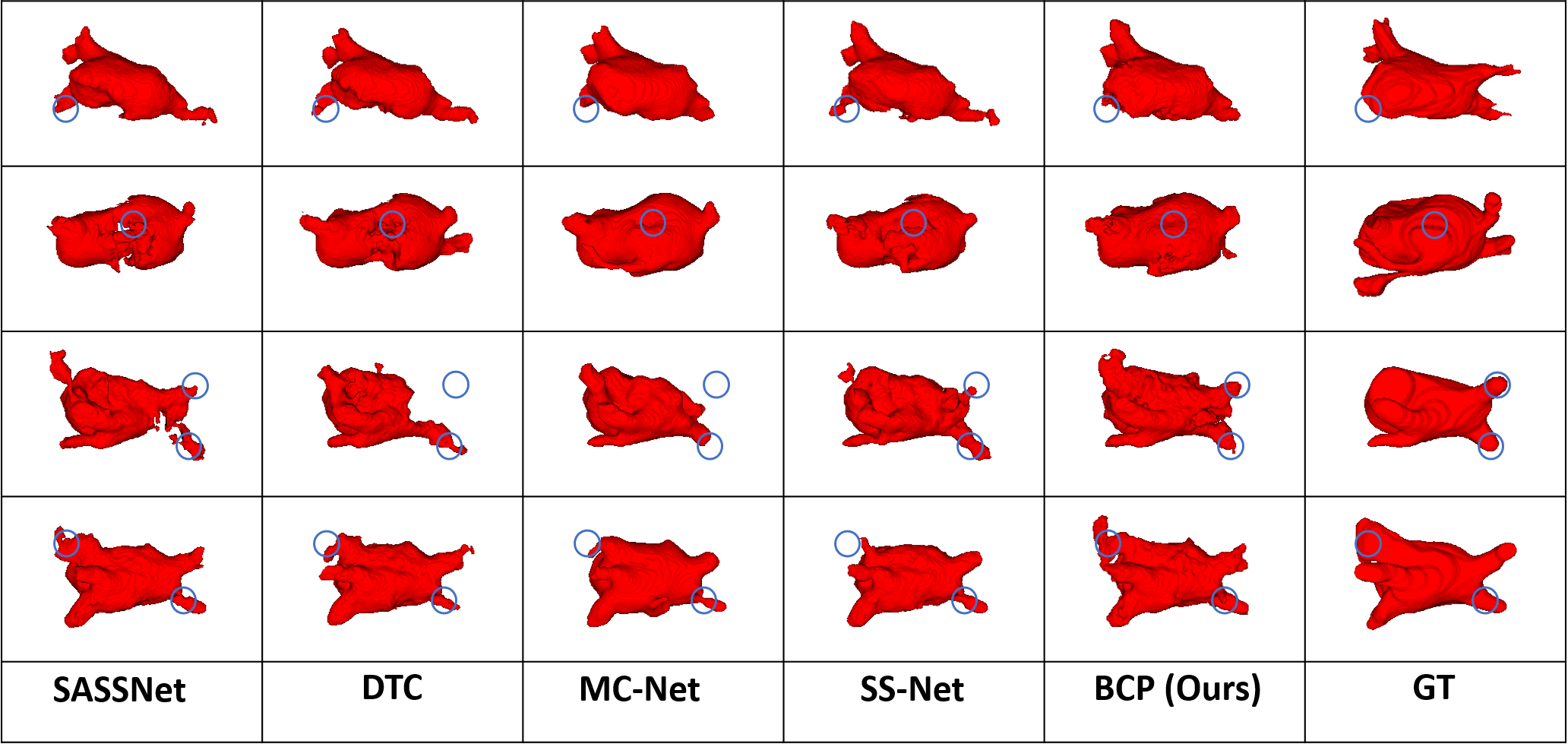
Figure 4: Visualizations of several semi-supervised segmentation methods with 10% labeled data and ground truth on LA dataset (best viewed by zoom-in on screen).

Method	LA						ACDC
	Scans used		Metrics				Scans used		Metrics
	Labeled	Unlabeled	Dice$\uparrow$	Jaccard$\uparrow$	95HD$\downarrow$	ASD$\downarrow$	Labeled	Unlabeled	Dice$\uparrow$	Jaccard$\uparrow$	95HD$\downarrow$	ASD$\downarrow$
In	4(5%)	76(95%)	87.35	77.77	8.75	2.21	3(5%)	67(95%)	81.68	70.07	4.69	1.28
Out			87.32	77.78	9.38	2.16			72.19	60.69	39.57	18.15
CP			79.67	67.05	14.66	3.21			81.80	71.70	16.29	6.43
Ours			88.02	78.72	7.90	2.15			87.59	78.67	1.90	0.67
In	8(10%)	72(90%)	89.02	80.38	8.08	1.81	7(10%)	63(90%)	85.55	75.65	4.93	1.50
Out			87.61	78.10	8.99	2.63			87.23	78.07	8.61	2.39
CP			86.74	77.18	8.65	2.26			88.17	79.64	6.14	1.45
Ours			89.62	81.31	6.81	1.76			88.84	80.62	3.98	1.17

Table 4: Ablation study of the copy-paste directions. In: inward copy-paste (foreground: unlabeled, background: labeled). Out: outward copy-paste (foreground: labeled, background: unlabeled). CP: direct copy-paste (background & foreground: labeled & labeled and unlabeled & unlabeled).

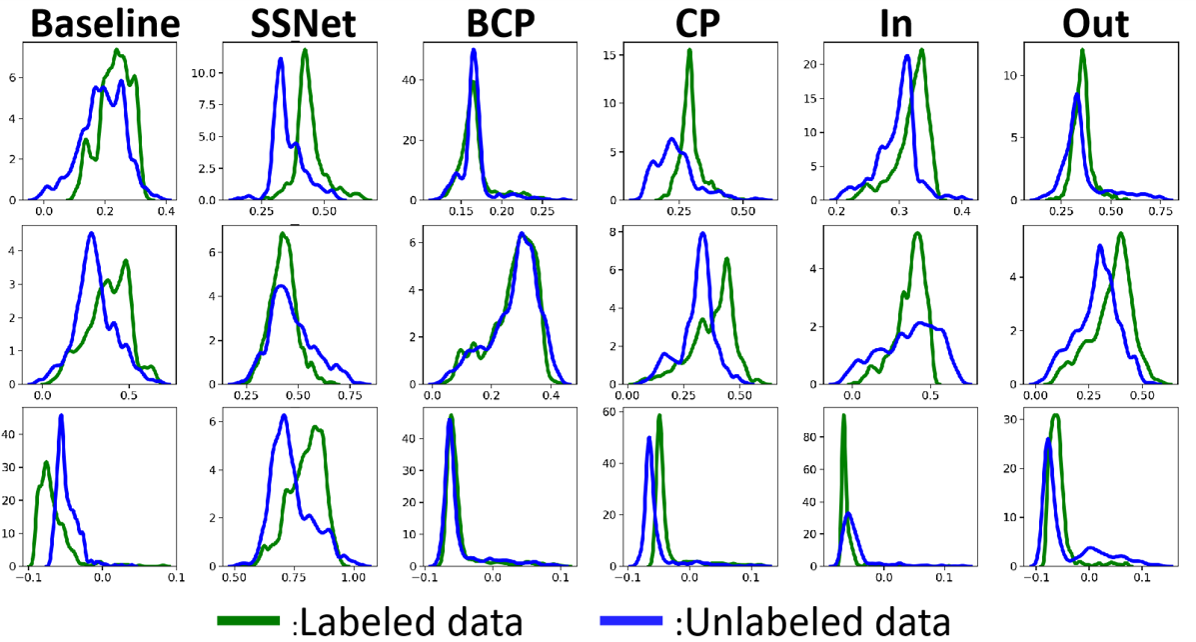
Figure 5: Kernel dense estimations of different methods, trained on 10% labeled ACDC dataset. Top to bottom are kernel dense estimations of features belong to three different class of ACDC: right ventricle, myocardium and left ventricle. Baseline: Only labeled data are used to train the network. CP, In and Out are same as Table 4. It can be seen that our BCP could make the features of labeled data and unlabeled data align better. Furthermore, the outstanding performance of our method compared with In and Out demonstrates the necessity of bidirectional copy-paste.

Method	Scans used		Metrics
	Labeled	Unlabeled	Dice$\uparrow$	Jaccard$\uparrow$	95HD$\downarrow$	ASD$\downarrow$
Mixup	4(5%)	76(95%)	41.71	29.58	59.75	21.87
FG-CutMix			67.05	54.00	30.52	6.15
Ours			88.02	78.72	7.90	2.15
Mixup	8(10%)	72(90%)	63.64	52.51	21.67	3.61
FG-CutMix			83.58	72.70	11.96	2.56
Ours			89.62	81.31	6.81	1.76

Table 5: Ablation study of interpolation strategies on LA dataset. Mixup: We imitate the framework of GuidedMix-Net[25], which is proposed for semi-supervised segmentation of natural images. FG-CutMix: We crop images of the whole training batch into 4$\times$4 patches and then combine them randomly to generate new images.

LA dataset. Following SS-Net [35], we use rotation and flip operations to augment data and train our model via an SGD optimizer with the initial learning rate 0.01 decay by 10% every 2.5K iterations. The backbone is set as 3D V-Net. During training, we randomly crop $112\times 112\times 80$ patches, and the size of the zero-value region is $74\times 74\times 53$ ($\beta=2/3$). The batch size is set as 8, containing four labeled patches and four unlabeled patches. The iterations of pre-training and self-training are set as 2k and 15k respectively.

Pancreas-NIH. Following CoraNet [22], we augment data by rotating, rescaling and flipping, and train a four-layer 3D V-Net by Adam optimizer with initial learning rate as 0.001. During training, we randomly crop $96\times 96\times 96$ patches input the network, the size of the zero-value region of mask $\mathcal{M}$ is $64\times 64\times 64$. We set the batch size, pre-training epochs and the self-training epochs as 8, 60 and 200 respectively.

ACDC dataset. Following SS-Net [35], we use 2D U-Net as the backbone of our experiments. During training, the input patch size is $256\times 256$ (2D slices) and the size of the zero-value region of mask $\mathcal{M}$ is $170\times 170$. The batch size, pre-training iterations, and the self-training training iterations are set as 24, 10k and 30k respectively.

4.4 Comparison with Sate-of-the-Art Methods

LA dataset

We compare our framework on LA dataset with various competitors: UA-MT [41], SASSNet [12], DTC [16], URPC [17], MC-Net [36] and SS-Net [35]. Following SS-Net, semi-supervised experiments of different labeled ratios (i.e. 5% and 10%) are carried out. Results from other competitors were reported in the identical experimental setting in SS-Net [35] for fair comparisons. As shown in Table 1, our method achieves the best performance on all four evaluation metrics, outperforming other competitors by a big margin. Thanks to BCP, the network “sees” more variances for boundary regions or semantic change of voxels, allowing for achieving good shape-related performances (see 95HD and ASD) without any explicit boundary or shape constraints during training. Moreover, it can be seen in Fig. 4 that our method can segment fine details of the target organ, especially edges that are easy to be misidentified (the first row) or missed (the second, third and fourth row), highlighted by blue circles.

Pancreas-NIH dataset

We conduct experiments on Pancreas-NIH dataset with 20% labeled ratio [16, 22]. We compared BCP with V-Net [19], DAN [44], ADVNET [26], UA-MT [41], SASSNet [12], DTC [16] and CoraNet [22] in Table 2. In this table, DAN, ADVNET, UA-MT, SASSNet, DTC, CoraNet and our method took both labeled and unlabeled data to train the network with V-Net as the backbone, while V-Net only uses labeled data in the supervised setting (lower bound). BCP achieves significant improvement on Dice, Jaccard and 95HD (i.e., surpassing the second best by 3.24%, 4.28% and 1.16, respectively). These results do not conduct any post-processing for fair comparison.

Mode	Scans used		Metrics
	Labeled	Unlabeled	Dice$\uparrow$	Jaccard$\uparrow$	95HD$\downarrow$	ASD$\downarrow$
Random	4(5%)	76(95%)	86.15	76.03	9.19	2.38
Contact			86.64	76.32	9.61	2.58
Ours			88.02	78.72	7.90	2.15
Random	8(10%)	72(90%)	84.50	73.79	10.79	2.39
Contact			88.66	79.82	7.93	2.27
Ours			89.62	81.31	6.81	1.76

Table 6: Results with three masking strategies on LA dataset.

ACDC dataset

Table 3 shows the averaged performance of four-class segmentation results on ACDC dataset with 5% and 10% labeled ratios. BCP surpasses all state-of-the-arts. We obtain a huge performance improvement up to 21.76% in terms of Dice for the setting with 5% labeled ratio. Following SS-Net [35], 2D slices are used to train our network. Noted that one 3D volume can be sliced into many 2D slices, so much more combinations from labeled and unlabeled slices could be produced than those using 3D data. Hence, during training, the knowledge of labeled data can be transferred to unlabeled data more sufficiently, especially when the number of labeled volume is very small. This might be the reason for such a significant improvement compared with others when the labeled ratio is 5%.

4.5 Ablation Studies

We conduct ablation studies to show the impact of each component in BCP. Including CP directions, design choices of masking strategies, interpolation strategies, $\beta$ (size ratio for zero-value region in $\mathcal{M}$), and $\alpha$ (Eq. 6-7). We also investigate step-by-step the significant improvement of our method compared with competitors on the ACDC dataset with 5% labeled ratio. Some ablation studies on ACDC dataset are shown in the supplementary material.

$\beta$	Scans used		Metrics
	Labeled	Unlabeled	Dice$\uparrow$	Jaccard$\uparrow$	95HD$\downarrow$	ASD$\downarrow$
1/3	4(5%)	76(95%)	79.92	67.73	15.44	3.63
1/2			86.49	76.63	8.74	2.23
2/3			88.02	78.72	7.90	2.15
5/6			87.92	78.57	8.29	2.26
1/3	8(10%)	72(90%)	83.20	72.04	11.64	2.94
1/2			88.81	89.10	7.33	1.96
2/3			89.62	81.31	6.81	1.76
5/6			88.75	79.96	7.63	2.07

Table 7: Ablation study of $\beta$ on LA dataset.

$\alpha$	LA						ACDC
	Scans used		Metrics				Scans used		Metrics
	Labeled	Unlabeled	Dice$\uparrow$	Jaccard$\uparrow$	95HD$\downarrow$	ASD$\downarrow$	Labeled	Unlabeled	Dice$\uparrow$	Jaccard$\uparrow$	95HD$\downarrow$	ASD$\downarrow$
0.5	4(5%)	76(95%)	88.02	78.72	7.90	2.15	3(5%)	67(95%)	87.59	78.67	1.90	0.67
1.5			87.21	77.49	8.67	2.37			85.88	76.02	3.17	0.93
2.5			86.56	76.46	9.82	2.60			85.43	75.47	12.02	4.05
0.5	8(10%)	72(90%)	89.62	81.31	6.81	1.76	7(10%)	63(90%)	88.84	80.62	3.98	1.17
1.5			89.35	80.88	7.46	2.09			88.65	80.31	1.99	0.68
2.5			88.74	79.88	7.73	2.15			87.13	78.19	3.67	1.24

Table 8: Ablation study of the weights $\alpha$ in the loss function.

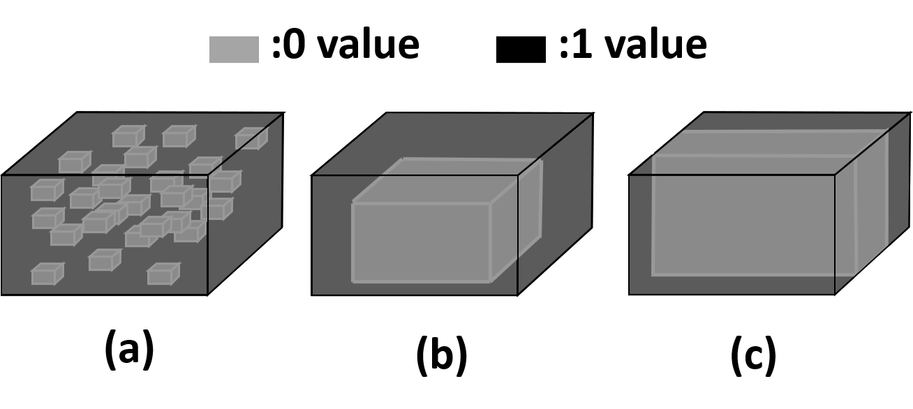
Figure 6: Different masking strategies. (a): random mask; (b): zero-centered mask; (c): contact mask.

Copy-Paste Direction

We design three experiments to investigate the influence of different copy-paste directions in Table 4. Inward and outward copy-paste (In and Out in the table) mean using $\textbf{X}^{l}\odot\mathcal{M}+\textbf{X}^{u}\odot\left(\textbf{1}-\mathcal{M}\right)$ or $\textbf{X}^{u}\odot\mathcal{M}+\textbf{X}^{l}\odot\left(\textbf{1}-\mathcal{M}\right)$ respectively to train the network. We also conduct within-set copy-paste (CP in the table), i.e., copy-paste labeled data on another labeled data and copy-paste unlabeled data on another unlabeled data. We can see that all these variants get inferior performances compared with our BCP, since they either lack consistent manner for training labeled and unlabeled data, or lack common semantics transfer between labeled and unlabeled data.

Interpolation Strategies

We compare BCP with other two interpolation strategies: Mixup [43] and Fine-Grained CutMix (FG-CutMix). For Mixup, we superimpose labeled and unlabeled data to generate new training images, imitating the framework of GuidedMix-Net [25]. For FG-CutMix, we crop training images into 4$\times$4 patches and combine them in batch to generate new images. The network predictions of new images are re-combined and then supervised by ground-truth or pseudo-labels. The results of LA dataset are shown in Table 5. Due to similar spatial structures of medical images, Mixup brings more influential noise in medical images. FG-CutMix maintains less structure information after CutMix than BCP. More details will be discussed in supplementary material.

Strategy	Scans used		Metrics
	Labeled	Unlabeled	Dice$\uparrow$	Jaccard$\uparrow$	95HD$\downarrow$	ASD$\downarrow$
random	4(5%)	76(95%)	86.06	75.96	9.48	2.33
w/o CP			86.46	76.50	8.93	2.31
Ours			88.02	78.72	7.90	2.15
random	8(10%)	72(90%)	87.93	78.67	8.24	2.08
w/o CP			88.75	79.88	7.66	1.83
Ours			89.62	81.31	6.81	1.76

Table 9: Ablation study of pre-training strategy on LA dataset. random: Initialized randomly. w/o CP: Initialized from a pre-trained model trained on labeled data without copy-paste.

Design Choices of Masking Strategies

As shown in Fig. 6, we explore different masking strategies in BCP on LA dataset. To conduct a fair comparison, we maintain the same number of zero-value voxels for different strategies. We randomly sample 27 small $\beta H\times\beta W\times\beta L$ zero-value cubes in an all-one mask, and set $\beta=2/9$ for each zero-value cube. For contact mask, the shape of zero-value region is $\beta H\times W\times L$, and $\beta$ is set as 8/27 to control the number of zero-value voxels. As shown in Table 6, random mask obtains worst performance, since small random cubes only contain incoherently local foreground of an image, which lacks the ability in learning complete foreground representation. Contact mask has better integrity of foreground information, which performs better than random mask, but still performs worse than zero-centered mask used in our method, since foreground has less chance interacting with the background, compared with zero-centered mask. Thus, both random mask and contact mask have weaker ability in mitigating the distribution mismatch problem between labeled and unlabeled data.

Size of Zero-value Region in M

We study the impact of zero-value region size on LA dataset, as shown in the Table 7. For the zero-value region $\beta H\times\beta W\times\beta L$ in the mask $\mathcal{M}$, we set $\beta=\{\frac{1}{3},\frac{1}{2},\frac{2}{3},\frac{5}{6}\}$. The performance gets worse as $\beta$ decreases, which means small copy-pasted foreground has limited ability in transferring common semantics to/from the background. Best performance is achieved when $\beta=2/3$ and it decreases a bit when $\beta=5/6$.

Weight in Loss Function

We set $\alpha=0.5$ as the default value. Now we vary $\alpha=\{0.5,1.5,2.5\}$ to see how the performance changes. Table 8 shows it is not sensitive when $\alpha$ changes from 0.5 to 1.5, but an obvious performance drop is observed when $\alpha=2.5$.

BCP	nms	Pre-Train	Dice$\uparrow$	Jaccard$\uparrow$	95HD$\downarrow$	ASD$\downarrow$
			47.62	36.61	29.02	11.46
✓			83.26	72.71	23.90	7.49
✓	✓		82.33	72.76	9.78	4.74
✓	✓	✓	87.59	78.67	1.90	0.67

Table 10: Ablation on ACDC dataset with 5% labeled data, $\alpha=0.5$ across all experiments. nms: Post-processing the pseudo-labels for unlabeled data. Pre-Train: Initialized from a pre-trained model with copy-paste on labeled data.

Teacher Network Initialization Strategy

In our default setting, the Teacher network is initialized by a pre-trained model, which is trained on labeled data in a copy-paste manner. We study other network initialization strategies: initialized randomly and initialized from a pre-trained model which is trained on labeled data without copy-paste. Comparison results are shown in Table 9. Compared with pre-training on original labeled data, performing copy-paste on the labeled data during pre-train can effectively improve the generalization ability of the network.

Ablation on ACDC with 5% Labeled Data

In Table 3, our method achieves a huge improvement on ACDC dataset with 5% labeled data. We separate our method into three components and study which component contributes the most to this improvement. As shown in Table 10, without our component (the first row), it degenerated into a normal pseudo-label-based self-training method, which means the segmentation of labeled and unlabeled images are supervised by ground truth and pseudo-labels respectively. Then, BCP leads to a significant performance gain (from 47.62% to 83.26% in Dice). Post-processing (nms) and a better Teacher network initialization enhance the quality of pseudo-labels and thus further improve the performance.

5 Conclusion

We have presented the bidirectional copy-paste (BCP) for semi-supervised medical image segmentation. We extend copy-paste-based method in a bidirectional manner, which reduces the distribution gap between labeled and unlabeled data. Experiments on LA, NIH-Pancreas and ACDC datasets show the superiority of the proposed BCP, with even over 21% Dice improvement on ACDC dataset with 5% labeled data. Note that BCP does not introduce new parameters or computational cost compared with the backbone network. Limitations. We didn’t specifically design a module to enhance local attributes learning. Though BCP performs better than all competitors, target parts with extremely low contrast are still hard to segment well (e.g., bottom left part on $2$nd row of Fig. 4 is missing).

6 Acknowledgement

This work was supported by the National Natural Science Foundation of China (Grant No. 62101191), Shanghai Natural Science Foundation (Grant No. 21ZR1420800), the Science and Technology Commission of Shanghai Municipality (Grant No. 22DZ2229004), and the Fundamental Research Funds for the Central Universities.

References

- [1] Wenjia Bai, Ozan Oktay, Matthew Sinclair, Hideaki Suzuki, Martin Rajchl, Giacomo Tarroni, Ben Glocker, Andrew P. King, Paul M. Matthews, and Daniel Rueckert. Semi-supervised learning for network-based cardiac MR image segmentation. In Proc. MICCAI, 2017.
- [2] Olivier Bernard, Alain Lalande, Clément Zotti, Frederic Cervenansky, Xin Yang, Pheng-Ann Heng, Irem Cetin, Karim Lekadir, Oscar Camara, Miguel Ángel González Ballester, Gerard Sanroma, Sandy Napel, Steffen E. Petersen, Georgios Tziritas, Elias Grinias, Mahendra Khened, Alex Varghese, Ganapathy Krishnamurthi, Marc-Michel Rohé, Xavier Pennec, Maxime Sermesant, Fabian Isensee, Paul Jaeger, Klaus H. Maier-Hein, Peter M. Full, Ivo Wolf, Sandy Engelhardt, Christian F. Baumgartner, Lisa M. Koch, Jelmer M. Wolterink, Ivana Isgum, Yeonggul Jang, Yoonmi Hong, Jay Patravali, Shubham Jain, Olivier Humbert, and Pierre-Marc Jodoin. Deep learning techniques for automatic MRI cardiac multi-structures segmentation and diagnosis: Is the problem solved? IEEE Trans. Medical Imaging, 37(11):2514–2525, 2018.
- [3] Özgün Çiçek, Ahmed Abdulkadir, Soeren S. Lienkamp, Thomas Brox, and Olaf Ronneberger. 3d u-net: Learning dense volumetric segmentation from sparse annotation. In Proc. MICCAI, 2016.
- [4] Qi Dou, Quande Liu, Pheng-Ann Heng, and Ben Glocker. Unpaired multi-modal segmentation via knowledge distillation. IEEE Trans. Medical Imaging, 39(7):2415–2425, 2020.
- [5] Nikita Dvornik, Julien Mairal, and Cordelia Schmid. Modeling visual context is key to augmenting object detection datasets. In Proc. ECCV, 2018.
- [6] Jiashuo Fan, Bin Gao, Huan Jin, and Lihui Jiang. UCC: uncertainty guided cross-head co-training for semi-supervised semantic segmentation. In Proc. CVPR, 2022.
- [7] Haoshu Fang, Jianhua Sun, Runzhong Wang, Minghao Gou, Yonglu Li, and Cewu Lu. Instaboost: Boosting instance segmentation via probability map guided copy-pasting. In Proc. ICCV, 2019.
- [8] Geoffrey French, Samuli Laine, Timo Aila, Michal Mackiewicz, and Graham D. Finlayson. Semi-supervised semantic segmentation needs strong, varied perturbations. In 31st British Machine Vision Conference 2020, BMVC 2020, Virtual Event, UK, September 7-10, 2020. BMVA Press, 2020.
- [9] Golnaz Ghiasi, Yin Cui, Aravind Srinivas, Rui Qian, Tsung-Yi Lin, Ekin D. Cubuk, Quoc V. Le, and Barret Zoph. Simple copy-paste is a strong data augmentation method for instance segmentation. In Proc. CVPR, 2021.
- [10] Jongmok Kim, Jooyoung Jang, Seunghyeon Seo, Jisoo Jeong, Jongkeun Na, and Nojun Kwak. MUM : Mix image tiles and unmix feature tiles for semi-supervised object detection. CoRR, abs/2111.10958, 2021.
- [11] Jiwon Kim, Kwangrok Ryoo, Junyoung Seo, Gyuseong Lee, Daehwan Kim, Hansang Cho, and Seungryong Kim. Semi-supervised learning of semantic correspondence with pseudo-labels. In IEEE/CVF Conference on Computer Vision and Pattern Recognition, CVPR 2022, New Orleans, LA, USA, June 18-24, 2022, pages 19667–19677. IEEE, 2022.
- [12] Shuailin Li, Chuyu Zhang, and Xuming He. Shape-aware semi-supervised 3d semantic segmentation for medical images. In Proc. MICCAI, 2020.
- [13] Xiaomeng Li, Hao Chen, Xiaojuan Qi, Qi Dou, Chi-Wing Fu, and Pheng-Ann Heng. H-denseunet: Hybrid densely connected unet for liver and tumor segmentation from CT volumes. IEEE Trans. Medical Imaging, 37(12):2663–2674, 2018.
- [14] Yuyuan Liu, Yu Tian, Yuanhong Chen, Fengbei Liu, Vasileios Belagiannis, and Gustavo Carneiro. Perturbed and strict mean teachers for semi-supervised semantic segmentation. CoRR, abs/2111.12903, 2021.
- [15] Xiangde Luo. SSL4MIS. https://github.com/HiLab-git/SSL4MIS, 2020.
- [16] Xiangde Luo, Jieneng Chen, Tao Song, and Guotai Wang. Semi-supervised medical image segmentation through dual-task consistency. In Proc. AAAI, 2021.
- [17] Xiangde Luo, Wenjun Liao, Jieneng Chen, Tao Song, Yinan Chen, Shichuan Zhang, Nianyong Chen, Guotai Wang, and Shaoting Zhang. Efficient semi-supervised gross target volume of nasopharyngeal carcinoma segmentation via uncertainty rectified pyramid consistency. In Medical Image Computing and Computer Assisted Intervention - MICCAI 2021 - 24th International Conference, Strasbourg, France, September 27 - October 1, 2021, Proceedings, Part II, volume 12902 of Lecture Notes in Computer Science, pages 318–329. Springer, 2021.
- [18] Fausto Milletari, Nassir Navab, and Seyed-Ahmad Ahmadi. V-net: Fully convolutional neural networks for volumetric medical image segmentation. In Proc. 3DV, 2016.
- [19] Fausto Milletari, Nassir Navab, and Seyed-Ahmad Ahmadi. V-net: Fully convolutional neural networks for volumetric medical image segmentation. In Fourth International Conference on 3D Vision, 3DV 2016, Stanford, CA, USA, October 25-28, 2016, pages 565–571. IEEE Computer Society, 2016.
- [20] Olaf Ronneberger, Philipp Fischer, and Thomas Brox. U-net: Convolutional networks for biomedical image segmentation. In Proc. MICCAI, 2015.
- [21] Holger R. Roth, Le Lu, Amal Farag, Hoo-Chang Shin, Jiamin Liu, Evrim B. Turkbey, and Ronald M. Summers. Deeporgan: Multi-level deep convolutional networks for automated pancreas segmentation. In Medical Image Computing and Computer-Assisted Intervention - MICCAI 2015 - 18th International Conference Munich, Germany, October 5-9, 2015, Proceedings, Part I, volume 9349 of Lecture Notes in Computer Science, pages 556–564. Springer, 2015.
- [22] Yinghuan Shi, Jian Zhang, Tong Ling, Jiwen Lu, Yefeng Zheng, Qian Yu, Lei Qi, and Yang Gao. Inconsistency-aware uncertainty estimation for semi-supervised medical image segmentation. IEEE Trans. Medical Imaging, 41(3):608–620, 2022.
- [23] Youbao Tang, Jinzheng Cai, Ke Yan, Lingyun Huang, Guotong Xie, Jing Xiao, Jingjing Lu, Gigin Lin, and Le Lu. Weakly-supervised universal lesion segmentation with regional level set loss. In Proc. MICCAI, 2021.
- [24] Antti Tarvainen and Harri Valpola. Mean teachers are better role models: Weight-averaged consistency targets improve semi-supervised deep learning results. In Proc. NIPS, 2017.
- [25] Peng Tu, Yawen Huang, Feng Zheng, Zhenyu He, Liujuan Cao, and Ling Shao. Guidedmix-net: Semi-supervised semantic segmentation by using labeled images as reference. In Proc. AAAI, 2022.
- [26] Tuan-Hung Vu, Himalaya Jain, Maxime Bucher, Matthieu Cord, and Patrick Pérez. ADVENT: adversarial entropy minimization for domain adaptation in semantic segmentation. In IEEE Conference on Computer Vision and Pattern Recognition, CVPR 2019, Long Beach, CA, USA, June 16-20, 2019, pages 2517–2526. Computer Vision Foundation / IEEE, 2019.
- [27] Feng Wang, Huiyu Wang, Chen Wei, Alan L. Yuille, and Wei Shen. CP2: copy-paste contrastive pretraining for semantic segmentation. In Proc. ECCV, 2022.
- [28] Fakai Wang, Kang Zheng, Le Lu, Jing Xiao, Min Wu, and Shun Miao. Automatic vertebra localization and identification in CT by spine rectification and anatomically-constrained optimization. In Proc. CVPR, 2021.
- [29] Jiacheng Wang, Xiaomeng Li, Yiming Han, Jing Qin, Liansheng Wang, and Qichao Zhou. Separated contrastive learning for organ-at-risk and gross-tumor-volume segmentation with limited annotation. In Proc. AAAI, 2022.
- [30] Qin Wang, Wen Li, and Luc Van Gool. Semi-supervised learning by augmented distribution alignment. In 2019 IEEE/CVF International Conference on Computer Vision, ICCV 2019, Seoul, Korea (South), October 27 - November 2, 2019, pages 1466–1475. IEEE, 2019.
- [31] Xuehui Wang, Kai Zhao, Ruixin Zhang, Shouhong Ding, Yan Wang, and Wei Shen. Contrastmask: Contrastive learning to segment every thing. In Proc. CVPR, 2022.
- [32] Yidong Wang, Hao Chen, Qiang Heng, Wenxin Hou, Yue Fan, Zhen Wu, Marios Savvides, Takahiro Shinozaki, Bhiksha Raj, and Bernt Schiele. Freematch: Self-adaptive thresholding for semi-supervised learning. CoRR, abs/2205.07246, 2022.
- [33] Yan Wang, Xu Wei, Fengze Liu, Jieneng Chen, Yuyin Zhou, Wei Shen, Elliot K. Fishman, and Alan L. Yuille. Deep distance transform for tubular structure segmentation in CT scans. In Proc. CVPR, 2020.
- [34] Yan Wang, Yuyin Zhou, Wei Shen, Seyoun Park, Elliot K. Fishman, and Alan L. Yuille. Abdominal multi-organ segmentation with organ-attention networks and statistical fusion. Medical Image Anal., 55:88–102, 2019.
- [35] Yicheng Wu, Zhonghua Wu, Qianyi Wu, Zongyuan Ge, and Jianfei Cai. Exploring smoothness and class-separation for semi-supervised medical image segmentation. CoRR, abs/2203.01324, 2022.
- [36] Yicheng Wu, Minfeng Xu, Zongyuan Ge, Jianfei Cai, and Lei Zhang. Semi-supervised left atrium segmentation with mutual consistency training. In Medical Image Computing and Computer Assisted Intervention - MICCAI 2021 - 24th International Conference, Strasbourg, France, September 27 - October 1, 2021, Proceedings, Part II, volume 12902 of Lecture Notes in Computer Science, pages 297–306. Springer, 2021.
- [37] Yingda Xia, Dong Yang, Zhiding Yu, Fengze Liu, Jinzheng Cai, Lequan Yu, Zhuotun Zhu, Daguang Xu, Alan L. Yuille, and Holger Roth. Uncertainty-aware multi-view co-training for semi-supervised medical image segmentation and domain adaptation. Medical Image Anal., 65:101766, 2020.
- [38] Lingxi Xie, Qihang Yu, Yuyin Zhou, Yan Wang, Elliot K. Fishman, and Alan L. Yuille. Recurrent saliency transformation network for tiny target segmentation in abdominal CT scans. IEEE Trans. Medical Imaging, 39(2):514–525, 2020.
- [39] Zhaohan Xiong, Qing Xia, Zhiqiang Hu, Ning Huang, Cheng Bian, Yefeng Zheng, Sulaiman Vesal, Nishant Ravikumar, Andreas K. Maier, Xin Yang, Pheng-Ann Heng, Dong Ni, Caizi Li, Qianqian Tong, Weixin Si, Élodie Puybareau, Younes Khoudli, Thierry Géraud, and Jichao Zhao. A global benchmark of algorithms for segmenting the left atrium from late gadolinium-enhanced cardiac magnetic resonance imaging. Medical Image Anal., 67:101832, 2021.
- [40] Chenyu You, Yuan Zhou, Ruihan Zhao, Lawrence Staib, and James S. Duncan. Simcvd: Simple contrastive voxel-wise representation distillation for semi-supervised medical image segmentation. IEEE Trans. Medical Imaging, pages 1–1, 2022.
- [41] Lequan Yu, Shujun Wang, Xiaomeng Li, Chi-Wing Fu, and Pheng-Ann Heng. Uncertainty-aware self-ensembling model for semi-supervised 3d left atrium segmentation. In Proc. MICCAI, 2019.
- [42] Sangdoo Yun, Dongyoon Han, Sanghyuk Chun, Seong Joon Oh, Youngjoon Yoo, and Junsuk Choe. Cutmix: Regularization strategy to train strong classifiers with localizable features. In Proc. ICCV, 2019.
- [43] Hongyi Zhang, Moustapha Cissé, Yann N. Dauphin, and David Lopez-Paz. mixup: Beyond empirical risk minimization. In Proc. ICLR, 2018.
- [44] Yizhe Zhang, Lin Yang, Jianxu Chen, Maridel Fredericksen, David P. Hughes, and Danny Z. Chen. Deep adversarial networks for biomedical image segmentation utilizing unannotated images. In Medical Image Computing and Computer Assisted Intervention - MICCAI 2017 - 20th International Conference, Quebec City, QC, Canada, September 11-13, 2017, Proceedings, Part III, volume 10435 of Lecture Notes in Computer Science, pages 408–416. Springer, 2017.
- [45] Tianyi Zhao, Kai Cao, Jiawen Yao, Isabella Nogues, Le Lu, Lingyun Huang, Jing Xiao, Zhaozheng Yin, and Ling Zhang. 3d graph anatomy geometry-integrated network for pancreatic mass segmentation, diagnosis, and quantitative patient management. In Proc. CVPR, 2021.
- [46] Xinkai Zhao, Chaowei Fang, De-Jun Fan, Xutao Lin, Feng Gao, and Guanbin Li. Cross-level contrastive learning and consistency constraint for semi-supervised medical image segmentation. In Proc. ISBI, 2022.
- [47] Yuanyi Zhong, Bodi Yuan, Hong Wu, Zhiqiang Yuan, Jian Peng, and Yu-Xiong Wang. Pixel contrastive-consistent semi-supervised semantic segmentation. In 2021 IEEE/CVF International Conference on Computer Vision, ICCV 2021, Montreal, QC, Canada, October 10-17, 2021, pages 7253–7262. IEEE, 2021.
- [48] Yuyin Zhou, Yan Wang, Peng Tang, Song Bai, Wei Shen, Elliot K. Fishman, and Alan L. Yuille. Semi-supervised 3d abdominal multi-organ segmentation via deep multi-planar co-training. In Proc. WACV, 2019.
- [49] Zongwei Zhou, Md Mahfuzur Rahman Siddiquee, Nima Tajbakhsh, and Jianming Liang. Unet++: A nested u-net architecture for medical image segmentation. In Proc. DLMIA/ML-CDS@MICCAI, 2018.