Dynamic Transfer Learning across Graphs

Abstract.

Transferring knowledge across graphs plays a pivotal role in many high-stake domains, ranging from transportation networks to e-commerce networks, from neuroscience to finance. To date, the vast majority of existing works assume both source and target domains are sampled from a universal and stationary distribution. However, many real-world systems are intrinsically dynamic, where the underlying domains are evolving over time. To bridge the gap, we propose to shift the problem to the dynamic setting and ask: given the label-rich source graphs and the label-scarce target graphs observed in previous $T$ timestamps, how can we effectively characterize the evolving domain discrepancy and optimize the generalization performance of the target domain at the incoming $T+1$ timestamp? To answer the question, for the first time, we propose a generalization bound under the setting of dynamic transfer learning across graphs, which implies the generalization performance is dominated by domain evolution and domain discrepancy between source and target domains. Inspired by the theoretical results, we propose a novel generic framework DyTrans to improve knowledge transferability across dynamic graphs. In particular, we start with a transformer-based temporal encoding module to model temporal information of the evolving domains; then, we further design a dynamic domain unification module to efficiently learn domain-invariant representations across the source and target domains. Finally, extensive experiments on various real-world datasets demonstrate the effectiveness of DyTrans in transferring knowledge from dynamic source domains to dynamic target domains.

1. Introduction

Dynamic graphs provide an essential tool to model a wide range of complex systems, including social networks (Greene et al., 2010), neuroscience (de Vico Fallani et al., 2014), financial transaction networks (Pareja et al., 2020), and e-commerce networks (Song et al., 2019). Graph neural networks (GNNs) (Wu et al., 2021) represent a family of prevalent learning paradigm to extract contextual information and learn expressive representations of dynamic graphs. Despite remarkable success of GNNs, their performance heavily depends on abundant and high-quality training data. However, the data annotation process is expensive and requires human experts, which may not be easily accessible in many high-stake domains (e.g., molecular graphs (Fang et al., 2022) and brain networks (Cui et al., 2022)). Therefore, a fundamental problem is how to effectively transfer knowledge from the source domains with adequate labeled data to the target domains with little or no labeled data in the dynamic environment.

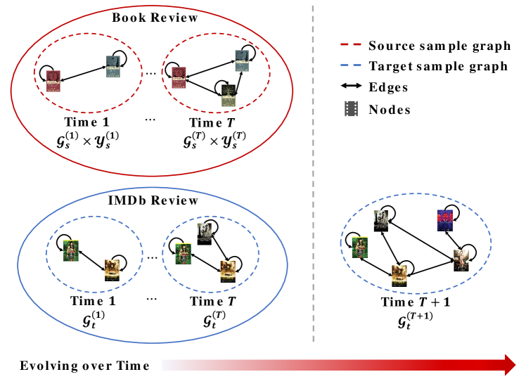
Figure 1. An illustrative example of dynamic transfer learning across book review network and IMDb review network. As an example, IMDb launched a new series in 2022, The Lord of the Rings: The Rings of Power, while the original book of this series has been published for decades. It is very natural to transfer knowledge from the information-rich source domain (book review network) to the information-scarce target domain (IMDb review network) across time in order to solve the target task (IMDb review prediction) at $\mathcal{G}_{t}^{(T+1)}$.

Transfer learning has a longstanding history (Tripuraneni et al., 2020; Wang et al., 2019; Ganin et al., 2016; Ben-David et al., 2010, 2006), which aims to improve the generalization performance of target domain leveraging knowledge from related source domain in another field. Graph-structured data poses unique challenges in knowledge transfer as graph signals (e.g., nodes, motifs, subgraphs) are naturally interconnected through edges and are not independent and identically distributed (i.i.d). Although it has been studied in a few recent works (Zhu et al., 2021; Hu et al., 2020; Wu et al., 2020; Shen et al., 2020), the vast majority of existing works do not take into account the dynamics of domains (Wu and He, 2022) in realistic networks. In Figure 1, we present a motivational example of dynamic transfer learning across book review network and IMDb review network. A naive solution would be directly employing the static graph-based transfer learning models on each timestamp, which might face two fundamental defects in practice. Firstly, learning from scratch at each timestamp would result in prohibitive computational costs, especially when data is collected from large-scale networks with a massive number of timestamps. Secondly, it fails to characterize domain evolution such that we can neither understand how and why changes in graphs occur at a specific time nor can we understand the impact on the generalization performance of the target domain in future timestamps.

We have identified three main challenges for filling the gap and alleviating the above issues of dynamic transfer learning across graphs. C1. Generalization Performance: There is no theoretical analysis on how the discrepancy would accumulate across time and whether it will further deteriorate performance, which hinders algorithmic design. Carrying out theoretical analysis on the generalization bound would be exciting for guiding future work of dynamic transfer learning across graphs. C2. Evolving Domain Discrepancy: How to disentangle the evolving domain discrepancy and capture the domain-invariant information when the source and target graphs exhibit distinct distributions of spatial, especially considering they change over time? C3. Benchmarks: How to identify the right benchmarks with features and structure of graphs evolving over time? As there is no existing literature on graph dynamic transfers, it is essential to point out a set of benchmark datasets and strong baselines for future algorithm development.

To the best of our knowledge, we are the first to define and study dynamic transfer learning across graphs. In this paper, we derive a tighter generalization error bound than existing results (Wu and He, 2022) to address C1. The theoretical findings illustrate that the generalization performance is dominated by historical empirical error and domain discrepancy. It also serves as theoretical support to our proposed DyTrans, which is a generic learning framework to enhance knowledge transfer across dynamic graphs. Our proposed approach consistently achieves outstanding performance on various backbones including classical GNNs, temporal GNNs, and transfer learning methods. In particular, to address C2, we utilize a Transformer module to model domain evolution. It obtains the temporal graph representation in evolving domain by using multi-head attention and generalizing positional encoding to the graph domain with temporal encoding. Moreover, we develop dual gradient reversal layers (GRLs) for minimizing domain discrepancy, which learn invariant representations to unify the source and target domains’ spatial and temporal information. To address C3, we extensively searched for existing temporal graphs and construct six pairs of datasets, which have rich dynamic properties regarding nodes, edges, node attributes, and labels. Our experiments validate that these selected datasets can be used for dynamic transfer learning across graphs. It serves as a benchmark that promotes fair comparisons and better replicability for algorithms in this problem setting for future dynamic transfer learning algorithms.

In general, our contributions are summarized as follows.

• 1

Problem Definition: We formalize the dynamic transfer learning problem across graphs and identify multiple unique challenges inspired by real-world applications.

• 2

Theorem: For the first time, we derive a tight generalization bound for dynamic transfer learning across graphs in terms of historical error for capturing domain evolution and domain discrepancy. This is a tighter bound as we use the minimum of the empirical errors instead of the average error and use a new distance funtion to measure domain discrepancy compared to (Wu and He, 2022).

• 3

Algorithm: Inspired by our generalization bound, we propose a novel method named DyTrans that (1) unifies the heterogeneous graph signals and dissipate feature spaces, and (2) captures the interdependence over time in evolving graphs. The generalization bound justifies that our proposed framework could effectively improve the generalization performance.

• 4

Evaluation: We identify six benchmark datasets for dynamic transfer learning across graphs. With that, we systematically evaluate the performance of DyTrans by comparing them with ten baseline models, which verifies the efficacy of DyTrans and corroborates our theoretical findings.

• 5

Reproducibility: We publish our data and code at https://anonymous.4open.science/r/DyTrans-82C4/.

The rest of our paper is organized as follows. In Section 2, we introduce the notations and problem definition. In Section 3, we present the details of our proposed framework DyTrans and then derive the generalization bound of dynamic transfer learning across graphs. Experimental results with discussion are reported in Section 4. We review the existing related literature in Section 5. Finally, we conclude this paper in Section 6.

2. Preliminary

In this section, we introduce the background that is pertinent to our work and give the formal problem definition. Table 1 summarizes the main notations used in this paper. We use regular letters to denote scalars (e.g. $\mu$), boldface lowercase letters to denote vectors (e.g. $\mathbf{v}$), and boldface uppercase letters to denote matrices (e.g. $\mathbf{X}$).

Table 1. Symbols and notations.

Symbol	Description
$\mathcal{G}_{s}^{(i)}$, $\mathcal{G}_{t}^{(i)}$	input source and target graphs at timestamp $i$.
$\mathcal{V}_{s}^{(i)}$, $\mathcal{V}_{t}^{(i)}$	the set of nodes in $\mathcal{G}_{s}^{(i)}$ and $\mathcal{G}_{t}^{(i)}$.
$\mathcal{E}_{s}^{(i)}$, $\mathcal{E}_{t}^{(i)}$	the set of edges in $\mathcal{G}_{s}^{(i)}$ and $\mathcal{G}_{t}^{(i)}$.
$\mathbf{X}_{s}^{(i)}$, $\mathbf{X}_{t}^{(i)}$	the node feature matrices of $\mathcal{G}_{s}^{(i)}$, $\mathcal{G}_{t}^{(i)}$.
$\mathcal{Y}_{s}^{(i)}$, $\tilde{\mathcal{Y}}_{t}^{(i)}$	the set of labels in $\mathcal{G}_{s}^{(i)}$ and $\mathcal{G}_{t}^{(i)}$.
$N_{s}^{(i)}$, $N_{t}^{(i)}$	the size of sample graph $\mathcal{G}_{s}^{(i)}$, $\mathcal{G}_{t}^{(i)}$.
$d_{s}$, $d_{t}$	feature dimensions of $\mathbf{X}_{s}^{(i)}$, $\mathbf{X}_{t}^{(i)}$, $\forall i$.
$T$	number of timestamps.
$h(\cdot)$	node classifier for downstream task.
$\tilde{\Re}$	Rademacher complexity.
$W_{p}$	Wasserstein-$p$ distance.

In the setting of dynamic transfer learning across graphs, we use subscript $s$ and subscript $t$ to represent source and target, and superscript $(i)$ represent the $i^{\text{th}}$ timestamp. We define spaces of graphs as graph distribution ($\mathbb{G}_{s}^{(i)}$ for source and $\mathbb{G}_{t}^{(i)}$ for target at timestamp $i$). The observed graph in source at timestamp $i$ is defined as a source sample graph $\mathcal{G}_{s}^{(i)}\sim\mathbb{G}_{s}^{(i)}$ (parallel definition of target sample graph $\mathcal{G}_{t}^{(i)}\sim\mathbb{G}_{t}^{(i)}$). $\mathcal{G}_{s}^{(i)}$ and $\mathcal{G}_{t}^{(i)}$ are defined in the form of triplets, i.e. $\mathcal{G}_{s}^{(i)}=(\mathcal{V}_{s}^{(i)},\mathcal{E}_{s}^{(i)},\mathbf{X}_{s}^{(i)})$ and $\mathcal{G}_{t}^{(i)}=(\mathcal{V}_{t}^{(i)},\mathcal{E}_{t}^{(i)},\mathbf{X}_{t}^{(i)})$, where $\mathcal{V}_{s}^{(i)}$ and $\mathcal{V}_{t}^{(i)}$ represent the set of nodes, $\mathcal{E}_{s}^{(i)}$ and $\mathcal{E}_{t}^{(i)}$ represent the set of edges, and $\mathbf{X}_{s}^{(i)}$ and $\mathbf{X}_{t}^{(i)}$ represent the node features in $\mathcal{G}_{s}^{(i)}$ and $\mathcal{G}_{t}^{(i)}$, respectively. $T$ is the total number of timestamps that can be observed in history. Furthermore, we define labels of source at $i^{th}$ timestamp as $\mathcal{Y}_{s}^{(i)}$ and few labels of target as $\tilde{\mathcal{Y}}_{t}^{(i)}$. We use domain $\mathcal{D}_{s}^{(i)}$ to represent data distribution over $\mathcal{G}_{s}^{(i)}\times\mathcal{Y}_{s}^{(i)}$ ($\mathcal{D}_{t}^{(i)}$ for the target similarly). Next, we briefly review graph representation learning and dynamic transfer learning.

Graph Representation Learning. The key idea of graph representation learning is to generate low-dimensional representations in the embedding space to capture graph features and structure. Typical graph learning tasks include node classification, link prediction, and graph classification. Let $\mathcal{G}=(\mathcal{V},\mathcal{E})$ be a graph, $\mathcal{V}$ and $\mathcal{E}$ are the sets of nodes and edges. Node classification, the task we focus on in this paper, learns a function $\mathbf{v}\rightarrow\mathbb{R}^{d},\mathbf{v}\in\mathcal{V}$ to map each node of a graph onto a semantically meaningful embedding of dimension $d$ such that $d\ll|\mathcal{V}|$ and make predictions on embedding space. Unlike standard classification tasks where data is assumed to be i.i.d, node classification task requires modeling the highly complex interconnection between nodes. Thus, many graph neural networks have been proposed to aggregate information based on local graph neighborhoods to generate efficient and accurate node representations and can be applied to both static and dynamic graphs (Kazemi et al., 2020).

Dynamic Transfer Learning. Here a domain $\mathcal{D}$ represents data distribution over an input feature space $\mathcal{X}$ and an output label space $\mathcal{Y}$. Labeling function is represented as $f(\cdot):\mathcal{X}\mapsto\mathcal{Y}$. Let $\{\mathcal{D}_{s}^{(i)}\}_{i=1}^{T}$ and $\{\mathcal{D}_{t}^{(i)}\}_{i=1}^{T}$ be the labeled dynamic source domains and unlabeled (or few labeled) dynamic target domains respectively, $f_{s}^{(i)}$ and $f_{t}^{(i)}$ be the task-specific labeling functions in the $i^{th}$ source and target domains, where $i$ indicates timestamp, and there is $T$ in total. Dynamic transfer learning aims to improve the learning of the target labeling function $f_{t}^{(T+1)}$ in $\mathcal{D}_{t}^{(T+1)}$ using the knowledge in historical source and target domains under the situation $\{\mathcal{D}_{s}^{(i)}\}_{i=1}^{T}\neq\{\mathcal{D}_{t}^{(i)}\}_{i=1}^{T}$. Let $\mathcal{H}$ be the hypothesis class on $\mathcal{X}$ where a hypothesis is a function $h:\mathcal{X}\rightarrow\mathcal{Y}$. The expected error of the hypothesis $h$ on the source domain $\mathcal{D}_{s}^{(i)}$ at timestamp $i$ is given by $\epsilon_{s}^{(i)}(h)=\mathbb{E}_{\mathbf{x}\sim\mathcal{D}_{s}^{(i)}}[\mathcal{L}(h(\mathbf{x}),f_{s}^{(i)}(\mathbf{x}))],\forall h\in\mathcal{H}$, where $\mathcal{L}(\cdot,\cdot)$ is some loss function. Its empirical estimate is defined as $\hat{\epsilon}_{s}^{(i)}(h)=\frac{1}{N_{s}^{(i)}}\sum_{\mathbf{x}\sim\mathcal{D}_{s}^{(i)}}[\mathcal{L}(h(\mathbf{x}),f_{s}^{(i)}(\mathbf{x}))]$. We use the parallel notations $\epsilon_{t}^{(i)}(h)$ and $\hat{\epsilon}_{t}^{(i)}(h)$ for the target domain. In (Wu and He, 2022), the expected errror on the newest target domain is derived as follows,

(1) $$\epsilon_{t}^{(T+1)}(h) \leq\frac{1}{2T}\sum_{i=1}^{T}\left(\hat{\epsilon}_{s}^{(i)}(h)+\hat{\epsilon}_{t}^{(i)}(h)\right)+\frac{T+2}{2}(\tilde{d}+\tilde{\lambda})$$

$$+\tilde{\Re}\left(\mathcal{H}_{\mathcal{L}}\right)+\frac{\mu}{T}\sqrt{\frac{\log\frac{1}{\delta}}{2\tilde{m}}}$$

where $\tilde{d}=\mu\cdot\max\left\{\max_{1\leq i\leq T-1}d_{MMD}\left(\mathcal{D}^{(i)}_{s},\mathcal{D}^{(i+1)}_{s}\right),\right.\\ \left.d_{MMD}\left(\mathcal{D}^{(1)}_{s},\mathcal{D}^{(1)}_{t}\right),\max_{1\leq i\leq T}d_{MMD}\left(\mathcal{D}^{(i)}_{t},\mathcal{D}^{(i+1)}_{t}\right)\right\}$, $d_{MMD}$ is the Maximum Mean Discrepancy, $\tilde{\lambda}=\mu\cdot\max\left\{\max_{1\leq i\leq T-1}\right.\\ \left.\lambda_{*}\left(\mathcal{D}^{(i)}_{s},\mathcal{D}^{(i+1)}_{s}\right),\lambda_{*}\left(\mathcal{D}^{(1)}_{s},\mathcal{D}^{(1)}_{t}\right),\max_{1\leq i\leq T}\lambda_{*}\left(\mathcal{D}^{(i)}_{t},\mathcal{D}^{(i+1)}_{t}\right)\right\}$ and $\lambda_{*}$ measures the difference of the labeling functions. $\mathcal{H}_{\mathcal{L}}=\{(\mathbf{X},y)\mapsto\mathcal{L}(h(\mathbf{X},y):h\in\mathcal{H}\}$, $\tilde{\Re}\left(\mathcal{H}_{\mathcal{L}}\right)$ is a Rademacher complexity and $\tilde{m}=\sum_{i=1}^{T}\left(N^{(i)}_{s}+N^{(i)}_{t}\right)$ is the total number of training examples from historical source and target domains. However, this bound is a loose bound that sums the errors in all timestamps without capturing domain evolution.

Problem definition. We consider transferring knowledge from a series of time-evolving source sample graphs $\{\mathcal{G}_{s}^{(i)}\}_{i=1}^{T}$ to a series of time-evolving target sample graphs $\{\mathcal{G}_{t}^{(i)}\}_{i=1}^{T}$. Figure 1 illustrates the knowledge transfer to the newest IMDb review network by leveraging historical IMDb and book review networks. Here, each node in a graph indicates an entity (user, movie, book), and the co-reviewer determines the edge between two nodes. Nodes, edges, and their attributes are evolving over time. The node label is the popularity of the movie (book) at that time and is also changing. As shown in Figure 1, there are several obstacles. In the IMDb and book review networks, we observe that not only the graphs (i.e., nodes and edges are added or removed) are changing over time, but also the learning tasks are changing over time (i.e., class-membership distributions are evolving). Moreover, many existing works demonstrate(Zhu et al., 2021) that the precondition of successful knowledge transfer lies in whether domains are related and share common information. Without loss of generality, we make the following three assumptions for our problem setting.

Assumption 1 (Graph evolution).

Nodes and edges on the graph $\mathcal{G}_{s}^{(i)}$ and $\mathcal{G}_{t}^{(i)}$ can be either added or removed over time. Meanwhile, the node attributes of source and target graphs change over time.

Assumption 2 (Task Evolution).

The class labels of the source domains are changed and are available at any timestamp, but they share the same label space.

Assumption 3 (Domain Relatedness).

The source and target domains are related at the initial timestamp $i=1$. Given the notations above, we formally define the problem as follows.

Problem 1.

Dynamic Transfer Learning across Graphs
Given: (i) a set of source sample graphs $\{\mathcal{G}_{s}^{(i)}=(\mathcal{V}_{s}^{(i)},\mathcal{E}_{s}^{(i)},\mathbf{X}_{s}^{(i)})\}_{i=1}^{T}$ with rich label information $\{\mathcal{Y}_{s}^{(i)}\}_{i=1}^{T}$, and (ii) a set of target sample graphs $\{\mathcal{G}_{t}^{(i)}=(\mathcal{V}_{t}^{(i)},\mathcal{E}_{t}^{(i)},\mathbf{X}_{t}^{(i)})\}_{i=1}^{T+1}$ with few label information $\{\tilde{\mathcal{Y}}_{t}^{(i)}\}_{i=1}^{T+1}$.
Find: Accurate predictions $\hat{\mathcal{Y}}_{t}^{(T+1)}$ of unlabeled examples in the target sample graph $\mathcal{G}_{t}^{(T+1)}$.

3. Model

In this section, we introduce our proposed framework DyTrans for dynamic transfer learning across graphs. The key idea lies in regularizing the underlying evolving domain discrepancy, which mainly stems from the distribution shift due to domain evolution and the inherent domain discrepancy between the source and target domains. In particular, we start with deriving a novel generalization bound of Problem 1, which is composed of historical empirical errors on the source and target domains, domain discrepancies across time on source and target, and Rademacher complexity of the hypothesis class. Inspired by the theoretical results, we then develop the overall learning paradigm of DyTrans and discuss the details of how to model domain evolution and how to unify dynamic graph distribution. Finally, we present an optimization algorithm with pseudo-code for DyTrans.

Figure 2. The proposed DyTrans framework.

3.1. Theoretical Analysis

Here we propose the very first generalization guarantee under the setting of dynamic transfer learning across graphs. Our most related work is Wu and He (Wu and He, 2022), where they give an error bound for dynamic transfer learning. However, their work is limited in the following aspects: (1) it is a loose bound since it simply accumulates the empirical errors across time and calculates the average; (2) it separately measures the difference of graphs and difference of labels by Maximum Mean Discrepancy (MMD)(Gretton et al., 2012).

To derive a better error bound, the improvements are mainly from the following two terms: (1) we reduce $\sum_{i=1}^{T}\left(\hat{\epsilon}_{s}^{(i)}(h)+\hat{\epsilon}_{t}^{(i)}(h)\right)$ to the minimum value of historical empirical errors on source and target to capture the domain evolution. It prevents the error bound from being impacted by some extreme value, e.g. a surprisingly bad performance on a specific timestamp. (2) Wasserstein distance accumulates abundant research on graphs (Peyré et al., 2019) and shows benefits on promising generalization bound and the gradient property for transfer learning (Shen et al., 2018). Therefore, we propose to use a dynamic Wasserstein distance (Villani, 2009) to replace $\tilde{d}$ for better measuring the evolving domain discrepancy.

Specifically, based on Lemma 1, we derive a generalization error bound with Wasserstein distance $W_{p}$ to measure the domain discrepancy. Next, based on Lemma 2, we give the expected error on the target domain at $N+1$ timestamp $\epsilon_{t}^{(T+1)}$, which is bounded by an expected error on an arbitrary domain. Thus, we can capture the domain evolution by the minimum of historical empirical errors on the source and target $\min_{1\leq i\leq T}\left(\hat{\epsilon}_{s}^{(i)}(h)+\hat{\epsilon}_{t}^{(i)}(h)\right)$. Following (Wang et al., 2022), Lemma 1 (Error Difference over Shifted Domains) states that the error difference on two arbitrary domains can be bounded by the measure of the domain discrepancy.

Lemma 0 (Error Difference over Shifted Domains (Wang et al., 2022)).

For arbitrary classifier $h$ and loss function $\mathcal{L}$ satisfying Assumption 4 and 5, the expected error of $h$ on two arbitrary domain $\mathcal{D}_{\mu}$ and $\mathcal{D}_{\nu}$ satisfies

(2) $$\left|\epsilon_{\mu}(h)-\epsilon_{\nu}(h)\right|\leq\rho\sqrt{R^{2}+1}W_{p}(\mathcal{D}_{\mu},\mathcal{D}_{\nu})$$

where $W_{p}$ is the Wasserstein-$p$ distance metric and $p\geq 1$.

Lemma 1 yields that the expected error on the target domain at $N+1$ timestamp $\epsilon_{t}^{(T+1)}$ is upper bounded with an expected error on an arbitrary domain and the maximum of measures of domain discrepancy. Then we consider the difference between the expected error and the empirical error on the arbitrary domain, it can be bounded using Lemma 2 (Algorithm Stability) following (Kumar et al., 2020).

Lemma 0 (Algorithm Stability (Kumar et al., 2020)).

Consider empirical and expected errors on arbitrary domain, $\forall~{}\delta\in(0,1)$, the following holds with probability at least $1-\delta$ for some constant $B>0$,

(3) $$\left|\hat{\epsilon}(h)-\epsilon(h)\right|\leq\mathcal{O}\left(\frac{\rho B+\sqrt{\log\frac{1}{\delta}}}{\sqrt{n}}\right)$$

From Lemma 2, we further bound $\epsilon_{t}^{(T+1)}$ with minimal empirical errors on the source and target and the maximum domain discrepancy. To summarize, according to historical source and target knowledge, the error of the latest target domain $\epsilon_{t}^{(T+1)}$ can be bounded, as stated by the following theorem 3.

Theorem 3.

Assume classifier $h$ is $R$-Lipschitz and loss function $\mathcal{L}(\cdot,\cdot)$ is $\rho$-Lipschitz. For any $\delta>0$ and $h\in\mathcal{H}$, with probability at least $1-\delta$, the error $\epsilon_{t}^{(T+1)}$ is bounded by:

(4) $$\epsilon_{t}^{(T+1)}(h) \leq\frac{1}{2}\min_{1\leq i\leq T}\left(\hat{\epsilon}_{s}^{(i)}(h)+\hat{\epsilon}_{t}^{(i)}(h)\right)+\frac{T^{2}+4T-2}{2T}\tilde{W_{p}}$$

$$+\tilde{\Re}\left(\mathcal{H}_{\mathcal{L}}\right)+\mathcal{O}\left(\frac{\rho B}{\sqrt{\tilde{n}}}+\sqrt{\frac{\log\frac{1}{\delta}}{\tilde{n}}}\right)$$

where $R$ and $\rho$ are the Lipschitz constants, dynamic Wasserstein distance $\tilde{W}_{p}=\rho\sqrt{R^{2}+1}\max\left(\max_{1\leq i\leq T-1}W_{p}(\mathcal{D}_{s}^{(i)},\mathcal{D}_{s}^{(i+1)}),\right.\\ \left.W_{p}(\mathcal{D}_{s}^{(1)},\mathcal{D}_{t}^{(1)}),\max_{1\leq i\leq T}W_{p}(\mathcal{D}_{t}^{(i)},\mathcal{D}_{t}^{(i+1)})\right)$, $W_{p}$ is Wasserstein-$p$ distance, $p\geq 1$, $\mathcal{H}_{\mathcal{L}}=\{(\mathbf{X},y)\mapsto\mathcal{L}(h(\mathbf{X},y):h\in\mathcal{H}\}$, $\tilde{\Re}(\mathcal{H}_{\mathcal{L}})=\frac{1}{2T}\sum_{i=1}^{T}\left(\tilde{\Re}_{\mathcal{D}_{s}^{(i)}}(\mathcal{H}_{\mathcal{L}})+\tilde{\Re}_{\mathcal{D}_{t}^{(i)}}(\mathcal{H}_{\mathcal{L}})\right)$, $\tilde{\Re}$ is Rademacher complexity, $B>0$ is a constant, and $\tilde{n}=\min_{1\leq i\leq T}\left(N_{s}^{(i)},N_{t}^{(i)}\right)$ is the minimal number of training examples in source and target domains.

Proof.

The detailed proof is provided in Appendix A. ∎

The theorem shows that the error on the latest target domain $\epsilon_{t}^{(T+1)}$ is bounded in terms of (1) the minimum value of empirical errors in the historical source and target domains; (2) the maximum of domain discrepancies across time and domain; (3) the average Rademacher complexity of hypothesis class over all domains.

Remarks: Compared to the existing theoretical results on dynamic transfer learning (Wu and He, 2022), we obtain a significantly improved bound in the following aspects.

• 1

Instead simply averaging the errors over time as (Wu and He, 2022), we propose to use the minimum of empirical errors over time to imply domain evolution and avoid extreme errors, which leads to a tighter bound.

$$\frac{1}{2}\min_{1\leq i\leq T}\left(\hat{\epsilon}_{s}^{(i)}(h)+\hat{\epsilon}_{t}^{(i)}(h)\right)<\frac{1}{2T}\sum_{1\leq i\leq T}\left(\hat{\epsilon}_{s}^{(i)}(h)+\hat{\epsilon}_{t}^{(i)}(h)\right)$$

• 2

Instead of separately measuring the difference of graphs and the difference of labels based on MMD, we propose a dynamic Wasserstein distance to model the evolving domain discrepancy.

In general, this tight bound guarantees the transferability from evolving source domains to evolving target domains and motivate us to propose a framework for dynamic transfer learning across graphs by empirically minimizing generalization bounds with domain evolution and domain discrepancy.

3.2. DyTrans Framework

According to the existing literature (Wu and He, 2022), a typical dynamic transfer learning paradigm can be formulated as follows.

(5) $$\min_{\theta}\mathcal{L}(\theta)=\sum_{i=1}^{T}\left(\hat{\epsilon}_{s}^{(i)}(\theta)+d(\mathcal{D}^{(i)}_{s},\mathcal{D}^{(i)}_{t},\theta)\right)$$

However, Eq. 5 may not well capture evolving domain discrepancy in practice due to the following two reasons. Frist, Eq. 5 simply sum up the empirical errors over time, which ignores the evolution process of dynamic graphs, i.e., the changes in the future snapshot $\mathcal{G}_{s}^{(t+1)}$ are often highly dependent to the structure of the current snapshot $\mathcal{G}_{s}^{(t)}$(Kazemi et al., 2020). Second, accumulating the domain discrepancy over all timestamps might lose track of the fine-grained information on how domain discrepancies change, e.g., the domain discrepancy $d(\mathcal{D}^{(T)}_{s},\mathcal{D}^{(T)}_{t},\theta)$ in the last timestamp could play a key role in the success of downstream task in the timestamp $T+1$.

Following our generalization bound, the generalization performance is dominated by two factors: the domain evolution across time and the domain discrepancy on source and target. Inspired by this, we proposed DyTrans (the overview is presented in Fig 2), which consists of two major modules: M1. Modeling domain evolution via temporal encoding and M2. Dynamic Graph Distribution Unification. These two modules are designed to address two types of discrepancy correspondingly. In particular, M1 introduces a temporal encoding for dynamic graphs, which encodes temporal information into the representation with continuous values and captures domain evolution by attention; M2 further unifies disparate spatial information of source and target into the domain-invariant hidden spaces. In addition, both M1 and M2 are absolutely necessary to overcome the main obstacles in dynamic transfer learning across graphs. M1 ensures accurate modeling of distribution shift due to domain evolution and characterizes historical temporal information for future downstream task-related representation learning, while M2 ensures extraction of domain-invariant spatial information that could be transferred to benefit the target domain. Our ablation study (Table  4) firmly attests both M1 and M2 are essential in a successful dynamic graph transfer. Next, we dive into the discussion of M1 and M2 in details.

M1. Modeling domain evolution via temporal encoding. For regularizing the distribution shift, it is essential to characterize the evolution of domains. Intuitively, the previous work (Wu and He, 2022) accumulate dynamic domain discrepancy over all timestamps using accumulative methods such as LSTM (Zhao et al., 2019; Taheri and Berger-Wolf, 2019). However, the new error bound provides a new interpretation: it may be more helpful to consider domain discrepancy uniformly across time and across domains. Therefore, we propose to characterize the dynamic domain discrepancy of certain time windows and view the time window for each domain as a whole by the transformer. Transformers have achieved supreme performance and computational efficiency in various tasks with sequential data by flexibly modeling dependencies between timestamps. In contrast, in recurrent models (Chung et al., 2014; Hochreiter and Schmidhuber, 1997), the next timestamp is factored based on previous timestamps. However, the positional encoding in classic Transformer models (Vaswani et al., 2017) only distinguishes the symbolic order of inputs instead of the continuous time values. For example, the positions of words in a sentence only indicate the order relationship and do not correspond to values with physical meaning that represent time. Meanwhile, the symbolic orders fail to retain multi-resolution timestamps, that is, the time gap between inputs may differ, and we hope to learn from this unequally distant gap. For example, as shown in Fig. 3, there are two levels of multi-resolution timestamps for the book review network and IMDb review network: (1) Multi-resolution timestamps across domains. Timestamps of book reviews may change by day as shown in (a), while the recording of movie reviews may be done in hours as shown in (b); (2) Multi-resolution timestamps within a domain, for different books in the book review network, timestamps for book ratings may also vary as shown in (a).

Figure 3. An illustrative example of why multi-resolution temporal encoding is important.

One key challenge in temporal modeling for dynamic graphs is that each input graph is associated with a timestamp that is continuous and often irregular and cannot be calculated arithmetically. In this work, we adopt multi-resolution temporal encoding (da Xu et al., 2020; Zhong and Huang, 2023) (capturing temporal information) to replace positional encoding (capturing sequential ordering) to solve this problem. We automatically encode temporal information into hidden representations with continuous values. Specifically, the multi-resolution temporal encoding is learned as:

(6) $$\texttt{ENC}=\sum_{i=1}^{T}\texttt{POSITION}(\texttt{CONTEXT}(\mathcal{G}^{(i)}_{s},\mathcal{G}^{(i)}_{t}))$$

where CONTEXT is the context extraction function (Starnini et al., 2012) that extracts temporal random walks from the input graphs, the POSITION is the positional encoding function (Dai et al., 2019) that considers node as a token, continuous-valued timestamp as a position to capture the multi-resolution temporal information. Notably, under the setting of dynamic transfer learning on the graph, the multi-resolution temporal encoding we used across the source and target domains.

Next, we introduce the attention layer to obtain important temporal graph representation for domain evolution. Notably, through previous operations in this framework, node embeddings of source and target sample graphs are converted into the same dimensionality. Therefore, a parameter-shared attention layer can be used for source and target domains to learn domain-invariant temporal node embeddings and also improve the model scalability because of its parallelism. Specifically, for each node, we group its temporal embeddings across all the timestamps and pack them into a matrix where the order is consistent with the corresponding timestamps. Notably, the number of timestamps in the source and target domain can be different since the cross-domain attention layer can handle inputs with variant lengths. Then this temporal-related matrix is respectively mapped into query $Q\in\mathbb{R}^{T\times d}$, key $K\in\mathbb{R}^{T\times d}$, and value $V\in\mathbb{R}^{T\times d}$ matrices (Vaswani et al., 2017). And the output of the attention layer indicates the relevance and importance of different timestamps for capturing domain evolution knowledge in terms of a specific node. We perform the same attention operation for all the nodes. Our cross-domain self-attention layer has advantages in two aspects: (1) by applying the attention layer on the source domain (target domain), we capture the information of the source domain (target domain) across time and thus can model $W_{p}(\mathcal{D}_{s}^{(i)},\mathcal{D}_{s}^{(i+1)})$ ($W_{p}(\mathcal{D}_{t}^{(i)},\mathcal{D}_{t}^{(i+1)})$) in the error bound; (2) by sharing the attention parameters of the source and target domains, we can capture $W_{p}(\mathcal{D}_{s}^{(1)},\mathcal{D}_{t}^{(1)})$ in the error bounds.

In this paper, we utilize multi-head attention (Vaswani et al., 2017) to capture information at different positions of the temporal input. Specifically, given an input matrix, multiple groups of different Q, K, and V are calculated by multiple heads respectively and are performed in parallel. Subsequently, the outputs of all these different heads are concatenated and re-projected for the follow-up process.

Through the Transformer module, we regularize the distribution shift, in which timestamps are represented as continuous values with temporal encoding, and temporal graph representations on the source and target domains are extracted with multi-head attention.

M2. Dynamic Graph Distribution Unification. To regularize the inherent domain discrepancy between source and target domains, we aim to learn domain-invariant representations and exclude discriminative information about the input (i.e., source sample graphs or target sample graphs). Gradient Reversal Layer (Ganin et al., 2016) connects representation extractor (i.e., GNN Layers or Transformer) with domain classifier (i.e., distinguishing source and target domains) to simultaneously generate representations that are domain-invariant for knowledge transfer and discriminative for domain classifier in an adversarial manner.

However, dual divergences (spatial and temporal divergences) are naturally provided when transferring knowledge from data in the form of graphs. As a result, we apply a dual GRLs module to learn domain-invariant spatial and temporal graph representations. First, we convert the size of feature dimensions from $d_{s},d_{t}$ to a fixed $d_{u}$ via multi-layer perceptrons (MLPs). Therefore, we can share the parameters of GNN for source and target sample graphs to better learn spatial information. We unified the MLP and the GNN into one unit named GNN Layers, and then one GRL is utilized on this unit to obtain the spatial invariant across domains. Similarly, we extract the temporal invariant using GRL after capturing domain evolution and obtaining temporal graph representations by the domain-invariant Transformer.

Gradient Reversal layer has no parameters and does not require parameter updates. It is implemented in the following simple steps: (1) During forward propagation, GRL acts as an identity. (2) While during back propagation, for the gradient from the next layer, GRL changes its sign via multiplying by $-1$ and then passes the changed gradient to the previous layer. The mathematical form of the loss function $\mathcal{L}_{GRL}$ of M2 can be expressed as follows:

(7) $$\mathcal{L}_{\text{GRL}} =Unif_{spatial}+Unif_{temporal}$$

$$=\sum_{i=1}^{T}\text{GRL}\left(\text{GNN}(\mathcal{G}_{s}^{(i)}),\text{GNN}(\mathcal{G}_{t}^{(i)})\right)$$

$$+\sum_{i=1}^{T}\text{GRL}\left(\text{Transformer}(\mathcal{G}_{s}^{(i)}),\text{Transformer}(\mathcal{G}_{t}^{(i)})\right)$$

where $Unif_{spatial}$ and $Unif_{temporal}$ represent the spatial divergence loss on GNN Layers and the temporal divergence loss on Transformer, respectively. In summary, M2 uses this dual GRLs to retain the domain-invariant information while excluding the domain-specific information.

3.3. Optimization

Overall, the goal of the training process is to minimize the domain classification loss in GRLs (for all sample graphs) and the node classification loss (for source sample graphs and few labeled nodes in target sample graphs). We define node classification loss as follows:

(8) $$\mathcal{L}_{task} =\mathcal{L}_{source}+\mathcal{L}_{target}$$

$$=\sum_{i=1}^{T}\mathcal{L}_{CE}\left(h(\mathcal{G}_{s}^{(i)}),\mathcal{Y}_{s}^{(i)}\right)+\gamma_{1}*\sum_{i=1}^{T+1}\mathcal{L}_{CE}\left(h(\tilde{\mathcal{G}}_{t}^{(i)}),\tilde{\mathcal{Y}}_{t}^{(i)}\right)$$

where $h(\cdot)$ is the classifier for the downstream task, $\mathcal{L}_{source}$ and $\mathcal{L}_{target}$ represent the node classification loss on the source and target domains, $\tilde{\mathcal{G}}_{t}^{(i)}\in\mathcal{G}_{t}^{(i)}$ represents limited labeled nodes in $\mathcal{D}_{t}^{(i)}$, and the contribution of the two terms is balanced by $\gamma_{1}$. Then the overall loss function can be written as follows:

(9) $$\mathcal{L}_{total}=\mathcal{L}_{\text{GRL}}+\gamma_{2}*\mathcal{L}_{task}$$

where $\mathcal{L}_{GRL}$ represents the dual GRLs loss, $\mathcal{L}_{task}$ represents the loss for classification on labeled nodes, and the hyperparameter $\gamma_{2}$ balances the contribution of the two terms. By minimizing these two losses, we control the domain evolution and domain discrepancy to improve the generalization performance.

Algorithm 1 The DyTrans Learning Framework.

0:    (i) a set of source sample graphs $\{\mathcal{G}_{s}^{(i)}=(\mathcal{V}_{s}^{(i)},\mathcal{E}_{s}^{(i)},\mathbf{X}_{s}^{(i)})\}_{i=1}^{T}$ with rich label information $\{\mathcal{Y}_{s}^{(i)}\}_{i=1}^{T}$; (ii) a set of target sample graphs $\{\mathcal{G}_{t}^{(i)}=(\mathcal{V}_{t}^{(i)},\mathcal{E}_{t}^{(i)},\mathbf{X}_{t}^{(i)})\}_{i=1}^{T+1}$ with few label information $\{\tilde{\mathcal{Y}}_{t}^{(i)}\}_{i=1}^{T+1}$.

0:    Prediction $\hat{\mathcal{Y}}_{t}^{(T+1)}$ of unlabeled examples in $\mathcal{G}_{t}^{(T+1)}$.

1:   Initialize two MLPs for source and target, the domain-invariant GNN, the domain-invariant Transformer, the dynamic graph distribution unification model, and the classifier $h(\cdot)$ for the downstream task in $\mathcal{G}_{t}^{(T+1)}$.

2:  while not converge do

3:      Compute representations in a shared latent space of both $\{\mathcal{G}_{s}^{(i)}\}_{i=1}^{T}$ and $\{\mathcal{G}_{t}^{(i)}\}_{i=1}^{T+1}$ via two MLPs.

4:      Compute domain-invariant spatial representations of both $\{\mathcal{G}_{s}^{(i)}\}_{i=1}^{T}$ and $\{\mathcal{G}_{t}^{(i)}\}_{i=1}^{T+1}$ via the domain-invariant GNN and first GRL.

5:      Compute domain-invariant temporal graph representations of both $\{\mathcal{G}_{s}^{(i)}\}_{i=1}^{T}$ and $\{\mathcal{G}_{t}^{(i)}\}_{i=1}^{T+1}$ via the domain-invariant Transformer and second GRL.

6:      Update the hidden parameters of two MLPs, the GNN, the Transformer, and the dynamic graph distribution unification model by minimizing the loss function in Eq. 9.

7:  end while

8:  while not converge do

9:     Fine-tune MLP for the target domain, the GNN, the Transformer, and the classifier $h(\cdot)$ for the downstream task.

10:  end while

The pseudo-code of DyTrans is provided in Algorithm 1, with Adam (Kingma and Ba, 2015) as the optimizer. Given a set of source sample graphs $\{\mathcal{G}_{s}^{(i)}=(\mathcal{V}_{s}^{(i)},\mathcal{E}_{s}^{(i)},\mathbf{X}_{s}^{(i)})\}_{i=1}^{T}$ with rich label information $\{\mathcal{Y}_{s}^{(i)}\}_{i=1}^{T}$, and a set of target graphs $\{\mathcal{G}_{t}^{(i)}=(\mathcal{V}_{t}^{(i)},\mathcal{E}_{t}^{(i)},\mathbf{X}_{t}^{(i)})\}_{i=1}^{T+1}$ with few label information $\{\tilde{\mathcal{Y}}_{t}^{(i)}\}_{i=1}^{T+1}$, our proposed DyTrans framework aims to predict $\hat{\mathcal{Y}}_{t}^{(T+1)}$ in the latest target sample graph $\mathcal{G}_{t}^{(T+1)}$. We initialize all the models and the classifier in Step 1. Steps 2-7 correspond to the pre-train process: in Step 3, we map sample graphs from source and target domains to a shared latent space using two separate MLPs; then the mapped representations are passed to a domain-invariant GNN for computing domain-invariant spatial representations in Step 4; followed by a domain-invariant Transformer for computing domain-invariant temporal graph representations in Step 5; while in Step 6, models are trained by minimizing the objective function. In Steps 8-10, we fine-tune the MLP of the target domain, the domain-invariant GNN, the domain-invariant Transformer, and the classifier $h(\cdot)$ on the latest target domain $\mathcal{G}_{t}^{(T+1)}$.

4. Experiments

In this section, we evaluate the performance of DyTrans on six benchmark datasets. DyTrans exhibits superior performances compared to various state-of-the-art baselines. We show the necessity of each ingredient of DyTrans in ablation studies. We also report the sensitivity analysis, which demonstrates DyTrans achieves a convincing performance with minimal tuning efforts.

4.1. Experiment Setup

Datasets: We evaluate DyTrans on our benchmark which is composed of three real-world graphs, including two graphs extracted from DBLP: DBLP-3 and DBLP-5 (Fan et al., 2021), where nodes represent authors, edges represent the co-authorship between two linked nodes; and one graph generated from functional magnetic resonance imaging (fMRI) data: Brain (Fan et al., 2021), where nodes represent cubes of brain tissue, edges represent that two linked cubes show similar degrees of activation. Each node of these three graphs is associated with one label only. Our benchmark follows these principles: (1) Dynamic: data follows the settings of (A1) graph evolution and (A2) task evolution in problem definition. (2) Transferability: there are existing works that have explored knowledge transfer across heterogeneous domains (Moon and Carbonell, 2017; Day and Khoshgoftaar, 2017). Therefore, data follows (A3) domain relatedness, and validity in dynamic transfer learning across graphs is proven by experiments. (3) Accessibility: data should be made available under a license that permits use and redistribution for research. The details of our benchmark are summarized in Table 2.

Table 2. Benchmark statistics.

Benchmark	Source	Target	Benchmark	Source	Target
1	DBLP-5	DBLP-3	4	Brain	DBLP-5
2	Brain	DBLP-3	5	DBLP-3	Brain
3	DBLP-3	DBLP-5	6	DBLP-5	Brain

Dataset	#Nodes	#Edges	#Attributes	#Classes	#Timestamps
DBLP-3	4,257	23,540	100	3	10
DBLP-5	6,606	42,815	100	5	10
Brain	5,000	1,955,488	20	10	12

Comparison Baselines: We compare DyTrans with four classical graph neural networks, four temporal graph neural networks and two graph transfer learning methods.

• 1

Classical GNNs: GCN (Kipf and Welling, 2017), GAT (Veličković et al., 2018), GIN (Xu et al., 2019), GraphSAGE (Hamilton et al., 2017) are four standard graph representation benchmark architectures.

• 2

Temporal GNNs: DCRNN (Li et al., 2017) captures both spatial and temporal dependencies of graphs among time series. DyGrEncoder (Taheri and Berger-Wolf, 2019) models embedding GNN to LSTM. EvolveGCN (Pareja et al., 2020) uses a GCN evolved by an RNN to capture the dynamism of graph sequence. TGCN (Zhao et al., 2019) is a combination of GCN and the gated recurrent unit.

• 3

Transfer Learning Methods: DANN (Ganin et al., 2016) is the first method using GRL for domain adaptation. UDAGCN (Wu et al., 2020) is a method for domain adaptation in the static graph using attention mechanism.

Implementation Details: For a fair comparison, the output dimensions of all GNNs including baselines and DyTrans are set to 16. We conduct experiments with only five labeled samples in each class of the target dataset and test model performance based on all the rest unlabeled nodes. For non-temporal GNNs, since they cannot process dynamic graphs directly, we train each model on the graph of the last timestamp. Specifically, for classical GNNs, they are trained on the target dataset for 1000 epochs; for transfer learning models, after training on the source dataset for 2000 epochs, they are fine-tuned on the target dataset for 600 epochs. We use GCN as the feature extractor of DANN, and follow the instruction from the original paper of UDAGCN (Wu et al., 2020) to build a union set for input features between the source and target domains by setting zeros for unshared features. For four temporal GNNs, they are trained using all timestamps of the target dataset for 1000 epochs.

For DyTrans, it is firstly pre-trained for 2000 epochs, then fine-tuned on the target dataset for 600 epochs using limited labeled data in each class. Since the label of each node in current benchmarks is consistent in every timestamp, in this paper, the output of the Transformer in DyTrans is aggregated using average along all the timestamps; but our model can easily be applied to the settings where labels of each node are changed in different timestamps by simply removing the aggregation operation. We use Adam optimizer with learning rate 3e-3. Considering the imbalanced label distribution, the area under the receiver of characteristic curve (AUC) is used as the evaluation metric. We run all the experiments with 25 random seeds. The experiments are performed on a Ubuntu20 machine with 16 3.8GHz AMD Cores and a single 24GB NVIDIA GeForce RTX3090.

4.2. Effectiveness

4.2.1. Comparison Results.

We compare DyTrans with ten baseline methods across three real-world undirected graphs. We report the AUC of different methods on the last timestamp of the target domain in Table 3. In general, we have the following observations: (1) DyTrans consistently outperforms all ten baselines on all the datasets, which demonstrates the effectiveness and generalizability of our model. Especially, when adapting knowledge from DBLP-5 to DBLP-3 with five labeled samples per class, the improvement is 7% comparing with the second best model (EvolveGCN). (2) Classical GNNs have the worst performance on four benchmarks (1, 2, 3, 4) since they neither can learn knowledge from the previous timestamps, nor transfer knowledge from other domains. DyTrans boosts the performance compared with classical GNNs by up to 10.8% (on benchmark 6). (3) Temporal GNNs achieve the second best performance on Benchmark 1 and 2, which means in these benchmarks, there are knowledge existing in the previous timestamps that is useful for the label prediction task in the future timestamps. Particularly, DyTrans still outperforms these temporal GNNs on Benchmark 1 and 2 by up to 8%. Notably, on Benchmark 5 and 6, all temporal GNNs fail, while DyTrans can still has the best performance. (4) Transfer learning models have the second best performance on Benchmark 5 and 6, which shows the efficacy of the domain knowledge transfer on these two benchmarks. Especially, DyTrans still does better than this kind of models on Benchmark 5 and 6 by up to 7.2% AUC.

	Classical GNNs				Temporal GNNs				Transfer learning		Ours
	GCN	GAT	GIN	GraphSAGE	DCRNN	DyGrEncoder	EvolveGCN	TGCN	DANN	UDAGCN	DyTrans
Benchmark 1	0.5609	0.5489	0.5454	0.5452	0.5637	0.5672	0.5823	0.5640	0.5416	0.5688	0.6527
Benchmark 2									0.5400	0.5523	0.6103
Benchmark 3	0.5404	0.5387	0.5422	0.5390	0.5518	0.5489	0.5610	0.5482	0.5395	0.5660	0.5915
Benchmark 4									0.5348	0.5651	0.5769
Benchmark 5	0.6756	0.6964	0.6962	0.6798	0.5710	0.6363	0.5679	0.5695	0.6977	0.7407	0.7975
Benchmark 6									0.6981	0.7320	0.8046

Table 3. Comparison of different methods in node classification task using 5 labeled samples per class (AUC). The first four models are Classical GNN models and the next four are Temporal GNNs, we show their fine-tuned results on the target domain. The remaining two models are for transfer learning, we show results of knowledge transfer from source to target domain.

4.2.2. Ablation Study

Considering that DyTrans consists of various components, we set up the following experiments to study the effect of different components by removing one component from DyTrans at a time: (1) removing the pre-training process; (2) removing the Transformer; (3) removing the domain losses (including $Unif_{spatial}$ and $Unif_{temporal}$). Due to the space limit, we use Benchmark 1, 5, and 6 to illustrate in this section. The ablation results are presented in Table 4. From the results, we have several interesting observations. (1) Pre-training can significantly boost the model performance by up to 8% (on Benchmark 6), which indicates the efficacy of knowledge transferring of our model across different graphs under the limited label setting. (2) Transformer achieves impressive improvement on Benchmark 5 and 6 by up to 7%, which shows its strength in temporal transfer learning and also supports our theoretical analysis in section 3.1. (3) Both two domain losses help the model better adapt knowledge from the source to the target domain. especially on Benchmark 1, the removal of $Unif_{spatial}$ ($Unif_{temporal}$) leads to a decrease in AUC by 1.6% (1.8%), p-value ¡ 0.001. This proves the effectiveness of dual GRLs module in alleviating the spatial and temporal discrepancies. (4) The improvements of M2 are not obvious in Benchmarks 5 and 6, and a simple guess is DyTrans variation with only M1 already achieves significant improvement than our baselines, so M2 makes less contribution to the final results.

Ablation	Benchmark 1	Benchmark 5	Benchmark 6
w/o pre-training	$0.5907\pm 0.70\%$	$0.7661\pm 1.32\%$	$0.7234\pm 1.49\%$
w/o Transformer	$0.6487\pm 2.09\%$	$0.7682\pm 1.05\%$	$0.7303\pm 1.97\%$
w/o $Unif_{spatial}$	$0.6367\pm 1.77\%$	$0.7939\pm 0.85\%$	$0.7985\pm 0.82\%$
w/o $Unif_{temporal}$	$0.6341\pm 1.50\%$	$0.7966\pm 0.87\%$	$0.8021\pm 0.63\%$
DyTrans	$\textbf{0.6527}\pm 1.86\%$	$\textbf{0.7975}\pm 0.78\%$	$\textbf{0.8046}\pm 0.67\%$

Table 4. Ablation study (AUC $\pm$ 95% confidence intervals).

4.3. Parameter Sensitivity Analysis

In this section, we study two hyper-parameters of our model: (1) the size of head dimension of the Transformer $d$; (2) the size of the mapped features $d_{u}$ of two MLPs in M2 (Dynamic Graph Distribution Unification module). The result is shown in Fig 4. Based on that, the fluctuation of the AUC (z-axis) is less than 3%. The AUC is slightly lower when the head dimension of the Transformer becomes larger, and different values of $d$ do not affect the AUC significantly. Overall, we find DyTrans is reliable and not sensitive to the hyperparameters under study within a wide range.

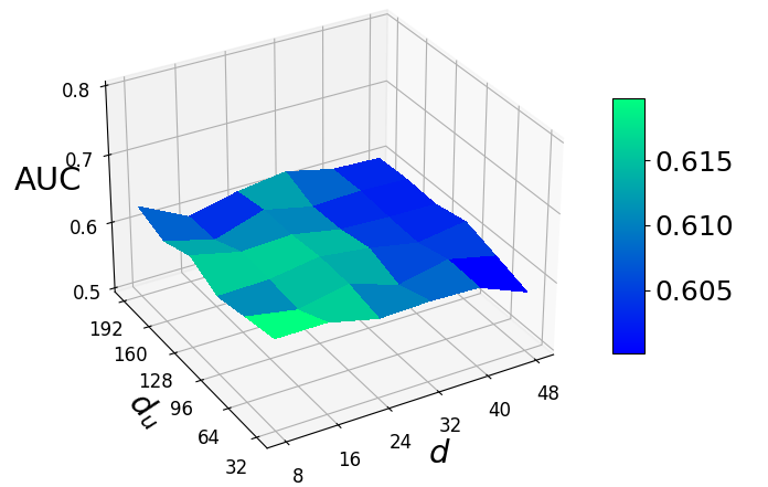
Figure 4. Hyper-parameter analysis on Benchmark 2 with respect to $d_{u}$ and $d$.

5. Related Work

In this section, we briefly review the existing literature in the context of dynamic transfer learning and graph neural networks.

Dynamic Transfer. Transfer learning aims to improve performance on target data by extracting and transferring knowledge from related but different source data (Pan and Yang, 2010; Zhuang et al., 2021). It has been revealed to be an efficient method to reduce the dependence on a large number of target data. It is commonly found in real-world applications due to the difficulty and time-consuming of obtaining labels and collecting data. Transfer learning has exhibited excellent performance in several areas, such as natural language processing (Yang et al., 2021; Ruder et al., 2019), computer vision (Zhang et al., 2022; Alhashim and Wonka, 2018), time series analysis (Bethge et al., 2022; Ismail Fawaz et al., 2018), and healthcare (Panagopoulos et al., 2021). Then, several works named “continuous transfer (Wang et al., 2021, 2020a; Desai et al., 2020)” or “dynamic domain adaptation (Li et al., 2021; Ke et al., 2021; Mancini et al., 2019)” are proposed to learn the evolving data. For example, Minku (Minku, 2019) manually partitioned source data into several evolving parts and manage to solve the non-stationary source domain by performing transfer learning. There are also some works (Hoffman et al., 2014; Ortiz-Jiménez et al., 2019; Liu et al., 2020; Wu and He, 2020; Wang et al., 2020b; Kumar et al., 2020; Xie et al., 2021) that addressed the scenario in which the source domain is static, and the target domain is continually evolving. Recently, Wu and He (Wu and He, 2022) modeled the knowledge transferability with dynamic source domain and dynamic target domain and defined this problem as “Dynamic Transfer Learning.” Despite the success of dynamic transfer learning, no effort has been made to solve the problem on graph-structured data. In this paper, we aim to explore the knowledge transferability on graphs.

Graph Neural Networks. Graph neural networks capture the structure of graphs via message passing between nodes. Many significant efforts such as GCN (Kipf and Welling, 2017), GraphSAGE (Hamilton et al., 2017), GAT (Veličković et al., 2018), GIN (Xu et al., 2019) arose and have become indispensable baseline in a wide range of downstream tasks. Here we do not intend to provide a comprehensive survey of the wide range of GNNs. Instead, we refer the reader to excellent recent surveys to get more familiar with the topics (Wu et al., 2021; Zhou et al., 2020). Recently, several attempts have been focused on generalizing GNN from static graphs to dynamic graphs (Skarding et al., 2021; Yu et al., 2018; Schlichtkrull et al., 2018; Kim et al., 2022; You et al., 2022). They fall into two categories according to graph types: (1) A dynamic graph is presented in the form of a set of static graph snapshots at certain timestamps. Under this setting, Pareja et al. (Pareja et al., 2020) first utilize common GCNs to learn node representations on each static graph snapshot and then aggregate these representations from the temporal dimension. (2) A temporal graph is given in the form of a start graph and a set of graph evolution with the corresponding timestamp. To solve this problem, Xu et al. (da Xu et al., 2020) first propose to use time embedding and design a temporal graph attention layer to concatenate node, edge, and time features efficiently. Kumar (Kumar et al., 2019) uses RNN to maintain and update node embeddings. However, the Dynamic GNN strategies often lack the capability of transferring knowledge, thus limiting their ability to leverage valuable information from other data sources. Here we further extend it to the transfer learning setting with dynamic source and target domains.

6. Conclusion

In this paper, we investigate a novel problem named dynamic transfer learning across graphs, which intends to augment knowledge transfer from dynamic source graphs to dynamic target graphs. We shed light on C1 (Generalization performance) by proposing a new generalized bound in terms of historical empirical error and domain discrepancy. We also present DyTrans, an end-to-end framework with two major modules: M1. Modeling domain evolution via temporal encoding and M2. Dynamic Graph Distribution Unification to alleviate evolving domain discrepancy that is specified in C2 (Evolving domain discrepancy). Extensive experiments on our carefully prepared benchmark, where DyTrans consistently outperforms state-of-art baselines, demonstrate the efficacy of our model for dynamic transfer learning across graphs.

Reproducibility: We have released our code and data at https://anonymous.4open.science/r/DyTrans-82C4/.

Appendix A Algorithm Analysis

First, for the classifier and loss function, we have the following assumptions.

Assumption 4 ($R$-Lipschitz Classifier (Wang et al., 2022)).

Assume each classifier $h\in\mathcal{H}$ is $R$-Lipschitz in $\ell_{2}$ norm, i.e., $\forall x,x^{\prime}\in\mathcal{X}$,

$$\left|h(x)-h\left(x^{\prime}\right)\right|\leq R\left\|x-x^{\prime}\right\|_{2}$$

Assumption 5 ($\rho$-Lipschitz Loss (Wang et al., 2022)).

Assume the loss function $\mathcal{L}(\cdot,\cdot)$ is $\rho$-Lipschitz if $\exists~{}\rho>0$ such that $\forall\mathbf{x}\in\mathcal{X}$, $y,y^{\prime}\in\mathcal{Y}$ and $h,h^{\prime}\in\mathcal{H}$, the following inequalities hold.

$$\left|\mathcal{L}\left(h^{\prime}(\mathbf{x}),y\right)-\mathcal{L}(h(\mathbf{x}),y)\right| \leq\rho\left|h^{\prime}(\mathbf{x})-h(\mathbf{x})\right|$$

$$\left|\mathcal{L}\left(h(\mathbf{x}),y^{\prime}\right)-\mathcal{L}(h(\mathbf{x}),y)\right| \leq\rho\left|y^{\prime}-y\right|$$

Next, we give the definition of Wasserstein distance between domains and Rademacher Complexity of hypothesis class.

Definition 0 ($p$-Wasserstein Distance (Villani, 2009)).

Consider two domains $\mathcal{D}_{\mu}$ and $\mathcal{D}_{\nu}$. For any $p\geq 1$, their $p$-Wasserstein distance metric is defined as:

(10) $$W_{p}(\mathcal{D}_{\mu},\mathcal{D}_{\nu})=\left(\inf_{\gamma\in\Gamma(\mathcal{D}_{\mu},\mathcal{D}_{\nu})}\int d(x,y)^{p}\mathrm{~{}d}\gamma(x,y)\right)^{1/p}$$

where $\Gamma(\mathcal{D}_{\mu},\mathcal{D}_{\nu})$ is the set of all measures over $\mathcal{D}_{\mu}\times\mathcal{D}_{\nu}$.

Definition 0 (Rademacher Complexity (Bartlett and Mendelson, 2002)).

Given a sample $S=(\mathbf{X}_{1},\cdots,\mathbf{X}_{N})\in\mathcal{X}^{N}$, the empirical Rademacher complexity of $\mathcal{H}$ given $S$ is defined as:

(11) $$\hat{\Re}_{S}(\mathcal{H})=\mathbb{E}_{\bm{\sigma}}\left[\sup_{h\in\mathcal{H}}\sum_{i=1}^{N}\sigma_{i}h\left(\mathbf{x}_{i}\right)\mid S=\left(\mathbf{x}_{1},\cdots,\mathbf{x}_{N}\right)\right]$$

where $\bm{\sigma}=\left(\sigma_{1},\cdots,\sigma_{m}\right)$ is a vector of independent random variables from the Rademacher distribution.

Then, we use Lemma 1 to bound the error difference between arbitrary two domains and use Lemma 2 to bound the difference between empirical and expected errors. See 1

See 2

Lemma 0 (McDiarmid’s inequality).

Let function $f$ satisfies for all $1\leq i\leq N$, and all $\mathbf{X}_{1},\cdots,\mathbf{X}_{N},\mathbf{X}_{i}^{\prime}\in\mathcal{X}$ ,

(12) $$\left|f\left(\mathbf{X}_{1},\cdots,\mathbf{X}_{i},\cdots,\mathbf{X}_{N}\right)-f\left(\mathbf{X}_{1},\cdots,\mathbf{X}_{i}^{\prime},\cdots,\mathbf{X}_{N}\right)\right|\leq c_{i}$$

where bound $c_{1},\cdots,c_{N}$ are constants. Then, for any $\epsilon>0$,

(13) $$\operatorname{Pr}[f-\mathbb{E}[f]\geq\epsilon]\leq\exp\left(\frac{-2\epsilon^{2}}{\sum_{i=1}^{N}c_{i}^{2}}\right)$$

Based on the above conclusion, Theorem 3 and its proof are given as follows. See 3

Proof.

Let $\mathcal{D}_{s}^{(i)}$ and $\mathcal{D}_{t}^{(i)}$ be the source domain and the target domain at $i^{th}$ timestamp. $\mathcal{B}\in(\mathcal{G}\times\mathcal{Y})^{\tilde{n}}$ is the measurable subset over $\mathcal{D}_{s}^{(1)}\times\cdots\times\mathcal{D}_{s}^{(T)}\times\mathcal{D}_{s}^{(1)}\times\cdots\times\mathcal{D}_{t}^{(T)}$, and we define a function $g$ over $\mathcal{B}$ as follows (Wu and He, 2022).

(14) $$g(\mathcal{B})=\sup_{h\in\mathcal{H}}\epsilon_{t}^{(T+1)}(h)-\frac{1}{2T}\sum_{i=1}^{T}\left(\hat{\epsilon}_{s}^{(i)}(h)+\hat{\epsilon}_{t}^{(i)}(h)\right)$$

where $\hat{\epsilon}_{s}^{(i)}(h)$ and $\hat{\epsilon}_{t}^{(i)}(h)$ are the estimate errors on graph $\mathcal{G}_{s}^{(i)}$ and $\mathcal{G}_{t}^{(i)}$. Let $\mathcal{B}$ and $\mathcal{B}^{\prime}$ be two measurable subsets containing only one different source sample in $\mathcal{G}_{s}^{(i)}$, then we have

(15) $$\left|g(\mathcal{B})-g\left(\mathcal{B}^{\prime}\right)\right|\leq\frac{2\rho}{2N_{t}^{(i)}T}\leq\frac{\rho}{\tilde{n}T}$$

The same result holds for different target sample. Based on McDiarmid’s inequality (see Lemma 3), we have for any $\epsilon>0$

(16) $$\operatorname{Pr}\left[g(\mathcal{B})-\mathbb{E}_{\mathcal{B}}[g(\mathcal{B})]\geq\epsilon\right]\leq\exp\left(\frac{-2\tilde{n}T^{2}\epsilon^{2}}{\rho^{2}}\right)$$

Then, for any $\delta>0$, with probability at least $1-\delta$, the following holds

(17) $$g(\mathcal{B})\leq\mathbb{E}_{\mathcal{B}}[g(\mathcal{B})]+\frac{\rho}{T}\sqrt{\frac{\log\frac{1}{\delta}}{2\tilde{n}}}$$

In addition, for any $h\in\mathcal{H}$ and any $i\in\{1,\cdots,T\}$, we have

(18) $$\epsilon_{t}^{(i)}(h) =\epsilon_{s}^{(i)}(h)+\epsilon_{t}^{(i)}(h)-\epsilon_{s}^{(i)}(h)$$

$$(lemma~{}\ref{lemma:shift domains}) \leq\epsilon_{s}^{(i)}+\rho\sqrt{R^{2}+1}W_{p}(\mathcal{D}_{t}^{(i)},\mathcal{D}_{s}^{(i)})$$

Then, we have

(19) $$\sum_{i=1}^{T}\left(\epsilon_{t}^{(T+1)}(h)-\epsilon_{t}^{(i)}(h)\right)$$

$$= \epsilon_{t}^{(T+1)}(h)-\epsilon_{t}^{(T)}(h)+\cdots+\epsilon_{t}^{(2)}(h)-\epsilon_{t}^{(1)}(h)+\sum_{i=2}^{T}\left(\epsilon_{t}^{(T+1)}(h)-\epsilon_{t}^{(i)}(h)\right)$$

$$\leq \rho\sqrt{R^{2}+1}\left(W_{p}(\mathcal{D}_{t}^{(T)},\mathcal{D}_{t}^{(T+1)})+\cdots+W_{p}(\mathcal{D}_{t}^{(1)},\mathcal{D}_{t}^{(2)})\right)$$

$$+ \sum_{i=2}^{T}\left(\epsilon_{t}^{(T+1)}(h)-\epsilon_{t}^{(i)}(h)\right)$$

$$\leq T\tilde{W}_{p}+\sum_{i=2}^{T}\left(\epsilon_{t}^{(T+1)}(h)-\epsilon_{t}^{(i)}(h)\right)\leq\frac{T(T+1)}{2}\tilde{W}_{p}$$

Then

(20) $$\mathbb{E}_{\mathcal{B}}[g(\mathcal{B})]$$

$$= \mathbb{E}_{\mathcal{B}}\left[\sup_{h\in\mathcal{H}}\epsilon_{t}^{(T+1)}(h)-\frac{1}{2T}\sum_{i=1}^{T}\left(\hat{\epsilon}_{s}^{(i)}(h)+\hat{\epsilon}_{t}^{(i)}(h)\right)\right]$$

$$= \mathbb{E}_{\mathcal{B}}\left[\sup_{h\in\mathcal{H}}\epsilon_{t}^{(T+1)}(h)-\frac{1}{2T}\sum_{i=1}^{T}\left(\epsilon_{s}^{(i)}(h)+\epsilon_{t}^{(i)}(h)\right)\right.$$

$$\left.+\frac{1}{2T}\sum_{i=1}^{T}\left(\epsilon_{s}^{(i)}(h)-\hat{\epsilon}_{s}^{(i)}(h)\right)+\frac{1}{2T}\sum_{i=1}^{T}\left(\epsilon_{t}^{(i)}(h)-\hat{\epsilon}_{t}^{(i)}(h)\right)\right]$$

$$= \frac{1}{2T}\sup_{h\in\mathcal{H}}\left(\sum_{i=1}^{T}\left(\epsilon_{t}^{(T+1)}(h)-\epsilon_{t}^{(i)}(h)\right)+\sum_{i=1}^{T}\left(\epsilon_{t}^{(T+1)}(h)-\epsilon_{s}^{(i)}(h)\right)\right)$$

$$+\mathbb{E}_{\mathcal{B}}\left[\sup_{h\in\mathcal{H}}\frac{1}{2T}\sum_{i=1}^{T}\left(\epsilon_{s}^{(i)}(h)-\hat{\epsilon}_{s}^{(i)}(h)\right)+\frac{1}{2T}\sum_{i=1}^{T}\left(\epsilon_{t}^{(i)}(h)-\hat{\epsilon}_{t}^{(i)}(h)\right)\right]$$

$$\leq \frac{1}{2T}\sup_{h\in\mathcal{H}}\left(\sum_{i=1}^{T}\left(\epsilon_{t}^{(T+1)}(h)-\epsilon_{t}^{(i)}(h)\right)+\sum_{i=1}^{T}\left(\epsilon^{(1)}_{s}(h)-\epsilon_{s}^{(i)}(h)\right)\right.$$

$$\left.+\sum_{i=1}^{T}\left(\epsilon_{t}^{(T+1)}(h)-\epsilon^{(1)}_{t}(h)\right)+\sum_{i=1}^{T}\left(\epsilon^{(1)}_{t}(h)-\epsilon^{(1)}_{s}(h)\right)\right)$$

$$+\mathbb{E}_{\mathcal{B}}\left[\frac{1}{2T}\sum_{i=1}^{T}\sup_{h\in\mathcal{H}}\left(\epsilon_{s}^{(i)}(h)-\hat{\epsilon}_{s}^{(i)}(h)\right)+\frac{1}{2T}\sum_{i=1}^{T}\sup_{h\in\mathcal{H}}\left(\epsilon_{t}^{(i)}(h)-\hat{\epsilon}_{t}^{(i)}(h)\right)\right]$$

$$\leq \frac{1}{2T}\left[\frac{T(T+1)}{2}\tilde{W}_{p}+\frac{T(T-1)}{2}\tilde{W}_{p}+T\tilde{W}_{p}+T\tilde{W}_{p}\right]$$

$$+ \mathbb{E}_{\mathcal{B}}\left[\frac{1}{2T}\sum_{i=1}^{T}\tilde{\Re}_{\mathcal{D}_{s}^{(i)}}(\mathcal{H}_{\mathcal{L}})+\frac{1}{2T}\sum_{i=1}^{T}\tilde{\Re}_{\mathcal{D}_{t}^{(i)}}(\mathcal{H}_{\mathcal{L}})\right]$$

$$\leq \frac{T+2}{2}\tilde{W}_{p}+\tilde{\Re}(\mathcal{H}_{\mathcal{L}})$$

According to (14), we have for any $h\in\mathcal{H}$,

(21) $$\small\epsilon_{t}^{(T+1)}(h)\leq\frac{1}{2T}\sum_{i=1}^{T}\left(\hat{\epsilon}_{s}^{(i)}(h)+\hat{\epsilon}_{t}^{(i)}(h)\right)+\mathbb{E}_{\mathcal{B}}[g(\mathcal{B})]+\frac{\rho}{T}\sqrt{\frac{\log\frac{1}{\delta}}{2\tilde{n}}}$$

w.l.o.g., we assume $\hat{\epsilon}_{s}^{(1)}\leq\hat{\epsilon}_{s}^{(2)}\leq\cdots\leq\hat{\epsilon}_{s}^{(T)}$ for simplify, consider the last term in $\sum_{i=1}^{T}\left(\hat{\epsilon}_{s}^{(i)}(h)\right)$, for some constant $B>0$

$$(Proposition~{}\ref{lemma:stability})\hat{\epsilon}_{s}^{(T)}\leq \epsilon_{s}^{(T)}+\mathcal{O}\left(\frac{\rho B}{\sqrt{\tilde{n}}}+\sqrt{\frac{\log\frac{1}{\delta}}{\tilde{n}}}\right)$$

$$(lemma~{}\ref{lemma:shift domains})\leq \epsilon_{s}^{(T-1)}+\rho\sqrt{R^{2}+1}W_{p}(\mathcal{D}_{s}^{(T)},\mathcal{D}_{s}^{(T-1)})$$

(22) $$+ \mathcal{O}\left(\frac{\rho B}{\sqrt{\tilde{n}}}+\sqrt{\frac{\log\frac{1}{\delta}}{\tilde{n}}}\right)$$

$$\leq \cdots$$

$$\leq \epsilon_{s}^{(1)}+(T-1)\tilde{W}_{p}+\mathcal{O}\left(\frac{\rho B}{\sqrt{\tilde{n}}}+\sqrt{\frac{\log\frac{1}{\delta}}{\tilde{n}}}\right)$$

$$(Proposition~{}\ref{lemma:stability})\leq \hat{\epsilon}_{s}^{(1)}+(T-1)\tilde{W}_{p}+\mathcal{O}\left(\frac{\rho B}{\sqrt{\tilde{n}}}+\sqrt{\frac{\log\frac{1}{\delta}}{\tilde{n}}}\right)$$

for the second last term in $\sum_{i=1}^{T}\left(\hat{\epsilon}_{s}^{(i)}(h)\right)$, we have

(23) $$(Proposition~{}\ref{lemma:stability})\hat{\epsilon}_{s}^{(T-1)}\leq \epsilon_{s}^{(T-1)}+\mathcal{O}\left(\frac{\rho B}{\sqrt{\tilde{n}}}+\sqrt{\frac{\log(1/\delta)}{\tilde{n}}}\right)$$

$$\leq \epsilon_{s}^{(T)}+\mathcal{O}\left(\frac{\rho B}{\sqrt{\tilde{n}}}+\sqrt{\frac{\log\frac{1}{\delta}}{\tilde{n}}}\right)$$

$$(\ref{equ:lastTerm})\leq \hat{\epsilon}_{s}^{(1)}+(T-1)\tilde{W}_{p}+\mathcal{O}\left(\frac{\rho B}{\sqrt{\tilde{n}}}+\sqrt{\frac{\log\frac{1}{\delta}}{\tilde{n}}}\right)$$

It is easy to see that this can be bounded for source or target across time. Generally,

(24) $$\frac{1}{2T}\sum_{i=1}^{T}\left(\hat{\epsilon}_{s}^{(i)}(h)\right)\leq\frac{1}{2}\min_{1\leq i\leq T}(\hat{\epsilon}_{s}^{(i)})+\frac{T-1}{2T}\tilde{W}_{p}+\mathcal{O}\left(\frac{\rho B}{\sqrt{\tilde{n}}}+\sqrt{\frac{\log\frac{1}{\delta}}{\tilde{n}}}\right)$$

$$\frac{1}{2T}\sum_{i=1}^{T}\left(\hat{\epsilon}_{t}^{(i)}(h)\right)\leq\frac{1}{2}\min_{1\leq i\leq T}(\hat{\epsilon}_{t}^{(i)})+\frac{T-1}{2T}\tilde{W}_{p}+\mathcal{O}\left(\frac{\rho B}{\sqrt{\tilde{n}}}+\sqrt{\frac{\log\frac{1}{\delta}}{\tilde{n}}}\right)$$

Therefore, from (21), we have

(25) $$\epsilon_{t}^{(T+1)}(h) \leq\frac{1}{2}\min_{1\leq i\leq T}\left(\hat{\epsilon}_{s}^{(i)}(h)+\hat{\epsilon}_{t}^{(i)}(h)\right)+\frac{T^{2}+4T-2}{2T}\tilde{W}_{p}$$

$$+\tilde{\Re}(\mathcal{H}_{\mathcal{L}})+\mathcal{O}\left(\frac{\rho B}{\sqrt{\tilde{n}}}+\sqrt{\frac{\log\frac{1}{\delta}}{\tilde{n}}}\right)$$

which completes the proof. ∎

References

- (1)
- Alhashim and Wonka (2018) Ibraheem Alhashim and Peter Wonka. 2018. High Quality Monocular Depth Estimation via Transfer Learning. arXiv e-prints abs/1812.11941, Article arXiv:1812.11941 (2018). arXiv:1812.11941 https://arxiv.org/abs/1812.11941
- Bartlett and Mendelson (2002) Peter L Bartlett and Shahar Mendelson. 2002. Rademacher and Gaussian complexities: Risk bounds and structural results. Journal of Machine Learning Research 3, Nov (2002), 463–482.
- Ben-David et al. (2010) Shai Ben-David, John Blitzer, Koby Crammer, Alex Kulesza, Fernando Pereira, and Jennifer Wortman Vaughan. 2010. A Theory of Learning from Different Domains. Mach. Learn. 79, 1–2 (may 2010), 151–175. https://doi.org/10.1007/s10994-009-5152-4
- Ben-David et al. (2006) Shai Ben-David, John Blitzer, Koby Crammer, and Fernando Pereira. 2006. Analysis of Representations for Domain Adaptation. In Advances in Neural Information Processing Systems, B. Schölkopf, J. Platt, and T. Hoffman (Eds.), Vol. 19. MIT Press. https://proceedings.neurips.cc/paper/2006/file/b1b0432ceafb0ce714426e9114852ac7-Paper.pdf
- Bethge et al. (2022) David Bethge, Philipp Hallgarten, Tobias Grosse-Puppendahl, Mohamed Kari, Ralf Mikut, Albrecht Schmidt, and Ozan Özdenizci. 2022. Domain-Invariant Representation Learning from EEG with Private Encoders. In ICASSP 2022 - 2022 IEEE International Conference on Acoustics, Speech and Signal Processing (ICASSP). 1236–1240. https://doi.org/10.1109/ICASSP43922.2022.9747398
- Chung et al. (2014) Junyoung Chung, Caglar Gulcehre, Kyunghyun Cho, and Yoshua Bengio. 2014. Empirical evaluation of gated recurrent neural networks on sequence modeling. In NIPS 2014 Workshop on Deep Learning, December 2014.
- Cui et al. (2022) Hejie Cui, Wei Dai, Yanqiao Zhu, Xiaoxiao Li, Lifang He, and Carl Yang. 2022. Interpretable Graph Neural Networks for Connectome-Based Brain Disorder Analysis. In Medical Image Computing and Computer Assisted Intervention – MICCAI 2022, Linwei Wang, Qi Dou, P. Thomas Fletcher, Stefanie Speidel, and Shuo Li (Eds.). Springer Nature Switzerland, Cham, 375–385.
- da Xu et al. (2020) da Xu, chuanwei ruan, evren korpeoglu, sushant kumar, and kannan achan. 2020. Inductive representation learning on temporal graphs. In International Conference on Learning Representations (ICLR).
- Dai et al. (2019) Zihang Dai, Zhilin Yang, Yiming Yang, Jaime Carbonell, Quoc V Le, and Ruslan Salakhutdinov. 2019. Transformer-xl: Attentive language models beyond a fixed-length context. arXiv preprint arXiv:1901.02860 (2019).
- Day and Khoshgoftaar (2017) Oscar Day and Taghi M Khoshgoftaar. 2017. A survey on heterogeneous transfer learning. Journal of Big Data 4 (2017), 1–42.
- de Vico Fallani et al. (2014) Fabrizio de Vico Fallani, Jonas Richiardi, Mario Chavez, and Sophie Achard. 2014. Graph analysis of functional brain networks: practical issues in translational neuroscience. Philosophical Transactions of the Royal Society B: Biological Sciences 369, 1653 (2014), 20130521.
- Desai et al. (2020) Siddharth Desai, Ishan Durugkar, Haresh Karnan, Garrett Warnell, Josiah Hanna, and Peter Stone. 2020. An Imitation from Observation Approach to Transfer Learning with Dynamics Mismatch. In Advances in Neural Information Processing Systems, H. Larochelle, M. Ranzato, R. Hadsell, M.F. Balcan, and H. Lin (Eds.), Vol. 33. Curran Associates, Inc., 3917–3929.
- Fan et al. (2021) Yucai Fan, Yuhang Yao, and Carlee Joe-Wong. 2021. Gcn-se: Attention as explainability for node classification in dynamic graphs. In 2021 IEEE International Conference on Data Mining (ICDM). IEEE, 1060–1065.
- Fang et al. (2022) Yin Fang, Qiang Zhang, Haihong Yang, Xiang Zhuang, Shumin Deng, Wen Zhang, Ming Qin, Zhuo Chen, Xiaohui Fan, and Huajun Chen. 2022. Molecular Contrastive Learning with Chemical Element Knowledge Graph. In Proceedings of the Thirty-Sixth AAAI Conference on Artificial Intelligence (AAAI).
- Ganin et al. (2016) Yaroslav Ganin, Evgeniya Ustinova, Hana Ajakan, Pascal Germain, Hugo Larochelle, François Laviolette, Mario Marchand, and Victor Lempitsky. 2016. Domain-Adversarial Training of Neural Networks. J. Mach. Learn. Res. 17, 1 (jan 2016), 2096–2030.
- Greene et al. (2010) Derek Greene, Dónal Doyle, and Pádraig Cunningham. 2010. Tracking the Evolution of Communities in Dynamic Social Networks. In 2010 International Conference on Advances in Social Networks Analysis and Mining. 176–183. https://doi.org/10.1109/ASONAM.2010.17
- Gretton et al. (2012) Arthur Gretton, Karsten M. Borgwardt, Malte J. Rasch, Bernhard Schölkopf, and Alexander Smola. 2012. A Kernel Two-Sample Test. Journal of Machine Learning Research 13, 25 (2012), 723–773. http://jmlr.org/papers/v13/gretton12a.html
- Hamilton et al. (2017) Will Hamilton, Zhitao Ying, and Jure Leskovec. 2017. Inductive Representation Learning on Large Graphs. In Advances in Neural Information Processing Systems, I. Guyon, U. Von Luxburg, S. Bengio, H. Wallach, R. Fergus, S. Vishwanathan, and R. Garnett (Eds.), Vol. 30. Curran Associates, Inc. https://proceedings.neurips.cc/paper/2017/file/5dd9db5e033da9c6fb5ba83c7a7ebea9-Paper.pdf
- Hochreiter and Schmidhuber (1997) Sepp Hochreiter and Jürgen Schmidhuber. 1997. Long Short-Term Memory. Neural Comput. 9, 8 (nov 1997), 1735–1780. https://doi.org/10.1162/neco.1997.9.8.1735
- Hoffman et al. (2014) Judy Hoffman, Trevor Darrell, and Kate Saenko. 2014. Continuous Manifold Based Adaptation for Evolving Visual Domains. In 2014 IEEE Conference on Computer Vision and Pattern Recognition. 867–874. https://doi.org/10.1109/CVPR.2014.116
- Hu et al. (2020) Shengding Hu, Zheng Xiong, Meng Qu, Xingdi Yuan, Marc-Alexandre Côté, Zhiyuan Liu, and Jian Tang. 2020. Graph policy network for transferable active learning on graphs. In NeurIPS.
- Ismail Fawaz et al. (2018) Hassan Ismail Fawaz, Germain Forestier, Jonathan Weber, Lhassane Idoumghar, and Pierre-Alain Muller. 2018. Transfer learning for time series classification. In 2018 IEEE International Conference on Big Data (Big Data). 1367–1376. https://doi.org/10.1109/BigData.2018.8621990
- Kazemi et al. (2020) Seyed Mehran Kazemi, Rishab Goel, Kshitij Jain, Ivan Kobyzev, Akshay Sethi, Peter Forsyth, and Pascal Poupart. 2020. Representation Learning for Dynamic Graphs: A Survey. Journal of Machine Learning Research 21, 70 (2020), 1–73. http://jmlr.org/papers/v21/19-447.html
- Ke et al. (2021) Zixuan Ke, Bing Liu, Nianzu Ma, Hu Xu, and Lei Shu. 2021. Achieving Forgetting Prevention and Knowledge Transfer in Continual Learning. In Advances in Neural Information Processing Systems, M. Ranzato, A. Beygelzimer, Y. Dauphin, P.S. Liang, and J. Wortman Vaughan (Eds.), Vol. 34. Curran Associates, Inc., 22443–22456. https://proceedings.neurips.cc/paper/2021/file/bcd0049c35799cdf57d06eaf2eb3cff6-Paper.pdf
- Kim et al. (2022) Seoyoon Kim, Seongjun Yun, and Jaewoo Kang. 2022. DyGRAIN: An Incremental Learning Framework for Dynamic Graphs. In Proceedings of the Thirty-First International Joint Conference on Artificial Intelligence, IJCAI-22, Lud De Raedt (Ed.). International Joint Conferences on Artificial Intelligence Organization, 3157–3163. https://doi.org/10.24963/ijcai.2022/438 Main Track.
- Kingma and Ba (2015) Diederik P. Kingma and Jimmy Ba. 2015. Adam: A Method for Stochastic Optimization. In ICLR (Poster). http://arxiv.org/abs/1412.6980
- Kipf and Welling (2017) Thomas N. Kipf and Max Welling. 2017. Semi-Supervised Classification with Graph Convolutional Networks. In International Conference on Learning Representations. https://openreview.net/forum?id=SJU4ayYgl
- Kumar et al. (2020) Ananya Kumar, Tengyu Ma, and Percy Liang. 2020. Understanding Self-Training for Gradual Domain Adaptation. In Proceedings of the 37th International Conference on Machine Learning (ICML’20). JMLR.org, Article 507, 12 pages.
- Kumar et al. (2019) Srijan Kumar, Xikun Zhang, and Jure Leskovec. 2019. Predicting Dynamic Embedding Trajectory in Temporal Interaction Networks. In Proceedings of the 25th ACM SIGKDD International Conference on Knowledge Discovery & Data Mining (Anchorage, AK, USA) (KDD ’19). Association for Computing Machinery, New York, NY, USA, 1269–1278. https://doi.org/10.1145/3292500.3330895
- Li et al. (2021) Shuang Li, Jinming Zhang, Wenxuan Ma, Chi Harold Liu, and Wei Li. 2021. Dynamic Domain Adaptation for Efficient Inference. In IEEE Conference on Computer Vision and Pattern Recognition. 9 pages.
- Li et al. (2017) Yaguang Li, Rose Yu, Cyrus Shahabi, and Yan Liu. 2017. Diffusion convolutional recurrent neural network: Data-driven traffic forecasting. arXiv preprint arXiv:1707.01926 (2017).
- Liu et al. (2020) Hong Liu, Mingsheng Long, Jianmin Wang, and Yu Wang. 2020. Learning to Adapt to Evolving Domains. In Proceedings of the 34th International Conference on Neural Information Processing Systems (Vancouver, BC, Canada) (NIPS’20). Curran Associates Inc., Red Hook, NY, USA, Article 1873, 11 pages.
- Mancini et al. (2019) Massimiliano Mancini, Samuel Rota Bulò, Barbara Caputo, and Elisa Ricci. 2019. AdaGraph: Unifying Predictive and Continuous Domain Adaptation through Graphs. In Computer Vision and Pattern Recognition (CVPR).
- Minku (2019) Leandro L Minku. 2019. Transfer Learning in Non-stationary Environments. Learning from Data Streams in Evolving Environments (2019), 13.
- Moon and Carbonell (2017) Seungwhan Moon and Jaime G Carbonell. 2017. Completely Heterogeneous Transfer Learning with Attention-What And What Not To Transfer.. In IJCAI, Vol. 1. 1–2.
- Ortiz-Jiménez et al. (2019) Guillermo Ortiz-Jiménez, Mireille El Gheche, Effrosyni Simou, Hermina Petric Maretic, and Pascal Frossard. 2019. CDOT: Continuous Domain Adaptation using Optimal Transport. ArXiv abs/1909.11448 (2019).
- Pan and Yang (2010) Sinno Jialin Pan and Qiang Yang. 2010. A Survey on Transfer Learning. IEEE Transactions on Knowledge and Data Engineering 22, 10 (2010), 1345–1359. https://doi.org/10.1109/TKDE.2009.191
- Panagopoulos et al. (2021) George Panagopoulos, Giannis Nikolentzos, and Michalis Vazirgiannis. 2021. Transfer graph neural networks for pandemic forecasting. In Proceedings of the AAAI Conference on Artificial Intelligence, Vol. 35. 4838–4845.
- Pareja et al. (2020) Aldo Pareja, Giacomo Domeniconi, Jie Chen, Tengfei Ma, Toyotaro Suzumura, Hiroki Kanezashi, Tim Kaler, Tao B. Schardl, and Charles E. Leiserson. 2020. EvolveGCN: Evolving Graph Convolutional Networks for Dynamic Graphs. In Proceedings of the Thirty-Fourth AAAI Conference on Artificial Intelligence.
- Peyré et al. (2019) Gabriel Peyré, Marco Cuturi, et al. 2019. Computational optimal transport: With applications to data science. Foundations and Trends in Machine Learning 11, 5-6 (2019), 355–607.
- Ruder et al. (2019) Sebastian Ruder, Matthew E. Peters, Swabha Swayamdipta, and Thomas Wolf. 2019. Transfer Learning in Natural Language Processing. In Proceedings of the 2019 Conference of the North American Chapter of the Association for Computational Linguistics: Tutorials. Association for Computational Linguistics, Minneapolis, Minnesota, 15–18. https://doi.org/10.18653/v1/N19-5004
- Schlichtkrull et al. (2018) Michael Sejr Schlichtkrull, Thomas N. Kipf, Peter Bloem, Rianne van den Berg, Ivan Titov, and Max Welling. 2018. Modeling Relational Data with Graph Convolutional Networks. In ESWC. Springer International Publishing, 593–607. https://doi.org/10.1007/978-3-319-93417-4_38
- Shen et al. (2018) Jian Shen, Yanru Qu, Weinan Zhang, and Yong Yu. 2018. Wasserstein Distance Guided Representation Learning for Domain Adaptation (AAAI’18/IAAI’18/EAAI’18). AAAI Press, Article 497, 8 pages.
- Shen et al. (2020) Xiao Shen, Quanyu Dai, Fu-lai Chung, Wei Lu, and Kup-Sze Choi. 2020. Adversarial deep network embedding for cross-network node classification. In AAAI.
- Skarding et al. (2021) Joakim Skarding, Bogdan Gabrys, and Katarzyna Musial. 2021. Foundations and Modeling of Dynamic Networks Using Dynamic Graph Neural Networks: A Survey. IEEE Access 9 (2021), 79143–79168. https://doi.org/10.1109/ACCESS.2021.3082932
- Song et al. (2019) Weiping Song, Zhiping Xiao, Yifan Wang, Laurent Charlin, Ming Zhang, and Jian Tang. 2019. Session-Based Social Recommendation via Dynamic Graph Attention Networks. In Proceedings of the Twelfth ACM International Conference on Web Search and Data Mining (Melbourne VIC, Australia) (WSDM ’19). Association for Computing Machinery, New York, NY, USA, 555–563. https://doi.org/10.1145/3289600.3290989
- Starnini et al. (2012) Michele Starnini, Andrea Baronchelli, Alain Barrat, and Romualdo Pastor-Satorras. 2012. Random walks on temporal networks. Physical Review E 85, 5 (2012), 056115.
- Taheri and Berger-Wolf (2019) Aynaz Taheri and Tanya Berger-Wolf. 2019. Predictive temporal embedding of dynamic graphs. In Proceedings of the 2019 IEEE/ACM International Conference on Advances in Social Networks Analysis and Mining. 57–64.
- Tripuraneni et al. (2020) Nilesh Tripuraneni, Michael I. Jordan, and Chi Jin. 2020. On the Theory of Transfer Learning: The Importance of Task Diversity. In Proceedings of the 34th International Conference on Neural Information Processing Systems (Vancouver, BC, Canada) (NIPS’20). Curran Associates Inc., Red Hook, NY, USA, Article 658, 11 pages.
- Vaswani et al. (2017) Ashish Vaswani, Noam Shazeer, Niki Parmar, Jakob Uszkoreit, Llion Jones, Aidan N Gomez, Ł ukasz Kaiser, and Illia Polosukhin. 2017. Attention is All you Need. In Advances in Neural Information Processing Systems, I. Guyon, U. Von Luxburg, S. Bengio, H. Wallach, R. Fergus, S. Vishwanathan, and R. Garnett (Eds.), Vol. 30. Curran Associates, Inc. https://proceedings.neurips.cc/paper/2017/file/3f5ee243547dee91fbd053c1c4a845aa-Paper.pdf
- Veličković et al. (2018) Petar Veličković, Guillem Cucurull, Arantxa Casanova, Adriana Romero, Pietro Liò, and Yoshua Bengio. 2018. Graph Attention Networks. In International Conference on Learning Representations. https://openreview.net/forum?id=rJXMpikCZ
- Villani (2009) Cédric Villani. 2009. Optimal transport: old and new. Vol. 338. Springer. https://doi.org/10.1007/978-3-540-71050-9
- Wang et al. (2020b) Hao Wang, Hao He, and Dina Katabi. 2020b. Continuously Indexed Domain Adaptation. In Proceedings of the 37th International Conference on Machine Learning (Proceedings of Machine Learning Research, Vol. 119), Hal Daumé III and Aarti Singh (Eds.). PMLR, 9898–9907. https://proceedings.mlr.press/v119/wang20h.html
- Wang et al. (2022) Haoxiang Wang, Bo Li, and Han Zhao. 2022. Understanding Gradual Domain Adaptation: Improved Analysis, Optimal Path and Beyond. In ICML.
- Wang et al. (2020a) Jindong Wang, Yiqiang Chen, Wenjie Feng, Han Yu, Meiyu Huang, and Qiang Yang. 2020a. Transfer Learning with Dynamic Distribution Adaptation. ACM Trans. Intell. Syst. Technol. 11, 1, Article 6 (feb 2020), 25 pages. https://doi.org/10.1145/3360309
- Wang et al. (2021) Liyuan Wang, Mingtian Zhang, Zhongfan Jia, Qian Li, Chenglong Bao, Kaisheng Ma, Jun Zhu, and Yi Zhong. 2021. AFEC: Active Forgetting of Negative Transfer in Continual Learning. In NeurIPS.
- Wang et al. (2019) Zirui Wang, Zihang Dai, Barnabás Póczos, and Jaime Carbonell. 2019. Characterizing and Avoiding Negative Transfer. In 2019 IEEE/CVF Conference on Computer Vision and Pattern Recognition (CVPR). 11285–11294. https://doi.org/10.1109/CVPR.2019.01155
- Wu and He (2020) Jun Wu and Jingrui He. 2020. Continuous Transfer Learning with Label-informed Distribution Alignment. arXiv preprint arXiv:2006.03230 (2020).
- Wu and He (2022) Jun Wu and Jingrui He. 2022. A Unified Meta-Learning Framework for Dynamic Transfer Learning. In Proceedings of the Thirty-First International Joint Conference on Artificial Intelligence, Lud De Raedt (Ed.). International Joint Conferences on Artificial Intelligence Organization, 3573–3579. https://doi.org/10.24963/ijcai.2022/496 Main Track.
- Wu et al. (2020) Man Wu, Shirui Pan, Chuan Zhou, Xiaojun Chang, and Xingquan Zhu. 2020. Unsupervised domain adaptive graph convolutional networks. In WWW.
- Wu et al. (2021) Zonghan Wu, Shirui Pan, Fengwen Chen, Guodong Long, Chengqi Zhang, and Philip S. Yu. 2021. A Comprehensive Survey on Graph Neural Networks. IEEE Transactions on Neural Networks and Learning Systems 32, 1 (2021), 4–24. https://doi.org/10.1109/TNNLS.2020.2978386
- Xie et al. (2021) Junyao Xie, Biao Huang, and Stevan Dubljevic. 2021. Transfer learning for dynamic feature extraction using variational bayesian inference. IEEE Transactions on Knowledge and Data Engineering (2021).
- Xu et al. (2019) Keyulu Xu, Weihua Hu, Jure Leskovec, and Stefanie Jegelka. 2019. How Powerful are Graph Neural Networks?. In International Conference on Learning Representations. https://openreview.net/forum?id=ryGs6iA5Km
- Yang et al. (2021) Huiyun Yang, Huadong Chen, Hao Zhou, and Lei Li. 2021. Enhancing Cross-lingual Transfer by Manifold Mixup. In International Conference on Learning Representations.
- You et al. (2022) Jiaxuan You, Tianyu Du, and Jure Leskovec. 2022. ROLAND: Graph Learning Framework for Dynamic Graphs. In Proceedings of the 28th ACM SIGKDD Conference on Knowledge Discovery and Data Mining (Washington DC, USA) (KDD ’22). Association for Computing Machinery, New York, NY, USA, 2358–2366. https://doi.org/10.1145/3534678.3539300
- Yu et al. (2018) Bing Yu, Haoteng Yin, and Zhanxing Zhu. 2018. Spatio-temporal Graph Convolutional Networks: A Deep Learning Framework for Traffic Forecasting. In Proceedings of the 27th International Joint Conference on Artificial Intelligence (IJCAI).
- Zhang et al. (2022) M. Zhang, H. Singh, L. Chok, and R. Chunara. 2022. Segmenting across places: The need for fair transfer learning with satellite imagery. In 2022 IEEE/CVF Conference on Computer Vision and Pattern Recognition Workshops (CVPRW). IEEE Computer Society, Los Alamitos, CA, USA, 2915–2924. https://doi.org/10.1109/CVPRW56347.2022.00329
- Zhao et al. (2019) Ling Zhao, Yujiao Song, Chao Zhang, Yu Liu, Pu Wang, Tao Lin, Min Deng, and Haifeng Li. 2019. T-gcn: A temporal graph convolutional network for traffic prediction. IEEE Transactions on Intelligent Transportation Systems 21, 9 (2019), 3848–3858.
- Zhong and Huang (2023) Ying Zhong and Chenze Huang. 2023. A dynamic graph representation learning based on temporal graph transformer. Alexandria Engineering Journal 63 (2023), 359–369. https://doi.org/10.1016/j.aej.2022.08.010
- Zhou et al. (2020) Jie Zhou, Ganqu Cui, Shengding Hu, Zhengyan Zhang, Cheng Yang, Zhiyuan Liu, Lifeng Wang, Changcheng Li, and Maosong Sun. 2020. Graph neural networks: A review of methods and applications. AI Open 1 (2020), 57–81. https://doi.org/10.1016/j.aiopen.2021.01.001
- Zhu et al. (2021) Qi Zhu, Carl Yang, Yidan Xu, Haonan Wang, Chao Zhang, and Jiawei Han. 2021. Transfer learning of graph neural networks with ego-graph information maximization. In Advances in Neural Information Processing Systems 34: Annual Conference on Neural Information Processing Systems 2021, NeurIPS 2021, December 6-14, 2021, virtual, Marc’Aurelio Ranzato, Alina Beygelzimer, Yann N. Dauphin, Percy Liang, and Jennifer Wortman Vaughan (Eds.). 1766–1779. https://proceedings.neurips.cc/paper/2021/hash/0dd6049f5fa537d41753be6d37859430-Abstract.html
- Zhuang et al. (2021) Fuzhen Zhuang, Zhiyuan Qi, Keyu Duan, Dongbo Xi, Yongchun Zhu, Hengshu Zhu, Hui Xiong, and Qing He. 2021. A Comprehensive Survey on Transfer Learning. Proc. IEEE 109, 1 (2021), 43–76. https://doi.org/10.1109/JPROC.2020.3004555