Eigenstate thermalization and integrability-chaos transition base on the commensurate eigenvector basis and the correlations of adjacent local points

We investigate analytically and numerically the eigenstate thermalization hypothesis (ETH) in terms of a Hermitian operator in the eigenkets selected from the elements of a real (complex) symmetric random matrix of the Gaussian orthogonal ensemble (Gaussian unitary ensemble) according to the theory of random matrices. We propose a method to construting the commensurate eigenvector basis that are appropriate for the numerical calculation as well as the diagonal or off-diagonal ETH diagnostics. We also investigate the integrablity-chaos transition with independent perturbations in terms of the Berry autocorrelation in semicalssical limit, where there is a phase space spanned by the momentum-like projection and the range of local wave function. In such a semiclassical framework, we further develop a method which is base on the correlations of adjacent local points (CALP), to investigate the integrablity-chaos transition in the presence of uncorrelated peturbations and correlated integrable eigenstate fluctuations, which is applicable for both the ergodic and nonergodic systems (where the Berry autocorrelation is vanishingly small and be nearly one, respectively, similar to the characteristic of inverse participation ratio (IPR)) More importantly,this work reveals and illustrates to a certain extent the essential role of the Golden ratio and the constant $\frac{1}{3}$ in the quantum chaos physics.

1 Introduction

In a thermalized system, the eigenstate thermalization hypothesis (ETH) can be verified in terms of the equility between the long-time average of a macroscopic observable with the microcanonical ensembles (diagonal ETH) and its small time fluctuation (off-diagonal ETH), which can be studied through the diagonal and off-diagonal elements of a Gaussian random matrix whose elements can be treated as random variables with zero mean and unit variance. We propose a method to construting the commensurate eigenvector basis that are appropriate for the numerical calculation as well as the diagonal or off-diagonal ETH diagnostics.

In terms of the inverse participation ratio (IPR) and normalized participation ratio (NPR), we can estimate the thermalization of reference basis of the Hilbert space which is usually represented by a pure state (initially) basis, with respect to the local observables. As a result of increasing number of states, the eigenstates may have diffusive superposition, in terms of the random phases and amplitudes, and then generates some coherence pattern, as well as the local conservations within the microcanonical shell. This will results in increased IPR and thus enforce the states within the shell becomes localized. During a weak ETH diagnosis, the thermalization of a pure state basis with a long-time evolution can be estimated through the difference between the expectation of a target local observable with its microcanonical ensemble average, where the expectation of the target local observable reads $\langle\phi|\hat{O}|\phi\rangle=\sum_{k,l\in MC}(c_{k}^{*}c_{l})_{t}\langle\phi_{k}|\hat{O}|\phi_{l}\rangle_{t}$, and the corrsponding microcanonical ensemble average reads, $\langle|\hat{O}|\rangle_{MC}=\sum_{k,l\in MC}\overline{c_{k}^{*}c_{l}}\langle\phi_{k}|\hat{O}|\phi_{l}\rangle={\rm Tr}[\hat{P}\hat{O}]$ where $\hat{P}$ is the corresponding projector, and the expansion coefficients satisfy $c_{k}^{*}c_{l}=\overline{c_{k}^{*}c_{l}}=\frac{\delta_{kl}}{d_{MC}}$ in the thermalized case. Consider the long-time evolution, the estimator becomes the difference between ${\rm Tr}[\hat{P}_{t}\hat{O}]$ and $\langle|\hat{O}|\rangle_{MC}^{u,\Delta u}$ for each eigenstate within the shell, where $u={\rm Tr}[\hat{h}_{t}\hat{P}_{0}]$ is the energy density of the corresponding microcanonical emsemble, and $\Delta u\propto L$ is the variation of the energy density which is proportional to the shell dimension $d_{MC}$ as well as the system size $L$. The time-dependence of the projector $\hat{P}_{t}$ is endowed by the hatmiltonian $\hat{h}_{t}$ in terms of $\hat{P}_{t}=e^{i\hat{h}_{t}t}\hat{P}_{0}e^{-i\hat{h}_{t}t}$. As we discuss in Secs.3.3-3.4, with the increase of $\Delta u$, (or equivalently, the difference ${\rm Tr}[\hat{h}_{t}\hat{P}_{0}]-{\rm Tr}[\hat{h}_{t}\hat{P}_{t}]$, which is also referred as the stored energy in a quantum battery), the coherence pattern as well as the local conserved sectors within the shell will be inevitably rised due to the diffusive superpositions between the random phases of the eigenstates within the shell. Thus in the thermalized case with smallest $d_{MC}$, ${\rm Tr}[\hat{h}_{t}\hat{P}_{0}]={\rm Tr}[\hat{h}_{t}\hat{P}_{t}]$ and $[\hat{h}_{t},\hat{P}_{0}]=0$. But it is unnecessary to have $[\hat{O},\hat{P}_{t}]=[\hat{O},\hat{P}_{0}]=0$ too as the finite correlation between the ”length” of pure states with the local observable is allowed to realizing a local conserved quantity that in agree with the microcanonical average. This part of correlation can be seem in the expectation $\langle\phi_{k}|\hat{O}|\phi_{l}\rangle\delta_{kl}$ in diagonalized pure state basis. While the coefficient part corresponds to the ”direction” of the projectors, which we denote it as $c_{{\bf r}}$. Then the expectation becomes (for a single eigenstates within the shell) ${\rm Tr}[\hat{P}_{t}\hat{O}]=\sum_{t}|\langle c_{{\bf r}}|\phi\rangle|_{t}^{2}\langle\phi|\hat{O}(c_{{\bf r}})|\phi\rangle_{t}$. In completely thermalized case, $[|\langle c_{{\bf r}}|\phi\rangle|_{t}^{2},{\bf r}]=0$, and the set of ${\bf r}$ for different eigenstates form an orthogonal basis, which make sure there is a maximal principal component number as large as $d_{MC}$.

For the case away from the thermodynamic limit, where the dimension $d_{MC}$ of the corresponding microcanonical ensemble window (which is proportional to the variance of energy density[6]) is not fixed, the reduced $d_{MC}$ can lower the probability to generating of coherence pattern as well as the delocalization in terms of the superpositions between eigenstates withi the shell. However, in the thermodynamic limit as required by the numerical simulation, where the variance of energy density is nearly as large as the energy density itself, we introduce below a protocol to realizing the suppression of variance of energy density as well as the coherence within the shell, which is by endowing an system-size-depdence to the range where the value of eigenstates sampled from. This is equivalent to $\frac{1}{R}\sum^{R}_{{\bf r}_{0}}|\langle c_{{\bf r},{\bf r}_{0}}|\phi\rangle|_{t}^{2}\langle\phi|\hat{O}(c_{{\bf r},{\bf r}_{0}})|\phi\rangle_{t}$, where the average over ${\bf r}_{0}$, $\overline{|\langle c_{{\bf r},{\bf r}_{0}}|\phi\rangle|_{t}^{2}(c_{{\bf r},{\bf r}_{0}})_{t}}=(c_{{\bf r}})_{t}\overline{|\langle c_{{\bf r},{\bf r}_{0}}|\phi\rangle|_{t}^{2}}$, ensure the the small fluctuation of $(c_{{\bf r}})_{t}$ (as one of the orthogonal basis) with time as well as the weak dependence of $|\langle c_{{\bf r},{\bf r}_{0}}|\phi\rangle|_{t}^{2}$ on ${\bf r}$.

The fraction of nonthermal states cause the weak ETH as well as the fluctuations, but the weak ETH will holds as long as there is a constant ratio (smaller than one) between the number of nonthermal eigenstates and that of the whole Hilbert space, in which case the fraction of nonthermal state is exponentially small in large system size limit. Also, we reveal the importance of Golden ratio and the constant $\frac{1}{3}$ in the quantum chaos physics. Another part aiming at this is presented in Sect.C of Supplemental material. We also consider the variance of local observables as a diagnosis of strong and weak ETH in a system with size $L$. The result shows that the variance slope containing the constant $\frac{1}{3}$ corresponds to completely thermalization where all the eigenstates considered (forms an orthogonal basis) are related to the whole system (as a local Hamiltonian) although all these eigenstates forms an extensive quantity which only related to the additional $(L+1)$-th term (or the summation limit) but not to the whole Hilbert space. While when we consider all these $(L+1)$-th term into calculation, the slope of variance is dominated by the Golden ratio, which signify the inner conservation and the nonthermal states.

The parameter $\frac{1}{3}$ together with the Golden ratio also appear in the contents about the ETH diagnosis, e.g., in the non-thermal systems which may be induced by the nonlocal correlations. In one-dimensional non-Abelian anyon chains[4] or the Rydberg atoms chains[3] with constrained Hilbert space, whose dimension scale as $(\frac{1+\sqrt{5}}{2})^{L}$ with $L$ the system size, previous studies[3, 5] found that the number density of a single local site equals $\frac{1}{3}$, instead of the value predicted in the Gibbs ensemble with ETH, which is $(1+(\frac{1+\sqrt{5}}{2})^{2})^{-1}$. While in the method we proposed in this work, we consider several connected segments where each one of them owns an individual characteristic labeled by their derivative with the back ground variable set. In this method, the constant $\frac{1}{3}$ and the Golden ratio alsoappear in the integrable nonergodic limit, where the system is dominated by the nonlocal correlations among different segments, due to the large fluctuation in the boundaries between arbitarily two segments.

2 Model: Numerical simulations for GOE

In random matrix theory (RMT), the distributions are studied in terms of correlation functions of products. The case of half-integer ($\beta=1$) powers of characteristic polynomials of random matrices corresponds to the Gaussian orthogonal ensemble (GOE). Tradictionally, a $N\times N$ GOE matrix $\bf{O}$ has the following property: the distribution of ${\bf O}$ is the same with ${\bf U}^{T}{\bf O}{\bf U}$. where ${\bf U}$ is the non-random $N\times N$ orthogonal matrix such that ${\bf U}^{T}{\bf U}={\bf I}$. As an example, we consider two nondegenerated eigenstates for ${\bf O}$, with the corresponding individual eigenvalues $\lambda_{1},\lambda_{2}$,

$${\bf O}=\begin{pmatrix}{\rm cos}\theta&-{\rm sin}\theta\\ {\rm sin}\theta&{\rm cos}\theta\end{pmatrix}\begin{pmatrix}\lambda_{1}&0\\ 0&\lambda_{2}\end{pmatrix}\begin{pmatrix}{\rm cos}\theta&{\rm sin}\theta\\ -{\rm sin}\theta&{\rm cos}\theta\end{pmatrix}=\begin{pmatrix}\lambda_{1}\cos^{2}\theta+\lambda_{2}\sin^{2}\theta&(\lambda_{1}-\lambda_{2})\cos\theta\sin\theta\\ (\lambda_{1}-\lambda_{2})\cos\theta\sin\theta&\lambda_{1}\sin^{2}\theta+\lambda_{2}\cos^{2}\theta\end{pmatrix}.$$ (1)

The above expression equivalents to the non-Hermitian form $\langle m|{\bf O}|m^{\prime}\rangle$ in terms of a set of eigenkets of a real symmetric random matrix $\{|m\rangle\}=|\alpha\rangle,|\beta\rangle,|\gamma\rangle,|\eta\rangle$, whose corresponding Hilbert space dimension is $D$,

$${\bf O}=\begin{pmatrix}\sum_{i}\lambda_{i}\psi^{2}_{\alpha,i}&\sum_{i}\lambda_{i}\psi_{\alpha,i}\psi_{\beta,i}\\ \sum_{i}\lambda_{i}\psi_{\beta,i}\psi_{\alpha,i}&\sum_{i}\lambda_{i}\psi^{2}_{\beta,i}\end{pmatrix}$$ (2)

where $\psi_{\alpha,1}=\cos\theta$, $\psi_{\beta,1}=\sin\theta$, $\psi_{\alpha,2}=-\sin\theta$, $\psi_{\beta,2}=\cos\theta$. Obviosuly the above case corresponds to the integrable case, and the sum of diagonal elements is the sum of eigenvalues ($\lambda_{1}+\lambda_{2}$); While for the nonintegrable one, using Berry’s conjecture, the sum of diagonal elements including an additional term, which is the Gaussian random variables multipled by a classical analog of the (Hilbert space dimension-dependent) average shape of eigenfunctions. Such proximity for elements $\langle m|{\bf O}|m^{\prime}\rangle$ to the Berry’s conjecture expression requires $D\geq 4$ As an example, we consider $D=4$, then there is one possible eigenvector set (with $D$ solvable parameters $X_{1},X_{2},Y_{1},Y_{2}$)

$$\psi_{\alpha,1}=\frac{1}{\sqrt{8}}(X_{1}\cos\theta,Y_{1}\sin\theta,\cos\theta,\cos\theta),\psi_{\beta,1}=\frac{1}{\sqrt{8}}(-\sin\theta,-\cos\theta,-\sin\theta,-\sin\theta),$$ (3)

$$\psi_{\eta,1}=\frac{1}{\sqrt{8}}(\cos\theta,\cos\theta,X_{2}\cos\theta,Y_{2}\sin\theta),\psi_{\gamma,1}=\frac{1}{\sqrt{8}}(-\sin\theta,-\sin\theta,-\sin\theta,-\cos\theta),$$

$$\psi_{\alpha,2}=\frac{1}{\sqrt{8}}(\sin\theta,-\cos\theta,\sin\theta,\sin\theta),\psi_{\beta,2}=\frac{1}{\sqrt{8}}(X_{1}\cos\theta,-Y_{1}\sin\theta,\cos\theta,\cos\theta),$$

$$\psi_{\eta,2}=\frac{1}{\sqrt{8}}(\sin\theta,\sin\theta,\sin\theta,-\cos\theta),\psi_{\gamma,2}=\frac{1}{\sqrt{8}}(\cos\theta,\cos\theta,X_{2}\cos\theta,-Y_{2}\sin\theta),$$

where the normalization factor for each vector is $\frac{1}{\sqrt{\frac{D^{2}}{2}}}$.

2.1 Second and fourth moment

Using the properties of GOE,

$$\overline{H_{mm}^{2}}:=\overline{\langle m|{\bf H}|m\rangle^{2}}=\overline{(\sum_{i}\lambda_{i}|\psi_{m,i}|^{2})^{2}}=\lambda_{1}^{2}\overline{|\psi_{m,1}|^{4}}+\lambda_{2}^{2}\overline{|\psi_{m,2}|^{4}}+2\lambda_{1}\lambda_{2}\overline{|\psi_{m,1}|^{2}|\psi_{m,2}|^{2}},$$ (4)

$$\overline{H_{mm}}^{2}:=\overline{\langle m|{\bf H}|m\rangle}^{2}=\overline{(\sum_{i}\lambda_{i}|\psi_{m,i}|^{2})}^{2}=\lambda_{1}^{2}\overline{|\psi_{m,1}|^{2}}^{2}+\lambda_{2}^{2}\overline{|\psi_{m,2}|^{2}}^{2}+2\lambda_{1}\lambda_{2}\overline{|\psi_{m,1}|^{2}}\ \overline{|\psi_{m,2}|^{2}},$$

$$\overline{H_{mm^{\prime}}^{2}}:=\overline{\langle m|{\bf H}|m^{\prime}\rangle^{2}}=\overline{(\sum_{i}\lambda_{i}\psi_{m,i}\psi_{m^{\prime},i}^{*})^{2}}=\lambda_{1}^{2}\overline{|\psi_{m,1}|^{2}|\psi_{m^{\prime},1}|^{2}}+\lambda_{2}^{2}\overline{|\psi_{m,2}|^{2}|\psi_{m^{\prime},2}|^{2}}+2\lambda_{1}\lambda_{2}\overline{\psi_{m,1}\psi_{m^{\prime},1}\psi_{m,2}\psi_{m^{\prime},2}},$$

where the second and fourth moments in GOE satisfy

$$\overline{|\psi_{m,1}|^{2}|\psi_{m,2}|^{2}}=\overline{|\psi_{m,1}|^{2}}\ \overline{|\psi_{m,2}|^{2}}=\frac{1}{D^{2}},$$ (5)

$$\lambda_{1}^{2}\overline{|\psi_{m,1}|^{4}}+\lambda_{2}^{2}\overline{|\psi_{m,2}|^{4}}=(\lambda_{1}^{2}+\lambda_{2}^{2})\overline{|\psi_{m,1}|^{4}}=\frac{3}{D^{2}}(\lambda_{1}^{2}+\lambda_{2}^{2}).$$

Exact GOE matrix can be solved by considering more parameters in Eq.(LABEL:7241), but $D$ solvable parameters are enough to obtain an approximated result that shares the fluctuation properties of diagonal and off-diagonal matrix elements as shown in Eq.(LABEL:7242). Note that Eq.(LABEL:7242) only consider the collective effect of all the eigenvalues, (i.e., there is a large fluctuation between distinct eiegnvalues whose corresponding eigenstates are nearly orthogonal to each other), and this corresponding to the non-SKY condition $\Lambda_{q}^{-1}<N$ as introduced in the main text. For example, the third line of Eq.(LABEL:7242) is indeed a result of correlated eigenvalues, where

$$\overline{|\psi_{m,1}|^{2}|\psi_{m^{\prime},1}|^{2}}\neq\overline{|\psi_{m,2}|^{2}|\psi_{m^{\prime},2}|^{2}},$$ (6)

$$\overline{\psi_{m,1}\psi_{m^{\prime},1}^{*}}=\overline{\psi_{m,2}\psi_{m^{\prime},2}^{*}}\neq 0,$$

$$\overline{\psi_{m,1}\psi_{m^{\prime},1}^{*}\psi_{m,2}\psi_{m^{\prime},2}^{*}}\neq 0,$$

which is deviated from the standard GOE prediction

$$\overline{|\psi_{m,1}|^{2}|\psi_{m^{\prime},1}|^{2}}=\overline{|\psi_{m,2}|^{2}|\psi_{m^{\prime},2}|^{2}}=\frac{1}{D^{2}},$$ (7)

$$\overline{\psi_{m,1}\psi_{m^{\prime},1}^{*}}=\overline{\psi_{m,2}\psi_{m^{\prime},2}^{*}}=0,$$

$$\overline{\psi_{m,1}\psi_{m^{\prime},1}\psi_{m,2}\psi_{m^{\prime},2}}=0.$$

But the obtained approximate GOE matrix (Eq.(LABEL:7243)) will close to the standard GOE matrix (Eq.(LABEL:7244)) in terms of a quite proximity, with the increase of $D$ (which corresponds to $\Lambda_{q}^{-1}\gg N$ in the main text), which reflect the validity of this method.

Next we show the simulation results.

2.1.1 $D=4$

Base on the relations in Eq.(LABEL:7242), there will be $D^{2}=16$ possible set of parameters, one set of possible solution is

$$X_{1}=-2.86-1.28i,X_{2}=0.86+1.28i,Y_{1}=-0.997+3.67i,Y_{2}=3.31-0.332i.$$ (8)

As shown in Fig.3, the resulting matrix is not real GOE matrix as there are complex diagonal elements,

$$\left(\begin{array}[]{cccc}-0.5+5.384581669\times 10^{-15}i&0.232099\,-0.299422i&0.0201186\,+0.209108i&0.269765\,-0.250628i\\ 0.232099\,-0.299422i&0.5\,-5.38458\times 10^{-15}i&-0.269765+0.250628i&0.520119\,+0.209108i\\ 0.0201186\,+0.209108i&-0.269765+0.250628i&0.5\,-3.33066\times 10^{-15}i&-0.772336-0.118794i\\ 0.269765\,-0.250628i&0.520119\,+0.209108i&-0.772336-0.118794i&-0.5+3.33066\times 10^{-15}i\\ \end{array}\right)$$ (9)

with the complex eigenvalues $1.17-0.13i,-0.94-0.18i,-0.5+0.12i,0.27+0.18i$. However, the real part of joint distribution for the matrix entries and the eigenvalues relative to Lebesgue measure follows exactly the characters of GOE,

$$\prod_{m}^{D}\frac{1}{\sqrt{4\pi}}e^{-\frac{1}{4}H_{mm}^{2}}\prod_{1\leq m<m^{\prime}\leq D}\frac{1}{\sqrt{2\pi}}e^{-\frac{1}{2}H_{mm^{\prime}}^{2}}=(2\pi)^{-\frac{D(D+1)}{4}}\frac{1}{(\sqrt{2})^{D}}e^{-\frac{1}{4}{\rm Tr}[{\bf H}{\bf H}^{T}]},$$ (10)

$$\prod_{i}^{D}e^{\frac{-\lambda^{2}_{i}}{2}}=\prod_{m}^{D}e^{-\frac{1}{2}H_{mm}^{2}}\prod_{1\leq m<m^{\prime}\leq D}e^{-H_{mm^{\prime}}^{2}}=e^{-{\rm Tr}{\bf H}{\bf H}^{T}/2},$$

where for above example, we have (numerically)

$$\prod_{m}^{D}\frac{1}{\sqrt{4\pi}}e^{-\frac{1}{4}H_{mm}^{2}}\prod_{1\leq m<m^{\prime}\leq D}\frac{1}{\sqrt{2\pi}}e^{-\frac{1}{2}H_{mm^{\prime}}^{2}}=(2\pi)^{-\frac{D(D+1)}{4}}\frac{1}{(\sqrt{2})^{D}}e^{-\frac{1}{4}{\rm Tr}[{\bf H}{\bf H}^{T}]}=0.0000136649+7.77518*10^{-20}i,$$ (11)

$$\prod_{i}^{D}e^{\frac{-\lambda^{2}_{i}}{2}}=\prod_{m}^{D}e^{-\frac{1}{2}H_{mm}^{2}}\prod_{1\leq m<m^{\prime}\leq D}e^{-H_{mm^{\prime}}^{2}}=e^{-{\rm Tr}{\bf H}{\bf H}^{T}/2}=0.286505+3.23768\times 10^{-15}i.$$

For all the $D^{2}=16$ possible solutions of parameter set (like the one in Eq.(8), we always have the following conclusions

$$\overline{|\psi_{m,1}|^{2}|\psi_{m,2}|^{2}}=\overline{|\psi_{m,1}|^{2}}\ \overline{|\psi_{m,2}|^{2}}=\frac{1}{D}\sum_{m}|\psi_{m,1}|^{2}|\psi_{m,2}|^{2},$$ (12)

which means

$$\overline{|\psi_{m,1}|^{2}}\ \overline{|\psi_{m,2}|^{2}}-\frac{1}{D^{2}}\sum_{m}|\psi_{m,1}|^{2}|\psi_{m,2}|^{2}=\frac{1}{D^{2}}\sum_{m\neq m^{\prime}}|\psi_{m,1}|^{2}|\psi_{m^{\prime},2}|^{2}=\frac{D-1}{D^{2}}\sum_{m}|\psi_{m,1}|^{2}|\psi_{m,2}|^{2}=\frac{3}{D^{2}}\sum_{m}|\psi_{m,1}|^{2}|\psi_{m,2}|^{2}.$$ (13)

A deviation from the exact GOE matrix appears only up to the product of fourth moments,

$$\overline{|\psi_{m,1}|^{4}|\psi_{m,2}|^{4}}=\frac{5}{9}\overline{|\psi_{m,1}|^{4}}\ \overline{|\psi_{m,2}|^{4}}=\frac{5}{9}(\frac{3}{16})^{2}$$ (14)

Further, the second moment of off-diagonal elements satisfy

$$\overline{|\psi_{m,1}|^{2}|\psi_{m^{\prime},1}|^{2}}=0.119046-0.00401393i,$$ (15)

$$\overline{|\psi_{m,2}|^{2}|\psi_{m^{\prime},2}|^{2}}=0.0254543-0.0122289i,$$

$$\overline{\psi_{m,1}\psi_{m^{\prime},1}^{*}}=\overline{\psi_{m,2}\psi_{m^{\prime},2}^{*}}=0.0907536-0.0145748i,$$

$$\overline{\psi_{m,1}\psi_{m^{\prime},2}^{*}}=\overline{\psi_{m,2}\psi_{m^{\prime},1}^{*}}=-0.734713+0.196893i,$$

$$\overline{\psi_{m,1}\psi_{m^{\prime},1}^{*}\psi_{m,2}\psi_{m^{\prime},2}^{*}}=0.00975033-0.0081214i,$$

$$\overline{\psi_{m,1}\psi_{m^{\prime},2}^{*}\psi_{m,2}\psi_{m^{\prime},1}^{*}}=0.22754-0.0669176i,$$

$$[\overline{(\sum_{i}\lambda_{i}|\psi_{m,i}|^{2})^{2}}]=0.25-4.17721\times 10^{-15}i,$$

$$[\overline{(\sum_{i}\lambda_{i}\psi_{m,i}\psi_{m^{\prime},i})^{2}}]=0.125+7.77156\times 10^{-16}i.$$

2.1.2 $D=6,8$

For $D=6$, the generated approximate GOE matrix reads

$$\left(\begin{array}[]{cccccc}0.756497\,+2.86372i&0.319052\,+0.353485i&0.162831\,+0.0390271i&-1.04326+0.164885i&-0.761213-0.0157614i&-0.287202-0.0129378i\\ 0.319052\,+0.353485i&-2.88956-0.784869i&-0.339159+0.557397i&0.187856\,-0.00486603i&-0.0392839-0.871855i&0.214789\,-0.531308i\\ 0.162831\,+0.0390271i&-0.339159+0.557397i&2.13307\,-2.07885i&0.344077\,+0.309592i&-0.103002-0.219674i&0.273158\,-0.242939i\\ -1.04326+0.164885i&0.187856\,-0.00486603i&0.344077\,+0.309592i&-0.756497-2.86372i&0.190139\,+0.332858i&0.664151\,+0.335681i\\ -0.761213-0.0157614i&-0.0392839-0.871855i&-0.103002-0.219674i&0.190139\,+0.332858i&2.88956\,+0.784869i&0.217072\,-0.193584i\\ -0.287202-0.0129378i&0.214789\,-0.531308i&0.273158\,-0.242939i&0.664151\,+0.335681i&0.217072\,-0.193584i&-2.13307+2.07885i\\ \end{array}\right)$$ (16)

and the second moment of off-diagonal elements satisfy

$$\overline{|\psi_{m,1}|^{2}|\psi_{m^{\prime},1}|^{2}}=0.0102192-0.0226981i,$$ (17)

$$\overline{|\psi_{m,2}|^{2}|\psi_{m^{\prime},2}|^{2}}=-0.00132271+0.0393657i,$$

$$\overline{\psi_{m,1}\psi_{m^{\prime},1}^{*}}=\overline{\psi_{m,2}\psi_{m^{\prime},2}^{*}}=-0.0269797-0.0316636i,$$

$$\overline{\psi_{m,1}\psi_{m^{\prime},2}^{*}}=\overline{\psi_{m,2}\psi_{m^{\prime},1}^{*}}=-0.184221-0.108133i,$$

$$\overline{\psi_{m,1}\psi_{m^{\prime},1}^{*}\psi_{m,2}\psi_{m^{\prime},2}^{*}}=-0.0233295+0.00833381i,$$

$$\overline{\psi_{m,1}\psi_{m^{\prime},2}^{*}\psi_{m,2}\psi_{m^{\prime},1}^{*}}=0.0307347+0.0426858i,$$

$$[\overline{(\sum_{i}\lambda_{i}|\psi_{m,i}|^{2})^{2}}]=0.111111-2.36848\times 10^{-15}i,$$

$$[\overline{(\sum_{i}\lambda_{i}\psi_{m,i}\psi_{m^{\prime},i})^{2}}]=0.0555556-2.31296\times 10^{-18}i(\sim\frac{2}{D^{2}}=0.0555556).$$

The corresponding joint distributions read

$$\prod_{m}^{D}\frac{1}{\sqrt{4\pi}}e^{-\frac{1}{4}H_{mm}^{2}}\prod_{1\leq m<m^{\prime}\leq D}\frac{1}{\sqrt{2\pi}}e^{-\frac{1}{2}H_{mm^{\prime}}^{2}}=(2\pi)^{-\frac{D(D+1)}{4}}\frac{1}{(\sqrt{2})^{D}}e^{-\frac{1}{4}{\rm Tr}[{\bf H}{\bf H}^{T}]}=2.9019\times 10^{-10}+9.97525\times 10^{-25}i,$$ (18)

$$\prod_{i}^{D}e^{\frac{-\lambda^{2}_{i}}{2}}=\prod_{m}^{D}e^{-\frac{1}{2}H_{mm}^{2}}\prod_{1\leq m<m^{\prime}\leq D}e^{-H_{mm^{\prime}}^{2}}=e^{-{\rm Tr}{\bf H}{\bf H}^{T}/2}=0.311403-6.93889\times 10^{-16}i.$$

For $D=8$, the generated approximate GOE matrix reads

$$\left(\begin{array}[]{cccccccc}-8.1837-4.95469i&-0.485007+1.05238i&0.68857\,-0.713629i&-0.137525+0.892498i&-0.383172-0.983753i&-0.0792855+0.0962174i&-0.359729-0.37051i&-0.469621+0.221992i\\ -0.485007+1.05238i&8.1837\,+4.95469i&-0.666924+0.216805i&0.259121\,+0.395674i&0.404818\,+0.486929i&0.31736\,-0.400607i&0.381374\,-0.126315i&-0.0729756-0.274832i\\ 0.68857\,-0.713629i&-0.666924+0.216805i&4.77319\,-2.54931i&-1.26713+0.374873i&0.00789075\,-0.644997i&-0.470349-0.242539i&0.0313345\,-0.0317535i&-0.860685-0.116764i\\ -0.137525+0.892498i&0.259121\,+0.395674i&-1.26713+0.374873i&-4.77319+2.54931i&0.543154\,+0.823866i&0.455696\,-0.0636696i&0.51971\,+0.210622i&0.0653605\,+0.0621046i\\ -0.383172-0.983753i&0.404818\,+0.486929i&0.00789075\,-0.644997i&0.543154\,+0.823866i&-1.96233+9.36545i&0.876352\,+0.915121i&-1.04041-0.301877i&0.211058\,+0.15336i\\ -0.0792855+0.0962174i&0.31736\,-0.400607i&-0.470349-0.242539i&0.455696\,-0.0636696i&0.876352\,+0.915121i&1.96233\,-9.36545i&0.57795\,-0.585658i&0.1236\,-0.734176i\\ -0.359729-0.37051i&0.381374\,-0.126315i&0.0313345\,-0.0317535i&0.51971\,+0.210622i&-1.04041-0.301877i&0.57795\,-0.585658i&5.37284\,-1.86144i&0.829464\,-0.311366i\\ -0.469621+0.221992i&-0.0729756-0.274832i&-0.860685-0.116764i&0.0653605\,+0.0621046i&0.211058\,+0.15336i&0.1236\,-0.734176i&0.829464\,-0.311366i&-5.37284+1.86144i\\ \end{array}\right)$$ (19)

The corresponding joint distributions read

$$\prod_{m}^{D}\frac{1}{\sqrt{4\pi}}e^{-\frac{1}{4}H_{mm}^{2}}\prod_{1\leq m<m^{\prime}\leq D}\frac{1}{\sqrt{2\pi}}e^{-\frac{1}{2}H_{mm^{\prime}}^{2}}=(2\pi)^{-\frac{D(D+1)}{4}}\frac{1}{(\sqrt{2})^{D}}e^{-\frac{1}{4}{\rm Tr}[{\bf H}{\bf H}^{T}]}=1.5288\times 10^{-16}+5.71454\times 10^{-31}i,$$ (20)

$$\prod_{i}^{D}e^{\frac{-\lambda^{2}_{i}}{2}}=\prod_{m}^{D}e^{-\frac{1}{2}H_{mm}^{2}}\prod_{1\leq m<m^{\prime}\leq D}e^{-H_{mm^{\prime}}^{2}}=e^{-{\rm Tr}{\bf H}{\bf H}^{T}/2}=0.324652+4.32154\times 10^{-14}i.$$

The corresponding second moment of off-diagonal elements read

$$\overline{|\psi_{m,1}|^{2}|\psi_{m^{\prime},1}|^{2}}=0.0289659+0.0218069i,$$ (21)

$$\overline{|\psi_{m,2}|^{2}|\psi_{m^{\prime},2}|^{2}}=-0.0498808-0.000386247i,$$

$$\overline{\psi_{m,1}\psi_{m^{\prime},1}^{*}}=\overline{\psi_{m,2}\psi_{m^{\prime},2}^{*}}=-0.000827221-0.0362681i\approx 0,$$

$$\overline{\psi_{m,1}\psi_{m^{\prime},2}^{*}}=\overline{\psi_{m,2}\psi_{m^{\prime},1}^{*}}=-0.0432205-0.577225i,$$

$$\overline{\psi_{m,1}\psi_{m^{\prime},1}^{*}\psi_{m,2}\psi_{m^{\prime},2}^{*}}=-0.0260824+0.0107103i,$$

$$\overline{\psi_{m,1}\psi_{m^{\prime},2}^{*}\psi_{m,2}\psi_{m^{\prime},1}^{*}}=-0.0184783+0.100874i,$$

$$[\overline{(\sum_{i}\lambda_{i}|\psi_{m,i}|^{2})^{2}}]=0.0625+3.55271\times 10^{-15}i,$$

$$[\overline{(\sum_{i}\lambda_{i}\psi_{m,i}\psi_{m^{\prime},i})^{2}}]=0.03125-4.55984\times 10^{-17}i(=\frac{2}{D}=0.03125).$$

2.1.3 discussion

According to above simulations (Eqs.LABEL:7245-LABEL:6271), with the increase of $D$, the products $\overline{|\psi_{m,i}|^{2}|\psi_{m^{\prime},i}|^{2}}$ with different integrable eigenstate’s index $i$ getting closer and the values of them become close to the GOE prediction $\frac{1}{D^{2}}$. Although both the off-diagonal products of $\overline{\psi_{m,i}\psi_{m^{\prime},i}^{*}}$ and $\overline{\psi_{m,i}\psi_{m^{\prime},j}^{*}}$ descrease with increasing $D$ (which implies the enhanced independence between the vectors with different eigenkets), the correlations between $\psi_{m,1}\psi_{m^{\prime},1}^{*}$ and $\psi_{m,2}\psi_{m^{\prime},2}^{*}$ becomes overwhelming than that between $\psi_{m,1}\psi_{m^{\prime},2}^{*}$ and $\psi_{m,2}\psi_{m^{\prime},1}^{*}$, with the increasing $D$. This can be noticed by estimating the ratios $\frac{\overline{\psi_{m,1}\psi_{m^{\prime},1}^{*}\psi_{m,2}\psi_{m^{\prime},2}^{*}}}{\overline{\psi_{m,1}\psi_{m^{\prime},1}^{*}}\ \overline{\psi_{m,2}\psi_{m^{\prime},2}^{*}}}$ and $\frac{\overline{\psi_{m,1}\psi_{m^{\prime},2}^{*}\psi_{m,2}\psi_{m^{\prime},1}^{*}}}{\overline{\psi_{m,1}\psi_{m^{\prime},2}^{*}}\ \overline{\psi_{m,2}\psi_{m^{\prime},1}^{*}}}$. As a direct evidence in the spectral of eigenvalues’ probability distribution, the spectral will changes from a three-peak pattern (with a Dirac-Delta-type one in the center) to the semicircle one, as shown diagrammatically in right-side of Fig.1 (from (c) to(a)). Thus there is a quite proximity to the standard GOE matrix.

During this process, the rapidly increased (exponentially) ratio $\frac{\overline{\psi_{m,1}\psi_{m^{\prime},1}^{*}\psi_{m,2}\psi_{m^{\prime},2}^{*}}}{\overline{\psi_{m,1}\psi_{m^{\prime},1}^{*}}\ \overline{\psi_{m,2}\psi_{m^{\prime},2}^{*}}}$ reveals the dominating correlations are the longitudinal type, i.e., the non-orthogonality (or linear dependence) along the extensive direction (light-blue region in Fig.1). Despict the exponential increase of this ratio, the value of $\overline{\psi_{m,1}\psi_{m^{\prime},1}^{*}\psi_{m,2}\psi_{m^{\prime},2}^{*}}$ will keep increasing but more and more slowly and saturates to a certain value as a result of much more rapidly reduced $\overline{\psi_{m,1}\psi_{m^{\prime},1}^{*}}$ and $\overline{\psi_{m,2}\psi_{m^{\prime},2}^{*}}$. The fluctuation between integrable eigenstates are also suppressed during this process.

The proximity to nonintegrability (Gaussian) with increasing $D$ can also be seem from the numerical simulations with $D=4,6,8$. By comparing Fig.3(d), Fig.4(d), and Fig.5(d), where the spectral getting more and more symmetry, and there is a sink in the middle of spectral. That is a direct evidence of the proximity to nonintegrability as the distribution of off-diagonal elements tend to a Gaussian centered at zero and the peak around zero turns from sharp to blunt. While the peaks locate in two sides of the middle are the direct result of the above-mentioned longitudinal correlations.

For standard GOE as shown in Fig.2 where ${\bf O}=\sum_{i}\lambda_{i}|\psi_{m,i}|^{2}+\sum_{i}\lambda_{i}\psi_{m,i}\psi_{m^{\prime},i}^{*}$ (the top eye notation in Fig.1), the large size $D$ results in low energy density and thus $\overline{\psi_{m,1}\psi_{m^{\prime},1}^{*}\psi_{m,2}\psi_{m^{\prime},2}^{*}}=\overline{\psi_{m,1}\psi_{m^{\prime},1}^{*}}\ \overline{\psi_{m,2}\psi_{m^{\prime},2}^{*}}=0$. which corresponds to the semicircle-like spectral for the eigenvalue distribution (right-side of Fig.1)(a)).

Different to standard GOE, the finite value of $\overline{\psi_{m,1}\psi_{m^{\prime},1}^{*}\psi_{m,2}\psi_{m^{\prime},2}^{*}}$ in our simulation naturally introduce another Hamiltonian (observable) $h=\psi_{m,1}\psi_{m^{\prime},1}^{*}\psi_{m,2}\psi_{m^{\prime},2}^{*}$ (the eye-notations in left-side of Fig.1), which mix the two symmetry sectors and this will cause the inevitable Poissonian due to the failed off-diagonal ETH diagnosis (even if the system is in ETH phase). This is also quite reasonable as there are fewer matching for the off-diagonal elements. In Fig.1, the eye-notation in the left-side denote the estimation of system localization/thermalization with respect to $h$. Although we simulate for $h$ with the simplest initially integrable configuration (with only two eigenvalues) and assume that the eigenvector sets (for an unique $\lambda_{i}$) labelled by eigenkets form an orthogonal basis, the orthogonality disappear when including both the two eigenvalues $\lambda_{1}$ and $\lambda_{2}$ ($N=2$), since at most $N(=2)$ $N$-component eigenvectors can be mutually orthogonal. This results in the spectral of three-peak pattern as shown in the right-side of Fig.1(c), in terms of the expectation for observable ${\bf O}$. In other word, the absence of orthogonality here is due to the failed off-diagonal ETH diagnosis on two symmetry sectors. Thus for observable $h$, the discrete (degenerated) spectral corresponds to the dominating transverse (longitudinal) correlation.

However, our simulation verify that, even for Hamiltnian including the (sector-mixing) term $h$, the thermalization is still host with the increasing Hilbert space dimension $D$ as well as the emergent thermal inclusion[17] (or thermal noise with short range coupling[9]). This process is illustrated in Fig.1 by the process that the long-range coupling (d) along the extensive direction gradually reduces to the short-range coupling (a).

While for lower $D$ or stronger disorder, as a result of long range coupling (Fig.1(c)-(d)), there are ergodicity-breaking (each orange bar Fig.1(c)-(d)) due to the lowered energy density caused by large $N(\gg D)$. Then as the system becomes more regular, the off-diagonal elements will contribute to a sharper peak in the middle of the spectral (of ${\bf O}$), and in this case where there are two nondegenerated integrable eigenstates (for $h$), there will be at most $N(=2)$ nondegenerated eigenvectors which correspond to the satellite peaks locate in the two sides of middle line of the spectral function (of ${\bf O}$), while the other ($D-N$) degenerated eigenvectors corresponding to zero eigenvalue will center in the middle and contribute to the Dirac-delta-type peaks. While in pespective of quantum system, even we apply the off-diagonal ETH (with respect to local observable ${\bf O}$) seperately to each symmetry sector (or partites), the strong interaction between different sectors (not the same thing with the short-range coupling depicted in Fig.1(a)) will still suppress the global thermalization[8, 9] through the quantum interference in a multi-qubit system, even when each sectors are maximally chaotic. We also note that, the effect of thermal inclusion as well as the increasing system size $D$ will leads to recurrence of thermalization which can be evidened by the proximity to the dip-ramp-plateau structure in the long-time limit of Fourier transformed probability distribution. In Ref.[8], such method allows initially representing the spectral (in the MBL phase with strong disorder) in integral representation of a Dirac delta function, and the corresponding proximity of spectral (in time domain) to the dip-ramp-plateau structure indeed corresponds to the broaden Dirac Delta-type peak (meanwhile the spectral of observable ${\bf O}$ getting close to the semicircle, and the off-diagonal matrix elements getting closer to a Gaussian centered at zero). The integrability plays a key role during the relaxation before the spectral (in time domain) reaches the dip-ramp-plateau structure. In a word, for the method of current section, with increasing $D$, the time-fluctuation ($\sim\frac{1}{\sqrt{D}}$) will be suppressed which guarantees the off-diagonal ETH. While the diagonal ETH is also satisfied by the nondegenerated eiegnstates (whose account is $D$) and can be verified by estimating the difference of long-time average of a macroscopic observable with that of a microcanonical ensemble. Different to standard GOE, in large $D$ limit, there will be two peaks around the center and results in a sink in the center. This is due to the off-diagonal ETH diagnosis on a mixture of two sectors where the short-range coupling between them create certain collective mode and thus preventing the locking in phase space (classic) or the interference (quantum) within each sector.

There are exceptions in the limit cases where we specifically choose the parameters that satisfy $\overline{\psi_{m,1}\psi_{m^{\prime},1}^{*}}=\overline{\psi_{m,2}\psi_{m^{\prime},2}^{*}}=0$ and $\overline{\psi_{m,1}\psi_{m^{\prime},2}^{*}}=\overline{\psi_{m,2}\psi_{m^{\prime},1}^{*}}=0$. For the first case, by restricting $\overline{\psi_{m,1}\psi_{m^{\prime},1}^{*}}=\overline{\psi_{m,2}\psi_{m^{\prime},2}^{*}}=0$, although the ratio $\frac{\overline{\psi_{m,1}\psi_{m^{\prime},1}^{*}\psi_{m,2}\psi_{m^{\prime},2}^{*}}}{\overline{\psi_{m,1}\psi_{m^{\prime},1}^{*}}\ \overline{\psi_{m,2}\psi_{m^{\prime},2}^{*}}}\rightarrow\infty$, the dominating correlations still happen in the transverse direction. This can be regarded as a result of applying the off-diagonal ETH on a mixture of two symmetry sectors. For the second case, by restricting $\overline{\psi_{m,1}\psi_{m^{\prime},2}^{*}}=\overline{\psi_{m,2}\psi_{m^{\prime},1}^{*}}=0$, where the ratio $\frac{\overline{\psi_{m,1}\psi_{m^{\prime},2}^{*}\psi_{m,2}\psi_{m^{\prime},1}^{*}}}{\overline{\psi_{m,1}\psi_{m^{\prime},2}^{*}}\ \overline{\psi_{m,2}\psi_{m^{\prime},1}^{*}}}\rightarrow\infty$, the dominating correlations is also the transverse one. The dominating transverse correlations in both these two cases are related to the extensive property in the longitudinal direction (distinguished by nondegenerated integrable eigenstates), which guarantees the level repulsion in longitudinal direction.

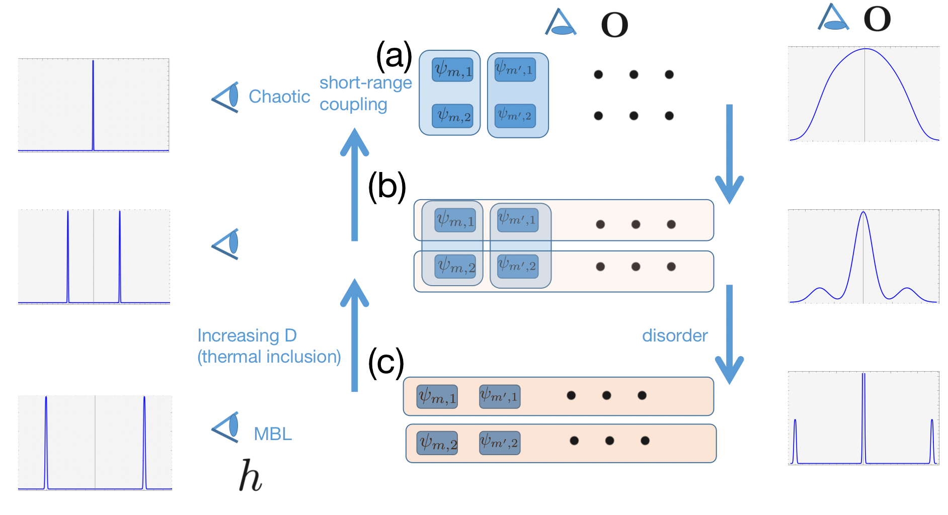
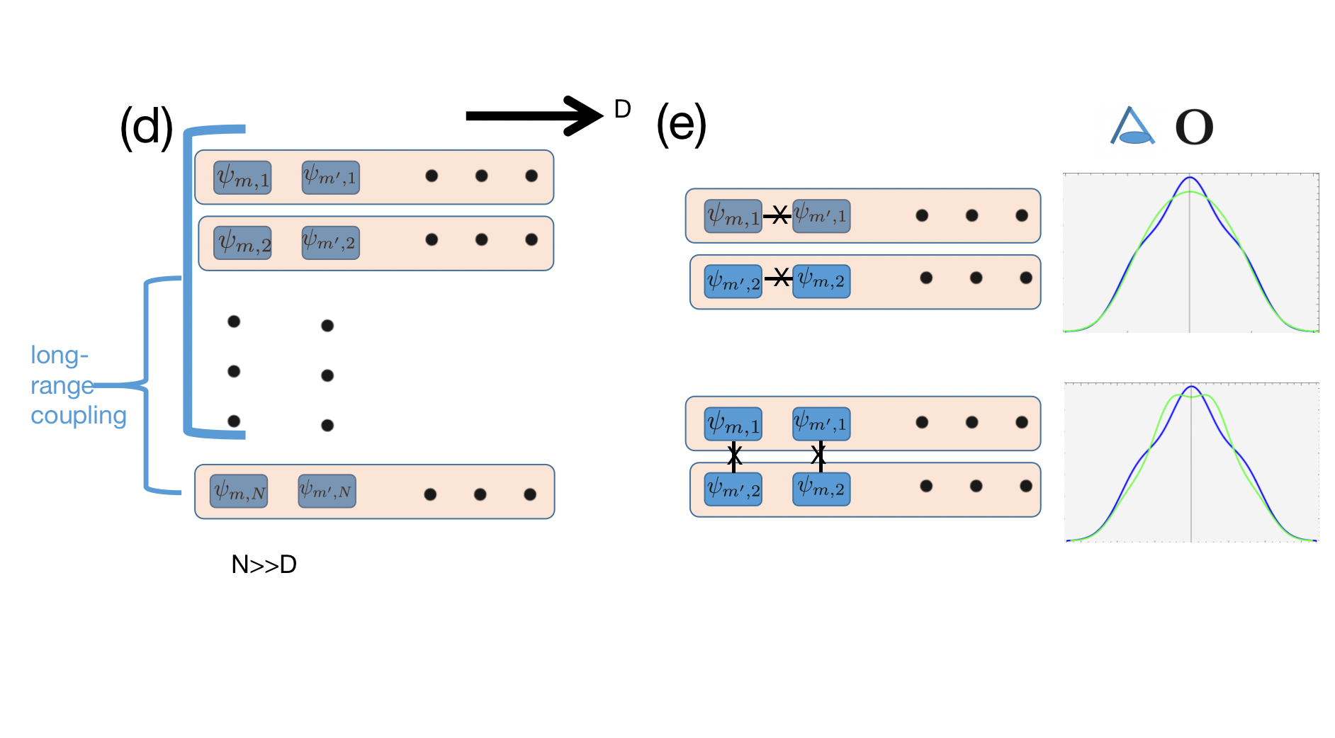
Figure 1: The eye-notations in left-side represent the estimation for the expectation of Hamiltonian (observable) $h=\psi_{m,1}\psi_{m^{\prime},1}^{*}\psi_{m,2}\psi_{m^{\prime},2}^{*}$, which mix the two symmetry sectors that are classified by two eigenvalues $\lambda_{1}$ and $\lambda_{2}$. (e) A more interlaced pattern as a result of the selected parameter set: For upper and lower panels we restrict $\overline{\psi_{m,1}\psi_{m^{\prime},1}^{*}}=\overline{\psi_{m,2}\psi_{m^{\prime},2}^{*}}=0$ and $\overline{\psi_{m,1}\psi_{m^{\prime},2}^{*}}=\overline{\psi_{m,2}\psi_{m^{\prime},1}^{*}}=0$ as indicated by the black lines with cross. In both these two cases, the transverse correlation plays the main role, i.e., the asymptotical degeneration between nonintegrable eigenstates. Also, these two cases share the almost same spectral (the only difference is that there is a small sink in the spectral of imaginary part of eigenvalues for the latter case). While the spetrals for the real part of eigenvalues all reflect the thermalization ($\mathcal{N}\sim(0,10.0396^{2})$ and $\mathcal{N}\sim(1.77636\times 10^{-15},16.9198^{2})$ for the two cases, repectively).

However, such many-body localization (as depicted in Fig.1(c)-(d)) never happen in our simulations, as can be seem from the nonzero eigenvalues (both the real and imaginary parts) in Figs.(3-5). Also, we see that, with the increase of $D$, in which case the effect of thermal inclusion becomes overwhelming that the disorders, the system quitely closes to the quantum chaos.

Figure 2: (a) The random Gaussian symmetry matrix up to $D=100$, $\frac{\sqrt{\lambda_{1}^{2}+\lambda_{2}^{2}}}{D}\frac{1}{\sqrt{2}}({\bf A}+{\bf A}^{T})$, with ${\bf A}$ be the $D\times D$ matrix whose entries are sampled from a standard normal distribution. The distribution of matrix elements follows $\mathcal{N}(-0.0112,0.031)$. The eigenvalue distribution is shown in (b). (c) The histogram plot satisfies the Wigner semicircle law. (d)-(e) show the level spacing statistic for GOE (the blue, red, orange, and Green lines correspond to GOE, GUE, GSE, and Poission, respectively). (f) shows the diagram corresponding to $D=500$.

Figure 3: (a)-(b) Real part and imaginary part of the approximated GOE matrix where the parameters of product variables are determined in terms of the second and fourth moments of GOE. (c)-(d) ((e)-(f)) show the real (imaginary) part of eigenvalues and its distribution. For lower $D$, we use the smoothed histogram diagram to reflect the probability density distribution. The distributions of real part and imaginary part of element follow $\mathcal{N}(5.55112\times 10^{-17},0.237598)$ and $\mathcal{N}(-1.38778\times 10^{-17},0.0813476)$, respectively. While the standard GOE follows $\mathcal{N}(0,0.15625)$.

Figure 4: The same with Fig.3 but for $D=6$. The distributions of real part and imaginary part of element follow $\mathcal{N}(0,0.904249)$ and $\mathcal{N}(1.23358\times 10^{-16},0.839433)$, respectively. While the standard GOE follows $\mathcal{N}(0,0.0648148)$.

Figure 5: The same with Fig.3 but for $D=8$. The distributions of real part and imaginary part of element follow $\mathcal{N}(1.11022\times 10^{-16},4.09099)$ and $\mathcal{N}(5.55112\times 10^{-17},4.05583)$, respectively. While the standard GOE follows $\mathcal{N}(0,0.0351563)$.

2.2 Singular nonrandom symmetry matrix

The second way is through a singular nonrandom symmetry matrix with real elements, which is generated in the following way: For Hilbert space dimension up to $D$, we construct the following singular nonrandom symmetry as an auxiliary matrix

$${\bf Q}=\frac{1}{\sqrt{\frac{1}{6}(D^{2}-1)}}\begin{pmatrix}D-1&D-2&\cdots&0\\ D-2&D-3&\cdots&1\\ \cdots\\ 0&-1&\cdots&D-1\\ \end{pmatrix},$$ (22)

where since the variance of elements within above matrix is $\frac{1}{D^{2}}\sum_{j=0}^{D-1}[\sum_{i=1}^{D}(D-j-i)^{2}]=\frac{1}{6}(D^{2}-1)$, there is a factor $\frac{1}{\sqrt{\frac{1}{6}(D^{2}-1)}}$ to make sure the variance of elements of ${\bf Q}$ is one. Then the matrix ${\bf Q}$ shares the following characters of a GOE random matrix (in the large-$D$ limit): $\overline{Q_{mm}}=0$, $\overline{Q_{mm}^{2}}=2$, $\overline{Q_{mm^{\prime}}}=0$, $\overline{Q_{mm^{\prime}}^{2}}=\frac{D-2}{D-1}\approx 1$, i.e., although the elements are not independent and identically distributed, they share the distributions of Gaussian random variables: $Q_{mm}\sim\mathcal{N}(0,2),\ Q_{mm^{\prime}}\sim\mathcal{N}(0,1)$. The only (and most explicit) difference is the singular matrix ${\bf Q}$ (whose determinant is zero and the whole matrix is Noninvertible) is a rank-2 matrix that has only two nonzero eigenvalues with the same absolute value. It can be viewed as a result of the proximity to integrability for a generic nonintegrable GOE matrix. As we know that for GOE random matrix the distribution of off-diagonal matrix elements is also Gaussian distributed with zero mean, and as it approaches integrability, the peak around zero becomes sharper[16], which can be seem from the emergent zero elements in the antidiagonal direction of ${\bf Q}$, and in the mean time the distribution becomes the combination of Gaussians. Also, the zero elements in antidiagonal direction in ${\bf Q}$ indicate the large number of linear-dependent eigenstates.

However, the (approximate) GOE matrix generated in the following way base on the diagonal elements of ${\bf Q}$ will not be singular anymore. This is because the probability for the generated matrix ${\bf H}$ be singular according to Lebesgue measure over $\mathbb{R}^{D^{2}}$ is zero, and the result is the same even for a probability measure (over the normally distributed $\mathbb{R}^{D^{2}}$) which is absolutely continuous with respect to Lebesgue measure. The non-singularity can be seem from the nondegenerated spectral as simulated below.

2.2.1 $D=4$

For a numerical simulation, we still choose $D=4$, then we have

$${\bf Q}=\left(\begin{array}[]{cccc}3\sqrt{\frac{2}{5}}&2\sqrt{\frac{2}{5}}&\sqrt{\frac{2}{5}}&0\\ 2\sqrt{\frac{2}{5}}&\sqrt{\frac{2}{5}}&0&-\sqrt{\frac{2}{5}}\\ \sqrt{\frac{2}{5}}&0&-\sqrt{\frac{2}{5}}&-2\sqrt{\frac{2}{5}}\\ 0&-\sqrt{\frac{2}{5}}&-2\sqrt{\frac{2}{5}}&-3\sqrt{\frac{2}{5}}\\ \end{array}\right)$$ (23)

whose nonzero eigenvalues are $\pm 2\sqrt{5}$, and $\overline{Q_{mm}^{2}}=2,\overline{Q_{mm^{\prime}}^{2}}=\frac{2}{3}$.

Then we only need to matching the classical analogy of diagonal elements of GOE matrix to the diagonal elements of ${\bf Q}$,

$$\lambda_{1}|\psi_{\alpha,1}|^{2}+\lambda_{2}|\psi_{\alpha,2}|^{2}=\frac{\lambda_{1}+\lambda_{2}}{D}+\sqrt{\lambda_{1}^{2}+\lambda_{2}^{2}}\frac{1}{D}Q_{11},$$ (24)

$$\lambda_{1}|\psi_{\beta,1}|^{2}+\lambda_{2}|\psi_{\beta,2}|^{2}=\frac{\lambda_{1}+\lambda_{2}}{D}+\sqrt{\lambda_{1}^{2}+\lambda_{2}^{2}}\frac{1}{D}Q_{44},$$

$$\lambda_{1}|\psi_{\eta,1}|^{2}+\lambda_{2}|\psi_{\eta,2}|^{2}=\frac{\lambda_{1}+\lambda_{2}}{D}+\sqrt{\lambda_{1}^{2}+\lambda_{2}^{2}}\frac{1}{D}Q_{22},$$

$$\lambda_{1}|\psi_{\gamma,1}|^{2}+\lambda_{2}|\psi_{\gamma,2}|^{2}=\frac{\lambda_{1}+\lambda_{2}}{D}+\sqrt{\lambda_{1}^{2}+\lambda_{2}^{2}}\frac{1}{D}Q_{33}.$$

In this case, we only need to solve $D/2$ parameters for the variables in Eq.(LABEL:goe) by setting $Y_{i}=X_{i}\ (i=1,\cdots,D)$. Then by choosing $(\lambda_{1},\lambda_{2})=(1,-1)$ and $\theta=\pi/4$, one of the possible set of real solution is $X_{1}=2.5232,X_{2}=-1.669$ (choosing different set of solution would leads to different statistic behaviors for small dimension $D$ but there will be minor difference for large $D$). Then we obtain the following (approximate) GOE matrix,

$${\bf H}=\left(\begin{array}[]{cccc}0.67082&-0.880801&0.524149&-0.440401\\ -0.880801&-0.67082&-0.333748&0.25\\ 0.524149&-0.333748&0.223607&-0.667497\\ -0.440401&0.25&-0.667497&-0.223607\\ \end{array}\right)$$ (25)

whose second moment of diagonal elements is $\overline{H_{mm}^{2}}=\frac{2}{D^{2}}(\lambda_{1}^{2}+\lambda_{2}^{2})=\frac{1}{4}$, but there is a deviation for second moment of off-diagonal elements $\overline{H_{mm^{\prime}}^{2}}=0.244$ from the GOE-predicted result $\frac{2}{D^{2}}=0.125$. We note that this deviation for the second moment of off-diagonal elements will be vanishingly small in large-$D$ limit.

Then the corresponding second moment of off-diagonal elements read

$$\overline{|\psi_{m,1}|^{2}|\psi_{m^{\prime},1}|^{2}}=0.0615259,$$ (26)

$$\overline{|\psi_{m,2}|^{2}|\psi_{m^{\prime},2}|^{2}}=0.0246067,$$

$$\overline{\psi_{m,1}\psi_{m^{\prime},1}^{*}}=-0.0238913,\ \overline{\psi_{m,2}\psi_{m^{\prime},2}^{*}}=0.0238913,$$

$$\overline{\psi_{m,1}\psi_{m^{\prime},2}^{*}}=\overline{\psi_{m,2}\psi_{m^{\prime},1}^{*}}=-0.0594421,$$

$$\overline{\psi_{m,1}\psi_{m^{\prime},1}^{*}\psi_{m,2}\psi_{m^{\prime},2}^{*}}=-0.0246067,$$

$$\overline{\psi_{m,1}\psi_{m^{\prime},2}^{*}\psi_{m,2}\psi_{m^{\prime},1}^{*}}=-0.0113555,$$

$$\overline{H_{mm^{\prime}}^{2}}=\overline{\sum_{i}\lambda_{i}\psi_{m,i}\psi^{*}_{m^{\prime},i}}=0.133063(\frac{\sum_{i}\lambda_{i}^{2}}{D^{2}}=0.125),$$

and the corresponding joint distribution in Eq.(LABEL:goe) is exactly satisfied,

$$\prod_{m}^{D}\frac{1}{\sqrt{4\pi}}e^{-\frac{1}{4}H_{mm}^{2}}\prod_{1\leq m<m^{\prime}\leq D}\frac{1}{\sqrt{2\pi}}e^{-\frac{1}{2}H_{mm^{\prime}}^{2}}=(2\pi)^{-\frac{D(D+1)}{4}}\frac{1}{(\sqrt{2})^{D}}e^{-\frac{1}{4}{\rm Tr}[{\bf H}{\bf H}^{T}]}=7.82922*10^{-6},$$ (27)

$$\prod_{i}^{D}e^{\frac{-\lambda^{2}_{i}}{2}}=\prod_{m}^{D}e^{-\frac{1}{2}H_{mm}^{2}}\prod_{1\leq m<m^{\prime}\leq D}e^{-H_{mm^{\prime}}^{2}}=e^{-{\rm Tr}{\bf H}{\bf H}^{T}/2}=0.0940494,$$

2.2.2 $D=8$

For $D=8$, the auxiliary matrix reads

$${\bf Q}=\left(\begin{array}[]{cccccccc}\sqrt{\frac{14}{3}}&2\sqrt{\frac{6}{7}}&5\sqrt{\frac{2}{21}}&4\sqrt{\frac{2}{21}}&\sqrt{\frac{6}{7}}&2\sqrt{\frac{2}{21}}&\sqrt{\frac{2}{21}}&0\\ 2\sqrt{\frac{6}{7}}&5\sqrt{\frac{2}{21}}&4\sqrt{\frac{2}{21}}&\sqrt{\frac{6}{7}}&2\sqrt{\frac{2}{21}}&\sqrt{\frac{2}{21}}&0&-\sqrt{\frac{2}{21}}\\ 5\sqrt{\frac{2}{21}}&4\sqrt{\frac{2}{21}}&\sqrt{\frac{6}{7}}&2\sqrt{\frac{2}{21}}&\sqrt{\frac{2}{21}}&0&-\sqrt{\frac{2}{21}}&-2\sqrt{\frac{2}{21}}\\ 4\sqrt{\frac{2}{21}}&\sqrt{\frac{6}{7}}&2\sqrt{\frac{2}{21}}&\sqrt{\frac{2}{21}}&0&-\sqrt{\frac{2}{21}}&-2\sqrt{\frac{2}{21}}&-\sqrt{\frac{6}{7}}\\ \sqrt{\frac{6}{7}}&2\sqrt{\frac{2}{21}}&\sqrt{\frac{2}{21}}&0&-\sqrt{\frac{2}{21}}&-2\sqrt{\frac{2}{21}}&-\sqrt{\frac{6}{7}}&-4\sqrt{\frac{2}{21}}\\ 2\sqrt{\frac{2}{21}}&\sqrt{\frac{2}{21}}&0&-\sqrt{\frac{2}{21}}&-2\sqrt{\frac{2}{21}}&-\sqrt{\frac{6}{7}}&-4\sqrt{\frac{2}{21}}&-5\sqrt{\frac{2}{21}}\\ \sqrt{\frac{2}{21}}&0&-\sqrt{\frac{2}{21}}&-2\sqrt{\frac{2}{21}}&-\sqrt{\frac{6}{7}}&-4\sqrt{\frac{2}{21}}&-5\sqrt{\frac{2}{21}}&-2\sqrt{\frac{6}{7}}\\ 0&-\sqrt{\frac{2}{21}}&-2\sqrt{\frac{2}{21}}&-\sqrt{\frac{6}{7}}&-4\sqrt{\frac{2}{21}}&-5\sqrt{\frac{2}{21}}&-2\sqrt{\frac{6}{7}}&-\sqrt{\frac{14}{3}}\\ \end{array}\right).$$ (28)

Then similar procedure leads to the commensurate product basis as shown in Eq.(LABEL:goe) with parameters $X_{1}=3.63596,X_{2}=3.11909,X_{3}=2.49744,X_{4}=1.65703$, and the corresponding (approximate) GOE matrix reads

$${\bf H}=\left(\begin{array}[]{cccccccc}0.381881&-0.414747&0.211095&-0.269874&0.191669&-0.269874&0.165406&-0.269874\\ -0.414747&-0.381881&-0.253722&0.0625&-0.234295&0.0625&-0.208032&0.0625\\ 0.211095&-0.253722&0.272772&-0.382443&0.175517&-0.253722&0.149254&-0.253722\\ -0.269874&0.0625&-0.382443&-0.272772&-0.234295&0.0625&-0.208032&0.0625\\ 0.191669&-0.234295&0.175517&-0.234295&0.163663&-0.34359&0.129827&-0.234295\\ -0.269874&0.0625&-0.253722&0.0625&-0.34359&-0.163663&-0.208032&0.0625\\ 0.165406&-0.208032&0.149254&-0.208032&0.129827&-0.208032&0.0545545&-0.291064\\ -0.269874&0.0625&-0.253722&0.0625&-0.234295&0.0625&-0.291064&-0.0545545\\ \end{array}\right)$$ (29)

whose second moment of diagonal elements is $\overline{H_{mm}^{2}}=\frac{2}{D^{2}}(\lambda_{1}^{2}+\lambda_{2}^{2})=\frac{4}{64}=0.0625$, and the second moment of off-diagonal elements is $\overline{H_{mm^{\prime}}^{2}}-\overline{H_{mm^{\prime}}}^{2}=0.029952$, which becomes closer to the GOE-predicted result $\frac{2}{D^{2}}=0.03125$.

Then the corresponding second moment of off-diagonal elements read

$$\overline{|\psi_{m,1}|^{2}|\psi_{m^{\prime},1}|^{2}}=0.0162997,$$ (30)

$$\overline{|\psi_{m,2}|^{2}|\psi_{m^{\prime},2}|^{2}}=0.0057852,$$

$$\overline{\psi_{m,1}\psi_{m^{\prime},1}^{*}}=-0.013754,\ \overline{\psi_{m,2}\psi_{m^{\prime},2}^{*}}=0.0673254,$$

$$\overline{\psi_{m,1}\psi_{m^{\prime},2}^{*}}=\overline{\psi_{m,2}\psi_{m^{\prime},1}^{*}}=-0.0123096,$$

$$\overline{\psi_{m,1}\psi_{m^{\prime},1}^{*}\psi_{m,2}\psi_{m^{\prime},2}^{*}}=-0.00243698,$$

$$\overline{\psi_{m,1}\psi_{m^{\prime},2}^{*}\psi_{m,2}\psi_{m^{\prime},1}^{*}}=-0.00163519,$$

$$\overline{H_{mm^{\prime}}^{2}}=\overline{\sum_{i}\lambda_{i}\psi_{m,i}\psi^{*}_{m^{\prime},i}}=0.020385(\frac{\sum_{i}\lambda_{i}^{2}}{D^{2}}=0.03125),$$

and the corresponding joint distribution in Eq.(LABEL:goe) is exactly satisfied,

$$\prod_{m}^{D}\frac{1}{\sqrt{4\pi}}e^{-\frac{1}{4}H_{mm}^{2}}\prod_{1\leq m<m^{\prime}\leq D}\frac{1}{\sqrt{2\pi}}e^{-\frac{1}{2}H_{mm^{\prime}}^{2}}=(2\pi)^{-\frac{D(D+1)}{4}}\frac{1}{(\sqrt{2})^{D}}e^{-\frac{1}{4}{\rm Tr}[{\bf H}{\bf H}^{T}]}=1.37728\times 10^{-16},$$ (31)

$$\prod_{i}^{D}e^{\frac{-\lambda^{2}_{i}}{2}}=\prod_{m}^{D}e^{-\frac{1}{2}H_{mm}^{2}}\prod_{1\leq m<m^{\prime}\leq D}e^{-H_{mm^{\prime}}^{2}}=e^{-{\rm Tr}{\bf H}{\bf H}^{T}/2}=0.263487.$$

Figure 6: (a)-(c) show the results for $D=4$, where the entries distribution follows $\mathcal{N}(-0.0709444,0.162383^{2})$. (d)-(f) show the results for $D=8$, where the distribution of elements of ${\bf H}$ follows $\mathcal{N}(-0.0709444,0.162383^{2})$. (g)-(i) show the results for $D=14$, where the distribution of elements of ${\bf H}$ follows $\mathcal{N}(-0.0530054,0.0846555^{2})$. Comparing to the method that identifying the parameters by considering the second the fourth moments of Gaussian variables $\psi_{m,i}$, as shown in Fig.3, the method that matching the diagonal elements of the corresponding singular matrix is more efficient as it only require to solve $D/2$ parameters. The eigenvalue distribution is also different from that in Fig.3 and Fig.2, where the probability density distribution (the spectral) for the eigenvalues becomes asymmetry, and a three-peak pattern appears in the spectral with the increase of $D$. For a comparasion, we note that for standard GOE the distributions follow $\mathcal{N}(0,0.15625)$, $\mathcal{N}(0,0.0351563)$, and $\mathcal{N}(0,0.022)$, for $D=4,8,10$, respectively. (j)The ratios $\mathcal{R}_{1}$ and $\mathcal{R}_{2}$ for these three sizes.

Figure 7: The same with Fig.6 where (a)-(c), (d)-(f), (g)-(h) correspond to $D=20,30,34$, respectively. With the increase of $D$, $\mathcal{R}_{2}$ exponentially increase while $\mathcal{R}_{1}$ approaches to one with logarithmically slow speed, e.g., for $D=20$, $\mathcal{R}_{2}=1239.18,\mathcal{R}_{1}=1.43874$.

2.2.3 $D=14$

For $D=14$, Then the corresponding second moment of off-diagonal elements read

$$\overline{|\psi_{m,1}|^{2}|\psi_{m^{\prime},1}|^{2}}=-0.00499347,$$ (32)

$$\overline{|\psi_{m,2}|^{2}|\psi_{m^{\prime},2}|^{2}}=0.0520892,$$

$$\overline{\psi_{m,1}\psi_{m^{\prime},1}^{*}}=0.0054854,\ \overline{\psi_{m,2}\psi_{m^{\prime},2}^{*}}=0.00283132,$$

$$\overline{\psi_{m,1}\psi_{m^{\prime},2}^{*}}=\overline{\psi_{m,2}\psi_{m^{\prime},1}^{*}}=-0.00300621,$$

$$\overline{\psi_{m,1}\psi_{m^{\prime},1}^{*}\psi_{m,2}\psi_{m^{\prime},2}^{*}}=-0.0006154,$$

$$\overline{\psi_{m,1}\psi_{m^{\prime},2}^{*}\psi_{m,2}\psi_{m^{\prime},1}^{*}}=-0.000330711,$$

$$\overline{H_{mm^{\prime}}^{2}}=\overline{(\sum_{i}\lambda_{i}\psi_{m,i}\psi^{*}_{m^{\prime},i})^{2}}=0.00591522(\frac{\sum_{i}\lambda_{i}^{2}}{D^{2}}=0.0102041),$$

By estimating the ratios $\mathcal{R}_{1}=\frac{\overline{\psi_{m,1}\psi_{m^{\prime},1}^{*}\psi_{m,2}\psi_{m^{\prime},2}^{*}}}{\overline{\psi_{m,1}\psi_{m^{\prime},1}^{*}}\ \overline{\psi_{m,2}\psi_{m^{\prime},2}^{*}}}$ and $\mathcal{R}_{2}=\frac{\overline{\psi_{m,1}\psi_{m^{\prime},2}^{*}\psi_{m,2}\psi_{m^{\prime},1}^{*}}}{\overline{\psi_{m,1}\psi_{m^{\prime},2}^{*}}\ \overline{\psi_{m,2}\psi_{m^{\prime},1}^{*}}}$ in Eqs.(LABEL:72901,LABEL:72902,LABEL:72903), as shown in Fig.6(j) we can obtain the conclusion in opposite with the above method: with the increase of $D$, the transverse correlation becomes overwhelming. Although it seems there is a proximity to integrability with the increase of $D$ as the average for off-diagonal elements $\overline{H_{mm^{\prime}}^{2}}$ deviates away from the GOE prediction $\frac{\sum_{i}\lambda_{i}^{2}}{D^{2}}$ and thus the off-diagonal elements deviate away from Gaussian, the off-diagonal elements indeed form another Gaussian, whose average for off-diagonal elements $\overline{H_{mm^{\prime}}^{2}}$ approaches $\frac{\sum_{i}\lambda_{i}^{2}}{2D^{2}}$ in the large $D$ limit.

As shown in Fig.7, for larger $D$, $\overline{\psi_{m,1}\psi_{m^{\prime},1}^{*}\psi_{m,2}\psi_{m^{\prime},2}^{*}}$ reduces to zero, while the second moment of off-diagonal elements will change from almost equal to that of standard GOE to half of that of standard GOE: $\overline{\sum_{i}\lambda_{i}\psi_{m,i}\psi^{*}_{m^{\prime},i}}=\frac{\sum_{i}\lambda_{i}^{2}}{D^{2}}\rightarrow\overline{\sum_{i}\lambda_{i}\psi_{m,i}\psi^{*}_{m^{\prime},i}}=\frac{\sum_{i}\lambda_{i}^{2}}{2D^{2}}$. That means, although there is a proximity to integrability for the off-diagonal elements as can be seem from the spectral which deviates from the Gaussian shape and there is a broadened peak in the middle, the maximal number of linear independent eigenvectors is still $D$.

2.3 conclusion for the two methods

Now we have introduced two methods to constructing the approximate GOE matrix which shares the same main characters, in terms of the global statistic behaviors, of a standard GOE matrix. For first method by matching the second and fourth moments, although the mutually independence between eigenket-labelled vectors (for an unique eigenvalue) is enhanced with the increase of $D$ (i.e., $\mathcal{R}_{2}\rightarrow 0$ in $D\rightarrow\infty$ limit), the average $\overline{\psi_{m,1}\psi_{m^{\prime},1}^{*}\psi_{m,2}\psi_{m^{\prime},2}^{*}}$ increase with the increasing $D$, and that is due to the rised correlations in longitudinal direction (as shown diagrammatically in Fig.1) between two eigenvalues which reveals the effect of thermal inclusion. Thus in this case, the enlarged size $D$ has an effect opposite to the enhanced disorder (which will suppress the effect of thermal inclusion and promote to integrable side[17]).

While for lower $D$ with the extensive symmetry in the longitudinal direction, the enhanced $\mathcal{R}_{2}$ is due to the imbalance effect between $\langle\lambda_{1}|m\rangle$ and $\langle\lambda_{1}|m^{\prime}\rangle$ (or $\langle\lambda_{2}|m\rangle$ and $\langle\lambda_{2}|m^{\prime}\rangle$), and the induced MBL can be understood as a result of the translational symmetry breaking along the transverse direction induced by the well-performed multiplied (superposed) quantum state representation in terms of the good quantum number for noninteracting (interacting) integrable system. This is depicted in (c) of Fig.1, where the extended symmetry is guaranteed by the large $N(\gg D)$, and thus is always a lowest energy state even there is ergodicity that can be reached at a large $N(\gg D)$ as long as the integrable eigenstates are approximately mutually orthogonal in $N\rightarrow\infty$ limit.

Also, since for the model we discuss, the ergodic-breaking (or the asymptotical degenerate in transverse direction) is not due to the long-range type coupling along the transverse direction (although this is also possible but of another mechanism), but a more complex four-point correlation configuration between $\psi_{m,1}\psi_{m^{\prime},2}^{*}$ and $\psi_{m,2}\psi_{m^{\prime},1}^{*}$ (which does not appear in the orignal Hamiltonian describing the system), and we note that this correlation configuration can perfectly coexist with the orthogonal condition between two integrable eigenstates ($\overline{\psi_{m,1}\psi^{*}_{m,2}}=0,\forall m$). Thus, specially, the correlation between $\psi_{m,1}\psi_{m^{\prime},2}^{*}$ and $\psi_{m,2}\psi_{m^{\prime},1}^{*}$ has a competition effect with that between $\psi_{m,1}\psi_{m^{\prime},1}^{*}$ and $\psi_{m,2}\psi_{m^{\prime},2}^{*}$, where the latter one can be diluted by the extensive symmetry along the longitudinal direction. In real materials, this can be related to the ideal (or even quantitatively) electronic transport in the long-time (low-frequency limit), e.g., the Drude weight as an evidence of finite conductivity at zero frequency can be the result of robust temporal fluctuation (revealed by the off-diagonal elements) as a response to the external disorders[15].

However, different to the simply diagnozed ergodicity-breaking due to the persistent long-time fluctuation as a response to external disorder, the proximity to the integrability in our model (although never reaches the MBL) is due to the more complex correlation configuration that involving different symmetry sectors (with respect to the observable ${\bf O}$), and the system always be thermalized in the long-time limit as evidenced by the nondegenerated eigenvalue spectral (Fig.7) where the asymptotic degeneracy to the zero-energy level more and more slow with increasing $D$ and the center peak in spectral never reduced to a Dirac-Delta one (where a thermal inclusion plays a key effect). Thus this is more similar to the case of suppressed quantum quantum chaos can be suppressed by strong coupling between different subsystems[8].

While in the integrable (MBL) case, there will be three-peak spectral as shown in the right-side of Fig.1, where the MBL here can be regarded as a breaking of ergodicity due to the effect of couplings (or disorders) within each integrable eigenstates (indicated by horizontal orange bars), and when here is infinite ($N\gg D$) integrable eigenstates each bar will behaves classically and tends to a symmetry sector. This is also in the same principle with ergodicity-breaking induced by asymptotically ($N\rightarrow\infty$) generated self-sustained oscillations among classical nonlinear systems through the a small coupling[9].

3 IPR, NPR, and the reference basis of the Hilbert space

Figure 8: (a,b) Spectrum for the $|\psi_{i\ell,1(2)}|^{2}$ and $|\psi_{i\ell,1(2)}|^{4}$, respectively. (c,d)Inverse participation ratio (IPR) and normalized participation ratio (NPR) for all eigenstates sampled from $\psi_{i\ell,1(2)}$, respectively, for integrable case. (e,f)The same with (c,d) but for nonintegrable case.

The expressions for inverse participation ratio (IPR) and normalized participation ratio (NPR) read

$${\rm NPR}=\frac{1}{L\sum^{L}_{i}|\psi_{i\ell,1(2)}|^{4}},$$ (33)

$${\rm IPR}=\frac{\sum^{L}_{i}|\psi_{i\ell,1(2)}|^{4}}{(\sum^{L}_{i}|\psi_{i\ell,1(2)}|^{2})^{2}},$$

where for each eigenstate the subscript $i$ denote the set of discrete local coordinators which is selected (randomly or elaborately) from the eigenstates of an eigenvalue. Note that the IPR and NPR are reference basis-dependent quantities, and the discrete set of coordinators labeled by $i$ is the reference basis of the Hilbert space[8]. Fig.8(a)-(b) show the random selection results for the squared and quadruplicated eigenstates for system size $L=500(\geq d)$. In integrable case with randomly selected local coordinators, $\sum^{L}_{i}|\psi_{i\ell,1(2)}|^{4}\sim L$, and $\sum^{L}_{i}|\psi_{i\ell,1(2)}|^{2}\sim L$, i.e., the difference between squared and quadruplicated eigenstates can be neglected for large system size. This is shown in Fig.8(c)-(d), where ${\rm NPR}\propto L^{-2}$, and ${\rm IPR}\propto L^{-1}$.

When the local coordinates are selected under some restriction, and results in a local conservation for the quadruplicated eigenstates $\sum^{L}_{i}|\psi_{i\ell,1(2)}|^{4}=1$, while the squared eigenstates still satisfies $\sum^{L}_{i}|\psi_{i\ell,1(2)}|^{2}\sim L$. There could at most be $(L-1)$ terms $|\psi_{i\ell,1(2)}|^{4}$ be the local conserved quantities where each one corresponds to an excited state. As a result of elaborated set of coordinates, there is are correlations between $|\psi_{i\ell,1(2)}|^{2}$ terms within $|\psi_{i\ell,1(2)}|^{4}$, i.e.,

$$\overline{|\psi_{i\ell,1(2)}|^{4}}=\overline{|\psi_{i\ell,1(2)}|^{2}|\psi_{i\ell,1(2)}|^{2}}=L^{-1}\neq\overline{|\psi_{i\ell,1(2)}|^{2}}\ \overline{|\psi_{i\ell,1(2)}|^{2}}\ (\overline{|\psi_{i\ell,1(2)}|^{2}}=1),$$ (34)

While for the summation $\sum^{L}_{i}|\psi_{i\ell,1(2)}|^{2}\sim L$ as an extensive quantity, owns degenerated ground states. This is shown in Fig.8(e)-(f), where ${\rm NPR}\propto L^{-1}$, and ${\rm IPR}\propto L^{-2}$.

So there is an elaborated normalization over the squared eigenstates and realizing an uniform superposition in terms of the fourth moment, by enforcing a correlation between the squared eigenstates. Thus the competitions between the integrability and chaos here can be described by an embedding model $\hat{h}=\sum^{L}_{i}|\psi_{i\ell,1(2)}|^{4}+\sum^{L}_{i}|\psi_{i\ell,1(2)}|^{2}$, where in first term $|\psi_{i\ell,1(2)}|^{4}=|\psi_{i\ell,1(2)}|^{2}\hat{P}_{i}$ with $|\psi_{i\ell,1(2)}|^{2}$ the local term and $\hat{P}_{i}=|\psi_{i}\rangle\langle\psi_{i}|$ the local projection operator (microcanonical ensemble density matrix).

The thermalized pure states also results in

$$\langle\phi|\sum_{i}|\psi_{i\ell,1(2)}|^{2}|\phi\rangle={\rm Tr}[(\sum_{i}\hat{P}_{i})(\sum_{i}|\psi_{i\ell,1(2)}|^{2})],$$ (35)

in which case the local projection on each local site $\hat{P}_{i}$ is a local conserved quantity, and the full or partial trace of microcanonical density matrix follows the Gibbs representation,

$${\rm Tr}|\phi\rangle\langle\phi|={\rm Tr}[\sum_{i}\hat{P}_{i}],$$ (36)

and the average over microcanonical ensemble $MC_{j}$ is

$$\overline{\langle\phi|\sum_{i}\hat{P}_{i}|\phi\rangle}=\sum_{k,l}\overline{c_{k}^{*}c_{l}}\langle\phi_{k}|\sum_{i}\hat{P}_{i}|\phi_{l}\rangle=\langle\sum_{i\in MC_{j}}\hat{P}_{i}\rangle_{MC_{j}},$$ (37)

where $\overline{c_{k}^{*}c_{l}}=\frac{\delta_{kl}}{d_{MC_{j}}}$ with $d_{MC_{j}}=\frac{1}{\sum_{i\in MC_{j}}|\psi_{i\ell,1(2)}|^{2}}$ the dimension of the subspace spanned by the microcanonical density corresponding to one of the orthogonal eigenstates. In the limit of $\overline{c_{k}^{*}c_{l}}\approx c_{k}^{*}c_{l}$, i.e., the $d_{MC_{j}}\approx\frac{1}{\overline{|\psi_{i\ell,1(2)}|^{2}}}$ approaches the minimal value, which corresponds to narrow microcanonical shell and small fluctuation of energy density.

The expression of local projection operator is similar to weak perturbation, and the summation over local sites leads to a term similar to the Majumdar-Ghosh model[12], $\sum_{i}\hat{P}_{i}$, with maximal number of orthogonal eigenstates be $\sim{\rm ploy}[L]$, and minimal number of orthogonal eigenstates be two (where all the other $({\rm ploy}[L]-2)$ eigenstates are the degenerated ground states corresponds to zero eigenvalue). For the case $\sum_{i}\hat{P}_{i}$, has a maximal number of orthogonal eigenstates or order $O({\rm ploy}[L])$, the microcanonical ensemble density matrix is equivalent to the Gibbs representation in thermodynamic limit.

In terms of the large effective dimension of a pure state, $\frac{D_{eff}}{d_{MC_{j}}}\sim{\rm ploy}[\frac{1}{L}]$ in nonintegrable case and $\frac{D_{eff}}{d_{MC_{j}}}\sim e^{-L}$ in integrable case. The completely thermalized pure states correspond to the case that the subspace dimension $d_{MC_{j}}$ spanned by the pure states of the microcanonical energy shell labeled by $j$ reaches its minimal value, while the variance $\overline{c_{k}^{*}c_{l}}$ reaches its maximal value. In this case, there is not degenerated ground states in the subspace of $\sum_{i}\hat{P}_{i}$, and the eigenstates of Hilbert space and that of the subspace spanned by nonthermal states (if exist) have finite and zero expectation values on each individual local term $\hat{P}_{i}$, respectively.

In another scheme where the normalization is performed for the squared eigenstates, in which case the thermodynamic limit $L\rightarrow\infty$ corresponds to maximal dimension $d_{MC_{j}}$ and maximal variance of energy density[6]. In this case, there are few microcanonical ensembles and each one of them corresponds to an extensive quantity $\sum_{i\in MC_{j}}\hat{P}_{i}$. The correlations between abitarily two extensive quantities arised with the increasing $d_{MC_{j}}$[6], during which process

Then the polynomially small $\frac{D_{eff}}{d_{MC_{j}}}$ implies thermalization of the pure state basis (i.e., the eigenstate of the whole system or the initial state average over the $i$-dependent states). In the mean time, $D_{eff}=D[\overline{\sum^{d}_{\ell}|\psi_{i\ell,1(2)}|^{4}}]^{-1}$ also reflects the account of eigenstate covered by the pure state, which is $D_{eff}={\rm poly}[L]$. In this case, $|\psi_{i\ell,1(2)}|^{4}$ are $d$ extensive quantities labeled by $\ell$, which are mutually not commute and hence cannot be simultaneously measured[6].

Figure 9: The first column shows the variance of local observable $\hat{O}_{1}$ with different sample ranges. The second column shows ratio of variances of nearby system sizes $\frac{L_{n}}{L_{n+1}}$ with different sample ranges.

Figure 10: The same with Fig.9 but for the local observable $\hat{O}_{2}$.

3.1 Variance of local observable

Next we consider the weak ETH diagnosis in terms of variance of above-mentioned local observable.

We consider the thermalized system in normalized form as $\frac{1}{L}\sum_{i}^{L+1}|\psi_{i\ell,1(2)}|^{2}=\frac{1}{L}$, which provides the pure state basis that thermaized with respect to the local observable. In thermodynamic limit, there are $L$ mutually independent $|\psi_{i\ell,1(2)}|^{2}$ terms each corresponds to an individual eigenstates with nonzero eigenvalue, and there is an additional term $|\psi_{i=(L+1),\ell,1(2)}|^{2}=(1-\sum_{i}^{L}|\psi_{i\ell,1(2)}|^{2})$ corresponding to the nonthermal state, and all these eigenstates form the Hilbert space.

In the case where the weak ETH holds, the expectation of local observable reads (in thermodynamic limit)

$$\hat{O}_{1} =\overline{\langle\phi|\frac{1}{L}\sum_{i}^{L}|\psi_{i\ell,1(2)}|^{2}|\phi\rangle}$$ (38)

$$=\sum_{k,l}\overline{c^{*}_{k}c_{l}}\langle\phi_{k}|\frac{1}{L}\sum_{i}^{L}|\psi_{i\ell,1(2)}|^{2}|\phi_{l}\rangle$$

$$=\sum_{k,l}\frac{1}{d_{MC_{j}}}\langle\phi_{k}|\frac{1}{L}\sum_{i}^{L}|\psi_{i\ell,1(2)}|^{2}|\phi_{l}\rangle$$

$$={\rm Tr}[(\frac{1}{L}\sum_{i}^{L}|\psi_{i\ell,1(2)}|^{2})(\frac{1}{d_{MC_{j}}}\sum_{k\in MC_{j}}^{d_{MC_{j}}}\hat{P}_{k})],$$

where $d_{MC_{j}}\sim e^{L}$ is the dimension of microcanonical energy shell, and the summation of local projection terms plays the role of microcanonical density matrix here. In this case the expectation value of local observable equals the microcanonical ensemble average. We assume that the product with microcanonical density matrix projecting the system $(\frac{1}{L}\sum_{i}^{L+1}|\psi_{i\ell,1(2)}|^{2}-1)$ into a Gaussian system where the terms $|\psi_{i\ell,1(2)}|^{2}$ (for $i=1,\cdots,L$) together with $(|\psi_{i=(L+1),\ell,1(2)}|^{2}-1)$ are Gaussian distributed with zero mean and unit variance. Due to the large magnitude of $d_{MC_{j}}$ here compares to $L$, it allows the microcanonical density matrix further projecting each term label by $i$ into a Gaussian distributed variable, so that during the simulation we set a finite range for the random samples $|\psi_{i\ell,1(2)}|^{2}$.

For the case of weak ETH, we can treat each individual term at site $i$ as a long-time averaged result over the time window defined by a certain symmetry sector, and all these sectors are embeded one-by-one with the ascended order of sector size, which meke sure all these $L$ terms as a whole is of a single sector and thus satisfies the ETH. This can be expressed as

$$\hat{O}_{1} ={\rm Tr}[(\frac{1}{L}\sum_{i}^{L}|\psi_{i\ell,1(2)}|^{2})(\frac{1}{d_{MC_{j}}}\sum_{k\in MC_{j}}^{d_{MC_{j}}}\hat{P}_{k})]$$ (39)

$$=\int^{T}_{0}dt[(\frac{1}{L}\sum_{i}^{L}|\psi_{i\ell,1(2)}|^{2})(\frac{1}{d_{MC_{j}}}\sum_{k\in MC_{j}}^{d_{MC_{j}}}\hat{P}_{k}(t))]$$

$$=\frac{1}{L}\sum_{i}^{L}|\psi_{i\ell,1(2)}|_{t}^{2}(c_{i})_{t},$$

where the projection-induced coefficients $c_{i}$ form an orthogonal basis, and $c_{i}^{*}c_{j}=\frac{\delta_{ij}}{\sum_{t}\frac{1}{L^{2}}|\psi_{i\ell,1(2)}|^{4}}$.

As a result of Gaussian distribution, the average over corresponding time interval is $\overline{|\psi_{i\ell,1(2)}|_{t}^{4}(c_{i}^{*}c_{i})_{t}}=\frac{1}{d_{i}}$, and can be projected to a subspace with dimension $d_{i}$, where the summation of diagonal elements is 1. This make sure the norm $|c_{i}|$ is mutually independent for different sites. For arbitarily two sites $i$ and $j$, $\overline{|\psi_{i\ell,1(2)}|_{t}^{2}|\psi_{j\ell,1(2)}|_{t}^{2}(c_{1}^{*}c_{2})_{t}}=\overline{|\psi_{i\ell,1(2)}|_{t}^{2}(c^{*}_{1})_{t}}\ \overline{|\psi_{j\ell,1(2)}|_{t}^{2}(c_{2})_{t}}=0$, thus the mutually independence between different sites requires small fluctuation of the directions of $(c_{i})_{t}$ during the time evolution ($\frac{(c_{i})_{t}}{|c_{i}|_{t}}$ be independent of time). There is a set of integrable eigenstates in a nonintegrable system, and the weak fluctuation of coefficient directions impose $[|\psi_{i\ell,1(2)}|^{2},\frac{(c_{i})_{t}}{|c_{i}|_{t}}]\sim 0$. For a density operator $\hat{\rho}_{t}$ soly controlling the directions of the coefficients $c_{i}$, then the weak fluctuation of the density operator is connected to the weak variance of the energy density ${\rm Tr}[\hat{h}_{t}\hat{\rho}_{0}]$, which also implies the narrow microcanonical window, ${\rm Tr}[(\frac{1}{L}\sum_{i}^{L}|\psi_{i\ell,1(2)}|^{2})\hat{\rho}_{t}]=\langle(\frac{1}{L}\sum_{i}^{L}|\psi_{i\ell,1(2)}|^{2})\rangle_{MC_{j}}$. In this case the shell dimension $d_{MC_{j}}$ is reduced. That is to say, the reduced $d_{MC_{j}}$ lower the probability of the generation of coherence pattern as well as the delocalization in terms of the superpositions between eigenstates withi the shell. We will introduce below a protocol to realizing such suppression of coherence in the case of thermodynamic limit where the $d_{MC_{j}}$ and shell width is fixed, which is by endowing the sample range a linearly dependence with the system size.

As an example, for the local terms at sites $i$ and $j$,

$$\sum_{t}[\frac{1}{L^{2}}|\psi_{i\ell,1(2)}|_{t}^{4}(c_{1}^{*}c_{1})_{t}]=(\sum_{t}\frac{1}{L^{2}}|\psi_{i\ell,1(2)}|_{t}^{4})c_{1}^{*}c_{1}=1,$$ (40)

$$\sum_{t}[\frac{1}{L^{2}}|\psi_{j\ell,1(2)}|_{t}^{4}(c_{2}^{*}c_{2})_{t}]=(\sum_{t}\frac{1}{L^{2}}|\psi_{j\ell,1(2)}|_{t}^{4})c_{2}^{*}c_{2}=1,$$

$$\sum_{t}[\frac{1}{L^{2}}|\psi_{i\ell,1(2)}|_{t}^{2}|\psi_{j\ell,1(2)}|_{t}^{2}(c_{1}^{*}c_{2})_{t}]=\sum_{t}[\frac{1}{L^{2}}|\psi_{i\ell,1(2)}|_{t}^{2}|\psi_{j\ell,1(2)}|_{t}^{2}](c_{1}^{*}c_{2})=0,$$

where the projections to sites $i$ and $j$ results in the coefficients $c_{1}$ and $c_{2}$, respectively.

For the case that violating the weak ETH,

$$\hat{O}_{2} =\langle\phi|\frac{1}{L}\sum_{i}^{L+1}|\psi_{i\ell,1(2)}|^{2}|\phi\rangle$$ (41)

$$=\sum_{k,l}c^{*}_{k}c_{l}\langle\phi_{k}|\frac{1}{L}\sum_{i}^{L+1}|\psi_{i\ell,1(2)}|^{2}|\phi_{l}\rangle$$

$$={\rm Tr}[(\frac{1}{L}\sum_{i}^{L+1}|\psi_{i\ell,1(2)}|^{2})(\frac{1}{d_{MC_{j}}}\sum_{k\in MC_{j}}^{d_{MC_{j}}}\hat{P}_{k}(t))],$$

where $\hat{P}_{k}(t)=e^{iH_{t}t}\hat{P}_{k}e^{-iH_{t}t}$. Here the diffusive pure state basis generates the coherence in terms of the random phases and amplitudes.

We further consider the case that there is only one microcanonical ensemble, then the variance of the local observable as a summation of local terms provides a diagnosis of ETH[12]. We firstly consider the purely thermalized system, where the local observable consists of only the $L$ mutually independent locally conserved quantities. Then for completely thermalized (strong ETH) and incompletely thermalized case (weak ETH), the variances read

$${\rm Var}[\hat{O}]_{1}=\overline{\frac{1}{L^{2}}(\sum_{i}^{L}|\psi_{i\ell,1(2)}|^{2})^{2}}=\frac{1}{L^{2}}\sum_{i}^{L}|\psi_{i\ell,1(2)}|^{4},$$ (42)

$${\rm Var}[\hat{O}]_{2}=\frac{1}{L^{2}}\sum_{i}^{L}|\psi_{i\ell,1(2)}|^{4}+\frac{1}{L^{2}}|(1-\sum_{i}^{L}|\psi_{i\ell,1(2)}|^{2})|^{2},$$

In the mean time, we fix the range of random variables $|\psi_{i\ell,1(2)}|^{2}$ within $[-K,K]$, then our numerical simulation shows that the variance exhibits exponential decay with the increase of $L$, i.e., ${\rm Var}[\hat{O}](L)\sim{\rm Exp}[-L]$. Furthermore, we found that the variance of local observable without containing any nonlocal conserved quanty reads

$${\rm Var}[\hat{O}]_{1}[L=n]=\frac{n+1}{n}{\rm Var}[\hat{O}]_{1}[L=n+1].$$ (43)

This is valid or any parameter of $K$ setted for the range of random samples $|\psi_{i\ell,1(2)}|^{2}$. Interestingly, for the incompletely thermalized case ($[\hat{O}]_{2}$), it is a different case,

$${\rm Var}[\hat{O}]_{2}[L=n]=\frac{n+3}{n}{\rm Var}[\hat{O}]_{2}[L=n+1],\ {\rm for\ K<1},$$ (44)

$${\rm Var}[\hat{O}]_{2}[L=n]=\frac{2n+1}{2n-1}{\rm Var}[\hat{O}]_{2}[L=n+1],\ {\rm for\ K=1},$$

$${\rm Var}[\hat{O}]_{2}[L=n]=\frac{n+1}{n}{\rm Var}[\hat{O}]_{2}[L=n+1],\ {\rm for\ K>1},$$

i.e., for $L=1$, $\frac{{\rm Var}[\hat{O}]_{2}[L=2]}{{\rm Var}[\hat{O}]_{2}[L=1]}=\frac{1}{4},\frac{1}{3},\frac{1}{2}$ for $K\rightarrow 0,K=1,K\rightarrow\infty$, respectively. Obviously it is the existence of inner nonlocal conservation that cause this $K$-dependence.

As shown in Fig.9-10, both the completely thermalized ($[\hat{O}]_{1}$) and incompletely thermalized ($[\hat{O}]_{2}$) cases follow the above relation, and the deviation (fluctuation) in incompletely thermalized cases is bigger. If we use an extended version of the sample range $[-K^{K},K^{K}]$, for completely thermalized case Eq.(LABEL:5231) is still valid, while for incompletely thermalized case, we have

$${\rm Var}[\hat{O}]_{2}[L=n]=\frac{2n+1}{2n-1}{\rm Var}[\hat{O}]_{2}[L=n+1],\ {\rm for\ K\leq 1},$$ (45)

$${\rm Var}[\hat{O}]_{2}[L=n]=\frac{n+1}{n}{\rm Var}[\hat{O}]_{2}[L=n+1],\ {\rm for\ K>1}.$$

Figure 11: Variances of the complete thermalized case and uncompletely thermalized case with different sample range determined by the (power of) system size $L$. We set $K=1$ here. The line in (a)-(d) are $\frac{1}{3}LK^{2},\frac{1}{3}L^{3}K^{2},(\phi_{g}-1)LK^{2},(\phi_{g}-1)L^{3}K^{2}$, respectively. The vertical dashed lines labels the prime numbers.

There is a more interesting result if we consider the sample range related to the system size $[-KL,KL]$. In this case, the completely thermalized case

$${\rm Var}[\hat{O}]_{1}=\frac{1}{3}LK^{2},$$ (46)

and there is less fluctuation compares to the uncompletely thermalized case, as shown in Fig.11(a-b). Futher for sample range $[-K^{n}L,K^{n}L]$ ($n$ is positive integer), we have ${\rm Var}[\hat{O}]_{1}=\frac{1}{3}L^{2n-1}K^{2}$. While for the uncompletely thermalized case

$${\rm Var}[\hat{O}]_{2}=(\phi_{g}-1)LK^{2}\approx 0.618LK^{2},$$ (47)

where $\phi_{g}$ is the Golden ratio. Similarly, for sample range $[-K^{n}L,K^{n}L]$ ($n$ is positive integer), we have ${\rm Var}[\hat{O}]_{1}=(\phi_{g}-1)L^{2n-1}K^{2}$. Unlike the completely thermalized case, there is more stronger fliuctuations, and we found that the variances behave deviate from the constant slope $(\phi_{g}-1)K^{2}$ periodically, and such periodicity seems related to the distribution of prime numbers, i.e., as shown in Fig.11(c), for each segment between two prime numbers, the most drastic variety always happen in the middle of each segment. For this phenomenon, more analytical and numerical study is needed for the exact reason. But it seems the variances at size $L$ of the prime number exhibits strong correlation with the variances around it, i.e., the variances of size $(L-\delta L)$ and $(L+\delta L)$ as long as there is no another prime number with these the range $(L\pm\delta L)$.

In conlusion, the fraction of nonthermal states cause the weak ETH as well as the fluctuations, but the weak ETH will holds as long as there is a constant ratio (smaller than one) between the number of nonthermal eigenstates and that of the whole Hilbert space, in which case the fraction of nonthermal state is exponentially small in large system size limit. Also, in this section we reveal the importance of Golden ratio and the constant $\frac{1}{3}$ in the quantum chaos physics. Another part aiming at more detailed discussion on this is presented in Sect.C of Supplemental material. Roughly speaking, here the slope with $\frac{1}{3}$ corresponds to completely thermalization where all eigenstates considered are related to the whole system (as a local Hamiltonian) although all these eigenstates forms a extensive quantity which only related to the additional $(L+1)$-th term. While when we consider this $(L+1)$-th term into the system, the slope of variance is dominated by the Golden ratio, which signify the inner conservation and the nonthermal states.

Comparing Fig.9 and Fig.10, one see that, for fixed sample range (independent of the size $L$), the completely thermalized system will exhibits common feature of the incompletely thermalized one with the increase of size $L$. While comparing Fig.11(a)-(b) and Fig.11(c)-(d), one see that, for an extensive sample range which is linearly enlarged with size $L$, the completely thermalized system will not exhibits any common feature of the incompletely thermalized one (the instability) with the increase of size $L$. Thus an extensive sample range can prevent the emergent nonlocal symmetries within a thermalized system. This is reflected as the mutually orthogonality of the coefficients $c_{i}$ in different sites, whose fluctuation of direction is vanishingly small.

4 Emergent linear dependence during the integrability-chaos transition

Next we discuss the emergent linear dependence during the integrability-chaos transition, in terms of the second moment of the perturbed state $\psi_{i\ell}$ that expanded by the integrable eigenstate corresponding to the eigenvalue $a_{1}$.

We firstly consider a single energy difference, which in fact set an unique conservation quantity in the system, and no matter how large the sample account is, there will be a maximized localization, which corresponds to the maximal number of symmetry parties that coexistent. In this case, we can write the second moment of species $\ell_{2}$ in terms of that of the species $\ell_{1}(\neq\ell_{2})$[4],

$$\overline{|\psi_{i\ell_{2}}|^{2}} =\overline{\sum_{\ell_{1}}|\psi_{i\ell_{1}}|^{2}|\psi_{\ell_{1}\ell_{2}}|^{2}}$$ (48)

$$=\frac{1}{N_{{\rm MC}}}\sum_{\ell_{1}}\sum_{i^{\prime},\ell_{1}^{\prime}\in{\rm MC}}\sum_{\ell^{\prime}_{2}}|\psi_{i^{\prime}\ell^{\prime}_{1}}|^{2}|\psi_{\ell^{\prime}_{1}\ell^{\prime}_{2}}|^{2}\delta_{E_{i}-E_{i}^{\prime},E_{\ell_{1}}-E_{\ell_{1}}^{\prime}}\delta_{E_{\ell_{1}}-E_{\ell_{1}}^{\prime},E_{\ell_{2}}-E_{\ell_{2}}^{\prime}}$$

$$=\sum_{\ell_{1}}\overline{|\psi_{i\ell_{1}}|^{2}}\ \overline{|\psi_{\ell_{1}\ell_{2}}|^{2}},$$

Next we using the property of the eigenstates in approximately integrable systems, which satisfy $\psi_{i\ell_{1}}=\langle i|\ell_{1}\rangle\approx 1$, $\psi_{j\ell_{2}}=\langle j|\ell_{2}\rangle\approx 1$, $\psi_{i\ell_{2}}=\langle i|\ell_{1}\rangle\approx 0$, $\psi_{j\ell_{1}}=\langle j|\ell_{2}\rangle\approx 0$, which are the typical eigenvectors appear in an unperturbed (or in the weak-perturbation limit) integrable systems, as we mentioned above. Then we get another expression of second moment for the integrable case,

$$\overline{|\psi_{i\ell_{2}}|^{2}}_{dia} =\overline{\frac{1}{(E_{\ell_{2}}-E_{i})^{2}}\left[\sum_{\ell_{1}}\left(\langle i|V_{1}|\ell_{1}\rangle\langle\ell_{1}|\ell_{2}\rangle+\langle i|\ell_{1}\rangle\langle\ell_{1}|V_{2}|\ell_{2}\rangle\right)\right]^{2}}$$ (49)

$$=\overline{\frac{1}{N_{{\rm MC}}^{2}(E_{\ell_{2}}-E_{i})^{2}}\left[\sum_{i^{\prime},\ell_{1}\in{\rm MC}}\left(\langle i|V_{1}|i^{\prime}\rangle\langle i^{\prime}|\ell_{2}\rangle+\langle i|\ell_{1}\rangle\langle\ell_{1}|i\rangle\langle i|V_{2}|i^{\prime}\rangle\langle i^{\prime}|\ell_{2}\rangle\right)\right]^{2}}$$

$$\approx\overline{\frac{1}{N_{{\rm MC}}^{2}(E_{\ell_{2}}-E_{i})^{2}}\left[\sum_{i^{\prime},\ell_{1}\in{\rm MC}}\left(\langle i|V_{1}|i^{\prime}\rangle+\langle i|V_{2}|i^{\prime}\rangle\right)\right]^{2}}$$

$$\approx\frac{1}{N_{{\rm MC}}^{2}(E_{\ell_{2}}-E_{i})^{2}}\left[\sum_{i^{\prime},\ell_{1}\in{\rm MC}}\left(\overline{|\langle i|V_{1}|i^{\prime}\rangle|^{2}}+\overline{|\langle i|V_{2}|i^{\prime}\rangle|^{2}}\right.\right.$$

$$\left.\left.+2\overline{\langle i|\ell_{1}\rangle\langle\ell_{1}|V_{1}|\ell_{1}^{\prime}\rangle\langle\ell_{1}^{\prime}|i^{\prime}\rangle\langle i|\ell_{1}\rangle\langle\ell_{1}|V_{2}|\ell_{1}^{\prime}\rangle\langle\ell_{1}^{\prime}|i^{\prime}\rangle\delta_{\ell_{1},\ell_{1}^{\prime}}}\right)\right]$$

$$=\frac{1}{N_{{\rm MC}}^{2}(E_{\ell_{2}}-E_{i})^{2}}\left[\sum_{i^{\prime},\ell_{1}\in{\rm MC}}\left(\overline{|\langle i|V_{1}|i^{\prime}\rangle|^{2}}+\overline{|\langle i|V_{2}|i^{\prime}\rangle|^{2}}+2\overline{\langle\ell_{1}|V_{1}|\ell_{1}\rangle}\ \overline{\langle\ell_{1}|V_{2}|\ell_{1}\rangle}\right)\right].$$

One example for this case is the Thirring or Gross-Neveu models where the interaction term is non-random and the leading term is quadratic in the 4-fermion coupling, and whether the interaction is relevant or irrelavant depends on its sign[5, 6]. In above diagonal second moment, nonzero value of $|\langle i|V_{1}|i^{\prime}\rangle|^{2}$ corresponds to the nonlocal conservation $|E_{i}-E_{\ell_{1}}|\ (|E_{i}^{\prime}-E^{\prime}_{\ell_{1}}|)$, and nonzero value of $|\langle i|V_{2}|i^{\prime}\rangle|^{2}$ corresponds to the nonlocal conservation $|E_{\ell_{2}}-E_{i}|\ (|E_{\ell_{2}}^{\prime}-E^{\prime}_{i}|)$. Here we explain why such nonlocal conservations within perturbations $V_{1}$ and $V_{2}$ cannot be described by the nonintegrable eigenstates, i.e., $|\ell\rangle$. This is because only the integrable basis $|i\rangle$ ($|i^{\prime}\rangle$) are of the integrable system eigenstates, thus only the nonintegrable eigenstates $|\ell_{1}\rangle$, $|\ell^{\prime}_{1}\rangle$ (or $|\ell_{2}\rangle$, $|\ell^{\prime}_{2}\rangle$ ) selected by the states $|i\rangle,|i^{\prime}\rangle\in|{\rm MC}\rangle$, which is according to the conditions $\delta_{E_{i}-E_{i}^{\prime},E_{\ell_{1}}-E_{\ell_{1}}^{\prime}},\ \delta_{E_{\ell_{1}}-E_{\ell_{1}}^{\prime},E_{\ell_{2}}-E_{\ell_{2}}^{\prime}}$, can have the nonlocal conservation. But for the last term in above expression, $\overline{\langle\ell_{1}|V_{1}|\ell_{1}\rangle}\overline{\langle\ell_{1}|V_{2}|\ell_{1}\rangle}$, which represents the nonlocal conservation directly enforced by the single energy difference $|E_{\ell_{1}}-E_{\ell_{1}}^{\prime}|$ ($|E_{\ell_{2}}-E_{\ell_{2}}^{\prime}|$). For this nonlocal conservation which interrelate the two perturbation potentials (where such correlation can now be represented mathematically by the definitions $V_{2}=\sum_{i\neq 1}V_{i}$), it can only be represented in terms of the (single) nonintegrable eigenstate basis. That means $\overline{\langle\ell_{1}|V_{1}|\ell^{\prime}_{1}\rangle\langle\ell^{\prime}_{1}|V_{2}|\ell_{1}\rangle}\neq\overline{\langle\ell_{1}|V_{1}|\ell^{\prime}_{1}\rangle}\overline{\langle\ell^{\prime}_{1}|V_{2}|\ell_{1}\rangle}$, and $\overline{\langle i|V_{1}|i\rangle\langle i|V_{2}|i\rangle}\neq\overline{\langle i|V_{1}|i\rangle}\ \overline{\langle i|V_{2}|i\rangle}$, where the former is due to the nonlocal nature of the distinct nonintegrable eigenstates, while the latter result is because the finite correlation between the adjacent integrable eigenstates which form two additional symmetry sectors within the two perturbation potentials. In other word, the nonlocal conservation which forms the symmetry sectors with smaller size embeded within the former symmetry sector will breaks the nonlocal conservation of the previous sector.

The off-diagonal second moment, which consider the case where the completely integrability is being suppressed by the perturbation, reads

$$\overline{|\psi_{i\ell_{2}}|^{2}}_{ndia}= \overline{\frac{1}{N_{{\rm MC}}^{2}(E_{\ell_{2}}-E_{i})^{2}}\left[\sum_{i^{\prime},\ell_{1}\in{\rm MC}}\left(\langle i|V_{1}|i^{\prime}\rangle+\langle i|V_{2}|i^{\prime}\rangle\right)\right]^{2}}-\overline{|\psi_{i\ell_{2}}|^{2}}_{dia}$$ (50)

$$\approx \frac{2}{N_{{\rm MC}}^{2}(E_{\ell_{2}}-E_{i})^{2}}\sum_{i^{\prime},\ell_{1}\in{\rm MC}}\left[\overline{\langle i|V_{1}|i^{\prime}\rangle}\ \overline{\langle i|V_{2}|i^{\prime}\rangle}-2\overline{\langle\ell_{1}|V_{1}|\ell_{1}\rangle}\ \overline{\langle\ell_{1}|V_{2}|\ell_{1}\rangle}\right],$$

where we assume the average notation in the first line containing both the integrable and nonintegrable characters. In this case, the selection effect of the integrable eigenstate basis no more forms the nonlocal conservations but a local conservation which reflected by treating the perturbations $V_{1}$ and $V_{2}$ as a whole observation. In the latter nonintegrable case, the symmetry sector formed by the perturbations $V_{1}$ and $V_{2}$ reads $\overline{\langle i|V_{1}|i^{\prime}\rangle\langle i^{\prime}|V_{2}|i\rangle}=\overline{\langle i|V_{1}|i^{\prime}\rangle}\ \overline{\langle i^{\prime}|V_{2}|i\rangle}$, and such conservation cannot be realized in terms of the integrable eigenstate basis, i.e., now we have $\overline{\langle\ell_{1}|V_{1}|\ell_{1}\rangle\langle\ell_{1}|V_{2}|\ell_{1}\rangle}\neq\overline{\langle\ell_{1}|V_{1}|\ell_{1}\rangle}\ \overline{\langle\ell_{1}|V_{2}|\ell_{1}\rangle}$, which is different to the previous diagonal case.

5 Integrability-chaos transition in terms of the Berry autocorrelation in semiclassical limit

In an integrable system or the systems where the integrability is dominant, the integrable system eigenstate basis can be expressed by a certain operator with the power of an nonnegative integers, which is the so-called good quantum number, acting on the vacuum state. Such operator usually form the generator with its conjugate. A weak perturbation may modify the good quantum number in an noninteracting integrable system. In semicalssical limit, using the Berry’s conjecture, the noninteracting integrable eigenstates can be given by the actions corresponding to the different good quantum numbers, where each action corresponds to a torus in the classical phase space. While for the interacting system, the integrable eigenstates are the superpositions of different good quantum numbers (or different torus).

In terms of the system we mention in above section, we write the autocorrelation given by the Berry conjecture in terms of the perturbations $V_{1}$ and $V_{2}$ as

$$\mathcal{C}=\frac{\overline{V_{1}(q+\frac{r_{i}}{2})V_{2}(q-\frac{r_{i}}{2})}}{\overline{V_{1}(q)V_{2}(q)}},$$ (51)

where $q$ denotes the length of local wave functions of the two perturbations, and $r_{i}$ denotes the large fluctuations induced by the enhanced correlations between two integrable eigenstates labeled by $i$ and $i^{\prime}$, as discussed in the nondiagonal case of above section. Here, the numerator of $\mathcal{C}$ is the averaged Wigner function,

$$\overline{V_{1}(q+\frac{r_{i}}{2})V_{2}(q-\frac{r_{i}}{2})}=\int d{\bf p}e^{-i{\bf p}\cdot{\bf r}_{i}}\overline{\int d{\bf r}_{i}e^{i{\bf p}\cdot{\bf r}_{i}}V_{1}(q+\frac{r_{i}}{2})V_{2}(q-\frac{r_{i}}{2})},$$ (52)

where the fluctuation effect of the integrable eigenstates cannot be smoothed out by the ensemble average. As shown in Fig.12, the momentum-like variable ${\bf p}$ corresponds to the projection, and the coordinate-like variable ${\bf q}$ corresponds to the range of local wave functions. In the nonintegrable limit, where the length of ${\bf p}$ is large, we can neglect the ${\bf p}$-dependence of the autocorrelation; While when close to the caustic point (the integrable limit), the range-dependence can be neglected. The denorminator of $\mathcal{C}$ is the local average probability density,

$$\overline{V_{1}(q)V_{2}(q)}=\int d{\bf p}\int d{\bf r}_{i}e^{i{\bf p}\cdot{\bf r}_{i}}V_{1}(q+\frac{r_{i}}{2})V_{2}(q-\frac{r_{i}}{2}),$$ (53)

where the fluctuation effect of the integrable eigenstates are smoothed out by the ensemble average. The reason for such differences between the denorminator and numerator is the special selections in the numerator, through the actions in the classical phase space ${\bf I}({\bf p},{\bf q})$, where ${\bf p}$ is direction that the averaged Wigner function projects to the averaged probability density function. Since the Berry’s discussion mainly works on the integrable system where the correlations between the integrable eigenstates play a much important role than that between the nonintegrable eigenstates, we mainly focus on the integrable side in this section, which corresponds to the large fluctuation effect brought by the $r_{i}$ within the above perturbations. Then in such case, the correlation between nonintegrable eigenstates can be ignored, i.e., the correlation effects between species $\ell_{1}$ and $\ell_{2}$, thus we can temperately remove the subscripts from the two perturbations, and make them look different only from the integrable eigenstates fluctuation part. More specifically, such region where the integrability takes dominant role can be identified by the range where the inverse length of ${\bf p}$, i.e., the de Broglie wavelength, is larger that the characteristic length of $r_{i}$, within which range the Berry autocorrelation is close to one, and we will show below that this indeed, corresponds to the inverse participation ratio (IPR) which be finite (can be setted as one, as well) in the localized systems, in contrast to the systems with spatially extended states. While in the opposite side, where the de Broglie wavelength is very small (corresponds to the increased length of ${\bf p}$) and even smaller than the characteristic distance between $V_{1}$ and $V_{2}$, the Berry autocorrelation becomes vaishingly small, in which case the distinct species of the nonintegrable eigenstates cannot be ignored anymore, and the system turns to the chaostic side.

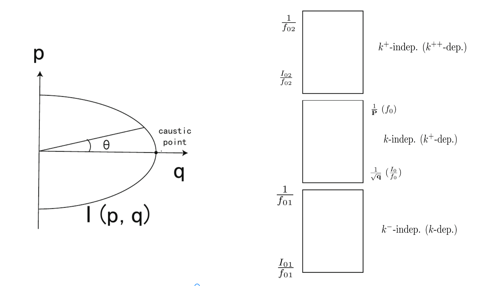
Figure 12: (Left) Schematic diagram for the phase space where $I({\bf p},{\bf q})$ is a classical action. (Right) The segments for the method CALP where $k$ is the variable in centroid here.

In the integrable side, the selection of classical actions leads to the averaged results[4]

$$\overline{V(q+\frac{r_{i}}{2})V^{*}(q-\frac{r_{i}}{2})}=\frac{\delta(E-{\bf p}^{2}-{\bf q})}{\int d{\bf q}\int d{\bf p}\delta(E-{\bf p}^{2}-{\bf q})},$$ (54)

$$\overline{|V(q)|^{2}}=\frac{\int d{\bf p}\delta(E-{\bf p}^{2}-{\bf q})}{\int d{\bf q}\int d{\bf p}\delta(E-{\bf p}^{2}-{\bf q})}=\frac{(E-{\bf q})^{\eta}}{\int d{\bf q}(E-{\bf q})^{\eta}},$$

where $\eta=\frac{-1}{2}$ in the caustics point, and $\eta=0$ in other points locate in the integrable region. As shown in Fig.12, in the systems where integrability is dominant, the length of ${\bf p}$ is very small, which has very simple expression $|{\bf p}|=\sqrt{E-{\bf q}}$, in aid of the selection of the actions through the $n$-dimensional delta function, where here $n$ is the number of distinct good quantum numbers, which is also the number of local sites that participate in the average calculation here.

Specifically, near the caustic point, we have the following relation

$${\bf p}^{2}={\bf q}[{\bf p}],$$ (55)

i.e., the squared ${\bf p}$ can be replaced by the ${\bf q}[{\bf p}]$ as a functional of ${\bf p}$, and the caustic point satisfies

$${\bf q}[{\bf p}]={\bf p}[0]={\bf p},$$ (56)

$$\frac{{\bf q}}{{\bf p}}=0,$$

which indicate the special property when near the caustic point of a torus, i.e., the large variance of $\frac{d\boldsymbol{\theta}}{d{\bf q}}$ in terms of the angle as shown in Fig.12. Also, we can know that $E$ can be approximated as $2{\bf q}$ in this case.

Moreover, at the caustic point with $\eta=-1/2$, the numerator and denorminator of the above local average function satisfies

$$\int d{\bf p}\delta(E-{\bf p}^{2}-{\bf q})=\sum_{i}{\bf p}_{i}=\frac{1}{{\bf p}}=\frac{1}{\sqrt{{\bf q}[{\bf p}]}},$$ (57)

$$\int d{\bf q}\int d{\bf p}\delta(E-{\bf p}^{2}-{\bf q})=\int d{\bf q}\ {\bf q}^{-1/2}=1.$$

We will mainly using this formula, which is for the ergodic system with stochastic classical motions and the influence of different ${\bf p}$ on the functional ${\bf q}[{\bf p}]$ are uncorrelated, which make sure that the summation over the discrete samples ${\bf p}_{i}$ are solely for a symmetry sector where each one are selected by the delta function.

Thus in this case the second moment of perturbation is

$$\overline{|V(q)|^{2}}=\frac{1}{\sqrt{{\bf q}[{\bf p}]}}=\frac{1}{{\bf p}},$$ (58)

which turns to infinite due to the vanishing length of ${\bf p}$. In the above ergodic-type expressions for the averaged Wigner function, the selection of delta-function takes effect, but in the mean time the selection results in a special configuration that the local and nonlocal conservations coexist. This will be explained below section, in terms of the infinite series over the discrete samples selected (or filtered) by the delta functions that depending on the overlap (or classical analog) between the classical energy surface and the classical actions, where nonlocal conservations are perserved by the selections (in the same pattern) and form a certain symmetry sector. In the integrable system, such nonlocal conservation is dominant, in comparasion to the Gaussian randomness which is brought by the local conservation and related to the non-negligible effect of integrable eigenstate fluctuation.

5.1 Usage of correlations of the adjacent local points (CALP)

Next we introduce an analytical method where we present more details in Appendix.A and Supplemental material. This method is base on the estimation of the correlations of the adjacent local points (CALP), where the nearby local points form a continuum and conserved observation, whose nonlocal symmetry properties can be projected to the invariant microcanonical averages within the narrow microcanonical intervals formed by the scaled variables.

When the system is in the integrable and nonergodic side, where the characteristic de Broglie wavelength is much larger than the integrable state’s fluctuation, we use an analysis expression to represent the projection ${\bf p}$,

$$\frac{1}{{\bf p}}=\lim_{k\rightarrow\infty}\sum_{\gamma=0}^{k-1}\left(\frac{1}{z}\right)^{\gamma}=\frac{z}{z-1},$$ (59)

while the quantity ${\bf q}$ can be expressed as

$$\frac{1}{\sqrt{{\bf q}}}=\frac{I_{0}}{f_{0}}=1-\frac{1}{\partial_{k^{+}}f_{0}}.$$ (60)

Note that the method CALP used here requires the definition of the following quantities, where more details are presented in Appendix.A,

$$f_{0}=\frac{1}{{\bf p}},$$ (61)

$$I_{0}=f_{0}\frac{\partial_{k^{+}}f_{0}-1}{\partial_{k^{+}}f_{0}}.$$

Equivalently, in terms of such discrete summations there is, according to the Berry conjecture, another equivalent expression for $\overline{|V(q)|^{2}}$ which is more nonergodic-type, but also scales to infinite in the caustic point just like the above expression[4],

$$\overline{|V(q)|^{2}}=\delta({\bf I}({\bf p},{\bf q})-{\bf I}_{n}),$$ (62)

where ${\bf I}_{n}$ is the local average of the actions corresponding to the pathological nonergodic classical motions in the phase space, and each ${\bf I}_{n}$ corresponds to a good quantum number that plays the role of the power of integrable state generator. Using the property of delta-function $\delta(f(x))=\sum_{i}\frac{\delta(x-x_{i})}{|\partial_{x}f(x)|}$, with $x_{i}$ are roots of $f(x)$, we obtain

$$\overline{|V(q)|^{2}}=\frac{1}{\sqrt{{\bf q}}}=\frac{I_{0}}{f_{0}}=\sum_{ki}\left|\frac{d{\bf I}({\bf q},{\bf p}_{ki})}{d{\bf p}}\right|^{-1}=\sum_{i}\left|\frac{d\boldsymbol{\theta}({\bf q},{\bf p}_{i})}{d{\bf q}}\right|=\frac{\partial_{k^{+}}f_{0}-1}{\partial_{k^{+}}f_{0}},$$ (63)

where the differentials are related to the local quantities through

$$\left[\sum_{i}\left|\frac{d\boldsymbol{\theta}({\bf q},{\bf p}_{ki})}{d{\bf q}}\right|\right]^{-1}=\sum_{\gamma=0}^{\infty}\left(\frac{1}{\partial_{k^{+}}f_{0}}\right)^{\gamma},$$ (64)

$$\sum_{i}\left|\frac{d{\bf I}({\bf q},{\bf p}_{i})}{d{\bf p}}\right|^{-1}=\sum_{i=1}^{\infty}\left(1-\frac{f_{0}}{I_{0}}\right)^{i-1},$$

where we also have

$$\sum_{i}\left|\frac{d\boldsymbol{\theta}({\bf q},{\bf p}_{i})}{d{\bf q}}\right|=\left|\frac{d\sum_{i}\boldsymbol{\theta}({\bf q},{\bf p}_{i})}{d{\bf q}}\right|=\frac{\partial_{k^{+}}f_{0}-1}{\partial_{k^{+}}f_{0}}=\left[\partial_{k}(I_{0}-f_{0})\right]^{-1},$$ (65)

$$\sum_{ki}\left|\frac{d{\bf I}({\bf q},{\bf p}_{ki})}{d{\bf p}}\right|=\sum_{i=1}^{\infty}\left(\frac{I_{0}}{I_{0}-f_{0}}\right)^{i-1}=\sum_{i=1}^{\infty}\left(1-\partial_{k^{+}}f_{0}\right)^{i-1},$$

and through the sampling rule for the indices of ${\bf p}$ in the summation, we can obtain

$$\frac{d{\bf I}({\bf q},{\bf p}_{ki})}{d{\bf p}}=\partial_{k^{+}}f_{0},$$ (66)

$$\left|\frac{d\boldsymbol{\theta}({\bf q},{\bf p}_{i})}{d{\bf q}}\right|=\frac{f_{0}}{I_{0}}=\frac{\partial_{k^{+}}f_{0}}{\partial_{k^{+}}f_{0}-1},$$

where the first expression is deduced in Appendix.B. Here, for convenience of analytical analysis, we define $\frac{1}{{\bf p}}=\frac{z}{z-1}$ with $z$ a positive real integer (for more details see Appendix.A). Here we use another infinite quantity in caustic point $\frac{1}{\sqrt{{\bf q}}}$ instead of $\frac{1}{{\bf p}}$, and in fact these two quantities has minor difference even in caustic point, as discussed in below section; While for the second expression, in comparasion with Eq.(LABEL:4277), we obtain

$$\frac{d\sum_{i}\boldsymbol{\theta}({\bf q},{\bf p}_{i})}{d\boldsymbol{\theta}({\bf q},{\bf p}_{i})}=\frac{I_{0}^{2}}{f_{0}^{2}}=\left[\partial_{k}(I_{0}-f_{0})\right]^{-2}=I_{0}\partial_{k^{+}}\frac{I_{0}}{f_{0}}.$$ (67)

In the first line of Eq.(LABEL:4251) the selection of delta function results in the summation over the local sites labeled by $i$, and we have the following expressions,

$$\sum_{i}{\bf p}_{i}=\sum_{i}{\bf p}_{i}[{\bf q}]=\sum_{i=1}^{\infty}(1-p)^{i-1}=\sum_{i=1}^{\infty}\left(\frac{1}{z}\right)^{i-1}=\frac{z}{z-1}=\frac{1}{{\bf p}}.$$ (68)

Then in the integrable side, the averaged Wigner function in the first line of Eq.(LABEL:511) can be rewriten as

$$\overline{V(q+\frac{r_{i}}{2})V^{*}(q-\frac{r_{i}}{2})}=\delta(E-{\bf p}^{2}-{\bf q})=\partial_{i}\left[\frac{1}{{\bf p}}\right]_{i}\approx\partial_{k^{+}}{\bf I}[{\bf p}+k^{+}],$$ (69)

which corresponds to the maximal derivative of the classical action ${\bf I}[{\bf p}+k^{+}]$ on $k^{+}$. Here we built a correspondence between the delta-function representation and the functional expansion of the classical action (which is the $\frac{1}{{\bf p}}$ here), where we present the details in Appendix.A, Appendix.B, and the Supplemental material. As we shown in Appendix.A, as the $\frac{1}{{\bf p}}$ increase to an largest extend, and nearly reaches the upper boundary of the $k^{+}$-independent segment, which is represented by the functional ${\bf I}[{\bf p}]$, its dependence on $k^{+}$ is vanishingly small, in which occasion we can expand the $k^{+}$-dependence of $\frac{1}{{\bf p}}$ in terms of the derivatives of the delta-type function in a series of order (as we shown in Appendix.A) and such correspondence is being further verified in terms of the second set of CALP as we shown in Sec.C in Supplemental material, where the dominant nonlocal effect smoothing the difference (and independence) between different segments. Then, in terms of teh method of CALP, the result in the seond line of Eq.(LABEL:4251) can be rewritten as

$$\int d{\bf q}\int d{\bf p}\delta(E-{\bf p}^{2}-{\bf q})=\sum_{i}\left[\frac{I_{0}}{f_{0}}\right]_{i}=1,$$ (70)

where the summation is over the discrete local points that are selected according to the rule of minimal local-variable-dependence, which is, inother word, maximal nonlocal chanracter. This can also be verified using the fnctional derivatives of the classical action with their corresponding variable as shown in Appendix.B

Importantly, here the classical analog between $f_{0}$ and $\frac{1}{\sqrt{{\bf q}}}=\frac{I_{0}}{f_{0}}$ originates from the their same derivatives with respect to $k$, which is the variable in one of the local points. In this perspective, we can further define the $f_{0}$ in terms of an identity whose functional summation (which is indeed the integral containing selections by the delta function) is equivalents to taking the limit on the variable $k^{+}$ (with smaller variation than $k$), and in the mean time, remove the $k^{+}$-dependence on $f_{0}$ through the homogenization on the averaged Wigner function with the local averaged one,

$$1_{k^{+}}=\delta(\partial_{k}\frac{I_{0}}{f_{0}})=\sum_{p_{0}}e^{-ip_{0}r_{i0}}\overline{\sum_{i_{0}}e^{ip_{0}r_{i_{0}}}\left[\frac{1}{N}\left(w_{i}(\frac{r_{i0}}{2})F[k^{+}]+w_{i}(-\frac{r_{i0}}{2})(1-F[k^{+}])\right)\right]},$$ (71)

where $p_{0},\ i_{0}$ denote the projection and integrable state fluctuation in this subsystem, and $w_{i}$ is the weight which leads to the finite $k^{+}$-dependence on the identity $1_{k^{+}}$. $F[k^{+}]$ is an arbitary functional of $k^{+}$. Note that in terms of a number one with finite $k^{+}$-dependence, it all refers to the $\frac{1}{{\bf p}}$, until we using the notation $\frac{I_{0}}{f_{0}}$ which refers to the $\frac{1}{\sqrt{{\bf q}}}$, and the delta function of $\partial_{k}\frac{I_{0}}{f_{0}}$ in second term of above expression is only to indicate such common $k$-independent feature which is shared by both the $\frac{1}{{\bf p}}$ and $\frac{1}{\sqrt{{\bf q}}}$. The homogenization process is equivalents to making the Berry autocorrelation be one in this subsystem, i.e.,

$$\sum_{i_{1}}[1_{k^{+}}]_{i_{1}} =\sum_{p_{0}}e^{-ip_{0}r_{i0}}\underline{\sum_{i,i_{0}}e^{ip_{0}r_{i0}}\left[\frac{1}{N}(w_{i}(\frac{r_{i0}}{2})F[k^{+}]+w_{i}(-\frac{r_{i0}}{2})(1-F[k^{+}]))\right]}$$ (72)

$$\approx\sum_{p_{0}}\sum_{i,i_{0}}e^{ip_{0}r_{i0}}\left[\frac{1}{N}(w_{i}(\frac{r_{i0}}{2})F[k^{+}]+w_{i}(-\frac{r_{i0}}{2})(1-F[k^{+}]))\right]$$

$$=\overline{\left[\sum_{i}\frac{1}{N}\left(w_{i}(0)F[k^{+}]+w_{i}(0)(1-F[k^{+}])\right)\right]}=1,$$

where the summation over $p_{0}$ on the term with bottom line, i.e.,

$$\sum_{p_{0}}\underline{\sum_{i,i_{0}}e^{ip_{0}r_{i0}}\left[\frac{1}{N}(w_{i}(\frac{r_{i0}}{2})F[k^{+}]+w_{i}(-\frac{r_{i0}}{2})(1-F[k^{+}]))\right]},$$ (73)

can be viewed as a local average over the $k^{+}$-dependent region, similar to the classical action ${\bf I}[{\bf p}+k^{+}]$ in Eq.(142), and as system closes to the integrable side, which means the above local averaged term becomes very large and the summation turns to the selective one over the discrete terms following the same pattern (see Eq.(LABEL:4285)), and in the mean time, the derivative of such local averaged term becomes vanishingly small, and the nonlocal correlations between the adjacent regions (or segments) become overwhelming that the local correlations inside the single segment. Thus the $p_{0}$ (within the term $e^{-ip_{0}r_{i0}}$) is, quite reasonablely, vanishingly small due to the selection effect, and now the above averaged Wigner function becomes the same with the local average density function, where the effect of $r_{i0}$ has being smoothed out by the average. Here the summation over $i_{1}$ corresponds to taking the limit $k^{+}\rightarrow\infty$. Note that the result in Eq.(72), which is one, indeed does not directly reflect the quantitative value of the local averaged function itself, but in terms of the variable of the next segment $k^{+}$, as a result of the large fluctuation in the boundaries, which leads to more nonlocal correlation, and less locally distinctive features (see Appendix.B for an example). We also note that, what we mean by large integrable eigenstate fluctuation here, counterintuitively, corresponds to less effect from the boundary exchanging term $r_{i0}$, after the average in the last line of Eq.(72). This is because the $r_{i0}$ term here does not represents the oscillator amplitude which is inversely proportional to the number of local oscillators (and thus also to the nonlocal correlation). While here the large fluctuation of boundary exchanging term $r_{i0}$ is related to the low dimensional condition as shown in Eq.(LABEL:511) where $\eta=-1/2=\frac{d}{2}-1$ corresponds to the effective dimension $d=1$ here, and the large fluctuation leads to smaller variance as well as the enhanced homogenization between the adjacent segments, where the individual characteristics of different segments fade to some extent.

Now we have the smoothed version of $1_{k^{+}}(=\frac{1}{{\bf p}})$, which we express it using $z^{\prime}$,

$$\sum_{i_{1}}[1]_{i_{1}}=\frac{z^{\prime}}{z^{\prime}-1}\sum_{i_{2}}[1-\left(\frac{1}{z^{\prime}}\right)^{k^{+}}]_{i_{2}}=\frac{z^{\prime}}{z^{\prime}-1},$$ (74)

and thus $f_{0}=\sum^{k^{+}-1}_{\gamma=0}\left(\frac{1}{z^{\prime}}\right)^{\gamma}$. Here the summation over $i_{2}$ represents taking the limit $k^{+}\rightarrow\infty$ for the part within the bracket, which is indeed the fluctuation from the lower boundary of the upper segment into the current $k^{+}$-dependent segment. The the identity embeded in the above expression satisfies

$$\sum_{i_{2}}[1-\left(\frac{1}{z^{\prime}}\right)^{k^{+}}]_{i_{2}}=1.$$ (75)

This is a very important result, and we will explain it latter.

Note that $z^{\prime}\neq z$, otherwise $\lim_{k^{+}\rightarrow\infty}f_{0}=f_{0}$. Also, we have the expression

$$\lim_{k^{+}\rightarrow\infty}f_{0}=\lim_{k^{+}\rightarrow\infty}(\lim_{k\rightarrow\infty}f_{1})=\frac{f_{0}}{1-\left(\frac{1}{z^{\prime}}\right)^{k^{+}}}=\frac{z^{\prime}}{z^{\prime}-1},$$ (76)

where the derivative of $f_{0}$ with respect to $k^{+}$ is $\partial_{k^{+}}f_{0}=\frac{(\partial_{k}f_{1})^{2}}{\partial_{k}f_{1}-1}$ (see Appendix.A). $f_{1}=\sum^{k-1}_{\gamma=0}\left(\frac{1}{z}\right)^{\gamma}$ is the generator of $f_{0}$, and we can obtain $f_{0}$ by smooth out the $k$-dependence on $f_{1}$, $f_{0}=\lim_{k\rightarrow\infty}f_{1}$.

Thus more precisely, the difference between $\frac{1}{{\bf p}}$ and $\frac{1}{\sqrt{{\bf q}}}$ is that they identify the upper boundary and lower boundary of the region where can be estimated as that the $k$-dependence has being smoothed out, that is to say,

$$\partial_{k^{+}}\frac{1}{{\bf p}}\neq 0,$$ (77)

$$\partial_{k^{+}}(\frac{1}{{\bf p}}+0^{+})=0,$$

$$\partial_{k}\frac{1}{\sqrt{{\bf q}}}=0,$$

$$\partial_{k}(\frac{1}{\sqrt{{\bf q}}}-0^{-})\neq 0.$$

Thus to make sure $\frac{1}{{\bf p}}$ and $\frac{1}{\sqrt{{\bf q}}}$ are locate in the correct boundaries of the $k$-independent region, we make an important assumption for the terms in Eq.(75), i.e.,

$$\left(\frac{1}{z^{\prime}}\right)^{k^{+}}=\frac{1}{\partial_{k^{++}}(I_{0}-f_{0})}=\partial_{k^{+}}f_{0}=0,$$ (78)

where we use the formula presented in Appendix.A, $\partial_{k^{++}}(I_{0}-f_{0})=\frac{1}{\partial_{k^{+}}f_{0}}$, thus the approximation at the boundary $\partial_{k^{+}}f_{0}\approx 0$ is equivalents to the $\partial_{k^{++}}(I_{0}-f_{0})=\infty$. The above equility guarantees we can correctly identify the lower boundary of the $k^{++}$-independent segment which is the $\frac{I_{02}}{f_{02}}$ (see Appendix.A). In the mean time, as we discuss in Appendix.A, when we set $\partial_{k^{+}}f_{0}=\left(\frac{1}{z^{\prime}}\right)^{k^{+}}$ is nearly zero, the corresponding $k^{+}$-dependent term $(1-\left(\frac{1}{z^{\prime}}\right)^{k^{+}})$ now indeed represent the largest possible fluctuation of the lower boundary of $k^{+}$-independent segment ($\frac{I_{02}}{f_{02}}$) into the $k$-independent segment, and the summation over $i_{2}$ remove such fluctuation-induced $k$-dependence. When such $k$-dependence of the lower boundary of upper segment is completely removed (after the local average on a certain boundary), the random fluctuations play no role and the perturbations are deviated from random Guassian function, and the Wigner average reduces to the local average and results in the Berry antocorrelation $\mathcal{C}$ be nearly one, which also corresponds to the maximized IPR (corresponds to the many-body localization phase). Note that for arbitarily two adjacent segments, the fluctuations of the lower boundary of upper segment and that of the upper boundary of the lower segment are mutually correlated, just like the integrable eigenstate fluctuations represented by $\pm\frac{r_{i}}{2}$ in Eq.(51).

Also, we note that $\frac{I_{02}}{f_{02}}$ is related to the lower boundary of the $k$-independent segment by $\frac{I_{02}}{f_{02}}=\lim_{k^{+}\rightarrow\infty}\frac{1}{\sqrt{{\bf q}}}=\lim_{k^{+}\rightarrow\infty}\frac{I_{0}}{f_{0}}$.

The summation over $i_{2}$ reads

$$\sum_{i_{2}}[1-\left(\frac{1}{z^{\prime}}\right)^{k^{+}}]_{i_{2}}=\sum_{i_{2}}[1-O(\partial_{k^{+}}f_{0}+0^{+})]_{i_{2}}=\sum_{i_{2}}[1]_{i_{2}}=\frac{I_{02}}{f_{02}},$$ (79)

where the $[1]_{i_{2}}$ here is the lower boundary of the $k^{+}$-independent segment but being endowed the maximal $k^{+}$-dependence through the fluctuation. Assuming such largest fluctuation is possible to reaches the bottom of the lower segment (see Appendix.A), then $\frac{I_{02}}{f_{02}}$ should shares the feature of $\frac{I_{0}}{f_{0}}$, and the summation over $i_{2}$ is then similar to Eq.(71,72).

Following the same pattern due to the nonlocal symmetry, for $k^{-}$-independent segment, which is below the $k$-independent one, the quantity in bottom of $k^{-}$-independent segment reads

$$1_{k}=\delta(\partial_{k^{-}}\frac{I_{01}}{f_{01}})=\sum_{p_{01}}e^{-ip_{01}r_{i01}}\overline{\sum_{i_{01}}e^{ip_{01}r_{i01}}\left[\frac{1}{N}(w_{i}(\frac{r_{i01}}{2})F[k]+w_{i}(-\frac{r_{i01}}{2})(1-F[k]))\right]},$$ (80)

where $r_{i01}$ represents the the smoothing process for the $k$-dependence can be expressed as

$$\sum_{i_{1}}[1]_{i_{1}} \approx\sum_{p_{01}}\sum_{i,i_{01}}e^{ip_{01}r_{i01}}\left[\frac{1}{N}(w_{i}(\frac{r_{i01}}{2})F[k]+w_{i}(-\frac{r_{i01}}{2})(1-F[k]))\right]$$ (81)

$$=\overline{\left[\sum_{i}\frac{1}{N}(w_{i}(0)F[k]+w_{i}(0)(1-F[k]))\right]}=\frac{I_{01}-f_{01}}{\frac{I_{01}}{f_{01}}}$$

$$=\frac{f_{01}}{1-\partial_{k}f_{01}}\sum_{i_{3}}\left[1-\partial_{k}f_{01}\right]_{i_{3}}=\frac{f_{01}}{1-\partial_{k}f_{01}}=\frac{I_{0}}{f_{0}},$$

where

$$I_{01}-f_{01}=\frac{-f_{01}}{\partial_{k}f_{01}},$$ (82)

$$\frac{I_{01}}{f_{01}}=\frac{\partial_{k}f_{01}-1}{\partial_{k}f_{01}},$$

and, still, the summation over $i_{3}$ correspond to smoothing of the $k^{-}$-dependence, where $\sum_{i_{3}}\left[1\right]_{i_{3}}=\frac{I_{01}}{f_{01}}$ is the lower boundary of the $k^{-}$-independent region, with $\partial_{k}(f_{01}+0^{+})=0$.

6 Level statistic for GOE and GUE

In terms of the GOE system consider in above content, we show in Figs.13 and Fig.14 the eigenvalue distribution and the level statistic, where the simulations show $\langle r\rangle=0.54$, $\langle\tilde{r}\rangle=1.76$. There may exist the symmstry-protected topological order, where the the many-body levels are nondegenerate only when the corresponding quantum number be the multiple of the number of cetrain fermion mode species (which is related to the corresponding nonlocal conservation sector). As we mention above, even for a system in ETH phase, as long as there exist the nonlocal symmetry sectors which generate different symmetry parities, the spectrum need to be considered seperetely in each sector. In this case, the boundary degenerated zero modes can be protected by the nontrivial topological order in the bulk (against the interaction effects), and during the smulation of level statistic, the degenerate part of the specrum can be filted in terms of the criterion of a certain definite symmetry parity sector.

Figure 13: Eigenvalues and products in GOE.

Figure 14: Level statistic of GOE.

Figure 15: Eigenvalues and products in GUE.

Figure 16: Level statistic of GUE.

We can consider an additional Chiral symmetry into the GOE system and breaks the time reversal symmetry. This is realized in terms of some statistical conservation which corresponds to some sort of symmetry pattern as exhibited from the moments of higher order. As shown in the below simulations, the chaostic effect can be seem as far as we sample $N$ distinct elements (indiscriminately) from a $N\times N$ GOE matrix, which may containing degeneracies as can be seem through exact diagonalization. But if the samples amount is much larger that $N$, the many-body localization as well as the Poission distribution will be inevitable.

This can be represented by an additional symmetry sector (or two symmetry blocks) in the resulting complex Gaussian random matrix. The absence of $\mathcal{T}$-invariance here can also be described by the degenerated boundary zero mode protected by the quantum order of the bulk part that is generated by the symmetry and in terms of a complex fermion mode species whose periodicity is half of the GOE one, and the distinct periodicities of GUE and GOE can be represented by two adjacent Fibonacci numbers. In Figs.15 and Fig.16, we show a level statistic simulation, where we choose a set of distinct positive eigenvalues arranged in ascending order, and the GUE characteristic can be verified in terms of the diagonalizable matrices. The simulations show $\langle r\rangle=0.604$, $\langle\tilde{r}\rangle=1.342$.

7 Conclusion

We propose a method to construting the commensurate eigenvector basis that are appropriate for the numerical calculation as well as the diagonal or off-diagonal ETH diagnostics. We also investigate the integrablity-chaos transition with independent perturbations in terms of the Berry autocorrelation in semicalssical limit, where there is a phase space spanned by the momentum-like projection and the range of local wave function. We also develop a method, CALP, to investigate the integrablity-chaos transition. in the presence of uncorrelated peturbations and correlated integrable eigenstate fluctuations, which is applicable for both the ergodic and nonergodic systems. More importantly,this work reveals and illustrates to a certain extent the essential role of the Golden ratio and the constant $\frac{1}{3}$ in the quantum chaos physics.

8 Appendix.A: Simulation of GOE

The target random matrix is base on a Hermitian operator $\hat{H}$, whose eigenkets are sampled from the elements of the known GOE matrix. Here we write the matrix elements as

$$H_{mn}=\langle m|\hat{H}|n\rangle=\sum_{i}\lambda_{i}(\psi_{m})^{*}\psi_{n},$$ (83)

where $\lambda_{i}$ denotes its eigenvalues $\hat{H}|i\rangle=\lambda_{i}|i\rangle$, and $(\psi_{m})^{*},\psi_{n}$ are the eigenvectors selected by the eigenkets. For simplicity, we consider these are only two eigenvalues $a_{1}$ and $a_{2}$, and not necessarily have $a_{1}=-a_{2}$ in this step.

In terms of the orthogonal transformation of the GOE matrix, we can rewrite the $N\times N$ ($m,n=1,2,\cdots,N$) sample GOE matrix in Appendix.A in the following simple $2\times 2$ form, which is valid in considering the thermalization of the diagonal elements but has side-effect during considering the off-diagonal ones, as will be explained below.

$${\bf O} ={\bf Q}^{T}{\bf O}_{i}{\bf Q}$$ (84)

$$=\begin{pmatrix}{\rm cos}\theta&-{\rm sin}\theta\\ {\rm sin}\theta&{\rm cos}\theta\end{pmatrix}^{T}\begin{pmatrix}a_{1}&0\\ 0&a_{2}\end{pmatrix}\begin{pmatrix}{\rm cos}\theta&-{\rm sin}\theta\\ {\rm sin}\theta&{\rm cos}\theta\end{pmatrix},$$

where the ${\bf O}_{i}$ is the diagonal matrix of eigenvalues, and ${\bf Q}$ in the rightside of ${\bf O}_{i}$ is the orthogonal matrix whose first and second rows correspond to the eigenvectors of the eigenvalues $a_{2}$ and $a_{1}$, respectively. This is to make sure average over eigenkets $|m\rangle$ has $\overline{|\psi_{i}^{m}|}=0$ as will be shown below. Then we have the symmetry $2\times 2$ matrix

$${\bf O} =\frac{2}{\sqrt{a_{1}^{2}+a_{2}^{2}}}\begin{pmatrix}a_{1}{\rm cos}^{2}\theta+a_{2}{\rm sin}^{2}\theta&(-a_{1}+a_{2}){\rm cos}\theta{\rm sin}\theta\\ (-a_{1}+a_{2}){\rm cos}\theta{\rm sin}\theta&a_{2}{\rm cos}^{2}\theta+a_{1}{\rm sin}^{2}\theta\end{pmatrix},$$ (85)

whose four elements have the zero mean and unit variance the same with $\overline{O_{mn}}$ (thus here we use the same notation). The diagonal elements have zero mean and variance equals to 2, $\overline{O_{mn}}=\frac{a_{1}+a_{2}}{\sqrt{a_{1}+a_{2}}}=0$, $\overline{O^{2}_{2\times 2}}=\frac{(a_{1}-a_{2})^{2}{\rm cos}^{2}(2\theta)}{a_{1}^{2}+a_{2}^{2}}=2$. It is important to note that, a difference between the matrix ${\bf O}$ (in dimension-reduced form) and ${\bf H}_{mn}$ generated by it, is that in GOE matrix ${\bf O}_{mn}$, $a_{1}=-a_{2}$ and $\theta=\pi/2$. These two conditions are required to ensure the Gaussian distribution. But in ${\bf H}$, these conditions are not required, as can be seem below, although we use the same notation for the eigenvalues here, there are indeed two parts of eigenvalues in ${\bf H}$ during the analysis of its thermalization: part of eigenvalue $a_{1}$ satisfies $a_{1}=-a_{2}$ while others are not needed at least before its distributions are known, and the other eigenvalue $a_{2}$ is the same.

Then the target matrix generated by it can be obtained by adding the mean value of eigenvalues in the diagonal positions (which not need to be zero now as they can be treated as arbitarily two eigenvalues in a many-body spectrum),

$${\bf H} =\delta_{mn}\frac{a_{1}+a_{2}}{2}+\frac{\sqrt{a_{1}^{2}+a_{2}^{2}}}{2}O_{mn} =\begin{pmatrix}\frac{a_{1}+a_{2}}{2}+a_{1}^{2}{\rm cos}^{2}\theta+a_{2}^{2}{\rm sin}^{2}\theta&(-a_{1}+a_{2}){\rm cos}\theta{\rm sin}\theta\\ (-a_{1}+a_{2}){\rm cos}\theta{\rm sin}\theta&\frac{a_{1}+a_{2}}{2}+a_{2}^{2}{\rm cos}^{2}\theta+a_{1}^{2}{\rm sin}^{2}\theta\end{pmatrix}.$$ (86)

It can be seem that, in diagonal positions, the second terms containing the $\theta$ describe the instability. This is the same with teh case in off-diagonal positions, however, to analysis the instability there, $\theta$ cannot be simple $\pi/2$ since the symmetry property requires the two off-diagonal elements be the same and have zero mean in the same time, thus the two off-diagonal elements are both zero and own null variance.

Next, under the preserved normalization condition for the eigenvalues, we introduce another set of eigenvectors (for eigenvalues $i$ and $j$ representing the $a_{1}$ and $a_{2}$, respectively) to including the part related to the fluctuations

$$\psi_{i}^{m}=\frac{1}{2}\begin{pmatrix}\cos\theta\\ \sin\theta\\ \cos\theta\\ \cos\theta\end{pmatrix},\psi_{i}^{m^{\prime}}=\frac{1}{2}\begin{pmatrix}\cos\theta\\ \sin\theta\\ -\cos\theta\\ -\cos\theta\end{pmatrix},\psi_{i}^{n}=\frac{1}{2}\begin{pmatrix}-\sin\theta\\ -\cos\theta\\ -\sin\theta\\ -\sin\theta\end{pmatrix},\psi_{i}^{n^{\prime}}=\frac{1}{2}\begin{pmatrix}-\sin\theta\\ -\cos\theta\\ \sin\theta\\ \sin\theta\end{pmatrix},$$ (87)

$$\psi_{j}^{m}=\frac{1}{2}\begin{pmatrix}\sin\theta\\ -\cos\theta\\ \sin\theta\\ \sin\theta\end{pmatrix},\psi_{j}^{m^{\prime}}=\frac{1}{2}\begin{pmatrix}\sin\theta\\ -\cos\theta\\ -\sin\theta\\ -\sin\theta\end{pmatrix},\psi_{j}^{n}=\frac{1}{2}\begin{pmatrix}\cos\theta\\ -\sin\theta\\ \cos\theta\\ \cos\theta\end{pmatrix},\psi_{j}^{n^{\prime}}=\frac{1}{2}\begin{pmatrix}\cos\theta\\ -\sin\theta\\ -\cos\theta\\ -\cos\theta\end{pmatrix},$$

where there are four elements in each eigenvector instead of just two and the last two elements correspond to the fluctuation part of diagonal component, and the requirement of zero mean for each Gaussian distributed eigenvector produces another eigenvectors $\psi_{i}^{m^{\prime}}$ and $\psi_{i}^{n^{\prime}}$ in addition to the $\psi_{i}^{m}$ and $\psi_{i}^{n}$. Here these two eigenvectors satisfy $|\psi_{i}^{m}|^{2}=|\psi_{i}^{m^{\prime}}|^{2}$, $|\psi_{i}^{n}|^{2}=|\psi_{i}^{n^{\prime}}|^{2}$. As these two eigenvectors describe the fluctuation part of diagonal elements, they should be viewed as of the same category when multipiled by the eigenvalues, thus the diagonal elements can be expressed as

$$H_{mm} =a_{1}(|\psi_{i}^{m}|^{2}+|\psi_{i}^{m^{\prime}}|^{2})+a_{2}(|\psi_{j}^{m}|^{2}+|\psi_{j}^{m^{\prime}}|^{2})$$ (88)

$$=a_{1}(\frac{1}{2}+\cos^{2}\theta)+a_{2}(\frac{1}{2}+\sin^{2}\theta),$$

$$H_{nn} =a_{1}(|\psi_{i}^{n}|^{2}+|\psi_{i}^{n^{\prime}}|^{2})+a_{2}(|\psi_{j}^{n}|^{2}+|\psi_{j}^{n^{\prime}}|^{2})$$

$$=a_{1}(\frac{1}{2}+\sin^{2}\theta)+a_{2}(\frac{1}{2}+\cos^{2}\theta),$$

whose average over the eigenkets is

$$\overline{H_{mm}}=\frac{1}{d}(a_{1}+a_{2}),$$ (89)

where $\frac{1}{d}$ is the variance of the eigenvectors, $\overline{(\psi_{i}^{m})^{*}\psi_{j}^{n}}=\overline{|\psi_{i}^{m}|^{2}}=\frac{1}{d}\delta_{mn}\delta_{ij}$, where $d$ is the dimension of the Hilbert space and $d=2$ here labeling the flavors of the eigenkets, and this variance a precondition we get the valid samples from the GOE random Gaussian matrix. In other word, the behaviors (moments of distribution) of $\psi_{i}^{m}$ determine the distribution of the elements in target matrix ${\bf H}$. While the off-diagonal elements of ${\bf H}$ can be obtained

$$H_{mn}=H_{nm} =\frac{1}{4}a_{1}\left[(\psi_{i}^{m})^{*}\psi_{i}^{n}+(\psi_{i}^{m^{\prime}})^{*}\psi_{i}^{n^{\prime}}+(\psi_{i}^{m})^{*}\psi_{i}^{n^{\prime}}+(\psi_{i}^{m^{\prime}})^{*}\psi_{i}^{n}\right]$$ (90)

$$+\frac{1}{4}a_{2}\left[(\psi_{j}^{m})^{*}\psi_{j}^{n}+(\psi_{j}^{m^{\prime}})^{*}\psi_{j}^{n^{\prime}}+(\psi_{j}^{m})^{*}\psi_{j}^{n^{\prime}}+(\psi_{j}^{m^{\prime}})^{*}\psi_{j}^{n}\right]=(-a_{1}+a_{2})\cos\theta\sin\theta.$$

The variance of the diagonal elements for GOE reads $\overline{H_{mm}^{2}}-\overline{H_{mm}}^{2}$ where each term satisfies

$$\overline{H_{mm}^{2}}=\frac{H_{mm}^{2}+H_{nn}^{2}}{2}=(a_{1}^{2}+a_{2}^{2})\overline{|\psi_{i}^{m}|^{4}}+2a_{1}a_{2}\overline{|\psi_{i}^{m}|^{2}|\psi_{j}^{m}|^{2}},$$ (91)

$$\overline{H_{mm}}^{2}=(a_{1}^{2}+a_{2}^{2})(\overline{|\psi_{i}^{m}|^{2}})^{2}+2a_{1}a_{2}(\overline{|\psi_{i}^{m}|^{2}})(\overline{|\psi_{j}^{m}|^{2}}).$$

As we consider the simplized configuration with $d=2$, we have $(\overline{|\psi_{i}^{m}|^{2}})(\overline{|\psi_{j}^{m}|^{2}})=\overline{|\psi_{i}^{m}|^{2}|\psi_{j}^{m}|^{2}}=\frac{1}{4}$.

Then let us look back to the expression of the diagonal elements in Eq.(90), whose mean value and variance

$$\overline{H_{mm}}=\frac{H_{mm}+H_{nn}}{2}=a_{1}+a_{2},$$ (92)

$$\overline{H_{mm}^{2}}=\frac{H_{mm}^{2}+H_{nn}^{2}}{2}=\frac{1}{4}(a_{1}-a_{2})^{2}\cos^{2}(2\theta)=\frac{1}{4}(a_{1}-a_{2})^{2},$$

Note that here we choose $\theta=\pi/2$ hereafter, which is an alternative quantity. Compared to the standard distribution of GOE $\overline{H_{mm}}=(a_{1}+a_{2})/2,\overline{H_{mm}^{2}}=\frac{1}{4}(a_{1}^{2}+a_{2}^{2})$, there must be some portion of eigenvalues $a_{1}$ and $a_{2}$ share the property of that in the matrix ${\rm O}$, i.e., $a_{1}(a_{2})=-a_{2}(-a_{1})$. Let us look deeper into the expressions of each diagonal element,

$$H_{mm}=a_{1}^{2}\left(\cos^{4}\theta+\cos^{2}\theta+\frac{1}{4}\right)+a_{1}a_{2}\left(\sin^{2}\theta+\cos^{2}\theta+2\sin^{2}\theta\cos^{2}\theta+\frac{1}{2}\right)$$ (93)

$$+a_{2}^{2}\left(\sin^{4}\theta+\sin^{2}\theta+\frac{1}{4}\right),$$

$$H_{nn}=a_{1}^{2}\left(\sin^{4}\theta+\sin^{2}\theta+\frac{1}{4}\right)+a_{1}a_{2}\left(\sin^{2}\theta+\cos^{2}\theta+2\sin^{2}\theta\cos^{2}\theta+\frac{1}{2}\right)$$

$$+a_{2}^{2}\left(\cos^{4}\theta+\cos^{2}\theta+\frac{1}{4}\right),$$

As can be seem from Eq.(LABEL:4101), for $\theta=\pi/2$, the coefficients of the eigenvalues product must be sum up to $\frac{1}{2}$, thus the eigenvalue must be satisfy $a_{1}=-a_{2}$ or $a_{2}=-a_{1}$ in the middle term of the right-hand-side of the above expanded expressions of diagonal elements. Further, such portion of eigenvalues in $H_{mm}$ and $H_{nn}$ can be identified through the following identity

$$H_{mm}^{2}=\left(a_{1}x+a_{2}\left(\sin^{2}\theta+\frac{1}{2}\right)-a_{2}\cos^{2}\theta-a_{2}\left(\frac{1}{2}-x\right)\right)^{2}=\frac{a_{1}^{2}}{4}+\frac{a_{1}a_{2}}{2}+a_{2}^{2}\left(\cos^{2}(2\theta)+\frac{1}{4}\right),$$ (94)

$$H_{nn}^{2}=\left(a_{1}\left(\sin^{2}\theta+\frac{1}{2}\right)-a_{1}\cos^{2}\theta-a_{1}\left(\frac{1}{2}-y\right)+a_{2}y\right)^{2}=a_{1}^{2}\left(\cos^{2}(2\theta)+\frac{1}{4}\right)+\frac{a_{1}a_{2}}{2}+\frac{a_{2}^{2}}{4},$$

respectively, where for $H_{mm}$ such portion of eigenvalue which shares the property of that in GOE matrix ${\bf O}$ only need to be considered in the eigenvectors multipled by $a_{1}$, while for $H_{nn}$ such portion of eigenvalue only need to be considered in the eigenvectors multipled by $a_{2}$, and the portion-related parameters $x,y$ can be solved as

$$x=\frac{\left(\sqrt{a_{1}^{2}+2a_{1}a_{2}+2a_{2}^{2}\cos(4\theta)+3a_{2}^{2}}+2a_{2}\cos(2\theta)\right)^{2}}{4(a_{1}+a_{2})^{2}},$$ (95)

$$y=\frac{\left(\sqrt{a_{1}^{2}+2a_{1}a_{2}+2a_{2}^{2}\cos(4\theta)+3a_{2}^{2}}+2a_{2}\cos(2\theta)\right)^{2}}{4(a_{1}+a_{2})^{2}}.$$

Thus for the summation of all squared diagonal elements, the coefficient of $a_{1}^{2}$ is $2\overline{|\psi_{i}^{m}|^{4}}=\frac{3}{2}$ can be divided into $\frac{1}{3}\overline{|\psi_{i}^{m}|^{4}}$ from the $H_{mm}$ and $\frac{5}{3}\overline{|\psi_{i}^{m}|^{4}}$ from the $H_{nn}$; While the coefficient of $a_{2}^{2}$ which is also $2\overline{|\psi_{i}^{m}|^{4}}=\frac{3}{2}$ can be divided into $\frac{5}{3}\overline{|\psi_{i}^{m}|^{4}}$ from the $H_{mm}$ and $\frac{1}{3}\overline{|\psi_{i}^{m}|^{4}}$ from the $H_{nn}$. If we choose $\theta=0$, it will be an opposite case.

8.1 Eigenvector basis and the numerical results

Then we turn back to Eq.(90). As the portion of eigenvalues has identified, we obtain the eigenvectors in modified form, whose difference with the original set only comes from the fluctuation of diagonal elements, thus the two sets of eigenvectors lead to the same conclusion once the thermalization (diagonal ETH) has been verified,

$$\psi_{i}^{m}=\frac{1}{2}\begin{pmatrix}\alpha_{i}\cos\theta\\ \beta_{i}\sin\theta\\ \gamma_{i}\cos\theta\\ \eta_{i}\cos\theta\end{pmatrix},\psi_{i}^{m^{\prime}}=\frac{1}{2}\begin{pmatrix}\beta_{i}\cos\theta\\ \alpha_{i}\sin\theta\\ -\gamma_{i}\cos\theta\\ -\eta_{i}\cos\theta\end{pmatrix},\psi_{i}^{n}=\frac{1}{2}\begin{pmatrix}-\sin\theta\\ -\cos\theta\\ -\sin\theta\\ -\sin\theta\end{pmatrix},\psi_{i}^{n^{\prime}}=\frac{1}{2}\begin{pmatrix}-\sin\theta\\ -\cos\theta\\ \sin\theta\\ \sin\theta\end{pmatrix},$$ (96)

$$\psi_{j}^{m}=\frac{1}{2}\begin{pmatrix}\sin\theta\\ -\cos\theta\\ \sin\theta\\ \sin\theta\end{pmatrix},\psi_{j}^{m^{\prime}}=\frac{1}{2}\begin{pmatrix}\sin\theta\\ -\cos\theta\\ -\sin\theta\\ -\sin\theta\end{pmatrix},\psi_{j}^{n}=\frac{1}{2}\begin{pmatrix}\alpha_{j}\cos\theta\\ -\beta_{j}\sin\theta\\ \gamma_{j}\cos\theta\\ \eta_{j}\cos\theta\end{pmatrix},\psi_{j}^{n^{\prime}}=\frac{1}{2}\begin{pmatrix}\beta{j}\cos\theta\\ -\alpha_{j}\sin\theta\\ -\gamma_{j}\cos\theta\\ -\eta_{j}\cos\theta\end{pmatrix}.$$

In the mean time, the zero mean condition requires $\psi_{i}^{m}+\psi_{i}^{m^{\prime}}+\psi_{i}^{n}+\psi_{i}^{n^{\prime}}=0$,

$$\alpha_{i}=\sqrt{-\frac{-\sqrt{a_{1}^{2}+2a_{1}a_{2}+2a_{2}^{2}\cos(4\theta)+3a_{2}^{2}}+a_{1}-2a_{2}\cos(2b)+a_{2}}{a}}+1,$$ (97)

$$\beta_{i}=1-\sqrt{-\frac{-\sqrt{a_{1}^{2}+2a_{1}a_{2}+2a_{2}^{2}\cos(4\theta)+3a_{2}^{2}}+a_{1}-2a_{2}\cos(2b)+a_{2}}{a_{1}}},$$

$$\gamma_{i}=\eta_{i}=i\sqrt{\frac{a_{2}}{a_{1}}},$$

$$\alpha_{j}=\sqrt{-\frac{-\sqrt{2a_{1}^{2}\cos(4\theta)+3a_{1}^{2}+2a_{1}a_{2}+a_{2}^{2}}-2a\cos(2b)+a+a_{2}}{a_{2}}}+1,$$

$$\beta_{j}=1-\sqrt{-\frac{-\sqrt{2a_{1}^{2}\cos(4\theta)+3a_{1}^{2}+2a_{1}a_{2}+a_{2}^{2}}-2a\cos(2\theta)+a_{1}+a_{2}}{a_{2}}},$$

$$\gamma_{j}=\eta_{j}=i\sqrt{\frac{a_{1}}{a_{2}}}.$$

The resulting eigenvectors satisfy

$$(\psi_{i}^{m})^{*}\psi_{j}^{m}+(\psi_{i}^{m^{\prime}})^{*}\psi_{j}^{m^{\prime}}+(\psi_{i}^{n})^{*}\psi_{j}^{n}+(\psi_{i}^{n^{\prime}})^{*}\psi_{j}^{n^{\prime}}$$ (98)

$$=(\psi_{i}^{m})^{*}\psi_{i}^{n}+(\psi_{i}^{m^{\prime}})^{*}\psi_{i}^{n^{\prime}}+(\psi_{j}^{m})^{*}\psi_{j}^{n}+(\psi_{j}^{m^{\prime}})^{*}\psi_{j}^{n^{\prime}}=-\frac{1}{2}\left(\sqrt{-\frac{a_{1}}{a_{2}}}+\sqrt{-\frac{a_{2}}{a_{1}}}\right)\sin(2\theta)=0,$$

where the first line shows the orthogonality between the eigenvectors (of the same eigenket) correspond to different eigenvalues, and the second line shows the opposite relation between the coefficients of the two eigenvalues in the off-diagonal element (where the $\theta$ does not have to be $\pi/2$). Base on this set of modified eigenvectors, the fourth moment $\overline{|\psi_{i}^{m}|^{4}}=\frac{3}{d^{2}}=\frac{3}{4}$ appears in Eq.(LABEL:4101) can be obtained by averging over all the eigen eigenvectors,

$$FM: \frac{1}{8}\sum_{I=i,j}\sum_{J=m,m^{\prime},n,n^{\prime}}|\psi_{I}^{J}|^{4}$$ (99)

$$=\frac{7a_{1}^{2}}{32a_{2}^{2}}+\frac{a_{1}\left(-3\sqrt{5a_{1}^{2}+2a_{1}a_{2}+a_{2}^{2}}-5a_{2}\right)}{32a_{2}^{2}}+\frac{\sqrt{5a_{1}^{2}+2a_{1}a_{2}+a_{2}^{2}}}{16a_{2}}$$

$$+\frac{2a_{2}^{2}\sqrt{a_{1}^{2}+2a_{1}a_{2}+5a_{2}^{2}}-5a_{2}^{3}}{32a_{1}a_{2}^{2}}+\frac{7a_{2}^{4}-3a_{2}^{3}\sqrt{a_{1}^{2}+2a_{1}a_{2}+5a_{2}^{2}}}{32a_{1}^{2}a_{2}^{2}},$$

which turns to be $\frac{3}{4}$ when $a_{1}=-a_{2}$ (no matter which eigenvalue is positive). Also, the above averaged result can be obtained through

$$\frac{1}{8}\sum_{I=i,j}\left(|\psi_{I}^{m}|^{2}+|\psi_{I}^{m^{\prime}}|^{2}+|\psi_{I}^{n}|^{2}+|\psi_{I}^{n^{\prime}}|^{2}\right)=\frac{1}{8}\sum_{I=i,j}\left(|\psi_{I}^{m}|^{4}+|\psi_{I}^{m^{\prime}}|^{4}+|\psi_{I}^{n}|^{4}+|\psi_{I}^{n^{\prime}}|^{4}\right)=\frac{3}{4}.$$ (100)

While if we perform square outside the $|\psi_{I}^{m}|^{2}$, it turns to be uncorrect result,

$$\frac{1}{8}\sum_{I=i,j}\left[(|\psi_{I}^{m}|^{2}+|\psi_{I}^{m^{\prime}}|^{2})^{2}+(|\psi_{I}^{n}|^{2}+|\psi_{I}^{n^{\prime}}|^{2})^{2}\right]=\frac{11}{8}.$$ (101)

For the second moment, we can using the old eigenvector basis shown in Eq.(LABEL:4104) and obtain $\overline{|\psi_{i}^{m}|^{2}}=(\frac{1}{2}+\cos^{2}\theta+\frac{1}{2}+\sin^{2}\theta)/4=\frac{1}{d}=\frac{1}{2}$, which can be reproduced by considering the new eigenvector basis for the individual eigenvalues

$$\overline{|\psi_{i}^{m}|^{2}}=\frac{\sqrt{5a_{1}^{2}+2a_{1}a_{2}+a_{2}^{2}}-3a_{1}+3a_{2}}{8a_{2}},$$ (102)

$$\overline{|\psi_{j}^{m}|^{2}}=\frac{\sqrt{5a_{1}^{2}+2a_{1}a_{2}+a_{2}^{2}}-3a_{1}+3a_{2}}{8a_{2}},$$

which also turns to be $\frac{1}{2}$ when $a_{1}=-a_{2}$, but requires $a_{2}(a_{1})$ to be positive within $\overline{|\psi_{i}^{m}|^{2}}$ ($\overline{|\psi_{j}^{m}|^{2}}$). And inevitably, if we use the new eigenvector basis to calculate the normalization with respect to the eigenvalues, we have $\sum_{I=i,j}\sum_{{\bf m}=m,m^{\prime}}|\psi_{I}^{{\bf m}}|^{2}=2$ $(a_{2}>0)$, or $\sum_{I=i,j}\sum_{{\bf m}=m,m^{\prime}}|\psi_{I}^{{\bf m}}|^{2}=4$ $(a_{1}>0)$, $\sum_{I=i,j}\sum_{{\bf n}=n,n^{\prime}}|\psi_{I}^{{\bf n}}|^{2}=4$ $(a_{2}>0)$, or $\sum_{I=i,j}\sum_{{\bf n}=n,n^{\prime}}|\psi_{I}^{{\bf n}}|^{2}=2$ $(a_{1}>0)$. Choosing $a_{2}(a_{1})$ to be positive within $\overline{|\psi_{i}^{m}|^{2}}$ ($\overline{|\psi_{j}^{m}|^{2}}$), we obtain the same result of the old eigenvector basis. Product of second moments as appears in Eq.(LABEL:4101), $(\overline{|\psi_{i}^{m}|^{2}})(\overline{|\psi_{j}^{m}|^{2}})=\overline{|\psi_{i}^{m}|^{2}|\psi_{j}^{m}|^{2}}=(\frac{1}{d})^{2}=\frac{1}{4}$, can be obtained using the new eigenvector set,

$$\frac{1}{18}\sum_{I=i,j}\left[(|\psi_{I}^{m}|^{2}+|\psi_{I}^{m^{\prime}}|^{2})(|\psi_{I}^{n}|^{2}+|\psi_{I}^{n^{\prime}}|^{2})\right]$$ (103)

$$=\frac{1}{32}\sum_{I,J=i,j}\left[(|\psi_{I}^{m}|^{2}+|\psi_{I}^{m^{\prime}}|^{2})(|\psi_{J}^{n}|^{2}+|\psi_{J}^{n^{\prime}}|^{2})\right]=\frac{1}{4}.$$

For $\theta=\pi/2$, the product between eigenvectors of different eigenvalues and also different eigenkets reads

$$\frac{1}{8}\sum_{I=i,j}\sum_{\textbf{m}=m,m^{\prime};\textbf{n}=n,n^{\prime}}\left[(\psi_{i}^{\textbf{m}})^{*}\psi_{j}^{\textbf{n}}+(\psi_{i}^{\textbf{n}})^{*}\psi_{j}^{\textbf{m}}\right]=-\frac{1}{4},$$ (104)

which is valid no matter $a_{1}=-a_{2}$ or not. Thus the orthogonality between eigenvectors of different eigenvalues and different eigenkets is not guaranteed. which has zero trace and rank 2. That is to say, considering the average over all the eigen eigenvectors of the new basis is more suitable when study the variance or the related dynamics of the diagonal element, next we look into the result by dividing the above expression into two related parts (now it requires the condition $a_{1}=-a_{2}$ no matter which one is positive)

$$\frac{1}{4}\left[(\psi_{i}^{m})^{*}\psi_{j}^{n}+(\psi_{i}^{m^{\prime}})^{*}\psi_{j}^{n^{\prime}}+(\psi_{i}^{n})^{*}\psi_{j}^{m}+(\psi_{i}^{n^{\prime}})^{*}\psi_{j}^{m^{\prime}}\right]$$ (105)

$$=-\frac{1}{8}\underline{\sqrt{\frac{\sqrt{5a_{1}^{2}+2a_{1}a_{2}+a_{2}^{2}}-3a_{1}-a_{2}}{a_{2}}}}\underline{\underline{\sqrt{\frac{\sqrt{a_{1}^{2}+2a_{1}a_{2}+5a_{2}^{2}}-a_{1}-3a_{2}}{a_{1}}}}}-\frac{1}{2}=-\frac{1}{2},$$

$$\frac{1}{4}\left[(\psi_{i}^{m})^{*}\psi_{j}^{n^{\prime}}+(\psi_{i}^{m^{\prime}})^{*}\psi_{j}^{n}+(\psi_{i}^{n})^{*}\psi_{j}^{m^{\prime}}+(\psi_{i}^{n^{\prime}})^{*}\psi_{j}^{m}\right]$$

$$=\frac{1}{8}\underline{\sqrt{\frac{\sqrt{5a_{1}^{2}+2a_{1}a_{2}+a_{2}^{2}}-3a_{1}-a_{2}}{a_{2}}}}\underline{\underline{\sqrt{\frac{\sqrt{a_{1}^{2}+2a_{1}a_{2}+5a_{2}^{2}}-a_{1}-3a_{2}}{a_{1}}}}}=0,$$

where are consistent with Eq.(LABEL:4113). However, the nonzero value for the term with single (double) underline requires $a_{2}$ ($a_{1}$) be positive, which modifies the results in teh two expressions of Eq.(LABEL:4113) to $-1$ and $\frac{1}{2}$, respectively. Such selection of signs of the eigenvalues appear in the products between $\psi_{i}^{m}$ (or $\psi_{i}^{m^{\prime}}$) with $\psi_{j}^{n}$ (or $\psi_{j}^{n^{\prime}}$). This indeed reflects an emergent correlation between the eigenvectors involving both the eigenkets and eigenvalues, $\psi_{i}^{m}=\langle i|m\rangle$, $\psi_{j}^{n}=\langle j|n\rangle$, which is the same case appears in Eq.(LABEL:4115). Thus this system has not $\mathcal{PT}$-invariance[14] although the $\mathcal{T}$-invariance exists for the real eigenvectors, in a system with certain symmetry patterns. We also note that, as shown in Appendix.A, the real GOE matrix ${\bf O}$ which provides the sample of eigenkets, all $\langle m|n\rangle$ are real random Gaussian variables, but there indeed exist the nonlocal conserivation in ${\bf O}$ (the one shown in Appendix.A is only one of the possible distribution) and thus generates different symmetry sectors (parties), that is why the eigenstates degeneration happen there and inevitablely cause the Poissonian distribution (violation of off-diagonal ETH when applied in the whole Hilbert space instead of seperated symmetry sectors[12]). In other word, the absence of level repulsion between different symmetry sectors will cause overcounting of some certain degrees-of-freedom, this is also similar to the reason why it fails to obtain the correct GOE variance if we directly calculate the fourth moment using the eigenvectors without the modification of eigenvalue-related weight distributions. However, our calculation shows that, such $\mathcal{PT}$-invariance can be restored by considering the averging over all the eigenvectors, in which case we have $\langle-i|m\rangle=\pm\langle i|m\rangle$ and $\langle-i|n\rangle=\pm\langle i|n\rangle$ where the $\pm$ signs are mutually independent between these two relations. While for the system without both the $\mathcal{PT}$-invariance and $\mathcal{T}$-invariance, the $\langle m|n\rangle$ should be complex.

8.2 Numerical example and the nonzero correlation between eigenvalues

Note that the new set the eigenvector in Eq.(LABEL:4103) is designed in order to obtain the fourth moment of the Hermitian matrix ${\bf H}$ which obeys the distribution of GOE, such that $\overline{|\psi_{i}^{m}|^{4}}=\frac{3}{d^{2}}=\frac{3}{4}$. However, it turns to be asymmetry for the weight distribution of eigenvectors $\psi^{m}$ and $\psi^{n}$ that multipled by eigenvalues $a_{1}$ and $a_{2}$, although $|m\rangle$ and $|n\rangle$ are mutually independent random eigenkets, and such weight distribution patterns for $\psi^{m}$ and $\psi^{n}$ are obviously not commutate with each other. This is because the independent eigenkets $|m\rangle$ and $|n\rangle$ are selected from the GOE matrix ${\bf O}$ which has zero trace and thus can be written as a nonzero commutator between two other square matrices, ${\bf O}=[{\bf A},{\bf B}]$, where ${\bf A},{\bf B}$ are the square matrices with the same dimensions as ${\bf O}$, and there norm satisfy $||{\bf O}||\leq 2||{\bf A}||||{\bf B}||$.

8.2.1 correlated eigenvalues

What we show above is indeed a route to arrives the statistical result of moments at higher order in a system where the Hilbert dimension is much lower than the required one. Our way is to redistribute the current samples, and keeping the local symmetries. A direct side effect is that the statistical results of the lower-ordered moments will be modified due to the finite correlations generated by the redistribution of the samples. But the correct moment of lower order can still be obtained by seeking emerging nonlocal symmetry sectors and verified the moment of the lower order within each one of them. To illustrate this we next numerically reproduce the above result here, by choosing $a_{1}=1$ and $a_{2}=-1$. In this case, we can write the eigenvectors as (still, the subscript $i$ corresponds to eigenvalue $a_{1}$ and subscript $j$ corresponds to eigenvalue $a_{2}$)

$$\psi_{i}^{m}=(0,-\frac{1}{2},0,0),$$ (106)

$$\psi_{i}^{m^{\prime}}=(0,\frac{3}{2},0,0),$$

$$\psi_{i}^{n}=(-\frac{1}{2},0,-\frac{1}{2},-\frac{1}{2}),$$

$$\psi_{i}^{n^{\prime}}=(-\frac{1}{2},0,\frac{1}{2},\frac{1}{2}),$$

$$\psi_{j}^{m}=(\frac{1}{2},0,\frac{1}{2},\frac{1}{2}),$$

$$\psi_{j}^{m^{\prime}}=(\frac{1}{2},0,-\frac{1}{2},-\frac{1}{2}),$$

$$\psi_{j}^{n}=(0,-\frac{1}{2},0,0),$$

$$\psi_{j}^{n^{\prime}}=(0,-\frac{1}{2},0,0).$$

which corresponds to the choose of parameter set $\alpha_{i}=3,\ \beta_{i}=-1,\ \alpha_{j}=\beta_{j}=1$. For this set of eigenvectors, those of the eigenvalue $a_{1}(=1)$ and those of eigenvalue $a_{2}(=-1)$ still have zero mean, but for these two categories the symmetry of total eigenvector length is absent, i.e., $\sum_{{\bf m},{\bf n}}(\sqrt{|\psi_{i}^{{\bf m}}|^{2}}+\sqrt{|\psi_{i}^{{\bf n}}|^{2}})\neq\sum_{{\bf m},{\bf n}}(\sqrt{|\psi_{j}^{{\bf m}}|^{2}}+\sqrt{|\psi_{j}^{{\bf n}}|^{2}})$. Then the vectors of the two species are correlated, until we artifically remove the correlations between squared elements within each vector, in which case we can obtain the fourth moment by

$$FM:\ \frac{1}{8}\sum_{I=i,j}\sum_{{\bf m}=m,m^{\prime}}\sum_{{\bf n}=n,n^{\prime}}(|(\psi_{I}^{{\bf m}})^{2}|^{2}+|(\psi_{I}^{{\bf n}})^{2}|^{2})=0.75=\frac{3}{d^{2}}.$$ (107)

Defining $\psi_{i}^{m}[\xi]$ ($\xi=1,\cdots,d$) as the $\xi$-th element within the eigenvector $\psi_{i}^{m}$, we can rewrite the diagonal terms within the above expression for fourth moment (Eq.107) as

$$|(\psi_{I}^{{\bf m}})^{2}|^{2}=\sum_{\xi=1}^{4}(\psi_{I}^{{\bf m}}[\xi])^{4},$$ (108)

$$|(\psi_{I}^{{\bf n}})^{2}|^{2}=\sum_{\xi=1}^{4}(\psi_{I}^{{\bf n}}[\xi])^{4},$$

where each element within the vectors $(\psi_{I}^{{\bf m}})^{2}$ and $(\psi_{I}^{{\bf n}})^{2}$ forms a nonlocal symmetry sector, through one of the mutually independent perturbations, and with a new set of integrable eigenstates play the role of eigenkets, e.g., $(\psi_{I}^{m}[\xi])^{2}=\langle I|V^{m}_{\xi}|I^{\prime}\rangle$, and that results in $\psi_{I}^{{\bf m}}[\xi]\psi_{I}^{{\bf m}}[\xi^{\prime}]\propto\delta_{\xi,\xi^{\prime}}$. For each nonlocal symmetry sector, the nonlocal conservation will be built by the connections between the nonintegrable eigenstate (labeled by the corresponding perturbation potential) and the mutually independent integrable eigenstates selected from the microcanonical window (whose corresponding eigenvalues are the incommensurate frequencies of an unperturbed Hamiltonian), and for each sector such connections is according to the selections which is to realizing the commensurate configurations in terms of the modified good quantum numbers. There may be overlap for the integrable eigenstates connected to distinct perturbations, which, however, will not affect the independence between these two sectors.

If we keeping the correlations between elements within each vector, in which case the Eq.(LABEL:5116) becomes

$$|\psi_{I}^{{\bf m}}|^{4}=(\sum_{\xi=1}^{4}(\psi_{I}^{{\bf m}}[\xi])^{2})^{2},$$ (109)

$$|\psi_{I}^{{\bf n}}|^{4}=(\sum_{\xi=1}^{4}(\psi_{I}^{{\bf n}}[\xi])^{2})^{2},$$

there is an emerging correlation between the two eigenvalues, which is reflected by the different effective ”volumes” for the eigenvectors (inner product) of eigenvalue index $i$ and that of $j$, and there is a ratio as $2:3$ between the volumes of them, i.e.,

$$FM:\ \frac{1}{10}\sum_{I=i,j}\sum_{{\bf m}=m,m^{\prime}}\sum_{{\bf n}=n,n^{\prime}}(|\psi_{I}^{{\bf m}}|^{4}+|\psi_{I}^{{\bf n}}|^{4})=0.75,$$ (110)

which means now each eigenvectors with index $j$ still takes an unit volume, while each eigenvectors with index $i$ takes $\frac{3}{2}$ times of the unit volume when consider the fourth moment. Note that, as verified below for the $d=10$ case, the above conclusion is valid and can be generalized to

$$FM:\ \frac{1}{5d}\sum_{I=i,j}\sum_{\boldsymbol{\ell}=\ell,\ell^{\prime}}(|\psi_{I}^{\boldsymbol{\ell}}|^{4})=\frac{3}{d^{2}},$$ (111)

where $\boldsymbol{\ell}=1,\cdots,d$ denotes the species.

While for second moment, we have the following result which is valid for all $d$,

$$SM:\ \frac{1}{6d}\sum_{I=i,j}\sum_{\boldsymbol{\ell}=\ell,\ell^{\prime}}|\psi_{I}^{\boldsymbol{\ell}}|^{2}=\frac{1}{d},$$ (112)

which equals to 0.5 here. If we perform the average for the two nonlocal symmetry sectors separately, the exact second moment can also be obtained through

$$SM:\ \frac{1}{4}\sum_{{\bf m}=m,m^{\prime}}\sum_{{\bf n}=n,n^{\prime}}(|\psi_{j}^{{\bf m}}|^{2}+|\psi_{j}^{{\bf n}}|^{2})=\frac{1}{8}\sum_{{\bf m}=m,m^{\prime}}\sum_{{\bf n}=n,n^{\prime}}(|\psi_{i}^{{\bf m}}|^{2}+|\psi_{i}^{{\bf n}}|^{2})=0.5=\frac{1}{d},$$ (113)

which means now each eigenvectors with index $j$ still takes an unit volume, while each eigenvectors with index $i$ takes $2$ times of the unit volume when consider the second moment. But this result does not provide a general rule for larger $d$.

8.2.2 uncorrelated eigenvalues

Choosing another parameter set $\alpha_{i}=3,\ \beta_{i}=-1,\ \alpha_{j}=3,\ \beta_{j}=-1$ will results in another eigenvector set where the finite correlation between eigenvectors of different eigenvalues can be avoided,

$$\psi_{i}^{m}=(0,-\frac{1}{2},0,0),$$ (114)

$$\psi_{i}^{m^{\prime}}=(0,\frac{3}{2},0,0),$$

$$\psi_{i}^{n}=(-\frac{1}{2},0,-\frac{1}{2},-\frac{1}{2}),$$

$$\psi_{i}^{n^{\prime}}=(-\frac{1}{2},0,\frac{1}{2},\frac{1}{2}),$$

$$\psi_{j}^{m}=(\frac{1}{2},0,\frac{1}{2},\frac{1}{2}),$$

$$\psi_{j}^{m^{\prime}}=(\frac{1}{2},0,-\frac{1}{2},-\frac{1}{2}),$$

$$\psi_{j}^{n}=(0,\frac{1}{2},0,0),$$

$$\psi_{j}^{n^{\prime}}=(0,-\frac{3}{2},0,0).$$

Then we can simply focus on only one eigenvalue, e.g., $\psi_{i}^{{\bf m}}$ and $\psi_{i}^{{\bf n}}$. In this case, each eigenvector should has an effective volume which is twice of the unit volume, and the exact statistical result can be obtained only for the second moment, i.e.,

$$SM:\ \frac{1}{8}\sum_{{\bf m}=m,m^{\prime}}\sum_{{\bf n}=n,n^{\prime}}(|\psi_{i}^{{\bf m}}|^{2}+|\psi_{i}^{{\bf n}}|^{2})=0.5,$$ (115)

$$FM:\ \frac{1}{8}\sum_{{\bf m}=m,m^{\prime}}\sum_{{\bf n}=n,n^{\prime}}(|\psi_{i}^{{\bf m}}|^{4}+|\psi_{i}^{{\bf n}}|^{4})=0.78125=1.04167\frac{3}{d^{2}}.$$

or equivalently,

$$\frac{1}{2}\overline{|\psi_{i}^{{\bf m}({\bf n})}|^{2}}=0.5,$$ (116)

$$\frac{1}{2}\overline{|\psi_{i}^{{\bf m}({\bf n})}|^{4}}=0.78125=1.04167\frac{3}{d^{2}},$$

$$\overline{|\psi_{i}^{{\bf m}({\bf n})}|^{4}}=1.5625(\overline{|\psi_{i}^{{\bf m}({\bf n})}|^{2}})^{2}.$$

Another character of this type of eigenvector set is

$$\sum_{{\bf n}}|\psi_{i}^{{\bf n}}|^{4}=\frac{1}{d}(\sum_{{\bf n}}|\psi_{i}^{{\bf n}}|^{2})^{2},$$ (117)

or equivalently,

$$\overline{|\psi_{i}^{{\bf n}}|^{4}}=(\overline{|\psi_{i}^{{\bf n}}|^{2}})^{2},$$ (118)

i.e., for eigenvectors containing the fluctuation part (which is $\psi_{i}^{{\bf n}}$ here), the second moment is the root of fourth moment. This rule will be exactly valid no matter how large the Hilbert dimension $d$ is. While for the eigenvectors without the fluctuation part (which is $\psi_{i}^{{\bf m}}$ here), we have (for $d=2$)

$$\sum_{{\bf m}}|\psi_{i}^{{\bf m}}|^{4}=\frac{1}{1.21951}(\sum_{{\bf m}}|\psi_{i}^{{\bf m}}|^{2})^{2}\approx\frac{1}{0.61d}(\sum_{{\bf m}}|\psi_{i}^{{\bf m}}|^{2})^{2},$$ (119)

or equivalently,

$$\overline{|\psi_{i}^{{\bf n}}|^{4}}\approx\frac{1}{0.61}(\overline{|\psi_{i}^{{\bf n}}|^{2}})^{2}.$$ (120)

For larger Hilbert dimension, it is more convinient to apply the latter parameter set, where the finite correlation between eigenvectors of distinct eigenvalues are avoided. And the rules in Eqs.(117,118) are still valid for the fluctuational eigenvectors, while for the rest eigenvectors without containg the fluctuation part, as shown in Eqs.(119,120) for $d=2$, the ratio beween fourth moment and square of second moment will increase with the increasing $d$, for example, such ratio reads $\frac{\overline{|\psi_{i}^{{\bf n}}|^{4}}}{(\overline{|\psi_{i}^{{\bf n}}|^{2}})^{2}}\approx\frac{1}{0.61}\approx 1.64$ for $d=2$, and $\frac{\overline{|\psi_{i}^{{\bf n}}|^{4}}}{(\overline{|\psi_{i}^{{\bf n}}|^{2}})^{2}}\approx 1.70891$ for $d=10$.

8.3 Numerical simulation for GOE in terms of $10\times 10$ matrix

We apply the following singular auxiliary nonrandom matrix with $d=10$,

$${\bf O}=\left(\begin{array}[]{cccccccccc}3\sqrt{\frac{6}{11}}&8\sqrt{\frac{2}{33}}&7\sqrt{\frac{2}{33}}&2\sqrt{\frac{6}{11}}&5\sqrt{\frac{2}{33}}&4\sqrt{\frac{2}{33}}&\sqrt{\frac{6}{11}}&2\sqrt{\frac{2}{33}}&\sqrt{\frac{2}{33}}&0\\ 8\sqrt{\frac{2}{33}}&7\sqrt{\frac{2}{33}}&2\sqrt{\frac{6}{11}}&5\sqrt{\frac{2}{33}}&4\sqrt{\frac{2}{33}}&\sqrt{\frac{6}{11}}&2\sqrt{\frac{2}{33}}&\sqrt{\frac{2}{33}}&0&-\sqrt{\frac{2}{33}}\\ 7\sqrt{\frac{2}{33}}&2\sqrt{\frac{6}{11}}&5\sqrt{\frac{2}{33}}&4\sqrt{\frac{2}{33}}&\sqrt{\frac{6}{11}}&2\sqrt{\frac{2}{33}}&\sqrt{\frac{2}{33}}&0&-\sqrt{\frac{2}{33}}&-2\sqrt{\frac{2}{33}}\\ 2\sqrt{\frac{6}{11}}&5\sqrt{\frac{2}{33}}&4\sqrt{\frac{2}{33}}&\sqrt{\frac{6}{11}}&2\sqrt{\frac{2}{33}}&\sqrt{\frac{2}{33}}&0&-\sqrt{\frac{2}{33}}&-2\sqrt{\frac{2}{33}}&-\sqrt{\frac{6}{11}}\\ 5\sqrt{\frac{2}{33}}&4\sqrt{\frac{2}{33}}&\sqrt{\frac{6}{11}}&2\sqrt{\frac{2}{33}}&\sqrt{\frac{2}{33}}&0&-\sqrt{\frac{2}{33}}&-2\sqrt{\frac{2}{33}}&-\sqrt{\frac{6}{11}}&-4\sqrt{\frac{2}{33}}\\ 4\sqrt{\frac{2}{33}}&\sqrt{\frac{6}{11}}&2\sqrt{\frac{2}{33}}&\sqrt{\frac{2}{33}}&0&-\sqrt{\frac{2}{33}}&-2\sqrt{\frac{2}{33}}&-\sqrt{\frac{6}{11}}&-4\sqrt{\frac{2}{33}}&-5\sqrt{\frac{2}{33}}\\ \sqrt{\frac{6}{11}}&2\sqrt{\frac{2}{33}}&\sqrt{\frac{2}{33}}&0&-\sqrt{\frac{2}{33}}&-2\sqrt{\frac{2}{33}}&-\sqrt{\frac{6}{11}}&-4\sqrt{\frac{2}{33}}&-5\sqrt{\frac{2}{33}}&-2\sqrt{\frac{6}{11}}\\ 2\sqrt{\frac{2}{33}}&\sqrt{\frac{2}{33}}&0&-\sqrt{\frac{2}{33}}&-2\sqrt{\frac{2}{33}}&-\sqrt{\frac{6}{11}}&-4\sqrt{\frac{2}{33}}&-5\sqrt{\frac{2}{33}}&-2\sqrt{\frac{6}{11}}&-7\sqrt{\frac{2}{33}}\\ \sqrt{\frac{2}{33}}&0&-\sqrt{\frac{2}{33}}&-2\sqrt{\frac{2}{33}}&-\sqrt{\frac{6}{11}}&-4\sqrt{\frac{2}{33}}&-5\sqrt{\frac{2}{33}}&-2\sqrt{\frac{6}{11}}&-7\sqrt{\frac{2}{33}}&-8\sqrt{\frac{2}{33}}\\ 0&-\sqrt{\frac{2}{33}}&-2\sqrt{\frac{2}{33}}&-\sqrt{\frac{6}{11}}&-4\sqrt{\frac{2}{33}}&-5\sqrt{\frac{2}{33}}&-2\sqrt{\frac{6}{11}}&-7\sqrt{\frac{2}{33}}&-8\sqrt{\frac{2}{33}}&-3\sqrt{\frac{6}{11}}\\ \end{array}\right)$$ (121)

For this randomly generated GOE symmetry matrix with zero mean and unit variance, its diagonal values have zero mean and variance 2, which strictly follows the GOE. While for the off-diagonal elements, its mean value is still zero, while the variance is not exactly one but $\frac{8}{9}$. In fact the variance for the off-diagonal elements will be $\frac{d-1}{d-2}$, and thus more and more closes to 1 with the increasing size of Hilbert space, and in the mean time the variance of the absolute value of the off-diagonal elements satisfies $\overline{|O_{mn(m\neq n)}|^{2}}\approx\frac{1}{3}\overline{O_{mn(m\neq n)}^{2}}$.

As we stated above, this matrix involving the nonlocal symmetry sectors, and thus the eigenstate degeneration exists until we dealing with these stmmetries (or the generated certain parties) seperately. While if we consider the spectrum for the whole system instead of different sectors, the resulting spectrum is completely many-body localized. As we can see, for this rank 2 matrix, there are only two nonzero eigenvalues $\pm 5\sqrt{2}$.

For the ${\bf H}$ sample from the above matrix (note that now we use $d=10$), with $H_{mn}=\delta_{mn}\frac{a_{1}+a_{2}}{2}+\frac{\sqrt{a^{2}_{1}+a_{2}^{2}}}{d^{2}}O_{mn}$, the resulting matrix $10\times 10$ ${\bf H}$ has mean value $\overline{H_{mn}}=\frac{a_{1}+a_{2}}{d^{2}}=\frac{a_{1}+a_{2}}{100}$, while its diagonal elements satisfy (which follows the relations in Eq.(LABEL:4101))

$$\overline{H_{mm}}=\frac{a_{1}+a_{2}}{d}=\frac{a_{1}+a_{2}}{10},$$ (122)

$$\overline{H_{mm}^{2}}=\frac{3}{d^{2}}(a_{1}^{2}+a_{2}^{2})+\frac{2a_{1}a_{2}}{d^{2}}=\frac{3}{d^{2}}(a_{1}^{2}+a_{2}^{2})+\frac{2a_{1}a_{2}}{d^{2}},$$

$${\rm Var}[H_{mm}]=\overline{H_{mm}^{2}}-\overline{H_{mm}}^{2}=\frac{1}{d^{2}}(a_{1}^{2}+a_{2}^{2}),$$

$$\overline{H_{mn(m\neq n)}}=0,$$

$$\overline{H_{mn(m\neq n)}^{2}}=\frac{2}{225}(a^{2}_{1}+a_{2}^{2})\approx\frac{1}{d^{2}}(a^{2}_{1}+a_{2}^{2}),$$

$$\overline{|H_{mn(m\neq n)}|^{2}}\approx\frac{1}{3}\overline{H_{mn(m\neq n)}^{2}},$$

where the variance of off-diagonal elements will more and more close to $\frac{1}{d^{2}}$ as $d$ increase. We also found that, if we consider the variance of the absolute value of the off-diagonal elements, whose mean value is nonzero but will getting smaller and smaller with increase of $d$, it will nearly be $\frac{1}{3}$ of $\overline{H_{mn(m\neq n)}^{2}}$.

Then we simulate using the real Gaussian variable $\psi_{i}^{m}$ with zero mean and variance $\frac{1}{d}$ sample from a $10\times 10$ GOE matrix, the different products, $\overline{|\psi_{i}^{m}|^{2}},\ (\psi_{i}^{m})^{*}\psi_{i}^{n},\ \overline{|\psi_{i}^{m}|^{2}|\psi_{i}^{n}|^{2}}$, show the same variance as the our previous calculations. As shown in Fig., $\overline{|\psi_{i}^{m}|^{2}}=0.1$, while $\overline{|\psi_{i}^{m}|^{4}}=0.0238788$, which deviate from the theoretical result $\overline{|\psi_{i}^{m}|^{4}}=\frac{3}{d^{2}}=0.03$, since this is a direct multiplication where the generated noncommucativity are ignored. While for the moments containing both $m$ and $n$, it shows $\overline{(\psi_{i}^{m})^{*}\psi_{i}^{n}}=0$, $\overline{|(\psi_{i}^{m})^{*}\psi_{i}^{n}|^{2}}=0.0111783,\ \overline{|\psi_{i}^{m}|^{2}|\psi_{i}^{n}|^{2}}=0.0110571$, which are consistent with $\overline{|(\psi_{i}^{m})^{*}\psi_{i}^{n}|^{2}}=\overline{|\psi_{i}^{m}|^{2}|\psi_{i}^{n}|^{2}}=\frac{1}{d^{2}}$.

Next we solve the exact eigenvectors in terms of the inner products, using our above-mentioned method. We still consider the $d=10$ case, and solve the detailed form of the eigenvectors $\psi_{i}^{m}$ $(m=1,\cdots,10)$ which satisfy $(a_{1}|\psi_{i}^{m}|^{2}+a_{2}|\psi_{j}^{m}|^{2})=H_{mm}=\frac{a_{1}+a_{2}}{10}+\frac{\sqrt{a_{1}^{2}+a_{2}^{2}}}{10}O_{mm}$.

Similar to the method introduced above, we consider a set of eigenvectors including 20 components for each eigenvalue. Here are eigen of them,

$$\psi_{i11}^{*}= \frac{1}{\sqrt{20}}\left\{\overline{\alpha}_{1}\cos\theta,\overline{\beta}_{1}\sin\theta,\frac{\cos\theta}{2},\frac{\cos\theta}{2},\frac{\cos\theta}{2},\frac{\cos\theta}{2},\frac{\cos\theta}{2},\frac{\cos\theta}{2},\frac{\cos\theta}{2},\frac{\cos\theta}{2}\right\},$$ (123)

$$\psi_{i12}^{*}= \frac{1}{\sqrt{20}}\left\{\overline{\beta}_{1}\cos\theta,\overline{\alpha}_{1}\sin\theta,-\frac{\cos\theta}{2},-\frac{\cos\theta}{2},-\frac{\cos\theta}{2},-\frac{\cos\theta}{2},-\frac{\cos\theta}{2},-\frac{\cos\theta}{2},-\frac{\cos\theta}{2},-\frac{\cos\theta}{2}\right\},$$

$$\psi_{i21}^{*}= \frac{1}{\sqrt{20}}\left\{-\sin\theta,-\cos\theta,-\frac{\sin\theta}{2},-\frac{\sin\theta}{2},-\frac{\sin\theta}{2},-\frac{\sin\theta}{2},-\frac{\sin\theta}{2},-\frac{\sin\theta}{2},-\frac{\sin\theta}{2},-\frac{\sin\theta}{2}\right\},$$

$$\psi_{i22}^{*}= \frac{1}{\sqrt{20}}\left\{-\sin\theta,-\cos\theta,\frac{\sin\theta}{2},\frac{\sin\theta}{2},\frac{\sin\theta}{2},\frac{\sin\theta}{2},\frac{\sin\theta}{2},\frac{\sin\theta}{2},\frac{\sin\theta}{2},\frac{\sin\theta}{2}\right\},$$

$$\psi_{j11}^{*}= \frac{1}{\sqrt{20}}\left\{\sin\theta,-\cos\theta,\frac{\sin\theta}{2},\frac{\sin\theta}{2},\frac{\sin\theta}{2},\frac{\sin\theta}{2},\frac{\sin\theta}{2},\frac{\sin\theta}{2},\frac{\sin\theta}{2},\frac{\sin\theta}{2}\right\},$$

$$\psi_{j12}^{*}= \frac{1}{\sqrt{20}}\left\{\sin\theta,-\cos\theta,-\frac{\sin\theta}{2},-\frac{\sin\theta}{2},-\frac{\sin\theta}{2},-\frac{\sin\theta}{2},-\frac{\sin\theta}{2},-\frac{\sin\theta}{2},-\frac{\sin\theta}{2},-\frac{\sin\theta}{2}\right\},$$

$$\psi_{j21}^{*}= \frac{1}{\sqrt{20}}\left\{\overline{\alpha}_{2}\cos\theta,-\overline{\beta}_{2}\sin\theta,\frac{\cos\theta}{2},\frac{\cos\theta}{2},\frac{\cos\theta}{2},\frac{\cos\theta}{2},\frac{\cos\theta}{2},\frac{\cos\theta}{2},\frac{\cos\theta}{2},\frac{\cos\theta}{2}\right\},$$

$$\psi_{j22}^{*}= \frac{1}{\sqrt{20}}\left\{\overline{\beta}_{2}\cos\theta,-\overline{\alpha}_{2}\sin\theta,-\frac{\cos\theta}{2},-\frac{\cos\theta}{2},-\frac{\cos\theta}{2},-\frac{\cos\theta}{2},-\frac{\cos\theta}{2},-\frac{\cos\theta}{2},-\frac{\cos\theta}{2},-\frac{\cos\theta}{2}\right\},$$

where we denote $\psi_{i\ell 1}$ as the $\ell$-th eigenvector for eigenvalue $a_{1}$ and $\psi_{i\ell 2}$ is its complemental vector which cancels out the fluctuation part of $\psi_{ia1}$. There are ten elements in each vector, and for the ones shown in above expression, the first and second elements contribute to the main characters and donot affected by the Hilber space size, while the other elements contribute to the fluctuation part which are suppressed at large $d$. The non-fluctuation part of the eigenvectors for each eigenvalue are normalized to the $\frac{1}{d}$, whose fluctuation part of all species are normalized to unit length.

Due to the symmetry property of the diagonal elements $O_{mm}$, we consider the such a part of eigenvectors labeled by $\ell=1,2$ correspond to the same value of $|O_{\ell\ell}|$, thus we have

$$a_{1}(|\psi_{i11}|^{2}+|\psi_{i12}^{2}|)+a_{2}(|\psi_{j11}|^{2}+|\psi_{j12}|^{2})=H_{11}^{2},$$ (124)

$$a_{1}(|\psi_{i21}|^{2}+|\psi_{i22}^{2}|)+a_{2}(|\psi_{j21}|^{2}+|\psi_{j22}|^{2})=H_{10,10}^{2}.$$

Different two the previous case, now the solutions for the parameters donot depend on the which eigenvalue be positive, thus hereafter we consider $a_{1}=1$ and $a_{2}=-1$ in unit of energy, and we still set $\theta=\pi/2$. For other species ($\ell=3,\cdots,10$), the corresponding eigenvectors can be obtained by rearranging the order of elements where only the elements that contribute to the main character are associated with the diagonal elements $O_{\ell,\ell}$.

8.4 Sparse structure of the eigenvectors and the principal component analysis (PCA)

In this case, the parameters (which only applied on the eigenvectors of odd species $\ell=1,3,5,7,9$ for eigenvalue $a_{1}$ and even species $\ell=2,4,6,8,10$ for eigenvalue $a_{2}$) can be solved as

$$\overline{\alpha}_{1}=1-\sqrt{10\ O_{11}+2}=\overline{\beta}_{2},$$ (125)

$$\overline{\beta}_{1}=1+\sqrt{10\ O_{11}+2}=\overline{\alpha}_{2}.$$

From the above eigenvectors (Eq.(123)), at $\theta=\pi/2$, there is great difference in structure between the ones of odd species and the ones of even species. Specifically, when $\overline{\alpha}_{1}=\overline{\alpha}_{2}=0$, the eigenvectors with nonzero fluctuation part (made up by the elements $\frac{\sin\theta}{2}=\frac{1}{2}$ whose number usually related to the good quantum number of the integrable basis) correspond to the ”big” components of the eigenfunction in the unperturbed state (or in the weak perturbation limit), which contribute to the prohibition effect for the quantum transitions between quantum states of different species. This usually cause the unsmooth structure of the second moment, however, by adding the non-fluctuation parts (which containing the above-mentioned parameters), we obtain two components of the eigenvectors with close mean values, e.g., for eigenvalue $a_{1}$ we have $\overline{\sqrt{|\psi_{i\ell 1}|^{2}}+\sqrt{|\psi_{i\ell 2}|^{2}}}=0.42$ for odd $\ell$, and $\overline{\sqrt{|\psi_{i\ell 1}|^{2}}+\sqrt{|\psi_{i\ell 2}|^{2}}}=0.38$ for even $\ell$.

Follow the above notaion, we recall that the five positive diagonal elements in ${\bf O}$ are $O_{11}=0.31334,\ O_{33}=0.243709,\ O_{55}=0.174078,\ O_{77}=0.104447,\ O_{99}=0.0348155\}$, then the full set of eigenvectors read

$$\boldsymbol{\psi}_{i}=\left(\begin{array}[]{cccccccccc}0&0.73&0&0&0&0&0&0&0&0\\ 0&-0.28&0&0&0&0&0&0&0&0\\ -0.22&0&-0.11&-0.11&-0.11&-0.11&-0.11&-0.11&-0.11&-0.11\\ -0.22&0&0.11&0.11&0.11&0.11&0.11&0.11&0.11&0.11\\ 0&0&0&0.69&0&0&0&0&0&0\\ 0&0&0&-0.25&0&0&0&0&0&0\\ -0.11&-0.11&-0.22&0&-0.11&-0.11&-0.11&-0.11&-0.11&-0.11\\ 0.11&0.11&-0.22&0&0.11&0.11&0.11&0.11&0.11&0.11\\ 0&0&0&0&0&0.66&0&0&0&0\\ 0&0&0&0&0&-0.21&0&0&0&0\\ -0.11&-0.11&-0.11&-0.11&-0.22&0&-0.11&-0.11&-0.11&-0.11\\ 0.11&0.11&0.11&0.11&-0.22&0&0.11&0.11&0.11&0.11\\ 0&0&0&0&0&0&0&0.61&0&0\\ 0&0&0&0&0&0&0&-0.17&0&0\\ -0.11&-0.11&-0.11&-0.11&-0.11&-0.11&-0.22&0&-0.11&-0.11\\ 0.11&0.11&0.11&0.11&0.11&0.11&-0.22&0&0.11&0.11\\ 0&0&0&0&0&0&0&0&0&0.57\\ 0&0&0&0&0&0&0&0&0&-0.12\\ -0.11&-0.11&-0.11&-0.11&-0.11&-0.11&-0.11&-0.11&-0.22&0\\ 0.11&0.11&0.11&0.11&0.11&0.11&0.11&0.11&-0.22&0\\ \end{array}\right),$$ (126)

$$\boldsymbol{\psi}_{j}=\left(\begin{array}[]{cccccccccc}0.22&0&0.11&0.11&0.11&0.11&0.11&0.11&0.11&0.11\\ 0.22&0&-0.11&-0.11&-0.11&-0.11&-0.11&-0.11&-0.11&-0.11\\ 0&-0.73&0&0&0&0&0&0&0&0\\ 0&0.28&0&0&0&0&0&0&0&0\\ 0.11&0.11&0.22&0&0.11&0.11&0.11&0.11&0.11&0.11\\ -0.11&-0.11&0.22&0&-0.11&-0.11&-0.11&-0.11&-0.11&-0.11\\ 0&0&0&0.25&0&0&0&0&0&0\\ 0&0&0&-0.69&0&0&0&0&0&0\\ 0.11&0.11&0.11&0.11&0.22&0&0.11&0.11&0.11&0.11\\ -0.11&-0.11&-0.11&-0.11&0.22&0&-0.11&-0.11&-0.11&-0.11\\ 0&0&0&0&0&0.21&0&0&0&0\\ 0&0&0&0&0&-0.66&0&0&0&0\\ 0.11&0.11&0.11&0.11&0.11&0.11&0.22&0&0.11&0.11\\ -0.11&-0.11&-0.11&-0.11&-0.11&-0.11&0.22&0&-0.11&-0.11\\ 0&0&0&0&0&0&0&0.17&0&0\\ 0&0&0&0&0&0&0&-0.61&0&0\\ 0.11&0.11&0.11&0.11&0.11&0.11&0.11&0.11&0.22&0\\ -0.11&-0.11&-0.11&-0.11&-0.11&-0.11&-0.11&-0.11&0.22&0\\ 0&0&0&0&0&0&0&0&0&0.12\\ 0&0&0&0&0&0&0&0&0&-0.57\\ \end{array}\right),$$

where the $(2k-1)$- and $2k$-th rows of $\boldsymbol{\psi}_{i}(\boldsymbol{\psi}_{j})$ correspond to the $\psi_{i,k,1}$ ($\psi_{j,k,1}$) and $\psi_{i,k,2}$ ($\psi_{j,k,2}$), respectively. For notational convinience, we denote hereafter $|\psi_{i\ell}|^{2}=|\psi_{i\ell,1}|^{2}+|\psi_{i\ell,2}|^{2}$, $|\psi_{j\ell}|^{2}=|\psi_{j\ell,1}|^{2}+|\psi_{j\ell,2}|^{2}$, and $|\psi_{i\ell,1(2)}|^{2}$ denotes $\psi_{i\ell,1}$ or $\psi_{i\ell,2}$.

Due to the distinct property between the eigenvectors with and without the fluctuation part which originate from the integrability, we further rearrange the order of rows in above matrices $\boldsymbol{\psi}_{i}$ and $\boldsymbol{\psi}_{j}$ into $\ell=1,3,5,7,9,10,8,6,4,2$, i.e.,

$$\boldsymbol{\psi}_{i\ell,1}= \left(\begin{array}[]{cccccccccc}0&0.73&0&0&0&0&0&0&0&0\\ 0&0&0&0.69&0&0&0&0&0&0\\ 0&0&0&0&0&0.66&0&0&0&0\\ 0&0&0&0&0&0&0&0.61&0&0\\ 0&0&0&0&0&0&0&0&0&0.57\\ -0.11&-0.11&-0.11&-0.11&-0.11&-0.11&-0.11&-0.11&-0.22&0\\ -0.11&-0.11&-0.11&-0.11&-0.11&-0.11&-0.22&0&-0.11&-0.11\\ -0.11&-0.11&-0.11&-0.11&-0.22&0&-0.11&-0.11&-0.11&-0.11\\ -0.11&-0.11&-0.22&0&-0.11&-0.11&-0.11&-0.11&-0.11&-0.11\\ -0.22&0&-0.11&-0.11&-0.11&-0.11&-0.11&-0.11&-0.11&-0.11\\ \end{array}\right),$$ (127)

$$\boldsymbol{\psi}_{i\ell,2}= \left(\begin{array}[]{cccccccccc}0&-0.28&0&0&0&0&0&0&0&0\\ 0&0&0&-0.25&0&0&0&0&0&0\\ 0&0&0&0&0&-0.21&0&0&0&0\\ 0&0&0&0&0&0&0&-0.17&0&0\\ 0&0&0&0&0&0&0&0&0&-0.12\\ 0.11&0.11&0.11&0.11&0.11&0.11&0.11&0.11&-0.22&0\\ 0.11&0.11&0.11&0.11&0.11&0.11&-0.22&0&0.11&0.11\\ 0.11&0.11&0.11&0.11&-0.22&0&0.11&0.11&0.11&0.11\\ 0.11&0.11&-0.22&0&0.11&0.11&0.11&0.11&0.11&0.11\\ -0.22&0&0.11&0.11&0.11&0.11&0.11&0.11&0.11&0.11\\ \end{array}\right),$$

$$\boldsymbol{\psi}_{j\ell,1}= \left(\begin{array}[]{cccccccccc}0.22&0&0.11&0.11&0.11&0.11&0.11&0.11&0.11&0.11\\ 0.11&0.11&0.22&0&0.11&0.11&0.11&0.11&0.11&0.11\\ 0.11&0.11&0.11&0.11&0.22&0&0.11&0.11&0.11&0.11\\ 0.11&0.11&0.11&0.11&0.11&0.11&0.22&0&0.11&0.11\\ 0.11&0.11&0.11&0.11&0.11&0.11&0.11&0.11&0.22&0\\ 0&0&0&0&0&0&0&0&0&0.12\\ 0&0&0&0&0&0&0&0.17&0&0\\ 0&0&0&0&0&0.21&0&0&0&0\\ 0&0&0&0.25&0&0&0&0&0&0\\ 0&0.28&0&0&0&0&0&0&0&0\\ \end{array}\right),$$

$$\boldsymbol{\psi}_{j\ell,2}= \left(\begin{array}[]{cccccccccc}0.22&0&-0.11&-0.11&-0.11&-0.11&-0.11&-0.11&-0.11&-0.11\\ -0.11&-0.11&0.22&0&-0.11&-0.11&-0.11&-0.11&-0.11&-0.11\\ -0.11&-0.11&-0.11&-0.11&0.22&0&-0.11&-0.11&-0.11&-0.11\\ -0.11&-0.11&-0.11&-0.11&-0.11&-0.11&0.22&0&-0.11&-0.11\\ -0.11&-0.11&-0.11&-0.11&-0.11&-0.11&-0.11&-0.11&0.22&0\\ 0&0&0&0&0&0&0&0&0&-0.57\\ 0&0&0&0&0&0&0&-0.61&0&0\\ 0&0&0&0&0&-0.66&0&0&0&0\\ 0&0&0&-0.69&0&0&0&0&0&0\\ 0&-0.73&0&0&0&0&0&0&0&0\\ \end{array}\right),$$

Now each matrix of the eigenvectors are being divided into two parts: the more sparse one which representating the non-fluctuation part and the less sparse one which representing the fluctuation one. All the statistical properties of the GOE as introduced in above subsection can be reproduced by considering the random samples from a matrix containing both the more sparse and less sparse parts, and in the mean time, both the two components for each $\psi_{i\ell}$ or $\psi_{j\ell}$ should be included as murtually indepedent samples. While in the absence of the fluctuation part, the products between eigenvectors of different eigenvalues are trivially zero except the off-diagonal position, as shown in Fig.(17)(d).

Note that the elements Eqs.(127,126) are not the eact result but the approximated form keeping only two significant digits. The fluctuation part for each eigenvector contains eigen elements $\pm\frac{1}{2}\frac{1}{\sqrt{20}}\approx 0.111803$, which is quadruple of the non-fluctuation part, and all eigenvectors with nonzero fluctuation part have the same length $\sqrt{0.15}$. Specifically, for both the $\psi_{i\ell}$ and $\psi_{j\ell}$, the summation of all elements within the fluctuational eigenvectors have a fix ratio between the two components, which is $\frac{3}{5}$. If we focus only on those elements within the fluctuational eigenvectors, their variance is exactly coincident with the second moment $|\psi_{i\ell,1(2)}|^{2}=0.1$. This is beacuse for each eigenvector, the square of length of nonfluctuation part is $\frac{1}{3}$ of the square of length of fluctuation part, and the fluctuation part can always be removed after the average over the eigenvectors.

Then for this eigenvector basis, both the vectors of eigenvalue $a_{1}$ or $a_{2}$ have zero mean, $\overline{\psi}_{i\ell}=\overline{\psi}_{j\ell}=0$, and it is obvious from the expressions to see that the eigenvectors of the same species $\ell$ but belonging to different eigenvalues orthogonal to each other. Additionally, the products between eigenvectors of different eigenvalues (including both the cases of different and same species),

$$\sum_{\ell,\ell^{\prime}=1}^{10}\left[(\psi_{i\ell,1})^{*}\psi_{j\ell^{\prime},1}+(\psi_{i\ell,1})^{*}\psi_{j\ell^{\prime},2}+(\psi_{i\ell,2})^{*}\psi_{j\ell^{\prime},1}+(\psi_{i\ell,2})^{*}\psi_{j\ell^{\prime},2}\right]=2,$$ (128)

$$\sum_{\ell,\ell^{\prime}=1}^{10}(\psi_{i\ell,1})^{*}\psi_{j\ell^{\prime},1}=\sum_{\ell,\ell^{\prime}=1}^{10}(\psi_{i\ell,2})^{*}\psi_{j\ell^{\prime},2}=-1.56481,$$

which reflects a correlation between an eigenvector with its complemental vector. SImilar property can be seem from the sums $\sum_{\ell}(\psi_{i\ell,1}+\psi_{j\ell,1})=\sum_{\ell}(\psi_{i\ell,2}+\psi_{j\ell,2}),\ \sum_{\ell}(\psi_{i\ell,1}+\psi_{j\ell,2})=\sum_{\ell}(\psi_{i\ell,2}+\psi_{j\ell,1})$. As shown in Fig.17, the products of eigenvectors of the same species but different eigenvalues are zero as reflected in the vacant diagonal blocks in Fig.17(a). While other off-diagonal blocks exhibit symmetry feature. The panels (a)-(e) correspond to the scheme where the two components of each eigenvectors are correlated, and thus generating some sort of fixed patterns for the product between each component, and in constrast to this, the two components are treated independently in the panel (f) , which is the summation of panels (b)-(e). As can be seem from the last panel of Fig.17, by removing the correlations between the two components of each eigenvector, only the antidiagonal elements are nonzero, and with the same value $-0.2$, which signify the enhanced local symmetry. Removing the fluctuation part of each eigenvectors (i.e., those with even $\ell$ for eigenvectors of eigenvalue $a_{1}$ and those with odd $\ell$ for eigenvectors of eigenvalue $a_{2}$), will also lead to such pattern of the eigenvector product between different eigenvalues, i.e., only the antidiagonal elements are nonzero, but the antidiagonal elements have the same value only when the products are calculated in terms of $(\psi_{i\ell,1}^{*}+\psi_{i\ell,2}^{*})(\psi_{j\ell^{\prime},1}+\psi_{j\ell^{\prime},2})$.

Figure 17: The products of eigenvectors of different eigenvalues, where the diagonal (off-diagonal) positions representing the products between the same (different) speices. (a) $\psi_{i\ell,1}^{*}\psi_{j\ell^{\prime},1}+\psi_{i\ell,2}^{*}\psi_{j\ell^{\prime},2}$, (b) $\psi_{i\ell,1}^{*}\psi_{j\ell^{\prime},1}$, (c) $\psi_{i\ell,2}^{*}\psi_{j\ell^{\prime},2}$, (d) $\psi_{i\ell,1}^{*}\psi_{j\ell^{\prime},2}$, (e) $\psi_{i\ell,2}^{*}\psi_{j\ell^{\prime},1}$, (f) $(\psi_{i\ell,1}^{*}+\psi_{i\ell,2}^{*})(\psi_{j\ell^{\prime},1}+\psi_{j\ell^{\prime},2})=\psi_{i\ell,1}^{*}\psi_{j\ell^{\prime},1}+\psi_{i\ell,2}^{*}\psi_{j\ell^{\prime},2}+\psi_{i\ell,1}^{*}\psi_{j\ell^{\prime},2}+\psi_{i\ell,2}^{*}\psi_{j\ell^{\prime},1}$, .

The second moment can be calculated by the formula

$$FM: \frac{1}{80}\sum_{\ell=1}^{10}\left(|\psi_{i\ell,1}|^{4}+|\psi_{i\ell,2}|^{4}+|\psi_{j\ell,1}|^{4}+|\psi_{j\ell,2}|^{4}\right)$$ (129)

$$=\frac{1}{80}\sum_{\ell=odd}|\psi_{i\ell,1}|^{2}+|\psi_{i\ell,2}|^{2}$$

$$=\frac{1}{80}\sum_{\ell=even}|\psi_{j\ell,1}|^{2}+|\psi_{j\ell,2}|^{2}$$

$$=0.0296299,$$

which is close to theoretical result $\frac{3}{d^{2}}=0.03$. Here $\ell=even(\ell=odd)$ means only the even (odd) indices of species are counted. We also found

$$\sum_{\ell=1}^{10}H_{\ell\ell}^{2}=\sum_{\ell=1}^{10}(a_{1}|\psi_{i\ell}|^{2}+a_{2}|\psi_{j\ell}|^{2})^{2}=\frac{1}{20}\sum_{\ell=1}^{10}(a_{1}|\psi_{i\ell}|^{2}-a_{2}|\psi_{j\ell}|^{2})$$ (130)

$$=\frac{1}{10}\sum_{\ell=odd}(a_{1}|\psi_{i\ell}|^{2}-a_{2}|\psi_{j\ell}|^{2})=\frac{1}{10}\sum_{\ell=even}(a_{1}|\psi_{i\ell}|^{2}-a_{2}|\psi_{j\ell}|^{2})$$

$$=0.4.$$

While for the average regarding the fourth moment,

$$\overline{H_{\ell\ell}^{2}}=\overline{|\psi_{i\ell}|^{2}-|\psi_{j\ell}|^{2})^{2}}$$ (131)

$$= \overline{(|\psi_{i\ell}|^{2})^{2}+(|\psi_{j\ell}|^{2})^{2}-2|\psi_{i\ell}|^{2}|\psi_{j\ell}|^{2}}$$

$$= 2\overline{|\psi_{i\ell}|^{4}}-2\overline{|\psi_{i\ell}|^{2}}\overline{|\psi_{j\ell}|^{2}}=0.04,$$

Note that $\overline{(|\psi_{i\ell}|^{2})^{2}}\neq\overline{|\psi_{i\ell 1}|^{4}}+\overline{|\psi_{i\ell 2}|^{4}}+2\overline{|\psi_{i\ell 1}|^{2}|\psi_{i\ell 2}|^{2}}$.

Base on the above-introduced assumption and notations for convinience, $d$ diagonal elements $H_{\ell,\ell}$ can be expressed in terms of the eigenvectors as

$$H_{\ell\ell}=|\psi_{i\ell}|^{2}-|\psi_{j\ell}|^{2},$$ (132)

and due to the facts that $\sum_{\ell=1}^{10}H_{\ell\ell}=0,\ \sum_{\ell=1}^{10}H_{\ell\ell}^{2}=d\frac{2(a_{1}^{2}+a_{2}^{2})}{d^{2}}=0.4$, we can obtain the following matrix whose each row is the random (but distinct to each other) permutation of $H_{\ell\ell}$ (for $\ell=1,\cdots,10$),

From the expressions or the plots as shown in Fig.19, we can clearly see that sparse structure of the eigenvector basis (there are may empty elements), which is designed to including both the fluctuation and non-fluctuation part. Such sparse structure of eigenvectors are enssential for the existence of integrable eigenstates embeded into a nonintegrable system (e.g., the diagonal elements in $H_{\ell\ell}=|\psi_{i\ell}|^{2}-|\psi_{j\ell}|^{2}$ which exhibit constant level spacing as shown in Fig.18(d)). Thus it is a good ingradient to study the integrable-chaotic transition in terms of the principal components (PC).

We denote the corresponding matrix as ${\bf A}$, where each (distinct) row consists of the ten elements sampled from the diagonal elements $H_{\ell\ell}$ (with zero mean and the variation is $0.04$), and the number of rows which is determined by the sample dimension (denoted as $d_{s}$) $\geq 10$.

Here the number of integrable eigenstates that are connected to the nonintegrable eigenstates can be understood as the principal component number (PCN) of the matrix. Now we know all elements in ${\bf H}$ (including the diagonal ones) are created by the above eigenvectors that including the perturbation effect, and also, both the GOE matrix ${\bf O}$ and the resulting symmetry matrix ${\bf H}$ in fact have integrable (unperturbed) degenerated eigenvalues as shown in Fig.18(b) which follows Poisson distribution, and among the corresponding integrable system eigenstates, only nine of them are connected to the nonintegrable system eigenstates which results in the nine nonzero eigenvalues and the corresponding nine linearly independent eiegnvectors in the rank-9 matrix ${\bf A}$, no matter how large the sample dimension ($d_{s}\geq 10$) is. As shown in Fig.18(b), the large eigenvalue (expectation) value fluctuations for the corresponding integral systems can be seem, and also the rows in matrix ${\bf H}$ (as shown in Fig.18(c)) other than the diagonal part exhibit obviously larger fluctuations that the diagonal one (Fig.18(a)).

Figure 18: (a) Diagonal elements of ${\bf H}$. (b) Eigenvalues of ${\bf H}$ and ${\bf O}$, which correspond to integrable eigenstates. (c) Elements in $H_{\ell\ell^{\prime}}$ with $\ell^{\prime}=3,8$. (d) Variance of matrix ${\bf A}$ with sample dimension $d_{s}$ reduced to one-dimensional form according to the first principal component. The red dot corresponds to the $d_{s}=1$ where the variance is exactly $\overline{H_{\ell\ell}^{2}}=0.04$ without any error.

As shown in Fig.18(d), from the randomly sampled $10\times d_{s}$ matrcies ${\bf A}$, the matrix rank can only be 9 (where each row is linearly independent with others), which corresponding to the nine linearly-independent eigenvectors, i.e., the nine integrable system eigenstates that connected to the nonintegrable system eigenstates. The red dot in Fig.18(d) corresponds to the $d_{s}=1$ case, which is exactly $0.04$, while with the increasing sample dimension $d_{s}$, the maximal variance of the matrix ${\bf A}$ (which we reduce it to be one-dimensional using the corresponding covariance matrix’s eigenvector that of the maximal eigenvalue, which is the routine in principal number analysis) increases linearly, which corresponding to the enhanced degeneracy in the eigenvalues of the covariance matrix. In this way, the effect of strong perturbation (as well as the chaotic behavior due to disorders) can be seem from the enhanced degeneracies, with the increase of $d_{s}$. But before $d_{s}\geq 10$, the increase of linear increase of the number of PC in ${\bf A}$, which means furing this stage the increase of $d_{s}$ enhance the effective fluctuation in the integrable system.

Figure 19: (a) $\psi_{i\ell,1}^{*}\psi_{i\ell^{\prime},1}+\psi_{i\ell,2}^{*}\psi_{i\ell^{\prime},2}$;(b) $\psi_{j\ell,1}^{*}\psi_{j\ell^{\prime},1}+\psi_{j\ell,2}^{*}\psi_{j\ell^{\prime},2}$; The panels (c) and (d) are the difference and summation of panels (a) and (b), respectively.

Figure 20: (a) Eigenvectors in sparse structure results in large difference between distinct species, and thus leads to maximal rank and each one of the corresponding nondegenerated eigenstates corresponds to a good quantum number. (b) The eigenvector set with the fluctuation part being removed, in constrast to (a). This results in lower energy difference between unperturbed (integrable) eigenstates and perturbed (nonintegrable) eigenstates.

Except the perturbations as can be seem from the degeneracies in matrix ${\bf A}$ with $d_{s}\geq 10$, we can also lower the fluctuations (and thus also the matrix rank) by modify the sparse structure of the above eigenvector set, as shown in Fig.20 where the inner linear dependence is lifted. Also, this leads to coherent pattern of eigenstates, which correspond to smaller fluctuation. While the integrable system eigenstates are with larger fluctuations. For all the above eigenvectors (Eqs.(126,LABEL:4103,LABEL:4104)), a fluctuation part is included, which is to making ”difference” between the eigenvectors of species $m$ and that of species $n$ (or that with indices $\ell\in odd$ and $\ell\in even$). The existence of such difference distinct species indeed guarantees the existence of integrable system eigenstates, and set a fluctuation-like barrier and resulting in a relative prohibition for quantum state transitions between distinct species. This corresponds to the unperturbed case, where the energy difference in the denorminator of $\langle i|m\rangle=\frac{\langle i|V_{im}|m\rangle}{E_{i}-E_{m}}$ becomes very large.

9 Appendix.B: Proof of Eq.(79) using the first set of CALP

For each segment with a certain $\{k\}$-dependent, using the above formulas, the limiting results for the upper and lower boundaries are just the upper and lower boundaries of the segment above it which has a dependence on larger $\{k\}$. For each segment, the upper boundary is the (like the $\frac{1}{{\bf p}}$ in the $k^{+}$-dependent region) is infinitely close to the lower boundary of the above segment (like the $\frac{1}{\sqrt{q}}=\frac{I_{02}}{f_{02}}=1_{k^{++}}$ in Fig.), also, in terms of the first set of CALP connecting the present segment and the above segment, the lower boundary of the above segment plays the role of unit quantity in the denorminator of the limiting expression. To illustrate this, we firstly consider the two sets of CALP which connecting the segment be independent of $k$ and the segment be independent of $k^{+}$,

$$\lim_{k^{+}\rightarrow\infty}\frac{1}{{\bf p}}=\frac{z^{\prime}}{z^{\prime}-1}\lim_{k^{+}\rightarrow\infty}f_{0}=\frac{f_{0}}{1_{k^{++}}-\partial_{k^{+}}f_{0}},$$ (133)

where

$$\frac{1}{{\bf p}}=f_{0}=\lim_{k\rightarrow\infty}f_{1}=\frac{z}{z-1}=\sum_{\gamma=0}^{k^{+}-1}\left(\frac{1}{z^{\prime}}\right)^{\gamma},$$ (134)

$$f_{1}=\sum_{\gamma=0}^{k^{+}-1}\left(\frac{1}{z}\right)^{\gamma}$$

with $z^{\prime}$ determined by the

$$\frac{1}{z^{\prime}}=\left[\frac{(\partial_{k}f_{1})^{2}}{\partial_{k}f_{1}-1}\right]^{1/k^{+}},$$ (135)

which can be obtained from formula Eq.(LABEL:216) in the Supplemental material.

Then there is a singularity when we try to check the derivative $\partial_{k^{+}}f_{0}$ in terms of the formula eq.(133), that is,

$$\partial_{k^{+}}\left[\left(\lim_{k^{+}\rightarrow\infty}\frac{1}{{\bf p}}\right)(1_{k^{++}}-\partial_{k^{+}}f_{0})\right]\neq\partial_{k^{+}}f_{0},$$ (136)

this is inevitable due to the finite overlaps appear in the two boundaries (where $\partial_{k^{+}}(\frac{1}{{\bf p}}+0^{+})=0$, and $\partial_{k}(\frac{1}{\sqrt{{\bf q}}}-0^{+})\neq 0$), however, we can make an approximation where $k^{+}\rightarrow\infty$, then we have

$$\partial_{k^{+}}^{(2)}f_{0}=\frac{1-\partial_{k^{+}}f_{0}+(\partial_{k^{+}}f_{0})^{2}-(\partial_{k^{+}}f_{0})^{3}}{(\partial_{k^{+}}f_{0})f_{0}}$$ (137)

which is close to the actual result (using the formulas Eqs.(LABEL:4291-LABEL:216) in supplemental material)

$$\partial_{k^{+}}^{(2)}f_{0}=\partial_{k^{+}}\frac{f_{0}^{2}}{I_{0}(f_{0}-I_{0})}=\frac{(\partial_{k^{+}}f_{0})^{2}[2+3\partial_{k^{+}}f_{0}-2(\partial_{k^{+}}f_{0})^{2}-2(\partial_{k^{+}}f_{0})^{3}+(\partial_{k^{+}}f_{0})^{4}]}{(-1+\partial_{k^{+}}f_{0})f_{0}}$$ (138)

in the limit of $\partial_{k^{+}}f_{0}=0$. This result is consistent with that obtained using the delta-function representation as shown in Appendix.B (Eq.(LABEL:4285)), where $\partial_{k^{+}}f_{0}=\frac{1}{k^{+}!}\delta^{(k^{+})}(k^{+})\varepsilon^{k^{+}}$, and using this result we got

$$\partial_{k^{+}}^{(2)}f_{0}=\left(\frac{\varepsilon^{k}(k!\log(\varepsilon)-\Gamma(k+1)\Psi^{(0)}(k+1))}{(k!)^{2}}\right)\delta^{(k^{+})}(k^{+})+\frac{\varepsilon^{k^{+}}}{k^{+}!}\delta^{(k^{+}+1)}(k^{+})=0,$$ (139)

where $\Psi$ is the polygamma function $\Psi^{(0)}(k^{+}+1)=\Psi^{(0)}(k^{+})+\frac{1}{k^{+}}$. In this approximation, we assume $1_{k^{++}}$ (i.e., ${\bf I}[{\bf p}]$ in the Appendix.B) is being endowed with the maximal $k^{+}$-dependence which corresponds to the lower boundary of the $k^{+}$-dependent segment, i.e., $\frac{I_{02}}{f_{02}}\rightarrow\frac{I_{0}}{f_{0}}$, and

$$\partial_{k^{+}}\frac{I_{02}}{f_{02}}=\partial_{k^{+}}\frac{I_{0}}{f_{0}}=\frac{I_{0}}{f_{0}^{2}}=\frac{\partial_{k^{+}}f_{0}-1}{f_{0}\partial_{k}f_{0}},$$ (140)

Then combining Eqs.(137,140), the Eq.(136) becomes

$$\left(\lim_{k^{+}\rightarrow\infty}\frac{1}{{\bf p}}\right)\partial_{k^{+}}\left[(1_{k^{++}}-\partial_{k^{+}}f_{0})\right]=\partial_{k^{+}}f_{0}.$$ (141)

This corresponds to a hypothesis in the extreme case where $\frac{I_{02}}{f_{02}}$ reaches its minimal value (even much larger than $\partial_{k^{+}}f_{0}$ since $f_{0}$ is vanishinly small now) due to the fluctuation and $\partial_{k^{+}}\frac{I_{02}}{f_{02}}$ reaches the maximal value. In the mean time, since now there without the $k^{+}$-independent part (all be overlapped by the $k^{+}$-independent segment), the $f_{0}$ should nearly equals to zero, in terms of the delta-function correspondence as shown in Appendix.B.

10 Appendix.C: Functional form of $\frac{1}{{\bf p}}$ and the classical action (Proof of Eq.(LABEL:4275))

In terms of the functional definition for the classical actions, there is another expression for the $\frac{1}{{\bf p}}$, which is consistent with Eq.(74). The $\frac{1}{{\bf p}}$ can also reads

$${\bf I}[p+k^{+}]={\bf I}[p]+\sum_{n=1}^{\infty}\frac{1}{n!}\frac{d^{(n)}{\bf I}[p+k^{+}]}{d\varepsilon^{(n)}}\bigg{|}_{\varepsilon=0}\varepsilon^{n},$$ (142)

where ${\bf p}$ plays the role of function, and $k^{+}=\varepsilon\eta$ is the variation of it. ${\bf I}[p]$ represent the lower boundary of the $k^{+}$-independent region, i.e., ${\bf I}[p]$ is equivalents to $(\frac{1}{{\bf p}}+0^{+})$ (see second line of Eq.(LABEL:4273)),

$${\bf I}[p]=1_{k^{++}}=\frac{I_{02}}{f_{02}},$$ (143)

$$f_{02}=\frac{z_{2}}{z_{2}-1},$$

$$I_{02}=f_{02}\frac{\partial_{k^{++}}f_{02}-1}{\partial_{k^{++}}f_{02}},$$

where $\frac{z_{2}}{z_{2}-1}$ is, follow the above routine, the upper boundary in the $k^{+}$-independent region. Thus ${\bf I}[p]$ can be simply written as 1 ($=\frac{d^{(0)}{\bf I}[p+k^{+}]}{d\varepsilon^{(0)}}\bigg{|}_{\varepsilon=0}\varepsilon^{0}$) in the first term of expanded functional ${\bf I}[p+k^{+}]$.

Next we show how to related such functional definition to the series definition given in Eq.(74). This requires viewing the $n$-th order functional derivatives of the functional ${\bf I}[{\bf p}+k^{+}]$ as the $n$-th derivetives of delta function, then we have the following correspondence (for $n\leq k^{+}-1$),

$$\frac{1}{z^{\prime}}=\frac{d{\bf I}[p+k^{+}]}{d\varepsilon}\bigg{|}_{\varepsilon=0}\varepsilon=\delta^{(1)}(k^{+})\varepsilon,$$ (144)

$$\cdots$$

$$\left(\frac{1}{z^{\prime}}\right)^{n}=\frac{1}{n!}\frac{d^{(n)}{\bf I}[p+k^{+}]}{d\varepsilon^{(n)}}\bigg{|}_{\varepsilon=0}\varepsilon^{n}=\frac{1}{n!}\delta^{(n)}(k^{+})\varepsilon^{n},$$

then we use the property of delta function $\frac{\delta^{(n)}(x)}{\delta(x)}=\frac{(-1)^{n}n!}{x^{n}}$, and obtain

$$(\delta^{(1)}(k^{+})\varepsilon)^{n}=(-\frac{1}{k^{+}}\delta(k^{+})\varepsilon)^{n}=\frac{1}{n!}\delta^{(n)}(k^{+})\varepsilon^{n}=\frac{1}{n!}\delta(k^{+})\frac{(-1)^{n}n!}{(k^{+})^{n}}\varepsilon^{n}.$$ (145)

Then the $varepsilon$ indeed represent the variation of $k^{+}$ ($\varepsilon\sim 1/k^{+}$), and in the limit of $k^{+}\rightarrow\infty$, $f_{0}$ (in terms of the delta-function representation) reduced to ${\bf I}[{\bf p}]=1_{k^{++}}$, which is the lower boundary of the above segment. Since here the ${\bf I}[{\bf p}+k^{+}]$ (or $\frac{1}{{\bf p}}$) is the lower boundary of the $k^{+}$-dependent region, we use the delta function of the first orde derivative to represent the most notable part of the remaining $k^{+}$-dependence, and thus we donot have to pay attention to the terms with higher power, i.e., we use $\delta(k^{+})=\delta^{a}(k^{+})$ for $a>1$.

The differential of ${\bf I}[{\bf p}+k^{+}]$ reads

$$\frac{d{\bf I}[{\bf p}+k^{+}]}{d\varepsilon}=\sum_{n=1}^{\infty}\frac{d^{(n)}{\bf I}[{\bf p}+k^{+}]}{d\varepsilon^{(n)}}\bigg{|}_{\varepsilon=0}\frac{\varepsilon^{n-1}}{(n-1)!}$$ (146)

$$=\sum_{n=1}^{\infty}\int dx_{1}\cdots dx_{n}\frac{\delta^{(n)}{\bf I}[{\bf p}]}{\delta{\bf p}(x_{1})\cdots\delta{\bf p}(x_{n})}\eta(x_{1})\cdots\eta(x_{n})\frac{\varepsilon^{n-1}}{(n-1)!},$$

to exhibit the main effect in the forst term on the functional expansion, we assume there is exists a series of certain discrete coordinates $x$ which satisfy

$$\frac{d{\bf I}[{\bf p}+k^{+}]}{d\varepsilon}=\sum_{x}\frac{\delta{\bf I}[{\bf p}]}{\delta{\bf p}(x)}\eta(x),$$ (147)

then we have

$$d{\bf I}[{\bf p}]=\sum_{x}\left[\frac{\partial{\bf I}[{\bf p}+k^{+}]}{\partial{\bf I}[{\bf p}]}\right]^{-1}\frac{\partial{\bf I}[{\bf p}]}{\partial{\bf p}(x)}d(\eta(x)\varepsilon)=\sum_{x}\frac{\partial{\bf I}[{\bf p}]}{\partial{\bf p}(x)}d({\bf p}(x)),$$ (148)

where the average over $x$ satisfies

$$\overline{\left[\frac{\partial{\bf I}[{\bf p}+k^{+}]}{\partial{\bf I}[{\bf p}]}\right]^{-1}d(\eta(x)\varepsilon)}=d({\bf p}(x)),$$ (149)

$$\overline{\frac{\partial{\bf p}(x)}{\partial(\eta(x)\varepsilon)}}=\frac{\partial{\bf I}[{\bf p}]}{\partial{\bf I}[{\bf p}+k^{+}]}\approx 1,$$

then since $d({\bf p}(x))$ in the right-hand-side of Eq.(LABEL:4274) is an averaged result over the discrete coordinates $x$, we can move it to the left-hand-side, and then we obtain the Eq.(LABEL:4275). The reason why the set of coordinates satisfying Eq.(147) has the averaging behavior shown above, is that the coordinates which have $\overline{\frac{\partial{\bf p}(x)}{\partial(\eta(x)\varepsilon)}}=1$ must be those where ${\bf p}$ is (at least locally) in a minimal length, (and thus a minimal $\frac{\partial{\bf I}[{\bf p}]}{\partial{\bf p}}$, which inversely proportional to the fluctuation of the integrable eigenstate in this subsystem),

$$\overline{\frac{\partial{\bf I}[{\bf p}+k^{+}]}{\partial(\eta(x)\varepsilon)}}=\overline{\frac{\partial{\bf I}[{\bf p}]}{\partial{\bf p}(x)}}\rightarrow 0,$$ (150)

Thus the term $\frac{\delta{\bf I}[{\bf p}}{\delta{\bf p}(x)}\eta(x)$ in Eq.(147) of each position $x$ representing a local average for the $\frac{d{\bf I}[{\bf p}+k^{+}]}{d\varepsilon}$. As the system turns to the integrable region and close to the caustic point, the averaged Wigner function tends the same form with local averaged density function and thus the role of fluctuation can be smoothed out after the average which reflects the lowered randomness and higher pathologically distribution. Also, this is the case where all the functional derivative terms in Eq.(142) are independent with both ${\bf I}[{\bf p}]$ and ${\bf I}[{\bf p}+k^{+}]$.

Supplemental Materials: Correlations of adjacent local points (CALP)

For eigenvalues arranged in ascending order in the target space, in terms of the effective (conditiona) entropy, the effective degrees of freedom and the mutual information can be measured and can be proved that follows the ensemble-dominated behaviors.

Supplementary Information A First set of CALP: minimal (IR) cutoff-dependent CALP

We start by introducing two sets of quantities. For discrete summation described by $f_{0}:=\sum_{\gamma}^{k-1}\frac{1}{z^{\gamma}}$, with $z$ a complex argument, we express its infinitely scaled form as

$$\lim_{k\rightarrow\infty}f_{0}=\frac{f_{0}}{1-\partial_{k}f_{0}},$$ (S1)

where $\partial_{k}f_{0}=\frac{1}{z^{k}}$ and the dependence on background variable $k$ is vanished in terms of this scaled form, which leads to the relation

$$\frac{\partial_{k}f_{0}}{f_{0}}=\partial_{k}{\rm ln}(1-\partial_{k}f_{0}),$$ (S2)

where the right-hand-side equals to $\partial_{k}{\rm ln}(\partial_{k}f_{0}-1)$ since ${\rm ln}(-1)=0$ here which is guaranteed by the finite IR cutoff in terms of the fix step length during the derivation. This infinitely scaled result can be reexpressed as

$$\lim_{k\rightarrow\infty}f_{0}=f_{0}-\frac{f_{0}^{2}}{I_{0}},$$ (S3)

where $I_{0}=f_{0}\frac{\partial_{k}f_{0}-1}{\partial_{k}f_{0}}$. Now we have

$$\frac{I_{0}}{f_{0}}=\frac{\partial_{k}f_{0}-1}{\partial_{k}f_{0}},$$ (S4)

$$\partial_{k}I_{0}=\partial_{k}f_{0}-\frac{1}{\partial_{k}f_{0}},$$

$$\partial_{k}{\rm ln}\frac{f_{0}}{I_{0}}=\partial_{k}f_{0}(\frac{I_{0}}{f_{0}^{2}}-\frac{1}{f_{0}}).$$

By considering the scaled form of function $h_{0}:=(I_{0}-f_{0})=f_{0}\frac{-1}{\partial_{k}f_{0}}$,

$$\lim_{k^{-}\rightarrow\infty}h_{0}=I_{0}=\frac{h_{0}}{1-\partial_{k^{-}}h_{0}}=\frac{I_{0}-f_{0}}{1-\frac{f_{0}}{I_{0}}},$$ (S5)

$$\lim_{k\rightarrow\infty}h_{0}=\frac{I_{0}-f_{0}}{2f_{0}-I_{0}}f_{0}=\frac{h_{0}}{1-\partial_{k}h_{0}}=\frac{I_{0}-f_{0}}{1-\frac{I_{0}-f_{0}}{f_{0}}}.$$ (S6)

Another scaling result with $k^{+}\rightarrow\infty$, is

$$\lim_{k^{+}\rightarrow\infty}h_{0}=f_{0}-\frac{f_{0}^{2}}{I_{0}}=\frac{h_{0}}{1-\partial_{k^{+}}h_{0}}=\frac{I_{0}-f_{0}}{1-\frac{f_{0}-I_{0}}{f_{0}}}.$$ (S7)

As show in these two scaled results, we can see that there are different boundaries of infinity seted by different variables. The reason why $\partial_{k}h_{0}\neq\frac{f_{0}}{I_{0}}=\frac{\partial_{k}f_{0}}{\partial_{k}f_{0}-1}$ is that for derivative with $k$ the step length with expression of $h_{0}$ is indeed streched in the above scaling form. That results in the distance-dependence during the derivation for two quantities that add or subtract. While for the fisrt formula (Eq.(S5)), its derivative with respect to $k^{-}$

$$\partial_{k^{-}}h_{0}=\frac{f_{0}}{I_{0}}=\frac{\partial_{k}f_{0}}{\partial_{k}f_{0}-1},$$ (S8)

is also related the result of $\partial_{k^{+}}\lim_{k\rightarrow\infty}f_{0}$: $\partial_{k^{-}}h_{0}=\frac{\partial_{k^{+}}\lim_{k\rightarrow\infty}f_{0}}{\partial_{k}f_{0}}$.

When consider the derivative on Eq.(S1), as we discussed in Appendix.A of the main text, we should replace the 1 in the denorminator of Eq.(S1) by the quasi-unit $1_{k^{+}}$, and through the fluctuations in boundarybetween the $k^{+}$-independent and $k$-independent segments, we have

$$\partial_{k}(1_{k^{+}}-\partial_{k}f_{0})=\frac{(1-\partial_{k}f_{0})\partial_{k}f_{0}}{f_{0}},$$ (S9)

where $\partial_{k}1_{k^{+}}=\frac{\partial_{k}f_{0}}{f_{0}}$ is the maximal possible $k^{+}$-dependence of the lower boundary of the $k^{+}$-independence segment due to the fluctuation, and $\partial_{k}1_{k^{+}}=\frac{(\partial_{k}f_{0})^{2}}{f_{0}}$.

Supplementary Information B CALP of first set in terms of the the conserved quantity in the centroid

Here we present the analytical results for the conserved quantity $H_{0}=I_{0}-f_{0}$ at the local point of the centroid, i.e., the variable $k$. While around this centroid, we have the following correlations between local points, where arbitarily two of them are correlated by a certain invariant relation (of the same party),

$$\lim_{k^{--}\rightarrow\infty}H_{0}=I_{0}=\frac{H_{0}}{1-\partial_{k^{-}}H_{0}}=\frac{I_{0}-f_{0}}{1-\frac{f_{0}}{I_{0}}},$$ (S10)

$$\lim_{k^{-}\rightarrow\infty}H_{0}=\frac{I_{0}-f_{0}}{2f_{0}-I_{0}}f_{0}=\frac{H_{0}}{1-\partial_{k}H_{0}}=\frac{I_{0}-f_{0}}{1-\frac{I_{0}-f_{0}}{f_{0}}},$$

$$\lim_{k\rightarrow\infty}H_{0}=f_{0}-\frac{f_{0}^{2}}{I_{0}}=\frac{H_{0}}{1-\partial_{k^{+}}H_{0}}=\frac{I_{0}-f_{0}}{1-\frac{f_{0}-I_{0}}{f_{0}}}.$$

We can obtain following relations: For $H_{0}$:

$$\partial_{k^{-}}H_{0}=\frac{f_{0}}{I_{0}}=\frac{\partial_{k}f_{0}}{\partial_{k}f_{0}-1},$$ (S11)

$$\partial_{k}H_{0}=\frac{I_{0}-f_{0}}{f_{0}}=\frac{-1}{\partial_{k}f_{0}},$$

$$\partial_{k^{+}}H_{0}=\frac{f_{0}-I_{0}}{f_{0}}=\frac{1}{\partial_{k}f_{0}},$$

where they satisfy

$$\frac{\partial_{k^{+}}H_{0}}{\partial_{k}H_{0}\partial_{k^{-}}H_{0}}=\frac{-I_{0}}{f_{0}};$$ (S12)

For ratio $\frac{I_{0}}{f_{0}}$

$$\partial_{k^{-}}\frac{I_{0}}{f_{0}}=\frac{2f_{0}-I_{0}}{(f_{0}-I_{0})I_{0}},$$ (S13)

$$\partial_{k}\frac{I_{0}}{f_{0}}=\frac{I_{0}}{f_{0}^{2}},$$

$$\partial_{k^{+}}\frac{I_{0}}{f_{0}}=\frac{(2f_{0}-I_{0})I_{0}^{2}}{(f_{0}-I_{0})^{2}f_{0}^{2}},$$

where they satisfy

$$\frac{\partial_{k^{+}}\frac{I_{0}}{f_{0}}}{\partial_{k}\frac{I_{0}}{f_{0}}\partial_{k^{-}}\frac{I_{0}}{f_{0}}}=\frac{I^{2}_{0}}{f_{0}-I_{0}}.$$ (S14)

For individual $I_{0}$ and $f_{0}$,

$$\partial_{k^{-}}I_{0}=\frac{f_{0}((f_{0}-I_{0})^{2}+f_{0}^{2})}{(f_{0}-I_{0})^{2}I_{0}}=\frac{\partial_{k}f_{0}+\partial_{k}f_{0}^{3}}{\partial_{k}f_{0}-1},$$ (S15)

$$\partial_{k}I_{0}=\frac{(2f_{0}-I_{0})I_{0}}{f_{0}(f_{0}-I_{0})}=\partial_{k}f_{0}-\frac{1}{\partial_{k}f_{0}},$$

$$\partial_{k^{+}}I_{0}=\frac{I_{0}(-f_{0}^{3}+5f_{0}^{2}I_{0}-4f_{0}I_{0}^{2}+I_{0}^{3})}{f_{0}(f_{0}-I_{0})^{3}}=\frac{1}{\partial_{k}f_{0}}-\partial_{k}f_{0}-(\partial_{k}f_{0})^{2}+(\partial_{k}f_{0})^{3},$$

with

$$\partial_{k^{-}}f_{0}=\frac{(\partial_{k}f_{0})^{3}}{\partial_{k}f_{0}-1},$$ (S16)

$$\partial_{k^{+}}f_{0}=-\partial_{k}f_{0}-(\partial_{k}f_{0})^{2}+(\partial_{k}f_{0})^{3}.$$

For this set, they always satisfy

$$\frac{\frac{\partial_{k^{+}}\frac{I_{0}}{f_{0}}}{\partial_{k^{+}}H_{0}}}{\frac{\partial_{k}\frac{I_{0}}{f_{0}}}{\partial_{k}H_{0}}\frac{\partial_{k^{-}}\frac{I_{0}}{f_{0}}}{\partial_{k^{-}}H_{0}}}=\frac{I_{0}f_{0}}{I_{0}-f_{0}}.$$ (S17)

The derivatives (by the next order) on different limiting scaled $H_{0}$ are

$$\partial_{k^{-}}\lim_{k^{--}\rightarrow\infty}H_{0}=\partial_{k^{-}}I_{0}=\frac{\partial_{k}f_{0}+\partial_{k}f_{0}^{3}}{\partial_{k}f_{0}-1},$$ (S18)

$$\partial_{k}\lim_{k^{-}\rightarrow\infty}H_{0}=\frac{-2f_{0}(f_{0}-I_{0})}{(I_{0}-2f_{0})^{2}}=\frac{-2\partial_{k}f_{0}}{(1+\partial_{k}f_{0})^{2}},$$

$$\partial_{k^{+}}\lim_{k\rightarrow\infty}H_{0}=\frac{f_{0}}{I_{0}}\frac{f_{0}}{f_{0}-I_{0}}=\frac{(\partial_{k}f_{0})^{2}}{\partial_{k}f_{0}-1}.$$

The relation with the second set can be revealed by

$$\frac{\partial_{k^{+}}\lim_{k\rightarrow\infty}H_{0}}{\partial_{k^{-}}H_{0}}=\frac{1}{\partial_{k^{+}}H_{0}}=\partial_{k}f_{0}=\frac{\partial_{k}I}{\partial_{k}f}=\frac{\partial I}{\partial f}=\frac{f}{I},$$ (S19)

where according to the definition illustrated in Eq.(S30), we have

$$\partial_{k}e^{\alpha}=\partial_{k}\frac{I}{\lim_{k\rightarrow\infty}H_{0}}=\frac{(\partial_{k}f_{0})^{2}}{-f_{0}}=\frac{\partial_{k^{+}}\lim_{k\rightarrow\infty}H_{0}}{\lim_{k\rightarrow\infty}H_{0}}.$$ (S20)

Here we note that, for second set, the derivatives with $k$ in the numerator and denominator can be simply removed to obtain the derivative for $I$ with $f$. But for the first set, to accsessing

$$\frac{\partial_{k}I_{0}}{\partial_{k}f_{0}}=\frac{\partial I_{0}}{\partial f_{0}}=1-\frac{1}{(\partial_{k}f_{0})^{2}},$$ (S21)

it requires

$$\frac{\partial}{\partial f_{0}}{\rm ln}\frac{1}{1-\frac{1}{\partial_{k}f_{0}}}=\frac{-1}{f_{0}\partial_{k}f_{0}}.$$ (S22)

By letting $\delta=-\frac{1}{\partial_{k}f_{0}}$, we know there exists a scaling due to the cutoff,

$$\lim_{|-\delta|\rightarrow 0}{\rm ln}\frac{1}{1-\frac{1}{\partial_{k}f_{0}}}=\frac{1}{\partial_{k}f_{0}},$$ (S23)

which is consistent with the $\partial_{k}l_{0}=\partial_{k}(l_{0}^{-1})^{-1}\rightarrow\frac{1}{\partial_{k}f_{0}}$. Thus there is a trisection configuration with these two sets. The above formula (Eq.(S19)) shows that the derivative on the infinitely scaled result of the target function $f_{0}$ by next order is related to the ratio between derivatives of $H_{0}$ by the neighbor orders. Similarly, for $I_{0}=\lim_{k^{--}\rightarrow\infty}H_{0}$, we have $\partial_{k^{-}}I_{0}=\frac{\partial_{k^{---}}H_{0}}{\partial_{k^{-}}H_{0}}$. after the necessary rescaling by exponential factor (similar to the ones described by Eq.(S23,S21), the $I_{0}$ in the first block of the first set, could satisfy

$$\frac{\partial_{k}\lim_{k\rightarrow\infty}H_{00}}{\partial_{k^{--}}H_{00}}=\frac{1}{\partial_{k}H_{00}}=\partial_{k^{-}}f_{00}=\frac{\partial_{k^{-}}I_{0}}{\partial_{k^{-}}f_{0}}=\frac{\partial I_{0}}{\partial f_{0}}\frac{f_{0}}{I_{0}},$$ (S24)

where $f_{00}$ is another target function ($H_{00}=I_{00}-f_{00}$) and satisfies

$$I_{0}=e^{\beta}\lim_{k^{-}\rightarrow\infty}f_{00},$$ (S25)

$$f_{0}=I_{0}\partial_{k^{-}}f_{00},$$

$$\partial_{k^{-}}e^{\beta}=\frac{(\partial_{k^{-}}f_{00})^{2}}{-f_{00}}.$$

Since in the absence of streching, we have

$$\partial_{k}{\rm ln}(-1)=\partial_{k}{\rm ln}(-f_{0})-\partial_{k}{\rm ln}(1-\partial_{k}f_{0}),$$ (S26)

and consistently,

$$\partial_{k}{\rm ln}(-1)-\partial_{k}{\rm ln}[\lim_{k^{-}\rightarrow\infty}H_{0}]=\partial_{k}{\rm ln}(-1)-\partial_{k}{\rm ln}\frac{-f_{0}}{1+\partial_{k}f_{0}}=\partial_{k}{\rm ln}\frac{1+\partial_{k}f_{0}}{1-\partial_{k}f_{0}}.$$ (S27)

By substituting solution in Eq.(LABEL:216), we have

$$\partial_{k}\left(\frac{\partial_{k}f_{0}+1}{\partial_{k}f_{0}-1}\right)=\frac{-2}{I_{0}},$$ (S28)

which is valid as long as $\partial_{k}{\rm ln}(-1)$ is be estimated as zero, like in Eqs.(S26,S27). The value of this term will be changed once $\partial_{k}{\rm ln}(-1)$ be endowed a finite value, as we show in the next section.

Supplementary Information C Second set of CALP: cutoff-independent CALP

From the first expression in the first set of CALP (Eq.(LABEL:4293)), and combined with the discussion in above section, we know

$$\lim_{k^{--}\rightarrow\infty}I_{0}=I_{0},$$ (S29)

$$\lim_{k^{--}\rightarrow\infty}f_{0}=0,$$

where the first result means $I_{0}$ is independent with $k^{--}$ and this in fact determines the cutoff of the $\{k\}$-dependence in the first set of CALP, and correspondingly, such cutoff determines the maximal upper limit of the nonzero series summation in $f_{0}$, which is proportional to the power of $\partial_{k}f_{0}$. Now we introduce the second set of the CALP where we define the conserved quantity in the centroid as $h=(I-f)$,

$$\lim_{k^{-}\rightarrow\infty}h=I=\frac{I-f}{1-\partial_{k}h}=\frac{I-f}{1-\frac{f}{I}},$$ (S30)

Similar to the first set, here we also have $I=f\frac{\partial_{k}f-1}{\partial_{k}f}$. The most prominent characteristic for the variables in this set $(I,f)$, comparing to that of the first set ($(I_{0},f_{0})$), is the following relation,

$$\frac{f}{I}=\frac{\partial_{k}I}{\partial_{k}f}=\frac{\partial_{k}f}{\partial_{k}f-1}=\partial_{k}f_{0},$$ (S31)

$$\partial_{k}f=\frac{f}{f-I}=\partial_{k^{-}}H_{0}=\frac{\partial_{k}f_{0}}{\partial_{k}f_{0}-1}.$$

where $I$ is related to the $H_{0}$ in Eq.(LABEL:4293) by

$$\partial_{k}I=\partial_{k^{+}}\left(\lim_{k\rightarrow\infty}H_{0}\right)=\partial_{k^{+}}\left(\lim_{k\rightarrow\infty}f_{0}\right)=\frac{\partial_{k^{-}}H_{0}}{\partial_{k^{+}}H_{0}}=\frac{f}{I}\frac{f}{f-I}=\frac{(\partial_{k}f_{0})^{2}}{\partial_{k}f_{0}-1},$$ (S32)

where we can then extend the expression in Eq.(LABEL:4301) to

$$\frac{\partial{\bf I}[{\bf p}+k]}{\partial k}=\frac{\partial{\bf I}[{\bf p}+k^{+}]}{\partial k^{+}}=\frac{\partial{\bf I}[{\bf p}]}{\partial{\bf p}},$$ (S33)

where we regard $I$ as one of the action in the $k^{-}$-independent segment ${\bf I}[{\bf p}+k]$, but indeed this reflects a nonlocal symmetry property. This can be seem from the actual expressions of the $I$ and $f$, which can be obtained from Eq.(S32),

$$I=\frac{-\partial_{k}f_{0}(\partial_{k}f_{0}+1)}{\partial_{k}^{(2)}f_{0}},$$ (S34)

$$f=\frac{-(\partial_{k}f_{0})^{2}(\partial_{k}f_{0}+1)}{\partial_{k}^{(2)}f_{0}},$$

where the relations Eq.(S31,S32) can be verified in terms of the above expressions, and there are serveral derivatives used here, which in terms of $(I,f)$ reads

$$\partial_{k}f_{0}=\frac{f}{I},$$ (S35)

$$\partial_{k}^{(2)}f_{0}=\frac{f}{I(f-I)}\left(1-\frac{f^{2}}{I^{2}}\right)=-\frac{\partial_{k}f_{0}(1+\partial_{k}f_{0})}{I},$$

$$\partial_{k}^{(3)}f_{0}=\frac{\partial_{k}f_{0}(-1-2\partial_{k}f_{0}+2(\partial_{k}f_{0})^{2}+3(\partial_{k}f_{0})^{3})}{(\partial_{k}f_{0}-1)I^{2}},$$

Since, as we mention before, the variables of the second set show more the nonlocal characteristic instead of the local one, e.g., from Eq.(S33), it seems its functional derivative (or the corresponding action) only reveals the maximal boundary-fluctuation-induced nonzero functional derivative, among all the segments above the cutoff. Also, from Eq.(LABEL:4305), we found it contains first order and second order derivative of $f_{0}$, with respect its corresponding variable $k$, which is also the centroid of the group $\{k\}$ in this system. To figure out more clearly the relation between the two sets and the role played by the second set, we compare the two derivatives on the first order derivative $\partial_{k}f_{0}$: From the third expression of Eq.(S19), we can obtain

$$\partial_{k^{+}}(\partial_{k}f_{0})=\partial_{k^{+}}\frac{f}{I}=\frac{\partial_{k}f_{0}-(\partial_{k}f_{0})^{2}-(\partial_{k}f_{0})^{3}+(\partial_{k}f_{0})^{4}}{f_{0}}.$$ (S36)

Comparing this expression to one in the second line of Eq.(LABEL:4306), which is equivalents to $\partial_{k}\frac{f}{I}$. To see the potential global feature in the second set, we now let $k\approx k^{+}\rightarrow\infty$, in which case we now have

$$\tilde{I}=-\frac{f_{0}}{(\partial_{k}f_{0}-1)^{2}},$$ (S37)

where the $|$ is approximated to form that depends only on the first order derivative $\partial_{k}f_{0}$, correspondently,

$$\tilde{f}=-\frac{f_{0}\partial_{k}f_{0}}{(\partial_{k}f_{0}-1)^{2}}.$$ (S38)

Then the Eq.(LABEL:4306) can be written as

$$\partial_{k}f_{0}=\frac{\tilde{f}}{\tilde{I}},$$ (S39)

$$\partial_{k}^{(2)}f_{0}=\frac{(\partial_{k}f_{0}-1)^{2}\partial_{k}f_{0}(1+\partial_{k}f_{0})}{f_{0}},$$

$$\partial_{k}^{(3)}f_{0}=\frac{(\partial_{k}f_{0}-1)^{3}\partial_{k}f_{0}(1+\partial_{k}f_{0})(-1-\partial_{k}f_{0}+3(\partial_{k}f_{0})^{2})}{f_{0}^{2}},$$

Then there are two and only two solutions for the derivative $\partial_{k}f_{0}$, which satisfy that the value of $(-h)$ equals to all the three limit results in Eq.(LABEL:216) of the first set, which reveals an overall CALP, instead of just one or two (adjacent) of the variable,

$$-\tilde{h}= -(\tilde{I}-\tilde{f})=\lim_{k^{--}\rightarrow\infty}H_{0}+\lim_{k^{-}\rightarrow\infty}H_{0}+\lim_{k\rightarrow\infty}H_{0}=\frac{f_{0}}{1-\partial_{k}f_{0}}+\frac{f_{0}(I_{0}-f_{0})}{2f_{0}-I_{0}}+I_{0}$$ (S40)

$$=\frac{(1-\partial_{k}f_{0}-3(\partial_{k}f_{0})^{2}+(\partial_{k}f_{0})^{3})f_{0}}{\partial_{k}f_{0}((\partial_{k}f_{0})^{2}-1)},$$

which are the golden ratio $\partial_{k}f_{0}=\frac{\pm\sqrt{5}+1}{2}$. In fact, the golden ratio has also proved to be related to the quantum chaos in the thermalization limit[1, 2], and the appearence of golden ratio here is not a coincidence. We also found that, there are three and only three solutions for the derivative $\partial_{k}f_{0}$, that satisfy

$$\tilde{I}=(\lim_{k^{--}\rightarrow\infty}H_{0}-f_{0})+\lim_{k^{-}\rightarrow\infty}H_{0}+\lim_{k\rightarrow\infty}H_{0}=\frac{f_{0}}{1-\partial_{k}f_{0}}+\frac{f_{0}(I_{0}-f_{0})}{2f_{0}-I_{0}}+I_{0}-f_{0},$$ (S41)

which are $\partial_{k}f_{0}=\frac{\pm\sqrt{5}+1}{2},\frac{1}{3}$.

The special role for these three solutions can be further verified in terms the ansatz of the delta-function-type, where we use the recurrention relations between the derivatives of the delta-function. For $\partial_{k}f_{0}=\frac{\sqrt{5}+1}{2}$,

$$\partial_{k}f_{0}=\delta^{(1)}(x)=\frac{-1}{x}\delta(x)=1.61803,$$ (S42)

$$\partial_{k}^{(2)}f_{0}=\frac{\delta^{(1)}(x)}{\delta(x)}=\frac{-1}{x}=\frac{1.61803}{f_{0}},$$

$$\partial_{k}^{(3)}f_{0}=\frac{\delta^{(2)}(x)}{\delta(x)}=\frac{2}{x^{2}}=\frac{5.23607}{f_{0}^{2}},$$

$$\partial_{k}^{(4)}f_{0}=\frac{\delta^{(3)}(x)}{\delta(x)}=\frac{-6}{x^{3}}=\frac{25.4164079}{f_{0}^{3}},$$

where $\delta(x)=f_{0}$; which is compatible with the result given by the golden ratio,

$$\phi_{g}=1.61803,\ 2\phi_{g}^{2}=5.23606797,\ 6\phi_{g}^{3}=25.4164079.$$ (S43)

Thus the correspondence between the derivatives $\partial_{k}f_{0}$ and the ratios between the derivative of delta-type function and itself can be verified, and it is strictly predicted by the golden ratio until the fourth order, $\partial_{k}^{(4)}f_{0}$. But note that all the derivative within Eq.(LABEL:531) the replacement of $I$ in Eq.(LABEL:4305) by the $\tilde{I}$ in Eq.(S37) should be done only after the derivatives on $f_{0}$ as well as $I$. More mysteriously, for the fourh order one, $\partial_{k}^{(4)}f_{0}$, which is the term just before the valid prediction of golden ratio disappear, we found that, there is a gradual change on the $k$-dependence of each $I$ within a multiple of $I$, which is

$$\partial_{k}I=Eq.(\ref{4302}),$$ (S44)

$$\partial_{k}I^{2}=I\partial_{k}I+I(\partial_{k}I+\frac{1}{2}\frac{f_{0}}{\tilde{I}}).$$

For $\partial_{k}f_{0}=\phi_{g}^{\prime}=\frac{-\sqrt{5}+1}{2}$,

$$\partial_{k}f_{0}=\delta^{(1)}(x^{\prime})=\frac{-1}{x^{\prime}}\delta(x^{\prime})=-0.618034,$$ (S45)

$$\partial_{k}^{(2)}f_{0}=\frac{\delta^{(1)}(x^{\prime})}{\delta(x^{\prime})}=\frac{-1}{x^{\prime}}=\frac{-0.618034}{f_{0}},$$

$$\partial_{k}^{(3)}f_{0}=\frac{\delta^{(2)}(x^{\prime})}{\delta(x^{\prime})}=\frac{2}{x^{\prime 2}}=\frac{0.763932}{f_{0}^{2}},$$

$$\partial_{k}^{(4)}f_{0}=\frac{\delta^{(3)}(x^{\prime})}{\delta(x^{\prime})}=\frac{-6}{x^{\prime 3}}=\frac{-1.41640786}{f_{0}^{3}},$$

which is compatible with the result given by the golden ratio,

$$\phi_{g}^{\prime}=-0.618034,\ 2\phi_{g}^{\prime 2}=0.7639320225,\ 6\phi_{g}^{\prime 3}=-1.41640786,$$ (S46)

and the Eq.(LABEL:533) is still valid here.

For $\partial_{k}f_{0}=\frac{1}{3}$,

$$\partial_{k}f_{0}=\frac{1}{3}$$ (S47)

$$\partial_{k}^{(2)}f_{0}=\frac{0.197531}{f_{0}},$$

$$\partial_{k}^{(3)}f_{0}=\frac{0.131687}{f_{0}^{2}},$$

$$\partial_{k}^{(4)}f_{0}=\frac{0.117055}{f_{0}^{3}},$$

where

$$\frac{\partial_{k}^{(3)}f_{0}}{\partial_{k}^{(2)}f_{0}}=\frac{1-\partial_{k}f_{0}}{f_{0}}=\frac{2}{3}\frac{1}{f_{0}},$$ (S48)

and furthermore, using the formular for the second and third order delta-function derivatives

$$\delta^{(2)}(x)=\frac{2(\partial_{k}f_{0})^{2}}{f_{0}}=\frac{2}{3}\frac{\partial_{k}f_{0}}{f_{0}},$$ (S49)

$$\delta^{(3)}(x)=\frac{6(\partial_{k}f_{0})^{3}}{f_{0}^{2}}=\frac{2}{3}\frac{\partial_{k}f_{0}}{f_{0}^{2}},$$

and the above derivative in Eq.(LABEL:534) can be predicted by the value of $\partial_{k}f_{0}$ in terms of the recurrention relations until the fourth order,

$$4[\partial_{k}f_{0}(1-\partial_{k}f_{0})]^{2}=0.1975308641975,$$ (S50)

$$12[\partial_{k}f_{0}(1-\partial_{k}f_{0})]^{3}=0.131687243,$$

$$48[\partial_{k}f_{0}(1-\partial_{k}f_{0})]^{4}=0.117055327,$$

and different to the cases with golden ratio, there is another gradual change on the $k$-dependence of each $I$ within a multiple of it, which is

$$\partial_{k}I^{2}=I\partial_{k}I+I(\partial_{k}I-\frac{f_{0}}{\tilde{I}}).$$ (S51)

Comparing to Eq.(LABEL:533), and by treating the individual $I$ within the multiple as the few body operators of the same symmetry sector, the smaller variance (inversely proportional to the fluctuation between distinct values) of their $k$-derivative shows the further enhanced nonlocal conservation compared to the above case with golden ratio. And such nonlocal symmetry is directly related to the limit where $\partial_{k}\approx\partial_{k^{+}}$

Thus the case for $\partial_{k}f_{0}=\frac{1}{3}$ is different from the cases where $\partial_{k}f_{0}$ equals the Golden ratio. The parameter $\frac{1}{3}$ together with the Golden ratio also appear in the contents about the ETH diagnosis, e.g., in the non-thermal systems which may be induced by the nonlocal correlations. In one-dimensional non-Abelian anyon chains[4] or the Rydberg atoms chains[3] with constrained Hilbert space, whose dimension scale as $(\frac{1+\sqrt{5}}{2})^{L}$ with $L$ the system size, previous studies[3, 5] found that the number density of a single local site equals $\frac{1}{3}$, instead of the value predicted in the Gibbs ensemble with ETH, which is $(1+(\frac{1+\sqrt{5}}{2})^{2})^{-1}$.

But note that all three cases appear in this section are of the integrable nonergodic limit, where the system is dominated by the nonlocal correlations, among different segments, due to the large fluctuation in the boundaries between arbitarily two segments. Further, unlike the first set of CALP, the second set of CALP does not relys on the finite cutoff, which is, e.g., the order of derivative $\partial_{k}f_{0}$, by the aid of special ”nonlocal” quantity $I$, and the term $h=(I-f)$ has the following values

$$h=I-f=\frac{\sqrt{5}+1}{2}f_{0},$$ (S52)

$$h=I-f=-\frac{\sqrt{5}+1}{2}f_{0},$$

$$h=I-f=-\frac{3}{2}f_{0},$$

for $\partial_{k}f_{0}=\frac{\sqrt{5}+1}{2},\frac{-\sqrt{5}+1}{2}$ and $\frac{1}{3}$, respectively.

Supplementary Information D delta-function approximation and the cutoff of the first set of CALP

Firstly we recall the second derivative of $f_{0}$, in the presence of of finite IR cutoff,

$$\partial_{k}^{(2)}f_{0}=(\partial_{k}f_{0}-1)\frac{\partial_{k}f_{0}}{f_{0}}.$$ (S53)

The cutoff indeed plays the role of ${\rm ln}(-1)$ terms here. To see this, we rewrite the Eq.(2) as (including the effective ${\rm ln}(-1)$ terms now)

$$\frac{\partial_{k}f_{0}}{-f_{0}}=\partial_{k}{\rm ln}\frac{1}{1-\partial_{k}f_{0}}=\partial_{k}[\frac{1}{1-\partial_{k}f_{0}}(\frac{\partial}{\partial(\partial_{k}f_{0})})^{-1}]=\partial_{k}\delta,$$ (S54)

where $\delta=(\frac{\partial}{\partial(\partial_{k}f_{0})})^{-1}=-\partial_{k}f_{0}$, with the corresponding target length $l_{0}^{-1}=\frac{\partial_{k}\delta}{\delta}=f_{0}^{-1}$. The existence of nonzero ${\rm ln}(-1)$ terms and teh intrinsic properties for a well-defined delta-type function results in the scaling

$$\delta=(1-\partial_{k}f_{0}){\rm ln}\frac{1}{1-\partial_{k}f_{0}}\rightarrow-\partial_{k}f_{0},$$ (S55)

where the expression before scaling is in the form of von Neumann entropy, and describes the definition of $\delta$ at the moment followed by the isolation of operator $\frac{\partial}{\partial(\partial_{k}f_{0})}$ with ${\rm Li}_{1}(\partial_{k}f_{0})={\rm ln}\frac{1}{1-\partial_{k}f_{0}}$. While the form after scaling reflect the $\delta$ defined according to its dependence with variable $k$. At this stage, we have

$$\frac{\partial_{k}{\rm ln}(-1)}{\partial_{k}(-\delta)}=\frac{1}{f_{0}\partial_{k}(-\delta)}-\frac{1}{-\delta}.$$ (S56)

To detecting more properties, we next cancel the dependence with common variable $k$, by scaling it to a certain value ($<\infty$) to make $|\partial_{k}f_{0}|=|-\delta|\rightarrow 0$, then we have

$$\delta^{-1}\frac{\partial\delta}{\partial x}=\frac{-1}{x},$$ (S57)

where $x:=\frac{\delta}{\delta-e^{\delta}}$. This is obtained from the the previous expression,

$$\delta^{-1}\frac{\partial_{k}\delta}{\partial_{k}{\rm ln}\frac{1}{1-\partial_{k}f_{0}}}=\frac{1-\partial_{k}f_{0}-\delta}{\delta},$$ (S58)

where ${\rm Li}_{1}(\partial_{k}f_{0})={\rm ln}\frac{1}{1-\partial_{k}f_{0}}\rightarrow\partial_{k}f_{0}$ by letting $|\partial_{k}f_{0}|=\partial_{k}f_{0}e^{-i{\rm Arg}\partial_{k}f_{0}}\rightarrow 0$. In the mean time, this results in the above definition of $x$. Now the target variable becomes $x$ instead of $k$.

The strict cutoff nature for the delta function leads to

$$x^{2}\frac{\partial\delta}{\partial x}=0,$$ (S59)

$$\int^{1}_{-1}dx\delta(\frac{1}{x})=0.$$

As we know the scaling in above formula has $|-\delta|=0^{+}$, thus to using this property, we need to modifies teh forst formula to the form $x^{2}\frac{\partial\delta}{\partial x}=0^{+}$. This can be done by using the second formula, where we can obtain

$$\int^{1}_{-1}dx\delta(\frac{1}{x})=\int^{1}_{-1}dx\frac{\partial\delta(\frac{1}{x})}{\partial\frac{1}{x}}x=[\delta(\frac{1}{x})x]^{1}_{-1}-\int^{1}_{-1}d(\frac{1}{x})\delta(\frac{1}{x})(-x^{2})=x^{2}\frac{\partial\delta}{\partial x}=0.$$ (S60)

Since the first term in above formula has

$${}^{1}_{-1}=\int^{1}_{-1}[x\frac{\partial}{\partial\frac{1}{x}}\delta(\frac{1}{x})-x^{2}\delta(\frac{1}{x})],$$ (S61)

the above cutoff at $\int^{1}_{-1}dx\delta(\frac{1}{x})=0$ indeed corresponds to cutoff at $x\frac{\partial}{\partial\frac{1}{x}}=0$. Thus a finite value of $x^{2}\frac{\partial\delta}{\partial x}=0^{+}$ can be realized by endowing $x\frac{\partial}{\partial\frac{1}{x}}\delta(\frac{1}{x})$ a value.

Now we focus on the first term of above formula, which can be reformed into

$$[\delta(\frac{1}{x})x]^{1}_{-1}=\int^{1}_{-1}d\frac{1}{x}[-\delta(\frac{1}{x})]=\int d\Delta\frac{\partial x^{2}}{\partial\Delta}\frac{\partial\delta}{\partial x}=[x^{2}\frac{\partial\delta}{\partial x}]^{\Delta_{1}}_{\Delta_{2}}-\int x^{2}\frac{\partial}{\partial\Delta}(\frac{\partial\delta}{\partial x}).$$ (S62)

Relating this to the Eq.(S60), we have the following relations where the limits are reached spontaneously

$$=0\rightarrow=[x^{2}\frac{\partial\delta}{\partial x}]^{\Delta_{1}}_{\Delta_{2}}=0^{+},$$ (S63)

$$\int^{1}_{-1}\delta(\frac{1}{x})(-x^{2})d(\frac{1}{x})\rightarrow-\int x^{2}\frac{\partial}{\partial\Delta}(\frac{\partial\delta}{\partial x})d\Delta=\frac{-1}{2}[x^{2}\frac{\partial\delta}{\partial x}]^{\Delta_{1}}_{\Delta_{2}}=\frac{-1}{2}0^{+},$$

$$\int^{1}_{-1}[x\frac{\partial}{\partial\frac{1}{x}}\delta(\frac{1}{x})]d(\frac{1}{x})=-2\int^{1}_{-1}\delta(\frac{1}{x})(-x^{2})d(\frac{1}{x})\rightarrow 2\int x^{2}\frac{\partial}{\partial\Delta}(\frac{\partial\delta}{\partial x})d\Delta,$$

$$[\delta(\frac{1}{x})x]^{1}_{-1}=\int^{1}_{-1}\delta(\frac{1}{x})(x^{2})d(\frac{1}{x})\rightarrow\int d\Delta\frac{\partial x^{2}}{\partial\Delta}\frac{\partial\delta}{\partial x}.$$

Thus we have

$$d(\frac{1}{x}) =\frac{1}{\delta(\frac{1}{x})}\frac{\partial}{\partial\Delta}(\frac{\partial\delta}{\partial x})d\Delta,$$ (S64)

$$=\frac{1}{\delta(\frac{1}{x})}\frac{1}{x^{2}}\frac{\partial x^{2}}{\partial\Delta}\frac{\partial\delta}{\partial x}d\Delta,$$

where we have

$$d(\frac{1}{x}) =\frac{1}{-\delta(\frac{1}{x})}\frac{\partial x^{2}}{\partial\Delta}\frac{\partial\delta}{\partial x}d\Delta$$ (S65)

$$=\frac{1}{\delta(\frac{1}{x})}\frac{\partial}{\partial\Delta}(\frac{\partial\delta}{\partial x})d\Delta=\left[\frac{\partial\frac{1}{x}}{\partial\Delta}\right]d\Delta.$$

And we can obtain

$$\frac{\partial_{\Delta}(\frac{\partial\delta(x)}{\partial x})}{\frac{\partial\delta(x)}{\partial x}}=\frac{1}{x^{2}}\frac{\partial x^{2}}{\partial\Delta}=\frac{-1}{X_{2}},$$ (S66)

$$\partial_{\Delta}{\rm ln}(-\delta(x))=\frac{\partial_{\Delta}(-\delta(x))}{-\delta(x)}=x\frac{\partial\frac{1}{x}}{\partial\Delta}\left[-\frac{\delta(\frac{1}{x})}{\delta(x)}-1\right]=\frac{-1}{X_{3}},$$

where the target variables read

$$X_{2}=\left[\frac{-1}{x^{2}}\frac{\partial x^{2}}{\partial\Delta}\right]^{-1},$$ (S67)

$$X_{3}=\left(x\frac{\partial\frac{1}{x}}{\partial\Delta}\left[\frac{\delta(\frac{1}{x})}{\delta(x)}+1\right]\right)^{-1},$$

and the $\Delta_{1}$ and $\Delta_{2}$ defined according to

$$\lim_{\Delta\rightarrow X_{2}=\Delta_{1}}X_{2}^{2}\partial_{\Delta}(\frac{\partial\delta(x)}{\partial x})=0,$$ (S68)

$$\lim_{\Delta\rightarrow X_{3}=\Delta_{2}}X_{3}^{2}\partial_{\Delta}(-\delta(x))=0.$$

References

- [1] Yurovsky, Vladimir A. ”Exploring integrability-chaos transition with a sequence of independent perturbations.” Physical Review Letters 130.2 (2023): 020404.
- [2] Shiraishi, Naoto, and Takashi Mori. ”Systematic construction of counterexamples to the eigenstate thermalization hypothesis.” Physical review letters 119.3 (2017): 030601.
- [3] Lyu, Chenguang Y., and Wen-Ge Wang. ”A Physical Measure for Characterizing Crossover from Integrable to Chaotic Quantum Systems.” Entropy 25.2 (2023): 366.
- [4] Berry, Michael V. ”Regular and irregular semiclassical wavefunctions.” Journal of Physics A: Mathematical and General 10.12 (1977): 2083.
- [5] Berkooz, Micha, et al. ”Comments on the random Thirring model.” Journal of High Energy Physics 2017.9 (2017): 1-27.
- [6] Bi, Zhen, et al. ”Instability of the non-Fermi-liquid state of the Sachdev-Ye-Kitaev model.” Physical Review B 95.20 (2017): 205105.
- [7] Shiraishi, Naoto, and Takashi Mori. ”Systematic construction of counterexamples to the eigenstate thermalization hypothesis.” Physical review letters 119.3 (2017): 030601.
- [8] Cao, Zan, Zhenyu Xu, and Adolfo del Campo. ”Probing quantum chaos in multipartite systems.” Physical Review Research 4.3 (2022): 033093.
- [9] Khasseh, Reyhaneh, et al. ”Many-body synchronization in a classical hamiltonian system.” Physical review letters 123.18 (2019): 184301.
- [10] You, Yi-Zhuang, Andreas WW Ludwig, and Cenke Xu. ”Sachdev-Ye-Kitaev model and thermalization on the boundary of many-body localized fermionic symmetry-protected topological states.” Physical Review B 95.11 (2017): 115150.
- [11] Mondaini, Rubem, et al. ”Comment on “systematic construction of counterexamples to the eigenstate thermalization hypothesis”.” Physical review letters 121.3 (2018): 038901.
- [12] Shiraishi, Naoto, and Takashi Mori. ”Systematic construction of counterexamples to the eigenstate thermalization hypothesis.” Physical review letters 119.3 (2017): 030601.
- [13] Chen-Huan Wu. Statistic behaviors of gauge-invariance-dominated 1D chiral current random model. Physica Scripta (2022). https://doi.org/10.1088/1402-4896/acdcc7.
- [14] Yurovsky, Vladimir A. ”Exploring integrability-chaos transition with a sequence of independent perturbations.” Physical Review Letters 130.2 (2023): 020404.
- [15] Medenjak, Marko, Tomaž Prosen, and Lenart Zadnik. ”Rigorous bounds on dynamical response functions and time-translation symmetry breaking.” SciPost Physics 9.1 (2020): 003.
- [16] Beugeling, Wouter, Roderich Moessner, and Masudul Haque. ”Off-diagonal matrix elements of local operators in many-body quantum systems.” Physical Review E 91.1 (2015): 012144.
- [17] Peacock, J. Clayton, and Dries Sels. ”Many-body delocalization from embedded thermal inclusion.” Physical Review B 108.2 (2023): L020201.

References

- [1] Mondaini, Rubem, and Marcos Rigol. ”Many-body localization and thermalization in disordered Hubbard chains.” Physical Review A 92.4 (2015): 041601.
- [2] Li, Xiao, Xiaopeng Li, and S. Das Sarma. ”Mobility edges in one-dimensional bichromatic incommensurate potentials.” Physical Review B 96.8 (2017): 085119.
- [3] Lin, Cheng-Ju, and Olexei I. Motrunich. ”Exact quantum many-body scar states in the Rydberg-blockaded atom chain.” Physical review letters 122.17 (2019): 173401.
- [4] Chandran, A., Marc D. Schulz, and F. J. Burnell. ”The eigenstate thermalization hypothesis in constrained Hilbert spaces: A case study in non-Abelian anyon chains.” Physical Review B 94.23 (2016): 235122.
- [5] Lin, Cheng-Ju, Anushya Chandran, and Olexei I. Motrunich. ”Slow thermalization of exact quantum many-body scar states under perturbations.” Physical Review Research 2.3 (2020): 033044.
- [6] Tasaki, Hal. ”Typicality of thermal equilibrium and thermalization in isolated macroscopic quantum systems.” Journal of Statistical Physics 163 (2016): 937-997.
- [7] Moudgalya, Sanjay, et al. ”Exact excited states of nonintegrable models.” Physical Review B 98.23 (2018): 235155.
- [8] Canovi, Elena, et al. ”Quantum quenches, thermalization, and many-body localization.” Physical Review B 83.9 (2011): 094431.