Comprehensive studies on the universality of BKT transitions — Machine-learning study, Monte Carlo simulation, and Level-spectroscopy method

Abstract

Comprehensive studies are made on the six-state clock universality of two models using several approaches. We apply the machine-learning technique of phase classification to the antiferromagnetic (AF) three-state Potts model on the square lattice with ferromagnetic next-nearest-neighbor (NNN) coupling and the triangular AF Ising model with anisotropic NNN coupling to study two Berezinskii-Kosterlitz-Thouless transitions. We also use the Monte Carlo simulation paying attention to the ratio of correlation functions of different distances for these two models. The obtained results are compared with those of the previous studies using the level-spectroscopy method. We directly show the six-state clock universality for totally different systems with the machine-learning study.

• Keywords: BKT transitions, Machine-learning, Monte Carlo, Level-spectroscopy

1 Introduction

The concepts of scaling and universality have played an essential role in statistical physics, especially in the study of phase transitions [2, 3]. There are sometimes implicit symmetries in the models of physics. Universality appears in totally different systems. One example is a six-state clock universality.

The two-dimensional (2D) spin systems with a continuous XY symmetry exhibit a unique phase transition called the Berezinskii-Kosterlitz-Thouless (BKT) transition [4, 5, 6, 7]. A BKT phase of a quasi-long-range order, a fixed line, exists, wherein the correlation function decays as a power law. The $q$-state clock model, which is a discrete version of the XY model, experiences two BKT transitions for $q>4$ due to the discreteness [8, 9]. It is noteworthy that in the clock model with a modified interaction of Villain type [10], there is an exact duality relation between the two (higher and lower temperatures) transitions.

Antiferromagnetic (AF) spin systems may have a variety of phase transitions compared to ferromagnetic (F) counterparts. The F three-state Potts model on the square lattice exhibits a second-order phase transition with $T_{c}$ of $1/\ln(1+\sqrt{3})$ in units of the coupling $J$. On the contrary, the AF three-state Potts model on the square lattice does not possess the order, because there are many possibilities to choose different states for the nearest-neighbor (NN) pairs. We note that these features are not only present in the three-state AF Potts model on the square lattice but are also present in the three-state AF Potts model on a large class of plane quadrangulations [11]. There is a macroscopic degeneracy in the ground state. However, if the F next-nearest-neighbor (NNN) coupling is added [12], diagonal spins take the same state. That is, all the spins in the sublattice ”a” take the same state, one of three, and all the spins in the sublattice ”b” take one of the other two states. Then, the degeneracy of the ground state becomes six ($3\times 2$). This model is thought to be in the same universality class as the F six-state clock model in the analysis of essentially the same model with three-fold symmetry-breaking fields [13]. Another example is the AF Ising model on the triangular lattice with an anisotropic NNN coupling, which was introduced by Kitatani and Oguchi [14]. A detailed description of the anisotropic NNN coupling will be given in Sec. II. There is no order in the AF Ising model on the triangular lattice without NNN couplings due to frustration, and a macroscopic degeneracy appears in the ground state. With the introduction of the anisotropic NNN coupling, spins are classified into interpenetrating three sublattices, and the system is considered to belong to the six-state clock universality class [14].

There is a difficulty in the numerical analysis of BKT transitions. The divergence of the correlation length for the BKT transition is more rapid than any power law, and there are logarithmic corrections. These pathological features make it difficult to determine the BKT transition point from finite-size calculations. Nomura proposed a method to determine BKT points observed in quantum spin chains with high precision [15], the so-called level spectroscopy (LS) method [16]. It was pointed out that an enhancement of the U(1) symmetry of the 2D Gaussian critical model to an SU(2) symmetry of a Wess-Zumino-Witten model brings about a typical degeneracy in an excitation spectrum, which then can be detected as a crossing of excitation levels of constituent physical quantities to an SU(2) multiplet [15]. Although the levels to analyze depend on the types of BKT transitions, we can specify them in numerical calculations of finite-size systems with the help of the symmetry properties of physical quantities and thus can determine BKT transition points. Nakamura et al. extended the LS method to apply to the one-dimensional electron systems; for example, see [17]. Alternatively, Otsuka et al. studied a 2D classical spin model with frustration, the AF three-state Potts model on the square lattice with F NNN coupling [18]. Combining the exact diagonalization calculations and the LS analysis, they showed two BKT transitions and the universality with the F six-state clock model (see Sec. II). The precise phase diagram in the space of the NN coupling and the NNN coupling was obtained. The triangular AF Ising model with anisotropic NNN coupling was also studied by Otsuka et al. [19] by the LS method. The six-state clock universality was discussed. Although some numerical works on these two models had been reported previously, the LS studies [18, 19] gave reliable global phase diagrams.

The Monte Carlo (MC) simulation has served as a standard method for the numerical analysis of many particle systems [20]. The finite-size scaling (FSS) study [21, 22] of the Binder ratio [23], essentially the moment ratio, is a powerful tool for the second-order phase transition. However, for the BKT transition, the Binder ratio is not so effective [24] because of the multiplicative logarithmic corrections [7, 25]. There are other quantities that have the same FSS behavior with a single variable as the Binder ratio. The ratio of the correlation functions of different distances [26] is one example. The size-dependent second-moment correlation length for a finite system, $\xi(L)$, has been frequently used in spin glass problems [27]. The FSS of $\xi(L)/L$ also has the same form of a single scaling variable. Surungan et al. [28] made the MC study of the correlation ratio and the size-dependent second-moment correlation length for the $q$-state clock model of both the standard cosine-type interaction and the Villain-type interaction. They observed the collapsing curves of different sizes at intermediate temperature regime and the spray out at lower and higher temperatures, which demonstrates two BKT transitions.

In addition to conventional approaches, new numerical strategies are developing. Recent advances in machine-learning-based techniques have been applied to fundamental research, such as statistical physics [29]. Carrasquilla and Melko [30] used a technique of supervised learning for image classification, which is complementary to the conventional approach of studying interacting spin systems. They classified and identified a high-temperature paramagnetic phase and a low-temperature ferromagnetic phase of the 2D Ising model by using data sets of spin configurations. Shiina et al. [31] extended and generalized this machine-learning approach to studying various spin models including the multi-component systems and the systems with a vector order parameter. The configuration of a long-range spatial correlation was treated instead of the spin configuration itself. Not only the second-order and the first-order transitions but also the BKT transition was studied. They detected two BKT transitions for the six-state clock model. Tomita et al. [32] made further progress in the machine-learning study of phase classification. When the cluster update is possible in the MC simulation, the Fortuin-Kasteleyn (FK) [33, 34] representation-based improved estimators [35, 36] for the configuration of two-spin correlation were employed as an alternative to the ordinary spin configuration. This method of improved estimators was applied not only to the classical spin models but also to the quantum MC simulation. Miyajima et al. also used a machine-learning approach to study two BKT transitions of the eight-state clock model [37]. We note that the principal component analysis was used in the machine-learning study on the XY model [38, 39]. As another approach to machine learning, the image super-resolution using the deep convolutional neural networks was applied to the study of the inverse renormalization group of spin systems [40].

Quite recently, much attention has been paid to the study of the $q$-state clock models [41, 42, 43, 44, 45]. Some works used newly developed methods, such as the tensor renormalization methods [41, 42, 44], the corner-transfer matrix renormalization group [43], and the worm-type simulation [45].

In the present paper, we perform the comprehensive studies on two spin models, the AF three-state Potts model on the square lattice with F NNN coupling and the triangular AF Ising model with anisotropic NNN coupling. We first apply the machine-learning approach to these models. Using the training data of the F six-state clock model, we demonstrate the classification of the disordered, the BKT, and the ordered phase. We then perform the MC studies on two models. Analyzing the correlation ratios, we examine two BKT transitions. Finally, we compare the results with the LS method by Otsuka et al. [18, 19].

The rest of the paper is organized as follows: In Sec. II, we explain the models and simulation models. Sections III and IV are devoted to the results of the AF three-state Potts model on the square lattice with F NNN coupling and the triangular AF Ising model with anisotropic NNN coupling, respectively. The summary and discussion are given in Sec. V. The calculations of the XY and six-state clock models on the triangular lattice are presented in the Appendix.

2 Models and numerical methods

We treat two spin models in the present study. The first one is the AF three-state Potts model on the square lattice with F NNN coupling [12], whose Hamiltonian is given by

$$H=J_{1}\sum_{\langle ij\rangle}\delta_{s_{i}s_{j}}-J_{2}\sum_{[ij]}\delta_{s_{i}s_{j}},\quad s_{i}=1,2,3,$$ (1)

where $\delta_{ab}$ is the Kronecker delta. The first and the second sums run over all NN and NNN pairs, respectively. The periodic boundary conditions are imposed in numerical simulations. The couplings $J_{1}$ and $J_{2}$ are positive, and hereafter we use $r=J_{2}/J_{1}$. The temperature will be measured in units of $J_{1}$.

The second model is the AF Ising model on the triangular lattice with anisotropic NNN coupling, which was studied by Kitatani and Oguchi [14]. The Hamiltonian is given by

$$H=J_{1}\sum_{\langle ij\rangle}\delta_{s_{i}s_{j}}-J_{2}\sum_{[ij]^{\prime}}\delta_{s_{i}s_{j}},\quad s_{i}=1,2,$$ (2)

where the first sum runs over all NN pairs, whereas the second sum runs over anisotropic NNN pairs in two of the three directions. The schematic representation of Hamiltonian is given in figure 1. The periodic boundary conditions are imposed in numerical simulations. The couplings $J_{1}$ and $J_{2}$ are positive, and we use $r=J_{2}/J_{1}$. The temperature will be measured in units of $J_{1}$ again.

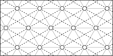
Figure 1: The schematic representation of Hamiltonian (2) on the triangular lattice [19]. The NN couplings are denoted by straight lines, whereas the anisotropic NNN couplings in two of the three directions are denoted by dotted lines.

The correlation function with the distance $r$ for the $q$-state Potts model including the Ising model ($q=2$) is given by

$$g_{i}(r)=\frac{q\delta_{s_{i}s_{i+r}}-1}{q-1}.$$ (3)

It assumes a value of $+1$ or $-1/(q-1)$.

We use three approaches to study the BKT transitions. The first approach is the machine-learning study which was developed by Shiina et al. [31], to classify the ordered, the BKT, and the disordered phases. A fully connected neural network is implemented with a standard library of TensorFlow of the 100-hidden unit model. For the spin data, we use the long-range correlation configuration with the distance of $L/2$ instead of the spin configuration itself. The average of the correlation along the $x$-axis and the $y$-axis is considered. For the training data, we use the results of the F six-state clock model [31]. For the test data, we investigate the correlation configurations of the AF three-state Potts model with F NNN coupling and that of the triangular AF Ising model with anisotropic NNN coupling. We classify the phases of these two models using the training data of the six-state clock model.

As the second approach, we perform the MC simulation of the ratio of the correlation functions of different distances, $R(T)=\langle g(L/2)\rangle/\langle g(L/4)\rangle$; for the two distances, we chose $L/2$ and $L/4$. Surungan et al. [28] made MC studies of the BKT transitions by investigating the correlation ratio and the size-dependent second-moment correlation length. Although there are other candidate quantities, we take the correlation ratio here. The correlation ratio has a single scaling variable for FSS

$$R(T)=\frac{\langle g(L/2)\rangle}{\langle g(L/4)\rangle}=\tilde{f}(L/\xi),$$ (4)

as in the Binder ratio [23], which is essentially the ratio of different moments. Here, $\xi$ stands for the correlation length. At the critical region, where the correlation length $\xi$ is infinite, the correlation ratio does not depend on the system size $L$. Thus, we expect the data collapsing of different sizes in the BKT phase. Above the upper BKT temperature $T_{2}$ and below the lower BKT temperature $T_{1}$, the data of different sizes start to separate. In the case of the BKT transition, the correlation length diverges as

$$\xi\propto\exp(c/\sqrt{|t|}),$$ (5)

where $t=T-T_{1,2}$. We employed the Metropolis local-update algorithm for the two models in combination with the replica-exchange algorithm [46] that overcomes slow dynamics. For the clock model we used the Swendsen-Wang cluster-update algorithm [47] in combination with the replica-exchange algorithm. The typical number of Monte Carlo steps was 200000 after discarding the first 10000 steps. Since the temperature exchange was typically performed for 40 temperatures, the effective Monte Carlo step number is much larger.

The third approach is the LS method employed in the previous publications [18, 19]. To make the explanations concrete, we shall borrow some notations there. Based on a dual sine-Gordon model, an effective field theory of the lattice models (see (2) in [18] and (4) in [19]), we analyzed the scaling dimensions of some local operators. For the upper BKT transition, the so-called ${\cal M}$ operator (a part of the Gaussian term) hybridizes with an operator $\sqrt{2}\cos\!\sqrt{2}\theta$ given in the disorder field and yields the ${\cal M}$-like operator with the dimension ${\bar{x}}_{0}$ [16]. We also focused on an operator $\sqrt{2}\sin 3\sqrt{2}\phi$ given in the order field with the dimension $x_{2}$. The numerical analysis of the eigenvalues of transfer matrices supposes a lattice model with a $L\times\infty$ cylindrical geometry. As explained in Refs. [18, 19], we can evaluate the renormalized scaling dimensions ${\bar{x}}_{0}(l)$ and $x_{2}(l)$ ($l=\ln L$) using discrete symmetry properties of these operators. We then obtained finite-size estimates of $T_{2}$ by the level-crossing condition

$${\bar{x}}_{0}(l)=\frac{16}{9}x_{2}(l).$$ (6)

For the lower BKT transition, the ${\cal M}$ operator hybridizes with $\sqrt{2}\cos 6\sqrt{2}\phi$ and yields another ${\cal M}$-like operator with $x_{0}$ [16]. We thus calculated finite-size estimates of $T_{1}$ by the level-crossing condition

$$x_{0}(l)=4x_{2}(l).$$ (7)

We compare the estimated BKT temperatures $T_{1,2}$ by three approaches.

3 AF three-state Potts model with ferromagnetic NNN coupling

Machine-learning study

We first show the results of the AF three-state Potts model with F NNN coupling. As a machine-learning study, the output layer averaged over a test set as a function of $T$ is plotted in figure 2. The data for $r$ = 0.2, 0.4, and 0.8 are given in (a), (b), and (c), respectively. The system sizes are 32, 48, and 64. For the training data, we use the F six-state clock model. We show the result of the previous study [31] for the F six-state clock model in figure 3, for convenience. The probabilities of predicting the phases are plotted at each temperature. The samples of $T$ within the ranges $0.4\leq T\leq 0.64$, $0.78\leq T\leq 0.82$ and $0.96\leq T\leq 1.2$ are used for the low-temperature, middle-temperature, and high-temperature training data, respectively. For a whole temperature range, around 35000 training data sets are used, and we use 500 test data sets for each temperature.

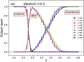
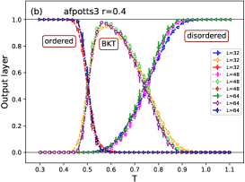
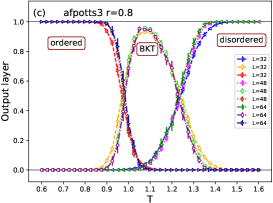
Figure 2: The output layer for the AF three-state Potts model with F NNN coupling for $r=0.2$ (a), $r=0.4$ (b), and $r=0.8$ (c), using the training data of the F six-state clock model. The system sizes are $L=32$, 48, and 64.

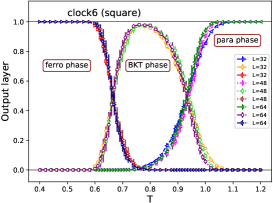
Figure 3: The output layer averaged over a test set as a function of $T$ for the 2D six-state clock model on the square lattice. The system sizes are $L$ = 32, 48, and 64. The samples of $T$ within the ranges $0.4\leq T\leq 0.64$, $0.78\leq T\leq 0.82$ and $0.96\leq T\leq 1.2$ are used for training data.

Figure 2 clearly shows the existence of three phases, the ordered phase, the intermediate phase, and the disordered phase. We estimate the size-dependent $T_{1,2}(L)$ from the point that the probabilities of predicting two phases are 50%. Systematic size dependence is not observed. The rough estimates of the transition temperatures, $T_{1}$ and $T_{2}$, are tabulated in table 1. We emphasize that the BKT transitions of a complex model, AF three-state Potts model on the square lattice with F NNN coupling can be studied by the training data of the six-state clock model.

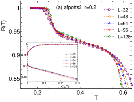
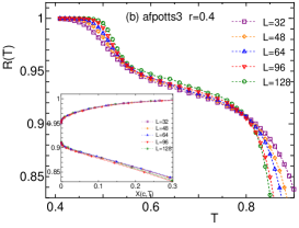
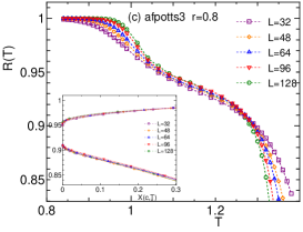
Figure 4: The plot of the correlation ratio $R(T)$ for the AF three-state Potts model on the square lattice with F NNN coupling. In the inset, the FSS plots are given, where $X(c,T)=L/\exp(c_{1,2}/\sqrt{|T-T_{1,2}|})$.

Monte Carlo study

We here show the MC results of the AF three-state Potts model on the square lattice with F NNN coupling. Following the study by Surungan et al. [28], we calculate the correlation ratio, $R(T)=\langle g(L/2)\rangle/\langle g(L/4)\rangle$, to investigate the BKT transitions. The results for $r$ = 0.2, 0.4, and 0.8 are plotted in figure 4. The system sizes are $L=32$, 48, 64, 96, and 128. We observe the collapsing curves of different sizes at intermediate temperature regimes and the spray out at lower and higher temperatures, which indicates the existence of two BKT transitions. The behavior of the collapsing is not good enough, compared to the regular six-state clock model [28], which may be attributed to the large corrections to FSS.

In the case of the BKT transition, the correlation length diverges as

$$\xi\propto\exp(c/\sqrt{|t|}),$$ (8)

where $t=T-T_{1,2}$. Thus, we can get the FSS plot if the temperature $T$ is scaled as $L/\exp(c_{1,2}/\sqrt{|T-T_{1,2}|})$, where $c$ is a fitting parameter. The FSS plots are given in the inset of figure 4.

The rough estimates of $T_{1}$ and $T_{2}$ are also tabulated in table 1.

Level-spectroscopy study

This model was studied using the LS method [18]. The phase diagram, in the space of $u=e^{-K_{1}}=e^{-J_{1}/T}$ and $v=e^{K_{2}}=e^{rJ_{1}/T}$, was given in figure 2 of [18]. The phase diagram is reproduced in figure 5, and the curves $v=e^{-r\ln(u)}$ with $r=0.2$, 0.4, and 0.8 are added. From the crossing point with these curves, we can read off the estimates of $T_{1}$ and $T_{2}$. The estimates are tabulated in table 1.

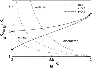
Figure 5: The phase diagram of the AF three-state Potts model on the square lattice with F NNN coupling using the LS method [18] in the space of $(u,v)$ = $(e^{-K_{1}},e^{K_{2}})$. The curves $v=e^{-r\ln(u)}$ with $r=0.2$, 0.4, and 0.8 are also plotted. From the crossing point with these curves, we can obtain the estimates of $T_{1}$ and $T_{2}$.

Table 1: The estimates of $T_{1}$ and $T_{2}$ for the AF three-state Potts model on the square lattice with F NNN coupling. The estimates of the LS method are based on the calculation in [18].

	$r=0.2$		$r=0.4$		$r=0.8$
	$T_{1}$	$T_{2}$	$T_{1}$	$T_{2}$	$T_{1}$	$T_{2}$
machine-learning	0.25	0.44	0.50	0.74	0.98	1.23
Monte Carlo	0.30	0.51	0.57	0.775	1.075	1.255
level-spectroscopy	0.277	0.490	0.554	0.755	1.056	1.240

By comparing various estimates of $T_{1}$ and $T_{2}$ tabulated in table 1, we see the consistency of various methods. The machine-learning study using the training data of the six-state clock model yields reasonable estimates.

4 Triangular AF Ising model with anisotropic NNN coupling

Machine-learning study

Next, we consider the triangular AF Ising model with anisotropic NNN coupling. Because the $q$-state clock models (XY model in the limit of $q\to\infty$) on the triangular lattice were not studied previously in the literature, the detailed calculation of the clock models on the triangular lattice is given in the Appendix.

As the result of the machine-learning study, we show the output layer averaged over a test set as a function of $T$ for the triangular AF Ising model with anisotropic NNN coupling in figure 6. For the training data, we use the F six-state clock model on the triangular lattice, which will be shown in the Appendix. The data for $r=0.2$, 0.4, and 0.8 are given in (a), (b), and (c), respectively. The system sizes are 24, 36, and 48. The probabilities of predicting the phases are plotted at each temperature. Figure 6 clearly demonstrates the existence of three phases, the ordered phase, the intermediate BKT phase, and the disordered phase. The rough estimates of the transition temperatures, $T_{1}$ and $T_{2}$, are tabulated in table 2.

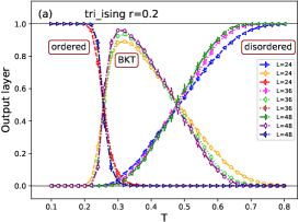
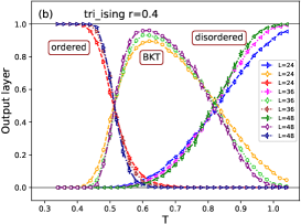
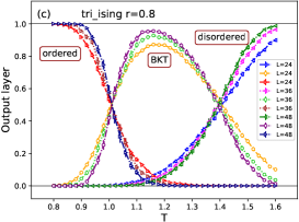
Figure 6: The output layer for the triangular AF Ising model with anisotropic NNN coupling for $r=0.2$ (a), $r=0.4$ (b), and $r=0.8$ (c), using the training data of the F six-state clock model. The system sizes are $L$ = 24, 36, and 48.

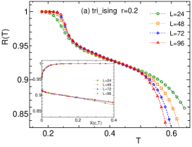
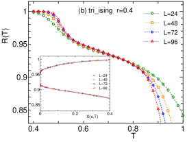
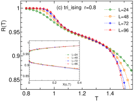
Figure 7: The plot of the correlation ratio $R(T)$ for the triangular AF Ising model with anisotropic NNN coupling. In the inset, the FSS plots are given, where $X(c,T)=L/\exp(c_{1,2}/\sqrt{|T-T_{1,2}|})$.

Monte Carlo study

We show the MC results of the correlation ratio, $R(T)$, of the triangular AF Ising model with anisotropic NNN coupling. The results for $r=0.2$, 0.4, and 0.8 are plotted in figure 7. The system sizes are $L=24$, 48, 72, and 96. We again observe the collapsing curves of different sizes at intermediate temperature regimes and the spray out at lower and higher temperatures. The behavior of the collapsing in the BKT phase is better than the case of the AF three-state Potts model on the square lattice with F NNN coupling (figure 4).

The FSS plots based on the exponential divergence of the correlation length are given in the inset of figure 7, where $T$ is scaled as $L/\exp(c_{1,2}/\sqrt{|T-T_{1,2}|})$.

The rough estimates of $T_{1}$ and $T_{2}$ are also tabulated in table 2.

Level-spectroscopy study

Otsuka et al. [19] studied this model using the LS method. The phase diagram, in the space of $u=e^{-K_{1}}=e^{-J_{1}/T}$ and $v=e^{K_{2}}=e^{rJ_{1}/T}$, is reproduced in figure 8, where the curves $v=e^{-r\ln(u)}$ with $r=0.2$, 0.4, and 0.8 are added. From the crossing point with the curve $v=e^{-r\ln(u)}$, we can obtain the estimates of $T_{1}$ and $T_{2}$. The estimates are tabulated in table 2.

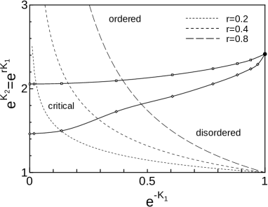
Figure 8: The phase diagram of the triangular AF Ising model with anisotropic NNN coupling using the level-spectroscopy method [19] in the space of $(u,v)$ = $(e^{-K_{1}},e^{K_{2}})$. The curves $v=e^{-r\ln(u)}$ with $r$ = 0.2, 0.4, and 0.8 are also plotted. From the crossing point with these curves, we can obtain the estimates of $T_{1}$ and $T_{2}$.

Table 2: The estimates of $T_{1}$ and $T_{2}$ for the triangular AF Ising model with anisotropic NNN coupling. The estimates of the level-spectroscopy method are based on the calculation in [19].

	$r=0.2$		$r=0.4$		$r=0.8$
	$T_{1}$	$T_{2}$	$T_{1}$	$T_{2}$	$T_{1}$	$T_{2}$
machine-learning	0.25	0.48	0.51	0.82	1.01	1.39
Monte Carlo	0.29	0.465	0.57	0.795	1.08	1.36
level-spectroscopy	0.271	0.494	0.547	0.801	1.070	1.330

We see the consistency of the estimates of $T_{1}$ and $T_{2}$ by various methods tabulated in table 2. We may say that the machine-learning study of this model yields reasonable estimates.

5 Effective exponents

In this section, we make a comment on the calculation of the decay exponent $\eta$ in the MC study, and discuss the self-dual point.

The correlation function with the distance $r$ decays as $g(r)\sim r^{-\eta(T)}$ at the critical point (line). We consider the correlation function with the distance $L/2$ for the finite system of the size $L$

$$g_{2}(L)=\langle\bm{s}(i)\cdot\bm{s}(i+L/2)\rangle.$$ (9)

We also consider

$$g_{4}(L)=\langle{\bm{s}}(i)\cdot{\bm{s}}(i+L/4)\rangle.$$ (10)

At the critical point (line), $g_{2}(L)$ behaves as $L^{-\eta(T)}$ and for $T<T_{1}$ and $T>T_{2}$, we may have the following relation:

$$g_{2}(L)\sim L^{-\eta(T)}f(L/\xi).$$ (11)

We examine the ratio of $g_{2}$ of the two sizes $L$ and $2L$:

$$\frac{g_{2}(L)}{g_{2}(2L)}=\frac{L^{-\eta}f(L/\xi)}{(2L)^{-\eta}f(2L/\xi)}=2^{-\eta}\frac{f(L/\xi)}{f(2L/\xi)}.$$ (12)

Then, we define the effective exponent $\eta_{\rm eff}$ by

$$\eta_{\rm eff}=\frac{\ln(g_{2}(L)/g_{2}(2L))}{\ln(2)}.$$ (13)

Theoretically, the critical exponent $\eta$ becomes 1/4 at $T_{2}$ and $4/q^{2}$ at $T_{1}$. We may estimate $T_{2}$ and $T_{1}$ from the condition that $\eta_{\rm eff}$ takes the theoretical value. The exponent $\eta_{\rm eff}$ is expected to take the temperature-dependent value for $T_{1}\leq T\leq T_{2}$; it does not depend on $L$, and there is no difference between $g_{2}$ and $g_{4}$. For $T<T_{1}$ and $T>T_{2}$, it becomes $L$-dependent, and $g_{2}$ and $g_{4}$ take different values. We show the calculated results of $\eta_{\rm eff}$ using (13) for the AF three-state Potts model with ferromagnetic NNN coupling in figure 9 and for the AF Ising model with anisotropic NNN coupling on the triangular lattice in figure 10, respectively. There, the theoretical values of $\eta_{2}=1/4$ and $\eta_{1}=1/9$ are shown by the dashed and dotted lines, respectively. Not only the data for $g_{2}$ but those for $g_{4}$ are given. We see an expected behavior of the temperature dependence of the effective exponent $\eta_{\rm eff}$ in figures 9 and 10. The temperatures at which $\eta_{1,2}$ take the theoretical values are consistent with the estimates of $T_{1}$ and $T_{2}$ in tables 1 and 2.

In the Villain model, where the exact duality transformation holds, the exponent $\eta$ becomes $1/q$ at the self-dual (sd) point. Moreover, there is an exact relation between the temperatures:

$$T_{1}T_{2}=4\pi^{2}/q^{2},\quad{\rm therefore},\quad T_{\rm sd}=2\pi/q.$$ (14)

Although this self-dual point is particular to the Villain model, we give the value of $\eta_{\rm eff}$, $1/q$, in figures 9 and 10, by the dash-dotted lines. Let us denote the temperature $T_{\rm sd}$ by the condition that $\eta_{\rm eff}$ takes the self-dual value $\eta_{\rm sd}$. We can see that $T_{\rm sd}$ is close to the temperature at which the probability of predicting the BKT phase takes the maximum in Figs. 2 and 6 in the machine-learning studies. We note that for the triangular AF Ising model with anisotropic NNN coupling, the self-dual temperature was discussed using the LS method [19].

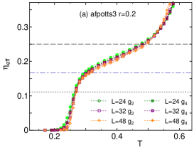
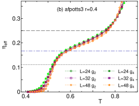
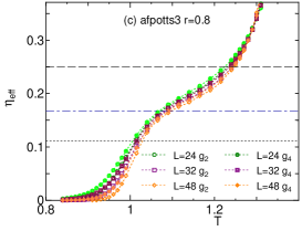
Figure 9: The effective exponents $\eta_{\rm eff}$, calculated by (13), for AF three-state Potts model with F NNN coupling (square lattice). The theoretical values of $\eta_{2}=1/4$, $\eta_{\rm sd}=1/6$, and $\eta_{1}=1/9$, are shown by the dashed, dash-dotted, and dotted lines, respectively.

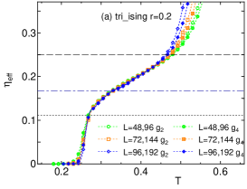
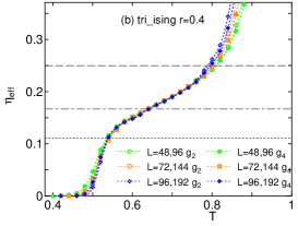
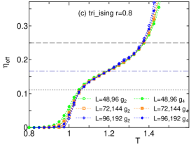
Figure 10: The effective exponents $\eta_{\rm eff}$, calculated by (13), for the AF Ising model with anisotropic NNN coupling (triangular lattice). The theoretical values of $\eta_{2}=1/4$, $\eta_{\rm sd}=1/6$, and $\eta_{1}=1/9$ are shown by the dashed, dash-dotted, and dotted lines, respectively.

6 Summary and discussion

We used the machine-learning study for the AF three-state Potts model on the square lattice with F NNN coupling and the triangular AF Ising model with anisotropic NNN coupling. We classified the ordered, the BKT, and the disordered states using the training data of the F six-state clock model. We explicitly showed the universal behavior of implicit symmetries in totally different models.

We also used the MC studies paying attention to the correlation ratio, which is appropriate in studying the BKT transitions. In the recent publication on the antiferromagnetic Potts model [48], the authors pointed out that the Binder ratio is not necessarily the best method in determining the critical point as in Refs. [27] and [24]. The two BKT transitions were determined with precision using the valid metric of correlation ratios, confirming the six-state clock universality.

Comparing the results of the machine-learning study and the MC simulation with the previous results of the LS method [18, 19], we confirmed the six-state clock universality for the AF three-state Potts model on the square lattice with F NNN coupling and the triangular AF Ising model with anisotropic NNN coupling.

We make a brief comment on a future study. Surface effects are important subjects of critical phenomena, and the extraordinary-log phase has captured recent attention. With this regard, recently the three-dimensional six-state clock model [49] and the three-dimensional three-state antiferromagnetic Potts model [48] with a free surface were studied. The application of the present approaches to these models will be interesting problems.

Universality is an essential concept in phase transitions. We performed a comprehensive study on the six-state clock universality in completely different models. In future research, we would like to explore the six-state clock universality in other models.

Appendix. $\bm{XY}$ and six-state clock models on the triangular lattice

The reports on the XY or clock models on the triangular lattice have not been found in the literature. Only the exception is the MC study of the XY model by Sorokin [50]. By using the MC study of the helicity modulus, the BKT temperature was estimated as 1.418(2). We here show our MC results on the XY model and the six-state clock model on the triangular lattice. We also perform a machine-learning study.

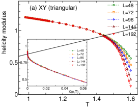
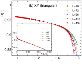
Figure 11: Helicity modulus (a) and correlation ratio (b) for XY model on the triangular lattice. The system sizes are 48, 72, 96, 144, and 192. In the plot of helicity modulus, we give the straight line $(2/\pi)T$. In the inset the FSS plots are given, where $X(c,T)=L/\exp(c_{2}/\sqrt{|T-T_{2}|})$.

The MC results on the XY model and the six-state clock model are plotted in Figs. 11 and 12, respectively. The helicity modulus and correlation ratio $R(T)$ are plotted in both figures. The system sizes are 48, 72, 96, 144, and 192. In the plot of helicity modulus, we give the straight line $(2/\pi)T$. The crossing point gives a universal jump. The $q$-state clock model, a discrete version of the XY model, experiences two BKT transitions because of the discreteness. We note that there is no anomaly in helicity modulus for the lower transition, $T_{1}$. The BKT phase is indicated by the collapsing curves of different sizes in the plot of $R(T)$. It is a direct consequence of the power law behavior of the correlation function at the BKT phase. The spray out of the curves at lower and higher temperatures signifies BKT transitions. The rough estimates of the BKT temperatures are $T_{2}$ = 1.43 for the XY model, and $T_{2}$=1.44 and $T_{1}$ = 1.12 for the six-state clock model. The result of the XY model is consistent with the report by Sorokin [50]. The values of the triangular lattice are roughly 3/2 of those of the square lattice. It is because the coordination number of the triangular lattice is six, whereas that of the square lattice is four.

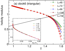
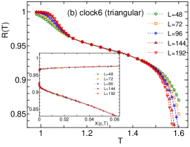
Figure 12: Helicity modulus (a) and correlation ratio (b) for the six-state clock model on the triangular lattice. The system sizes are 48, 72, 96, 144, and 192. In the plot of helicity modulus, we give the straight line $(2/\pi)T$. In the inset the FSS plots are given, where $X(c,T)=L/\exp(c_{1,2}/\sqrt{|T-T_{1,2}|})$. For the helicity modulus, only the FSS for the high-temperature side is given.

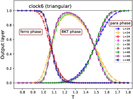
Figure 13: The output layer averaged over a test set as a function of $T$ for the triangular lattice six-state clock model. The system sizes are $L=24$, 36, and 48. The samples of $T$ within the ranges $0.76\leq T\leq 1.04$, $1.21\leq T\leq 1.31$ and $1.52\leq T\leq 1.8$ are used for training data.

We also show the results of the machine-learning study. The output layer averaged over a test set as a function of $T$ for the triangular F six-state model is shown in figure 13. The system sizes are 24, 36, and 48. The samples of $T$ within the ranges $0.76\leq T\leq 1.04$, $1.21\leq T\leq 1.31$ and $1.52\leq T\leq 1.8$ are used for the low-temperature, middle-temperature, and high-temperature training data, respectively. The probabilities of predicting the phases are plotted at each temperature. We clearly observe three phases, the ordered, the BKT, and the disordered phases. We estimate the size-dependent $T_{1,2}(L)$ from the point that the probabilities of predicting two phases are 50%. Systematic size dependence is not observed. The rough estimates of $T_{1}$ and $T_{2}$ are 1.07 and 1.48, respectively. The estimates are compatible to those of the MC study. However, the BKT phase is slightly wider, which is the same situation as the case of the square lattice. It comes from the finite-size effects.

References

- [1]
- [2] L. P. Kadanoff, W. Götze, D. Hamblen, R. Hecht, E. A. S. Lewis, V. V. Palciauskas, M. Rayl, J. Swift, D. Aspnes, and J. Kane 1967 Static Phenomena Near Critical Points: Theory and Experiment Rev. Mod. Phys. 39 395.
- [3] L. P. Kadanoff 1990 Scaling and universality in statistical physics Physica A 163 1.
- [4] V. L. Berezinskii 1970 Destruction of Long-range Order in One-dimensional and Two-dimensional Systems having a Continuous Symmetry Group I. Classical Systems Sov. Phys. JETP 32 493.
- [5] V. L. Berezinskii 1972 Destruction of Long-range Order in One-dimensional and Two-dimensional Systems Possessing a Continuous Symmetry Group. II. Quantum Systems Sov. Phys. JETP 34 610.
- [6] J. M. Kosterlitz and D. Thouless 1973 Ordering, metastability and phase transitions in two-dimensional systems J. Phys. C: Solid State Phys. 6 1181.
- [7] J. M. Kosterlitz 1974 The critical properties of the two-dimensional xy model J. Phys. C: Solid State Phys. 7 1046.
- [8] J. V. José, L. P. Kadanoff, S. Kirkpatrick, and D. R. Nelson 1977 Renormalization, vortices, and symmetry-breaking perturbations in the two-dimensional planar model Phys. Rev. B 16 1217.
- [9] S. Elitzur, R. B. Pearson, and J. Shigemitsu 1979 Phase structure of discrete Abelian spin and gauge systems Phys. Rev. D 19 3698.
- [10] J. Villain 1975 Theory of one- and two-dimensional magnets with an easy magnetization plane. II. The planar, classical, two-dimensional magnet J. Phys. (Paris) 36 581.
- [11] J.-P. Lv, Y. Deng, J. L. Jacobsen, and J. Salas 2018 The three-state Potts antiferromagnet on plane quadrangulations J. Phys. A: Math. Theor. 51 365001.
- [12] M. P. M. den Nijs, M. P. Nightingale, and M. Schick 1982 Critical fan in the antiferromagnetic three-state Potts model Phys. Rev. B 26 2490.
- [13] J. L. Cardy 1981 Antiferromagnetic clock models in two dimensions Phys. Rev. B 24 5128.
- [14] H. Kitatani and T. Oguchi 1988 Antiferromagnetic Triangular Ising Model with Ferromagnetic Next Nearest Neighbor Interactions-Transfer Matrix Method- J. Phys. Soc. Jpn. 57 1344.
- [15] K. Nomura and K. Okamoto 1994 Critical properties of antiferromagnetic XXZ chain with next-nearest-neighbour interactions J. Phys. A: Math, Gen. 27 5773.
- [16] K. Nomura 1995 Correlation functions of the 2D sine-Gordon model J. Phys. A: Math, Gen. 28 5451.
- [17] M. Nakamura, K. Nomura, and, A. Kitazawa 1997 Renormalization Group Analysis of the Spin-Gap Phase in the One-Dimensional - Model Phys. Rev. Lett. 79 3214.
- [18] H. Otsuka, K. Mori, Y. Okabe, and K. Nomura 2005 Level spectroscopy of the square-lattice three-state Potts model with a ferromagnetic next-nearest-neighbor coupling Phys. Rev. E 72 046103.
- [19] H. Otsuka, Y. Okabe, and K. Nomura 2006 Global phase diagram and six-state clock universality behavior in the triangular antiferromagnetic Ising model with anisotropic next-nearest-neighbor coupling: Level-spectroscopy approach Phys. Rev. E 74 011104.
- [20] D. P. Landau and K. Binder 2014 A guide to MC Simulations in Statistical Physics (Cambridge: Cambridge University Press).
- [21] M. N. Barber 1983 in Phase Transitions and Critical Phenomena, vol. 8 ed C. Domb and J. Lebowitz (New York: Academic Press).
- [22] J. L. Cardy 1988 Finite Size Scaling ed J. L. Cardy (Amsterdam: North-Holland).
- [23] K. Binder 1981 Finite size scaling analysis of ising model block distribution functions Z. Phys. B 43 119.
- [24] M. Hasenbusch 2008 The Binder cumulant at the Kosterlitz-Thouless transition J. Stat. Mech. P08003.
- [25] W. Janke 1997 Logarithmic corrections in the two-dimensional XY model Phys. Rev. B 55 3580.
- [26] Y. Tomita and Y. Okabe 2002 Finite-size scaling of correlation ratio and generalized scheme for the probability-changing cluster algorithm Phys. Rev. B 66 180401(R).
- [27] H. G. Katzgraber, M. Körner, and A. P. Young 2006 Universality in three-dimensional Ising spin glasses: A Monte Carlo study Phys. Rev. B 73 224432.
- [28] T. Surungan, S. Masuda, Y. Komura, and Y. Okabe 2019 Berezinskii-Kosterlitz-Thouless transition on regular and Villain types of -state clock models J. Phys. A: Math. Theor. 52 275002.
- [29] G. Carleo, I. Cirac, K. Cranmer, L. Daudet, M. Schuld, N. Tishby, L. Vogt-Maranto, and L. Zdeborová 2019 Rev. Mod. Phys. 91 045002.
- [30] J. Carrasquilla and R. G. Melko 2017 Machine learning phases of matter Nat. Phys. 13 431.
- [31] K. Shiina, H. Mori, Y. Okabe, and H. K. Lee 2020 Machine-Learning Studies on Spin Models Sci. Rep. 10 2177.
- [32] Y. Tomita, K. Shiina, Y. Okabe, and H. K. Lee 2020 Machine-learning study using improved correlation configuration and application to quantum Monte Carlo simulation Phys. Rev. E 102 021302(R).
- [33] P. W. Kasteleyn and C. M. Fortuin 1969 Phase Transitions in Lattice Systems with Random Local Properties J. Phys. Soc. Jpn. Suppl. 26 11.
- [34] C. M. Fortuin and P. W. Kasteleyn 1972 On the random-cluster model: I. Introduction and relation to other models Physica 57 536.
- [35] U. Wolff 1990 Asymptotic freedom and mass generation in the O(3) nonlinear -model Nucl. Phys. B 334 581-610.
- [36] H. G. Evertz, G. Lana, and M. Marcu 1993 Cluster algorithm for vertex models Phys. Rev. Lett. 70 875.
- [37] Y. Miyajima, Y. Murata, Y. Tanaka, and M. Mochizuki 2021 Machine-learning detection of the Berezinskii-Kosterlitz-Thouless transitions in the -state clock models Phys. Rev. B 104 075114.
- [38] W. J. Hu, R. Singh, and R. Scalettar 2017 Discovering phases, phase transitions, and crossovers through unsupervised machine learning: A critical examination Phys. Rev. E 95 062122.
- [39] C. Wang and H. Zhai 2017 Machine learning of frustrated classical spin models. I. Principal component analysis Phys. Rev. E 96 144432.
- [40] K. Shiina, H. Mori, Y. Tomita, H. K. Lee, and Y. Okabe 2021 Inverse renormalization group based on image super-resolution using deep convolutional networks Sci. Rep. 11 9617.
- [41] Z.-Q. Li, L.-P. Yang, Z. Y. Xie, H.-H. Tu, H.-J. Liao, and T. Xiang 2020 Critical properties of the two-dimensional -state clock model Phys. Rev. E 101 060105(R).
- [42] S. Hong and D.-H. Kim 2020 Logarithmic finite-size scaling correction to the leading Fisher zeros in the -state clock model: A higher-order tensor renormalization group study Phys. Rev. E 101 012124.
- [43] H. Ueda, K. Okunishi, K. Harada, R. Krčmár, A. Gendiar, S. Yunoki, and T. Nishino 2020 Finite- scaling analysis of Berezinskii-Kosterlitz-Thouless phase transitions and entanglement spectrum for the six-state clock model Phys. Rev. E 101 062111.
- [44] G. Li, K. H. Pai, and Z.-C. Gu 2022 Tensor-network renormalization approach to the -state clock model Phys. Rev. Research 4 023159.
- [45] H. Chen, P. Hou, S. Fang, and Y. Deng 2022 Monte Carlo study of duality and the Berezinskii-Kosterlitz-Thouless phase transitions of the two-dimensional -state clock model in flow representations Phys. Rev. E 106 024106.
- [46] K. Hukushima and K. Nemoto 1996 Exchange Monte Carlo Method and Application to Spin Glass Simulations J. Phys. Soc. Jpn. 65 1604.
- [47] R. H. Swendsen and J. S. Wang 1987 Nonuniversal critical dynamics in Monte Carlo simulations Phys. Rev. Lett. 58 86.
- [48] L.-R. Zhang, C. Ding, Y. Deng, and L. Zhang 2022 Surface criticality of the antiferromagnetic Potts model Phys. Rev. B 105 224415.
- [49] X. Zou, S. Liu, and W. Guo 2022 Surface critical properties of the three-dimensional clock model Phys. Rev. B 106 064420.
- [50] A. O. Sorokin 2019 Critical density of topological defects upon a continuous phase transition Ann. Phys. (Amsterdam) 411 167952.