GTree: GPU-Friendly Privacy-preserving Decision Tree Training and Inference

Abstract

Decision tree (DT) is a widely used machine learning model due to its versatility, speed, and interpretability. However, for privacy-sensitive applications, outsourcing DT training and inference to cloud platforms raise concerns about data privacy. Researchers have developed privacy-preserving approaches for DT training and inference using cryptographic primitives, such as Secure Multi-Party Computation (MPC). While these approaches have shown progress, they still suffer from heavy computation and communication overheads. Few recent works employ Graphical Processing Units (GPU) to improve the performance of MPC-protected deep learning. This raises a natural question: can MPC-protected DT training and inference be accelerated by GPU?

We present GTree, the first scheme that uses GPU to accelerate MPC-protected secure DT training and inference. GTree is built across 3 parties who securely and jointly perform each step of DT training and inference with GPU. Each MPC protocol in GTree is designed in a GPU-friendly version. The performance evaluation shows that GTree achieves ${\thicksim}11{\times}$ and ${\thicksim}21{\times}$ improvements in training SPECT and Adult datasets, compared to the prior most efficient CPU-based work. For inference, GTree shows its superior efficiency when the DT has less than 10 levels, which is $126\times$ faster than the prior most efficient work when inferring $10^{4}$ instances with a tree of 7 levels. GTree also achieves a stronger security guarantee than prior solutions, which only leaks the tree depth and size of data samples while prior solutions also leak the tree structure. With oblivious array access, the access pattern on GPU is also protected.

I Introduction

The decision tree (DT) is a powerful and versatile Machine learning (ML) model that can be applied to a wide range of use cases across various domains. Its ability to handle both categorical and numerical data, noisy data, and high-dimensional data, and its interpretability make it a popular choice for many applications, such as fraud detection, medical diagnosis, and weather prediction. To train a DT model and make predictions efficiently, an efficient solution is to outsource the tasks to cloud platforms, but with privacy costs as the underlying data could be highly sensitive. For privacy-sensitive applications, such as health care, all the data samples, the trained model, the inference results and any intermediate data generated during the model training and inference should be carefully protected from the Cloud Service Provider (CSP). This has led to the development of privacy-preserving approaches for DT training and inference.

The typical way to achieve a privacy-preserving DT system is to employ traditional cryptographic primitives, such as Secure Multi-Party Computation (MPC/SMC) [1, 2, 16, 21, 26, 28, 41, 47, 56] and Homomorphic Encryption (HE) [7, 54, 44, 3], or a combination of both [48, 28]. MPC enables the data provider and the ML service provider to perform the training and/or inference jointly without revealing any party’s private inputs, and HE allows the ML service provider to perform certain computations over ciphertext. Nevertheless, the majority of the existing approaches are still not secure enough. Earlier works, such as [16, 26], focus mainly on the input data privacy while do not consider the model. Many works, such as [21, 28, 41], leak statistical information and tree structures from which the adversary could infer other sensitive information [2, 10]. Existing approaches also suffer from heavy computation and communication overheads. For instance, the most recent privacy-preserving DT approach proposed in [28] takes over 20 minutes and ${\thicksim}2$ GB communication cost to train a tree of depth 7 with 958 samples and 9 categorical features.

Many recent works [35, 25, 52] show that Trusted Execution Environment (TEE) is a more efficient tool to design privacy-preserving DT systems. With TEE’s protection, the data can be processed in plaintext. However, TEEs such as Intel SGX [12] have limited computational power compared with Graphic Processing Units (GPUs). Processing all the DT tasks inside the TEE still cannot achieve ideal performance. GPU TEEs such as Graviton [49] require hardware modification which would adversely affect compatibility.

Hardware acceleration with GPUs is playing a critical role in the evolution of modern ML. Several recent works [31, 34, 45, 53] have utilized GPU to accelerate privacy-preserving deep learning. Secure neural network training can easily leverage the benefits of the GPU due to massive GPU-friendly operations (e.g., convolutions and matrix multiplications). Such investigation raises the natural question: can secure DT training and inference benefit from GPU acceleration?

Our Goals and Challenges. In this work, we aim to design a GPU-based system to securely train a DT model and make predictions. Specifically, our approach does not reveal any information other than the size of the input data (i.e., training and query data) and the depth of the tree.

GPUs are especially effective when dealing with grid-like data structures such as arrays and matrices [13]. In order to better utilize GPU acceleration, we represent the DT and data structures as arrays and perform both training and inference on the arrays in GTree. However, processing such a structure securely on GPU is non-trivial because it suffers from access pattern leakage, which enables an adversary to infer the shape of the tree. Thus, the first challenge is to protect the access patterns on GPU.

To protect the data and the DT, we employ MPC in both training and inference. However, inappropriate MPC protocols could impede GPU acceleration. The resources of GPU will be sufficiently utilized when performing a large number of simple arithmetic computations (e.g., addition and multiplication) on massive data in parallel. The operations involve a large number of conditional statements, modular reduction, and non-linear functions, e.g., exponentiation and division are less well-suited for GPU. For instance, recent work CryptGPU [45] shows that GPU achieves much less performance gain when evaluating non-linear functions in the context of private training over a neural network. Thus, the second challenge is to design GPU-friendly MPC protocols for DT training and inference so as to take full advantage of GPU parallelism.

Our contributions. In this work, we introduce GTree, a GPU-based privacy-preserving DT training and inference system addressing the above two challenges. To the best of our knowledge, GTree is the first scheme that deploys secure DT training and inference on the GPU. GTree relies on secret-sharing-based MPC protocol, which is more suitable to GPU than Yao’s garbled circuits (GC) [55]. Basically, GTree involves 3 non-colluding parties and securely shares the data and model via 2-out-of-3 replicated secret sharing [5]. Both the training and inference are performed jointly by the 3 parties. To protect access patterns, we design a GPU-based oblivious array access protocol, where the parties can jointly get the shares of the target element of an array with the secret-shared index without learning which element is actually accessed. To make GTree GPU-friendly, we encode the tree in a way that it can be always trained level by level in parallel, and we minimize conditional statements for all protocols. Furthermore, our protocols mainly involve simple arithmetic operations which are particularly suitable for GPU.

We implemented a prototype of GTree on top of the general-purpose GPU-based MPC platform Piranha [53], and evaluate its performance on a server equipped with 3 NVIDIA Tesla V100 GPUs. The results show that GTree takes about 0.31 and 4.32 seconds to train with SPECT and Adult datasets, respectively, which is ${\thicksim}11{\times}$ and ${\thicksim}21{\times}$ faster than the previous work [21] (GTree also provides a stronger security guarantee than it). We also compare GTree with an SGX-based solution, called SGX only which processes all tasks within an enclave. To train $5{\times}10^{4}$ data samples with 64 features, GTree outperforms SGX only by ${\thicksim}27{\times}$. As for DT inference, GTree shows its superior efficiency when the tree has less than 10 levels. GTree outperforms the prior most efficient solution [23] by  $126\times$ for inferring $10^{4}$ instances when the tree depth is 7. Compared with SGX-only, GTree is more efficient to infer a batch of instances when the tree depth is less than 6.

Overall, GTree achieves not only better performance but also a stronger security guarantee than previous CPU-based works. GTree protects the statistical information of data samples, the tree shape, and tree access patterns while most prior works can only protect the data samples and/or the model. Finally, we formally prove the security of GTree.

II Background

In this section, we present the basic information of DT and the cryptographic primitives used in GTree.

II-A Decision Tree

A decision tree consists of internal nodes and leaves, where each internal node is associated with a test on a feature, each branch represents the outcome of the test, and each leaf represents a label which is the decision taken after testing all the features on the corresponding path.

Training. The model is trained with labeled data samples and a data sample contains a set of feature values and a label. Building a DT is the process of converting each leaf into an internal node by assigning a feature to it and splitting new leaves until all leaves get labels. Which feature is the best option for a leaf is measured with a heuristic measurement, e.g., gini index or information gain [38], and such measurement requires statistical information of the data samples partitioned to the leaf. The process starts from a leaf (i.e., the root) and all data samples are assigned to it. Building a DT includes the following 3 steps:

1. Learning phase: when a leaf is converted into an internal node, partition its data samples into new leaves based on the assigned feature. For binary trees, each feature only has two values, say $v_{0}$ or $v_{1}$. The data samples with values $v_{0}$ and $v_{1}$ are assigned to the left and the right new leaves, respectively. After that, at each new leaf, for each possible $(value,label)$ pair, count the number of data samples containing it.

2. Heuristic computation: if all the data samples at a new leaf only contain a label value, the label value is assigned to the leaf; otherwise, compute the heuristic measurements (GTree uses gini index [37]) for each feature, then select the best feature to split the leaf. For a feature $s$ and dataset $\bm{D}$, the gini index is defined as follows:

   $$\footnotesize\begin{split}&\overline{G}(\bm{D})=1-\sum_{k=1}^{|V_{s_{d-1}}|}(\frac{|\bm{D}_{k}|}{|\bm{D}|})^{2}\\ &\overline{G}(\bm{D},s)={\sum}_{i=0}^{|V_{s}|-1}\frac{|\bm{D}^{v_{s,i}}|}{|\bm{D}|}\overline{G}(\bm{D}^{v_{s,i}})\end{split}$$ (1)

   where $|\bm{D}_{k}|$ is the number of samples containing $k$-th label and $k\in[1,|V_{s_{d-1}}|]$, $|V_{s}|$ is the number of values of feature $s$ (which is 2 for binary trees and $s_{d-1}$ indicates the label) and $\bm{D}^{v_{s,i}}$ represents a subset of $\bm{D}$ containing feature $s$ with value of $v_{s,i}$.

3. Node split: convert the leaf into an internal node using the best feature.

Inference To infer an unlabelled data sample (or data instance), from the root node, we check whether the corresponding feature value of the data instance is $v_{0}$ or $v_{1}$, and continue the test with its left or right child respectively, until a leaf node. The label value of the accessed leaf is the inference result.

II-B Secret Sharing

In GTree, the data and queries are secretly shared among three parties with 2-out-of-3 replicated secret sharing (RSS) [5]. We denote $P_{1},P_{2}$, and $P_{3}$ as the three parties. For clarity, we denote the previous and next party of $P_{i}$ as $P_{i-1}$ and $P_{i+1}$, respectively, where $i\in\{1,2,3\}$. Notably, $P_{3+1}$ is $P_{1}$ and $P_{1-1}$ is $P_{3}$. GTree leverages Arithmetic/Boolean sharing to share data. Given input $x$, we use $\langle x\rangle^{A}$ and $\langle x\rangle^{B}$ to denote its Arithmetic sharing and Boolean sharing, respectively.

Arithmetic Sharing. An $l$-bit value $x$ (integers modulo $2^{l}$) is additively shared in the ring $\mathbb{Z}_{2^{l}}$ as a sum of 3 values. Here we model it with the following operations:

• $\mathtt{Share}^{A}(x)\rightarrow(x_{1},x_{2},x_{3})$: On input $x\in\mathbb{Z}_{2^{l}}$, it samples $x_{1},x_{2},x_{3}{\in}\mathbb{Z}_{2^{l}}$ such that $x_{1}+x_{2}+x_{3}=x\mod 2^{l}$. $P_{i}$ holds $(x_{i},x_{i+1})$. We denote $\langle x\rangle^{A}=(x_{1},x_{2},x_{3})$.

• $\mathtt{Reconstruct}^{A}(\langle x\rangle^{A})\rightarrow x$: On input $\langle x\rangle^{A}=(x_{1},x_{2},x_{3})$, it outputs $x=x_{1}+x_{2}+x_{3}\mod 2^{l}$. $P_{i}$ receives $x_{i-1}$ from $P_{i-1}$ and then computes $x$ locally.

• Addition $\langle z\rangle^{A}=\langle x\rangle^{A}+\langle y\rangle^{A}$: $z_{i}=x_{i}+y_{i}\mod 2^{l}$. Note that $P_{i}$ can locally compute $(z_{i},z_{i+1})$ with $(x_{i},x_{i+1})$ and $(y_{i},y_{i+1})$.

• Linear operation: Given public constants ${\alpha},{\beta}~{}{\in}~{}\mathbb{Z}_{2^{l}}$, each party computes their respective shares of $\langle{\alpha}x+{\beta}\rangle^{A}=({\alpha}x_{1}+{\beta},{\alpha}x_{2},{\alpha}x_{3})$ locally.

• Multiplication $\langle z\rangle^{A}=\langle x\rangle^{A}\cdot\langle y\rangle^{A}$: $z_{i}=x_{i}*y_{i}+x_{i+1}*y_{i}+x_{i}*y_{i+1}$. With $(x_{i},x_{i+1})$ and $(y_{i},y_{i+1})$, $P_{i}$ can only compute $z_{i}$ locally, which is one additive secret sharing of $z$. To make sure all parties hold replicated shares of $z$, $P_{i}$ sends $P_{i+1}$ a blinded share $z_{i}+{\alpha}_{i}$, where ${\alpha}_{1},{\alpha}_{2},{\alpha}_{3}{\in}\mathbb{Z}_{2^{l}}$ and ${\alpha}_{1}+{\alpha}_{2}+{\alpha}_{3}=0$ [32].

The above operations can be generalized to vector operations. For instance, $\langle\bm{X}\rangle^{A}=(\langle a\rangle^{A},\langle b\rangle^{A},...)$, $\langle\bm{X}\rangle^{A}+\langle\bm{X^{\prime}}\rangle^{A}=(\langle a\rangle^{A}+\langle a^{\prime}\rangle^{A},\langle b\rangle^{A}+\langle b^{\prime}\rangle^{A},...)$.

Boolean Sharing. Boolean sharing uses an XOR-based secret sharing. For simplicity, given $l$-bit values, we assume each operation is performed $l$ times in parallel. The sharing semantics and the operations are the same as the arithmetic shares except that $+$ and $\cdot$ are respectively replaced by bit-wise $\oplus$ and $\wedge$.

III Overview of GTree

In this section, we describe the system model and design overview.

III-A System Model

GTree consists of 3 types of entities: the Data Owner (DO), the Query User (QU), and the Cloud Service Provider (CSP). GTree employs 3 independent CSPs, such as Facebook, Google, and Microsoft, and they should be equipped with GPUs. The DO outsources data samples to the three CSPs securely with RSS for training the DT, and the QU queries the system after the training period for data classification or prediction.

III-B Threat Model

As done in many other three-party-based systems [32, 45, 51], GTree resists a semi-honest adversary with an honest majority among the three parties. Specifically, two of the CSPs are fully honest, and the third one is semi-honest, i.e., follows the protocol but may try to learn sensitive information, e.g., tree structure, by observing and analyzing the access patterns and other leakages. The DO and QU are fully trusted. We assume the three parties maintain secure point-to-point communication channels and share pairwise AES keys to generate common randomness. We assume the private keys of the parties are stored securely and not susceptible to leakage. Note that as the QU receives the answers to the queries in the clear, GTree does not guarantee to protect the privacy of the training data from attacks such as model inversion and membership inference [43, 46]. Defending against these attacks is an orthogonal problem and is out of the scope of this work. Additionally, GTree does not protect against denial-of-service attacks [19] and other attacks based on physical information.

III-C Design Overview

GTree uses MPC to ensure the security of the whole system. ABY³ [32] and Piranha [53] show that, in most cases, RSS-based 3-Party Computation (3PC) is more efficient than 2- or $N$-PC ($N>3$) in terms of runtime and communication cost. Thus, our MPC framework involves 3 CSPs. Moreover, GTree adopts secret sharing to implement the 3PC protocol, which is GPU-friendly and more efficient than GC when computing low-level circuits. Specifically, the DO and QU protect data samples and queries with 2-out-of-3 RSS before sending them to the CSPs. The three CSPs use the shared data to train the model and predicate queries collaboratively.

GTree adopts 3 strategies to protect the tree structure: representing the tree and intermediate data into arrays, training the tree level by level, and always padding the tree into a complete binary tree with dummy nodes. As a result, adversaries can only learn the tree depth. Such design also enables GTree to parallelize the training and inference tasks as much as possible.

Either for training or inference, the access pattern over an array should be protected even when the array is encrypted; otherwise, adversaries could infer sensitive information. For instance, the similarity among data samples/instances can be inferred from the tree access patterns, and if some of them are known to an adversary, she/he can infer the others and further infer tree information. We design a GPU-friendly Oblivious Array Access protocol, and the main idea is to scan the array linearly, i.e., access every element of the array and use secret-sharing-based select function (i.e., $\mathtt{SelectShare}$ [51]) to ensure that only the desired element is actually read or written.

To make DT training and inference GPU-friendly, our main idea is to parallelize as many operations as possible. On the one hand, GTree always ensures the tree is complete and trains all the leaves at the same level concurrently based on a novel tree encoding method. On the other hand, all the protocols mainly involve simple arithmetic operations and contain minimized conditional statements so that they are highly parallelable.

IV Data and Model Representation

TABLE I: Notations

Notation	Description
$\bm{D}$	Data samples array where $|\bm{D}|=N_{D}$
$d$	Number of features
$\bm{S}$	A sequence of $d$ features, $\bm{S}=(s_{0},s_{1},{\cdots},s_{d-1})$
$\bm{V}_{s_{i}}$	Values of feature $s_{i}$, $\bm{V}_{s_{i}}=(v_{i,0},v_{i,1})$, i.e., binary feature
$n_{h}$	Number of nodes at level $h$, $n_{h}=2^{h}$
${\Psi}_{r_{i}}$	Number of data samples at a leaf containing the $i$-th label, where $i{\in}[0,1]$
$\overline{G}(\cdot)$	Heuristic measurement, i.e., Information Gain or Gini Index
$\bm{T}$	Tree array stores tree nodes (i.e., internal, leaf and dummy nodes). $\bm{T}[2i+1]$ and $\bm{T}[2i+2]$ are the left and right children of $\bm{T}[i]$, respectively
$\bm{F}$	Node type array indicates the node type of $\bm{T}[i]$ where $|\bm{F}|=|\bm{T}|$ and $\bm{F}[i]=0,1,2$ corresponds to internal, leaf and dummy node.
$\bm{M}$	An array indicating the leaf each data sample $\bm{D}[i]$ currently belongs to, where $|\bm{M}|=|\bm{D}|$
$c_{(value,label)}$	Frequency of each $(value,label)$
$\bm{C}$	2D-counter array has 3 rows and $2(d-1)$ columns, storing the frequency of each feature
$\bm{\gamma}$	An array indicating if each feature has been assigned to a leaf node or not, where $|\bm{\gamma}|=d-1$

This section presents how data and the decision tree are represented in GTree. In the rest of this paper, we will use the notation shown in Table I.

IV-A Data Representation

We stress that GTree focuses on training categorical features. We assume that $\bm{S}=(s_{0},s_{1},{\cdots},s_{d-1})$ represents a sequence of $d$ features, where each feature $s_{i}$ having two possible values (i.e., binary features): $\bm{V}_{s_{i}}=(v_{i,0},v_{i,1})$. In GTree, we convert $v_{i,0}$ and $v_{i,1}$ to 0 and 1, respectively, for all $i\in[0,d-1]$. A labeled data sample is represented with $d$ feature values, e.g., $\{1,0,...,1\}$, and the last feature value is the label, and unlabelled data samples only have $d-1$ feature values. For clarity, we use $r_{0}$ and $r_{1}$ to represent the two label values. We denote an array of $N_{D}$ data samples as $\bm{D}$, and each data sample $\bm{D}[i]$ is an array containing $d$ or $d-1$ elements, where $0{\leq}i{\leq}N_{D}-1$. The DO computes $\mathtt{Share}^{A}(\bm{D})$ and distributes replicated shares to the 3 CSPs.

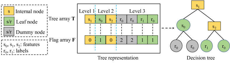
Figure 1: Representation of an example tree in GTree. The tree is represented with two arrays $\bm{T}$ and $\bm{F}$, where $|\bm{T}|=|\bm{F}|$. $\bm{T}[i]$ is an internal, leaf, or dummy node, and such information is marked as $\bm{F}[i]=0,1$, or $2$, respectively. $\bm{T}[i]$ is the assigned feature if it is an internal node, e.g., $\bm{T}[0]=s_{1}$ and $\bm{T}[2]=s_{2}$. For the dummy and leaf nodes in the last level, $\bm{T}[i]$ is the label of the path, e.g., $\bm{T}[3]=r_{0}$ and $\bm{T}[5]=r_{1}$; otherwise, $\bm{T}[i]$ is a random feature, e.g., $\bm{T}[1]=s_{0}$ (it is indeed a leaf). Although $\bm{T}[3]$ and $\bm{T}[4]$ are dummy nodes, they play the role of a leaf and store the label of their paths since they are in the last level. Such design not only protects the tree shape but also enables GTree to train and infer data in a highly parallelized manner.

IV-B Model Representation

As shown in Fig. 1, GTree uses an array $\bm{T}$ to represent a binary tree, where $\bm{T}[0]$ is the root node, $\bm{T}[2i+1]$ and $\bm{T}[2i+2]$ are the left and right children of $\bm{T}[i]$, respectively, and $0\leq i\leq|\bm{T}|/2-1$. The tree array has an auxiliary array $\bm{F}$, where $|\bm{F}|=|\bm{T}|$ and $\bm{F}[i]$ indicates the node type of $\bm{T}[i]$. $\bm{T}[i]$ represents a tree node, which could be an internal, leaf, or dummy node, and such information is marked as $\bm{F}[i]=0,1,2$, respectively. Specifically, $\bm{T}[i]$ is the assigned feature if it is an internal node. For the dummy and leaf nodes in the last level, $\bm{T}[i]$ is the label of the path (i.e., label $r_{0}$ and $r_{1}$ in Fig. 1); otherwise, $\bm{T}[i]$ is a random feature (e.g., $s_{0}$ in Fig. 1). Such design enables GTree to train and infer data in a highly parallelised manner.

By padding the model into a complete binary tree with dummy nodes, all the paths have the same length. As a result, no matter which path is taken during the training and inference, the processing time will always be the same. Since the model is a complete binary tree, the size of $T$ is determined by the depth. The depth of the tree is normally unknown before the training, yet $|\bm{T}|$ should be determined. To address this issue, we initialize $|\bm{T}|$ with the maximum value, i.e., $|\bm{T}|=2^{d}-1$. In case the tree depth $h$ is predefined, $|\bm{T}|=2^{h}-1$. $T$ is initialized with $|\bm{T}|$ leaves. Both $T$ and $F$ are shared among the three CSPs with RSS.

V Construction Details of GTree

In this section, we first present one basic block about how the CSPs access arrays jointly and obliviously without learning the access pattern. We then describe how GTree obliviously processes the 3 steps of DT training: learning phase, heuristic computation, and node split. Finally, we present the details of privacy-preserving DT inference. In the rest of this paper, we will use the symbols shown in Table II to represent the protocols designed for GTree.

TABLE II: Acronyms of protocols in GTree

Acronyms	Protocols
${\prod}_{\rm EQ}$ section A-A	Equality Test
${\prod}_{\rm OAA}$ section V-A	Oblivious Array Access
${\prod}_{\rm OL}$ section V-B1, section V-B2	Oblivious Learning
${\prod}_{\rm OHC}^{sgx}$/${\prod}_{\rm OHC}^{mpc}$ section V-B3	Oblivious Heuristic Computation via SGX/MPC
${\prod}_{\rm ONS}$ section V-B4	Oblivious Node Split
${\prod}_{\rm ODTT}$ section V-B5	Oblivious Decision Tree Training
${\prod}_{\rm ODTI}$ section V-C	Oblivious Decision Tree Inference

V-A Oblivious Array Access

To take advantage of GPU’s parallelism, GTree represents both the tree and data samples with arrays. During the training or inference, the array access pattern should be protected from the CSPs. Although they are all protected with RSS, the access pattern is still leaked if the CSPs are allowed to directly access the shares of the target element. There are two commonly used techniques to conceal access patterns: linear scan and ORAM. Considering the basic construction of linear scan involves a majority of highly parallelizable operations such as vectorized arithmetic operations, here we construct our Oblivious Array Access protocol ${\prod}_{\rm OAA}$ based on the linear scan, where the 3 CSPs jointly scan the whole array and obliviously retrieve the target element with an RSS-protected index.

1

Input : $\langle\bm{W}\rangle^{A}$ and $\langle\bm{U}\rangle^{A}$ (stores the target indices)

Output : All parties learn the shares of target elements $\langle\bm{Z}\rangle^{A}=\{\langle\bm{W}[u]\rangle^{A}\}_{\forall u\in\bm{U}}$

2

3Parties initialize an array $\langle\bm{O}\rangle^{A}$ with $|\bm{W}|$ zero values

4 for each $\langle u\rangle^{A}\in\langle\bm{U}\rangle^{A}$ do

5      

6      $\langle\bm{E}\rangle^{B}\leftarrow{\prod}_{\rm EQ}(\{\langle u\rangle^{A}\}^{|\bm{W}|},\{0,{\cdots},|\bm{W}|-1\})$

7       $\langle\bm{O}\rangle^{A}\leftarrow\mathtt{SelectShare}(\langle\bm{O}\rangle^{A},\langle\bm{W}\rangle^{A},\langle\bm{E}\rangle^{B})$

8       Compute $\langle z_{u}\rangle^{A}={\sum}_{k=0}^{|\bm{W}|-1}\langle\bm{O}[k]\rangle^{A}$

9      

10Output $\langle\bm{Z}\rangle^{A}=\{\langle z_{u}\rangle^{A}\}_{\forall u{\in}\bm{U}}$

Algorithm 1 Oblivious Array Access, ${\prod}_{\rm OAA}$

Equality test: ${\prod}_{\rm OAA}$ needs to obliviously check the equality between two operands or arrays with their shares. We modified the Less Than protocol in Rabbit [29] to achieve that, denoted as $\langle e\rangle^{B}\leftarrow{\prod}_{\rm EQ}(\langle x\rangle^{A},\langle y\rangle^{A})$. Specifically, $e=1$ if $x=y$; otherwise $e=0$. In particular, $\langle\bm{E}\rangle^{B}\leftarrow{\prod}_{\rm EQ}(\langle\bm{X}\rangle^{A},\langle\bm{Y}\rangle^{A})$ means compare the elements in the same index of two arrays, and $\bm{E}[i]=1$ if $\bm{X}[i]=\bm{Y}[i]$ (otherwise $\bm{E}[i]=0$), where $i\in[0,|\bm{X}|-1]$. Notably, one of the inputs can be public (e.g., $y$ or $\bm{Y}$), not the share. For more details, see Algorithm 8 in Appendix A-A.

Oblivious Array Access: Algorithm 1 illustrates our ${\prod}_{\rm OAA}$. Given the shares of the array $\bm{W}$ and the shares of a set of target indices $\bm{U}$, it outputs the shares of all the target elements. When $|\bm{U}|>1$, the target elements are accessed independently. Here we introduce how the three parties access one target element obliviously. Assume the target index is $\langle u\rangle^{A}$, parties first compare it with each index of $\bm{W}$ using ${\prod}_{\rm EQ}$ and get Boolean shares of the $|\bm{W}|$ comparison results: $\langle\bm{E}\rangle^{B}$ (Line 1). According to ${\prod}_{\rm EQ}$, only $\bm{E}[u]=1$, whereas that is hidden from the three parties as they only have the shares of $\bm{E}$. Second, the three parties use $\mathtt{SelectShare}$  to obliviously select elements from two arrays $\bm{W}$ and $\bm{O}$ based on $\langle\bm{E}\rangle^{B}$(Line 1), where $\bm{O}$ is an assistant array and contains $|\bm{W}|$ zeros. Since only $\bm{E}[u]=1$, after executing $\mathtt{SelectShare}$, we have $\bm{O}[u]=\bm{W}[u]$ and all the other elements of ${\bm{O}}$ are still 0. Finally, each party locally adds all the elements in $\langle\bm{O}\rangle^{A}$ and gets $\langle z_{u}\rangle^{A}$, where $z_{u}=\bm{W}[u]$ (Line 1). This algorithm can be processed in parallel with $|\bm{U}|*|\bm{W}|$ threads. Similarly, all the for-loops in the following protocols can be processed in parallel since the elements of arrays are processed independently.

V-B Oblivious DT Training

We summarise 3 steps for DT training in Section II-A. Here we present how GTree constructs oblivious protocols for them.

1

Input : $\langle\bm{D}\rangle^{A}$, $\langle\bm{T}\rangle^{A}$, $\langle\bm{F}\rangle^{A}$, $\langle\bm{M}\rangle^{A}$, $\{\langle\bm{C_{n}}\rangle^{A}\}_{n{\in}[0,n_{h}-1]}$ and current tree level $h$, where $n_{h}=2^{h}$ is the number of leaves at level $h$

Output : Updated $\{\langle\bm{C_{n}}\rangle^{A}\}_{n{\in}[0,n_{h}-1]}$

2

3if $h\neq 0$ then

4       $\langle\bm{Tval}\rangle^{A}\leftarrow{\prod}_{\rm OAA}(\langle\bm{T}\rangle^{A},\langle\bm{M}\rangle^{A})$

5       for $i=\{0,\cdots,N_{D}-1\}$ do

6             $\langle\bm{Dval}[i]\rangle^{A}\leftarrow{\prod}_{\rm OAA}(\langle\bm{D}[i]\rangle^{A},\langle\bm{Tval}\rangle^{A})$

7            

8      Compute $\langle\bm{M}\rangle^{A}=2\langle\bm{M}\rangle^{A}+\langle\bm{Dval}\rangle^{A}+1$

9      

10

11Initialize $\bm{LCidx}\leftarrow\{0,{\cdots},n_{h}-1\}$

12 $\langle\bm{isLeaf}\rangle^{B}\leftarrow{\prod}_{\rm EQ}(\{\langle\bm{F}[2^{h}-1]\rangle^{A},{\cdots},\langle\bm{F}[n_{h}+2^{h}-1]\rangle^{A}\},\{1\}^{n_{h}})$

13

14for $i=\{0,\cdots,N_{D}-1\}$ do

15       $\langle\bm{LCF}\rangle^{B}\leftarrow{\prod}_{\rm EQ}(\{\langle\bm{M}[i]\rangle^{A}-(2^{h}-1)\}^{n_{h}},\bm{LCidx}$)

16       $\langle\bm{LCF}\rangle^{B}~{}{\wedge}=~{}\langle\bm{isLeaf}\rangle^{B}$

17       Initialize $n_{h}$ $\bm{C}$ arrays for each data: $\langle\bm{C^{\prime}}_{D_{i}}\rangle^{A}\leftarrow\{\langle\bm{C^{\prime}_{\rho}}\rangle^{A}\}_{{\rho}{\in}[0,n_{h}-1]}$

18       for $\rho=\{0,\cdots,n_{h}-1\}$ do

19             for $k=\{0,\cdots,d-2\}$ do

20                   $\langle\bm{C^{\prime}_{\rho}}[0][2k]\rangle^{A}=(1-\langle\bm{D}[i][k]\rangle^{A})$

21                   $\langle\bm{C^{\prime}_{\rho}}[0][2k+1]\rangle^{A}=\langle\bm{D}[i][k]\rangle^{A}$

22                   $\langle\bm{C^{\prime}_{\rho}}[1][2k]\rangle^{A}=(1-\langle\bm{D}[i][k]\rangle^{A}){\cdot}(1-\langle\bm{D}[i][d-1]\rangle^{A})$

23                   $\langle\bm{C^{\prime}_{\rho}}[1][2k+1]\rangle^{A}=\langle\bm{D}[i][k]\rangle^{A}{\cdot}(1-\langle\bm{D}[i][d-1]\rangle^{A})$

24                   $\langle\bm{C^{\prime}_{\rho}}[2][2k]\rangle^{A}=(1-\langle\bm{D}[i][k]\rangle^{A}){\cdot}\langle\bm{D}[i][d-1]\rangle^{A}$

25                   $\langle\bm{C^{\prime}_{\rho}}[2][2k+1]\rangle^{A}=\langle\bm{D}[i][k]\rangle^{A}{\cdot}\langle\bm{D}[i][d-1]\rangle^{A}$

26                  

27            

28      $\langle\bm{C^{\prime}}_{D_{i}}\rangle^{A}{\leftarrow}\mathtt{SelectShare}(\{\langle 0\rangle^{A}\}^{n_{h}},\langle\bm{C^{\prime}}_{D_{i}}\rangle^{A},\langle\bm{LCF}\rangle^{B})$

29      

30Accumulate all $\{\langle\bm{C^{\prime}}_{D_{i}}\rangle^{A}\}_{i\in[0,N_{D}-1]}$ and output final $\{\langle\bm{C_{n}}\rangle^{A}\}_{n{\in}[0,n_{h}-1]}$.

Algorithm 2 Oblivious Learning, ${\prod}_{\rm OL}$

V-B1 Oblivious Learning: Data Partition

Algorithm 2 illustrates details of the learning phase of DT training. The first step is to partition the data samples into new leaves (Line 2-2). GTree uses an array $\bm{M}$ to indicate the leaf each data sample currently belongs to, where $\bm{M}[i]$ is the leaf identifier of $\bm{D}[i]$ and $|\bm{M}|=|\bm{D}|$, e.g., $\bm{M}[i]=n$ if $\bm{D}[i]$ is at $\bm{T}[n]$. Assume the new internal node is $\bm{T}[n]$ (which was a leaf and had a number of data samples) and the feature assigned to it is $s_{j}$. The main operation of data partition is to check if $\bm{D}[i][j]=0$ for each data sample at $\bm{T}[n]$. If yes, $\bm{D}[i]$ should be partitioned to the left child and $\bm{M}[i]\leftarrow 2\bm{M}[i]+1$ (i.e., $2n+1$); otherwise $\bm{M}[i]\leftarrow 2\bm{M}[i]+2$ (i.e., $2n+2$). That is, $\bm{M}[i]\leftarrow 2\bm{M}[i]+\bm{D}[i][j]+1$ (Line 2). To avoid leaking which leaf each data sample belongs to, GTree partitions the data samples obliviously.

GTree processes the leaves at the same level in parallel. So for the data partition, we first get the features assigned to new internal nodes at level $h-1$ from $\bm{T}$, the identifiers of which are stored in $\bm{M}$ as they previously were leaves. Parties thus run ${\prod}_{\rm OAA}(\langle\bm{T}\rangle^{A},\langle\bm{M}\rangle^{A})$ to get all such features (Line 2). The second step is to get the corresponding feature values from each data sample (Line 2), and then assign $\bm{M}$ with the new leaf identifiers based on the fetched feature values (Line 2). Notably, the values of $\bm{M}$ should be 0 if $h=0$.

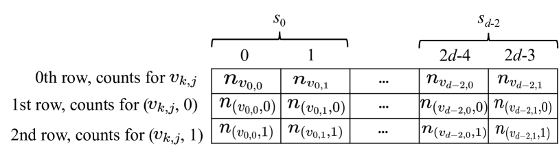
Figure 2: Counter array in GTree, denoted as $\bm{C}$. The array contains 3 rows and $2(d-1)$ columns. $C[0][2k+j]$ in the first row stores the number of data samples containing $v_{k,j}$, where $k\in[0,d-2]$ and $j\in\{0,1\}$. In the last two rows, $\bm{C}[1][2k+j]$ and $\bm{C}[2][2k+j]$ stores counts of $(v_{k,j},0)$ and $(v_{k,j},1)$ pairs, respectively. Such design also helps to take better advantage of GPU’s parallelism.

V-B2 Oblivious Learning: Statistics Counting

Statistics information of the data samples at each leaf is required for heuristic measurement. Specifically, for each real leaf, it requires the number of data samples containing each feature value and the number of data samples containing each (value, label) pair. GTree uses a 2D-array $\bm{C}$ to store such statistics for each leaf. As shown in Fig. 2, $\bm{C}$ has 3 rows and $2(d-1)$ columns (i.e., the total number of feature values). Particularly, the $2k$-th and $(2k+1)$-th elements of each row are the statistics of feature $s_{k}$, where $0{\leq}k{\leq}(d-2)$. Each element in the first row $\bm{C}[0][2k+j]$ stores the number of data samples containing the corresponding feature value $v_{k,j}$, where $j{\in}\{0,1\}$. In the last two rows, $\bm{C}[1][2k+j]$ and $\bm{C}[2][2k+j]$ stores counts of $(v_{k,j},0)$ and $(v_{k,j},1)$ pairs, respectively.

After assigning data samples to new leaves, GTree updates $\bm{C}$ of all leaves by scanning the partitioned data samples (Line 2-2). To hide the data samples’ distribution over leaves (i.e., the statistical information), GTree obliviously updates $\bm{C}$ of all leaves when processing each $\bm{D}[i]$. Indeed, only the real leaf that really contains $\bm{D}[i]$ should update its $\bm{C}$. To ensure the correctness of the final $\bm{C}$, a flag array $\bm{LCF}$ is used to indicate which $\bm{C}$ should be updated, and $\bm{LCF}$ contains two points: which leaf $\bm{D}[i]$ belongs to (Line 2), and if this leaf is real (Line 2, 2). Whether each element of $\bm{C}$ increases 1 or not depends on the feature values of $\bm{D}[i]$ (see Line 2-2), and GTree stores such information in a temporary counter array $\bm{C^{\prime}}_{\rho}$ and finally accumulates them in batch (Line 2).

V-B3 Oblivious Heuristic Computation

We next need to convert each leaf into an internal node using the best feature. For each path, a feature can only be assigned once, and GTree uses an array $\bm{\gamma}$ of size $d-1$ to indicate if each feature has been assigned or not. Specifically, $\bm{\gamma}[i]=0$ if $s_{i}$ has been assigned; otherwise $\bm{\gamma}[i]=1$.

We adopt gini index in heuristic computation (HC) due to its integer-arithmetic-friendly operations such as addition and multiplication. The Equation 1 can be distilled into the following equation based on $\bm{C}$, where $m_{k}=\bm{C}[k+1][2i+v_{i,0}]+\bm{C}[k+1][2i+v_{i,1}]$:

$$\footnotesize\begin{split}&\overline{G}(\bm{C},s_{i})={\sum}_{j=0}^{|\bm{V_{s_{i}}}|-1}\frac{P}{Q}\\ &P=(\bm{C}[0][2i+v_{i,j}])^{2}-{\sum}_{k=0}^{|\bm{V}_{s_{d-1}}|-1}{m_{k}}^{2}\\ &Q=\bm{C}[0][2i+v_{i,j}]{\cdot}(\bm{C}[0][2i+v_{i,0}]+\bm{C}[0][2i+v_{i,1}])\end{split}$$ (2)

We represent the gini index as a rational number, where $P$ and $Q$ are the numerator and denominator of Equation 2, respectively. Since there is an affine transformation between the fractions $\frac{P}{Q}$ and the gini index, minimizing the gini index is equivalent to minimizing $\frac{P}{Q}$. To find the best feature, we need to select the feature with the smallest gini index value by comparing $\frac{P}{Q}$ of different features. Naïvely, we can avoid expensive division by comparing the fractions of two features directly [21]: given non-negative $a,b,c,d$, we have that $\frac{a}{b}<\frac{c}{d}$ iff $a{\cdot}d<b{\cdot}c$. Nevertheless, such a solution imposes the restrictions on the modulus $2^{l}$ and the dataset size. Specifically, given all features are binary, the numerator and denominator are upper bounded by $N_{D}^{3}/8$ and $N_{D}^{2}/4$, respectively. In this case, the modulus must be at least $5{\cdot}(\log N_{D}-1)$ bits long. Therefore, $N_{D}$ can be at most $2^{13}=8,192$ for the modulus $2^{64}$ , which means we can process at most $8,192$ samples. Moreover, a larger modulus results in performance degradation. To our knowledge, this restriction is still an open obstacle to MPC-based secure DT training. In more recent work, Abspoel et al. [1] use the random forest instead of DT to bypass this limitation. To avoid the limitation of dataset size, we provide an MPC-only solution, namely MPC-based HC: ${\prod}_{\rm OHC}^{mpc}$.

1

Input : $\{\langle\bm{C_{n}}\rangle^{A}\}_{n{\in}[0,n_{h}-1]}$, $\{\langle\bm{\gamma_{n}}\rangle^{A}\}_{n{\in}[0,n_{h}-1]}$, $\langle\bm{F}\rangle^{A}$ and current tree level $h$

Output : Split decisions array $\langle\bm{SD}\rangle^{A}$ and updated $\{\langle\bm{\gamma_{n}}\rangle^{A}\}_{n{\in}[0,n_{h}-1]}$, $\langle\bm{F}\rangle^{A}$

2

3for $\rho=\{0,\cdots,n_{h}-1\}$ do

4       for $i=\{0,\cdots,d-2\}$ do

5             Compute $\langle\bm{P}[i]\rangle^{A}$ and $\langle\bm{Q}[i]\rangle^{A}$ using $\langle\bm{C_{t}}\rangle^{A}$ according to Equation 2

6             $\langle\bm{gini}[i]\rangle^{A}\leftarrow\mathtt{Division}(\langle\bm{P}[i]\rangle^{A},\langle\bm{Q}[i]\rangle^{A})$

7            

8      $\langle\bm{gini}\rangle^{A}\leftarrow\mathtt{SelectShare}(\langle\bm{O}\rangle^{A},\langle\bm{gini}\rangle^{A},{\prod}_{\rm EQ}(\langle\bm{\gamma_{\rho}}\rangle^{A},\{1\}^{d-1}))$

9       $\langle\bm{SD}[\rho]\rangle^{A}\leftarrow\mathtt{Maxpool}(\langle\bm{gini}\rangle^{A})$

10       $\langle\bm{\gamma_{\rho}}\rangle^{A}\leftarrow\mathtt{SelectShare}(\langle\bm{\gamma_{\rho}}\rangle^{A},\langle\bm{O}\rangle^{A},{\prod}_{\rm EQ}(\langle\bm{\gamma_{\rho}}\rangle^{A},\{\langle\bm{SD}[\rho]\rangle^{A}\}^{d-1}))$

11       $\langle\bm{F}[2\rho+2^{h+1}-1]\rangle^{A}\leftarrow\mathtt{SelectShare}(\langle 2\rangle^{A},\langle 1\rangle^{A},{\prod}_{\rm EQ}(\langle\bm{F}[\rho+2^{h}-1]\rangle^{A},2))$

12       $\langle\bm{F}[2\rho+2^{h+1}]\rangle^{A}=\langle\bm{F}[2\rho+2^{h+1}-1]\rangle^{A}$

13       $\langle\bm{F}[\rho+2^{h}-1]\rangle^{A}\leftarrow\mathtt{SelectShare}(\langle 0\rangle^{A},\langle 1\rangle^{A},{\prod}_{\rm EQ}(\langle{\Psi}_{r_{0}}\rangle^{A},0)~{}{\wedge}$ $~{}{\prod}_{\rm EQ}(\langle{\Psi}_{r_{1}}\rangle^{A},0)~{}{\wedge}~{}{\prod}_{\rm EQ}(\langle\bm{F}[\rho+2^{h}-1]\rangle^{A},1))$

14      

Algorithm 3 Oblivious Heuristic Computation via MPC, ${\prod}_{\rm OHC}^{mpc}$

MPC-based HC. ${\prod}_{\rm OHC}^{mpc}$ resorts to the relatively expensive MPC protocol $\mathtt{Division}$ to compute $\frac{P}{Q}$, and then uses $\mathtt{Maxpool}$ to compare the results of the fractions and select the best feature with the smallest gini index. We use the $\mathtt{Division}$ and $\mathtt{Maxpool}$ proposed in Falcon [51].

The gini index value is usually a real value (i.e., floating-point) while our MPC protocols are restricted to computations over discrete domains such as rings and finite fields. Similar to previous works [45, 34, 51], we use a fixed-point encoding strategy. In details, a real value $x{\in}\mathbb{R}$ is converted into an integer ${\lfloor}x{\cdot}2^{\tau}{\rceil}$ (i.e., the nearest integer to $x{\cdot}2^{\tau}$) with $\tau$ bits of precision. The value of $\tau$ affects both the performance and the inference accuracy. A smaller fixed-point precision enables to work with shares over a $32$-bit ring as opposed to a $64$-bit ring, thus reducing communication and computation costs. However, we might get the wrong best features since their gini index values with smaller fixed-point precision might become the same, which might affect the inference accuracy. Therefore, we need to carefully set a value for $\tau$ with experiments.

The detail of ${\prod}_{\rm OHC}^{mpc}$ is given in Algorithm 3, and it contains 3 main steps:

• For each path $\rho$, to hide the usage of features, the CSPs first jointly compute the gini index of all features with $\mathtt{Division}$ and obliviously select the unused feature with the minimum gini index as the best one with $\mathtt{Maxpool}$. Each CSP stores the share of the best feature in $\langle\bm{SD}\rangle^{A}$(Line 1-6).

• Since the selected feature cannot be assigned to other nodes in the same path, for each path $\rho$, the CSPs obliviously set $\bm{\gamma}_{\rho}[SD[\rho]]=0$ with $\mathtt{SelectShare}$ (Line 7) and the assistant array $\bm{O}$.

• $\bm{F}$ should also be updated since we will split the leaf into the internal node and generate new leaves. Note that, for leaf $\rho$, its index in $\bm{F}$ is $\rho+2^{h}-1$, and its children indices are $2\rho+2^{h+1}-1$ and $2\rho+2^{h+1}$. The children of a dummy node are also dummy, so $\bm{F}[2\rho+2^{h+1}-1]$ and $\bm{F}[2\rho+2^{h+1}]$ are obliviously set to 1 or 2 based on $\bm{F}[\rho+2^{h}-1]$. When all the data samples at leaf $\rho$ contain the same label, the training for this path is actually finished, and $\bm{F}[\rho+2^{h}-1]$ is set to 1. Otherwise, $\rho$ is converted into an internal node by setting $\bm{F}[\rho+2^{h}-1]=0$ (Line 8-10). Note that ${\Psi}_{r_{0}}$ and ${\Psi}_{r_{1}}$ in Line 3 are the number of data samples at the processing leaf containing $c_{0}$ and $c_{1}$, respectively.

As shown in CryptGPU [45], $\mathtt{Division}$ is unfriendly to GPU, and the HC process still cannot avoid $\mathtt{Division}$ operations. How to make $\mathtt{Division}$ operation GPU-friendly and how to avoid division for DT training are still an open challenge. To improve the performance, we alternatively propose to outsource the HC process to TEEs and present SGX-based HC: ${\prod}_{\rm OHC}^{sgx}$.

1

Input : $\{\langle\bm{C_{n}}\rangle^{A}\}_{n{\in}[0,n_{h}-1]}$, $\{\langle\bm{\gamma_{n}}\rangle^{A}\}_{n{\in}[0,n_{h}-1]}$, $\langle\bm{F}\rangle^{A}$ and current tree level $h$

Output : Split decisions array $\langle\bm{SD}\rangle^{A}$ and updated $\{\langle\bm{\gamma_{n}}\rangle^{A}\}_{n{\in}[0,n_{h}-1]}$, $\langle\bm{F}\rangle^{A}$

2

3$\{\bm{C_{n}}\}_{n{\in}[0,n_{h}-1]}=\mathtt{Reconstruct}^{A}(\{\langle\bm{C_{n}}\rangle^{A}\}_{n{\in}[0,n_{h}-1]})$

4 $\{\bm{\gamma_{n}}\}_{n{\in}[0,n_{h}-1]}=\mathtt{Reconstruct}^{A}(\{\langle\bm{\gamma_{n}}\rangle^{A}\}_{n{\in}[0,n_{h}-1]})$

5 $\bm{F}=\mathtt{Reconstruct}^{A}(\langle\bm{F}\rangle^{A})$

6 for $\rho=\{0,\cdots,n_{h}-1\}$ do

7       for $i=\{0,\cdots,d-2\}$ do

8             $\bm{gini}[i]=\overline{G}(\bm{C}_{\rho},s_{i})$

9            

10      $\bm{SD}[\rho]=\mathtt{oless}(\bm{gini},\bm{\gamma_{\rho}})$

11       $\mathtt{oassign}(\bm{\gamma_{\rho}},0,\bm{SD}[\rho])$

12       $\bm{F}[2\rho+2^{h+1}-1]=\mathtt{oselect}(2,1,\bm{F}[\rho+2^{h}-1]==2)$; $\bm{F}[2\rho+2^{h+1}]=\bm{F}[2\rho+2^{h+1}-1]$

13       Compute $CheckLeaf$ by checking if $\rho$-th node contains only one label

14       $\bm{F}[\rho+2^{h}-1]=\mathtt{oselect}(0,1,(\neg CheckLeaf\wedge(\bm{F}[\rho+2^{h}-1]==1)))$

15      

16$\langle\bm{SD}\rangle^{A}=\mathtt{Share}^{A}(\bm{SD})$

17 $\langle\bm{F}\rangle^{A}=\mathtt{Share}^{A}(\bm{F})$

18 $\langle\{\bm{\gamma_{n}}\}_{n{\in}[0,n_{h}-1]}\rangle^{A}=\mathtt{Share}^{A}(\{\bm{\gamma}_{n}\}_{n{\in}[0,n_{h}-1]})$

19 SGX sends the respective shares of the output arrays to the three GPUs

Algorithm 4 Oblivious Heuristic Computation via SGX, ${\prod}_{\rm OHC}^{sgx}$

SGX-based HC. ${\prod}_{\rm OHC}^{sgx}$ is shown in Algorithm 4. Basically, parties send the shares of all current $\{\bm{C_{n}},\bm{\gamma_{n}}\}_{n{\in}[0,n_{h}-1]}$ and $\bm{F}$ to the co-located SGX (assume on any of the three CSPs). The enclave reconstructs the inputs, generates or updates the 3 outputs based on the same principle as ${\prod}_{\rm OHC}^{mpc}$, and finally sends the respective shares of the outputs to each GPU. In particular, to avoid access pattern leakage, the enclave uses the following oblivious primitives (as done in [35, 25, 36]) to access all data inside the enclave:

• $\mathtt{oless}(\bm{vec},\bm{cond})$: compare values in $\bm{vec}$ and return the index of the minimum value. $\bm{cond}$ indicates which value in $\bm{vec}$ should not be compared.

• $\mathtt{oselect}(a,b,cond)$: conditionally select $a$ or $b$ based on condition $cond$.

• $\mathtt{oassign}(\bm{vec},a,idx)$: assign the value of $\bm{vec}$ at index $idx$ with $a$.

These oblivious primitives operate solely on registers whose contents are restricted to the code outside the enclave. Once the operands have been loaded into registers, the instructions are immune to memory-access-based pattern leakage.

Notably, other than computing the complex gini index, GTree also updates $\bm{F}$ and $\bm{\gamma}$ in sequence within the enclave because they are in small size and cannot benefit much from GPU acceleration.

1

Input : $\langle\bm{SD}\rangle^{A}$, $\langle\bm{F}\rangle^{A}$, $\{\langle\bm{C_{n}}\rangle^{A}\}_{n{\in}[0,n_{h}-1]}$ at level $h$

Output : Updated $\langle\bm{T}\rangle^{A}$, new arrays $\{\langle\bm{C_{n}}\rangle^{A}\}_{n{\in}[0,N_{c}-1]}$ at level $h+1$ where $N_{c}=2n_{h}$

2

3for $\rho=\{0,\cdots,n_{h}-1\}$ do

4       $\langle isInternal\rangle^{B}\leftarrow{\prod}_{\rm EQ}(\langle\bm{F}[\rho+2^{h}-1]\rangle^{A},0)$

5       for each $\langle\bm{C_{i}}\rangle^{A}$ in $\langle\bm{C^{\prime}_{\rho}}\rangle^{A}=\{\langle\bm{C_{i}}\rangle^{A}\}_{i{\in}[0,1]}\}$ do

6             $\langle\bm{C_{i}}\rangle^{A}{\leftarrow}\mathtt{SelectShare}(\langle\bm{C_{\rho}}\rangle^{A},\langle 0\rangle^{A},\langle isInternal\rangle^{B})$

7            

8      

9Concatenate all $\{\langle\bm{C^{\prime}_{\rho}}\rangle^{A}\}_{\rho\in[0,n_{h}-1]}$ into $\{\langle\bm{C_{n}}\rangle^{A}\}_{n{\in}[0,N_{c}-1]}$

10 Replace the values of $\langle\bm{T}\rangle^{A}$ at level $h$ with $\langle\bm{SD}\rangle^{A}$

Algorithm 5 Oblivious Node Split, ${\prod}_{\rm ONS}$

V-B4 Oblivious Node Split

The next step is to convert each leaf into an internal node using the best feature and generate new leaves at the next level (Algorithm 5). Recall that GTree builds the DT level by level. GTree updates $\bm{C}$ of all new leaves (Line 5-5) and $\bm{T}$ (Line 5) in parallel. In detail, the array $\bm{C}$ of a new leaf inherits from its parent node if the parent node is a dummy or leaf node; otherwise, set all values to zeros (Line 5). Notably, $\bm{\gamma}$ of each new leaf inherits from its parent node no matter which types the parent node is.

1

Input : $\langle\bm{D}\rangle^{A}$, public depth $H$

Output : $\langle\bm{T}\rangle^{A}$, $\langle\bm{F}\rangle^{A}$

2

3Parties initialize $\langle\bm{T}\rangle^{A}$, $\langle\bm{F}\rangle^{A}$, $\langle\bm{M}\rangle^{A}$, $\{\langle\bm{\gamma_{n}}\rangle^{A}\}_{n{\in}[0,n_{h}-1]}$ and $\{\langle\bm{C_{n}}\rangle^{A}\}_{n{\in}[0,n_{h}-1]}$, $n_{h}=1$

4

5for $h=\{0,\cdots,H-1\}$ do

6       $\{\langle\bm{C_{n}}\rangle^{A}\}_{n{\in}[0,n_{h}-1]}\leftarrow{\prod}_{\rm OL}(\langle\bm{D}\rangle^{A},\langle\bm{T}\rangle^{A},\langle\bm{F}\rangle^{A},\langle\bm{M}\rangle^{A},$

7       $\{\langle\bm{C_{n}}\rangle^{A}\}_{n{\in}[0,n_{h}-1]},h)$, $n_{h}=2^{h}$

8       $(\langle\bm{SD}\rangle^{A},\{\langle\bm{\gamma_{n}}\rangle^{A}\}_{n{\in}[0,n_{h}-1]},\langle\bm{F}\rangle^{A})\leftarrow{\prod}_{\rm OHC}^{sgx}/{\prod}_{\rm OHC}^{mpc}(\{\langle\bm{C_{n}}\rangle^{A}\}_{n{\in}[0,n_{h}-1]},$

9       $\{\langle\bm{\gamma_{n}}\rangle^{A}\}_{n{\in}[0,n_{h}-1]},\langle\bm{F}\rangle^{A},h)$

10       $(\{\langle\bm{C_{n}}\rangle^{A}\}_{n{\in}[0,N_{c}-1]},\langle\bm{T}\rangle^{A})\leftarrow{\prod}_{\rm ONS}(\langle\bm{SD}\rangle^{A},\langle\bm{F}\rangle^{B},\{\langle\bm{C_{n}}\rangle^{A}\}_{n{\in}[0,n_{h}-1]},h)$, $N_{c}=2^{h+1}$

11      

12for $i=\{0,\cdots,N_{c}-1\}$ do

13       $\langle\bm{T}[i+2^{h}-1]\rangle^{A}\leftarrow\mathtt{Maxpool}(\{\langle{\Psi}_{r_{0}}\rangle^{A},\langle{\Psi}_{r_{1}}\rangle^{A}\})$

14      

Algorithm 6 Oblivious Decision Tree Training, ${\prod}_{\rm ODTT}$

V-B5 Oblivious Decision Tree Training

The protocol of our privacy-preserving DT training is shown in Algorithm 6. GTree sequentially adds each entire level of the tree until up to a depth $H$ (Line 6-6). Finally, GTree obliviously select the label for each leaf or dummy node in the last level $h$ using $\mathtt{Maxpool}$ [51] (Line 6-6). Given the number of data samples containing each label, $\mathtt{Maxpool}$ returns the label with the largest counts. Within the algorithms 1-2 and 5-8, all the operations performed on arrays are executed concurrently with multiple threads, where each thread processes one element of the array.

As a result of such level-wise tree construction, GTree always build a full binary tree with a depth $H$. $H$ could be: (1) a pre-defined public depth; (2) a depth where all nodes at this level are leaf or dummy nodes; (3) a depth which is the number of features $d$ (including the label). Such design has a trade-off between privacy and performance. This is because we may add a lot of dummy nodes as the tree grows with deep depth, especially in the sparse DT.

V-C Oblivious DT Inference

1

Input : Unlabelled instance array $\langle\bm{I}\rangle^{A}$ of length $N_{I}$, $\langle\bm{T}\rangle^{A}$, tree depth $H$

Output : Inference result $\langle\bm{R}\rangle^{A}$ of length $N_{I}$

2

3Initialize $\langle\bm{Tidx}\rangle^{A}$, $\langle\bm{Tval}\rangle^{A}$ and $\langle\bm{Dval}\rangle^{A}$ of length $N_{I}$ with values to be zeros, $n_{iter}=0$

4 while $n_{iter}<H$ do

5       $\langle\bm{Tval}\rangle^{A}\leftarrow{\prod}_{\rm OAA}(\langle\bm{T}\rangle^{A},\langle\bm{Tidx}\rangle^{A})$

6       for $i=\{0,\cdots,N_{I}-1\}$ do

7             $\langle\bm{Dval}[i]\rangle^{A}\leftarrow{\prod}_{\rm OAA}(\langle\bm{I}[i]\rangle^{A},\langle\bm{Tval}\rangle^{A})$

8            

9      Compute $\langle\bm{Tidx}\rangle^{A}=2\langle\bm{Tidx}\rangle^{A}+\langle\bm{Dval}\rangle^{A}+1$

10       Compute $n_{iter}++$

11      

12$\langle\bm{R}\rangle^{A}=\langle\bm{Tval}\rangle^{A}$

Algorithm 7 Oblivious Decision Tree Inference, ${\prod}_{\rm ODTI}$

We describe the Oblivious Decision Tree Inference ${\prod}_{\rm ODTI}$ protocol in Algorithm 7. The main operation in ${\prod}_{\rm ODTI}$ is to obliviously access $\bm{T}$ and $\bm{I}$ (Line 7-7). The values of $\bm{T}$ at the last level $H$ are the inference results (Line 7). Notably, due to the benefits of GPU-friendly property in GTree, we can process a large number of concurrent queries. Considering ${\prod}_{\rm OAA}$ is oblivious, which node and feature value are really used for the inference in each level is hidden from CSPs, thus the tree access pattern during inference is also hidden in GTree.

VI Performance Evaluation

We build GTree on top of Piranha [53], a general-purpose modular platform for accelerating secret sharing-based MPC protocols using GPUs. Piranha provides some state-of-the-art secret-sharing MPC protocols that allow us to easily leverage GPU. Particularly, some of these protocols such as $\mathtt{SelectShare}$, $\mathtt{Division}$ and $\mathtt{Maxpool}$ [51] are used in GTree.

In this section, we evaluate the performance of GTree training and inference. We also compare the performance of GTree with previous CPU-based solutions and two baselines.

VI-A Experiment Setup

Testbed. We evaluate the prototype on a server equipped with 3 NVIDIA Tesla V100 GPUs, each of which has 32 GB of GPU memory. The server runs Ubuntu 20.04 with kernel version 5.4.0 and has 10-core Intel Xeon Silver 4210 CPUs (2.20GHz) and 125GB of memory. We implement GTree in C++ and marshal GPU operations via CUDA 11.6. Since the GPU server does not support Intel SGX, we use a desktop with SGX support to test SGX-based protocol. The desktop contains 8 Intel i9-9900 3.1GHZ cores and 32GB of memory (${\thicksim}93$ MB EPC memory) and runs Ubuntu 18.04.5 LTS and OpenEnclave 0.16.0 [30].

Network Latency. Although we test all the protocols on the same machine, Piranha provides the functionality to emulate the network connection and measure network latency based on the communication overhead and the bandwidth. Our test uses a local area network (LAN) environment with a bandwidth of 10 Gbps and ping time of 0.07 ms (same setting as [1, 21]). Since current GPU-GPU communication over the network is not widespread, communication between GPUs is bridged via CPU in Piranha [53]. GTree inherits this property. The time for transferring data between GPU and CPU on the same machine is negligible in GTree.

All the results presented in the following are average over 10 runs.

TABLE III: Datasets

Dataset	#Features	#Labels	#Samples	Tree Depth
SPECT	$22$	$2$	267	6
KRKPA7	$35$	$2$	3,196	9
Adult	$14$	$2$	48,842	5

VI-B Performance of GTree Training

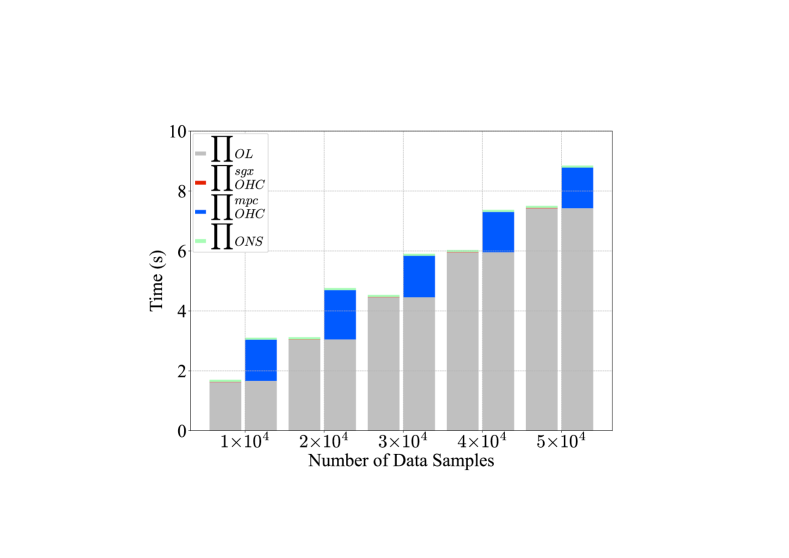
(a) With $8$ features and 6 tree depth

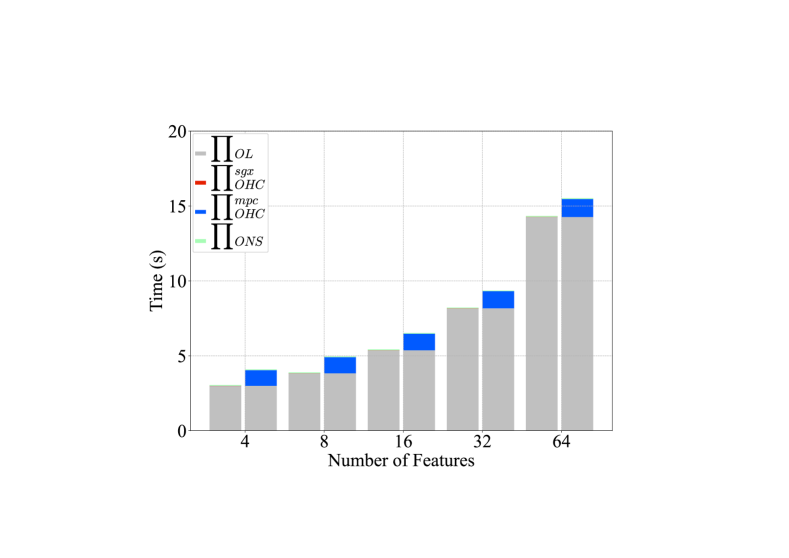
(b) With $50,000$ data samples and 5 tree depth

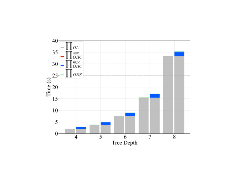
(c) With $8$ features and $50,000$ data samples

Figure 3: Performance of the three steps for DT training. The left and right bars of each case are the execution times of ${\prod}_{\rm ODTT}$ using ${\prod}_{\rm OHC}^{sgx}$ and ${\prod}_{\rm OHC}^{mpc}$, respectively.

We first evaluate the performance of the protocols used in DT training: ${\prod}_{\rm OL}$, ${\prod}_{\rm OHC}^{mpc}$, ${\prod}_{\rm OHC}^{sgx}$, and ${\prod}_{\rm ONS}$. For this test, we use a synthetic dataset which allows us to flexibly change the number of data samples, features, and depths so as to better show the performance of GTree under different conditions. The ML python package, scikit-learn , is employed to generate the data in our test. The results (including both computation and network latency) are shown in Fig. 3.

From Fig. 3 we can see that the learning phase is the most expensive step and the node split phase is very efficient. For example, for training $5{\times}10^{4}$ data samples with depth 8, GTree spends 33.24s and 0.11s on the learning phase and node split, respectively. The learning phase takes up about 98% of the runtime in training on average. The main reason is that this step uses ${\prod}_{\rm OAA}$ and $\mathtt{SelectShare}$ with a large input size (e.g., $N_{D}$) multiple times, which incurs heavy communication cost.

Heuristic Computation: ${\prod}_{\rm OHC}^{mpc}$ vs. ${\prod}_{\rm OHC}^{sgx}$. For the heuristic computation phase, as discussed in Section V-B3, in ${\prod}_{\rm OHC}^{mpc}$, the value of $\tau$ affects both the performance of ${\prod}_{\rm OHC}^{mpc}$ and the inference accuracy of the model. From our experiment results, we observe that when setting $\tau=10$ and working over the ring $\mathbb{Z}_{2^{32}}$, the inference accuracy of the model trained using ${\prod}_{\rm OHC}^{mpc}$ is acceptable. Thus, for evaluating ${\prod}_{\rm OHC}^{mpc}$, we set $\tau=10$.

For the inference accuracy of GTree when setting $\tau=10$, here we present the results tested with 3 real datasets that are widely used in the literature: SPECT Heart (SPECT) dataset, Chess (King-Rook vs. King-Pawn) (KRKPA7) dataset, Adult dataset (see the dataset information in Table III). The DT model trained with plaintext data achieves $71\%$, $81.1\%$ and $79.4\%$ accuracy on the SPECT, KRKPA7, and Adult datasets, respectively. The secure model trained by GTree using ${\prod}_{\rm OHC}^{sgx}$ achieves the same inference accuracy as the plaintext model. However, the secure model trained with ${\prod}_{\rm OHC}^{mpc}$ drops the inference accuracy to $68\%$, $62.3\%$, and $61.3\%$ for the three datasets, respectively.

The results indicate that, even with sufficient precision, accuracy loss can still occur. This is a common issue for MPC-protected ML systems, which is not limited to GTree and DT models. For DT, this can be attributed to 3 main factors: (i) given relatively big precision and large-size datasets, the numerator and denominator $P$ and $Q$ in Equation 2 become large, and scaling them (to avoid overflow and utilize the function provided in Piranha [53]) can lead to accuracy loss; (ii) $\mathtt{Division}$ utilizes the approximation technique (i.e., Taylor expansion [45, 51, 53]) which may introduce a certain degree of accuracy loss. (iii) the gini index values of different features can be very close, which can result in the selection of wrong features when comparing them under MPC.

When $\tau=10$, Fig. 3 shows that ${\prod}_{\rm OHC}^{sgx}$ outperforms ${\prod}_{\rm OHC}^{mpc}$ significantly. Precisely, by $136{\times}$ on average. Compared with ${\prod}_{\rm OL}$, the time taken by ${\prod}_{\rm OHC}^{sgx}$ is almost negligible. Overall, for training $5\times 10^{4}$ data samples, the system using ${\prod}_{\rm OHC}^{sgx}$ is ${\thicksim}1.3\times$ faster than the one using ${\prod}_{\rm OHC}^{mpc}$.

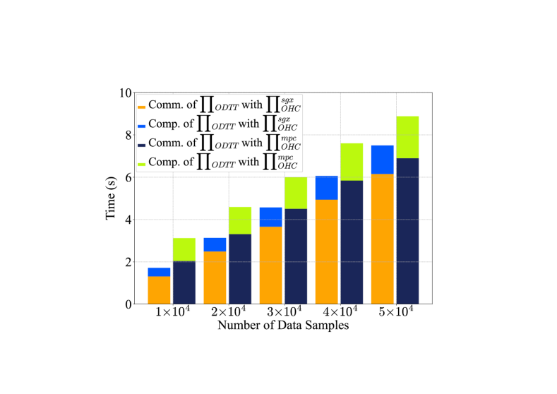
(a) With $8$ features and 6 levels

(b) With $50,000$ samples and 5 levels

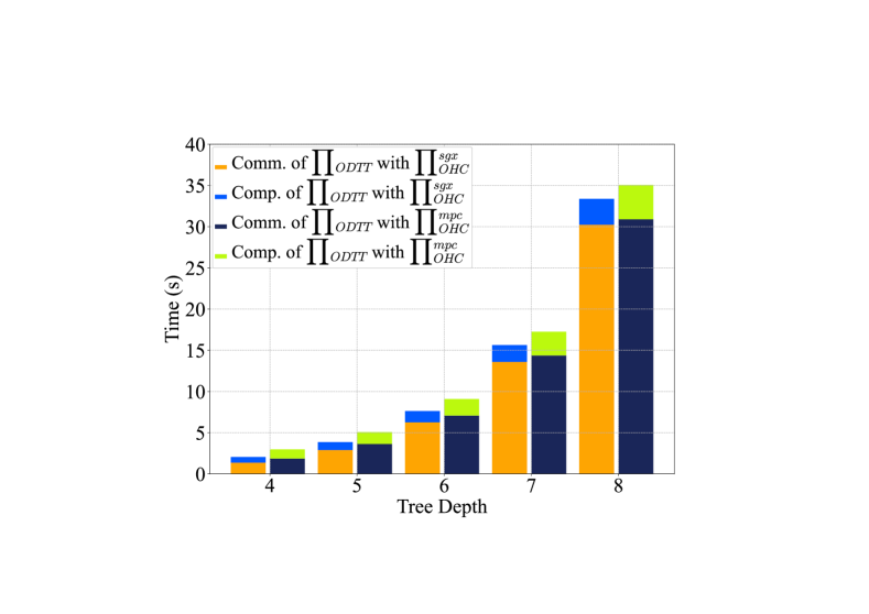
(c) With $8$ features and $50,000$ samples

Figure 4: Computation (Comp.) and Communication (Comm.) time of training.

TABLE IV: Comm. cost (MB) for different #features

#Features	4	8	16	32	64
${\prod}_{\rm OL}$	639	937	1531.6	2721.8	5102.2
${\prod}_{\rm OHC}^{sgx}$	0.004	0.008	0.016	0.031	0.061
${\prod}_{\rm OHC}^{mpc}$	0.277	0.553	1.11	2.21	4.42
${\prod}_{\rm OHC_{ONS}}$	0.011	0.02	0.04	0.079	0.157
${\prod}_{\rm ODTT}$ with ${{\prod}_{\rm OHC}^{sgx}}$	639.03	936.6	1531.7	2722	5102.4
${\prod}_{\rm ODTT}$ with ${{\prod}_{\rm OHC}^{mpc}}$	639.3	937.1	1532.8	2724	5106.8

TABLE V: Comm. cost (MB) for different depths

#Depths	4	5	6	7	8
${\prod}_{\rm OL}$	460.1	936.6	1924.9	3998.2	8363.4
${\prod}_{\rm OHC}^{sgx}$	0.004	0.008	0.017	0.034	0.070
${\prod}_{\rm OHC}^{mpc}$	0.258	0.553	1.14	2.32	4.68
${\prod}_{\rm OHC_{ONS}}$	0.009	0.020	0.041	0.084	0.170
${\prod}_{\rm ODTT}$ with ${{\prod}_{\rm OHC}^{sgx}}$	460.1	936.6	1925	3998.4	8363.6
${\prod}_{\rm ODTT}$ with ${{\prod}_{\rm OHC}^{mpc}}$	460.4	937.1	1926.1	4000.6	8368.3

Communication Overhead. The main issue of MPC is the heavy communication overhead. We measure the communication overhead for training in GTree with different numbers of features and tree depths ($5\times 10^{4}$ data samples), and the results are given in Table IV and V, respectively. As mentioned above, the learning phase has the most communication overhead as it takes a huge amount of data samples as inputs, which is also the dominant overhead of GTree training. For heuristic computation, the SGX-based protocol has much less communication than the MPC-based one.

In Fig. 4, we split the training time into the time spent on communicating and computing. With our LAN setting, about $69\%-90\%$ (also varies with the network bandwidth) overhead of GTree training is the communication among the 3 CSPs, which is similar to CryptGPU [45] and Piranha [53]. We will optimize the communication overhead in our future work. It is worth noting that even with heavy communication overhead, GTree is still highly more efficient than CPU-based and TEE-based solutions (see Section VI-D).

VI-C Performance of GTree Inference

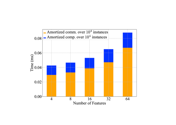
(a) With 5 tree depth

(b) With 10 features

Figure 5: Computation and communication time of inference.

To test inference, we input $10^{4}$ instances and measure the amortized time, which is broken down into computation and communication times, and the results are shown in Fig. 5. Similar to the training process, the main overhead of inference is also the communication, which takes about $69\%-90\%$ with our LAN setting.

Comparing Fig. 5(a) and Fig. 5(b), we can see the performance of DT inference is affected more significantly by the tree depth than the number of features, and when the tree depth $\geq 10$, the GTree inference time goes up sharply. Algorithm 7 shows that the DT inference mainly invokes ${\prod}_{\rm OAA}$ to process instances, and how many times ${\prod}_{\rm OAA}$ is invoked to process each instance depends on the tree depth $H$ ($N_{I}$ instances are processed in parallel). Thus, in terms of inference, GTree is more suitable for processing the trees with small or medium depths. For trees with large depths, we can refer to random forests.

VI-D Performance Comparisons with Others

TABLE VI: Training time in seconds

Scheme	SPECT	KRKPA7	Adult
$\mathtt{SID3T}$	3.55	6.45 (not secure)	89.07
GTree	0.31	8.63	4.32

Comparisons with Prior Work. We also compare the performance of GTree against Hoogh et al. [21] and Liu et al. [28]. To the best of our knowledge, these are the only private DT works that demonstrated the ability to train the dataset with categorical features in a relatively efficient manner. Several recent works [1, 2, 20] focus on designing specified MPC protocols (e.g., sorting) to process continuous features, we do not compare GTree with them.

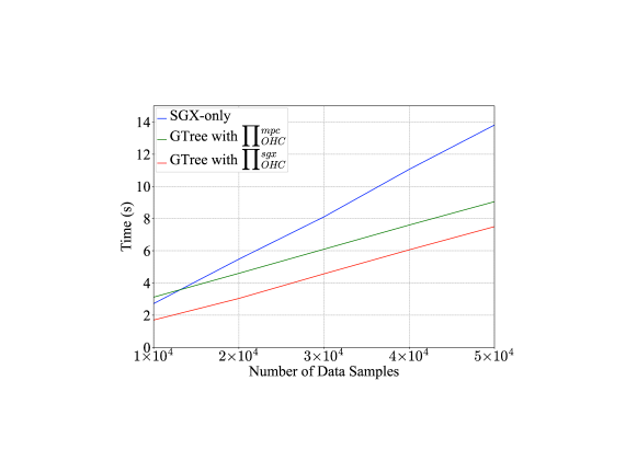
(a) Training, with 8 features and 6 levels

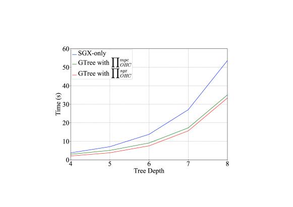
(b) Training, with 8 features and 50,000 data samples

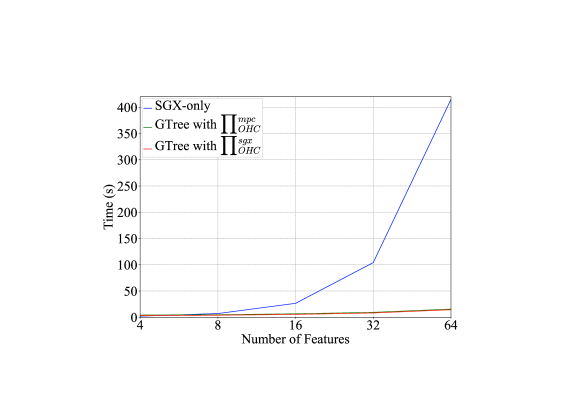
(c) Training, with 50,000 data samples and 5 levels

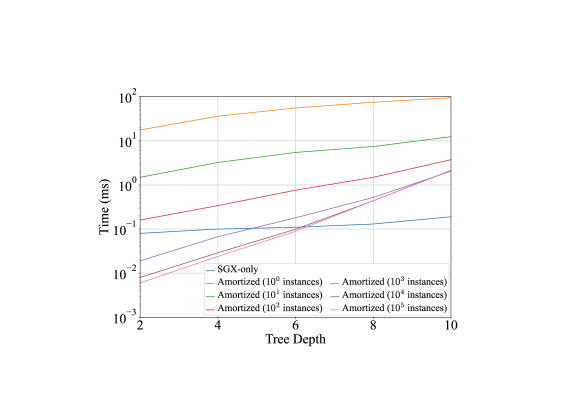
(d) Inference, with 10 features, $\mathtt{SGX~{}only}$ infers 1 instance

Figure 6: Performance of $\mathtt{SGX~{}only}$ and GTree for training and inference. Note that $y$-axis in Fig. 6(d) is in logarithm scale.

As described in most recent works [1, 2], the approach proposed in Hoogh et al. [21] is still the most state-of-the-art privacy-preserving DT work to process categorical features. They provide three protocols with different levels of security. We implement their protocol with the highest level of security on top of their latest efficient MPC framework: MPyC [42]. We denote this baseline as $\mathtt{SID3T}$. However, $\mathtt{SID3T}$ does not protect the shape of the tree, which is less secure than GTree. It is worth noting that in secure DT training, protecting the tree’s shape is typically one of the most challenging and expensive tasks.

We first evaluated the performance of DT training with the 3 datasets in Table VI. The details of each dataset are shown in Table III. The depths of the DT trained over these datasets are 6, 9, and 5 respectively. $\mathtt{SID3T}$ is tested on the CPU of the same machine used in GTree. The results are shown in Table VI. For SPECT and Adult, GTree outperforms $\mathtt{SID3T}$ by ${\thicksim}11{\times}$ and ${\thicksim}21{\times}$, respectively. When training with KRKPA7, GTree’s performance is slightly worse than $\mathtt{SID3T}$. This is because GTree trains a full binary tree up to the depth to protect the tree structure. Nevertheless, $\mathtt{SID3T}$ avoids such an expensive part at the expense of security loss. Overall, GTree demonstrates superior performance while providing stronger security.

We only provide a rough comparison between GTree and Liu et al. [28] by using the performance results reported in their paper, since their implementation is not publicly available at the time of writing. The largest dataset they used is the Tic-tac-toe dataset containing 958 data samples and 9 features. When training with this dataset , GTree takes 0.43 seconds and 39.61 MB communication cost, yielding ${\thicksim}3,112{\times}$ and ${\thicksim}49{\times}$ improvements. Notably, Liu et al. [28] also do not protect the tree structure.

TABLE VII: Inference time in milliseconds

Dataset	#Features	Depth	GGH [23]	GTree	Speedup
Wine	7	5	14	0.05	$280{\times}$
Breast	12	7	24	0.19	$126{\times}$
Digits	47	15	115	102.7	$1.1{\times}$

For DT inference, Kiss et al. [23] implement most of the existing private DT inference protocols and systematically compare their performance. In Table VII, we compare GTree with GGH proposed by Kiss et al. [23], the prior most efficient private DT inference protocol. The runtimes of GGH are read from their paper. For the 3 datasets included in Table VII, the inference times of GTree are amortized over $10^{4}$, $10^{4}$, and $10^{3}$ (due to GPU memory constraints) instances, respectively.

Comparisons with SGX-only Solution. As mentioned, protecting data processes with TEE is another research line in the literature. Although GPU itself cannot provide protection, due to its powerful parallelism capability, GPU is a better option to achieve a practical privacy-preserving DT system. Another reason is that existing TEEs, such as Intel SGX [11] and AMD SEV [4], suffer from side-channel attacks regardless of the provided confidentially and integrity guarantee. To protect the model effectively from side-channel attacks, the training and inference processes performed within TEEs should be oblivious, which is expensive. Here we use Intel SGX as an example and implement a prototype of DT system that processes everything inside an SGX enclave obliviously with oblivious primitives, e.g., $\mathtt{oassign}$ and $\mathtt{oaccess}$ [35, 25, 36]. The evaluation results are given in Fig. 6.

For training, Fig. 6(a),  6(b), and 6(c) show that GTree outperforms the SGX-only solution almost for all cases. For inference, SGX-only is much more efficient than GTree when inferring only one instance. However, the performance of GTree gets better when increasing the number of instances since GPU parallelism is getting better utilized, and when the tree depth is 10, it is fully utilized when concurrently inferring $10^{3}$ instances. When the tree depth is 6, the GPU-based solution GTree outperforms the SGX-only solution when inferring more than $10^{4}$ data instances concurrently, and the advantage of GTree is more obvious when the tree depth is less than 6. Note that the performance of GTree will be better with more powerful GPUs.

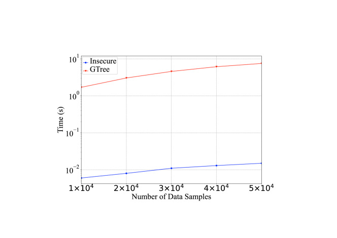
(a) With 8 features and 6 tree depth

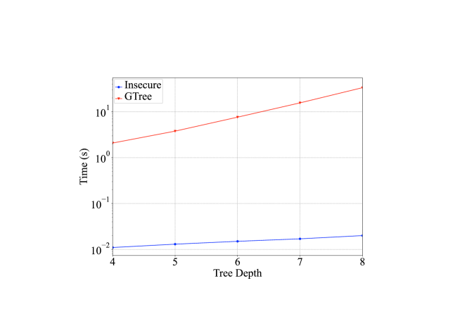
(b) With 8 features and 50,000 data samples

Figure 7: Training of $\mathtt{Insecure}$ and GTree. Note that $y$-axis is in logarithm scale.

Comparisons with Plaintext Training. As done in CryptGPU [45], in Fig. 7, we also report the comparison results between $\mathtt{Insecure}$ baseline and GTree, where $\mathtt{Insecure}$ baseline trains the same datasets in plaintext with one GPU. For CNN training, CryptGPU still adds roughly $2000\times$ overhead compared with the insecure training. For DT training with GTree, as shown in Fig. 7 (in appendix), the gap is less than $1673\times$. Even though, the gap between them is still large, which highlights the need for developing more GPU-friendly cryptographic primitives in the future.

VII Security Analysis

We prove the security of our protocols using the real-world/ideal-world simulation paradigm [18, 9, 8]. Let $\mathcal{A}$ denote the static semi-honest probabilistic polynomial time (PPT) real-world adversary, $\mathcal{S}$ denote the corresponding ideal-world adversary (a.k.a. simulator), and $\mathcal{F}$ denote the ideal functionality. The computationally bounded adversary $\mathcal{A}$ corrupts at most one party (i.e., $P_{1}$) at the beginning of the protocol and follows the protocol specification honestly. Security is modeled by defining two interactions [18, 51]: in the real world, $P_{1}$, $P_{2}$, and $P_{3}$ execute the protocol in the presence of $\mathcal{A}$ and the environment $\mathcal{Z}$; in the ideal world, the parties send their inputs to a trusted party that computes the functionality truthfully. Finally, to prove the security of our protocols, for every adversary $\mathcal{A}$ in the real world, there exists a simulator $\mathcal{S}$ in the ideal world such that no environment $\mathcal{Z}$ can distinguish between real and ideal world. This means that any information that the adversary $\mathcal{A}$ can extract in the real-world scenario can also be extracted by the simulator $\mathcal{S}$ in the ideal-world scenario.

We utilize multiple sub-protocols to design our protocols in the sequential model and employ the hybrid model for our security proofs. The hybrid model replaces sub-protocols with the invocation of instances of corresponding functionalities, thus it can simplify the proof analysis significantly. A protocol that invokes a functionality $\mathcal{F}$ is said to be in an “$\mathcal{F}$-hybrid model”.

We define the respective simulators $\mathcal{F}_{\rm EQ}$, $\mathcal{F}_{\rm OAA}$, $\mathcal{F}_{\rm OL}$, $\mathcal{F}_{\rm OHC}^{mpc}$, $\mathcal{F}_{\rm ONS}$, $\mathcal{F}_{\rm ODTT}$ and $\mathcal{F}_{\rm ODTI}$ for protocols ${\prod}_{\rm EQ}$, ${\prod}_{\rm OAA}$, ${\prod}_{\rm OL}$, ${\prod}_{\rm OHC}^{mpc}$, ${\prod}_{\rm ONS}$, ${\prod}_{\rm ODTT}$ and ${\prod}_{\rm ODTI}$. The ideal functionalities for multiplication and reconstruct ($\mathcal{F}_{\rm Mult}$ and $\mathcal{F}_{\rm Reconst}$) are identical to prior works [51, 39]. We prove security using the standard indistinguishability argument. To prove the security of a particular functionality, we set up hybrid interactions where the sub-protocols used in that protocol are replaced by their corresponding ideal functionalities. We then prove that these interactions can be simulated in a way that is indistinguishable from real interactions.

The following analysis and theorems give the indistinguishability of these two interactions.

Security of ${\prod}_{\rm EQ}$. In ${\prod}_{\rm EQ}$, we mainly modify Step 8 compared to the protocol in Rabbit [29], where the involved computations are all local. Therefore, the simulator for $\mathcal{F}_{\rm EQ}$ follows easily from the original protocol, which has been proved secure.

Security of ${\prod}_{\rm OAA}$. We capture the security of ${\prod}_{\rm OAA}$ as Themorem 1 and give the detailed proof as follows.

Theorem 1.

${\prod}_{\rm OAA}$ securely realizes $\mathcal{F}_{\rm OAA}$, in the presence of one semi-honest party in the ($\mathcal{F}_{\rm Mult}$, $\mathcal{F}_{\rm EQ}$, $\mathcal{F}_{\rm SelectShare}$)-hybrid model.

Proof.

The simulation follows easily from the protocol and the hybrid argument. The simulator runs the first iteration of the loop (Step 1) and in the process extracts the inputs. Then it proceeds to complete all the iterations of the loop. The simulator for $\mathcal{F}_{\rm EQ}$ can be used to simulate the transcripts from Step 1. The simulator for $\mathcal{F}_{\rm SelectShare}$ follows from the protocol in Falcon [51]. Steps 1 and  1 are all local operations and do not need simulation. Therefore, ${\prod}_{\rm OAA}$is secure in the ($\mathcal{F}_{\rm Mult}$, $\mathcal{F}_{\rm EQ}$, $\mathcal{F}_{\rm SelectShare}$)-hybrid model. ∎

Security of ${\prod}_{\rm OL}$. We capture the security of ${\prod}_{\rm OL}$ as Themorem 2 and give the detailed proof as follows.

Theorem 2.

${\prod}_{\rm OL}$ securely realizes $\mathcal{F}_{\rm OL}$, in the presence of one semi-honest party in the ($\mathcal{F}_{\rm Mult}$, $\mathcal{F}_{\rm EQ}$, $\mathcal{F}_{\rm OAA}$, $\mathcal{F}_{\rm SelectShare}$)-hybrid model.

Proof.

The simulator for $\mathcal{F}_{\rm Mult}$ can be used to simulate the transcripts from Steps 2, 2- 2. ${\prod}_{\rm OL}$ are sequential combinations of local computations (Steps 2, 2, 2, 2, 2, 2) and invocations of $\mathcal{F}_{\rm Mult}$, $\mathcal{F}_{\rm EQ}$ (Steps 2, 2), $\mathcal{F}_{\rm OAA}$ (Steps 2, 2) and $\mathcal{F}_{\rm SelectShare}$ (Step 2). The simulation follows directly from composing the simulators. ∎

Security of ${\prod}_{\rm OHC}^{mpc}$. Protocol ${\prod}_{\rm OHC}^{mpc}$ is composed of protocols such as $\mathtt{Division}$ and $\mathtt{Maxpool}$ from Falcon [51]. The security statement and proof of ${\prod}_{\rm OHC}^{mpc}$ are as follows:

Theorem 3.

${\prod}_{\rm OHC}^{mpc}$ securely realizes $\mathcal{F}_{OHC}^{mpc}$, in the presence of one semi-honest party in the ($\mathcal{F}_{\rm Mult}$, $\mathcal{F}_{\rm EQ}$, $\mathcal{F}_{\rm SelectShare}$, $\mathcal{F}_{\rm Maxpool}$, $\mathcal{F}_{\rm Division}$)-hybrid model.

Proof.

The simulators for $\mathcal{F}_{\rm Maxpool}$, $\mathcal{F}_{\rm Division}$ and $\mathcal{F}_{\rm SelectShare}$ follow from Falcon [51]. ${\prod}_{\rm OL}$ are sequential combinations of local computations and invocations of those corresponding simulators. ∎

Security of ${\prod}_{\rm OHC}^{sgx}$. We explain the ideal functionality for ${\prod}_{\rm OHC}^{sgx}$ according to the functionality $\mathcal{F}_{\rm attest}$ proposed in CRYPTFLOW [24]. $\mathcal{F}_{\rm OHC}^{sgx}$ is realized as follows: Intel SGX provides confidentiality guarantees by creating a secure enclave within the system’s memory where code and data can be securely executed and stored. In the beginning, when SGX receives a command for computing heuristic measurement, it performs a remote attestation with the party. Once attested, the data transmitted between the party and the enclave will be encrypted with a secret key $sk$. Now, on receiving the inputs from the parties, the enclave starts executing the code of HC and produces secret-shared outputs encrypted under $sk$. When running the code inside the enclave, even if an adversary compromises the host system, he cannot learn the data from the enclave.

Security of ${\prod}_{\rm ONS}$. We capture the security of ${\prod}_{\rm ONS}$ as Themorem 4 and give the detailed proof as follows.

Theorem 4.

${\prod}_{\rm ONS}$ securely realizes $\mathcal{F}_{\rm ONS}$, in the presence of one semi-honest party in the ($\mathcal{F}_{\rm EQ}$, $\mathcal{F}_{\rm SelectShare}$)-hybrid model.

Proof.

Similar to the proof of Theorem 2, simulation works by sequentially composing the simulators for $\mathcal{F}_{\rm EQ}$ and $\mathcal{F}_{\rm SelectShare}$. ∎

Security of ${\prod}_{\rm ODTT}$ and ${\prod}_{\rm ODTI}$. We capture the security of protocols ${\prod}_{\rm ODTT}$, and ${\prod}_{\rm ODTI}$ in respective 5, and 6, and give their formal proofs as follows:

Theorem 5.

${\prod}_{\rm ODTT}$ securely realizes $\mathcal{F}_{\rm ODTT}$, in the presence of one semi-honest party in the ($\mathcal{F}_{\rm OL}$, $\mathcal{F}_{\rm OHC}^{mpc}$/$\mathcal{F}_{\rm OHC}^{sgx}$, $\mathcal{F}_{\rm ONS}$)-hybrid model.

Proof.

Simulation is done using the hybrid argument. The protocol simply composes $\mathcal{F}_{\rm OL}$, $\mathcal{F}_{\rm OHC}^{mpc}$/$\mathcal{F}_{\rm OHC}^{sgx}$ and $\mathcal{F}_{\rm ONS}$ and hence is simulated using the corresponding simulators. ∎

Theorem 6.

${\prod}_{\rm ODTI}$ securely realizes $\mathcal{F}_{\rm ODTI}$, in the presence of one semi-honest party in the $\mathcal{F}_{\rm OAA}$-hybrid model.

Proof.

The simulation follows easily from the protocol and the hybrid argument. Simulation works by sequentially composing $\mathcal{F}_{\rm OAA}$ and hence is simulated using the corresponding simulator. ∎

VIII Related Work

In this section, we review existing privacy-preserving approaches for general ML algorithms and explore the most recent works that leverage GPU acceleration. We finally survey the work for privacy-preserving DT training and inference.

VIII-A Privacy-preserving machine learning using GPU

Privacy-preserving ML has received considerable attention over recent years. Recent works operate in different models such as deep learning [39, 51, 35, 33, 50, 40, 27] and tree-based models [1, 2, 28, 25, 26, 16, 21, 47, 56, 44]. These works rely on different privacy-preserving techniques, such as MPC [39, 51, 50, 40, 1, 2, 26, 16, 21, 47, 56], HE [28, 44], TEE [35, 25] or a combination of several of these techniques [33, 27]. However, most of them demonstrate a CPU-only implementation and focus mainly on improving the performance of their specified protocols. There is a broad and pressing call to improve the practical performance further when deploying them on real-life applications.

In recent years, few works have explored GPU-assisted MPC in privacy-preserving deep learning. Two earliest works [17, 22] leverage GPU to speed up some basic operations in MPC. Delphi [31] explores the use of GPU for improving the performance of linear layers. CryptGPU [45] shows the benefits of GPU acceleration for both training and inference on top of the CrypTen framework. GForce [34] proposes an online/offline GPU/CPU design for inference with GPU-friendly protocols. Visor [36] is the first to combine the CPU TEE with GPU TEE in video analytics, yet it is closed-source. Moreover, GPU TEE [49] requires hardware modification which would adversely affect compatibility. Overall, all of these works focus on deep learning due to massive GPU-friendly computations (i.e., convolutions and matrix multiplications). GTree is the first to support secure DT training and inference on the GPU.

VIII-B Privacy-preserving Decision Tree

Inference. Most of the existing works [7, 54, 14, 47, 56, 44, 6, 25, 35] focus mainly on DT inference. Given a pre-trained DT model, they ensure that the QU (or say client) learns as little as possible about the model and the CSP learns nothing about the queries. Among these works, SGX-based approaches [25, 35] have demonstrated that they are orders of magnitude faster than cryptography-based approaches [7, 54, 14, 47, 56, 44]. However, all of these works only consider the scenario of a single query from the QU. When encountering a large number of concurrent queries, the performance of the above approaches degrades significantly. GTree supports this efficiently by leveraging GPU parallelism.

Training. Privacy-preserving training [1, 2, 28, 25, 26, 16, 21] is naturally more difficult than inference. This is because the training phase involves more information leakage and more complex functions. Since Lindell et al. [26] initialize the study of privacy-preserving data mining, there has been a lot of research [16, 21] on DT training. However, most of them focus only on data privacy while do not consider the model (e.g., tree structures). In more recent work, Liu et al. [28] design the protocols for both training and inference on categorical data by leveraging additive HE and secret sharing. However, they do not protect the patterns of building the tree and take over 20 minutes to train a tree of depth 7 with 958 samples. More recently, Abspoel et al. [1] and Adams et al. [2] propose new training algorithms for processing continuous data using MPC. However, Abspoel et al. [1] have to train the random forest instead of a single DT when processing a large dataset. Adams et al. [2] train other models (e.g., random forest and extra-trees classifier) to bypass some expensive computations in the original DT. All in all, they do not explore the use of GPU in privacy-preserving DT domain.

IX Conclusion and Future Work

In this work, we propose GTree, the first framework that combines privacy-preserving decision tree training and inference with GPU acceleration. GTree achieves a stronger security guarantee than previous work, where both the access pattern and the tree shape are also hidden from adversaries, in addition to the data samples and tree nodes. GTree is designed in a GPU-friendly manner that can take full advantage of GPU parallelism. Our experimental results show that GTree outperforms previous CPU-based solutions by at least $11\times$ for training. Overall, GTree shows that GPU is also suitable to accelerate privacy-preserving DT training and inference. For future work, we will investigate the following 2 directions.

ORAM-based array access. ORAM is a typical technique used to hide access patterns. For the system sharing the data among multiple servers, Distributed ORAM (DORAM) can be used. Compared with linear scan, DORAM has sub-linear communication costs, which can help reduce the communication overhead in GTree. Existing DORAM approaches such as Floram [15] rely heavily on garbled circuits, which are unlikely to yield significant performance gains. We will design a new ORAM structure that is particularly compatible with GPU acceleration.

Framework for processing continuous data. GTree is primarily designed for secure DT training using categorical data. However, there are many scenarios that require the processing of continuous data, such as sensor network monitoring and financial analysis. Our next plan is to extend GTree to handle continuous data by leveraging specialized MPC protocols developed in recent works [2, 1]. It would be interesting to explore the GPU-friendliness of these protocols and determine if they can benefit from GPU acceleration.

Appendix A Appendix

A-A Equality test

1

Input : $\langle x\rangle^{A}$, $\langle y\rangle^{A}$ (or a public value $y$)

Output : $\langle c\rangle^{B}$, where $c=1$ if $x=y$, otherwise $c=0$

2

3Parties initialize a shared $\mathtt{edaBit}$ $(\langle r\rangle^{A},\bm{rbits}=\{\langle r_{0}\rangle^{B},{\cdots},\langle r_{l-1}\rangle^{B}\})$

4 Compute $\langle z\rangle^{A}=$ $\langle x\rangle^{A}-\langle y\rangle^{A}$ or $\langle x\rangle^{A}-y$

5 Compute $\langle a\rangle^{A}=\langle z\rangle^{A}+\langle r\rangle^{A}$ and open $a=\mathtt{Reconstruct}^{A}(\langle a\rangle^{A})$

6 Parties set $\bm{abits}=\{a_{0},{\cdots},a_{l-1}\}$ to be the bits of $a$

7 Compute $\bm{cbits}=\bm{rbits}~{}{\oplus}~{}\bm{abits}~{}{\oplus}~{}\{\langle 1\rangle^{B}\}^{l}$, where $\bm{cbits}=\{\langle c_{0}\rangle^{B},{\cdots},\langle c_{l-1}\rangle^{B}\}$

8 $\langle c\rangle^{B}=\mathtt{CarryOut}(\bm{cbits})$

Algorithm 8 Equality Test, ${\prod}_{\rm EQ}$

The equality test is regarded as a variant of secure comparison. Rabbit [29] is one of the state-of-the-art comparison protocols. We modified the Less Than protocol in Rabbit to check the equality between two secret-shared integers. We present the protocol in Algorithm 8. In Line 8, the $\mathtt{edaBit}$, the arithmetic share of a random value (i.e., $\langle r\rangle^{A}$) accompanied by its own Boolean share (i.e., $\bm{rbits}$), can be generated with the protocol given in [29]. If $x=y$, all the bits in $\bm{cbits}$ should be 1. The final step checks that with $CarryOut$ primitive, which $\mathrm{AND}$s all bits of $\bm{cbits}$ together using a recursive split-aggregate strategy [39] and outputs the final bit $\langle c\rangle^{B}$. $c$ should be $1$ if all bits of $\bm{cbits}$ are 1. Here we adopt the memory-optimized $\mathtt{CarryOut}$ proposed in Piranha [53] which is GPU-friendly as it accesses the array values in stride using iterators. Note that one of the arguments in ${\prod}_{\rm EQ}$ can be the public value, e.g., $(\langle x\rangle^{A},y)$.

The parallelism in our ${\prod}_{\rm EQ}$ protocol are three-fold: (i) the arithmetic (Line 8 and 8) and bitwise operations (e.g., $\mathrm{XOR}$, $\mathrm{AND}$ and bit expansion in Line 8 and 8) are done in parallel; (ii) the most costly operation $\mathtt{CarryOut}$ is implemented in a GPU-friendly manner; (iii) ${\prod}_{\rm EQ}$ supports vectorized element-wise operations, i.e., we can check equality for the corresponding elements in two arrays (i.e., $\langle\bm{x}\rangle^{A}$ and $\langle\bm{y}\rangle^{A}$).

References

- [1] M. Abspoel, D. Escudero, and N. Volgushev, “Secure training of decision trees with continuous attributes,” Cryptology ePrint Archive, 2020.
- [2] S. Adams, C. Choudhary, M. De Cock, R. Dowsley, D. Melanson, A. C. Nascimento, D. Railsback, and J. Shen, “Privacy-preserving training of tree ensembles over continuous data,” arXiv preprint arXiv:2106.02769, 2021.
- [3] A. Akavia, M. Leibovich, Y. S. Resheff, R. Ron, M. Shahar, and M. Vald, “Privacy-preserving decision trees training and prediction,” ACM Transactions on Privacy and Security, vol. 25, no. 3, pp. 1–30, 2022.
- [4] AMD, AMD Secure Encrypted Virtualization, 2023, https://github.com/AMDESE/AMDSEV.
- [5] T. Araki, J. Furukawa, Y. Lindell, A. Nof, and K. Ohara, “High-throughput semi-honest secure three-party computation with an honest majority,” in Proceedings of the 2016 ACM SIGSAC Conference on Computer and Communications Security, 2016, pp. 805–817.
- [6] J. Bai, X. Song, S. Cui, E.-C. Chang, and G. Russello, “Scalable private decision tree evaluation with sublinear communication,” in Proceedings of the 2022 ACM on Asia Conference on Computer and Communications Security, 2022, pp. 843–857.
- [7] R. Bost, R. A. Popa, S. Tu, and S. Goldwasser, “Machine learning classification over encrypted data.” in NDSS, vol. 4324, 2015, p. 4325.
- [8] R. Canetti, “Security and composition of multiparty cryptographic protocols,” Journal of CRYPTOLOGY, vol. 13, pp. 143–202, 2000.
- [9] ——, “Universally composable security: A new paradigm for cryptographic protocols,” in Proceedings 42nd IEEE Symposium on Foundations of Computer Science. IEEE, 2001, pp. 136–145.
- [10] S. Chatel, A. Pyrgelis, J. R. Troncoso-Pastoriza, and J.-P. Hubaux, “Sok: Privacy-preserving collaborative tree-based model learning,” Proceedings on Privacy Enhancing Technologies, vol. 2021, no. 3, pp. 182–203, 2021.
- [11] I. Corparation, “Intel (r) 64 and ia-32 architectures software developer’s manual,” Combined Volumes, Dec, 2016.
- [12] V. Costan and S. Devadas, “Intel sgx explained.” IACR Cryptol. ePrint Arch., vol. 2016, no. 86, pp. 1–118, 2016.
- [13] CUDA, “Cuda c++ programming guide,” 2022.
- [14] M. De Cock, R. Dowsley, C. Horst, R. Katti, A. C. Nascimento, W.-S. Poon, and S. Truex, “Efficient and private scoring of decision trees, support vector machines and logistic regression models based on pre-computation,” IEEE Transactions on Dependable and Secure Computing, vol. 16, no. 2, pp. 217–230, 2017.
- [15] J. Doerner and A. Shelat, “Scaling oram for secure computation,” in Proceedings of the 2017 ACM SIGSAC Conference on Computer and Communications Security, 2017, pp. 523–535.
- [16] F. Emekçi, O. D. Sahin, D. Agrawal, and A. El Abbadi, “Privacy preserving decision tree learning over multiple parties,” Data & Knowledge Engineering, vol. 63, no. 2, pp. 348–361, 2007.
- [17] T. K. Frederiksen, T. P. Jakobsen, and J. B. Nielsen, “Faster maliciously secure two-party computation using the gpu,” in International Conference on Security and Cryptography for Networks. Springer, 2014, pp. 358–379.
- [18] O. Goldreich, S. Micali, and A. Wigderson, “How to play any mental game, or a completeness theorem for protocols with honest majority,” in Providing Sound Foundations for Cryptography: On the Work of Shafi Goldwasser and Silvio Micali, 2019, pp. 307–328.
- [19] D. Gruss, M. Lipp, M. Schwarz, D. Genkin, J. Juffinger, S. O’Connell, W. Schoechl, and Y. Yarom, “Another flip in the wall of rowhammer defenses,” in 2018 IEEE Symposium on Security and Privacy (SP). IEEE, 2018, pp. 245–261.
- [20] K. Hamada, D. Ikarashi, R. Kikuchi, and K. Chida, “Efficient decision tree training with new data structure for secure multi-party computation,” arXiv preprint arXiv:2112.12906, 2021.
- [21] S. d. Hoogh, B. Schoenmakers, P. Chen et al., “Practical secure decision tree learning in a teletreatment application,” in International Conference on Financial Cryptography and Data Security. Springer, 2014, pp. 179–194.
- [22] N. Husted, S. Myers, A. Shelat, and P. Grubbs, “Gpu and cpu parallelization of honest-but-curious secure two-party computation,” in Proceedings of the 29th Annual Computer Security Applications Conference, 2013, pp. 169–178.
- [23] Á. Kiss, M. Naderpour, J. Liu, N. Asokan, and T. Schneider, “Sok: Modular and efficient private decision tree evaluation,” Proceedings on Privacy Enhancing Technologies, vol. 2019, no. 2, pp. 187–208, 2019.
- [24] N. Kumar, M. Rathee, N. Chandran, D. Gupta, A. Rastogi, and R. Sharma, “Cryptflow: Secure tensorflow inference,” in 2020 IEEE Symposium on Security and Privacy (SP). IEEE, 2020, pp. 336–353.
- [25] A. Law, C. Leung, R. Poddar, R. A. Popa, C. Shi, O. Sima, C. Yu, X. Zhang, and W. Zheng, “Secure collaborative training and inference for xgboost,” in Proceedings of the 2020 workshop on privacy-preserving machine learning in practice, 2020, pp. 21–26.
- [26] Y. Lindell and B. Pinkas, “Privacy preserving data mining,” in Annual International Cryptology Conference. Springer, 2000, pp. 36–54.
- [27] J. Liu, M. Juuti, Y. Lu, and N. Asokan, “Oblivious neural network predictions via minionn transformations,” in Proceedings of the 2017 ACM SIGSAC conference on computer and communications security, 2017, pp. 619–631.
- [28] L. Liu, R. Chen, X. Liu, J. Su, and L. Qiao, “Towards practical privacy-preserving decision tree training and evaluation in the cloud,” IEEE Transactions on Information Forensics and Security, vol. 15, pp. 2914–2929, 2020.
- [29] E. Makri, D. Rotaru, F. Vercauteren, and S. Wagh, “Rabbit: Efficient comparison for secure multi-party computation,” in International Conference on Financial Cryptography and Data Security. Springer, 2021, pp. 249–270.
- [30] Microsoft, Open Enclave SDK, 2021, https://openenclave.io Accessed July 1, 2021.
- [31] P. Mishra, R. Lehmkuhl, A. Srinivasan, W. Zheng, and R. A. Popa, “Delphi: A cryptographic inference service for neural networks,” in 29th USENIX Security Symposium (USENIX Security 20), 2020, pp. 2505–2522.
- [32] P. Mohassel and P. Rindal, “Aby3: A mixed protocol framework for machine learning,” in Proceedings of the 2018 ACM SIGSAC conference on computer and communications security, 2018, pp. 35–52.
- [33] P. Mohassel and Y. Zhang, “Secureml: A system for scalable privacy-preserving machine learning,” in 2017 IEEE symposium on security and privacy (SP). IEEE, 2017, pp. 19–38.
- [34] L. K. Ng and S. S. Chow, “GForce:GPU-Friendly oblivious and rapid neural network inference,” in 30th USENIX Security Symposium (USENIX Security 21), 2021, pp. 2147–2164.
- [35] O. Ohrimenko, F. Schuster, C. Fournet, A. Mehta, S. Nowozin, K. Vaswani, and M. Costa, “Oblivious multi-party machine learning on trusted processors,” in 25th USENIX Security Symposium (USENIX Security 16), 2016, pp. 619–636.
- [36] R. Poddar, G. Ananthanarayanan, S. Setty, S. Volos, and R. A. Popa, “Visor: Privacy-preserving video analytics as a cloud service,” in 29th USENIX Security Symposium (USENIX Security 20), 2020, pp. 1039–1056.
- [37] J. R. Quinlan, C4. 5: programs for machine learning. Elsevier, 2014.
- [38] L. E. Raileanu and K. Stoffel, “Theoretical comparison between the gini index and information gain criteria,” Annals of Mathematics and Artificial Intelligence, vol. 41, no. 1, pp. 77–93, 2004.
- [39] D. Rathee, M. Rathee, N. Kumar, N. Chandran, D. Gupta, A. Rastogi, and R. Sharma, “Cryptflow2: Practical 2-party secure inference,” in Proceedings of the 2020 ACM SIGSAC Conference on Computer and Communications Security, 2020, pp. 325–342.
- [40] M. S. Riazi, M. Samragh, H. Chen, K. Laine, K. Lauter, and F. Koushanfar, “XONN:XNOR-based oblivious deep neural network inference,” in 28th USENIX Security Symposium (USENIX Security 19), 2019, pp. 1501–1518.
- [41] S. Samet and A. Miri, “Privacy preserving id3 using gini index over horizontally partitioned data,” in 2008 IEEE/ACS International Conference on Computer Systems and Applications. IEEE, 2008, pp. 645–651.
- [42] B. Schoenmakers, “Mpyc–python package for secure multiparty computation,” in Workshop on the Theory and Practice of MPC. https://github. com/lschoe/mpyc, 2018.
- [43] R. Shokri, M. Stronati, C. Song, and V. Shmatikov, “Membership inference attacks against machine learning models,” in 2017 IEEE symposium on security and privacy (SP). IEEE, 2017, pp. 3–18.
- [44] R. K. Tai, J. P. Ma, Y. Zhao, and S. S. Chow, “Privacy-preserving decision trees evaluation via linear functions,” in European Symposium on Research in Computer Security. Springer, 2017, pp. 494–512.
- [45] S. Tan, B. Knott, Y. Tian, and D. J. Wu, “Cryptgpu: Fast privacy-preserving machine learning on the gpu,” in 2021 IEEE Symposium on Security and Privacy (SP). IEEE, 2021, pp. 1021–1038.
- [46] F. Tramèr, F. Zhang, A. Juels, M. K. Reiter, and T. Ristenpart, “Stealing machine learning models via prediction APIs,” in 25th USENIX security symposium (USENIX Security 16), 2016, pp. 601–618.
- [47] A. Tueno, F. Kerschbaum, and S. Katzenbeisser, “Private evaluation of decision trees using sublinear cost,” Proceedings on Privacy Enhancing Technologies, vol. 2019, no. 1, pp. 266–286, 2019.
- [48] J. Vaidya and C. Clifton, “Privacy-preserving decision trees over vertically partitioned data,” in IFIP Annual Conference on Data and Applications Security and Privacy. Springer, 2005, pp. 139–152.
- [49] S. Volos, K. Vaswani, and R. Bruno, “Graviton: Trusted execution environments on gpus,” in 13th USENIX Symposium on Operating Systems Design and Implementation (OSDI 18), 2018, pp. 681–696.
- [50] S. Wagh, D. Gupta, and N. Chandran, “Securenn: 3-party secure computation for neural network training.” Proc. Priv. Enhancing Technol., vol. 2019, no. 3, pp. 26–49, 2019.
- [51] S. Wagh, S. Tople, F. Benhamouda, E. Kushilevitz, P. Mittal, and T. Rabin, “Falcon: Honest-majority maliciously secure framework for private deep learning,” arXiv preprint arXiv:2004.02229, 2020.
- [52] Q. Wang, S. Cui, L. Zhou, O. Wu, Y. Zhu, and G. Russello, “Enclavetree: Privacy-preserving data stream training and inference using tee,” in Proceedings of the 2022 ACM on Asia Conference on Computer and Communications Security, 2022, pp. 741–755.
- [53] J.-L. Watson, S. Wagh, and R. A. Popa, “Piranha: A GPU platform for secure computation,” in 31st USENIX Security Symposium (USENIX Security 22), 2022, pp. 827–844.
- [54] D. J. Wu, T. Feng, M. Naehrig, and K. Lauter, “Privately evaluating decision trees and random forests,” Proceedings on Privacy Enhancing Technologies, vol. 2016, no. 4, pp. 335–355, 2016.
- [55] A. C.-C. Yao, “How to generate and exchange secrets,” in 27th Annual Symposium on Foundations of Computer Science (sfcs 1986). IEEE, 1986, pp. 162–167.
- [56] Y. Zheng, H. Duan, and C. Wang, “Towards secure and efficient outsourcing of machine learning classification,” in European Symposium on Research in Computer Security. Springer, 2019, pp. 22–40.