Figure 1: Our self-prior-based method inpaints holes or missing regions in triangular meshes through self-supervised learning from a single incomplete mesh, without using any training data. As demonstrated in this figure, our method successfully fills the holes over the characteristic bumps on a dinosaur’s back (left), the sharp edges of an extruded text “CG” (middle), and the complex missing regions inevitably obtained from a real scan (right).

Learning Self-Prior for Mesh Inpainting Using Self-Supervised Graph Convolutional Networks

Abstract

This study presents a self-prior-based mesh inpainting framework that requires only an incomplete mesh as input, without the need for any training datasets. Additionally, our method maintains the polygonal mesh format throughout the inpainting process without converting the shape format to an intermediate, such as a voxel grid, a point cloud, or an implicit function, which are typically considered easier for deep neural networks to process. To achieve this goal, we introduce two graph convolutional networks (GCNs): single-resolution GCN (SGCN) and multi-resolution GCN (MGCN), both trained in a self-supervised manner. Our approach refines a watertight mesh obtained from the initial hole filling to generate a completed output mesh. Specifically, we train the GCNs to deform an oversmoothed version of the input mesh into the expected completed shape. To supervise the GCNs for accurate vertex displacements, despite the unknown correct displacements at real holes, we utilize multiple sets of meshes with several connected regions marked as fake holes. The correct displacements are known for vertices in these fake holes, enabling network training with loss functions that assess the accuracy of displacement vectors estimated by the GCNs. We demonstrate that our method outperforms traditional dataset-independent approaches and exhibits greater robustness compared to other deep-learning-based methods for shapes that less frequently appear in shape datasets.

1 Introduction

The triangular mesh is one of the most common representations of object geometries as digital data. Recently, 3D scanning applications of real-world objects have rapidly been spreading due to the prevalence of low-cost three-dimensional (3D) scanning devices. However, mesh data captured by these 3D scanners often include holes or missing regions due to self-occlusion, dark colors, and high surface specularity. Therefore, filling these holes, which is technically referred to as “inpainting,” is an essential process in digitizing real-world objects and using the data not only in graphics applications, such as digital modeling, rendering synthetic 3D scenes, and 3D printing, but also in industrial applications, such as simulation-based evaluation and nondestructive inspection of real products.

Inpainting is an ill-posed problem that involves restoring various types of incomplete media, such as images and polygonal meshes, where the desired output is not uniquely determined from the available data. Thus, some prior knowledge must be introduced to solve this problem. In mesh inpainting, heuristic priors, such as smoothness and self-similarity of the input geometry, have been used traditionally as prior knowledge [1, 2, 3, 4, 5, 6, 7]. Although these heuristic priors often work well for simple small holes, they require careful parameter tuning and user intervention to obtain good results.

In contrast to the prior knowledge based on human heuristics, data-driven priors, i.e., those acquired from datasets by deep learning, have recently been leveraged in inpainting images, as presented in comprehensive surveys [8, 9]. Data-driven priors have also been used for several types of 3D geometries, such as voxel grids [10] and point clouds [11, 12, 13]. However, to our knowledge, deep-learning-based mesh inpainting, particularly methods that do not convert the input mesh to another shape format, has not yet been sufficiently explored. The main challenge lies in the need to add triangles to the missing regions of the input mesh while processing it using a deep neural network. Unfortunately, even with state-of-the-art networks [14, 15, 16, 17], dynamic triangulation involving changes in vertex connections remains challenging. This limitation hinders the development of deep-learning-based mesh inpainting methods that do not rely on an intermediate format, despite the existence of several large-scale mesh datasets [18, 19].

Recently, the “self-prior,” i.e., prior knowledge acquired from only a single damaged input to solve an ill-posed problem, has gained attention in the image processing field. Deep Image Prior (DIP) [20] is a seminal study that acquires the self-prior from a single input and performs various image restoration tasks. However, their paper shows that inpainting with DIP is more challenging than other restoration tasks, such as denoising and super-resolution, due to the lack of supervision in the missing regions. Although there are several follow-up studies to solve several problems [21, 22, 23] of the original DIP, most focus on image denoising, and thus, inpainting by DIP and its variant is still challenging even in the image processing field.

Self-prior-based methods for reconstructing surface geometries from point clouds [24, 25] can be used for mesh inpainting by either treating the vertices of the input mesh as a point cloud or sampling points on the surface. Although these methods do not require large shape datasets and work with only a single input, they might change the topology, such as the genus, of the input surface geometry to an inappropriate one by processing the mesh as a point cloud. Similarly, several studies have explored self-supervised and unsupervised learning for shape inpainting [26, 27]. While these studies do not need ground-truth inpainted geometries, they still require large shape datasets. Moreover, these methods involve converting input meshes to other shape formats, which might still unpredictably change the topological properties of an input shape.

To address these problems, we present a self-supervised learning method for mesh inpainting that retains the mesh format throughout the process, leveraging the self-prior and requiring only a single mesh with missing regions as input. Our method offers three key advantages over previous studies. First, it eliminates the need for large-scale datasets, as it operates based on the self-prior and relies on a single damaged mesh. Second, self-prior-based methods are inherently an approach that only uses the input media, which allows us to use a graph convolutional network (GCN), typically working on static graph structures, by defining it on the graph structure of the input mesh. We introduce two types of GCNs: the single-resolution graph convolutional network (SGCN) and the multi-resolution graph convolutional network (MGCN). SGCN consists of straightly-stacked graph convolutional layers on the same graph structure as the input mesh, while MGCN is an hourglass-type encoder-decoder network with pooling and unpooling layers, using precomputed progressive meshes [28] for the input mesh. Third, our method is also a self-supervised learning method, which performs data augmentation on the single input mesh by marking random parts as fake holes, where the correct vertex positions are available for supervision during training.

Contributions

In summary, the contributions of this study include the following:

• Our method directly inpaints triangular meshes, eliminating the need for conversion to other formats like point clouds, voxel grids, or implicit functions.

• Our self-prior-based method operates without shape datasets and inpaints the incomplete input mesh by self-supervised learning. Thus, like traditional methods, it works with just an input mesh.

• We investigate the inpainting performance of our two proposed network architectures, SGCN and MGCN, demonstrating their state-of-the-art performance on various triangular meshes.

To our knowledge, our study is the first to use the self-prior for mesh inpainting. However, as shown in the original DIP paper [20], inpainting with the self-prior is more challenging than other tasks, such as denoising. Therefore, rather than proposing the single best approach, we investigate in this study the effects of data augmentation for self-supervision, network architectures, and loss functions on the final output mesh.

2 Related Work

2.1 Traditional Mesh Inpainting

Traditional mesh inpainting methods based on geometric processing are roughly classified into surface- and volume-based methods.

Surface-based methods first identify boundaries and then interpolate holes directly by generating triangles based on local geometric properties. These methods typically guarantee the quality of the generated triangles by applying remeshing or smoothing to optimize vertex density, triangle area, or dihedral angles [1, 2, 3, 4, 5]. These methods work well for interpolating simple small holes, but is prone to fail for large complicated holes. Different from these methods that rely solely on local geometric processing, context-based inpainting methods have also been proposed to enhance self-similarity by synthesizing features of similar patches explored in the input [6, 7]. Additionally, Kraevoy and Sheffer [29] proposed a template-based inpainting method that utilizes a mapping between the incomplete input mesh and a template model. The benefits of those context- and template-based methods are that they can restore detailed geometric features. The drawbacks of these methods are the dependency on similar geometric patches, complete template meshes, or user interaction.

Volume-based methods initially convert an input mesh into a discrete voxel representation and then apply several inpainting methods. For example, volumetric diffusion is a typical approach to obtain complete voxel representations [30, 31, 32]. As with these studies, Bischoff et al. [33] proposed morphological dilation and erosion for hole filling on a time-efficient octree structure. After filling holes in the voxel representation, a final mesh is obtained by generating triangles on the isosurface. These volume-based methods are beneficial because they can fill holes in complicated surface geometry and generate manifold meshes. The drawback is that the shape of the remaining areas also deforms during the diffusion and morphing phase. Moreover, the output resolution of these methods is often limited due to the computational inefficiency of the voxel representation.

2.2 Data-Driven Shape Inpainting

Advances in deep learning have led to increased interest in data-driven inpainting methods. For voxel grids and point clouds, general-purpose deep neural networks like 3D-CNN [34], PointNet [35], and PointNet++ [36] have facilitated the development of shape inpainting approaches.

For shape completion on voxel grids, various 3D-CNNs have been proposed. Wu et al. [10] proposed volume-based shape completion from depth maps using a convolutional deep belief network (CDBN). Varley et al. [37] proposed shape completion for robotic grasping. However, the high computational cost of these methods hinders the processing of high-resolution voxel grids. Subsequently, Dai et al. [11] proposed a 3D-encoder-predictor network (3D-EPN) for high-resolution shape completion by combining coarse shape prediction and multi-resolution shape synthesis. Han et al. [38] also proposed high-resolution shape completion by jointly training global structure and local geometry inference networks.

Point cloud completion has also been studied because the point cloud is a direct output of many 3D scanning devices. PCN [12] and SA-Net [13] first encode an incomplete point cloud into the global feature and then decode the feature to a complete point cloud. Generative adversarial networks (GANs) have also been used for point cloud completion. Chen et al. [39] proposed GAN-based point cloud completion for real scans without paired training datasets. Sarmad et al. [40] proposed a reinforcement learning method using a GAN for point cloud completion. PMP-Net [41] restores the complete point cloud by learning the movement from the initial input instead of directly generating new points.

Recently, shape inpainting using implicit functions has attracted increasing attention because it can be easily represented by a neural network in a memory-efficient manner. For example, several approaches learn a signed distance function (SDF) that represents the distance from each point of an input point cloud to its underlying surface geometry [42, 43, 44]. In addition, other approaches have proposed the vector quantized deep implicit function (VQDIF) [45, 46], a more computationally efficient representation of implicit functions using a deep neural network.

Although there are many studies on shape completion using voxel grids, point clouds, and implicit functions, few studies have been conducted for mesh completion because general-purpose deep neural networks for meshes have not been established, despite the efforts of recent studies [14, 15, 16, 17]. In addition, all the methods described above require long pretraining times with large-scale datasets.

Mittal et al. [27] and Chu et al. [26] both proposed methods for shape inpainting based on self-supervised and unsupervised learning. Mittal et al. focused on inpainting point clouds using a self-supervised deep learning approach, which assumes virtual occlusion from the optical range scanner and trains a neural network to reproduce the positions of removed points. However, applying this method to polygonal meshes requires converting them to point clouds, which may lose the topological properties of the input surface. Chu et al.’s method processes incomplete polygonal meshes using a truncated signed distance field (TSDF) for inpainting missing regions of real 3D scans. This approach allows for flexible changes in topological properties owing to TSDF; however, as with Mittal et al.’s method, this flexibility can be a disadvantage in the sense that it may change the topological properties of the input surface geometry to an inappropriate one. Moreover, while both methods share the advantage of not requiring ground-truth complete shapes, they still require large-scale training datasets, such as ShapeNet [47], KITTI [48], and Thingi10k [18]. Consequently, they may fail in inpainting geometries that are rarely included in such datasets.

In contrast, our method relies on only a single incomplete mesh and preserves the topological properties of input surface geometry without converting the mesh to another format. Thus, our method eliminates the need for shape datasets while maintaining the original topological properties, providing a more reliable solution for mesh inpainting.

2.3 Self-Prior in Geometry Processing

Recently, the “self-prior,” the prior knowledge acquired from a single damaged input, has attracted much attention. DIP [20], i.e., the seminal study in the image processing field, can be applied to various image restoration tasks, such as denoising, super-resolution, and inpainting. The original DIP had several problems, such as instability in optimizing network parameters, unclear termination criterion of the optimization, and long processing time. These problems have been solved over time. For example, the instability and termination criterion issues have been addressed using a denoising regularizer [21], a Bayesian formulation [22], and Stein’s unbiased risk estimator [23]; the long processing time has been addressed by applying meta learning [49].

The self-prior has also been applied in the geometry processing field. The deep geometric prior (DGP) [50] acquires a self-prior for surface reconstruction from a single input point cloud by training a separate multilayer perceptron (MLPs) for each local region. Point2Mesh [24] is similar to DGP but uses MeshCNN [15], which has weight-sharing convolutions and dynamic mesh pooling/unpooling. Point2Mesh was later extended for textured mesh generation from colored point clouds [25]. Hattori et al. [51] also applied the self-prior to mesh restoration but only focused on mesh denoising. Thus, the self-prior for mesh inpainting has not been sufficiently investigated.

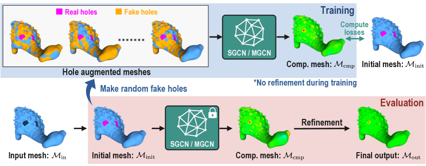
Figure 2: Overview of our self-supervised mesh inpainting. Our method, using only an input mesh with missing regions, consists of training and evaluation phases. In the training phase, the GCN is trained with meshes having different fake hole regions. The evaluation phase inputs the mesh with only real holes and outputs the hole-completed mesh. Refinement, performed only in the evaluation phase, is then applied to improve the vertex positions at both hole and non-hole regions.

3 Self-Supervised Mesh Inpainting by GCNs

Figure 2 shows the overview of our method, which consists of training and evaluation phases illustrated on the top and bottom, respectively. As explained later, our method solves the inpainting problem by moving the vertices of a smoothed input mesh to their correct positions. In other words, we “inpaint” the displacement vectors for the vertices rather than inpainting the positions of the vertices. Thus, we first fill the holes of the input mesh using a conventional hole-filling method.

During the training phase, we train a GCN using data augmentation, where several continuous regions on a single input mesh are marked as fake holes. We input a 4D vector into the GCN, with the first three entries representing a 3D vertex displacement and the last entry being either 0 or 1 to indicate if the corresponding vertex is masked by real/fake holes. If a vertex is masked, the 3D vertex displacement part is also filled with zeros. This enforces the GCN to treat displacement vectors at fake holes as unknown, just like those at real holes. In this manner, we train the GCN to predict displacement vectors in hole regions, allowing for self-supervised learning as we know the correct displacement vectors at fake holes.

During the evaluation phase, only the vertex displacements at real holes are estimated by the GCN without using fake holes. We restore the completed mesh by applying the displacements to the oversmoothed mesh. To further refine the precise shape of non-hole regions, we correct the vertex positions of both hole and non-hole regions by solving a least-squares problem [52].

Notations

We denote a mesh with the calligraphic symbol as $\mathcal{M}$, which may have boundaries and nonzero genus, and denote the sets of vertices and faces of $\mathcal{M}$ as $\mathcal{V}$ and $\mathcal{F}$, respectively. The positions of vertices and the normal vectors of faces are denoted as $\mathbf{X}\in\mathbb{R}^{|\mathcal{V}|\times 3}$ and $\mathbf{N}\in\mathbb{R}^{|\mathcal{F}|\times 3}$, respectively, where $|\mathcal{S}|$ is the size of the set $\mathcal{S}$. Additionally, we denote the $i$-th vertex position as $\mathbf{x}^{i}\in\mathbb{R}^{3}$ and the $j$-th facet normal as $\mathbf{n}^{j}\in\mathbb{S}^{2}$ (i.e., the set of unit vectors in $\mathbb{R}^{3}$). Thus, we denote the input mesh as $\mathcal{M}_{\rm in}$. We refer to intermediate output forms of the mesh by different names. The initial mesh $\mathcal{M}_{\rm init}$ refers to the mesh after preprocessing (see Section 3.1), which is input to the proposed networks described in Section 3.2. As we describe later, $\mathcal{M}_{\rm init}$ is a watertight mesh. Its surface is classified into the source region, which exists in the input mesh, and the target region, which is inserted by initial hole filling. We refer to the output mesh from the networks as a completed mesh, where the vertex positions at the target region are revised, and denote it as $\mathcal{M}_{\rm cmp}$. Finally, we revise the vertex positions of $\mathcal{M}_{\rm cmp}$ by the refinement step (see Section 3.5) to obtain the final output mesh $\mathcal{M}_{\rm out}$. We refer to the holes of the input mesh and those made during data augmentation (see Section 3.3) as “real” holes and “fake” holes, respectively. To identify vertices and normals in these hole regions, we introduce a mask $m_{\rm vtx}^{i}$ for the $i$-th vertex and $m_{\rm nrm}^{j}$ for the $j$-th facet normal, which take $0$ at hole regions and otherwise take $1$.

3.1 Input Mesh Preprocessing

The main difficulty of mesh inpainting is generating new vertices and faces in the missing regions. However, general GCNs, which we use in this paper, have difficulty inserting new vertices and triangles and changing the vertex connectivity. Therefore, instead of inserting new vertices and faces using the neural network, we first convert $\mathcal{M}_{\rm in}$ to a watertight manifold mesh using MeshFix [53], as shown in Fig. 3. Unfortunately, the densities between newly inserted vertices and originally existing vertices are inconsistent, which may worsen the performances of GCNs. To alleviate this problem, we obtain the initial mesh $\mathcal{M}_{\rm init}$ with uniform vertex density by applying triangular remeshing [54] after initial hole filling. After that, we train a neural network to learn the appropriate deformation of the initial mesh to obtain a complete mesh.

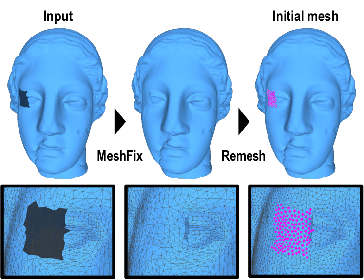
Figure 3: Generation of initial mesh $\mathcal{M}_{\rm init}$. We first obtain a watertight manifold mesh using MeshFix [53] (inserted vertices are colored pink) and then apply triangular remeshing [54] to achieve uniform vertex density.

In our inpainting, the network predicts the vertex displacements from the oversmoothed mesh rather than the vertex positions directly, which can encode more information about the local geometric features than the vertex positions. This idea was recently proposed by Hattori et al. [51] for mesh denoising, and they reported that it performed better when applying the DIP framework to mesh denoising. As shown in Fig. 4, vertices with similar geometric features are colored similarly when the mesh is colored based on the vertex displacement. To extract these local geometric features, we apply 30-step uniform Laplacian smoothing without cotangent weights for the initial oversmoothing.

The above preprocessing, i.e., triangular remeshing and oversmoothing, alleviates the artifacts caused by initial hole filling and makes our method independent of the initial hole filling algorithm. Instead of other hole-filling methods (e.g., the advancing front method [5] used in a later method [7] for the initial hole filling), we use MeshFix [53], which can always output a hole-filled mesh with the proper manifold structure.

3.2 Network Architectures

In this study, we consider two network architectures, SGCN and MGCN, to investigate the effect of network architecture on the mesh inpainting performance using a self-prior.

As its name indicates, SGCN performs the graph convolution defined on the mesh in the original resolution. SGCN consists of 13 graph convolution blocks and one vertex-wise fully connected layer. Each graph convolution block applies the Chebyshev spectral graph convolution (ChebConv) [55] followed by batch normalization and a leaky rectified linear unit (LeakyReLU).

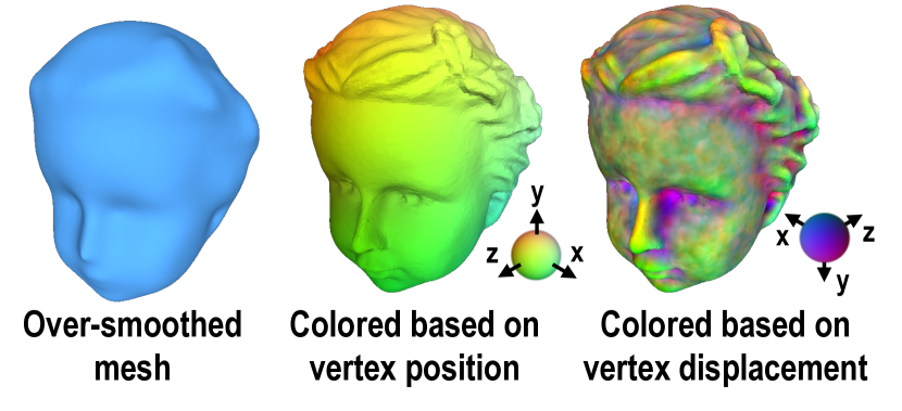
Figure 4: An oversmoothed mesh and meshes colored based on two geometric features. Local features are recognizable in the right mesh, colorized using vertex displacements, but not in the left. This shows that local features can be extracted by subtracting vertex positions of the oversmoothed mesh from those of the original. The two color spheres in the center and right are identical but viewed from opposite sides to present xthe colors for outward and inward displacements.

In contrast, MGCN employs an hourglass-type encoder-decoder network architecture. The encoder and decoder consist of several computation blocks. Each encoder block consists of five ChebConv layers with average mesh pooling, while each decoder block consists of five ChebConv layers with mesh unpooling. The last decoder block is followed by a single fully connected layer. The filter size of each ChebConv is determined by the order $K$ of the Chebyshev polynomial. We use $K=3$, corresponding to the convolution over vertices in 2-ring neighbors. Mesh pooling and unpooling are defined on a mesh using a precomputed static order of edge collapses, as described later. Due to space constraints, we provide additional details on the arrangement of these components in the supplementary document.

Mesh pooling and unpooling required for MGCN have not been extensively explored, and to our knowledge, there is still no standard approach. While dynamic mesh pooling and unpooling of MeshCNN [15] are good choices when computation time is not a concern, we found its memory and time efficiency inadequate for processing large meshes with tens or hundreds of thousands of triangles. Instead, we define pooling and unpooling operations on a mesh using a precomputed series of edge collapses. For mesh pooling, we collapse edges in ascending order of quadratic error metrics (QEMs) [56] until the number of vertices reaches the target. This process is similar to progressive meshes [28]. However, unlike the original approach, we add a penalty $P_{\rm val}$ to the QEM of the $i$-th vertex to prevent its valence $n_{\rm val}^{i}$ from being less than or equal to 3 after edge collapse, while also discouraging it from being more than 6.

$$P_{\rm val}=\begin{cases}\absolutevalue{n_{\rm val}^{i}-6}+1&(n_{\rm val}^{i}>3)\\ \infty&(\text{otherwise})\end{cases}$$ (1)

By introducing this penalty, we can obtain a simplified mesh with approximately regular triangulation without the edge flip and edge split. In this way, our mesh pooling and unpooling can be defined simply by only considering pairs of vertices consecutively merged by edge collapses.

During mesh simplification, we record which vertex is merged with another vertex. When a set of vertices is merged to the $i$-th vertex, the average mesh pooling is defined simply as

$$\mathbf{f}^{\prime}_{i}=\frac{1}{\absolutevalue{\mathcal{C}(i)}}\sum_{k\in\mathcal{C}(i)}\mathbf{f}_{k},$$ (2)

where $\mathbf{f}$ and $\mathbf{f}^{\prime}$ are the features before and after mesh pooling, respectively, and $\mathcal{C}(i)$ is an index set of the vertices merged to the $i$-th vertex. Conversely, the mesh unpooling simply assigns the feature $\mathbf{f}_{i}$ back to the merged vertices with the indices in $\mathcal{C}(i)$. In our experiment, we precompute meshes at $R=3$ different resolutions and define mesh pooling and unpooling between each pair of successive resolutions. To obtain a mesh with the next lower resolution, we reduce the number of vertices to $60\text{\,}\%$. The simplified meshes with intermediate resolutions are shown in Fig. 5.

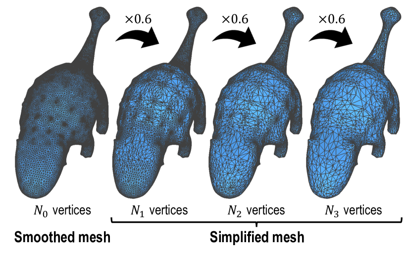
Figure 5: Meshes simplified using QEMs [56] defined on a smoothed mesh. Each simplification reduces the number of vertices to $60\text{\,}\%$, i.e., $N_{k}=\mathrm{round}(0.6N_{k-1})$.

3.3 Self-Supervision

Figure 6 illustrates the proposed self-supervised learning for mesh inpainting. As shown in this figure, the GCN transforms a feature vector assigned to each vertex to another vector. At the $i$-th vertex, the GCN transforms a 4D vector $(\Delta x_{\rm in}^{i},\Delta y_{\rm in}^{i},\Delta z_{\rm in}^{i},\hat{m}_{\rm vtx}^{i})$ to a 3D displacement vector $(\Delta x_{\rm out}^{i},\Delta y_{\rm out}^{i},\Delta z_{\rm out}^{i})$, where $\hat{m}_{\rm vtx}^{i}\in\{0,1\}$ represents whether the $i$-th vertex is masked by a hole ($\hat{m}_{\rm vtx}^{i}=0$) (i.e., either real or fake holes) or not ($\hat{m}_{\rm vtx}^{i}=1$).

However, there are two problems in training the GCN to predict such displacements. First, the displacements at hole regions are unknown, and we cannot assess the accuracy of the displacements estimated by the GCN. Second, since the input and output displacements of the vertices in non-hole regions are the same, training the GCNs is prone to become stuck in a trivial solution representing an identity mapping.

To solve these problems, we propose an approach to training the GCN in a self-supervised manner by introducing fake holes as well as real holes. At the vertices covered by either fake or real holes, we mask the input displacements by zero vectors, i.e., $(\Delta x_{\rm in}^{i},\Delta y_{\rm in}^{i},\Delta z_{\rm in}^{i})=(0,0,0)$, and set the mask as $\hat{m}_{\rm vtx}^{i}=0$. Then, the GCN is trained to predict the vertex displacements for the regions masked by real and fake holes based on the known displacements in the non-hole regions. Then, the output displacements from the GCN are added to the oversmoothed mesh to obtain the output completed mesh $\mathcal{M}_{\rm cmp}$. Because we know the correct displacement vectors at fake hole regions, we can penalize incorrect displacements using a loss function described later.

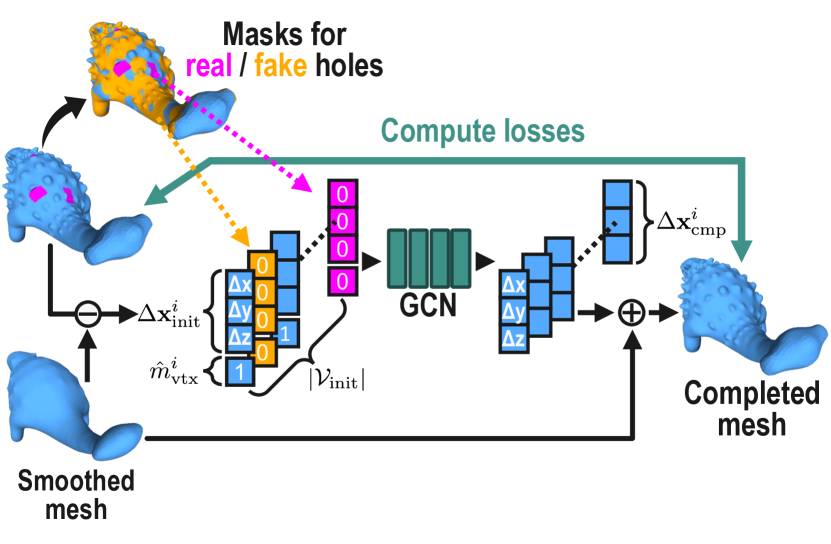
Figure 6: Self-supervision of the proposed GCN, where the GCN predicts the displacement of each vertex to reproduce the inpainted shape from the oversmoothed shape. We train the GCN in a self-supervised manner to predict the vertex displacements by filling zeros to the displacements at real and fake holes (colored pink and orange, respectively).

For self-supervision, we generate multiple sets of masks representing fake holes. Thus, we randomly select seed vertices with a certain probability $p$ and mark vertices inside the $k$-ring neighbor as included by fake holes. We set $p=$1.4\text{\,}\%$$ and $k=4$ such that approximately $60\text{\,}\%$ of the vertices are masked. During this data augmentation, we select 40 sets of random seed vertices, thus obtaining 40 different masks that represent fake holes.

3.4 Loss Functions

To train both SGCN and MGCN, we use three kinds of loss terms: the data term for vertex positions $E_{\rm pos}$, the data term for facet normals $E_{\rm nrm}$, and the smoothness term for the directions of facet normals $E_{\rm reg}$. In the following loss definitions, we simply denote the number of vertices and faces as $\absolutevalue{\mathcal{V}}$ and $\absolutevalue{\mathcal{F}}$, respectively, because $\absolutevalue{\mathcal{V}_{\rm init}}=\absolutevalue{\mathcal{V}_{\rm cmp}}$ and $\absolutevalue{\mathcal{F}_{\rm init}}=\absolutevalue{\mathcal{F}_{\rm cmp}}$.

Data term for vertex positions

The error for $\mathbf{X}_{\rm cmp}$, which is the output from the network, is calculated using the root mean squared error for the vertices that correspond to the original vertices of the input mesh $\mathcal{M}_{\rm in}$. Therefore, we define the data term for vertex positions by applying the mask $m_{\rm vtx}^{i}$ to exclude the vertices in the hole regions.

$$E_{\rm pos}({\mathbf{X}}_{\rm cmp},\!\mathbf{X}_{\rm init})\!=\!\quantity(\frac{1}{\sum_{i}m_{\rm vtx}^{i}}\sum_{i=1}^{\absolutevalue{\mathcal{V}}}m_{\rm vtx}^{i}\norm{{\mathbf{x}}_{\rm cmp}^{i}\!-\!\mathbf{x}_{\rm init}^{i}}_{2}^{2})^{\frac{1}{2}},$$ (3)

where $\norm{\,\cdot\,}_{p}$ is the $\ell_{p}$ norm of a vector. For multi-resolution meshes used by MGCN, the positional error $E_{\rm pos}^{(r)}$ is equivalently defined for each resolution level $r=0,1,\ldots$, and thus $E_{\rm pos}$ = $E_{\rm pos}^{(0)}$.

Data term for facet normals

Facet normal directions are an important factor in accurately reconstructing local geometric features, such as sharp edges. Our network outputs vertex positions $\mathbf{X}_{\rm cmp}$, from which we compute facet normals $\mathbf{N}_{\rm cmp}$ for each triangle. To ensure the facet normal directions of the network output match those of the input mesh’s original triangles, we define the data term for facet normals using mean absolute error for the existing triangles in $\mathcal{M}_{\rm in}$.

$$E_{\rm nrm}({\mathbf{N}}_{\rm cmp},\mathbf{N}_{\rm init})=\frac{1}{\sum_{j}m_{\rm nrm}^{j}}\sum_{j=1}^{\absolutevalue{\mathcal{F}}}m_{\rm nrm}^{j}\norm{\mathbf{n}_{\rm cmp}^{j}-\mathbf{n}_{\rm init}^{j}}_{1},$$ (4)

Unlike $E_{\rm pos}$, the data term $E_{\rm nrm}$ for facet normals is computed for only the mesh at the highest resolution (i.e., $r=0$) even for training MGCN because of the different aims of these loss terms. The purpose of $E_{\rm nrm}$ is to reproduce the sharp features of the input mesh, and thus, it does not work as we intend for meshes with lower resolutions where the sharp features of the original resolution may have vanished. Therefore, we compute $E_{\rm nrm}$ for the mesh with the finest resolution to save the computational cost.

Smoothness term for facet normals

As Mataev et al. [21] reported, the regularization term defined with denoised output can prevent the DIP’s neural network from overfitting to noise. In geometry processing, Hattori et al. [51] reported a similar fact that regularizing facet normals using bilateral normal filtering (BNF) [57] is effective in preserving sharp geometric features such as edges and corners. Following these studies, we introduce a regularizer as the smoothness term for facet normals.

$$E_{\rm reg}(\mathbf{N}_{\rm cmp})=\frac{1}{|\mathcal{F}|}\sum_{j=1}^{|\mathcal{F}|}\norm{\mathbf{n}_{\rm cmp}^{j}-S_{\rm bnf}^{(t)}(\mathbf{n}_{\rm cmp}^{j})}_{1},$$ (5)

where $S_{\mathrm{bnf}}^{(t)}$ denotes a smoothing function using BNF, and its superscript $t$ denotes that BNF is applied $t$ times. Our experiment shows that $t=5$ obtains good results for CAD models. As with $E_{\rm nrm}$, this smoothness term $E_{\rm reg}$ for the facet normals is only computed for the mesh with the finest resolution for the same reason explained in the previous paragraph. It is worth noting that $E_{\rm reg}$ is computed only for a CAD model to encourage the recovery of sharp edges and corners (i.e., $\lambda_{\rm reg}\neq 0$ only for CAD models as described in the next paragraph).

TABLE I: Weights for Loss Terms

Network	Type	$\lambda_{\rm pos}^{(0)}$	$\lambda_{\rm pos}^{(1)}$	$\lambda_{\rm pos}^{(2)}$	$\lambda_{\rm pos}^{(3)}$	$\lambda_{\rm nrm}$	$\lambda_{\rm reg}$
SGCN	CAD	$1.0$	—	—	—	4.0	$4.0$
	Non-CAD	$1.0$	—	—	—	1.0	$0.0$
	Real scan	$1.0$	—	—	—	1.0	$0.0$
MGCN	CAD	$0.35$	0.30	0.20	0.15	4.0	$4.0$
	Non-CAD	$0.35$	0.30	0.20	0.15	1.0	$0.0$
	Real scan	$0.35$	0.30	0.20	0.15	1.0	$0.0$

Total loss

Overall, we train the proposed networks using the following loss function.

$$E=\sum_{r=0}^{R}\lambda_{\rm pos}^{(r)}E_{\rm pos}^{(r)}+\lambda_{\rm nrm}E_{\rm nrm}+\lambda_{\rm reg}E_{\rm reg},$$ (6)

where $R$ is the number of mesh resolutions, i.e., $R=0$ for SGCN and $R=3$ for MGCN, and each $\lambda$ modulates the influence of the respective loss term. The weights we used in the following experiments are summarized in Table I. Note that the weights $\lambda_{\rm pos}^{(r)}$ for training MGCN are set as $\sum_{r}\lambda_{\rm pos}^{(r)}=1$ so that the positional error has an equivalent effect to that for SGCN.

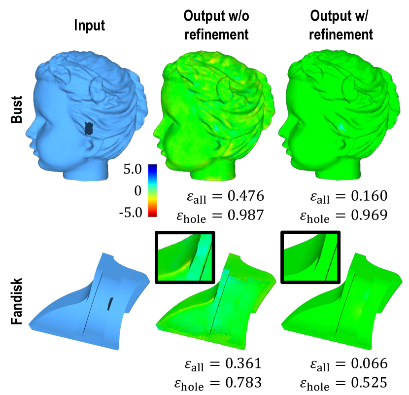
Figure 7: Effect of the refinement step for the outputs from MGCN. As this figure shows, the output shapes are significantly improved by the refinement step, as both _all and _hole (in the unit of $10^{-3}$) decrease significantly.

3.5 Refinement Step

As we mentioned previously, one of the problems of the DIP framework is the long processing time required to converge the optimization. We found that this problem is also common in polygonal meshes and optimizing network parameters requires considerable computation time to obtain $\mathbf{X}_{\rm cmp}$ which has equivalent vertex positions to those of $\mathbf{X}_{\rm init}$ in non-hole regions. To alleviate this problem, we introduce a refinement step to restore the vertex positions in non-hole regions rather than waiting for the optimization to converge. Note that the refinement is only performed in runtime and not in training.

For computational efficiency, we formulate this refinement step as a least-squares problem [52]. Let $\mathbf{L}=\mathbf{I}-\mathbf{D}^{-1}\mathbf{A}\in\mathbb{R}^{|\mathcal{V}|\times|\mathcal{V}|}$ be a Laplacian matrix of the mesh $\mathcal{M}_{\rm init}$ where $\mathbf{I}\in\mathbb{R}^{|\mathcal{V}|\times|\mathcal{V}|}$ is an identity matrix, $\mathbf{A}\in\mathbb{R}^{|\mathcal{V}|\times|\mathcal{V}|}$ is an adjacency matrix, and $\mathbf{D}\in\mathbb{R}^{|\mathcal{V}|\times|\mathcal{V}|}$ be a diagonal degree matrix. Specifically, we solve the following minimization problem to obtain the final output.

$$\mathbf{X}_{\rm out}=\operatorname*{argmin}_{\mathbf{X}}\frac{1}{2}\norm{\mathbf{L}\quantity(\mathbf{X}-\mathbf{X}_{\rm mix})}_{F}^{2}+\frac{\mu}{2}\norm{\mathbf{Q}\odot\quantity(\mathbf{X}-\mathbf{X}_{\rm init})}_{F}^{2},$$ (7)

where $\norm{\,\cdot\,}_{F}$ is the Frobenius norm of a matrix, and $\odot$ denotes a Hadamard product, i.e., an element-wise multiplication, of matrices. In this equation, $\mathbf{X}_{\rm mix}\in\mathbb{R}^{|\mathcal{V}|\times 3}$ is a matrix where its $i$-th row $\mathbf{x}_{\rm mix}^{i}$ is defined as

$$\mathbf{x}_{\rm mix}^{i}=\begin{cases}\mathbf{x}_{\rm init}^{i}&(m_{\rm vtx}^{i}=1),\\ \mathbf{x}_{\rm cmp}^{i}&(m_{\rm vtx}^{i}=0),\end{cases}$$ (8)

and the masking matrix $\mathbf{Q}\in\mathbb{R}^{|\mathcal{V}|\times 3}$ masks the vertices at hole regions and their boundaries, which is defined as

$$\mathbf{q}^{i}=\begin{cases}(0,0,0)&(i\in\bar{\mathcal{H}}),\\ (1,1,1)&(\mathrm{otherwise}),\end{cases}$$ (9)

where $\bar{\mathcal{H}}$ is a set of vertex indices that represents the union of hole regions $\mathcal{H}$ and its boundaries, i.e., the closure of $\mathcal{H}$.

$$\bar{\mathcal{H}}=\quantity{i:\exists j\in\{i\}\cup\mathcal{N}(i)\quad\mathrm{s.t.}\quad m_{\rm vtx}^{j}=0},$$ (10)

where $\mathcal{N}(i)$ is a set of indices for vertices next to the $i$-th vertex. We can solve the minimization in Eq. 7 as a sparse linear system and obtain the final refined output $\mathbf{X}_{\rm out}$.

Figure 7 shows the effect of the refinement. In this figure, _hole represents the average positional error over only the hole regions, whereas _all represents that over the entire mesh. Their formal definitions are described later in Section 4. As shown in the center of Fig. 7, the complete mesh inferred by the proposed GCN entails small positional deviations at non-hole regions. In contrast, the refinement step successfully reduces the deviations at both the hole and non-hole regions, as both _all and _hole decrease.

TABLE II: Quantitative Comparison of Inpainting Performance Using the Average Error Distance _hole in Units of $10^{-3}$

	Type	ADVF [5]	MFIX [53]	SPSR [58]	CCSC [7]	IPSR [59]	SGCN (ours)	MGCN (ours)
CG	CAD	13.900	$14.444$	11.141	10.641	13.453	3.376	$3.781$
Fandisk	CAD	5.692	$2.785$	3.346	4.944	4.945	1.890	$\BB 0.525$
Part-lp	CAD	9.464	$7.981$	6.524	8.476	8.431	1.543	$\BB 1.353$
Sharp-sphere	CAD	5.322	$5.412$	6.432	5.762	6.326	3.624	$3.853$
Ankylosaurus	Non-CAD	2.282	$3.334$	1.364	1.869	2.097	1.871	$\BB 1.317$
Bimba	Non-CAD	3.470	$2.813$	2.780	4.428	3.156	1.823	$2.397$
Bust	Non-CAD	1.572	$1.277$	1.421	2.070	1.642	0.942	$0.969$
Igea	Non-CAD	2.458	$2.114$	1.607	1.411	1.786	1.236	$1.779$
Bunny	Real scan	6.001	$5.551$	5.233	5.313	5.862	5.224	$5.299$
Dragon	Real scan	6.210	$3.232$	4.594	5.342	7.502	2.269	$2.565$

4 Experiments

Our method is implemented using PyTorch and PyTorch Geometric. It was tested on a computer equipped with Intel Core i7 5930K CPU ($3.5\text{\,}\mathrm{GHz}$, 6 cores), NVIDIA GeForce TITAN X GPU ($12\text{\,}\mathrm{G}\mathrm{B}$ graphics memory), and $64\text{\,}\mathrm{G}\mathrm{B}$ of RAM. We trained both SGCN and MGCN over 100 steps using the Adam optimizer with a learning rate of $\gamma=0.01$ and decay parameters $(\beta_{1},\beta_{2})=(0.9,0.999)$, where the learning rate is halved after 50 steps.

For intuitive understanding, we colorize the output meshes based on the signed distance between the output and ground truth meshes. For quantitative evaluation, we also calculate the average Euclidean distances between the vertices of the output and ground truth meshes in two manners: one for all vertices and the other for those inserted into the missing regions. These average distances are denoted as _all and _hole, respectively. The _all values are displayed only in Fig. 7 to show the effect of the refinement step, while the _hole values are shown in other figures and tables. These distances are normalized by the diagonal length of a bounding box of each mesh and are shown in units of $10^{-3}$.

We compared our results with those of previous methods, i.e., the advancing front method (ADVF) [5], MeshFix (MFIX) [53], screened Poisson surface reconstruction (SPSR) [58], context-based coherent surface completion (CCSC) [7], and iterative Poisson surface reconstruction (IPSR) [59], all of which do not use datasets and work only with an input mesh with holes. In this comparison, we used 13 meshes, including CAD, non-CAD, and real-scanned models. The quantitative evaluations were conducted only for 10 meshes with known ground truth geometries and are summarized in Table II.

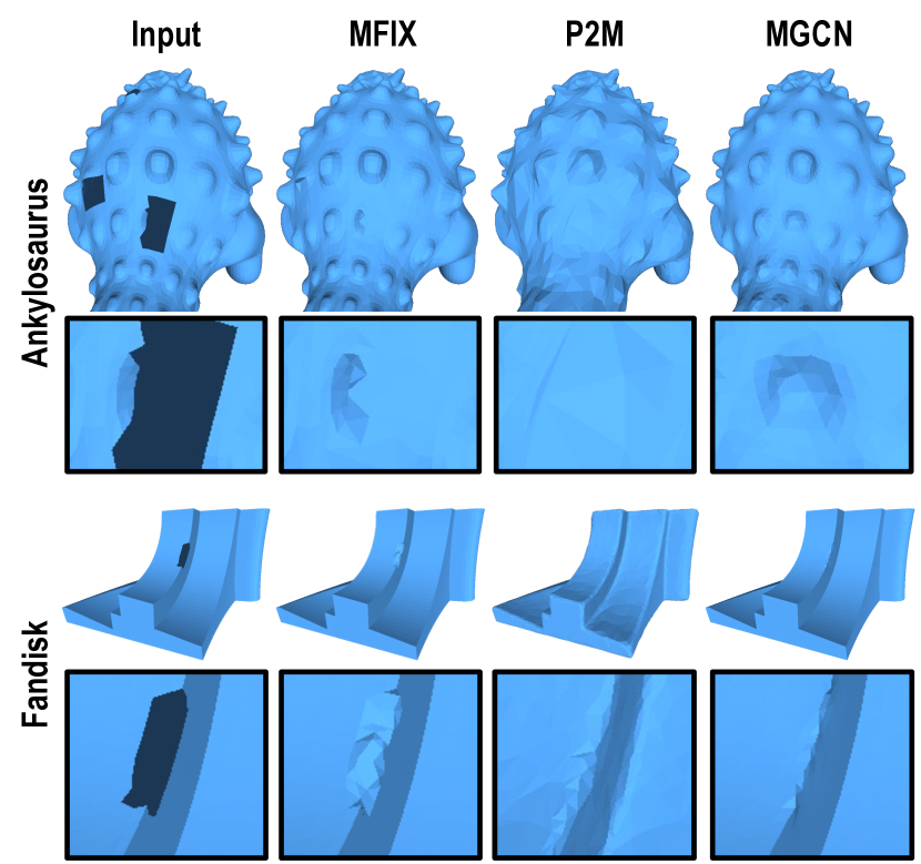
Figure 8: Comparison of results between MeshFix (i.e., our baseline), our method, and Point2Mesh [24].

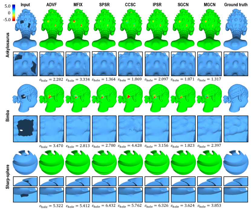
Figure 9: Visual comparison of inpainting performance for meshes with artificial holes. The output meshes are colored based on the distance to the ground truth, and the average distance from the output mesh at holes _hole is displayed below each mesh. Note that the positional error for MeshFix is computed after the hole-filled regions are remeshed.

In addition to the traditional approaches above, we compared the result from MGCN and that from Point2Mesh (P2M) [24], a self-supervised surface reconstruction method similar to ours. As Fig. 8 shows, P2M appears capable of capturing the self-similarity of the input geometry. However, in our testing environment, P2M was only applicable to low-resolution meshes because MeshCNN [15], its backend network, requires a large amount of graphics memory. In contrast, our method employs memory-efficient GCNs as a backend and has successfully restored characteristic shape features (e.g., repetitive bumps on the ankylosaurus’ back) and sharp edges (e.g., those of fandisk) while maintaining mesh resolution.

Although we also compared our method with recent data-driven methods for shape completion (i.e., PMP-Net [41], IF-Net [42], and ShapeFormer [45]), we found that their results are strongly affected by shapes in the training datasets. Therefore, the main body of the paper in the following only shows the comparison of the proposed methods with traditional methods that do not use datasets. Refer to the supplementary document for the comparison with the data-driven methods.

4.1 Results on CAD and Non-CAD Models

The top eight rows of Table II show the quantitative analysis for the CAD and non-CAD models. As these models do not originally have holes, we make several “artificial” holes and consider them as real holes. The visual comparisons for some of these models are also shown in Fig. 9. As this figure shows, traditional methods, such as ADVF [5] and MFIX [53], are prone to inpaint holes with a planar shape because they are based solely on local geometry processing. SPSR [58] and IPSR [59], the variants of Poisson surface reconstruction [60], often inpaint holes with oversmoothed patches and fail to recover sharp features, such as edges, and corners. In contrast to these methods, CCSC [7] may be able to recover the characteristic object shapes. However, we tested CCSC with several meshes and found that its results did not always match the shapes around holes. Additionally, the quantitative evaluation for CCSC was not as good as that of other methods (see Table II), although CCSC could insert the patches more complicated than the previous methods. In contrast to these previous methods, our method successfully restores missing details and sharp features, and either SGCN or MGCN achieved the lowest _hole for all the meshes.

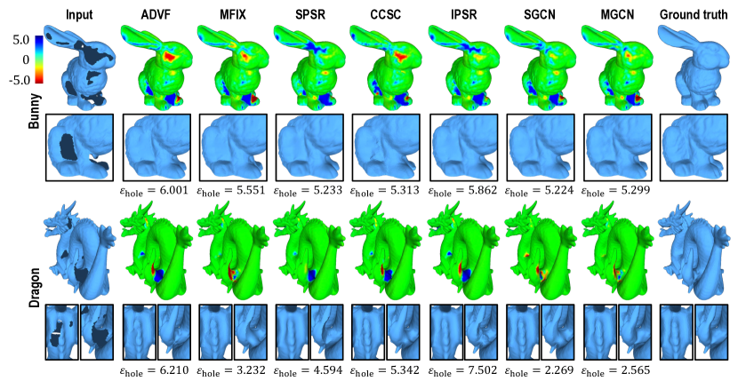
Figure 10: Visual comparison of inpainting performance for real scans provided by the Stanford 3D Repository [61].

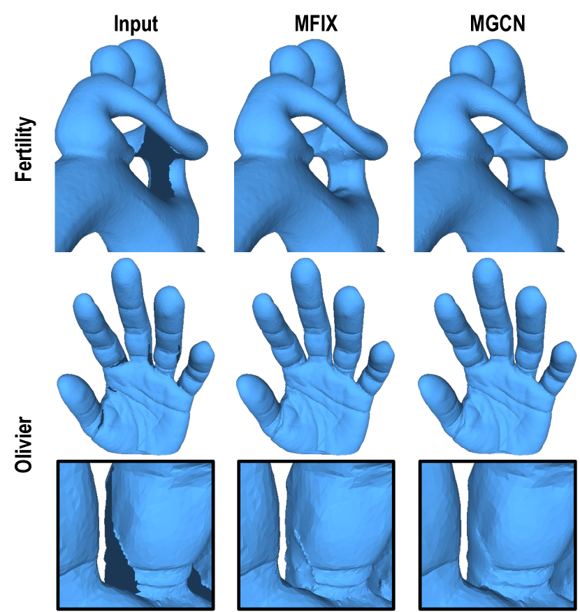
Figure 11: Inpainting results for real scans distributed by the AIM@SHAPE Shape Repository [62].

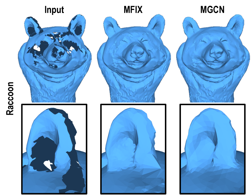
Figure 12: Inpainting results for a real scan obtained by an optical 3D scanner (GOM ATOS Core 135).

4.2 Results on Real-Scanned Models

Firstly, we evaluated our method using real-scanned models provided by the Stanford 3D Repository [61], where incomplete range scans are provided for each model. Using a set of range scans of each model, we synthesized an input mesh with missing regions by excluding some of the range scans and synthesized its corresponding complete mesh using all the range scans. Specifically, we excluded 6/10 and 15/45 range scans to obtain bunny and dragon models, respectively, with missing regions. Since the range scans are provided as point clouds, we obtained the surface geometries of incomplete and complete meshes using SPSR [58]. Although SPSR may fill the missing regions of an incomplete point cloud, we identified the missing regions by thresholding the triangle sizes.

Figure 10 shows the visual comparison with the models from the Stanford 3D Repository, which shows that these real-scanned models contain large holes with complicated shapes. In particular, a large hole between the bunny’s front legs cannot be inpainted by all the methods, while SGCN achieves among the lowest _hole. In contrast, for the dragon model, both our SGCN and MGCN achieve far lower _hole than all the other methods, more naturally reproducing the characteristic shapes of the crest on the dragon’s back and the scaly skin on the dragon’s body.

Secondly, we examined the performance of our method with a more practical scenario and compared the results with MFIX [53] as a baseline, which we used for the initial hole filling. Figure 11 shows the results for the real scans provided by the AIM@SHAPE Shape Repository [62]. For the fertility model, we generated the incomplete input mesh as performed with the models in the Stanford 3D Repository. For the Olivier model, we directly applied our method to the provided mesh that originally had missing regions at occluded parts between fingers. As Fig. 11 shows, MFIX fills the holes well in terms that the approximate shape is reproduced, while our method appropriately moves the vertices to reproduce the object shapes more naturally.

Figure 12 shows the results for the real-scanned model of a plastic raccoon toy, which we obtained using an optical 3D scanner (GOM ATOS Core 135). Because of the self-occlusion at the ears and the black color around the eyes, this model has many complicated holes. As with the previous results, while MFIX plausibly fills the holes, the result of our method is visually more natural, particularly at the ear enlarged in Fig. 12 and the regions around the right eye and cheek (i.e., the left side of the raccoon’s face).

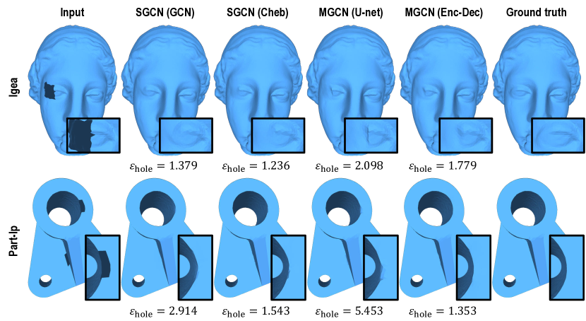
Figure 13: Comparison of output meshes obtained with different network architectures.

TABLE III: Inpainting Performance Comparison Across Different Network Architectures

	MFIX	SGCN
	SGCN	(GCN)
	MGCN
	MGCN
	(Enc-Dec)
Ankylo.	3.334	$1.875$	1.871	2.492	1.317
Igea	2.114	$1.379$	1.236	2.098	1.779
Fandisk	2.785	$1.377$	1.890	3.527	0.525
Part-lp	7.981	$2.914$	1.543	5.453	1.353
∗The values in this table are hole in units of $10^{-3}$

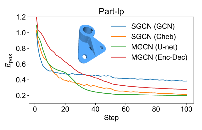
Figure 14: Comparison of the speed of $E_{\rm pos}$ convergence across different network architectures.

4.3 Comparison of Different Network Architectures

We now investigate other possible structures of SGCN and MGCN. While we constructed both SGCN and MGCN using ChebConv [55] as a graph convolution layer, we may also be able to employ GCNConv, the more efficient graph convolution, proposed by Kipf and Welling [63], which is widely known as a standard graph convolution layer. GCNConv is regarded as an approximation of ChebConv with a Chebyshev polynomial of order $K=2$ and is expected to perform similarly. Furthermore, since MGCN employs an hourglass-type encoder-decoder structure, we may also introduce skip connections to make it resemble U-net [64] and multi-resolution CNN [65], which have proven effective in deep feature extraction for various applications.

Figures 13 and III show the visual and quantitative comparisons of the structures using these options. In comparing the two types of SGCN, one with GCNConv (i.e., SGCN (GCN)) and the other with ChebConv (i.e., SGCN (Cheb)), their performance is found to be equivalent. However, we observed an interesting behavior that the training process, specifically the network parameter optimization, was more stable when using ChebConv rather than GCNConv. This behavior is evident in Table III, where _hole values are consistently low for various inputs. Moreover, the instability problem of GCNConv becomes more serious when used with MGCN. In particular, the training process of MGCN with GCNConv did not converge to any meaningful solutions. Thus, we excluded the results of ”MGCN (GCN)” from Figs. 13 and III.

TABLE IV: Comparison of Running Times for Loss Convergence Across Different Network Architectures

			Time
			SGCN (GCN) 300 steps	SGCN (Cheb) 100 steps	MGCN (Enc-Dec) 100 steps
	Vertices	Faces
Ankylo.	21090	42176	$42^{\prime}~{}21^{\prime\prime}$	28’ 43”	24’ 21”
Igea	44143	88282	$93^{\prime}~{}16^{\prime\prime}$	61’ 56”	48’ 56”
Fandisk	16724	33444	$37^{\prime}~{}47^{\prime\prime}$	24’ 17”	19’ 42”
Part-lp	10165	20338	$22^{\prime}~{}09^{\prime\prime}$	14’ 13”	13’ 29”

The effect of skip connections to MGCN can be observed in Table III, which shows that “MGCN (Enc-Dec),” a simple encoder-decoder architecture without skip connections, outperforms “MGCN (U-net),” which incorporates skip connections, similar to the U-net architecture. Such a behavior is also reported in the original DIP paper [20]. Our result suggests that skip connections are detrimental when applying the DIP framework also to polygonal meshes.

When it comes to the relationship between convergence speed and output quality, a network architecture exhibiting faster training convergence is found to obtain better results. For example, Fig. 14 shows that training of “SGCN (Cheb)” converges faster than that of “SGCN (GCN),” and the former obtains better results as described above. However, as we discussed previously, skip connections do not improve the inpainting performance despite the faster convergence of “MGCN (U-net)” than “MGCN (Enc-Dec).” During our experiment, we observed that networks with skip connections are prone to becoming stuck in a trivial solution representing an identity mapping. Based on these observations, we speculate that this issue may arise from the difference in inductive bias introduced by the networks with and without skip connections.

Table IV compares the computation times for different models needed to iterate the optimization over 100 steps, which shows that “SGCN (Cheb)” and “MGCN (Enc-Dec)” work almost equally in time. As shown in Fig. 14, the network with GCNConv converges more slowly, but the time required for forward and backward network evaluations is shorter than that with ChebConv. However, when SGCN utilizes GCNConv, it requires three times the number of steps (i.e., 300 steps) to achieve a loss value as small as the one attained by SGCN that employs ChebConv. As a result, the total time required to achieve the same loss value is longer with GCNConv, as we showed in Table IV. Thus, ChebConv is a preferable choice for graph convolution, also in terms of time performance. It should be noted that incorporating skip connections into MGCN had a negligible effect on the computation time.

Currently, the time required by our method remains longer than that of other traditional approaches, as other self-prior-based methods, because these techniques have still been evolving. For instance, even CCSC [7], one of the traditional methods known for its comparatively longer processing time, typically takes no more than ten minutes for an input mesh with several tens of thousands of triangles (e.g., it took about 7 minutes for the Igea model with approximately 90000 triangles). In contrast, our method exhibits a significant speed advantage over P2M [24], a recent self-prior-based approach, required approximately two hours in our testing environment, even for an input mesh with approximately ten thousand triangles.

4.4 Effect of Error Terms

TABLE V: Ablation Study for MGCN’s Losses

	MFIX	MGCN	MGCN
	MGCN		w/o $E_{\rm pos}^{(1,2,3)}$
	MGCN
	w/o $E_{\rm nrm}$
$E_{\rm pos}^{(0)}$	—	✓	$\checkmark$	✓	✓
$E_{\rm pos}^{(1,2,3)}$	—	✓	×	✓	✓
$E_{\rm nrm}$	—	✓	$\checkmark$	✓	$\times$
$E_{\rm reg}$	—	✓	$\checkmark$	$\times$	$\times$
Ankylo.	3.334	1.317	$1.533$	—	1.619
Igea	2.114	1.779	$1.949$	—	1.952
Fandisk	2.785	0.525	$0.717$	0.568	2.289
Part-lp	8.035	1.353	$1.501$	2.165	7.299
∗The values in this table are hole in units of $10^{-3}$

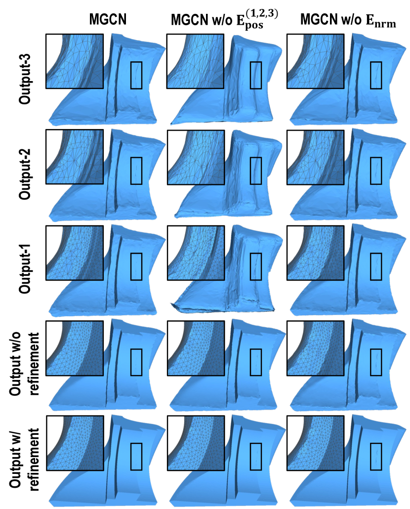
Figure 15: Comparison of output meshes at different resolutions. While the outputs after the refinement step appear nearly identical, there are subtle differences in the shapes of areas that were initially holes (best viewed on screen).

Section 4.4 shows the _hole values obtained by an ablation study on error terms used to train MGCN. In this table, ablated losses for each MGCN variant are marked by a cross mark “$\times$”, while remaining losses are marked by a check mark “✓”. It should be noted that the label, “w/o $E_{\rm nrm}$,” denotes the corresponding MGCN variant does not consider normal vectors at all and does not employ either $E_{\rm nrm}$ or $E_{\rm reg}$, as shown in Section 4.4. Along with this table, Fig. 15 shows the visual analyses on the output meshes with different resolutions. In Sections 4.4 and 15, we excluded either the sum of a part of multi-resolution reconstruction terms, i.e., $E_{\rm pos}^{(1,2,3)}\triangleq\sum_{r=1}^{3}E_{\rm pos}^{(r)}$, normal reconstruction term $E_{\rm nrm}$, or regularization term $E_{\rm reg}$. Since $E_{\rm reg}$ is not used for non-CAD models, i.e., ankylosaurus and Igea models, horizontal lines are drawn in the respective cells.

As Fig. 15 shows, excluding $E_{\rm pos}^{(1,2,3)}$ causes the network to neglect the intermediate low-resolution output meshes, and as a result, the reproduction of the vertex positions at the original resolution is spoiled, as shown in Section 4.4. Moreover, when $E_{\rm nrm}$ is excluded, the reproduction of sharp features, such as edges and corners, at hole regions is limited, although those at non-hole regions can be reproduced properly by the refinement step, as shown in Fig. 15. Thus, the result also worsens quantitatively, as shown in Section 4.4. In addition, Section 4.4 shows that _hole deteriorates by ablating the regularizer, which suggests that the facet normal regularizer $E_{\rm reg}$ is important for reproducing the sharp features. Thus, all the error terms used to train MGCN are essential to maximizing the performance of the proposed method.

TABLE VI: Effect of Fake Hole Size

	$k=2$	$k=4$	$k=6$
Ankylosaurus	1.689	1.317	$1.393$
Igea	1.946	1.779	$\BB 1.677$
Fandisk	0.487	0.525	$0.719$
Part-lp	1.220	1.353	$2.685$
∗The values in this table are hole in units of $10^{-3}$

TABLE VII: Effect of Probability of Fake Hole Occurrence

	$p=$0.7\text{\,}\%$$	$p=$1.4\text{\,}\%$$	$p=$2.1\text{\,}\%$$
Ankylosaurus	1.358	1.317	$1.318$
Igea	2.020	1.779	$\BB 1.761$
Fandisk	0.900	0.525	$1.173$
Part-lp	1.685	1.353	$4.961$
∗The values in this table are hole by the unit of $10^{-3}$

4.5 Effect of Fake Hole Size and Occurrence

Table VII compares _hole values obtained by MGCN trained using different mask sizes. When we select seed vertices with a fixed probability $p=$1.4\text{\,}\%$$, the mask sizes $k=2$, $4$, and $6$ mark approximately $25\text{\,}\%$, $60\text{\,}\%$, and $85\text{\,}\%$ vertices, respectively, as covered by fake holes. While the optimal mask size for each mesh varies, this table suggests that a relatively small mask size (i.e., $k=2,4$) performs better. A large mask size (e.g., $k=6$) may diminish the performance.

Similar behavior can be observed when varying the probability of selecting seed vertices. Table VII compares _hole values obtained by MGCN trained with different seed occurrence probabilities. When we fix the mask size as $k=4$, the probabilities $p=$0.7\text{\,}\%$$, $1.4\text{\,}\%$, and $2.1\text{\,}\%$ mark approximately $35\text{\,}\%$, $60\text{\,}\%$, and $75\text{\,}\%$ vertices, respectively, as covered by fake holes. As with varying mask sizes, smaller probabilities of seed vertex occurrence often obtain better scores, while a larger probability $p=$2.1\text{\,}\%$$ may result in worse scores than that of the smaller probabilities.

Moreover, training the network using fewer sets of mask patterns is prone to slow down the convergence. On the other hand, using a large number of mask patterns requires much more time to train the network over the same number of epochs. As a result, we concluded that 40 different mask patterns were the best to balance the computational efficiency and the inpainting quality.

4.6 Limitations

Although our method works well for most incomplete meshes we tested, it has several limitations. Currently, our method works when the expected complete shape for an input mesh is watertight. Unfortunately, isolated elements are lost in our current implementation due to the limitations of MeshFix. Furthermore, as with previous methods that do not use large-scale datasets, characteristic shapes that cannot be observed in the non-hole regions cannot be recovered even with our method. Finally, our method requires several minutes of training for each input, although its computation time is shorter than that of other self-supervised methods.

5 Conclusion

In this study, we investigated GCNs that acquire a self-prior for mesh inpainting by self-supervised learning. As our method leverages the self-prior, it does not require heuristics, user interaction, or large-scale training datasets. Furthermore, our method works on meshes without converting them to other shape formats, such as point clouds, voxel grids, and implicit functions. In this sense, our method can be used as traditional approaches that are not based on machine learning and can achieve better shape qualities on inpainted meshes than such traditional approaches.

In future work, we are interested in extending our method using more advanced DIP variants (e.g., [21, 22, 23]). Utilizing these sophisticated approaches may reduce the necessary sets of mask patterns for our self-supervised mesh inpainting, further decreasing computation time. Additionally, we are interested in leveraging vertex colors alongside vertex positions, as most off-the-shelf 3D scanners capture both. Lastly, although recent studies [66, 67, 68] have proposed potential ideas, improving the time and memory efficiency of basic neural network layers (e.g., convolution and dynamic pooling/unpooling) for meshes remains an important and challenging research direction.

Acknowledgments

We would like to thank the Stanford 3D Repository and AIM@SHAPE Shape Repository for providing the 3D models. Tatsuya Yatagawa is supported by the JSPS Grant-in-Aid for Early-Career Scientists (22K17907).

Shota Hattori, Tatsuya Yatagawa, Yutaka Ohtake, and Hiromasa Suzuki

A MGCN Architecture

Architecture

The multi-resolution graph convolutional network (MGCN) has an encoder-decoder architecture, but unlike the U-net architecture, skip connections are not incorporated. Figure A1 illustrates the MGCN architecture. As discussed in the main text, the pooling and unpooling operations that are required to define the encoder-decoder network are defined using multi-resolution meshes computed in advance by the technique, progressive meshes [28].

Input and output

As depicted in the figure, the input to MGCN consists of a graph structure defined by vertex connections on the input mesh, and a set of feature vectors, each assigned to a vertex. Each 4D feature vector, mentioned earlier in the main text, is transformed by the network into a 3D vector representing the displacement needed to reproduce the completed mesh from the smoothed version of the initial mesh.

Multi-resolution supervision

As demonstrated in the ablation study in Section 4.4, achieving high-quality mesh inpainting requires multi-resolution supervision for vertex positions. This supervision is performed by forwarding the intermediate output from each UpConv block to a separate graph convolution layer (denoted as “Conv” in Fig. A1 and depicted by a purple arrow), which produces vertex displacements for the lower-resolution version of the initial mesh.

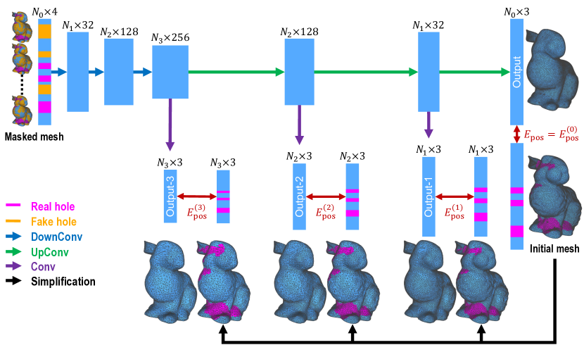
Figure A1: The illustration of the MGCN architecture.

B Input meshes and hyperparameters

Figure B2 shows all the meshes with missing regions used in our experiments, and Table B1 shows the information on each mesh, i.e., the type (i.e., either of “Non-CAD”, “CAD”, or “Real scan”), the number of vertices and triangles, and the weight parameter $\mu$ used in the refinement step.

As for the types of meshes, the non-CAD and CAD models are the models where only an entire shape of each mesh is provided in the shape repository. We classified the models into either non-CAD or CAD ones based on whether sharp geometric features, such as edges and corners, are distinctive in each shape or not. Therefore, the names of the types, i.e., non-CAD and CAD, do not mean whether they are made by CAD software or not. In contrast, real-scan models shown here are prepared using only some of the range scans provided in the shape repositories [61, 62].

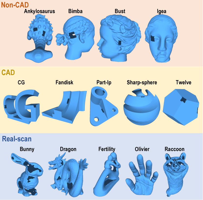
Figure B2: All the meshes used in our experiments.

TABLE B1: Details of Meshes Used in Our Experiments

	Type	Vertices	Faces	$\mu$
Ankylosaurus	Non-CAD	$21090$	42176	1.0
Bimba	Non-CAD	$24132$	48260	1.0
Bust	Non-CAD	$33967$	67930	1.0
Igea	Non-CAD	$44143$	88282	1.0
CG	CAD	$9949$	19894	0.1
Fandisk	CAD	$16724$	33444	0.01
Part-lp	CAD	$10165$	20338	0.01
Sharp-sphere	CAD	$18084$	36164	0.1
Twelve	CAD	$11362$	22720	0.1
Bunny	Real scan	$30272$	60540	1.0
Dragon	Real scan	$35248$	70496	1.0
Fertility	Real scan	$29907$	59826	1.0
Olivier	Real scan	$29509$	59014	1.0
Raccoon	Real scan	$30318$	60632	1.0

C Comparison with data-driven methods

In contrast to our method, which operates on an incomplete input mesh, many previous studies are based on fully-supervised deep learning. To examine the performance of such approaches on the input meshes used in our experiment, we compared our results with those of three data-driven methods: PMP-Net [41], IF-Net [42], and ShapeFormer [45]. PMP-Net operates on point clouds, while the other two work on surface geometries using implicit functions as an intermediate format.

Figure C3 presents the comparison results. In this experiment, we utilized the code and predefined weights provided by the authors of PMP-Net^1., IF-Net^2., and ShapeFormer^3.. As depicted in Fig. C3, all these methods, unfortunately, failed to inpaint the shape geometries since these inputs (ankylosaurus and sharp sphere models in this figure) are not included in the datasets used by these data-driven methods. In contrast, our method is independent of training datasets. Nonetheless, it can effectively inpaint arbitrary shapes, resulting in natural-looking inpainted geometries.

On the other hand, data-driven methods have advantages in runtime speed. As long as a given shape that a user wants to inpaint resembles some shapes in the dataset, these methods can achieve both high quality and speed. Therefore, there is a trade-off between data-driven methods and self-prior-based approaches like our method.

1. PMP-Net: https://github.com/diviswen/PMP-Net, accessed on Apr. 5th, 2023

2. IF-Net: https://github.com/jchibane/if-net, accessed on Apr. 5th, 2023

3. ShapeFormer https://github.com/qheldiv/shapeformer, accessed on Apr. 5th, 2023

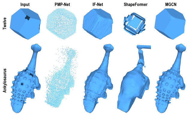
Figure C3: Comparison with recent data-driven methods, i.e., PMP-Net [41], IF-Net [42], and ShapeFormer [45].

References

- [1] G. Barequet and M. Sharir, “Filling gaps in the boundary of a polyhedron,” Computer Aided Geometric Design, vol. 12, no. 2, pp. 207–229, 1995.
- [2] P. Liepa, “Filling holes in meshes,” in Proceedings of Eurographics Symposium on Geometry Processing (SGP), vol. 30, 2003, pp. 200–206.
- [3] U. Clarenz, U. Diewald, G. Dziuk, M. Rumpf, and R. Rusu, “A finite element method for surface restoration with smooth boundary conditions,” Computer Aided Geometric Design, vol. 21, no. 5, pp. 427–445, 2004.
- [4] J.-P. Pernot, G. Moraru, and P. Véron, “Filling holes in meshes using a mechanical model to simulate the curvature variation minimization,” Computers & Graphics, vol. 30, no. 6, pp. 892–902, 2006.
- [5] W. Zhao, S. Gao, and H. Lin, “A robust hole-filling algorithm for triangular mesh,” in Proceedings of the 10th IEEE International Conference on Computer-Aided Design and Computer Graphics, 2007, pp. 22–22.
- [6] A. Sharf, M. Alexa, and D. Cohen-Or, “Context-based surface completion,” ACM Transactions on Graphics, vol. 23, no. 3, pp. 878–887, 2004.
- [7] G. Harary, A. Tal, and E. Grinspun, “Context-based coherent surface completion,” ACM Transactions on Graphics, vol. 33, no. 1, 2014.
- [8] J. Jam, C. Kendrick, K. Walker, V. Drouard, J. G.-S. Hsu, and M. H. Yap, “A comprehensive review of past and present image inpainting methods,” Computer Vision and Image Understanding, vol. 203, p. 103147, 2021.
- [9] H. Xiang, Q. Zou, M. A. Nawaz, X. Huang, F. Zhang, and H. Yu, “Deep learning for image inpainting: A survey,” Pattern Recognition, vol. 134, 2023.
- [10] Z. Wu, S. Song, A. Khosla, F. Yu, L. Zhang, X. Tang, and J. Xiao, “3D ShapeNets: A deep representation for volumetric shapes,” in Proceedings of the IEEE Conference on Computer Vision and Pattern Recognition, 2015, pp. 1912–1920.
- [11] A. Dai, C. R. Qi, and M. NieBner, “Shape completion using 3D-encoder-predictor CNNs and shape synthesis,” in Proceedings of the IEEE Conference on Computer Vision and Pattern Recognition, 2017, pp. 6545–6554.
- [12] W. Yuan, T. Khot, D. Held, C. Mertz, and M. Hebert, “Pcn: Point completion network,” in Proceedings of IEEE International Conference on 3D Vision, 2018, pp. 728–737.
- [13] X. Wen, T. Li, Z. Han, and Y.-S. Liu, “Point cloud completion by skip-attention network with hierarchical folding,” in Proceedings of the IEEE/CVF Conference on Computer Vision and Pattern Recognition, 2020, pp. 1939–1948.
- [14] Y. Feng, Y. Feng, H. You, X. Zhao, and Y. Gao, “MeshNet: Mesh neural network for 3D shape representation,” in Proceedings of the AAAI Conference on Artificial Intelligence, vol. 33, no. 01, 2019, pp. 8279–8286.
- [15] R. Hanocka, A. Hertz, N. Fish, R. Giryes, S. Fleishman, and D. Cohen-Or, “MeshCNN: A network with an edge,” ACM Transactions on Graphics, vol. 38, no. 4, 2019.
- [16] M.-J. Rakotosaona, N. Aigerman, N. J. Mitra, M. Ovsjanikov, and P. Guerrero, “Differentiable surface triangulation,” ACM Transactions on Graphics, vol. 40, no. 6, pp. 1–13, 2021.
- [17] N. Sharp, S. Attaiki, K. Crane, and M. Ovsjanikov, “DiffusionNet: Discretization agnostic learning on surfaces,” ACM Transactions on Graphics, vol. 41, no. 3, pp. 1–16, 2022.
- [18] Q. Zhou and A. Jacobson, “Thingi10K: A dataset of 10,000 3D-printing models,” arXiv preprint arXiv:1605.04797, 2016.
- [19] S. Koch, A. Matveev, Z. Jiang, F. Williams, A. Artemov, E. Burnaev, M. Alexa, D. Zorin, and D. Panozzo, “Abc: A big cad model dataset for geometric deep learning,” in Proceedings of the IEEE/CVF Conference on Computer Vision and Pattern Recognition, 2019.
- [20] D. Ulyanov, A. Vedaldi, and V. Lempitsky, “Deep image prior,” in Proceedings of the IEEE Conference on Computer Vision and Pattern Recognition, 2018, pp. 9446–9454.
- [21] G. Mataev, P. Milanfar, and M. Elad, “DeepRED: Deep image prior powered by red,” in Proceedings of the IEEE/CVF International Conference on Computer Vision Workshops, 2019, pp. 0–0.
- [22] Z. Cheng, M. Gadelha, S. Maji, and D. Sheldon, “A bayesian perspective on the deep image prior,” in Proceedings of the IEEE/CVF Conference on Computer Vision and Pattern Recognition, 2019, pp. 5443–5451.
- [23] Y. Jo, S. Y. Chun, and J. Choi, “Rethinking deep image prior for denoising,” in Proceedings of the IEEE/CVF International Conference on Computer Vision, 2021, pp. 5087–5096.
- [24] R. Hanocka, G. Metzer, R. Giryes, and D. Cohen-Or, “Point2mesh: A self-prior for deformable meshes,” ACM Transactions on Graphics, vol. 39, no. 4, 2020.
- [25] X. Wei, Z. Chen, Y. Fu, Z. Cui, and Y. Zhang, “Deep hybrid self-prior for full 3D mesh generation,” in Proceedings of the IEEE/CVF International Conference on Computer Vision, 2021.
- [26] L. Chu, H. Pan, and W. Wang, “Unsupervised shape completion via deep prior in the neural tangent kernel perspective,” ACM Transactions on Graphics, vol. 40, no. 3, pp. 1–17, 2021.
- [27] H. Mittal, B. Okorn, A. Jangid, and D. Held, “Self-supervised point cloud completion via inpainting,” in Proceedings of British Machine Vision Conference (BMVC), 2021.
- [28] H. Hoppe, “Progressive meshes,” in Proceedings of ACM International Conference on Computer Graphics and Interactive Techniques, 1996, pp. 99–108.
- [29] V. Kraevoy and A. Sheffer, “Template-based mesh completion,” in Proceedings of Eurographics Symposium on Geometry Processing (SGP), M. Desbrun and H. Pottmann, Eds., 2005.
- [30] J. Davis, S. R. Marschner, M. Garr, and M. Levoy, “Filling holes in complex surfaces using volumetric diffusion,” in Proceedings of the 1st International Symposium on 3D Data Processing Visualization and Transmission, 2002, pp. 428–441.
- [31] J. Verdera, V. Caselles, M. Bertalmio, and G. Sapiro, “Inpainting surface holes,” in Proceedings the International Conference on Image Processing (ICIP), vol. 2, 2003.
- [32] T.-Q. Guo, J.-J. Li, J.-G. Weng, and Y.-T. Zhuang, “Filling holes in complex surfaces using oriented voxel diffusion,” in Proceedings of the International Conference on Machine Learning and Cybernetics, 2006, pp. 4370–4375.
- [33] S. Bischoff, D. Pavic, and L. Kobbelt, “Automatic restoration of polygon models,” ACM Transactions on Graphics, vol. 24, no. 4, pp. 1332–1352, 2005.
- [34] Y. LeCun and Y. Bengio, Convolutional Networks for Images, Speech, and Time Series. Cambridge, MA, USA: MIT Press, 1998, pp. 255–258.
- [35] C. R. Qi, H. Su, K. Mo, and L. J. Guibas, “PointNet: Deep learning on point sets for 3D classification and segmentation,” in Proceedings of the IEEE Conference on Computer Vision and Pattern Recognition, 2017, pp. 652–660.
- [36] C. R. Qi, L. Yi, H. Su, and L. J. Guibas, “PointNet++: Deep hierarchical feature learning on point sets in a metric space,” in Advances in Neural Information Processing Systems, 2017.
- [37] J. Varley, C. DeChant, A. Richardson, J. Ruales, and P. Allen, “Shape completion enabled robotic grasping,” in Proceedings of the IEEE/RSJ International Conference on Intelligent Robots and Systems, 2017, pp. 2442–2447.
- [38] X. Han, Z. Li, H. Huang, E. Kalogerakis, and Y. Yu, “High-resolution shape completion using deep neural networks for global structure and local geometry inference,” in Proceedings of the IEEE International Conference on Computer Vision, 2017, pp. 85–93.
- [39] X. Chen, B. Chen, and N. J. Mitra, “Unpaired point cloud completion on real scans using adversarial training,” in Proceedings of International Conference on Learning Representations, 2020.
- [40] M. Sarmad, H. J. Lee, and Y. M. Kim, “Rl-gan-net: A reinforcement learning agent controlled gan network for real-time point cloud shape completion,” in Proceedings of the IEEE/CVF Conference on Computer Vision and Pattern Recognition, 2019, pp. 5898–5907.
- [41] X. Wen, P. Xiang, Z. Han, Y.-P. Cao, P. Wan, W. Zheng, and Y.-S. Liu, “PMP-net: Point cloud completion by learning multi-step point moving paths,” in Proceedings of the IEEE/CVF Conference on Computer Vision and Pattern Recognition. IEEE, 2021, pp. 7443–7452.
- [42] J. Chibane, T. Alldieck, and G. Pons-Moll, “Implicit functions in feature space for 3D shape reconstruction and completion,” in Proceedings of the IEEE/CVF Conference on Computer Vision and Pattern Recognition, 2020, pp. 6970–6981.
- [43] J. J. Park, P. Florence, J. Straub, R. Newcombe, and S. Lovegrove, “DeepSDF: Learning continuous signed distance functions for shape representation,” in Proceedings of the IEEE/CVF Conference on Computer Vision and Pattern Recognition, 2019, pp. 165–174.
- [44] Y. Rao, Y. Nie, and A. Dai, “PatchComplete: Learning multi-resolution patch priors for 3D shape completion on unseen categories,” arXiv preprint arXiv:2206.04916, 2022.
- [45] X. Yan, L. Lin, N. J. Mitra, D. Lischinski, D. Cohen-Or, and H. Huang, “Shapeformer: Transformer-based shape completion via sparse representation,” in Proceedings of the IEEE/CVF Conference on Computer Vision and Pattern Recognition, 2022, pp. 6239–6249.
- [46] P. Mittal, Y.-C. Cheng, M. Singh, and S. Tulsiani, “AutoSDF: Shape priors for 3D completion, reconstruction and generation,” in Proceedings of the IEEE/CVF Conference on Computer Vision and Pattern Recognition, 2022, pp. 306–315.
- [47] A. X. Chang, T. Funkhouser, L. Guibas, P. Hanrahan, Q. Huang, Z. Li, S. Savarese, M. Savva, S. Song, H. Su, J. Xiao, L. Yi, and F. Yu, “ShapeNet: an information-rich 3D model repository,” arXiv preprint arXiv:1512.03012, 2015.
- [48] J. Behley, M. Garbade, A. Milioto, J. Quenzel, S. Behnke, C. Stachniss, and J. Gall, “SemanticKITTI: A dataset for semantic scene understanding of LiDAR sequences,” in Proceedings of the IEEE/CVF International Conference on Computer Vision. IEEE, oct 2019.
- [49] K. Zhang, M. Xie, M. Gor, Y.-T. Chen, Y. Zhou, and C. A. Metzler, “MetaDIP: Accelerating deep image prior with meta learning,” arXiv preprint arXiv:2209.08452, 2022.
- [50] F. Williams, T. Schneider, C. Silva, D. Zorin, J. Bruna, and D. Panozzo, “Deep geometric prior for surface reconstruction,” in Proceedings of the IEEE/CVF Conference on Computer Vision and Pattern Recognition, 2019, pp. 10 122–10 131.
- [51] S. Hattori, T. Yatagawa, Y. Ohtake, and H. Suzuki, “Learning self-prior for mesh denoising using dual graph convolutional networks,” in Proceedings of the European Conference on Computer Vision, 2022, pp. 363–379.
- [52] Y. Lipman, O. Sorkine, D. Cohen-Or, D. Levin, C. Rossi, and H.-P. Seidel, “Differential coordinates for interactive mesh editing,” in Proceedings of Shape Modeling Applications, 2004, pp. 181–190.
- [53] M. Attene, “A lightweight approach to repairing digitized polygon meshes,” The Visual Computer, vol. 26, no. 11, pp. 1393–1406, 2010.
- [54] P. Alliez, E. de Verdire, O. Devillers, and M. Isenburg, “Isotropic surface remeshing,” in Proceedings of Shape Modeling International, 2003, pp. 49–58.
- [55] M. Defferrard, X. Bresson, and P. Vandergheynst, “Convolutional neural networks on graphs with fast localized spectral filtering,” in Advances in Neural Information Processing Systems, 2016, pp. 3844–3852.
- [56] M. Garland and P. S. Heckbert, “Surface simplification using quadric error metrics,” in Proceedings of ACM International Conference on Computer Graphics and Interactive Techniques, 1997, pp. 209–216.
- [57] Y. Zheng, H. Fu, O. K.-C. Au, and C.-L. Tai, “Bilateral normal filtering for mesh denoising,” IEEE Transactions on Visualization and Computer Graphics, vol. 17, no. 10, pp. 1521–1530, 2010.
- [58] M. Kazhdan and H. Hoppe, “Screened poisson surface reconstruction,” ACM Transactions on Graphics, vol. 32, no. 3, 2013.
- [59] F. Hou, C. Wang, W. Wang, H. Qin, C. Qian, and Y. He, “Iterative poisson surface reconstruction (ipsr) for unoriented points,” arXiv preprint arXiv:2209.09510, 2022.
- [60] M. Kazhdan, M. Bolitho, and H. Hoppe, “Poisson surface reconstruction,” in Proceedings of Eurographics Symposium on Geometry Processing (SGP), 2006, pp. 61–70.
- [61] “The Stanford 3D scanning repository,” https://graphics.stanford.edu/data/3Dscanrep/, accessed on Mar. 20th, 2023.
- [62] “AIM@SHAPE Digital Shape Workbench,” http://visionair.ge.imati.cnr.it/ontologies/shapes/, accessed on Mar. 20th, 2023.
- [63] T. N. Kipf and M. Welling, “Semi-supervised classification with graph convolutional networks,” in Proceedings of International Conference on Learning Representations, 2017.
- [64] O. Ronneberger, P. Fischer, and T. Brox, “U-net: Convolutional networks for biomedical image segmentation,” in Proceedings of Medical Image Computing and Computer Assisted Intervention (MICCAI). Springer, 2015, pp. 234–241.
- [65] F. Wang, A. Eljarrat, J. Müller, T. R. Henninen, R. Erni, and C. T. Koch, “Multi-resolution convolutional neural networks for inverse problems,” Scientific Reports, vol. 10, no. 1, 2020.
- [66] H. Lei, N. Akhtar, and A. Mian, “Picasso: A CUDA-based library for deep learning over 3D meshes,” in Proceedings of the IEEE/CVF Conference on Computer Vision and Pattern Recognition, 2021, pp. 13 854–13 864.
- [67] H. Lei, N. Akhtar, M. Shah, and A. Mian, “Geometric feature learning for 3D meshes,” arXiv preprint arXiv:2112.01801, 2021.
- [68] M. Fortunato, T. Pfaff, P. Wirnsberger, A. Pritzel, and P. Battaglia, “Multiscale meshgraphnets,” in ICML Workshop AI4Science, 2022.