Existence and stability of solitary waves to the rotation-Camassa-Holm equation

Abstract

In this paper, we investigate existence and stability of solitary waves to the rotation-Camassa-Holm equation which can be considered as a model in the shallow water for the long-crested waves propagating near the equator with effect of the Coriolis force due to the Earth’s rotation. We prove existence of solitary traveling wave solutions by performing a phase plane analysis of the corresponding system of ordinary differential equations and providing a qualitative description of the wave profile. It is shown that solitary traveling wave solutions are positive, symmetric with respect to the crest line and have a unique maximum which increases with the wave speed, i.e. faster waves are taller. Moreover, utilizing the approach proposed by Grillakis-Shatah-Strauss [26], and relies on a reformulation of the evolution equation in Hamiltonian form, we prove stability of solitary waves by proving the convexity of a scalar function, which is based on two conserved quantities.

Keywords: Solitary waves; Qualitative analysis; Stability; The rotation-Camassa-Holm equation

Mathematics Subject Classification: 35Q35; 35Q51

 

1 Introduction

The rotation-Camassa-Holm (R-CH) equation

$$\begin{split}\begin{cases}m_{t}+um_{x}+2u_{x}m+cu_{x}-\frac{\beta_{0}}{\beta}u_{xxx}+\frac{w_{1}}{\alpha^{2}}u^{2}u_{x}+\frac{w_{2}}{\alpha^{3}}u^{3}u_{x}=0,~{}x\in\mathbb{R},~{}t>0,\\ m=u-u_{xx},~{}x\in\mathbb{R},~{}t>0,\\ \end{cases}\end{split}$$ (1.1)

was implied in [24, 6, 25] as a model equation which describes the motion of the fluid with the Coriolis effect from the incompressible shallow water in the equatorial region. It is known that the ocean dynamics near the Equator is quite different from that in non-equatorial regions since the meridional component of the Coriolis force (an effect of the Earth’s rotation) vanishes at the Equator, so that the Equator acts as a wave guide, facilitating azimuthal wave propagation [7, 8]. The constants in the R-CH equation (1.1) are defined by

$$c=\sqrt{1+\Omega^{2}}-\Omega,\alpha=\frac{c^{2}}{1+c^{2}},\beta_{0}=\frac{c(c^{4}+6c^{2}-1)}{6(1+c^{2})},\beta=\frac{3c^{4}+8c^{2}-1}{6(1+c^{2})},$$

$$w_{1}=\frac{-3c(c^{2}-1)(c^{2}-2)}{2(1+c^{2})^{3}},w_{2}=\frac{(c^{2}-2)(c^{2}-1)(8c^{2}-1)}{2(1+c^{2})^{5}}$$

with the parameter $\Omega$ as the constant Coriolis frequency caused by the Earth’s rotation. The R-CH equation (1.1) has the nonlocal cubic and even quartic nonlinearities and a formal Hamiltonian structure, and has corresponding conserved quantities as follows

$$I(u)= \int_{\mathbb{R}}udx,$$

$$E(u)= \frac{1}{2}\int_{\mathbb{R}}(u^{2}+u_{x}^{2})dx,$$

$$F(u)= \frac{1}{2}\int_{\mathbb{R}}\left(cu^{2}+u^{3}+\frac{\beta_{0}}{\beta}u_{x}^{2}+\frac{w_{1}}{6\alpha^{2}}u^{4}+\frac{w_{2}}{10\alpha^{3}}u^{5}+uu_{x}^{2}\right)dx.$$

Recently, global existence and uniqueness of the energy conservative weak solutions in the energy space $H^{1}$ to the R-CH equation have been derived in Ref.[31]. Well-posedness, travelling waves and geometrical aspects have been studied in Ref.[20]. Non-uniform dependence and well-posedness in the sense of Hadamard have been proved in Ref.[34]. Generic regularity of conservative solutions have been studied in Ref.[33]. Wang-Yang-Han [32] proved that symmetric waves to the R-CH equation must be traveling waves.

In the case that the Coriolis effect vanishes (i.e., $\Omega=0$), then it’s easy to observe that the coefficients in the higher-power nonlinearities $w_{1}=w_{2}=0$. When $\Omega=0$, the R-CH Eq.(1.1) is reduced the remarkable Camassa-Holm (CH) equation

$$m_{t}+um_{x}+2u_{x}m=0,~{}~{}m=u-u_{xx},$$ (1.2)

which was first derived formally by Fokas and Fuchssteiner in [22], and later derived as a model for unidirectional propagation of shallow water over a flat bottom by Camassa and Holm in [15]. The CH equation has been studied extensively in the last twenty years because of its many remarkable properties: infinity of conservation laws and completely integrability [22, 15, 23], peakons [15, 2, 16], well-posedness [29, 17, 18], wave breaking [11, 12, 13, 14], orbital stability [9, 10], global conservative solutions and dissipative solutions [3, 4].

In the present paper, we are concerned with the existence and stability of solitary waves to the R-CH equation (1.1). We prove existence of solitary traveling wave solutions, and provide some qualitative features of the wave profile including symmetry, exponential decay at infinity and the fact that the profile has a unique crest point. The study of the existence of solitary traveling wave solutions to the R-CH equation (1.1) by using dynamical systems method which have been used in studying solitary traveling water waves of moderate amplitude [28]. Moreover, we are interested in the nonlinear stability with respect to arbitrary perturbations of the initial data of solitary traveling wave solutions, cf. Definition 3.1 below. The approach of studying stability is inspired by Constantin-Strauss [9], which shows that solitary waves of the CH equation (1.2) are solitons and that they are orbitally stable. In a similar vein, we take advantage of an approach proposed by Grillakis-Shatah-Strauss [26] and prove the convexity of a scalar function, which is based on two conserved quantities, to deduce orbital stability of solitary traveling wave solutions.

The rest of this paper is organized as follows. In Section 2, we discuss the existence of solitary traveling wave solutions to the R-CH equation. In Section 3, we prove that solitary traveling wave solutions of the R-CH equation are orbitally stable.

2 Existence of Solitary Traveling Wave Solutions

In this section, we will discuss the existence of solitary traveling wave solutions to the R-CH equation by performing a phase plane analysis and study some qualitative features of the solutions.

Traveling wave solutions have the property that wave profiles propagate at constant speed $\sigma>0$ without changing their shape. For a traveling wave solution $u(t,x)=\varphi(x-\sigma t)$ with speed $\sigma$, Eq.(1.1) takes the form

$$-\sigma\varphi_{x}+\sigma\varphi_{xxx}+c\varphi_{x}+3\varphi\varphi_{x}-\frac{\beta_{0}}{\beta}\varphi_{xxx}+\frac{w_{1}}{\alpha_{2}}\varphi^{2}\varphi_{x}+\frac{w_{2}}{\alpha^{3}}\varphi^{3}\varphi_{x}=2\varphi_{x}\varphi_{xx}+\varphi\varphi_{xxx}.$$ (2.1)

Among all the traveling wave solutions of the R-CH equation (1.1), we shall focus on solutions which have the additional property that the waves are localized and that $\varphi$ and its derivatives decay at infinity, that is,

$$\varphi^{(n)}(x)\rightarrow 0~{}~{}~{}~{}\text{as~{}$|x|$}\rightarrow\infty,~{}~{}~{}\text{for}~{}~{}n\in\mathbb{N}.$$

Under above assumption, integrating (2.1) respect to spatial variable $x$ yields

$$(c-\sigma)\varphi+\frac{3}{2}\varphi^{2}+\frac{w_{1}}{3\alpha^{2}}\varphi^{3}+\frac{w_{2}}{4\alpha^{3}}\varphi^{4}+\left(\sigma-\frac{\beta_{0}}{\beta}\right)\varphi_{xx}-\frac{1}{2}(\varphi_{x})^{2}-\varphi\varphi_{xx}=0,$$ (2.2)

then we can rewrite (2.2) as the following planar autonomous system

$$\begin{cases}\varphi^{\prime}=\zeta,\\ ~{}~{}~{}\\ \zeta^{\prime}=\dfrac{(c-\sigma)\varphi+\frac{3}{2}\varphi^{2}+\frac{w_{1}}{3\alpha^{2}}\varphi^{3}+\frac{w_{2}}{4\alpha^{3}}\varphi^{4}-\frac{1}{2}\zeta^{2}}{\varphi-\sigma+\frac{\beta_{0}}{\beta}}.\end{cases}$$ (2.3)

Our goal is to determine a homoclinic orbit in the phase plane starting and ending in (0,0) which corresponds to a solitary traveling wave solution of the R-CH equation (1.1). The existence of such an orbit depends on the parameter $\sigma$, the wave speed. We start our analysis by determining the critical points of system (2.3), that is, points where $(\varphi^{\prime},\zeta^{\prime})=(0,0)$. After linearizing the system in the vicinity of those points to determine the local behavior, we prove existence of a homoclinic orbit by analyzing the phase plane.

Theorem 2.1.

If

$$\sqrt{\frac{\sqrt{19}-4}{3}}<c<\frac{\sqrt{2}}{4}~{}and~{}\sigma<c,$$

or

$$\frac{\sqrt{2}}{4}<c<1~{}and~{}\sigma>c,$$

then the R-CH equation (1.1) exists solitary traveling wave solutions.

Proof.

System (2.3) has at most two critical points: one at the origin $N_{0}=(0,0)$, and one given by $N_{\sigma}=(\varphi_{\sigma},0)$, where $\varphi_{\sigma}$ is the unique real root of the

$$T(\varphi)=\frac{w_{2}}{4\alpha^{3}}\varphi^{3}+\frac{w_{1}}{3\alpha^{2}}\varphi^{2}+\frac{3}{2}\varphi+c-\sigma.$$ (2.4)

Define that $\varphi=\eta-\frac{4}{9}\frac{\alpha w_{1}}{w_{2}}$, by the property of cubic polynomial, we can rewrite

$$T(\varphi)=T(\eta)=\frac{w_{2}}{4\alpha^{3}}(\eta^{3}+3p\eta+2q),$$ (2.5)

where

$$p=\frac{12\alpha^{2}w_{1}^{2}+468\alpha^{3}w_{1}}{324},~{}~{}~{}q=c-\sigma-\frac{8}{27}\frac{w_{1}^{2}}{\alpha w_{2}}+\frac{32}{729}\frac{w_{1}^{3}}{w_{2}^{2}}.$$

The determinator of equation $T(\eta)=0$ is defined by

$$\Delta=q^{2}+p^{3}=\left(c-\sigma-\frac{8}{27}\frac{w_{1}^{2}}{\alpha w_{2}}+\frac{32}{729}\frac{w_{1}^{3}}{w_{2}^{2}}\right)^{2}+\left(\frac{12\alpha^{2}w_{1}^{2}+468\alpha^{3}w_{1}}{324}\right)^{3}.$$

Note that $\Delta>0$, then (2.5) has exactly one real root. We can use the Cardano’s formula for third-order polynomials to find that $\eta_{1}$, which takes the form of

$$\eta_{1}=\sqrt[3]{-\frac{q}{2}+\sqrt{\triangle}}+\sqrt[3]{-\frac{q}{2}-\sqrt{\triangle}}.$$

Hence, we have

$$\varphi_{\sigma}=\eta_{1}-\frac{4}{9}\frac{\alpha w_{1}}{w_{2}}.$$

According to the relationship between the roots and the coefficients of the cubic equation for $\varphi_{\sigma}>0$, we can obtain

$$-\frac{4\alpha^{3}(c-\sigma)}{w_{2}}>0,$$

which implies

$$\begin{cases}c-\sigma>0,\\ w_{2}<0,\end{cases}\text{or}~{}~{}~{}~{}\begin{cases}c-\sigma<0,\\ w_{2}>0.\end{cases}$$

Hence, if $\sqrt{\frac{\sqrt{19}-4}{3}}<c<\frac{\sqrt{2}}{4}$ and $\sigma<c$ (or $\frac{\sqrt{2}}{4}<c<1$ and $\sigma>c$), both fixed points lie in the right half-plane where $\varphi>0$ and we expect physically relevant solitary waves of elevation.

To linearize the system near its critical points we compute the Jacobian Matrix $J$ of system (2.3) and evaluate it at $N_{0}$ and $N_{\sigma}$. All fixed points lie on the horizontal axis of the phase plane, so the Jacobian takes the form

$$J=\left({\begin{array}[]{cc}0&1\\ {}{}\hfil\\ J_{\sigma}&0\\ \end{array}}\right),$$

where $J_{\sigma}=\partial_{\sigma}\zeta^{\prime}$. Since the trace of $J$ is zero, all eigenvalues at the critical points are of the form

$$\lambda^{\pm}=\pm\sqrt{J_{\sigma}}$$

and the behavior of the system in the vicinity of the fixed points depends on the sign of $J_{\sigma}$. Notice that

$$\sigma-\frac{\beta_{0}}{\beta}>0,$$

then at $N_{0}$, we have

$$J_{\sigma}|_{(0,0)}=\frac{\sigma-c}{\sigma-\frac{\beta_{0}}{\beta}}\begin{cases}<0~{}~{}~{}~{}\text{if}~{}~{}\sigma<c,\\ =0~{}~{}~{}~{}\text{if}~{}~{}\sigma=c,\\ >0~{}~{}~{}~{}\text{if}~{}~{}\sigma>c,\\ \end{cases}$$

the eigenvalues of $J$ at the origin are $\lambda^{\pm}_{0}=\pm\sqrt{\frac{\sigma-c}{\sigma-\frac{\beta_{0}}{\beta}}}$. When $\sigma>c$, we get two distinct real eigenvalues of opposing sign and hence $N_{0}$ is a saddle point for the linearized system. When $\sigma<c$, the number $J_{\sigma}$ is negative, and the eigenvalues are purely imaginary. Hence, we can get $N_{0}$ is a center for the linearized system. Evaluating $J_{\sigma}$ at the other critical point $N_{\sigma}=(\varphi_{\sigma},0)$ we find that

$$J_{\sigma}|_{(\varphi_{\sigma},0)}=\frac{\varphi_{\sigma}T^{\prime}(\varphi_{\sigma})}{\varphi_{\sigma}-\sigma+\frac{\beta_{0}}{\beta}},$$

where $T(\varphi)$ is defined by (2.4) and has $\varphi_{\sigma}$ as its unique real root. Hence, $J_{\sigma}|_{(\varphi_{\sigma},0)}<0$ if and only if $\varphi_{\sigma}>0$ which holds true whenever $\sqrt{\frac{\sqrt{19}-4}{3}}<c<\frac{\sqrt{2}}{4}$ and $\sigma<c$ (or $\frac{\sqrt{2}}{4}<c<1$ and $\sigma>c$). Important for our analysis is the fact that only when $\varphi_{\sigma}>0$, the fixed point $N_{\sigma}$ lies in the right half-plane where $\varphi>0$. In this case, we can hope to find a homoclinic orbit emerging and returning to the origin since $N_{\sigma}$ is a center whereas $N_{0}$ is a saddle point for the linearized system. Based on the above discussion, since $J_{\sigma}$ is nonzero whenever $\sigma\neq c$, both fixed points are hyperbolic which means that a (topological) saddle point for the linearized system remains a saddle also for the nonlinear system [30]. Since system (2.3) is symmetric with respect to the horizontal axis, i.e. invariant under the transformation $(t,\zeta)\mapsto(-t,-\zeta)$, a linear center remains a center for the nonlinear system [30]. When $\sigma=c$ the two fixed points coincide at the origin and the Jacobian evaluated at $N_{0}$ reduces to

$$J=\left({\begin{array}[]{cc}0&1\\ {}{}\hfil\\ 0&0\\ \end{array}}\right),$$ (2.6)

which is a nilpotent matrix, $N_{0}=N_{\sigma}$ is a non-hyperbolic fixed point. In particular, $J$ has two zero eigenvalues in which case one can show, using an approach described in [1], that the origin is a degenerate equilibrium state, i.e. a cusp.

To prove existence of a homoclinic orbit, we look for a solution of system (2.3) which leaves the saddle point $N_{0}$ in the direction of the unstable Eigenspace spanned by the eigenvector $(1,\lambda^{+}_{0})$, encircles the center fixed point $N_{\sigma}$ and returns to the fixed point at the origin. Such a solution exists for all times, because the right-hand side of system (2.3) is analytic for $\varphi>\sigma-\frac{\beta_{0}}{\beta}$. Since $\varphi^{\prime}>0$ in the upper half-plane, a solution which leaves the origin in the direction $(1,\lambda^{+}_{0})$ goes to the right and eventually has to cross the vertical line where $\varphi=\varphi_{\sigma}$, because $\zeta^{\prime}$ is bounded from above. Indeed,

$$\zeta^{\prime}=\frac{\varphi T(\varphi)-\frac{1}{2}\zeta^{2}}{\varphi-\sigma+\frac{\beta_{0}}{\beta}}\leq\varphi T(\varphi)-\frac{1}{2}\zeta^{2}\leq M,$$

where $M$ is the unique maximum of $\varphi T(\varphi)$. Then the solution goes down and to the right, since $\varphi^{\prime}=\zeta>0$ and $\zeta^{\prime}<0$ whenever $\varphi>\varphi_{\sigma}$. Consequently, it has to cross the horizontal axis since otherwise, assuming that $\zeta$ tends monotonically to a constant this would imply $\zeta^{\prime}\rightarrow-\infty$ in view of system (2.3), which is a contradiction. Once the solution has crossed the horizontal axis, it returns to the origin in the same way in the lower half-plane by symmetry. The solution cannot return to the origin without encircling the fixed point $N_{\sigma}$ since in this case, $N_{0}$ would have an elliptic sector but we already showed that it is a saddle point (i.e. there are four hyperbolic sectors plus separatrices in the neighborhood of $N_{\sigma}$ , see [1]).

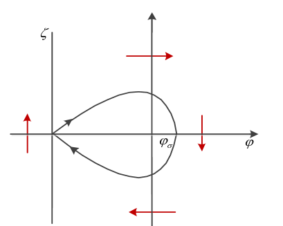
Figure 2.1: Phase portrait of system (2.3) for $\sigma=2$ with a homoclinic orbit.

This concludes the proof of existence of a homoclinic orbit starting and ending in the origin which corresponds to a solitary traveling wave solution of (2.2), cf. Figure 2.1. Hence, if $\sqrt{\frac{\sqrt{19}-4}{3}}<c<\frac{\sqrt{2}}{4}$ and $\sigma<c$, the $N_{\sigma}=(\varphi_{\sigma},0)$ lie in the right half-plane, there exists solitary traveling wave solutions of (1.1). If $\frac{\sqrt{2}}{4}<c<1$ and $\sigma>c$, the $N_{\sigma}=(\varphi_{\sigma},0)$ lie in the right half-plane, there exists solitary traveling wave solutions of the R-CH equation (1.1). ∎

Despite the fact that we are not able to explicitly solve (2.3), we can work out certain features of its solitary traveling wave solutions for $\sigma$ along the lines of ideas in [9], to qualitatively describe the wave profile. Let $\varphi$ be a solitary traveling wave solution of (2.3). We claim that $\varphi$ has a single maximum. To this end, multiply Eq.(2.2) by $\varphi_{x}$ and integrate over $\mathbb{R}$ yields

$$(c-\sigma)\varphi^{2}+\varphi^{3}+\frac{w_{1}}{6\alpha^{2}}\varphi^{4}+\frac{w_{2}}{10\alpha^{3}}\varphi^{5}+\left(\sigma-\frac{\beta_{0}}{\beta}\right)\varphi_{x}^{2}-\varphi\varphi_{x}^{2}=0,$$

which implies, if $\varphi\neq\sigma-\frac{\beta_{0}}{\beta}$, then

$$\varphi_{x}^{2}=\varphi^{2}\frac{m(\varphi)}{\varphi-\sigma+\frac{\beta_{0}}{\beta}},$$ (2.7)

where

$$m(\varphi)=\frac{w_{2}}{10\alpha^{3}}\varphi^{3}+\frac{w_{1}}{6\alpha^{2}}\varphi^{2}+\varphi+c-\sigma.$$

We can use the Cardano’s formula to find that the discriminant of this third-order polynomial is always negative, there has no multiple roots. We conclude that $\varphi$ vanishes precisely at the unique real root $\varphi_{m}$ of $m(\varphi)$, there exists a unique maximal wave height. Furthermore, this value $\varphi_{m}$ is attained at a single value of $\tau$. To see this, assume to the contrary that there exists an interval $(\tau_{1},\tau_{2})$ with $\varphi_{\tau}=\varphi_{m}$ for all $\tau\in(\tau_{1},\tau_{2})$. Hence, $\varphi_{m}$ would have to satisfy Eq.(2.2) in that interval, which reduces to

$$\frac{w_{2}}{4\alpha^{3}}\varphi_{m}^{3}+\frac{w_{1}}{3\alpha^{2}}\varphi_{m}^{2}+\frac{3}{2}\varphi_{m}+c-\sigma=0.$$

On the other hand, since $\varphi_{m}$ is a root of $m(\varphi)$, it must also satisfy the following equation

$$\frac{w_{2}}{10\alpha^{3}}\varphi_{m}^{3}+\frac{w_{1}}{6\alpha^{2}}\varphi_{m}^{2}+\varphi_{m}+c-\sigma=0,$$

but this is not possible. Also, assuming that there are two distinct and isolated values $\tau_{1},\tau_{2}$ with $\varphi(\tau_{1})=\varphi(\tau_{2})=\varphi_{m}$, there must be another maximum or minimum between these points since $\varphi$ decays for $|\tau|\rightarrow\infty$. Hence, there exists $\tau_{0}\in(\tau_{1},\tau_{2})$ where $\varphi^{\prime}(\tau_{0})=0$ but $\varphi(\tau_{0})\neq\varphi_{m}$ which contradicts the fact that $m(\varphi)$ has a unique real root. To determine $\varphi_{m}$, one can use again the Cardano’s formula to find that

$$\varphi_{m}=\sqrt[3]{-\kappa+\sqrt{D}}+\sqrt[3]{-\kappa-\sqrt{D}}-\frac{5\alpha w_{1}}{9w_{2}},$$

where

$$\kappa=\frac{125}{729}\frac{\alpha^{3}w_{1}^{3}}{w_{2}^{3}}-\frac{25}{9}\frac{\alpha^{4}w_{1}}{w_{2}^{2}}+5(c-\sigma)\frac{\alpha^{3}}{\ w_{2}},$$

and

$$D=\frac{1000}{27}\frac{\alpha^{9}}{w_{2}^{3}}-\frac{625}{243}\frac{\alpha^{8}w_{1}^{2}}{w_{2}^{4}}-\frac{250}{9}(c-\sigma)\frac{\alpha^{7}w_{1}}{w_{2}^{3}}+\frac{1250}{729}(c-\sigma)\frac{\alpha^{6}w_{1}^{3}}{w_{2}^{4}}+25(c-\sigma)^{2}\frac{\alpha^{6}}{w_{2}^{2}}.$$

We recall that $\varphi_{m}$ is the positive real root of the polynomial $m(\varphi)$ which displays a dependence on $\sigma$ only in the constant term. Hence, we have $m(\varphi,\sigma_{1})-m(\varphi,\sigma_{2})=\sigma_{2}-\sigma_{1}$ for $\sigma_{1}<\sigma_{2}$, the graph of $m(\varphi)$ is shifted upwards if we increase $\sigma$ and the zero of $m(\varphi)$ is shifted to the right. We will use the fact that $\varphi_{m}$ grows with $\sigma$ in the comparison of solitary wave profiles of different speeds below.

We claim that the wave profile is symmetric with respect to the vertical axis, that is, we have to show that $\varphi(\tau)$ is an even function of $\tau$. We recall (2.7) and regard $\varphi^{\prime}$ as a function of $\varphi$. This relation ensures that for every height of the profile $\varphi$ we get two values for the steepness of the wave at that point which only differ by sign. Hence the wave cannot be steeper on one side of the crest than on the other at the same height above the bed. To make this more precise, fix $\sigma>0$ and let $\varphi$ be a solution of (2.2) with crest point at $\tau=0$. Define the following function

$$\widetilde{\varphi}(\tau)=\begin{cases}\varphi(\tau)~{}~{}~{}~{}~{}\text{for}~{}~{}\tau\in(-\infty,0],~{}~{}~{}\\ \varphi(-\tau)~{}~{}~{}~{}\text{for }~{}~{}\tau\in[0,\infty),\end{cases}$$ (2.8)

which is even by construction. On interval $[0,\infty)$, both $\varphi$ and $\widetilde{\varphi}$ satisfy (2.2) and since $\varphi,\widetilde{\varphi}\in C^{1}$ in $\tau=0$, there exists a unique solution to the right of zero. Hence, $\varphi=\widetilde{\varphi}$ on $[0,\infty)$ and in particular $\varphi(\tau)=\widetilde{\varphi}(\tau)=\varphi(-\tau)$ on $[0,\infty)$ which proves the claim.

The solitary wave profile decays exponentially at infinity, which can be seen by performing a Taylor expansion of the right-hand side of (2.7) in $\varphi$ around zero. This yields

$$(\varphi^{\prime})^{2}=\varphi^{2}\frac{c-\sigma}{\frac{\beta_{0}}{\beta}-\sigma}+O(\varphi^{3})~{}~{}~{}~{}\text{for}~{}~{}|\tau|\rightarrow\infty,$$

and we conclude that

$$\varphi(\tau)=O\left(\text{exp}\left(-\sqrt{\frac{c-\sigma}{\frac{\beta_{0}}{\beta}-\sigma}}|\tau|\right)\right)~{}~{}~{}~{}\text{as}~{}~{}|\tau|\rightarrow\infty.$$ (2.9)

Note that the decay rate at infinity is given by the eigenvalue $\lambda^{-}_{0}$ of the Jacobian matrix at the fixed point $N_{0}$, which determines the angle at which the homoclinic orbit corresponding to the solitary wave solution leaves the origin.

It is also interesting to investigate variations of the wave profile $\varphi$ upon changing the wave speed $\sigma$. We show that two wave profiles with different speeds intersect precisely in two points. Indeed, let $\varphi$ be a solitary wave solution of (2.3) with crest point at $\tau=0$. Since our system displays an analytic dependence on the parameter $\sigma$, so does its solution and we can define the even function $f(\tau)=\partial_{\sigma}\varphi(\tau)$ for which we claim that it has precisely two zeros on $\mathbb{R}$. At $\tau=0$, $f$ is positive since the maximal height $\varphi(0)=\varphi_{m}$ is an increasing function of the wave speed $\sigma$. Furthermore, notice that the decay rate of $\varphi$ at infinity is faster for larger $\sigma$, since differentiating (2.9) with respect to $\sigma$ yields

$$\partial_{\sigma}\varphi=-\frac{|\tau|}{2}\sqrt{\frac{\frac{\beta_{0}}{\beta}-\sigma}{c-\sigma}}\frac{c-\frac{\beta_{0}}{\beta}}{(\frac{\beta_{0}}{\beta}-\sigma)^{2}}\varphi<0~{}~{}~{}~{}\text{for}~{}~{}|\tau|\rightarrow\infty,$$

we can obtain $f$ is negative for large $|\tau|$. Moreover, we show that the graph of $f$ is decreasing whenever it crosses the horizontal axis, i.e. if there exists $\tau_{0}>0$ such that $f(\tau_{0})=0$, then $f^{\prime}(\tau_{0})<0$. Indeed, differentiating (2.7) with respect to $\sigma$ gives

$$(f-1)(\varphi^{\prime})^{2}+2\varphi^{\prime}f^{\prime}\left(\varphi-\sigma-\frac{\beta_{0}}{\beta}\right)=2\varphi fm(\varphi)+\varphi^{2}f\left(\frac{3w_{2}}{10\alpha^{3}}\varphi^{2}+\frac{w_{1}}{3\alpha^{2}}\varphi+1\right)-\varphi^{2},$$

where ^′ denotes the derivative with respect to $\tau$ and we used that $\partial_{\sigma}\varphi=f^{\prime}$. Evaluating this equation at $\tau_{0}$, so that all the terms involving $f$ disappear, we find that

$$2\varphi^{\prime}f^{\prime}\left(\varphi-\sigma-\frac{\beta_{0}}{\beta}\right)=(\varphi^{\prime})^{2}-\varphi^{2}>0.$$

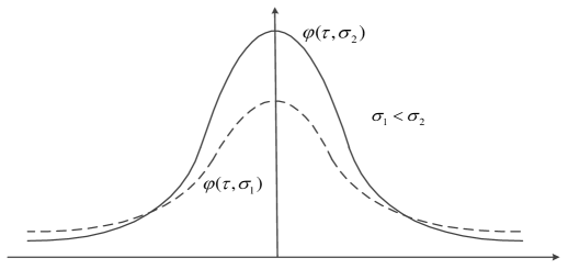
Figure 2.2: Solitary wave profiles with two different speeds.

The fact that the right-hand side is positive follows from (2.7), noting that $\frac{m(\varphi)}{\varphi-\sigma+\frac{\beta_{0}}{\beta}}<1$. Since the wave profile is decreasing to the right of the crest point, $\varphi^{\prime}(\tau_{0})<0$ and it follows from the above inequality that also $f(\tau_{0})<0$ which proves the claim. For the solitary wave solutions of (2.3) this means that, if we fix a wave speed $\sigma_{1}$ and find for the corresponding wave profile $\varphi(\tau,\sigma_{1})$ the unique value $\tau_{0}$ at which $f$ vanishes, then a wave profile $\varphi(\tau,\sigma_{2})$ corresponding to a higher speed $\sigma_{2}>\sigma_{1}$ lies above the original wave profile $\varphi(\tau,\sigma_{1})$ to the left of $\tau_{0}$ where $f$ is positive, and below $\varphi(\tau,\sigma_{1})$ to the right of $\tau_{0}$ where $f$ is negative. Since the wave profiles are symmetric with respect to the vertical axis, the same is true on the other side of the crest point, cf. Figure 2.2.

3 Stability of Solitary Waves

The main goal of this section is to prove that solitary traveling wave solutions of the R-CH equation (1.1) are orbitally stable.

If we define the orbit of a function $\varphi$ to be the set $O(\varphi)=\{\varphi(\cdot,x_{0}),x_{0}\in\mathbb{R}\}$, a solitary wave of the R-CH equation (1.1) is called orbitally stable if profiles near its orbit remain at all later times near the orbit. More precisely:

Definition 3.1.

(Orbital stability) The solitary wave $\varphi$ of the R-CH equation (1.1) is stable if for every $\varepsilon>0$ there exists $\gamma>0$ such that if $u\in C([0,T)$; $H^{2}(\mathbb{R}))$ for some $0<T\leq\infty$ is a solution to (1.1) with $||u(0)-\varphi||_{H^{2}}\leq\gamma$, then for every $t\in[0,T)$, we have

$$\underset{\xi\in\mathbb{R}}{\inf}||u(t,.)-\varphi(.-\xi)||_{H^{2}}\leq\varepsilon.$$

Otherwise, the solution is called unstable.

The verification of orbital stability relies strongly on a method introduced by Grillakis-Shatah-Strauss [26] and essentially follows from a theorem presented therein. To this end, we state the following assumptions:
  
(a) For every $u_{0}\in H^{s}(\mathbb{R})$, $s>3/2$, there exists a solution $u$ of Eq.(1.1) in $[0,T)$ such that $u(0)=u_{0}$ where $u\in C([0,T);H^{s}(\mathbb{R})\cap C^{1}[0,T);L^{2}(\mathbb{R}))$. Furthermore, there exist functionals $E(u)$ and $F(u)$ which are conserved for solutions of (1.1).
  
(b) For every $\sigma\in(0,\infty)$, there exists a traveling wave solution $\varphi\in H^{2}$ of Eq.(1.1), where $\varphi>0$ and $\varphi_{x}\not\equiv 0$. The mapping $\sigma\mapsto\varphi(x-\sigma t)$ is $C^{1}((0,\infty);H^{2})$. Moreover $\sigma E^{\prime}(\varphi)-F^{\prime}(\varphi)$, where $E^{\prime}$ and $F^{\prime}$ are the variational derivatives of $E$ and $F$, respectively.
 
(c) For every $\sigma\in(0,\infty)$, the linearized Hamiltonian operator around $\varphi$ defined by $$H_{\sigma}:H^{1}(\mathbb{R})\rightarrow H^{-1}(\mathbb{R}),~{}~{}~{}~{}H_{\sigma}=\sigma E^{\prime\prime}(\varphi)-F^{\prime\prime}(\varphi),$$ has exactly one negative simple eigenvalue, its kernel is spanned by $\varphi_{x}$ and the rest of its spectrum is positive and bounded away from zero.

Theorem 3.1.

(See [26]) Under above assumptions (a), (b) and (c), a solitary traveling wave solution $\varphi(x-\sigma t)$ of Eq.(1.1) is stable if and only if the scalar function

$$d(\sigma)=\sigma E(\varphi)-F(\varphi).$$ (3.1)

is convex in a neighborhood of $\sigma$.

The following theorem is important to determine the sign of $d^{\prime\prime}(\sigma)$.

Theorem 3.2.

(See [27]) Let

$$G_{b}(x)=g_{n}(b)x^{n}+g_{n-1}(b)x^{n-1}+\cdot\cdot\cdot+g_{1}(b)x+g_{0}(b)$$

be a family of real polynomials depending also polynomially on a real parameter $b$. If the following three conditions are met, then for all $b\in I$, $G_{b}(x)>0$. Suppose that there exists an open interval $I\subset\mathbb{R}$ such that:
  
(i) There is some $b_{0}\in I$, such that $G_{b_{0}}(x)>0$;
 
(ii) For all $b\in I$, $\Delta_{x}(G_{b})\neq 0$;
 
(iii) For all $b\in I$, $g_{n}(b)\neq 0$.

As usual, we write $\Delta_{x}(G)$ to denote the discriminant of a polynomial $G(x)=a_{n}x^{n}+\cdot\cdot\cdot+a_{1}x+a_{0}$, that is,

$$\Delta_{x}(G)=(-1)^{\frac{n(n-1)}{2}}\frac{1}{a_{n}}\text{Res}\left(G(x),G^{\prime}(x)\right),$$

where $\text{Res}(G,G^{\prime})$ is the resultant of $G$ and $G^{\prime}$.

In order to discuss the stability of solitary waves, we will show that the problem falls within the framework of the general approach to nonlinear stability provided by [26]. We compute the first and second variational derivatives of the conserved quantities $E$ and $F$, which are given by

$$E^{\prime}(u)v=(u-u_{xx},v),$$

$$E^{\prime\prime}(u)v=(I-\partial_{x}^{2},v),$$

$$F^{\prime}(u)v=\left(cu+\frac{3}{2}u^{2}-\frac{\beta_{0}}{\beta}u_{xx}+\frac{w_{1}}{3\alpha^{2}}u^{3}+\frac{w_{2}}{4\alpha^{3}}u^{4}-\frac{1}{2}u_{x}^{2}-uu_{xx},v\right),$$

and

$$F^{\prime\prime}(u)v=\left(c+3u-\frac{\beta_{0}}{\beta}\partial_{x}^{2}+\frac{w_{1}}{\alpha^{2}}u^{2}+\frac{w_{2}}{\alpha^{3}}u^{3}-u_{x}\partial_{x}-u\partial_{x}^{2}-u_{xx},v\right).$$

In terms of the functionals $E$ and $F$, Eq.(2.2) can be written as

$$\sigma E^{\prime}(\varphi)-F^{\prime}(\varphi)=0,$$

where $E^{\prime}$ and $F^{\prime}$ are the Fréchet derivatives of $E$ and $F$, respectively. The linearized Hamiltonian operator $H_{\sigma}$ of $(\sigma E^{\prime}-F^{\prime})$ around $\varphi$ is defined by

$$H_{\sigma} =\sigma E^{\prime\prime}(\varphi)-F^{\prime\prime}(\varphi)$$

$$=-\left(\sigma-\frac{\beta_{0}}{\beta}-\varphi\right)\partial_{x}^{2}-3\varphi-\frac{w_{1}}{\alpha^{2}}\varphi^{2}+\sigma+\frac{w_{2}}{\alpha^{3}}\varphi^{3}+\varphi_{xx}-c$$

$$=-\partial_{x}\left(\sigma-\frac{\beta_{0}}{\beta}-\varphi\right)\partial_{x}+\sigma-c-3\varphi-\frac{w_{1}}{\alpha^{2}}\varphi^{2}+\frac{w_{2}}{\alpha^{3}}\varphi^{3}+\varphi_{xx}.$$ (3.2)

Therefore, we can write the spectral equation $H_{\sigma}v=\lambda v$ as the Sturm-Liouville problem

$$-(Pv_{x})_{x}+(Q-\lambda)v=0,$$

where

$$P(x)=\sigma-\frac{\beta_{0}}{\beta}-\varphi,~{}~{}Q(x)=\sigma-c-3\varphi-\frac{w_{1}}{\alpha^{2}}\varphi^{2}+\frac{w_{2}}{\alpha^{3}}\varphi^{3}+\varphi_{xx}.$$

Recall that any regular Sturm-Liouville system has an infinite sequence of real eigenvalues $\lambda_{0}<\lambda_{1}<\lambda_{2}<\cdot\cdot\cdot$ with $\lim\limits_{n\to\infty}\lambda_{n}=\infty$ (see [5]). The eigenfunction $v_{n}(x)$ belonging to the eigenvalue $\lambda_{n}$ is uniquely determined up to a constant factor and has exactly $n$ zeros. Furthermore, observe that $H_{\sigma}$ is a self-adjoint, second order differential operator. Therefore its eigenvalues $\lambda$ are real and simple, and its essential spectrum is given by $[\sigma-c,\infty)$ in view of the fact that $\lim\limits_{x\to\infty}{\rm\inf}~{}Q(x)=\sigma-c$ ( see [19]). It is straightforward to verify that (2.2) is equivalent to $H_{\sigma}(\varphi_{x})=0$. Furthermore, $\varphi_{x}$ has exactly one zero on $\mathbb{R}$ in view of the fact that the solitary wave solutions of (2.2) have a unique maximum. We conclude that there is exactly one negative eigenvalue, and the rest of the spectrum is positive and bounded away from zero, which proves the claim.

Under the assumptions (a), (b) and (c), it is according to Theorem 3.1 that the stability would be ensured by the convexity of the scalar function and differentiating with respect to $\sigma$ and taking equation (3.1) into account, we find that

$$d^{\prime}(\sigma)=E(\varphi)+\left(\sigma E^{\prime}(\varphi)-F^{\prime}(\varphi),\partial_{\sigma}\varphi\right)=E(\varphi).$$ (3.3)

In the following theorem, we prove that $d^{\prime\prime}(\sigma)>0$ to infer stability of $\varphi$.

Theorem 3.3.

The energy $E=d^{\prime}(\sigma)$ is an increasing function of the wave speed $\sigma$. Therefore, all solitary traveling wave solutions of (1.1) are stable.

Proof.

Let $\varphi$ be a solitary traveling wave solution of (1.1). We notice that

$$\varphi_{x}^{2}=\varphi^{2}\frac{\frac{w_{2}}{10\alpha^{3}}\varphi^{3}+\frac{w_{1}}{6\alpha^{2}}\varphi^{2}+\varphi+c-\sigma}{\varphi-\sigma+\frac{\beta_{0}}{\beta}},$$

and that it is symmetric with respect to the crest. Therefore, $\varphi_{x}<0$ on $(0,\infty)$, we have

$$\varphi=-\varphi_{x}\sqrt{\frac{S(\varphi,\sigma)}{Y(\varphi,\sigma)}},$$

where

$$S(\varphi,\sigma)=\frac{w_{2}}{10\alpha^{3}}\varphi^{3}+\frac{w_{1}}{6\alpha^{2}}\varphi^{2}+\varphi+c-\sigma$$

and

$$Y(\varphi,\sigma)=\varphi-\sigma+\frac{\beta_{0}}{\beta}.$$

Thus, we have

$$d^{\prime}(\sigma) =\frac{1}{2}\int_{\mathbb{R}}(\varphi+\varphi_{x}^{2})dx=\int_{0}^{\infty}\varphi^{2}\left(1+\frac{S}{Y}(\varphi,\sigma)\right)dx$$

$$=-\int_{0}^{\infty}\varphi\varphi_{x}\left(\frac{S+Y}{\sqrt{SY}}(\varphi,\sigma)\right)dx$$

$$=\int_{0}^{h(\sigma)}y\left(\frac{S+Y}{\sqrt{SY}}(y,\sigma)\right)dy.$$ (3.4)

In the equality (3) we have performed the change of variables $y=\varphi(x)$ and used the fact that $\varphi$ has a unique maximum $h(\sigma)$, which corresponds to the unique real root of $S(\varphi,\sigma)$. Denoting $H=h(\sigma)$, we find that

$$\sigma=h^{-1}(H)=\frac{w_{2}}{10\alpha^{3}}H^{3}+\frac{w_{1}}{6\alpha^{3}}H^{2}+H+c,$$

which allows us to rewrite (3) as

$$U(H) =\int_{0}^{H}y\left(\frac{S+Y}{\sqrt{SY}}\left(y,h^{-1}(H)\right)\right)dy$$

$$=\int_{0}^{1}Hz\left(\frac{S+Y}{\sqrt{SY}}\left(Hz,h^{-1}(H)\right)\right)dz,$$

where we have performed the change of variables $y=Hz$. This improper integral is well defined on $(0,1)$ since the polynomials in the square root are positive in this interval, and the integrand becomes singular only when $z=1$. Now, denote the integrand by $f(z,H)$ and let $I=[H_{1},H_{2}]$ with $H_{1}>0$, so that we can view $U(H)=\int_{0}^{1}f(z,H)dz$ as a parameter integral. Observe that $f(\cdot,H)\in L^{1}(0,1)$ for all $H\in I$, and $f(z,\cdot)\in C^{1}(I)$ for all $z\in(0,1)$. Furthermore, we claim that there exists a function $g\in L^{1}(0,1)$ such that $|\partial_{H}f(z,H)|\leq g(z)$ for all $(z,H)\in(0,1)\times I$. Indeed,

$$f(z,H)=H^{2}z\left(\frac{S+Y}{\sqrt{SY}}\left(Hz,h^{-1}(H)\right)\right),$$

where

$$S\left(Hz,h^{-1}(H)\right)=H(1-z)\left[\frac{w_{2}}{10\alpha^{3}}H^{2}(1+z+z^{2})+\frac{w_{1}}{6\alpha^{2}}H(1+z)+1\right],$$

and

$$Y\left(Hz,h^{-1}(H)\right)=-c-\frac{\beta_{0}}{\beta}+H(z-1)-\frac{w_{1}}{6\alpha^{2}}H^{2}-\frac{w_{2}}{10\alpha^{3}}H^{3}.$$

Differentiating $f(z,H)$ with respect to $H$, we can find a positive constant $k$ depending only on $I$ such that

$$|\partial_{H}U(H)|\leq k\frac{1}{\sqrt{1-z}},$$

for $z\in(0,1)$ and $H\in I$. Let $g(z)=\frac{k}{\sqrt{1-z}}$ and observe that $g(z)\in L^{1}(0,1)$ which proves the claim. In view of the theorem on differentiation of parameter integrals in [21], we obtain

$$\partial_{H}U(H)=\int_{0}^{1}\partial_{H}f(z,H)dz.$$

Since the choice of $I$ was arbitrary, we can extend this result to all $H\in(0,\infty)$. Notice that $H=h(\sigma)$, then

$$d^{\prime\prime}(\sigma)=\partial_{H}U(H)h^{\prime}(\sigma),$$

where $h^{\prime}(\sigma)>0$ denotes the derivative of amplitude $h$ with respect to wave speed $\sigma$. To this end, let

$$A=\frac{w_{2}}{10\alpha^{3}}~{}~{}~{}~{}B=\frac{w_{1}}{6\alpha^{2}}~{}~{}~{}~{}K=\frac{\beta_{0}}{\beta},$$

consider the integrand of this expression and notice that it may be rewritten as

$$\partial_{H}U(H)=\frac{H^{2}z(1-z)N(z,H)}{\sqrt{(SY)^{3}}},$$

where

$$\begin{split}N(z,H)=&\frac{1}{2}(4\,A^{3}\,H^{8}\,z^{5}+4\,A^{3}\,H^{8}\,z^{4}+4\,A^{3}\,H^{8}\,z^{3}+5\,A^{2}\,B\,H^{7}\,z^{5}+12\,A^{2}\,B\,H^{7}\,z^{4}\\ &+12\,A^{2}\,B\,H^{7}\,z^{3}+2\,A^{2}\,B\,H^{7}\,z^{2}-6\,A^{2}\,H^{6}\,z^{6}+12\,A^{2}\,H^{6}\,z^{3}-7\,A^{2}\,H^{5}\,K\,z^{5}\\ &-7\,A^{2}\,H^{5}\,K\,z^{4}-7\,A^{2}\,H^{5}\,K\,z^{3}+2\,A^{2}\,H^{5}\,K\,z^{2}+2\,A^{2}\,H^{5}\,K\,z+2\,A^{2}\,H^{5}\,K\\ &+7\,A^{2}\,H^{5}\,c\,z^{5}+7\,A^{2}\,H^{5}\,c\,z^{4}+7\,A^{2}\,H^{5}\,c\,z^{3}-2\,A^{2}\,H^{5}\,c\,z^{2}-2\,A^{2}\,H^{5}\,c\,z\\ &-2\,A^{2}\,H^{5}\,c+9\,A\,B^{2}\,H^{6}\,z^{4}+12\,A\,B^{2}\,H^{6}\,z^{3}+6\,A\,B^{2}\,H^{6}\,z^{2}-11\,A\,B\,H^{5}\,z^{5}\\ &+14\,A\,B\,H^{5}\,z^{3}+8\,A\,B\,H^{5}\,z^{2}-13\,A\,B\,H^{4}\,K\,z^{4}-13\,A\,B\,H^{4}\,K\,z^{3}\\ &-4\,A\,B\,H^{4}\,K\,z^{2}+2\,A\,B\,H^{4}\,K\,z+2\,A\,B\,H^{4}\,K+13\,A\,B\,H^{4}\,c\,z^{4}\\ &+13\,A\,B\,H^{4}\,c\,z^{3}+4\,A\,B\,H^{4}\,c\,z^{2}-2\,A\,B\,H^{4}\,c\,z-2\,A\,B\,H^{4}\,c-8\,A\,H^{4}\,z^{4}\\ &+8\,A\,H^{4}\,z^{3}-9\,A\,H^{3}\,K\,z^{3}+9\,A\,H^{3}\,c\,z^{3}+A\,H^{2}\,K^{2}\,z^{2}+A\,H^{2}\,K^{2}\,z\\ &+A\,H^{2}\,K^{2}-2\,A\,H^{2}\,K\,c\,z^{2}-2\,A\,H^{2}\,K\,c\,z-2\,A\,H^{2}\,K\,c+A\,H^{2}\,c^{2}\,z^{2}\\ &+A\,H^{2}\,c^{2}\,z+A\,H^{2}\,c^{2}+4\,B^{3}\,H^{5}\,z^{3}+4\,B^{3}\,H^{5}\,z^{2}-5\,B^{2}\,H^{4}\,z^{4}+10\,B^{2}\,H^{4}\,z^{2}\\ &-6\,B^{2}\,H^{3}\,K\,z^{3}-6\,B^{2}\,H^{3}\,K\,z^{2}+6\,B^{2}\,H^{3}\,c\,z^{3}+6\,B^{2}\,H^{3}\,c\,z^{2}-6\,B\,H^{3}\,z^{3}\\ &+6\,B\,H^{3}\,z^{2}-6\,B\,H^{2}\,K\,z^{2}-2\,B\,H^{2}\,K+6\,B\,H^{2}\,c\,z^{2}+2\,B\,H^{2}\,c+2\,B\,H\,K^{2}\,z\\ &+2\,B\,H\,K^{2}-4\,B\,H\,K\,c\,z-4\,B\,H\,K\,c+2\,B\,H\,c^{2}\,z+2\,B\,H\,c^{2}\\ &+2\,H\,K\,z-2\,H\,K-2\,H\,c\,z+2\,H\,c+3\,K^{2}-6\,K\,c+3\,c^{2}).\end{split}$$

In view of the fact that $z\in(0,1)$ and $H\in(0,\infty)$, we have to prove that $N(z,H)\geq 0$. We will use a result for one-parameter families of polynomials in one variable by [27] which ensures that the polynomials do not change sign. We first perform the change of variables $z=\frac{x^{2}}{1+x^{2}}$ and $H=b^{2}$, which maps the strip $(0,1)\times(0,\infty)$ into the whole plane. Since the denominator of the resulting expression is everywhere positive, we only consider the numerator which is of the form

$$G_{b}(x)=g_{12}(b)x^{12}+g_{10}(b)x^{10}+\cdot\cdot\cdot+g_{2}(b)x^{2}+g_{0}(b),$$ (3.5)

where the $g_{i}(i=0,2,4,6,8,10,12)$ (see Appendix) depend polynomially on the real parameter $b$. Using the Sturm method one can check that $G_{1}(x)>0$ on $\mathbb{R}$, which ensures that the assumption (i) in Theorem 3.2 is satisfied. Next, we compute the discriminant of $G_{b}(x)$ and find that it is nonzero, which ensures that the assumption (ii) in Theorem 3.2 is satisfied. Finally, we use the Sturm method once more to show that $g_{12}(b)>0$ for all $b\in\mathbb{R}$, which ensures that the assumption (iii) in Theorem 3.2 is satisfied. Hence, we may conclude that $G_{b}(x)>0$ on $\mathbb{R}$. In summary, this proves that $N(z,H)\geq 0$ and we have $d^{\prime\prime}(\sigma)>0$, this completes the proof of theorem. ∎

Appendix

The $g_{i}(i=0,2,4,6,8,10,12)$ in (3.5) are as follows

$$\begin{split}g_{0}(b)=&2\,c-2\,K+2\,B\,c-6\,K\,c+2\,A^{2}\,K+2\,B\,K^{2}+A\,c^{2}-2\,A^{2}\,c+2\,B\,c^{2}+3\,K^{2}+3\,c^{2}\\ &-2\,A\,B\,c-2\,A\,K\,c-4\,B\,K\,c+A\,K^{2}\,c,\end{split}$$

$$\begin{split}g_{2}(b)=&16\,A^{2}\,K\,b^{10}-16\,A^{2}\,b^{10}\,c+14\,A\,B\,K\,b^{8}-16\,A\,B\,b^{8}\,c+A\,K^{2}\,b^{4}\,c+7\,A\,K^{2}\,b^{4}\\ &-16\,A\,K\,b^{4}\,c+8\,A\,b^{4}\,c^{2}+14\,B^{2}\,b^{2}\,c^{2}+16\,B\,K^{2}\,b^{2}-12\,B\,K\,b^{4}-32\,B\,K\,b^{2}\,c\\ &+14\,B\,b^{4}\,c+2\,B\,b^{2}\,c^{2}+21\,K^{2}-2\,K\,b^{2}-42\,K\,c+12\,b^{2}\,c+21\,c^{2},\end{split}$$

$$\begin{split}g_{4}(b)=&2\,A^{2}\,B\,b^{14}+42\,A^{2}\,K\,b^{10}-42\,A^{2}\,b^{10}\,c+6\,A\,B^{2}\,b^{12}+36\,A\,B\,K\,b^{8}+8\,A\,B\,b^{10}\\ &-36\,A\,B\,b^{8}\,c+21\,A\,K^{2}\,b^{4}-42\,A\,K\,b^{4}\,c+21\,A\,b^{4}\,c^{2}+4\,B^{3}\,b^{10}-6\,B^{2}\,K\,b^{6}\\ &+10\,B^{2}\,b^{8}+6\,B^{2}\,b^{6}\,c+40\,B\,K^{2}\,b^{2}-36\,B\,K\,b^{4}-80\,B\,K\,b^{2}\,c+6\,B\,b^{6}+36\,B\,b^{4}\,c\\ &+40\,B\,b^{2}\,c^{2}+45\,K^{2}-20\,K\,b^{2}-90\,K\,c+20\,b^{2}\,c+45\,c^{2},\end{split}$$

$$\begin{split}g_{6}(b)=&4\,A^{3}\,b^{16}+20\,A^{2}\,B\,b^{14}+61\,A^{2}\,K\,b^{10}+12\,A^{2}\,b^{12}-61\,A^{2}\,b^{10}\,c+36\,A\,B^{2}\,b^{12}\\ &+31\,A\,B\,K\,b^{8}+46\,A\,B\,b^{10}-31\,A\,B\,b^{8}\,c+34\,A\,K^{2}\,b^{4}-9\,A\,K\,b^{6}-68\,A\,K\,b^{4}\,c\\ &+8\,A\,b^{8}+9\,A\,b^{6}\,c+34\,A\,b^{4}\,c^{2}+20\,B^{3}\,b^{10}-30\,B^{2}\,K\,b^{6}+40\,B^{2}\,b^{8}+30\,B^{2}\,b^{6}\,c\\ &+60\,B\,K^{2}\,b^{2}-64\,B\,K\,b^{4}-120\,B\,K\,b^{2}\,c+18\,B\,b^{6}+64\,B\,b^{4}\,c+60\,B\,b^{2}\,c^{2}\\ &+60\,K^{2}-20\,K\,b^{2}-120\,K\,c+20\,b^{2}\,c+60\,c^{2},\end{split}$$

$$\begin{split}g_{8}(b)=&16\,A^{3}\,b^{16}+60\,A^{2}\,B\,b^{14}+34\,A^{2}\,K\,b^{10}+36\,A^{2}\,b^{12}-34\,A^{2}\,b^{10}\,c+81\,A\,B^{2}\,b^{12}\\ &-26\,A\,B\,K\,b^{8}+90\,A\,B\,b^{10}+26\,A\,B\,b^{8}\,c+31\,A\,K^{2}\,b^{4}-27\,A\,K\,b^{6}-62\,A\,K\,b^{4}\,c\\ &+16\,A\,b^{8}+27\,A\,b^{6}\,c+31\,A\,b^{4}\,c^{2}+36\,B^{3}\,b^{10}-54\,B^{2}\,K\,b^{6}+55\,B^{2}\,b^{8}+54\,B^{2}\,b^{6}\,c\\ &+50\,B\,K^{2}\,b^{2}-66\,B\,K\,b^{4}-100\,B\,K\,b^{2}\,c+18\,B\,b^{6}+66\,B\,b^{4}\,c+50\,B\,b^{2}\,c^{2}+45\,K^{2}\\ &-10\,K\,b^{2}90\,K\,c+10\,b^{2}\,c+45\,c^{2},\end{split}$$

$$\begin{split}g_{10}(b)=&24\,A^{3}\,b^{16}+73\,A^{2}\,B\,b^{14}-12\,A^{2}\,K\,b^{10}+36\,A^{2}\,b^{12}+12\,A^{2}\,b^{10}\,c+78\,A\,B^{2}\,b^{12}\\ &-59\,A\,B\,K\,b^{8}+63\,A\,B\,b^{10}+59\,A\,B\,b^{8}\,c+15\,A\,K^{2}\,b^{4}-27\,A\,K\,b^{6}-30\,A\,K\,b^{4}\,c\\ &+8\,A\,b^{8}+27\,A\,b^{6}\,c+15\,A\,b^{4}\,c^{2}+28\,B^{3}\,b^{10}-42\,B^{2}\,K\,b^{6}+30\,B^{2}\,b^{8}+42\,B^{2}\,b^{6}\,c\\ &+22\,B\,K^{2}\,b^{2}-36\,B\,K\,b^{4}-44\,B\,K\,b^{2}\,c+6\,B\,b^{6}+36\,B\,b^{4}\,c+22\,B\,b^{2}\,c^{2}+18\,K^{2}\\ &-2\,K\,b^{2}-36\,K\,c+2\,b^{2}\,c+18\,c^{2},\end{split}$$

$$\begin{split}g_{12}(b)=&12\,A^{3}\,b^{16}+31\,A^{2}\,B\,b^{14}-15\,A^{2}\,K\,b^{10}+6\,A^{2}\,b^{12}+15\,A^{2}\,b^{10}\,c+27\,A\,B^{2}\,b^{12}\\ &-26\,A\,B\,K\,b^{8}+11\,A\,B\,b^{10}+26\,A\,B\,b^{8}\,c+3\,A\,K^{2}\,b^{4}-9\,A\,K\,b^{6}-6\,A\,K\,b^{4}\,c\\ &+9\,A\,b^{6}\,c+3\,A\,b^{4}\,c^{2}+8\,B^{3}\,b^{10}-12\,B^{2}\,K\,b^{6}+5\,B^{2}\,b^{8}+12\,B^{2}\,b^{6}\,c+4\,B\,K^{2}\,b^{2}\\ &-8\,B\,K\,b^{4}-8\,B\,K\,b^{2}\,c+8\,B\,b^{4}\,c+4\,B\,b^{2}\,c^{2}+3\,K^{2}-6\,K\,c+3\,c^{2}.\end{split}$$

Data availability statement

Data sharing not applicable to this article as no datasets were generated or analysed during the current study.

Conflict of interest

The authors declare that they have no conflict of interest.

References

- [1] Andronov A A, Leontovich E A, Gordon I I, Maier A G. Qualitative Theory of Second Order Dynamic Systems. John Wiley and Sons, New York, 1973.
- [2] Alber M S, Camassa R, Holm D D. The geometry of peaked solitons and billiard solutions of a class of integrable PDE’s. Letters in Mathematical Physics, 1994, 32(2): 137-151.
- [3] Bressan A, Constantin A. Global conservative solutions of the Camassa-Holm equation. Archive for Rational Mechanics and Analysis, 2007, 183(2): 215-239.
- [4] Bressan A, Constantin A. Global dissipative solutions of the Camassa-Holm equation. Analysis and Applications, 2007, 5(1): 1-27.
- [5] Birkhoff G, Rota G C. Ordinary Differential Equations. John Wiley and Sons, New York, 1998.
- [6] Chen R M, Gui G, Liu Y. On a shallow-water approximation to the Green-Naghdi equations with the Coriolis effect. Advances in Mathematics, 2018, 340: 106-137.
- [7] Constantin A, Johnson R S. The dynamics of waves interacting with the equatorial undercurrent. Geophysical and Astrophysical Fluid Dynamics, 2015, 109(4): 311-358.
- [8] Constantin A, Johnson R S. An exact, steady, purely azimuthal equatorial flow with a free surface. Journal of Physical Oceanography, 2016, 46(6): 1935-1945.
- [9] Constantin A, Strauss W A. Stability of the Camassa-Holm solitons. Journal of Nonlinear Science, 2002, 12: 415-422.
- [10] Constantin A, Strauss W A. Stability of peakons. Communications on Pure and Applied Mathematics, 2000, 53(5): 603-610.
- [11] Constantin A, Escher J. Wave breaking for nonlinear nonlocal shallow water equations. Acta Mathematica, 1998, 181(2): 229-243.
- [12] Constantin A, Escher J. Global existence and blow-up for a shallow water equation. Annali della Scuola Normale Superiore di Pisa-Classe di Scienze, 1998, 26(2): 303-328.
- [13] Constantin A. Existence of permanent and breaking waves for a shallow water equation: a geometric approach. Annales De L Institut Fourier, 2000, 50(2): 321-362.
- [14] Constantin A, Escher J. On the blow-up rate and the blow-up set of breaking waves for a shallow water equation. Mathematische Zeitschrift, 2000, 233(1): 75-91.
- [15] Camassa R, Holm D D. An integrable shallow water equation with peaked solitons. Physical Review Letters, 1993, 71(11): 1661-1664.
- [16] Cao C, Holm D D, Titi E S. Traveling wave solutions for a class of one-dimensional nonlinear shallow water wave models. Journal of Dynamics and Differential Equations, 2004, 16(1): 167-178.
- [17] Danchin R. A few remarks on the Camassa-Holm equation. Differential and Integral Equations, 2001, 14(8): 953-988.
- [18] Danchin R. A note on well-posedness for Camassa-Holm equation. Journal of Differential Equations, 2003, 192(2): 429-444.
- [19] Dunford N, Schwarz J T. Linear Operators. John Wiley and Sons, New York, London, 1963.
- [20] Da Silva P L, Freire I L. Well-posedness travelling waves and geometrical aspects of generalizations of the Camassa-Holm equation. Journal of Differential Equations, 2019, 267(9): 5318-5369.
- [21] Escher J, Amann H. Analysis. Birkhäuser, Basel, Boston, Berlin, 2001.
- [22] Fuchssteiner B, Fokas A S. Symplectic structures their Bäcklund transformations and hereditary symmetries. Physica D: Nonlinear Phenomena, 1981, 4(1): 47-66.
- [23] Fisher M, Schiff J. The Camassa-Holm equation: conserved quantities and the initial value problem. Physics Letters A, 1999, 259(5): 371-376.
- [24] Gui G, Liu Y, Sun J. A nonlocal shallow water model arising from the full water waves with the Coriolis effect. Journal of Mathematical Fluid Mechanics, 2019, 21(2): 1-30.
- [25] Gui G, Liu Y, Luo T. Model equations and traveling wave solutions for shallow water waves with the Coriolis effect. Journal of Nonlinear Science, 2019, 29(3): 993-1039.
- [26] Grillakis M, Shatah J, Strauss W A. Stability theory of solitary waves in the presence of symmetry. Journal of Functional Analysis, 1987, 74: 160-197.
- [27] Garcia-Saldana J D, Gasull A, Giacomini H. Bifurcation values for a family of planar vector fields of degree five. Discrete and Continuous Dynamical Systems, 2012, 35(2): 669-701.
- [28] Geyer A. Solitary traveling water waves of moderate amplitude. Journal of Nonlinear Mathematical Physics, 2012, 19: 104-115.
- [29] Li Y A, Olver P J. Well-posedness and blow-up solutions for an integrable nonlinearly dispersive model wave equation. Journal of Differential Equations, 2000, 162(1): 27-63.
- [30] Perko L. Differential Equations and Dynamical Systems. Springer, New York, 1991.
- [31] Tu X, Liu Y, Mu C. Existence and uniqueness of the global conservative weak solutions to the rotation-Camassa-Holm equation. Journal of Differential Equations, 2019, 266(8): 4864-4900.
- [32] Wang T, Yang S, Han X. Symmetric waves are traveling waves for the rotation-Camassa-Holm equation. Journal of Mathematical Fluid Mechanics, 2021, 23(3): 1-4.
- [33] Yang S. Generic regularity of conservative solutions to the rotational-Camassa-Holm equation. Journal of Mathematical Fluid Mechanics, 2020, 22(4): 1-11.
- [34] Zhang L. Non-uniform dependence and well-posedness for the rotation-Camassa-Holm equation on the torus. Journal of Differential Equations, 2019, 267(9): 5049-5083.