Thermodynamically ideal quantum-state inputs to any device

Abstract

We investigate and ascertain the ideal inputs to any finite-time thermodynamic process. We demonstrate that the expectation values of entropy flow, heat, and work can all be determined via Hermitian observables of the initial state. These Hermitian operators encapsulate the breadth of behavior and the ideal inputs for common thermodynamic objectives. We show how to construct these Hermitian operators from measurements of thermodynamic output from a finite number of effectively arbitrary inputs. Behavior of a small number of test inputs thus determines the full range of thermodynamic behavior from all inputs. For any process, entropy flow, heat, and work can all be extremized by pure input states—eigenstates of the respective operators. In contrast, the input states that minimize entropy production or maximize the change in free energy are non-pure mixed states obtained from the operators as the solution of a convex optimization problem. To attain these, we provide an easily implementable gradient descent method on the manifold of density matrices, where an analytic solution yields a valid direction of descent at each iterative step. Ideal inputs within a limited domain, and their associated thermodynamic operators, are obtained with less effort. This allows analysis of ideal thermodynamic inputs within quantum subspaces of infinite-dimensional quantum systems; it also allows analysis of ideal inputs in the classical limit. Our examples illustrate the diversity of ‘ideal’ inputs: Distinct initial states minimize entropy production, extremize the change in free energy, and maximize work extraction.

I Introduction

Throughout its history, thermodynamics primarily investigated the efficiency of various control processes for implementing a desired functionality. However, the complementary question of which initial physical states produce the best thermodynamic behavior remains relatively unexplored. Indeed, there is a historical reason for this: In equilibrium transformations, the system always stays infinitesimally close to equilibrium, so there is no sense in asking about alternative inputs to the process. Yet modern devices transform quantum and classical system rapidly. These finite-time nonequilibrium transformations have highly non-trivial initial-state dependence. Here we explore the ideal thermodynamic inputs to such devices, where the system can be arbitrarily far from equilibrium throughout the transformation.

The initial-state dependence of entropy production and associated thermodynamic quantities has been explored only recently in relation to the ideal inputs, via mismatch costs [1, 2, 3, 4]. However, the minimally dissipative input was only characterized in the case of reset processes [3, 4] and, even then, a construction was only given for qubits [3]. In the following, we constructively identify the thermodynamically ideal inputs for a much broader class of objectives, including heat minimization, maximizing work extraction, and maximizing gain in free energy. Moreover, the ideal inputs are characterized and constructively identified for systems of arbitrary finite dimensions, for any finite-time process. The results apply to both quantum and classical systems. The results thus apply broadly, from biology to electronics to cosmology, wherever finite-time thermodynamics is relevant.

II Overview of Framework

It is often desirable for a physical device to implement a fixed transformation on arbitrary input. For example, in quantum technology, we often want to construct a device that implements a prescribed completely positive and trace preserving (CPTP) map. The device can achieve this via a time-dependent protocol that partially controls the system’s Hamiltonian and its interactions with its environment. We assume that the control protocol and the initial state of the environment are fixed, while we are free to select the initial (mixed or pure) state of the system to input to our device. The initial joint state of the system–environment supersystem is then $\rho_{0}^{\text{tot}}=\rho_{0}\otimes\rho_{0}^{\text{env}}$. The joint system–baths supersystem evolves unitarily via $U_{t}$, such that the joint state at any later time $t$ is given as $\rho_{t}^{\text{tot}}=U_{t}\rho_{0}^{\text{tot}}U_{t}^{\dagger}$. The reduced states of the system and environment are given at any time by the appropriate partial trace of the joint state: $\rho_{t}=\text{tr}_{\text{env}}(\rho_{t}^{\text{tot}})$ and $\rho_{t}^{\text{env}}=\text{tr}_{\text{sys}}(\rho_{t}^{\text{tot}})$. Any CPTP transformation of the system can be achieved this way.

In the following sections, we will discover the thermodynamically ideal inputs to any such CPTP transformation. To achieve this, we first introduce thermodynamic operators in Sec. III, generalized Bloch vectors in Sec. IV, and thermodynamic vectors in Sec. V. We then show how to construct these thermodynamic vectors and operators from experimental observations in Sec. VI. This finally allows us to discuss and construct the thermodynamically ideal inputs in Secs. VII and VIII. Sec. IX shows how these results apply to restricted subspaces—which is important for understanding the classical limit, and for applying the results to low-energy subspaces of infinite-dimensional systems. Finally, the examples in Secs. X and XI illustrate physical implications of our results.

III Thermodynamic operators

Thermodynamic quantities like work, heat, and entropy flow are notoriously path-dependent quantities. Even their average values depend on the time-dependent control protocol and the time-dependent density matrices of system and environment. For example, the expectation value of entropy flow can very generally be calculated as

$$\braket{\Phi}_{\rho_{0}} =-k_{\text{B}}\int_{0}^{\tau}\text{tr}\bigl{(}\dot{\rho}_{t}^{\text{env}}\ln\bm{\pi}_{t}^{\text{env}}\bigr{)}\,dt~{},$$ (1)

where $\bm{\pi}_{t}^{\text{env}}$ is a tensor product of local-equilibrium reference states for the environment at time $t$. Familiar expressions like $\braket{\Phi}_{\rho_{0}}=\int\tfrac{\braket{\delta Q^{(b)}}}{T_{t}^{(b)}}\,dt$ and $\braket{\Phi}_{\rho_{0}}=\tfrac{\braket{Q^{(b)}}}{T_{0}^{(b)}}+\tfrac{\braket{Q^{(b^{\prime})}}}{T_{0}^{(b^{\prime})}}$ are special cases of Eq. (1), where $Q^{(b)}$ is the change in energy of bath $b$, and $T_{t}^{(b)}$ is the temperature of bath $b$ at time $t$. With $H_{t}$ as the time-dependent Hamiltonian of the system, similar integral expressions for work

$$\braket{W}_{\rho_{0}}=\int_{0}^{\tau}\text{tr}\bigl{(}\rho_{t}\dot{H}_{t}\bigr{)}\,dt$$ (2)

and heat absorbed by the system

$$\braket{Q}_{\rho_{0}}=\int_{0}^{\tau}\text{tr}\bigl{(}\dot{\rho}_{t}H_{t}\bigr{)}\,dt$$ (3)

are familiar centerpieces of the thermodynamic arsenal. In this path-dependent spirit, it has been famously emphasized that “work is not an observable” [5].

It is therefore perhaps surprising that the expectation values of work, heat, and entropy flow can all be determined via Hermitian observables of the initial state. As we show in App. A, since the above expectation values are all linear functionals of the initial density matrix of the system, they can be expressed as

$$\braket{\Phi}_{\rho_{0}}=\text{tr}(\rho_{0}\bm{\Phi})~{},\qquad\braket{W}_{\rho_{0}}=\text{tr}(\rho_{0}\mathcal{W})~{},\qquad\text{and}\quad\braket{Q}_{\rho_{0}}=\text{tr}(\rho_{0}\mathcal{Q})~{},$$ (4)

where $\bm{\Phi}$, $\mathcal{W}$, and $\mathcal{Q}$ are Hermitian operators, which we refer to as the expected-entropy-flow operator, expected-work operator, and expected-heat operator respectively. We will show that, for a general finite-time thermodynamic process, these thermodynamic operators can be constructed via experimental observations from a finite number of arbitrary inputs. The operators in turn reveal the special collection of initial states that minimize entropy flow, minimize heat, and maximize work extraction. The operators also allow direct calculation of thermodynamic expectation values from any initial state.

The expressions in Eq. (4) all clearly take the form

$$\braket{X}_{\rho_{0}} =\text{tr}(\rho_{0}\mathcal{X})~{},$$ (5)

which we will study in general. We will say that a thermodynamic quantity is ‘type-I’ when its expectation value can be expressed as a linear functional of the initial state $\text{tr}(\rho_{0}\mathcal{X})$, as in Eq. (5). As an added benefit of studying this general formulation, our methods can also be applied to reconstruct the Hamiltonian, the expected-change-of-energy operator, and infinitely many other linear operators that conform to this general linear structure for expectation values. If the expectation value is always real-valued, then $\mathcal{X}$ is guaranteed to be Hermitian (see Thm. 2.4.3 of Hassani [6]).

It is known that invasive measurements can change the expected value of work and other thermodynamic variables [7]. We emphasize that different measurement schemes must be treated as distinct quantum processes, since each implies a unique sequence of dynamic interventions. Accordingly, each measurement scheme induces its own set of thermodynamic operators. For example, in App. B, we address the two-point measurements (TPM) scheme, and give an explicit construction of the expected-TPM-work operator $\mathcal{W}_{\text{TPM}}$, for which

$$\braket{W_{\text{TPM}}}_{\rho_{0}}=\text{tr}(\rho_{0}\mathcal{W}_{\text{TPM}})~{}.$$ (6)

Indeed, for any measurement scheme—TPM [8], one-point measurement [9, 10, 11], or any other scheme—thermodynamic operators can be constructed, and our framework can be applied to identify both the breadth of behavior and the ideal inputs within the scheme.

It is important to note that each of these thermodynamic operators $\mathcal{X}$ contain all information needed for expectation values of the relevant thermodynamic quantity $X$, but do not contain the information that would be needed for expectation values of functions of the thermodynamic quantity, like $X^{2}$ or $e^{X}$. As a point of nomenclature, we note that this is not about whether the operators are ‘observable’, as has been suggested [5], but is rather an elementary fact about expectation values—$\braket{X}$ does not determine $\braket{f(X)}$. The source of insufficiency is simple to see if we take work as an example: The full work distribution of a process, whether classical or quantum, has support on a space much larger than the dimension $d$ of the system. Accordingly, the $d$ eigenvalues of the thermodynamic operator cannot represent the full probability distribution of the thermodynamic quantity. 

To address a final nuance, we note that a random variable $X$ in the quantum domain may depend on further specification of subensembles, since a density matrix can be decomposed in many ways [12]. Nevertheless, as discussed in App. C, all decompositions of the initial density matrix lead to the same expectation value for a fixed quantum process. Accordingly, our notation “$\braket{X}_{\rho_{0}}$” unambiguously refers to the expectation value of the relevant thermodynamic quantity $X$ for all possible decompositions of the quantum state.

Despite these caveats, the thermodynamic operators serve immense utility. Their $d$ eigenstates represent the only $d$ features that influence the expected value of the thermodynamic variable. Once inferred for a process, the thermodynamic operators tell the full breadth of expected behavior from any input, and identify the unique pure states leading to extremal behavior. Moreover, the performance of any of the infinitely many possible inputs can be calculated simply and directly from the thermodynamic operator, without needing to run a new experiment each time.

IV Generalized Bloch vector

We have promised that thermodynamic operators are the key to identifying thermodynamically ideal inputs to any process. It will be important then to be able to construct these operators. Our construction will lean on generalized Bloch vectors and related thermodynamic vectors, introduced in this and the next section respectively.

It is well known that the state of a qubit $\rho_{t}$ can be expressed via its Bloch vector $\vec{a}_{t}$:

$$\rho_{t}=I/2+\vec{a}_{t}\cdot\vec{\sigma}/2~{},$$ (7)

where $\vec{\sigma}=(\sigma_{x},\sigma_{y},\sigma_{z})$ is the vector of Pauli matrices. For a quantum system of arbitrary finite dimension—i.e., a qudit $\rho_{t}$ acting on a $d$-dimensional vector space $\mathcal{V}_{d}$—we achieve something similar via a slight adaptation of Ref. [13]. We choose any complete basis $(I/d,\Gamma_{1},\Gamma_{2},\dots\Gamma_{d^{2}-1})$ for linear operators acting on $\mathcal{V}_{d}$, such that the Hermitian operators $\Gamma_{n}$ are all traceless and mutually orthogonal, satisfying

$$\text{tr}(\Gamma_{n}) =0,\;\text{ and }$$ (8a)

$$\text{tr}(\Gamma_{m}\Gamma_{n}) =\eta\,\delta_{m,n}~{},$$ (8b)

where we will choose the normalizing constant to be $\eta=\tfrac{d-1}{d}$. Any density matrix then has a unique decomposition in the operator basis $\vec{\Gamma}=(\Gamma_{1},\Gamma_{2},\dots\Gamma_{d^{2}-1})$, described by the generalized Bloch vector $\vec{b}_{t}\in\mathbb{R}^{d^{2}-1}$ via

$$\rho_{t}=I/d+\vec{b}_{t}\cdot\vec{\Gamma}~{}.$$ (9)

Since the magnitude of the Bloch vector is $b_{t}=\sqrt{\frac{\text{tr}(\rho_{t}^{2})d-1}{d-1}}$, the density matrix represents a pure state iff the magnitude of its corresponding Bloch vector is one. For $d>2$, not all points in the Bloch ball correspond to physical states, but the set of all physical states is nevertheless a convex set—the convex hull of the pure states, which all lie on a $2(d-1)$-dimensional submanifold of the $(d^{2}-2)$-dimensional surface of the Bloch sphere [13].

For concreteness, we can choose the ordered operator basis to be a scaled ordering of generalized Gell-Mann matrices—the generators of SU($d$). See App. E for details. The standard Bloch vector is then recovered in the familiar two-dimensional case of a qubit, where then $\vec{\Gamma}=\vec{\sigma}/2=(\sigma_{x}/2,\,\sigma_{y}/2,\,\sigma_{z}/2)$ and $\eta=1/2$. Alternatively, App. F shows how to construct valid composite operator bases.

V Thermodynamic vectors

Leveraging the general Bloch decomposition Eq. (9) of the initial state, we find that we can express each expectation value in Eq. (4) as

$$\braket{X}_{\rho_{0}} =\braket{X}_{I/d}+\vec{b}_{0}\cdot\vec{x}~{},$$ (10)

where $\vec{x}\in\mathbb{R}^{d^{2}-1}$ is the relevant thermodynamic vector

$$\vec{x}=\text{tr}(\vec{\Gamma}\mathcal{X})~{}.$$ (11)

In particular, the thermodynamic vector could be the entropy-flow vector $\vec{\varphi}=\text{tr}(\vec{\Gamma}\bm{\Phi})$, the work vector $\vec{w}=\text{tr}(\vec{\Gamma}\mathcal{W})$, or the heat vector $\vec{q}=\text{tr}(\vec{\Gamma}\mathcal{Q})$.

Conversely, the thermodynamic operators can be constructed from the thermodynamic vectors:

$$\mathcal{X}=\braket{X}_{I/d}I+\vec{x}\cdot\vec{\Gamma}/\eta~{}.$$ (12)

Using Eqs. (8a) and (8b), it is easy to verify that Eq. (12) satisfies $\text{tr}(\rho_{0}\mathcal{X})=\braket{X}_{I/d}+\vec{b}_{0}\cdot\vec{x}$.

In the next sections, we show how both $\braket{X}_{I/d}$ and the thermodynamic vector $\vec{x}$ can be obtained linear algebraically from experimental measurements of thermodynamic output from a finite number of almost arbitrary inputs . Via Eq. (12), this allows us to experimentally reconstruct the thermodynamic operators from observations of any process.

VI Constructing thermodynamic vectors and operators from observations

Suppose an experimentalist has an apparatus to transform the state of a finite-dimensional quantum system. (We will address infinite-dimensional systems in Sec. IX.) This experimentalist measures the expectation value of the thermodynamic random variable $X$ that results from each of $d^{2}$ linearly independent inputs to their device. I.e., they record the average quantity from each of the initial states $(\rho_{0}^{(n)})_{n=1}^{d^{2}}$ with corresponding generalized Bloch vectors $(\vec{b}_{0}^{(n)})_{n=1}^{d^{2}}$. Note that the generalized Bloch vectors can be obtained as $\vec{b}_{0}^{(n)}=\text{tr}(\rho_{0}^{(n)}\vec{\Gamma})/\eta$. From Eq. (10), we see that

$$\underbrace{\begin{bmatrix}1&\vec{b}_{0}^{(1)}\\ 1&\vec{b}_{0}^{(2)}\\ \vdots&\vdots\\ 1&\vec{b}_{0}^{(d^{2})}\end{bmatrix}}_{\eqqcolon B}\begin{bmatrix}\braket{X}_{I/d}\\ \vec{x}\end{bmatrix} =\begin{bmatrix}\braket{X}_{\rho_{0}^{(1)}}\\ \braket{X}_{\rho_{0}^{(2)}}\\ \vdots\\ \braket{X}_{\rho_{0}^{(d^{2})}}\end{bmatrix}$$ (13)

Notice that the $B$ matrix defined in Eq. (13) is invertible since the $d^{2}$ initial states are all linearly independent. Hence, with the $d^{2}$ measurements in hand and some simple linear algebra, we can find both (i) the expectation value from the reference input $\braket{X}_{I/d}$ and (ii) the input-independent thermodynamic vector $\vec{x}$:

$$\begin{bmatrix}\braket{X}_{I/d}\\ \vec{x}\end{bmatrix} =B^{-1}\begin{bmatrix}\braket{X}_{\rho_{0}^{(1)}}\\ \braket{X}_{\rho_{0}^{(2)}}\\ \vdots\\ \braket{X}_{\rho_{0}^{(d^{2})}}\end{bmatrix}~{}.$$ (14)

$\braket{X}_{I/d}$ and $\vec{x}$ can now be used in Eq. (12) to construct the thermodynamic operator of interest: $\mathcal{X}=\braket{X}_{I/d}I+\vec{x}\cdot\vec{\Gamma}/\eta$. This constitutes a type of ‘operator tomography’, which is distinct but reminiscent of both quantum-state tomography and process tomography.

We are now equipped to identify and construct the thermodynamically ideal inputs to any device.

VII Ideal inputs for type-I objectives

Recall that a thermodynamic quantity is ‘type-I’ when its expectation value can be expressed as a linear functional of the initial state $\text{tr}(\rho_{0}\mathcal{X})$. It is often desirable to minimize or maximize type-I quantities, e.g., to minimize heat or maximize work extraction.

An immediate observation can be drawn from Eq. (5) for any finite-dimensional quantum system, by considering the spectral decomposition of the bounded operator $\mathcal{X}=\sum_{n=1}^{d}\lambda_{n}\ket{v_{n}}\!\bra{v_{n}}$, where $\Lambda_{\mathcal{X}}=(\lambda_{n})_{n}$ is the tuple of $\mathcal{X}$’s eigenvalues with corresponding eigenstates $V_{\mathcal{X}}=(\ket{v_{n}})_{n}$.

Theorem 1.

There is always a pure-state input that extremizes the expectation value of type-I quantities $\braket{X}_{\rho_{0}}=\text{tr}(\rho_{0}\mathcal{X})$. This pure state corresponds to an eigenstate of the thermodynamic operator $\mathcal{X}$ with extremal eigenvalue.

For example: there is always a pure-state input that minimizes heat; there is always a pure-state input that maximizes heat; there is always a pure-state input that minimizes entropy flow; and so on.

The implications are important and somewhat surprising. For instance, consider the work extracted $W_{\text{extracted}}=-W$ during a finite-time cyclic work-extraction protocol from a finite-dimensional quantum system. Thm. 1 asserts that maximal work can be extracted from the pure-state input $\ket{w_{\text{min}}}\in\text{argmin}_{\ket{v}\in V_{\mathcal{W}}}\bigl{\{}\braket{v}{\mathcal{W}}{v}\bigr{\}}$. When the minimal-eigenvalue eigenspace of $\mathcal{W}$ is degenerate, maximal work extraction can be achieved by both pure and mixed inputs. In contrast, as we will see later, the state that minimizes entropy production is generically a mixed state. Therefore, pure-state inputs that maximize work extraction imply non-minimal entropy production. Similarly, pure-state inputs that minimize heat imply non-minimal entropy production.

One broad lesson from this analysis is that maximizing work extraction, minimizing heat, minimizing entropy production, etc., are all distinct concepts that should not be conflated. There is a great diversity in optimality among different thermodynamic goals. This will be emphasized again in our first example in Sec. X.

It is worth noting that the smallest and largest eigenvalues of each thermodynamic operator demarcate the range of corresponding expectation values that can be achieved via alternative inputs:

$$\braket{X}_{\rho_{0}}\in[\min(\Lambda_{\mathcal{X}}),\,\max(\Lambda_{\mathcal{X}})]~{}.$$ (15)

All values in this continuous range are achievable by some input.

VIII Ideal inputs for type-II objectives

Not all thermodynamic expectation values can be expressed like Eq. (5) as a linear functional of the initial state. In particular, entropy production, reduction in nonequilibrium free energy, and change in entropy all have expectation values that are nonlinear functions of the initial state. However, in each of these three cases, the nonlinearity is of the same form, since it derives from the change of von Neumann entropy $S(\rho)=-\text{tr}(\rho\ln\rho)$. Accordingly, the initial states that extremize this second class of thermodynamic quantities all share similar features.

The expectation value of entropy production, $\braket{\Sigma}_{\rho_{0}}=\braket{\Phi}_{\rho_{0}}+k_{\text{B}}\Delta S(\rho_{t})$, plays a central role in nonequilibrium thermodynamics. When the environment begins in local equilibrium, and is uncorrelated with both itself and the system, then the famous Second Law of thermodynamics is valid: $\braket{\Sigma}_{\rho_{0}}\geq 0$. In the appropriate circumstances, entropy production alternatively can be expressed as the work performed beyond the change in nonequilibrium free energy $T\braket{\Sigma}_{\rho_{0}}=\braket{W}_{\rho_{0}}-\Delta\mathcal{F}_{t}$, where $T$ is the initial temperature of the environment.

The expectation values of (i) entropy production, (ii) change in free energy, and (iii) change in entropy are each proportional to

$$f_{\rho_{0}}^{(\mathcal{X})}\coloneqq\text{tr}(\rho_{0}\mathcal{X})+S(\rho_{\tau})-S(\rho_{0})$$ (16)

for the appropriate linear operators $\mathcal{X}$. We will say that a thermodynamic quantity is ‘type-II’ when its expectation value is proportional to $f_{\rho_{0}}^{(\mathcal{X})}$ for some linear operator $\mathcal{X}$ and some positive constant of proportionality. In particular,

$$\braket{\Sigma}_{\rho_{0}}=k_{\text{B}}f_{\rho_{0}}^{(\bm{\Phi}/k_{\text{B}})}\quad\text{and}\quad\Delta S_{t}=f_{\rho_{0}}^{(0)}\quad\text{and}\quad-\Delta\mathcal{F}_{t}=k_{\text{B}}Tf_{\rho_{0}}^{(-(\mathcal{Q}+\mathcal{W})/k_{\text{B}}T)}~{}.$$ (17)

VIII.1 General processes

VIII.1.1 Inputs that minimize type-II functions

Theorem 2.

An initial state that locally minimizes a type-II quantity also globally minimizes it.

This is because type-II quantities are convex in the initial state.

For general processes, the nonlinearity of type-II objectives makes it difficult to find a closed-form expression for ideal inputs $\text{argmin}_{\rho_{0}}f_{\rho_{0}}^{(\mathcal{X})}$. Nevertheless, since type-II quantities are convex in the initial state, any number of simple algorithms, including gradient descent and related variations, are guaranteed to converge to the ideal input upon iteration. By convexity, a local minimum in $f_{\rho_{0}}^{(\mathcal{X})}$, when minimizing over the set of density matrices, is also the global minimum.

However, constrained optimization—restricting to the set of density matrices in this case—is non-trivial. Although some techniques for gradient descent on the manifold of density matrices have been developed—see, e.g., Refs. [14, 15] and references therein—we found a more direct solution to our problem, which we provide in this section. Our resulting algorithm for gradient descent provides a quantum generalization of the Frank–Wolfe algorithm [16], with a simple analytically solvable direction for descent at each step.

Using techniques introduced in Ref. [2], we can analytically calculate the gradient of type-II expectation values around any initial state, given any parametrization of the state space. If we consider arbitrary infinitesimal changes in the initial generalized Bloch vector, then the partial derivative of $f_{\rho_{0}}^{(\mathcal{X})}$, with respect to each Bloch-vector component, can be expressed as

$$\frac{\partial}{\partial{b_{0}}_{m}}f_{\rho_{0}}^{(\mathcal{X})}=\text{tr}(\Gamma_{m}\mathcal{X})+\text{tr}(\Gamma_{m}\ln\rho_{0})-\text{tr}\Bigl{\{}\text{tr}_{\text{env}}\bigl{[}U(\Gamma_{m}\otimes\rho_{0}^{\text{env}})U^{\dagger}\bigr{]}\ln\rho_{\tau}\Bigr{\}}~{}.$$ (18)

This follows via an adaptation of the derivation that led to Eqs. (C16) and (O4) in Ref. [2].

It is useful to notice how the elements of an arbitrary matrix basis can be expressed as a linear combination of the $d^{2}$ test inputs:

$$\Gamma_{m}=\sum_{n=1}^{d^{2}}(B^{-1})_{m+1,n}\,\rho_{0}^{(n)}~{},$$ (19)

where we have included the reference state as $\Gamma_{0}=I/d$. We can likewise express the time-evolution of these matrices, as the same linear combination of the time-evolved test inputs:

$$\Gamma_{m}^{\prime}\coloneqq\text{tr}_{\text{env}}\bigl{[}U(\Gamma_{m}\otimes\rho_{0}^{\text{env}})U^{\dagger}\bigr{]}=\sum_{n=1}^{d^{2}}(B^{-1})_{m+1,n}\,\rho_{\tau}^{(n)}~{}.$$ (20)

Partial derivatives of $f_{\rho_{0}}^{(\mathcal{X})}$ can thus be calculated via

$$\frac{\partial}{\partial{b_{0}}_{m}}f_{\rho_{0}}^{(\mathcal{X})}=\text{tr}(\Gamma_{m}\mathcal{X})+\text{tr}(\Gamma_{m}\ln\rho_{0})-\text{tr}(\Gamma_{m}^{\prime}\ln\rho_{\tau})~{},$$ (21)

where $\rho_{\tau}=\Gamma_{0}^{\prime}+\tfrac{1}{\eta}\sum_{n=1}^{d^{2}-1}\text{tr}(\rho_{0}\Gamma_{n})\,\Gamma_{n}^{\prime}$.

A gradient can be constructed as the Hermitian operator

$$\vec{\nabla}f_{\rho_{0}}^{(\mathcal{X})}=\sum_{m=1}^{d^{2}-1}\Gamma_{m}\,\frac{\partial}{\partial{b_{0}}_{m}}f_{\rho_{0}}^{(\mathcal{X})}~{}.$$ (22)

However, extra care must be taken to stay along the manifold of valid density matrices. To achieve this, one can use the directional derivative

$$\frac{\rho_{0}^{\prime}-\rho_{0}}{\|\rho_{0}^{\prime}-\rho_{0}\|}\cdot\vec{\nabla}f_{\rho_{0}}^{(\mathcal{X})}=\text{tr}\bigl{[}(\rho_{0}^{\prime}-\rho_{0})\vec{\nabla}f_{\rho_{0}}^{(\mathcal{X})}\bigr{]}/\|\rho_{0}^{\prime}-\rho_{0}\|~{},$$ (23)

which is the linear change in $f_{\rho_{0}}^{(\mathcal{X})}$ at $\rho_{0}$ when moving in the direction of $\rho_{0}^{\prime}$. Since density matrices are a convex set, a change in this direction is guaranteed to move along the manifold of density matrices. For simplicity, $\|\cdot\|$ can be chosen to be the trace norm.

Recall that, since $f_{\rho_{0}}^{(\mathcal{X})}$ is convex over initial states, descent always benefits its global minimization; there are no non-global local minima to get stuck in. If $\rho_{0}$ does not minimize $f_{\rho_{0}}^{(\mathcal{X})}$, then we can find directions (along the manifold of density matrices) with negative slope, and these directions will lead towards the minimizer. Note that moving infinitesimally from $\rho_{0}$ towards $\rho_{0}^{\prime}$ will reduce $f_{\rho_{0}}^{(\mathcal{X})}$ whenever $\text{tr}\bigl{[}(\rho_{0}^{\prime}-\rho_{0})\vec{\nabla}f_{\rho_{0}}^{(\mathcal{X})}\bigr{]}<0$. Accordingly, we can always find a valid direction of descent by identifying the $\rho_{0}^{\prime}$ that minimizes $\text{tr}\bigl{[}(\rho_{0}^{\prime}-\rho_{0})\vec{\nabla}f_{\rho_{0}}^{(\mathcal{X})}\bigr{]}$. Fortunately, this desired $\rho_{0}^{\prime}$—call it $\sigma_{\text{min}}$—can be found explicitly and analytically since

$$\sigma_{\min} :=\text{argmin}_{\rho_{0}^{\prime}}\text{tr}\bigl{[}(\rho_{0}^{\prime}-\rho_{0})\vec{\nabla}f_{\rho_{0}}^{(\mathcal{X})}\bigr{]}$$ (24)

$$=\text{argmin}_{\rho_{0}^{\prime}}\text{tr}\bigl{(}\rho_{0}^{\prime}\vec{\nabla}f_{\rho_{0}}^{(\mathcal{X})}\bigr{)}$$ (25)

$$=\frac{\ket{\xi}\bra{\xi}}{\braket{\xi}{\xi}}~{},$$ (26)

where

$$\ket{\xi}=\text{argmin}_{\ket{\lambda}}\braket{\lambda}{\vec{\nabla}f_{\rho_{0}}^{(\mathcal{X})}}{\lambda}$$ (27)

is the minimal-eigenvalue eigenstate of the Hermitian operator $\vec{\nabla}f_{\rho_{0}}^{(\mathcal{X})}$.

Putting this all together, we can now propose a simple descent method for finding the optimal quantum state:

                Algorithm to obtain $\text{argmin}_{\rho_{0}}f_{\rho_{0}}^{(\mathcal{X})}\qquad\qquad\qquad\qquad\qquad\qquad\qquad\qquad\quad$

From $d^{2}$ linearly independent test inputs, record the initial Bloch matrix $B$, construct the thermodynamic operator $\mathcal{X}$, and record the time-evolved test states $(\rho_{\tau}^{(n)})_{n=1}^{d^{2}}$ to obtain $(\Gamma^{\prime}_{n})_{n=0}^{d^{2}-1}$.

Choose an arbitrary initial density matrix $\rho_{0}$, which will be updated iteratively.

At each iterative step $k$:

1. Calculate the gradient $\vec{\nabla}f_{\rho_{0}}^{(\mathcal{X})}$ via Eq. (21).

2. Determine the descent direction $\hat{n}=\frac{\sigma_{\min}-\rho_{0}}{\|\sigma_{\min}-\rho_{0}\|}$, with $\sigma_{\min}=\frac{\ket{\xi}\bra{\xi}}{\braket{\xi}{\xi}}$, from the minimal-eigenvalue eigenstate $\ket{\xi}$ of the Hermitian operator $\vec{\nabla}f_{\rho_{0}}^{(\mathcal{X})}$.

3. Update the initial state $\rho_{0}$ to approach $\text{argmin}_{\rho_{0}}f_{\rho_{0}}^{(\mathcal{X})}$, according to:

   $$\rho_{0}\mapsto\rho_{0}-a_{k}\hat{n}\,\text{tr}\bigl{(}\hat{n}\,\vec{\nabla}f_{\rho_{0}}^{(\mathcal{X})}\bigr{)}~{},$$ (28)

   where $a_{k}$ is a small positive value that diminishes with large $k$.

Notice that $\hat{n}$ is a traceless operator. We take $a_{k}=\tfrac{2}{k+2}$, as suggested by the Frank–Wolfe algorithm [16]. In the limit of many iterations, the algorithm converges then towards its unique fixed point $\alpha_{0}=\text{argmin}_{\rho_{0}}f_{\rho_{0}}^{(\mathcal{X})}$ with error on the order of $\mathcal{O}(1/k)$.

The minimizing input is generically a mixed state with full support. In these cases, success in the type-II minimization can be verified through the mismatch theorem:

$$f_{\rho_{0}}^{(\mathcal{X})}-f_{\alpha_{0}}^{(\mathcal{X})}=\text{D}[\rho_{0}\|\alpha_{0}]-\text{D}[\rho_{\tau}\|\alpha_{\tau}]~{},$$ (29)

where $\text{D}[\rho\|\alpha]=\text{tr}(\rho\ln\rho)-\text{tr}(\rho\ln\alpha)$ is the quantum relative entropy, and $\alpha_{0}=\text{argmin}_{\rho_{0}}f_{\rho_{0}}^{(\mathcal{X})}$ is the ideal input [2, 4].

VIII.1.2 Inputs that maximize type-II functions

Theorem 3.

A pure state input maximizes a type-II quantity.

This is because type-II quantities are convex functions of the initial state, and the maximum of a convex function over a convex set (set of mixed states) is achieved on the boundary of the convex set (the pure states).

Local maximization can be achieved by a slight adaptation of the above algorithm, by ascending rather than descending the gradient. The only difference is that the ascent direction is obtained via the maximal-eigenvalue eigenstate of the Hermitian operator $\vec{\nabla}f_{\rho_{0}}^{(\mathcal{X})}$, whereas gradient descent used its minimal-eigenvalue eigenstate.

However, local maxima of type-II quantities are not necessarily global maxima. In our simulations, we found the global maxima by seeding our algorithm with $\text{argmax}_{\rho_{0}}\text{tr}(\rho_{0}\mathcal{X})$ which was found via spectral decomposition of the thermodynamic operator $\mathcal{X}$.

For completeness and clarity, we provide this ascent algorithm explicitly:

                Algorithm to obtain $\text{argmax}_{\rho_{0}}f_{\rho_{0}}^{(\mathcal{X})}\qquad\qquad\qquad\qquad\qquad\qquad\qquad\qquad\quad$

From $d^{2}$ linearly independent test inputs, record the initial Bloch matrix $B$, construct the thermodynamic operator $\mathcal{X}$, and record the time-evolved test states $(\rho_{\tau}^{(n)})_{n=1}^{d^{2}}$ to obtain $(\Gamma^{\prime}_{n})_{n=0}^{d^{2}-1}$.

Choose the initial density matrix to be $\rho_{0}=\text{argmax}_{\rho_{0}}\text{tr}(\rho_{0}\mathcal{X})$, which will be updated iteratively.

At each iterative step $k$:

1. Calculate the gradient $\vec{\nabla}f_{\rho_{0}}^{(\mathcal{X})}$ via Eq. (21).

2. Determine the ascent direction $\hat{n}=\frac{\sigma_{\max}-\rho_{0}}{\|\sigma_{\max}-\rho_{0}\|}$, with $\sigma_{\max}=\frac{\ket{\psi}\bra{\psi}}{\braket{\psi}{\psi}}$, from the maximal-eigenvalue eigenstate $\ket{\psi}$ of the Hermitian operator $\vec{\nabla}f_{\rho_{0}}^{(\mathcal{X})}$.

3. Update the initial state $\rho_{0}$ to approach $\text{argmax}_{\rho_{0}}f_{\rho_{0}}^{(\mathcal{X})}$, according to:

   $$\rho_{0}\mapsto\rho_{0}+a_{k}\hat{n}\,\text{tr}\bigl{(}\hat{n}\,\vec{\nabla}f_{\rho_{0}}^{(\mathcal{X})}\bigr{)}~{},$$ (30)

   where $a_{k}$ is a small positive value that diminishes with large $k$.

In the limit of many iterations, the algorithm converges towards a local maximum of $f_{\rho_{0}}^{(\mathcal{X})}$.

VIII.2 Overwriting processes

Overwriting processes—processes that overwrite the physical state of the system—are an important class of processes including memory reset, state preparation, work extraction, and processes that lead to either equilibrium or nonequilibrium steady states. We find that their thermodynamically ideal inputs can all be found directly and analytically.

For reliable overwriting processes, for which the final state $r_{\tau}$ is very nearly independent of the input, $S(\rho_{\tau})=S(r_{\tau})$ will effectively be a constant. In this case, as shown in App. D, $f_{\rho_{0}}^{(\mathcal{X})}$ can be expressed as $f_{\rho_{0}}^{(\mathcal{X})}=\text{D}[\rho_{0}\|\omega^{(\mathcal{X})}]-\ln[\text{tr}(e^{-\mathcal{X}})]+S(r_{\tau})$ where $\omega^{(\mathcal{X})}\coloneqq e^{-\mathcal{X}}/\text{tr}(e^{-\mathcal{X}})$. Thus, for reliable overwriting processes, it is clear that $\omega^{(\mathcal{X})}$ uniquely minimizes $f_{\rho_{0}}^{(\mathcal{X})}$. It is worth noting that, if $\mathcal{X}$ is a bounded finite-dimensional operator, $\omega^{(\mathcal{X})}$ has full rank. Physically, this tells us that $\omega^{(\mathcal{X})}$ is a non-pure mixed state.

Theorem 4.

For any overwriting process, the expectation value of any type-II quantity $\braket{X}_{\rho_{0}}=pf_{\rho_{0}}^{(\mathcal{X})}=p[\text{tr}(\rho_{0}\mathcal{X})+S(\rho_{\tau})-S(\rho_{0})]$ is uniquely minimized by the mixed-state input

$$\omega^{(\mathcal{X})}=e^{-\mathcal{X}}/\text{tr}(e^{-\mathcal{X}})~{}.$$ (31)

The corresponding minimal value is $\braket{X}_{\omega^{(\mathcal{X})}}=pS(r_{\tau})-p\ln[\text{tr}(e^{-\mathcal{X}})]$, where $r_{\tau}$ is the input-independent final state of the overwriting process.

Recall that the thermodynamic operator can be expressed as $\mathcal{X}=\braket{X}_{I/d}I+\vec{x}\cdot\vec{\Gamma}/\eta$. In terms of the thermodynamic vector $\vec{x}$, we find that

$$\omega^{(\mathcal{X})}=e^{-\vec{x}\cdot\vec{\Gamma}/\eta}/\text{tr}(e^{-\vec{x}\cdot\vec{\Gamma}/\eta})~{}.$$ (32)

For a qubit in the standard Pauli-matrix basis $\vec{\Gamma}=\vec{\sigma}/2$, this further reduces to

$$\omega^{(\mathcal{X})} =e^{-\vec{x}\cdot\vec{\sigma}}/\text{tr}(e^{-\vec{x}\cdot\vec{\sigma}})$$ (33)

$$=I/2-\frac{\hat{x}\cdot\vec{\sigma}}{2}\tanh x~{}.$$ (34)

Intuitively, Eq. (34) tells us that the minimizing Bloch vector $\vec{a}^{*}=-\tanh(x)\hat{x}$ points in the opposite direction of the thermodynamic vector $\vec{x}$ to reduce entropy flow or promote energy gain, as the case may be. However, this tendency to reduce heat or increase energy is balanced against the entropy gain incurred when tarnishing a pure state. As the magnitude of the thermodynamic vector $x$ grows beyond unity, the minimizing Bloch vector converges exponentially to the edge of the Bloch sphere.

For example, for any reliable overwriting process operating on a qubit, this tells us that the unique initial state leading to minimal entropy production is $I/2-\frac{\hat{\varphi}\cdot\vec{\sigma}}{2}\tanh\varphi$, in agreement  with Ref. [3, Eq. (25)] obtained by different means. Whereas Ref. [3] identified the initial state of a qubit that would lead to minimal entropy production during any qubit-reset process, the current result provides a significant generalization. We now identify the ideal input to any overwriting process in any finite dimension for any type-II objective, including maximizing free-energy gain.

While the initial states leading to minimal entropy production or maximal gain in free energy are non-trivial mixed states, the input leading to the largest reduction in entropy is always the same for any overwriting process. Notice that the largest reduction in entropy is achieved by the fully mixed input state $\omega^{(0)}=I/d$ for any overwriting process in any dimension $d$.

We have so far found the ideal inputs to minimize the expectation values of type-II quantities during an overwriting process—for example, the inputs leading to minimal entropy production or maximal increase in nonequilibrium free energy. It is just as natural and important to ask: Which inputs maximize the expectation values of type-II quantities, leading, e.g., to maximal entropy production or the biggest reduction in nonequilibrium free energy?

Since $S(\rho_{\tau})=S(r_{\tau})$ is independent of the input to an overwriting process, maximizing $f_{\rho_{0}}^{(\mathcal{X})}=\text{tr}(\rho_{0}\mathcal{X})+S(\rho_{\tau})-S(\rho_{0})$ asks us to simultaneously minimize $S(\rho_{0})$ and maximize $\text{tr}(\rho_{0}\mathcal{X})$. Notice that $S(\rho_{0})$ is minimized for any pure state, whereas $\text{tr}(\rho_{0}\mathcal{X})$ is maximized by some pure state, according to Thm. 1. Accordingly, the two objectives can be simultaneously satisfied by identifying the pure state that maximizes $\text{tr}(\rho_{0}\mathcal{X})$. We thus inherit an answer from Thm. 1, when seeking to maximize the expectation value of a type-II quantity.

Theorem 5.

For any overwriting process, the expectation value of any type-II quantity $\braket{X}_{\rho_{0}}=pf_{\rho_{0}}^{(\mathcal{X})}=p[\text{tr}(\rho_{0}\mathcal{X})+S(\rho_{\tau})-S(\rho_{0})]$ is maximized by a pure-state input that maximizes $\text{tr}(\rho_{0}\mathcal{X})$. This is satisfied by any eigenstate of $\mathcal{X}$ with maximal eigenvalue.

For example, for any overwriting process, the input that maximizes entropy production is the pure state that maximizes entropy flow, which is an eigenstate of the expected-entropy-flow operator $\bm{\Phi}$ with maximal eigenvalue. Similarly, the biggest reduction in nonequilibrium free energy will be achieved for any overwriting process from the pure-state input that maximizes the reduction in energy, which is an eigenstate of the change-of-energy operator $\mathcal{Q}+\mathcal{W}$ with minimal eigenvalue.

VIII.3 Perturbative correction to type-II minimizers

Here we find a closed-form expression for the approximate minimizer of any type-II functional—e.g., the input state that minimizes entropy production or maximizes the change in nonequilibrium free energy—for any process, via a second-order expansion of the type-II functional around a reference state. This method becomes exact in the limit that the true minimizer is a small perturbation from the reference state—e.g., in the case of small changes to a protocol with known minimizer.

To obtain our result, we minimize $f_{\rho_{0}}^{(\mathcal{X})}$ over the space of valid generalized Bloch vectors. It is convenient to introduce the function $\tilde{\rho}$ with $\tilde{\rho}(\vec{b})=I/d+\vec{b}\cdot\vec{\Gamma}$ which maps Bloch vectors to their corresponding density matrices, and the function $\tilde{\rho}^{\prime}$ with $\tilde{\rho}^{\prime}(\vec{b})=\Gamma_{0}^{\prime}+\vec{b}\cdot\vec{\Gamma}^{\prime}$ which maps initial Bloch vectors (at time 0) to their corresponding time-evolved density matrices at time $\tau$. To simplify notation, we introduce the function $\tilde{f}$ such that $\tilde{f}(\vec{b})=f_{\tilde{\rho}(\vec{b})}^{(\mathcal{X})}$.

We seek the optimal $\vec{b}^{*}=\text{argmin}_{\vec{b}}\,\tilde{f}(\vec{b})$ in the perturbative regime, where the optimal $\tilde{\rho}(\vec{b}^{*})$ is a small perturbation away from some reference initial state $\tilde{\rho}(\vec{\pi})$. For instance, $\tilde{f}$ may represent entropy production and $\tilde{\rho}(\vec{\pi})$ may be an initial equilibrium state such that $\tilde{\rho}(\vec{b}^{*})\approx\tilde{\rho}(\vec{\pi})$ in the limit of slow time-dependent driving.

Assume that the density matrix $\rho(\vec{\pi})$ is positive definite. By continuity, for any $\vec{b}$ sufficiently close to $\vec{\pi}$, $\tilde{\rho}(\vec{b})$ is also positive definite and therefore a valid density matrix.  Now expand $\tilde{f}$ to second order in $\vec{\epsilon}\coloneqq\vec{b}-\vec{\pi}$,

$$\tilde{f}(\vec{b})\approx\tilde{f}(\vec{\pi})+\vec{\epsilon}^{\top}\vec{j}+\frac{1}{2}\vec{\epsilon}^{\top}\mathbf{H}\vec{\epsilon},$$ (35)

where $\vec{j}$ is the gradient vector and $\mathbf{H}$ is the Hessian matrix of $\tilde{f}$ evaluated at $\vec{\pi}$. The elements of the gradient vector are given by

$$j_{n} =\partial_{b_{n}}\tilde{f}\,\bigr{|}_{\vec{\pi}}$$

$$=\text{tr}(\Gamma_{n}\mathcal{X})+\text{tr}\bigl{[}\Gamma_{n}\ln\tilde{\rho}(\vec{\pi})\bigl{]}-\text{tr}\bigl{[}\Gamma_{n}^{\prime}\ln\tilde{\rho}^{\prime}(\vec{\pi})\bigr{]}~{}.$$ (36)

The elements of the Hessian matrix are $\mathbf{H}_{m,n}=(\partial_{b_{m}}\partial_{b_{n}}f)|_{\vec{\pi}}$. The Hessian follows by considering the second derivatives of the von Neumann entropy, which we calculate in App. H to find

$$\partial_{b_{m}}\partial_{b_{n}}S(\tilde{\rho})\bigr{|}_{\vec{\pi}}=-\sum_{k,\ell}\phi(\nu_{k},\nu_{\ell})\langle k|\Gamma_{n}|\ell\rangle\langle\ell|\Gamma_{m}|k\rangle~{},$$ (37)

where we used the eigendecomposition $\tilde{\rho}(\vec{\pi})=\sum_{k}\nu_{k}|k\rangle\langle k|$ and defined $\phi(a,b)\coloneqq\frac{\ln a-\ln b}{a-b}$ (with $\phi(a,a)=1/a$ by continuity), which is the reciprocal of the logarithmic mean. We note that this second-order expansion has some resemblance to the Kubo–Mori–Bogoliubov metric of quantum-information geometry [17]. We derive a similar expression for $\partial_{b_{m}}\partial_{b_{n}}S(\tilde{\rho}^{\prime})$, which gives the following form for the matrix elements of the Hessian:

$$\mathbf{H}_{m,n}= \biggl{[}\sum_{k,\ell}\phi(\nu_{k},\nu_{\ell})\langle k|\Gamma_{n}|\ell\rangle\langle\ell|\Gamma_{m}|k\rangle\biggr{]}-\biggl{[}\sum_{k,\ell}\phi(\nu_{k}^{\prime},\nu_{\ell}^{\prime})\langle k^{\prime}|\Gamma_{n}^{\prime}|\ell^{\prime}\rangle\langle\ell^{\prime}|\Gamma_{m}^{\prime}|k^{\prime}\rangle\biggr{]}~{},$$ (38)

where we used the eigendecomposition $\tilde{\rho}^{\prime}(\vec{\pi})=\sum_{k}\nu_{k}^{\prime}|k^{\prime}\rangle\langle k^{\prime}|$. Note that $\mathbf{H}$ is positive semi-definite since $\tilde{f}$ is a convex function. For simplicity, assume for now that $\tilde{f}$ is strictly convex, in which case $\mathbf{H}$ is positive definite and has an inverse $\mathbf{H}^{-1}$. (We give the generalization later.)

Finally, we minimize Eq. (35) in closed form. First, complete the square to write

$$\vec{\epsilon}^{\top}\vec{j}+\frac{1}{2}\vec{\epsilon}^{\top}\mathbf{H}\vec{\epsilon} =\frac{1}{2}(\vec{\epsilon}+\mathbf{H}^{-1}\vec{j})^{\top}\mathbf{H}(\vec{\epsilon}+\mathbf{H}^{-1}\vec{j})-\frac{1}{2}\vec{j}^{\top}\mathbf{H}^{-1}\vec{j}$$ (39)

$$\geq-\frac{1}{2}\vec{j}^{\top}\mathbf{H}^{-1}\vec{j}~{},$$ (40)

where the last inequality is achieved by setting $\vec{\epsilon}^{*}=-\mathbf{H}^{-1}\vec{j}$. This implies that in the perturbative regime, the optimal state is given by

$$\tilde{\rho}(\vec{b}^{*})=\tilde{\rho}(\vec{\pi})-(\mathbf{H}^{-1}\vec{j})\cdot\vec{\Gamma}~{},$$ (41)

which achieves the optimal value

$$\min\tilde{f}(\vec{b})=\tilde{f}(\vec{\pi})-\frac{1}{2}\vec{j}^{\top}\mathbf{H}^{-1}\vec{j}~{}.$$ (42)

The above expressions for the optimal state generalize to allow for a singular Hessian if we replace $\mathbf{H}^{-1}$ with the Drazin inverse $\mathbf{H}^{\mathcal{D}}$ (or the group inverse, since we can diagonalize the Hessian) [18].

IX Generalized Bloch vectors, thermodynamic operators, and ideal inputs within a restricted subspace

It will often be useful to know the ideal input to a device, within a restricted subspace of possible inputs. For example, when operating on a system with a countably infinite number of energy eigenstates, we may care about inputs with non-zero probability amplitude only in the lowest $N$ energy eigenstates, for some finite $N$. Or, we may be interested in the best classical inputs to a device, when coherent states cannot be readily prepared. In such cases, we can find the thermodynamically ideal input to the transformation within this finite-dimensional subspace via a very straightforward adaptation of the above techniques.

Let $\mathcal{P}_{P}$ be the convex subspace of the system’s possible density matrices $\mathcal{P}$, induced by the set of orthogonal projectors $P=\{\Pi_{j}\}_{j}$ with $\Pi_{j}\Pi_{k}=\delta_{j,k}\Pi_{j}$, such that

$$\mathcal{P}_{P}\coloneqq\Bigl{\{}\rho\in\mathcal{P}:\rho=\sum_{\Pi\in P}\Pi\rho\Pi\Bigr{\}}~{}.$$ (43)

Density matrices in this subspace act on a $d_{P}$-dimensional vector space $\mathcal{V}_{P}$, where $d_{P}=\sum_{\Pi\in P}\text{tr}(\Pi)$. The identity operator on $\mathcal{V}_{P}$ is given by $I_{P}=\sum_{\Pi\in P}\Pi$.

Each projector $\Pi_{j}\in P$ has an associated dimension $d_{j}=\text{tr}(\Pi_{j})$. The restricted subspace $\mathcal{P}_{P}$ is spanned by a basis of $L$ linearly independent density matrices, where $L=\sum_{j=1}^{|P|}d_{j}^{2}$. In general, $d_{P}\leq L\leq d_{P}^{2}$.

By creating an appropriate operator basis and generalized Bloch vector for initial density matrices restricted to $\mathcal{P}_{P}$, we can easily adapt and leverage all results of previous sections in this restricted setting. To achieve this, the following development closely parallels the previous introduction of generalized Bloch vectors.

When the initial density matrix $\rho_{0}$ is restricted to $\mathcal{P}_{P}$, it is useful to choose a complete basis $(I_{P}/d_{P},\Gamma_{1},\Gamma_{2},\dots\Gamma_{L-1})$ for linear operators acting on $\mathcal{V}_{P}$, such that the Hermitian operators $\Gamma_{n}$ are all traceless and mutually orthogonal, satisfying $\text{tr}(\Gamma_{n})=0$ and $\text{tr}(\Gamma_{m}\Gamma_{n})=\eta_{P}\,\delta_{m,n}$, where we will choose the normalizing constant to be $\eta_{P}=\tfrac{d_{P}-1}{d_{P}}$. Any initial density matrix then has a unique decomposition in the operator basis $\vec{\Gamma}_{P}=(\Gamma_{1},\Gamma_{2},\dots\Gamma_{L-1})$, described by the generalized Bloch vector $\vec{b}_{0}\in\mathbb{R}^{L-1}$ via

$$\rho_{0}=I_{P}/d_{P}+\vec{b}_{0}\cdot\vec{\Gamma}_{P}~{}.$$ (44)

Since the magnitude of the Bloch vector is $b_{0}=\sqrt{\frac{\text{tr}(\rho_{0}^{2})d_{P}-1}{d_{P}-1}}$, the density matrix represents a pure state iff the magnitude of its corresponding Bloch vector is one.

For concreteness, we can choose the ordered operator basis to begin with a scaled ordering of the $d_{P}$ diagonal generalized Gell-Mann matrices, followed by $d_{j}(d_{j}-1)/2$ non-diagonal symmetric Gell-Mann matrices and $d_{j}(d_{j}-1)/2$ antisymmetric Gell-Mann matrices for each projector $\Pi_{j}\in P$ with $d_{j}>1$. Recall that these matrices are given explicitly in App. E.

It is now productive to consider the restriction of a thermodynamic operator to this subspace $\mathcal{X}_{P}\coloneqq\sum_{\Pi\in P}\Pi\mathcal{X}\Pi$. It is easy to check that the expectation value for any type-I thermodynamic quantity satisfies

$$\text{tr}(\rho_{0}\mathcal{X}_{P})=\text{tr}(\rho_{0}\mathcal{X})=\braket{X}_{\rho_{0}}\quad\text{for all }\rho_{0}\in\mathcal{P}_{P}~{}.$$ (45)

Notably, $\mathcal{X}_{P}$ can be constructed directly, just as $\mathcal{X}$ was in the previous sections—but now in the finite-dimensional restricted subspace $\mathcal{P}_{P}$, using the operator basis $\vec{\Gamma}_{P}$, generalized Bloch vector, and thermodynamic operator $\vec{x}_{P}$ associated with this restricted subspace. For general processes, the thermodynamic operator restricted to this subspace is constructed as

$$\mathcal{X}_{P}=\braket{X}_{I_{P}/d_{P}}I_{P}+\vec{x}_{P}\cdot\vec{\Gamma}_{P}/\eta_{P}~{}.$$ (46)

The thermodynamically ideal inputs within the subspace of interest are constructed just as before, with the extremal eigenvalues and associated eigenstates of $\mathcal{X}_{P}$ playing the special role indicated in Theorems 1 and 5. For overwriting processes, the minimal value of type-II quantities is achieved within subspace $\mathcal{P}_{P}$ by $\omega^{(\mathcal{X}_{P})}=e^{-\mathcal{X}_{P}}/\text{tr}(e^{-\mathcal{X}_{P}})=e^{-\vec{x}_{P}\cdot\vec{\Gamma}_{P}/\eta_{P}}/\text{tr}(e^{-\vec{x}_{P}\cdot\vec{\Gamma}_{P}/\eta_{P}})$, which extends an analogous result of Ref. [4] that was formulated for the case of entropy production.

It is interesting to note that these methods—restricting to the $d_{P}$-dimensional subspace—work even though the states are not restricted to this subspace during their evolution. Indeed, the protocol can spread these initially-restricted inputs across infinite dimensions, but our finite-dimensional inference of the ideal input within this initial subspace remains valid.

To pursue the example of inputs with support restricted to the $N$ lowest-energy eigenstates $\{\ket{E_{n}}\}_{n=1}^{N}$ of some initial system Hamiltonian $H_{0}$, we would consider the density matrices with support on the system’s Hilbert subspace: $\mathcal{H}_{\text{sub}}=\text{span}\bigl{(}\{\ket{E_{n}}\}_{n=1}^{N}\bigr{)}$. I.e., we would consider the restricted set of initial density matrices $\mathcal{P}_{\text{sub}}=\Bigl{\{}\rho=\sum_{\ell}p_{\ell}\frac{\ket{\psi_{\ell}}\bra{\psi_{\ell}}}{\braket{\psi_{\ell}}{\psi_{\ell}}}:\,p_{\ell}\in(0,1],\,\sum_{\ell}p_{\ell}=1,\,\ket{\psi_{\ell}}\in\mathcal{H}_{\text{sub}}\Bigr{\}}$, which is induced by the single rank-$N$ projector $\Pi=\sum_{n=1}^{N}\ket{E_{n}}\bra{E_{n}}$. Within this subspace, there are $L=d_{\{\Pi\}}^{2}=N^{2}$ linearly independent initial states (compared to the $d^{2}=\infty$ linearly independent initial states within the full Hilbert space).

IX.1 Classical systems

If we define classical inputs as those states restricted to be initially incoherent in a particular ‘classical’ orthonormal basis $\mathcal{C}$, then we can see how the general quantum problem simplifies significantly, if we seek the classical thermodynamic operators and ideal classical inputs. Classical density matrices are those induced by the set of orthonormal rank-1 projectors $P=\{\ket{b}\!\bra{b}\}_{b\in\mathcal{C}}$. Classical density matrices are diagonal in the classical basis, and can be regarded as a representation of a probability distribution over these classical states. Note that for $d$-dimensional systems, there are only $L=d$ linearly independent classical density matrices, in contrast to the $d^{2}$ linearly independent quantum density matrices over the same space. Accordingly, each classical thermodynamic vector has $d-1$ components, rather than the $d^{2}-1$ components of its quantum counterpart. Similarly, each classical thermodynamic operator will be fully determined by the behavior of $d$, rather than $d^{2}$, initial states.

X Example 1: Nonequilibrium thermodynamics of a qubit-reset device

Quantum computing requires a mechanism for resetting each qubit to the computational-basis state $\ket{0}=\sigma_{z}\ket{0}$. Different implementations of the same task will however have distinct sets of thermodynamically ideal inputs. Nonequilibrium thermodynamic quantities are determined less by what you do than how you do it.

For a paradigmatic illustration of our results, we consider the same device for qubit reset that was used in Ref. [3] to generate Ref. [3]’s Fig. 1. The device works by changing both the energy gap and spatial orientation of the energy eigenstates of the qubit, while the qubit is weakly coupled to a thermal environment. The detailed dynamical equations are reviewed in App. I, but these details are not central to the main points we make here.

To determine how the device’s thermodynamic behavior depends on the input state, we track the evolution of four randomly sampled initial density matrices, together with the thermodynamic output from each of these four inputs. From the Bloch matrix $B$ and the measured thermodynamic output, we construct the Hermitian thermodynamic operators. For example, the expected-heat and expected-work operators, $\mathcal{Q}$ and $\mathcal{W}$, allow us to determine (i) the ideal inputs leading to minimal and maximal heat and work, and (ii) the full range of heat and work that can be attained by any input to the device. These are obtained from the extremal eigenvalues and associated eigenstates of the thermodynamic operators.

X.1 Diversity among ideal inputs for thermodynamic objectives

Simple combination and manipulation of the heat and work operators reveals the diversity of ideal inputs for a multitude of different thermodynamic objectives, as shown in Fig. 1.

In the figures, we emphasize the heat exhausted to the environment $-Q$, rather than the heat $Q$ directly. In this example, with a single environmental bath at constant temperature $T$, note that entropy flow to the environment is simply related to heat out of the system via $\Phi=-Q/T$. The expected-entropy-flow operator is thus simply related to the expected-heat operator in this case, via $\bm{\Phi}=-\mathcal{Q}/T$. Meanwhile, the expected-energy-change operator is simply $\mathcal{Q}+\mathcal{W}$.

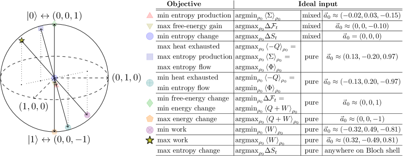
Figure 1: Diversity of ideal inputs for a finite-time qubit-reset process, displayed on and in the Bloch sphere. The states extremizing heat, work, and energy-change all lie on the surface of the Bloch sphere, in the direction of a maximal eigenstate of the corresponding thermodynamic operators. The entire surface of the Bloch sphere maximizes entropy gain. Minimal entropy production and maximal free energy gain are achieved by non-trivial mixed-state inputs. The change in entropy is minimized by the fully-mixed input. Entropy production is maximized by the same pure-state input that maximizes heat exhaustion. The greatest loss of free energy occurs for the same pure-state input that loses the most energy.

X.2 Bounding the behavior of all inputs

Continuing our example of the qubit-reset dynamics, we now leverage our results to identify the extremal thermodynamic behavior that can be attained by any input throughout the process.

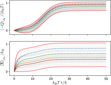
Figure 2: Tracking the behavior of four inputs is enough to bound the behavior of all other inputs to a qubit process. Here we show the the range of expectation values for exhausted heat and entropy production throughout a finite-time qubit-reset process. The expectation values from four random inputs are shown as dashed lines. This allows construction of the thermodynamic operator $\mathcal{Q}$ throughout time. (top) Maximal and minimal heat, corresponding to extremal eigenvalues of $\mathcal{Q}$, shown as thick red solid lines; (bottom) Maximal and minimal entropy production, obtained from gradient descent/ascent, shown as thick red solid lines. These extrema bound the behavior of all other inputs, including the behavior of 100 other random initial conditions shown as thin gray solid lines.

Fig. 2 demonstrates that thermodynamic observations from just four inputs yield the full range of thermodynamic behavior from any input. For example, the min and max expected work at any time $t\in[0,\tau]$, obtainable from alternative inputs, is determined by the expected-work operator at that time. The expected-work operator at any time is constructed from the expected work performed on each of the four test inputs up to that time. Determining the ranges of work, energy change, and heat thus reduces to determining eigenvalue ranges of the respective Hermitian operators.

Determining the range of entropy production throughout the process is somewhat more complicated, although it still only requires the data from four test inputs. Notably, in the bottom panel of Fig. 2, we find the states of minimal and maximal entropy production at times before the state is fully reset. This employs the gradient-descent algorithm developed in Sec. VIII.1.

XI Example 2: Extracting work from a spatially extended state

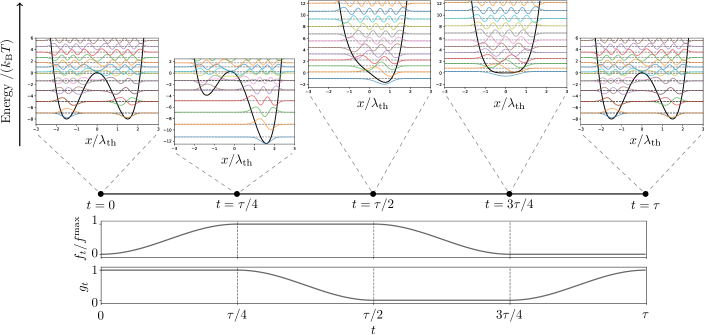
Figure 3: Control protocol to extract work from the nonequilibrium state of a particle on the right-hand side of a double-well potential, via a time-varying one-dimensional potential-energy landscape in the quantum regime. Middle and bottom panel show the protocol for tilting the potential and lowering the energetic barrier, respectively. The top panels show the potential-energy landscape at five representative times along the protocol, staggered so that they share the same energy axis. We show a spatial representation of the lowest-lying energy eigenstates in these potentials, at the height of their respective energy eigenvalues.

Let us now turn to the analysis of an infinite-dimensional quantum system: a charged particle in a time-dependent potential, in the presence of electromagnetic background radiation. This can be interpreted as an idealized model of a double quantum dot in the single-particle zero-current regime. In this example, we use time-dependent Lindbladian dynamics, with a time-modulated double-well of potential energy across one spatial dimension. The protocol is capable of extracting work from some states that are initially localized in the right well. We consider the ideal input (for the task of work extraction), and how it compares to the performance of other inputs, within the Hilbert space spanned by the eight lowest lying energy eigenstates of the initial Hamiltonian.

We will quantify work extraction simply as the negative work performed. In principle, this work can be extracted by a more explicit mechanism, like proposed in Ref. [19].

Given any protocol for work extraction, we can construct the expected-work operator to determine its breadth of behavior on all possible inputs. The device will be best at extracting work from the lowest lying eigenstate of the expected-work operator; the corresponding minimal-eigenvalue magnitude reports the maximal possible expected value of extractable work.

In particular, we simulate a work-extraction protocol via the time-dependent system Hamiltonian $H_{t}=\frac{p_{x}^{2}}{2m}+V_{t}$ where $p_{x}=-i\hbar\partial_{x}$ is the momentum operator and $m$ is the mass of the single-particle system. The time-dependent potential-energy landscape is

$$V_{t}=16h_{0}\Bigl{(}\frac{x}{w_{0}}\Bigr{)}^{4}-8h_{0}\Bigl{(}\frac{x}{w_{0}}\Bigr{)}^{2}g_{t}-h_{0}\frac{x}{w_{0}}f_{t}~{},$$ (47)

where $g_{t}$ and $f_{t}$ are non-negative scalar functions of time, with $g_{0}=g_{\tau}=1$ and $f_{0}=f_{\tau}=0$. To enter an interesting thermodynamic regime, we choose the initial energy barrier between the two wells to be $h_{0}=8k_{\text{B}}T$, where $k_{\text{B}}T=1/\beta$ is the thermal energy of the environment. To enter an interesting quantum regime, we choose the initial separation between the bottom of the two wells to be $w_{0}=3\lambda_{\text{th}}$, where $\lambda_{\text{th}}=\hbar\sqrt{2\pi\beta/m}$ is the thermal de Broglie wavelength. To induce nonequilibrium quantum dynamics, we choose a sufficiently fast protocol.

As depicted in Fig. 3, $g_{t}$ controls the height of the barrier while $f_{t}$ controls the tilt of the energetic landscape throughout the protocol. For a semiconductor-based double quantum dot, the barrier height and tilt could plausibly be modulated by applied voltages, gating the barrier and the bias across the device, respectively [20]. Note that the protocol is cyclic, since the initial and final Hamiltonian are both the same symmetric double-well potential. During the protocol, the potential is tilted to the right, the barrier is lowered, the potential is untilted, and the barrier is then reintroduced, in that order.  The exact form of the control protocol is given in App. J.

The system is coupled to a thermal environment throughout the protocol. For our demonstration, we model the excitation and relaxation dynamics when the system interacts with the photon bath of an ideal blackbody at temperature $T$. The resulting dynamics of the system during the protocol can be described by a Lindblad master equation $\dot{\rho}_{t}=\mathcal{L}_{t}(\rho_{t})$, given explicitly in App. J, which satisfies detailed balance in bath-mediated transitions between instantaneous energy eigenstates.

We simulate a regime that could plausibly be demonstrated in a room-temperature laboratory experiment using a nanofabricated device. The resulting dynamics exhibits a separation of timescales, where the relaxation dynamics are much slower than the timescale of coherent oscillations between energy eigenstates. (Dissipative transitions occur approximately only once per 100 million periods of phase oscillation between energy levels with a $k_{\text{B}}T$ energy spacing.) We develop special methods to efficiently simulate the quantum dynamics (App. J.1) and thermodynamics (App. J.2) over the extended duration $\tau=4\times 10^{9}\beta\hbar\approx 100\,\mu$s of the nonequilibrium protocol.

Which initial state yields the most extracted work given this protocol? To determine this, we construct the expected-work operator $\mathcal{W}$ acting on the Hilbert space spanned by the eight lowest lying initial energy eigenstates, via simulating the behavior of 64 random linearly independent initial states within this subspace. In our simulations, these initially restricted states evolve through the Hilbert space spanned by the twenty lowest lying instantaneous energy eigenstates throughout the protocol.

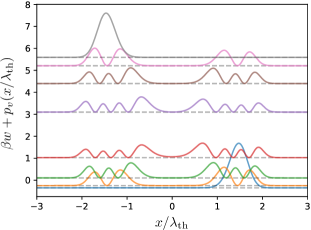
Figure 4: Spatial probability density $p_{v}(x/\lambda_{\text{th}})=\lim_{\delta x\to 0}\frac{\lambda_{\text{th}}}{\delta x}\,|\langle x,\,x+\delta x|v\rangle|^{2}$ for the eigenstates $\ket{v}$ of the expected-work operator $\mathcal{W}$, offset by the corresponding work eigenvalue $w$, such that $\mathcal{W}\ket{v}=w\ket{v}$.

Fig. 4 depicts the eigenvalues and eigenstates of the expected-work operator, via their spatial probability density functions. Two eigenmodes of the expected-work operator allow for work extraction, while the other six modes require a work investment. As one might expect, the ideal initial state leading to maximal work extraction is initially localized in the right well. This state is approximately formed from equal parts of the two lowest lying energy eigenstates. It is also intuitive that the worst input begins purely in the left well.

The remaining six non-extremal eigenstates of the expected-work operator are less immediately intuitive—yet they yield interesting insights once properly understood. As suggested by the spatial probability density functions in Fig. 4, each work-eigenstate is approximately a linear combination of up-to-two energy eigenstates (although in detail they contain contributions from all). Some investigation revealed that each work eigenstate roughly corresponds to a relative phase combination of energy eigenstates that leaves the particle either mostly in the right well (for small eigenwork) or mostly in the left well (for large eigenwork) during the first half of the protocol. Fig. 4 displays some kind of symmetry in the vertical spacing of work eigenvalues that could likely be related to fluctuation relations, although that investigation remains an open opportunity.

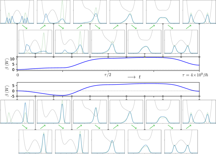
Figure 5: Bottom panels: Snapshots of spatial evolution of the ideal input to the work-extraction protocol, along with the resulting trajectory of expected work. Upper panels: Snapshots of spatial evolution of a random input to the protocol, along with the resulting trajectory of expected work. Top and bottom panels show spatial probability density of the state in thick solid blue, compared to the probability density for the instantaneous equilibrium state in thin dashed green; the instantaneous potential-energy landscape, which starts and ends as a symmetric double well, is shown in thin solid gray. The two long middle panels show the time evolution of the expected work from each of these two initial states.

The ideal input to this particular work-extraction protocol yields approximately $0.3472\,k_{\text{B}}T$ of extracted work ($\braket{W}=-0.3472\,k_{\text{B}}T$), which is about half of the nonequilibrium addition to free energy ($\approx k_{\text{B}}T\ln 2$) available from that initial state. This work-extraction value was initially found via the minimal eigenvalue of the expected-work operator, and subsequently verified via direct simulation of this ideal input. The spatial evolution of this ideal state, and the corresponding work trajectory are shown in the bottom half of Fig. 5. There it is apparent that the ideal state remains on the right well for the first half of the work-extraction protocol.

For comparison, the top half of Fig. 5 shows the spatial evolution and corresponding work trajectory of a random input (in particular, we chose one of the initial energy eigenstates). No work is extracted when operating on this state; rather, about $4.138\,k_{\text{B}}T$ of work must be expended in the process. We verified that this same work value is obtained (through ten significant digits) both from the full simulation and from the simple algebraic employment of the expected-work operator : $\text{tr}(\rho_{0}\mathcal{W})\approx 4.138\,k_{\text{B}}T$. The series of panels in the top half of Fig. 5 reveals the work penalty for populating the left well during the first half of the protocol. The chronologically second snapshot reveals a slow local equilibration within each well. Subsequent snapshots reveal an even slower tendency towards global equilibration throughout the protocol.

As anticipated by the general theory, the initial state leading to maximal work extraction is a pure state. In this case, this state is close to, but distinct from, the input leading to minimal entropy production—the latter of which is a non-pure mixed state. As a final note, we emphasize that we’ve been able to identify the ideal input within the initial low-energy subspace, although the evolving states were not limited to this subspace during their natural dynamics.

XII Conclusion

We have determined the ideal inputs that minimize or maximize various thermodynamic quantities for any fixed process that transforms a physical system in finite time. Many of these optimal inputs turn out to be pure states corresponding to eigenstates of Hermitian thermodynamic operators. We showed how to reconstruct these operators via observed behavior from a finite number of experimentally accessible input states. Another class of thermodynamic quantities, based on entropies, have mixed-state minimizers but pure-state maximizers. The Hermitian thermodynamic operators determine these ideal states too. Our examples illustrate the incompatibility of common objectives: The ‘ideal’ input depends on whether one intends to minimize heat, minimize entropy production, maximize free-energy gain, maximize work extraction, etc.

This investigation of ideal initial states complements the centuries-old tradition of rather seeking ideal protocols with an assumed initial state. Whether or not a protocol is ideal, our results highlight the initial-state dependence of a device’s performance across thermodynamic metrics, and expose the breadth of its possible behavior. While we emphasized thermodynamics, the results of this paper extend easily to other domains—where the ideal inputs, as judged by some other criteria, like maximizing the yield of a desired output state [21], will be obtained from the linear operators induced by those criteria.

XIII Acknowledgements

AK thanks Sosuke Ito for support. This work is supported by the Singapore Ministry of Education Tier 1 Grants RG146/20, grant no. FQXi-RFP-IPW-1903 (‘Are quantum agents more energetically efficient at making predictions?’) from the Foundational Questions Institute and Fetzer Franklin Fund (a donor-advised fund of Silicon Valley Community Foundation), the National Research Foundation, Singapore, and Agency for Science, Technology and Research (A*STAR) under its QEP2.0 programme (NRF2021-QEP2-02-P06) and the Singapore Ministry of Education Tier 2 Grant MOE-T2EP50221-0005. This project was partly made possible through the support of Grant 62417 from the John Templeton Foundation. The opinions expressed in this publication are those of the authors and do not necessarily reflect the views of the John Templeton Foundation.

Appendix A Existence of thermodynamic operators

Type-I expectation values—for expected work, heat, entropy flow, etc.—are linear functionals of the initial state, since they can all be written as

$$\braket{X}_{\rho_{0}}=\text{tr}[\Xi_{X}(\rho_{0})]~{},$$ (48)

where $\Xi_{X}$ is a linear superoperator acting on the initial density matrix of the system. $\text{tr}[\Xi_{X}(\cdot)]$ is a linear functional since $\Xi_{X}$ and the trace operation are both linear, and the trace returns a scalar value. The superoperator $\Xi_{X}$ is however relatively unwieldy, since it acts on the $d^{2}$ dimensional vector space spanned by density matrices that in turn act on a $d$-dimensional vector space $\mathcal{V}$. The following theorem shows that the same linear functional can be represented via the lower-dimensional operator $\mathcal{X}$ acting on $\mathcal{V}$. This assures the existence of our thermodynamic operators.

Theorem 6.

For any linear functional $\ell$ acting on a finite $d^{2}$-dimensional vector space $\mathcal{V}_{\text{big}}$ of linear operators, which in turn operate on a $d$-dimensional vector space $\mathcal{V}_{\text{small}}$, there exists a linear operator $\mathcal{X}$ acting on $\mathcal{V}_{\text{small}}$ such that

$$\ell(\cdot)=\text{tr}(\mathcal{X}\,\,\cdot\,)~{}.$$ (49)

Proof.

There are only $d^{2}$ linearly independent linear functionals acting on the $d^{2}$-dimensional vector space $\mathcal{V}_{\text{big}}$. Let $K=\{\ket{k}\}_{k=1}^{d}$ be an arbitrary orthonormal basis for $\mathcal{V}_{\text{small}}$, with $\bra{k}=\ket{k}^{\dagger}$. Note that the $d^{2}$ linearly independent linear functionals $\{\text{tr}(\,\ket{j}\bra{k}\,\cdot\,)\}_{\ket{j},\ket{k}\in K}$ form a complete basis for the dual space of $\mathcal{V}_{\text{big}}$. An arbitrary linear functional acting on $\mathcal{V}_{\text{big}}$ can thus be written as a linear combination of these basis functionals:

$$\ell(\cdot)=\sum_{j,k}x_{j,k}\text{tr}(\,\ket{j}\bra{k}\,\cdot\,)=\text{tr}(\mathcal{X}\,\,\cdot\,)$$ (50)

where $\mathcal{X}=\sum_{j,k}x_{j,k}\ket{j}\bra{k}$ and $x_{j,k}=\ell(\ket{k}\bra{j})$. ∎

Hence, for type-I expectation values:

$$\braket{X}_{\rho_{0}}=\text{tr}[\Xi_{X}(\rho_{0})]=\text{tr}(\rho_{0}\mathcal{X})~{}.$$ (51)

Whenever the random variable $X$ is real-valued, its expectation value must also be real valued, and so $\mathcal{X}$ is guaranteed to be Hermitian (see Thm. 2.4.3 of Hassani [6]).

Sometimes the linear superoperator $\Xi_{X}$ can appear very complicated; but only its existence matters to guarantee the existence of the simpler operator $\mathcal{X}$. For example, entropy flow can generically be written as

$$\braket{\Phi}_{\rho_{0}} =-k_{\text{B}}\int_{0}^{\tau}\text{tr}\bigl{(}\dot{\rho}_{t}^{\text{env}}\ln\bm{\pi}_{t}^{\text{env}}\bigr{)}\,dt~{},$$

where $\bm{\pi}_{t}^{\text{env}}$ is assumed to be independent of $\rho_{0}$. If we write out $\dot{\rho}_{t}^{\text{env}}$ more explicitly, we find that

$$\braket{\Phi}_{\rho_{0}} =-k_{\text{B}}\int_{0}^{\tau}\text{tr}\bigl{(}\dot{\rho}_{t}^{\text{env}}\ln\bm{\pi}_{t}^{\text{env}}\bigr{)}\,dt$$

$$=-k_{\text{B}}\int_{0}^{\tau}\text{tr}\bigl{[}(\tfrac{d}{dt}\rho_{t}^{\text{env}})\ln\bm{\pi}_{t}^{\text{env}}\bigr{]}\,dt$$ (52)

$$=-k_{\text{B}}\int_{0}^{\tau}\text{tr}\Bigl{\{}\bigl{[}\tfrac{d}{dt}\text{tr}_{\text{sys}}(U_{t}\rho_{0}\otimes\rho_{0}^{\text{env}}U_{t}^{\dagger})\bigr{]}\ln\bm{\pi}_{t}^{\text{env}}\Bigr{\}}\,dt$$ (53)

$$=\text{tr}\Bigl{\{}-k_{\text{B}}\int_{0}^{\tau}\bigl{[}\tfrac{d}{dt}\text{tr}_{\text{sys}}(U_{t}\rho_{0}\otimes\rho_{0}^{\text{env}}U_{t}^{\dagger})\bigr{]}\ln\bm{\pi}_{t}^{\text{env}}\,dt\Bigr{\}}~{}.$$ (54)

Hence, we’ve found the relevant linear superoperator $\Xi_{\Phi}(\cdot)=-k_{\text{B}}\int_{0}^{\tau}\bigl{[}\tfrac{d}{dt}\text{tr}_{\text{sys}}(U_{t}\,\cdot\,\otimes\rho_{0}^{\text{env}}U_{t}^{\dagger})\bigr{]}\ln\bm{\pi}_{t}^{\text{env}}\,dt$, which is somewhat complicated. No matter: Its mere existence proves the existence of some simpler linear operator $\bm{\Phi}$ such that $\braket{\Phi}_{\rho_{0}}=\text{tr}(\rho_{0}\bm{\Phi})$ for any initial state $\rho_{0}$.

A similar procedure reveals the existence of the relevant linear superoperator $\Xi(\cdot)$ for work and heat, which in turn implies the existence of the simpler expected-work operator $\mathcal{W}$ and expected-heat operator $\mathcal{Q}$.

Expanding the expression for expected work, we find

$$\braket{W}_{\rho_{0}} =\int_{0}^{\tau}\text{tr}\bigl{(}\rho_{t}\dot{H}_{t}\bigr{)}\,dt$$

$$=\text{tr}\Bigl{[}\int_{0}^{\tau}\text{tr}_{\text{env}}(U_{t}\rho_{0}\otimes\rho_{0}^{\text{env}}U_{t}^{\dagger})\dot{H}_{t}\,dt\Bigr{]}~{}.$$ (55)

Hence, the linear superoperator $\Xi_{W}(\cdot)=\int_{0}^{\tau}\text{tr}_{\text{env}}(U_{t}\,\cdot\,\otimes\rho_{0}^{\text{env}}U_{t}^{\dagger})\dot{H}_{t}\,dt$ implies the existence of the simpler expected-work operator $\mathcal{W}$.

Expanding the expression for expected heat, we find

$$\braket{Q}_{\rho_{0}} =\int_{0}^{\tau}\text{tr}\bigl{(}\dot{\rho}_{t}H_{t}\bigr{)}\,dt$$

$$=\text{tr}\Bigl{\{}\int_{0}^{\tau}\bigl{[}\tfrac{d}{dt}\text{tr}_{\text{env}}(U_{t}\rho_{0}\otimes\rho_{0}^{\text{env}}U_{t}^{\dagger})\bigr{]}H_{t}\,dt\Bigr{\}}~{}.$$ (56)

Hence, the linear superoperator $\Xi_{Q}(\cdot)=\int_{0}^{\tau}\bigl{[}\tfrac{d}{dt}\text{tr}_{\text{env}}(U_{t}\,\cdot\,\otimes\rho_{0}^{\text{env}}U_{t}^{\dagger})\bigr{]}H_{t}\,dt$ implies the existence of the simpler expected-heat operator $\mathcal{Q}$.

Appendix B Thermodynamic operators characterize any measurement scheme

Invasive measurements change not only the probability distribution for work, but also the expected value for work under the prescribed measurement protocol [7]. Our framework applies just as well to these alternative protocols with measurement interventions. For example, let us briefly describe how our framework applies to the famous two-point-measurement (TPM) scheme for driven isolated quantum systems, which projects the state onto the instantaneous energy eigenbasis at both the beginning and end of the protocol [8].

If we are interested in the TPM scheme for a driven isolated quantum system, the relevant expected-TPM-work operator is

$$\mathcal{W}_{\text{TPM}}=\sum_{\ket{E}\in V_{H}}\ket{E}\!\bra{E}\sum_{\ket{E^{\prime}}\in V_{H^{\prime}}}(E^{\prime}-E)\bigl{|}\braket{E^{\prime}}{U_{\tau}}{E}\bigr{|}^{2}~{},$$ (57)

where $H$ and $H^{\prime}$ are the initial and final Hamiltonians for the system respectively, and $U_{\tau}$ unitarily evolves the system between the two projective measurements. In the TPM scheme, the system transitions from initial energy eigenstate $\ket{E}$ to final energy eigenstate $\ket{E^{\prime}}$ with probability $\braket{E}{\rho_{0}}{E}\bigl{|}\braket{E^{\prime}}{U_{\tau}}{E}\bigr{|}^{2}$, resulting in a TPM work value of $E^{\prime}-E$. It is easy to verify that

$$\braket{W_{\text{TPM}}}_{\rho_{0}}=\sum_{w}w\Pr(W_{\text{TPM}}=w)=\text{tr}(\rho_{0}\mathcal{W}_{\text{TPM}})~{},$$ (58)

where $W_{\text{TPM}}$ is the random variable for the TPM work outcome, and the sum runs over all $w\in\{E^{\prime}-E:E\in\Lambda_{H},E^{\prime}\in\Lambda_{H^{\prime}}\}$.

Ref. [7] shows that $\mathcal{W}\neq\mathcal{W}_{\text{TPM}}$. Invasive measurements can change the expectation value for work (and indeed for other thermodynamic variables too).

If desired, our framework can be employed to find the ideal inputs leading to minimal or maximal TPM work, from the minimal and maximal eigenstates of $\mathcal{W}_{\text{TPM}}$. Indeed, for any measurement scheme—including also the one-time-measurement scheme [9, 10, 11] or any other—thermodynamic operators can be constructed, and our framework can be applied to identify both the breadth of behavior and the ideal inputs within the scheme.

Appendix C Expectation-value invariance to subensemble decomposition

Our contributions in the main text exclusively involve expectation values, so are invariant to density-matrix decompositions. Here we show this invariance explicitly. As an added benefit, it can be useful to see how the quantum random variables induced by a subensemble decomposition relate to and generalize their classical counterparts.

In the classical case, fluctuations are primarily due to subjective uncertainty about which state the environment is in (although uncertainty of the system state also plays a role). Since quantum results should include classical results as a special case, we must also consider the role of subjective uncertainty in the quantum case. In general, this can be addressed via a probability distribution over (possibly nonorthogonal) subensembles of the joint system–environment supersystem [12].

There are many ways to decompose the initial joint density matrix of the system–environment supersystem. In fact for a non-pure mixed state $\rho_{0}^{\text{tot}}$, there are infinitely many pairs $\bigl{(}(p_{n})_{n},(\sigma_{n})_{n}\bigr{)}$ of probability distributions $(p_{n})_{n}$ over constituent density matrices $(\sigma_{n})_{n}$, for which $\rho_{0}^{\text{tot}}=\sum_{n}\sigma_{n}p_{n}$. Each of these decompositions can represent a physically relevant preparation of the supersystem [12, 22].

Each subensemble decomposition $\bigl{(}(p_{n})_{n},(\sigma_{n})_{n}\bigr{)}$ induces a random variable $X\bigl{(}(p_{n})_{n},(\sigma_{n})_{n}\bigr{)}$.  With probability $p_{n}$, the subensemble $\sigma_{n}$ will be realized, in which case the random variable $X$ takes on the value $x(\sigma_{n})$. When the thermodynamic quantity is a linear functional of the initial state—as is the case for work, heat, entropy flow, etc.—it’s easy to see that

$$\Bigl{\langle}X\bigl{(}(p_{n})_{n},(\sigma_{n})_{n}\bigr{)}\Bigr{\rangle}_{n}=\sum_{n}x(\sigma_{n})p_{n}=x\Bigl{(}\sum_{n}\sigma_{n}p_{n}\Bigr{)}=x(\rho_{0}^{\text{tot}})~{},$$ (59)

independent of the decomposition. In the main text, we always consider $\rho_{0}^{\text{tot}}=\rho_{0}\otimes\rho_{0}^{\text{env}}$ for a fixed initial state of the environment $\rho_{0}^{\text{env}}$. For these thermodynamic linear functionals, we thus use the shorthand notation

$$\braket{X}_{\rho_{0}}=x(\rho_{0}\otimes\rho_{0}^{\text{env}})~{}.$$ (60)

As a consequence, the expectation value $\braket{X}_{\rho_{0}}$ and thermodynamic operator $\mathcal{X}$ are both invariant to subensemble decompositions.

Let’s take thermodynamic work (without measurement interventions) as an example. From Eq. (55), we see that work can be quantified for any initial joint state $\sigma$ of the supersystem via

$$w(\sigma)=\text{tr}\Bigl{[}\int_{0}^{\tau}\text{tr}_{\text{env}}(U_{t}\sigma U_{t}^{\dagger})\dot{H}_{t}\,dt\Bigr{]}~{}.$$ (61)

If the system and environment are unmeasured, then it is natural for eigenvalues of the uncorrelated density matrix to represent subjective uncertainty. We can thus take $\bigl{(}(p_{n})_{n},\ket{n}\!\bra{n}\bigr{)}$ as our subensemble decomposition, where $\ket{n}$ is an eigenstate of $\rho_{0}^{\text{tot}}$. In this case, work will be a random variable $W$ which takes on the value $w^{(n)}=w\bigl{(}\ket{n}\!\bra{n}\bigr{)}$ with probability $\sum_{m}p_{m}\delta_{w^{(m)},w^{(n)}}$. We can then write

$$\braket{W}_{\rho_{0}}=\sum_{n}w^{(n)}p_{n}=w(\rho_{0}\otimes\rho_{0}^{\text{env}})=\text{tr}(\rho_{0}\mathcal{W})~{}.$$ (62)

We see that the expectation value and the thermodynamic operator are both independent of the chosen subensemble decomposition.

Appendix D Operator expressions for type-II expectation values

The expectation values of entropy production, the reduction in nonequilibrium free energy, and the change in von Neumann entropy can all be written as:

$$f_{\rho_{0}}^{(\mathcal{X})} =\text{tr}(\rho_{0}\mathcal{X})+S(\rho_{\tau})-S(\rho_{0})$$ (63)

$$=\text{tr}(\rho_{0}\ln\rho_{0})-\text{tr}(\rho_{0}\ln e^{-\mathcal{X}})+S(\rho_{\tau})$$ (64)

$$=\text{tr}(\rho_{0}\ln\rho_{0})-\text{tr}\{\rho_{0}\ln[e^{-\mathcal{X}}/\text{tr}(e^{-\mathcal{X}})]\}-\ln[\text{tr}(e^{-\mathcal{X}})]+S(\rho_{\tau})$$ (65)

$$=\text{D}[\rho_{0}\|\omega]-\ln[\text{tr}(e^{-\mathcal{X}})]+S(\rho_{\tau})~{},$$ (66)

where $\omega\coloneqq e^{-\mathcal{X}}/\text{tr}(e^{-\mathcal{X}})$.

For reliable reset processes, for which $\rho_{\tau}\approx r_{\tau}$ is very nearly independent of the input, it is clear that $\omega$ minimizes $f_{\rho_{0}}^{(\mathcal{X})}$, where it takes on the minimal value $f_{\omega}^{(\mathcal{X})}=S(r_{\tau})-\ln[\text{tr}(e^{-\mathcal{X}})]$.

Ref. [4] pointed out that entropy production can be written in this form. Here we notice that this type of relation applies also to a larger family of thermodynamic quantities.

Appendix E Generalized Gell-Mann matrices as a standard operator basis

For concreteness, we will describe an operator basis that can be used in any finite dimension $d$.

Let $\bigl{\{}\ket{1},\dots,\ket{d}\bigr{\}}$ be an orthonormal basis for the $d$-dimensional Hilbert space of our system under study. We can then construct the generalized Gell-Mann matrices to complete a matrix basis for density matrices acting on this Hilbert space.

Let $n\in\mathbb{R}$ be any convenient constant. $\vec{\Gamma}$ will contain $d-1$ diagonal matrices

$$n\Bigl{(}\tfrac{2}{\ell^{2}+\ell}\Bigr{)}^{\!1/2}\,\Bigl{[}\Bigl{(}\sum_{j=1}^{\ell}\ket{j}\bra{j}\Bigr{)}-\ell\ket{\ell+1}\bra{\ell+1}\Bigr{]}~{},$$ (67)

with $\ell\in\{1,\dots,d-1\}$. It will contain $(d^{2}-d)/2$ distinct non-diagonal symmetric matrices

$$n\bigl{(}\ket{k}\bra{j}+\ket{j}\bra{k}\bigr{)}~{},$$ (68)

with $1\leq j<k\leq d$. It will also contain $(d^{2}-d)/2$ distinct antisymmetric matrices

$$in\bigl{(}\ket{k}\bra{j}-\ket{j}\bra{k}\bigr{)}~{},$$ (69)

with $1\leq j<k\leq d$. The ordering of these $d^{2}-1$ matrices is arbitrary.

Notice that these operators are traceless and satisfy $\text{tr}(\Gamma_{m}\Gamma_{n})=2n^{2}\delta_{m,n}$. Hence, $\eta=2n^{2}$. If we choose $n=\sqrt{\tfrac{d-1}{2d}}$, then $\eta=\tfrac{d-1}{d}$, pure states will always have a generalized Bloch vector of unit length, and the generalized Bloch vector will reduce to the standard Bloch vector in $d=2$.

Appendix F Composite operator bases

Suppose we have normalized Hermitian operator bases, ($I_{d}/d,\,\vec{\Gamma}$) for a $d$-dimensional subsystem, and ($I_{d^{\prime}}/d^{\prime},\,\vec{\Gamma^{\prime}}$) for a $d^{\prime}$-dimensional subsystem. The operator bases satisfy

$$\text{tr}(\Gamma_{n})=0\quad\text{and}\quad\text{tr}(\Gamma_{m}\Gamma_{n})=\eta\delta_{m,n}$$ (70)

and

$$\text{tr}(\Gamma_{n}^{\prime})=0\quad\text{and}\quad\text{tr}(\Gamma_{m}^{\prime}\Gamma_{n}^{\prime})=\eta^{\prime}\delta_{m,n}~{}.$$ (71)

We can then construct a normalized Hermitian basis for operators acting on the composite $d^{\prime\prime}$-dimensional Hilbert space, where $d^{\prime\prime}=dd^{\prime}$: The new operator basis, ($I_{d^{\prime\prime}}/d^{\prime\prime},\,\vec{\Gamma^{\prime\prime}}$) satisfies

$$\text{tr}(\Gamma_{n}^{\prime\prime})=0\quad\text{and}\quad\text{tr}(\Gamma_{m}^{\prime\prime}\Gamma_{n}^{\prime\prime})=\eta^{\prime\prime}\delta_{m,n}~{},$$ (72)

where the new composite operator basis contains

$$\vec{\Gamma^{\prime\prime}}=\Bigl{(}\sqrt{\tfrac{\eta^{\prime\prime}}{\eta^{\prime}d}}I_{d}\otimes\vec{\Gamma^{\prime}},\,\,\,\sqrt{\tfrac{\eta^{\prime\prime}}{\eta d^{\prime}}}\vec{\Gamma^{\prime\prime}}\otimes I_{d^{\prime}},\,\,\,\sqrt{\tfrac{\eta^{\prime\prime}}{\eta\eta^{\prime}}}\vec{\Gamma}\otimes\vec{\Gamma^{\prime}}\Bigr{)}~{}.$$ (73)

Eq. (72) can be verified via the identities $(A\otimes B)(C\otimes D)=(AC)\otimes(BD)$ and $\text{tr}(A\otimes B)=\text{tr}(A)\text{tr}(B)$.

This allows us, for example, to build up a normalized Hermitian operator basis for

• many qubits, using tensor products of the local Pauli operators, or

• a qubit and qutrit, using tensor products of their local Pauli and Gell-Mann operators,

• etc.

Appendix G Existence of, and expression for, the entropy-flow vector

Leveraging the decomposition of the system state in terms of its generalized Bloch vector, $\rho_{t}=I/d+\vec{b}_{t}\cdot\vec{\Gamma}$, we can expand the general expression for entropy flow given in Ref. [3] and discussed in the main text, to express entropy flow in terms of the entropy-flow vector and initial Bloch vector:

$$\braket{\Phi}_{\rho_{0}} =-k_{\text{B}}\int_{0}^{\tau}\text{tr}\bigl{(}\dot{\rho}_{t}^{\text{env}}\ln\bm{\pi}_{t}^{\text{env}}\bigr{)}\,dt$$ (74)

$$=-k_{\text{B}}\int_{0}^{\tau}\text{tr}\biggl{\{}\Bigl{[}\tfrac{d}{dt}\text{tr}_{\text{sys}}\bigl{(}U_{0:t}\rho_{0}\otimes\rho_{0}^{\text{env}}U_{0:t}^{\dagger}\bigr{)}\Bigr{]}\ln\bm{\pi}_{t}^{\text{env}}\biggr{\}}\,dt$$ (75)

$$=-k_{\text{B}}\int_{0}^{\tau}\text{tr}\biggl{\{}\Bigl{[}\tfrac{d}{dt}\text{tr}_{\text{sys}}\bigl{(}U_{0:t}(I/d+\vec{b}_{0}\cdot\vec{\Gamma})\otimes\rho_{0}^{\text{env}}U_{0:t}^{\dagger}\bigr{)}\Bigr{]}\ln\bm{\pi}_{t}^{\text{env}}\biggr{\}}\,dt$$ (76)

$$=\underbrace{-k_{\text{B}}\int_{0}^{\tau}\text{tr}\biggl{\{}\Bigl{[}\tfrac{d}{dt}\text{tr}_{\text{sys}}\bigl{(}U_{0:t}I/d\otimes\rho_{0}^{\text{env}}U_{0:t}^{\dagger}\bigr{)}\Bigr{]}\ln\bm{\pi}_{t}^{\text{env}}\biggr{\}}\,dt}_{=\braket{\Phi}_{I/d}}+\vec{b}_{0}\cdot\Biggl{(}\underbrace{-k_{\text{B}}\int_{0}^{\tau}\text{tr}\biggl{\{}\Bigl{[}\tfrac{d}{dt}\text{tr}_{\text{sys}}\bigl{(}U_{0:t}\vec{\Gamma}\otimes\rho_{0}^{\text{env}}U_{0:t}^{\dagger}\bigr{)}\Bigr{]}\ln\bm{\pi}_{t}^{\text{env}}\biggr{\}}\,dt}_{\eqqcolon\vec{\varphi}}\Biggr{)}$$ (77)

$$=\braket{\Phi}_{I/d}+\vec{b}_{0}\cdot\vec{\varphi}~{}.$$ (78)

Other thermodynamic quantities can be decomposed similarly.

Appendix H Expression for the second derivative of von Neumann entropy

The second derivative of von Neumann entropy, with respect to the elements of the Bloch vector of the quantum state, can be calculated via the spectral decomposition of the quantum state $\tilde{\rho}(\vec{b})=\sum_{k}\lambda_{k}\ket{k}\bra{k}$ and its logarithm $\ln\tilde{\rho}(\vec{b})=\sum_{k}\ln(\lambda_{k})\ket{k}\bra{k}$. Assuming non-degeneracy of the eigenvalues, we find

$$\partial_{b_{m}}\partial_{b_{n}}S[\tilde{\rho}(\vec{b})] =-\partial_{b_{m}}\text{tr}\bigl{[}\Gamma_{n}\ln\tilde{\rho}(\vec{b})\bigr{]}$$ (79)

$$=-\text{tr}\bigl{[}\Gamma_{n}\,\partial_{b_{m}}\ln\tilde{\rho}(\vec{b})\bigr{]}~{},$$ (80)

where

$$\partial_{b_{m}}\ln\tilde{\rho}(\vec{b}) =\sum_{k}\biggl{\{}\frac{1}{\lambda_{k}}\underbrace{(\partial_{b_{m}}\lambda_{k})}_{\braket{k}{\Gamma_{m}}{k}}\ket{k}\bra{k}+\ln(\lambda_{k})\Bigl{[}\!\!\!\!\underbrace{\bigl{(}\partial_{b_{m}}\ket{k}\bigr{)}}_{\sum_{\ell\neq k}\frac{\braket{\ell}{\Gamma_{m}}{k}}{\lambda_{k}-\lambda_{\ell}}\ket{\ell}}\!\!\!\!\!\!\bra{k}\,+\,\ket{k}\!\!\!\!\!\!\underbrace{\bigl{(}\partial_{b_{m}}\bra{k}\bigr{)}}_{\sum_{\ell\neq k}\frac{\braket{k}{\Gamma_{m}}{\ell}}{\lambda_{k}-\lambda_{\ell}}\bra{\ell}}\!\!\!\!\Bigr{]}\biggr{\}}~{}.$$ (81)

Hence,

$$\partial_{b_{m}}\partial_{b_{n}}S[\tilde{\rho}(\vec{b})] =\biggl{(}\sum_{k}\tfrac{1}{\lambda_{k}}\braket{k}{\Gamma_{n}}{k}\braket{k}{\Gamma_{m}}{k}\biggr{)}+\biggl{(}\sum_{k,\ell\atop\ell\neq k}\frac{\ln\lambda_{k}}{\lambda_{k}-\lambda_{\ell}}\braket{k}{\Gamma_{n}}{\ell}\braket{\ell}{\Gamma_{m}}{k}\biggr{)}+\biggl{(}\sum_{k,\ell\atop\ell\neq k}\frac{\ln\lambda_{k}}{\lambda_{k}-\lambda_{\ell}}\braket{\ell}{\Gamma_{n}}{k}\braket{k}{\Gamma_{m}}{\ell}\biggr{)}~{}.$$ (82)

Upon swapping the name of the indices in the last of the three terms on the right-hand side of Eq. (82), we find

$$\sum_{k,\ell\atop\ell\neq k}\frac{\ln\lambda_{k}}{\lambda_{k}-\lambda_{\ell}}\braket{\ell}{\Gamma_{n}}{k}\braket{k}{\Gamma_{m}}{\ell} =\sum_{\ell,k\atop k\neq\ell}\frac{\ln\lambda_{\ell}}{\lambda_{\ell}-\lambda_{k}}\braket{k}{\Gamma_{n}}{\ell}\braket{\ell}{\Gamma_{m}}{k}$$ (83)

$$=\sum_{k,\ell\atop\ell\neq k}\frac{-\ln\lambda_{\ell}}{\lambda_{k}-\lambda_{\ell}}\braket{k}{\Gamma_{n}}{\ell}\braket{\ell}{\Gamma_{m}}{k}~{}.$$ (84)

Noting that $\lim_{b\to a}\frac{\ln a-\ln b}{a-b}=1/a$, we can thus combine all three terms on the right-hand side of Eq. (82) to find

$$\partial_{b_{m}}\partial_{b_{n}}S[\tilde{\rho}(\vec{b})] =-\sum_{k,\ell}\phi(\lambda_{k},\lambda_{\ell})\braket{k}{\Gamma_{n}}{\ell}\braket{\ell}{\Gamma_{m}}{k}~{},$$ (85)

where we defined $\phi(a,b)\coloneqq\frac{\ln a-\ln b}{a-b}$ (with $\phi(a,a)=1/a$ by continuity). Note that $\phi(a,b)$ is the reciprocal of the logarithmic mean of the eigenvalues $a$ and $b$.

Similarly, using the spectral decomposition of $\tilde{\rho}^{\prime}(\vec{b})=\sum_{k}\lambda_{k}^{\prime}\ket{k^{\prime}}\bra{k^{\prime}}$, we find

$$\partial_{b_{m}}\partial_{b_{n}}S[\tilde{\rho}^{\prime}(\vec{b})] =-\sum_{k,\ell}\phi(\lambda_{k}^{\prime},\lambda_{\ell}^{\prime})\braket{k^{\prime}}{\Gamma_{n}^{\prime}}{\ell^{\prime}}\braket{\ell^{\prime}}{\Gamma_{m}^{\prime}}{k^{\prime}}~{}.$$ (86)

Appendix I Dynamical equations for a qubit-reset device

Here we review the dynamical equations for a particular device that implements qubit reset, used in our first example: As in Refs. [23, 3], the device works by changing both the energy gap and spatial orientation of the energy eigenstates of the qubit while it is in weak contact with a thermal reservoir at inverse temperature $\beta=1/(k_{\text{B}}T)$. Over the finite-time protocol, from time $0$ through $\tau=50\beta\hbar$, the time-varying Hamiltonian is

$$H_{t}=\frac{E_{t}}{2}\bigl{[}\cos(\theta_{t})\sigma_{z}+\sin(\theta_{t})\sigma_{x}\bigr{]}~{},$$ (87)

with $E_{t}=k_{\text{B}}T[1+49\sin^{2}\bigl{(}\tfrac{\pi t}{100\beta\hbar}\bigr{)}]/5$ and $\theta_{t}=\pi t/(50\beta\hbar)$. While $E_{t}$ quantifies the energy gap between the system’s instantaneous energy eigenstates, $\theta_{t}$ parametrizes the instantaneous orientation of the energy eigenbasis relative to the ‘computational’ $z$-basis. The dynamics are well-described by a time-dependent quantum master equation

$$\dot{\rho}_{t}=\mathcal{L}_{x_{t}}(\rho_{t})=\frac{i}{\hbar}[\rho_{t},H_{x_{t}}] +\frac{cE_{t}}{\hbar}(N_{x_{t}}+1)\mathcal{D}[L_{x_{t}}](\rho_{t})+\frac{cE_{t}}{\hbar}N_{x_{t}}\mathcal{D}[L_{x_{t}}^{\dagger}](\rho_{t})$$ (88)

where $\mathcal{D}[L](\rho)=L\rho L^{\dagger}-\tfrac{1}{2}\{L^{\dagger}L,\rho\}$, $N_{x_{t}}=(e^{\beta E_{t}}-1)^{-1}$, and $c=1/5$ is the coupling strength to the bath. The time-dependent lowering operator can be represented as

$$L_{x_{t}}=\frac{1}{2}\bigl{[}\cos(\theta_{t})\sigma_{x}-i\sigma_{y}-\sin(\theta_{t})\sigma_{z}\bigr{]}$$ (89)

and satisfies the detailed balance condition $[L_{x_{t}},H_{x_{t}}]=E_{t}L_{x_{t}}$  [23, 24]. Transitions thus occur between instantaneous energy eigenstates of the system. In particular, $\mathcal{D}[L_{x_{t}}](\rho_{t})$ takes the excited population and shifts it to the ground state, while $\mathcal{D}[L_{x_{t}}^{\dagger}](\rho_{t})$ takes the ground-state population and shifts it to the excited state. Moreover, the ratio of transition rates between the excited and ground-state populations satisfies detailed balance since $(N_{x_{t}}+1)/N_{x_{t}}=e^{\beta E_{t}}$.

Appendix J Time-dependent double-well dynamics

Here we construct a simple model for the dynamics of a non-relativistic charged particle in a time-dependent double-well of potential energy across one spatial dimension while it is immersed in a bosonic bath at temperature $T$. The protocol is capable of extracting work from some states that are initially localized in the right well.

In particular, we simulate a work-extraction protocol via the time-dependent system Hamiltonian:

$$H_{t}=\frac{p_{x}^{2}}{2m_{q}}+V_{t}$$ (90)

where $p_{x}=-i\hbar\partial_{x}$ is the momentum operator and $m_{q}$ is the mass of the system with charge $q$. The time-dependent potential-energy landscape is

$$V_{t}=16h_{0}\Bigl{(}\frac{x}{w_{0}}\Bigr{)}^{4}-8h_{0}\Bigl{(}\frac{x}{w_{0}}\Bigr{)}^{2}g_{t}-h_{0}\frac{x}{w_{0}}f_{t}~{},$$ (91)

where $g_{t}$ and $f_{t}$ are non-negative scalar functions of time, with $g_{0}=g_{\tau}=1$ and $f_{0}=f_{\tau}=0$. To enter an interesting thermodynamic regime, we choose the initial energy barrier between the two wells to be $h_{0}=8k_{\text{B}}T$, where $k_{\text{B}}T=1/\beta$ is the thermal energy of the environment. To enter an interesting quantum regime, we choose the initial separation between the bottom of the two wells to be $w_{0}=3\lambda_{\text{th}}$, where $\lambda_{\text{th}}=\hbar\sqrt{2\pi\beta/m_{q}}$ is the thermal de Broglie wavelength. To induce nonequilibrium quantum dynamics, we choose a sufficiently fast protocol.

$g_{t}$ controls the height of the barrier while $f_{t}$ controls the tilt of the energetic landscape throughout the protocol. During the protocol, the potential is tilted to the right, the barrier is lowered, the potential is untilted, and the barrier is then reintroduced, in that order. The exact form of the control protocol is given by

$$g_{t}=\begin{cases}1&\text{if }0\leq t<\tau/4\\ \sin^{2}(2\pi t/\tau)&\text{if }\tau/4\leq t<\tau/2\\ 0&\text{if }\tau/2\leq t<3\tau/4\\ \cos^{2}(2\pi t/\tau)&\text{if }3\tau/4\leq t\leq\tau\end{cases}$$ (92)

and

$$f_{t}/f^{\text{max}}=\begin{cases}\sin^{2}(2\pi t/\tau)&\text{if }0\leq t<\tau/4\\ 1&\text{if }\tau/4\leq t<\tau/2\\ \cos^{2}(2\pi t/\tau)&\text{if }\tau/2\leq t<3\tau/4\\ 0&\text{if }3\tau/4\leq t\leq\tau\end{cases}~{}.$$ (93)

We chose the maximal tilt to be $f^{\text{max}}=8/(3\sqrt{2\pi})$.

The system Hamiltonian $H_{t}=p_{x}^{2}/2m_{q}+V_{t}$ has a countably infinite orthonormal set of instantaneous energy eigenstates $\{\ket{E_{t}^{(n)}}\}_{n}$ with corresponding instantaneous energy eigenvalues $\{E_{t}^{(n)}\}_{n}$, ordered such that $E_{t}^{(n)}\geq E_{t}^{(m)}$ if $n>m$. Hence, $H_{t}\ket{E_{t}^{(n)}}=E_{t}^{(n)}\ket{E_{t}^{(n)}}$, and the Hamiltonian has the simple eigen-representation $H_{t}=\sum_{n=1}^{\infty}E_{t}^{(n)}\ket{E_{t}^{(n)}}\!\bra{E_{t}^{(n)}}$. It is useful to represent differences among eigen-energies via the relevant angular frequencies $\omega_{t}^{(n,m)}$, such that $\hbar\omega_{t}^{(n,m)}=E_{t}^{(n)}-E_{t}^{(m)}$.

The system is immersed in a photon bath throughout the protocol. Photons in the environment can induce transitions among the instantaneous energy eigenstates of the system, with absorption and stimulated-emission transition rates proportional to the number of photons with the relevant transition energy $E_{t}^{(n)}-E_{t}^{(m)}$. In general, this expected number of bath photons, per mode with frequency $\omega/2\pi$, can be a function of time $\braket{N^{(\omega)}}$, which is related to the intensity.

Suppose for now that the energy eigenstates of the system are non-degenerate.  Let $L_{t}^{(m,n)}=\ket{E_{t}^{(m)}}\bra{E_{t}^{(n)}}$. If $E_{t}^{(n)}>E_{t}^{(m)}$, this can be interpreted as the lowering operator between these two instantaneous energy eigenstates. It is useful to reflect on the physical implications of the mathematical dissipator $\mathcal{D}[L](\rho)=L\rho L^{\dagger}-\tfrac{1}{2}\{L^{\dagger}L,\rho\}$. Notice that the dissipator

$$\mathcal{D}[L_{t}^{(m,n)}](\rho_{t})=\ket{E_{t}^{(m)}}\bra{E_{t}^{(n)}}\rho_{t}\ket{E_{t}^{(n)}}\bra{E_{t}^{(m)}}-\tfrac{1}{2}\ket{E_{t}^{(n)}}\bra{E_{t}^{(n)}}\rho_{t}-\tfrac{1}{2}\rho_{t}\ket{E_{t}^{(n)}}\bra{E_{t}^{(n)}}$$ (94)

fully removes the $\ket{E_{t}^{(n)}}$ population and shifts it down to $\ket{E_{t}^{(m)}}$. Analogously, $\mathcal{D}[(L_{t}^{(m,n)})^{\dagger}](\rho_{t})=\mathcal{D}[L_{t}^{(n,m)}](\rho_{t})$ fully removes the $\ket{E_{t}^{(m)}}$ population and shifts it up to $\ket{E_{t}^{(n)}}$. The rate at which these two processes happen can be denoted by $r_{t}^{(n\to m)}$ and $r_{t}^{(m\to n)}$ respectively. This can then be integrated into a quantum master equation that takes on the Linblad form:

$$\dot{\rho}_{t}=\mathcal{L}_{t}(\rho_{t})=\frac{i}{\hbar}[\rho_{t},H_{t}] +\sum_{n}\sum_{m<n}r_{t}^{(n\to m)}\mathcal{D}[L_{t}^{(m,n)}](\rho_{t})+r_{t}^{(m\to n)}\mathcal{D}[L_{t}^{(n,m)}](\rho_{t})~{}.$$ (95)

As already mentioned, the rate of excitation $r_{t}^{(m\to n)}$ will be proportional to the expected number of bath particles $\braket{N^{(\omega)}}$ with the relevant energy $\hbar\omega_{t}^{(n,m)}$. The rate of emission is however more subtle, since it involves both stimulated and spontaneous emission.

A standard quantum electrodynamic calculation (introduced a century ago by Dirac [25]) relates absorption and emission between any two energy eigenstates of a system, given the photon intensity of the environment. In particular, following Fermi’s golden rule for transitions on the joint state space of system and photons  [26, §1.3], for $E_{t}^{(m)}<E_{t}^{(n)}$, the rate of absorption is given by

$$r_{t}^{(m\to n)}=\frac{2\pi}{\hbar}|\mathcal{M}_{t}^{(m,n)}|^{2}\braket{N^{(\omega_{t}^{(n,m)})}}$$ (96)

while the net rate of both stimulated and spontaneous emission is given by

$$r_{t}^{(n\to m)}=\frac{2\pi}{\hbar}|\mathcal{M}_{t}^{(m,n)}|^{2}\bigl{(}\braket{N^{(\omega_{t}^{(n,m)})}}+1\bigr{)}~{}.$$ (97)

Here, $\mathcal{M}_{t}^{(m,n)}$ is the transition amplitude between $\ket{E_{t}^{(m)}}$ and $\ket{E_{t}^{(n)}}$ induced by the background radiation. We use the standard interaction Hamiltonian $H_{I}=\frac{-q}{m_{q}c}A_{x}\otimes p_{x}$ on the joint state space of photons and system, where $c$ is the speed of light, and $A_{x}$ is the $x$-component of polarization of the quantum field for the electromagnetic vector potential $\vec{A}(\vec{r},t)$. For simplicity, we assume the system is some distance $z$ from the photon source, so that the wavevector of radiation is $\vec{k}=k\hat{z}=(\omega/c)\hat{z}\perp\hat{x}$. In the standard electric-dipole approximation, the absorption cross section—i.e., (power absorbed by the $m\to n$ transition) / (incident power per area)—is given by $\sigma_{\text{abs}}=4\pi^{2}(q/\text{e})^{2}\alpha\omega\bigl{|}\braket{E_{t}^{(m)}}{x}{E_{t}^{(n)}}\bigr{|}^{2}\delta(\omega-\omega_{t}^{(n,m)})$, where e is the charge of a single electron, and $\alpha\approx 1/137$ is the fine-structure constant [27]. Hence the transition rate of absorption is related to the spectral intensity (power per area per angular frequency) $\mathcal{I}(\omega)$ via

$$r_{t}^{(m\to n)} =\int_{\omega}\frac{\mathcal{I}(\omega)\sigma_{\text{abs}}}{\hbar\omega}\,d\omega$$ (98)

$$=\frac{4\pi^{2}\alpha}{\hbar}\Bigl{(}\frac{q}{\text{e}}\Bigr{)}^{2}\bigl{|}\braket{E_{t}^{(m)}}{x}{E_{t}^{(n)}}\bigr{|}^{2}\,\mathcal{I}(\omega_{t}^{(n,m)})~{}.$$ (99)

Arbitrarily far from equilibrium, intensity and expected occupation are related by $\mathcal{I}(\omega)=\frac{\hbar\omega^{3}}{\pi^{2}c^{2}}\braket{N^{(\omega)}}$. Incorporating this, we find

$$r_{t}^{(m\to n)} =\frac{4\alpha}{c^{2}}(q/\text{e})^{2}(\omega_{t}^{(n,m)})^{3}\bigl{|}\braket{E_{t}^{(m)}}{x}{E_{t}^{(n)}}\bigr{|}^{2}\,\braket{N^{(\omega_{t}^{(n,m)})}}$$ (100)

$$=\frac{k_{\text{B}}T}{\hbar}8\pi\alpha(q/\text{e})^{2}\frac{k_{\text{B}}T}{m_{q}c^{2}}\Bigl{(}\frac{\hbar\omega_{t}^{(n,m)}}{k_{\text{B}}T}\Bigr{)}^{3}\bigl{|}\braket{E_{t}^{(m)}}{(x/\lambda_{\text{th}})}{E_{t}^{(n)}}\bigr{|}^{2}\,\braket{N^{(\omega_{t}^{(n,m)})}}$$ (101)

for $n>m$. Comparing with Eqs. (96) and (97), this also implies

$$r_{t}^{(n\to m)} =\frac{k_{\text{B}}T}{\hbar}8\pi\alpha(q/\text{e})^{2}\frac{k_{\text{B}}T}{m_{q}c^{2}}\Bigl{(}\frac{\hbar\omega_{t}^{(n,m)}}{k_{\text{B}}T}\Bigr{)}^{3}\bigl{|}\braket{E_{t}^{(m)}}{(x/\lambda_{\text{th}})}{E_{t}^{(n)}}\bigr{|}^{2}\,\bigl{(}\braket{N^{(\omega_{t}^{(n,m)})}}+1\bigr{)}$$ (102)

for $n>m$.

The dynamics can thus be expressed as

$$\dot{\rho}_{t}=\frac{i}{\hbar}[\rho_{t},H_{t}] +\gamma\sum_{n}\!\!\sum_{m<n}\!\Bigl{(}\frac{\hbar\omega_{t}^{(n,m)}}{k_{\text{B}}T}\Bigr{)}^{3}\bigl{|}\braket{E_{t}^{(m)}}{\frac{x}{\lambda_{\text{th}}}}{E_{t}^{(n)}}\bigr{|}^{2}\Bigl{\{}\!\bigl{(}\braket{N^{(\omega_{t}^{(n,m)})}}+1\bigr{)}\mathcal{D}[L_{t}^{(m,n)}](\rho_{t})+\braket{N^{(\omega_{t}^{(n,m)})}}\mathcal{D}[L_{t}^{(n,m)}](\rho_{t})\!\Bigr{\}},$$ (103)

where $\gamma=\frac{k_{\text{B}}T}{\hbar}8\pi\alpha(q/\text{e})^{2}\frac{k_{\text{B}}T}{m_{q}c^{2}}$.

In the main text, we assume that the photon bath is always in equilibrium at temperature $T$. In this case, the photons exhibit the standard Bose–Einstein statistics $\braket{N^{(\omega)}}=(e^{\beta\hbar\omega}-1)^{-1}$, and the dynamics reduce to

$$\dot{\rho}_{t}=\frac{i}{\hbar}[\rho_{t},H_{t}] +\gamma\sum_{n}\!\!\sum_{m<n}\!\Bigl{(}\frac{\hbar\omega_{t}^{(n,m)}}{k_{\text{B}}T}\Bigr{)}^{3}\bigl{|}\braket{E_{t}^{(m)}}{\frac{x}{\lambda_{\text{th}}}}{E_{t}^{(n)}}\bigr{|}^{2}\biggl{\{}\frac{e^{\beta\hbar\omega_{t}^{(n,m)}}}{e^{\beta\hbar\omega_{t}^{(n,m)}}-1}\mathcal{D}[L_{t}^{(m,n)}](\rho_{t})+\frac{1}{e^{\beta\hbar\omega_{t}^{(n,m)}}-1}\mathcal{D}[L_{t}^{(n,m)}](\rho_{t})\!\biggr{\}}.$$ (104)

Notice that, in the presence of the equilibrium photon bath, the relative transition rates between the system’s instantaneous energy eigenstates satisfy detailed balance, such that

$$\frac{r_{t}^{(n\to m)}}{r_{t}^{(m\to n)}}=e^{\beta(E_{t}^{(n)}-E_{t}^{(m)})}~{}.$$ (105)

We choose a regime for the quantum nonequilibrium thermodynamics that is, at least plausibly, experimentally accessible. Notice that coherent quantum dynamics are very fast, since $k_{\text{B}}/\hbar=131$ GHz/K. Meanwhile, for a single electron: $q/\text{e}=1$, $k_{\text{B}}/(m_{\text{e}}c^{2})=1.69\times 10^{-10}/$K, and $\lambda_{\text{th}}=74.6$ nm/$\sqrt{T/\text{K}}$. At $T=300$ K, the thermal energy is $k_{\text{B}}T=25.9$ meV, the thermal wavelength of the electron is $\lambda_{\text{th}}=4.31$ nm, while the coherent dynamics occur on the very fast timescale of $\beta\hbar=25.4$ fs, and the relaxation dynamics occur at the much slower rate on the order of $\gamma=9.3\times 10^{-9}/(\beta\hbar)=366$ kHz.

J.1 Quantum evolution with separation of timescales

The factor $k_{\text{B}}/(m_{\text{e}}c^{2})=1.69\times 10^{-10}/$K (in the dissipative $\gamma$ term) induces a separation of timescales between the coherent dynamics and the consequently much slower relaxation dynamics. In particular if, over the timescale $\beta\hbar$, the Hamiltonian is approximately constant and the approximately-constant relaxation rates are very small (such that $\beta\hbar r^{(m\to n)}\ll 1$), then it is useful to derive and employ the following discrete-time dynamics.

It will be fruitful to write the full Lindblad superoperator of Eq. (95) as

$$\mathcal{L}=C+D~{},$$ (106)

and explore the discrete-time evolution superoperator $e^{t\mathcal{L}}$ over a duration $t$ where $\mathcal{L}$ is approximately unchanging, and in a regime where $(tD)^{2}$ is negligible. In our case, $C(\cdot)=\frac{i}{\hbar}[\cdot,H]$ is the typical coherent superoperator, and $D$ describes the dissipative dynamics. Employing the Lie product formula and noting that $e^{tD/N}=I+tD/N+\mathcal{O}\bigl{(}(tD)^{2}\bigr{)}$, we find

$$e^{t\mathcal{L}} =e^{t(C+D)}=\lim_{N\to\infty}\bigl{(}e^{tC/N}e^{tD/N}\bigr{)}^{N}$$ (107)

$$\approx e^{tC}+\lim_{N\to\infty}\sum_{n=0}^{N-1}e^{ntC/N}\tfrac{t}{N}De^{(N-n-1)tC/N}$$ (108)

$$=e^{tC}+\int_{0}^{t}dt^{\prime}\,e^{t^{\prime}C}De^{(t-t^{\prime})C}~{}.$$ (109)

Using Eq. (109) together with Eq. (95) explicitly, a long calculation yields

$$e^{t\mathcal{L}}(\rho) =U\rho U^{\dagger}-\tfrac{1}{2}t\sum_{n}\bigl{[}I-\ket{n}\!\bra{n}\text{tr}\bigr{]}\Bigl{(}\bigl{\{}\sum_{m\neq n}r^{(m\to n)}\ket{m}\!\bra{m},\,U\rho U^{\dagger}\bigr{\}}\Bigr{)}~{},$$ (110)

where $U=e^{-iHt/\hbar}$ and $\{\cdot,\cdot\}$ is the anticommutator.

In our simulations, we restrict the dynamics at each time-step to the twenty lowest-lying instantaneous energy eigenstates, so that $m$ and $n$ in Eq. (110) both range over these twenty states. To approximate the dynamics, we compound a sequence of many discrete steps—each of the form $e^{(\delta t)\mathcal{L}_{t}}$ of Eq. (110), but with each step using the instantaneous Lindblad superoperator $\mathcal{L}_{t}$ induced by (i) the instantaneous energy eigenstates of the Hamiltonian $H_{t}$ and (ii) the instantaneous transition rates given by Eqs. (101) and (102).

Recall that our simulations assume room temperature (300 K), and so transition rates are on the order of $\gamma=9.3\times 10^{-9}/(\beta\hbar)=366$ kHz. Accordingly, we take $\delta t=4\times 10^{5}\beta\hbar\approx 10$ ns as the duration of each discrete time-step.  Each step of the discrete dynamic thus allows for many coherent oscillations with only perturbative decoherence. We choose the total duration of the protocol to be $\tau=4\times 10^{9}\beta\hbar\approx 100\,\mu$s, which is long enough to allow for many transitions, yet short enough to keep the system away from equilibrium throughout the protocol.

J.2 Work with separation of timescales

Recall that the expectation value of work can be calculated as $\braket{W}_{\rho_{0}}=\int_{0}^{\tau}\text{tr}\bigl{(}\rho_{t}\dot{H}_{t}\bigr{)}\,dt$. During a simulation, the integral is approximated numerically via breaking time into many bins, each much smaller than $\tau$. In typical simulations, with $N$ timesteps of duration $\tau^{\prime}=\tau/N$, the expected work can be approximated as [28]

$$\braket{W}_{\rho_{0}}\stackrel{{\scriptstyle?}}{{\approx}}\sum_{n=0}^{N-1}\text{tr}\bigl{[}\rho_{n\tau^{\prime}}(H_{(n+1)\tau^{\prime}}-H_{n\tau^{\prime}})\bigr{]}~{},$$ (111)

which implicitly assumes that the density matrix does not change appreciably during the timestep.

However, because of the separation of timescales in our simulations, the density matrix goes through many coherent oscillations (in the relative phase between energy eigenstates) during a single timestep. Accordingly, treating the density matrix as a constant during each timestep, as done in Eq. (111) would not be appropriate in our situation.

Rather—with $N$ timesteps of duration $\tau^{\prime}=\tau/N$, and in a regime where the rate of change of the Hamiltonian is approximately constant throughout each timestep—the expected work is well approximated by

$$\braket{W}_{\rho_{0}} =\int_{0}^{\tau}\text{tr}\bigl{(}\rho_{t}\dot{H}_{t}\bigr{)}\,dt$$

$$=\sum_{n=0}^{N-1}\int_{n\tau^{\prime}}^{(n+1)\tau^{\prime}}\text{tr}\bigl{(}\rho_{t}\dot{H}_{t}\bigr{)}\,dt$$ (112)

$$\approx\sum_{n=0}^{N-1}\text{tr}\biggl{[}\Bigl{(}\int_{n\tau^{\prime}}^{(n+1)\tau^{\prime}}\rho_{n\tau^{\prime}}\,dt\Bigr{)}\frac{H_{(n+1)\tau^{\prime}}-H_{n\tau^{\prime}}}{\tau^{\prime}}\biggr{]}$$ (113)

$$=\sum_{n=0}^{N-1}\text{tr}\Bigl{[}\,\overline{\rho_{n\tau^{\prime}}}\,\bigl{(}H_{(n+1)\tau^{\prime}}-H_{n\tau^{\prime}}\bigr{)}\Bigr{]}~{},$$ (114)

where

$$\overline{\rho_{n\tau^{\prime}}}\coloneqq\frac{1}{\tau^{\prime}}\int_{n\tau^{\prime}}^{(n+1)\tau^{\prime}}\rho_{t}\,dt$$ (115)

is the time-averaged density matrix, averaged over the duration of the $n^{\text{th}}$ timestep. (Recall that our simulations use a timestep of $4\times 10^{5}\beta\hbar$.) It is easy to see how Eq. (114) would reduce to Eq. (111) in a regime where $\rho_{t}$ is approximately constant throughout the duration of a timestep.

As a first-order approximation to the time-averaged density matrix within a single timestep, we can assume that the system does not make any dissipative transition. In this case, $e^{t\mathcal{L}}=e^{t(C+D)}\approx e^{tC}$, and the time-averaged density matrix will be well approximated by:

$$\overline{\rho_{n\tau^{\prime}}} \approx\frac{1}{\tau^{\prime}}\int_{n\tau^{\prime}}^{(n+1)\tau^{\prime}}e^{(t-n\tau^{\prime})C_{n\tau^{\prime}}}(\rho_{n\tau^{\prime}})\,dt$$ (116)

$$=\frac{1}{\tau^{\prime}}\int_{0}^{\tau^{\prime}}e^{tC_{n\tau^{\prime}}}(\rho_{n\tau^{\prime}})\,dt$$ (117)

$$=\frac{1}{\tau^{\prime}}\sum_{E,E^{\prime}\in V_{H_{n\tau^{\prime}}}}\ket{E}\!\bra{E}\rho_{n\tau^{\prime}}\ket{E^{\prime}}\!\bra{E^{\prime}}\int_{0}^{\tau^{\prime}}e^{i(E^{\prime}-E)t/\hbar}\,dt$$ (118)

$$=\sum_{E\in V_{H_{n\tau^{\prime}}}}\ket{E}\!\bra{E}\rho_{n\tau^{\prime}}\ket{E}\!\bra{E}+\sum_{E^{\prime}\in V_{H_{n\tau^{\prime}}}\setminus\{E\}}\frac{\sin(\omega\tau^{\prime}/2)}{\omega\tau^{\prime}/2}\,e^{i\omega\tau^{\prime}/2}\ket{E}\!\bra{E}\rho_{n\tau^{\prime}}\ket{E^{\prime}}\!\bra{E^{\prime}}~{},$$ (119)

where we have used the shorthand $\omega=(E^{\prime}-E)/\hbar$. Notice that energetic coherences get averaged out via a decaying envelope with magnitude $2/(\omega\tau^{\prime})$.

References

- [1] A. Kolchinsky and D. H. Wolpert. Dependence of dissipation on the initial distribution over states. Journal of Statistical Mechanics: Theory and Experiment, 2017(8):083202, 2017.
- [2] P. M. Riechers and M. Gu. Initial-state dependence of thermodynamic dissipation for any quantum process. Phys. Rev. E, 103:042145, Apr 2021.
- [3] P. M. Riechers and M. Gu. Impossibility of achieving Landauer’s bound for almost every quantum state. Phys. Rev. A, 104:012214, Jul 2021.
- [4] A. Kolchinsky and D. H. Wolpert. Dependence of integrated, instantaneous, and fluctuating entropy production on the initial state in quantum and classical processes. Phys. Rev. E, 104:054107, Nov 2021.
- [5] P. Talkner, E. Lutz, and P. Hänggi. Fluctuation theorems: Work is not an observable. Phys. Rev. E, 75:050102, May 2007.
- [6] S. Hassani. Mathematical Physics. Springer, New York, 1999.
- [7] M. Perarnau-Llobet, E. Bäumer, K. V. Hovhannisyan, M. Huber, and A. Acin. No-go theorem for the characterization of work fluctuations in coherent quantum systems. Physical review letters, 118(7):070601, 2017.
- [8] M. Esposito, U. Harbola, and S. Mukamel. Nonequilibrium fluctuations, fluctuation theorems, and counting statistics in quantum systems. Rev. Mod. Phys., 81:1665–1702, Dec 2009.
- [9] S. Deffner, J. P. Paz, and W. H. Zurek. Quantum work and the thermodynamic cost of quantum measurements. Physical Review E, 94(1):010103, 2016.
- [10] K. Beyer, K. Luoma, and W. T. Strunz. Work as an external quantum observable and an operational quantum work fluctuation theorem. Physical Review Research, 2(3):033508, 2020.
- [11] A. Sone, Y. Liu, and P. Cappellaro. Quantum jarzynski equality in open quantum systems from the one-time measurement scheme. Physical Review Letters, 125(6):060602, 2020.
- [12] A. E. Allahverdyan and Th. M. Nieuwenhuizen. Fluctuations of work from quantum subensembles: The case against quantum work-fluctuation theorems. Physical Review E, 71(6):066102, 2005.
- [13] L. Jakóbczyk and M. Siennicki. Geometry of Bloch vectors in two-qubit system. Physics Letters A, 286(6):383–390, 2001.
- [14] D. S. Gonçalves, M. A. Gomes-Ruggiero, and C. Lavor. A projected gradient method for optimization over density matrices. Optimization Methods and Software, 31(2):328–341, 2016.
- [15] L. Banchi, J. Pereira, S. Lloyd, and S. Pirandola. Convex optimization of programmable quantum computers. npj Quantum Information, 6(1):1–10, 2020.
- [16] M. Jaggi. Revisiting Frank-Wolfe: Projection-free sparse convex optimization. In Sanjoy Dasgupta and David McAllester, editors, Proceedings of the 30th International Conference on Machine Learning, volume 28 of Proceedings of Machine Learning Research, pages 427–435, Atlanta, Georgia, USA, 17–19 Jun 2013. PMLR.
- [17] D. Petz and G. Toth. The Bogoliubov inner product in quantum statistics. Letters in Mathematical Physics, 27(3):205–216, 1993.
- [18] P. M. Riechers and J. P. Crutchfield. Beyond the spectral theorem: Decomposing arbitrary functions of nondiagonalizable operators. AIP Advances, 8:065305, 2018.
- [19] P. Skrzypczyk, A. J. Short, and S. Popescu. Work extraction and thermodynamics for individual quantum systems. Nature communications, 5(1):1–8, 2014.
- [20] D. P. DiVincenzo. Double quantum dot as a quantum bit. Science, 309(5744):2173–2174, 2005.
- [21] N. Yunger Halpern and D. T. Limmer. Fundamental limitations on photoisomerization from thermodynamic resource theories. Physical Review A, 101(4):042116, 2020.
- [22] F. Anza and J. P. Crutchfield. Beyond density matrices: Geometric quantum states. Phys. Rev. A, 103:062218, Jun 2021.
- [23] H. J. D. Miller, G. Guarnieri, M. T. Mitchison, and J. Goold. Quantum fluctuations hinder finite-time information erasure near the Landauer limit. Phys. Rev. Lett., 125:160602, Oct 2020.
- [24] G. Manzano, J. M. Horowitz, and J. M. R. Parrondo. Nonequilibrium potential and fluctuation theorems for quantum maps. Phys. Rev. E, 92:032129, Sep 2015.
- [25] P. A. M. Dirac. The quantum theory of the emission and absorption of radiation. Proceedings of the Royal Society of London. Series A, Containing Papers of a Mathematical and Physical Character, 114(767):243–265, 1927.
- [26] M. D. Schwartz. Quantum field theory and the standard model. Cambridge University Press, 2014.
- [27] J. J. Sakurai and J. Napolitano. Modern quantum mechanics. Addison-Wesley, 2nd edition, 2014.
- [28] G. E. Crooks. Nonequilibrium measurements of free energy differences for microscopically reversible markovian systems. J. Stat. Phys., 90(5/6):1481–1487, 1998.