Differentiable Neural Networks with RePU Activation: with Applications to Score Estimation and Isotonic Regression

Abstract

We study the properties of differentiable neural networks activated by rectified power unit (RePU) functions. We show that the partial derivatives of RePU neural networks can be represented by RePUs mixed-activated networks and derive upper bounds for the complexity of the function class of derivatives of RePUs networks. We establish approximation error bounds RePU-activated deep neural networks for the simultaneous approximation of $C^{s}$ smooth functions and their derivatives . Furthermore, we derive improved approximation error bounds when data has an approximate low-dimensional support, demonstrating the ability of RePU networks to mitigate the curse of dimensionality. To illustrate the usefulness of our results, we consider a deep score matching estimator (DSME) and propose a penalized deep isotonic regression (PDIR) using RePU networks. We establish non-asymptotic excess risk bounds for DSME and PDIR under the assumption that the target functions belong to a class of $C^{s}$ smooth functions. We also show that PDIR has a robustness property in the sense it is consistent with vanishing penalty parameters even when the monotonicity assumption is not satisfied. Furthermore, if the data distribution is supported on an approximate low-dimensional manifold, we show that DSME and PDIR can mitigate the curse of dimensionality.

and

1 Introduction

In many statistical problems, it is important to estimate the derivatives of a target function, in addition to estimating a target function itself. An example is the score matching method for distribution learning through score function estimation (Hyvärinen and Dayan, 2005). In this method, the objective function involves the partial derivatives of the score function. Another example is a newly proposed penalized approach for isotonic regression described below, in which the partial derivatives are used to form a penalty function to encourage the estimated regression function to be monotonic. Motivated by these problems, we consider Rectified Power Unit (RePU) activated deep neural networks for estimating differentiable target functions. A RePU activation function has continuous derivatives, which makes RePU networks differentiable and suitable for derivative estimation. We study the properties of ReLU networks along with their derivatives, establish error bounds for using RePU networks to approximate smooth functions and their derivatives, and apply them to the problems of score estimation and isotonic regression.

1.1 Score matching

Score estimation is an important approach to distribution learning. Score function plays a central role in the diffusion-based generative learning (Song et al., 2021; Block, Mroueh and Rakhlin, 2020; Ho, Jain and Abbeel, 2020; Lee, Lu and Tan, 2022). An advantage of estimating a score function instead of a density function is that it does not require the knowledge of normalizing constant. Suppose $X\sim p_{0}$, where $p_{0}$ is a probability density function supported on $\mathbb{R}^{d}$ and $s_{0}(x)=\nabla_{x}\log p_{0}(x)$ be its $d$-dimensional score function, where $\nabla_{x}$ is the vector differential operator with respect to the input $x$.

A score matching estimator (Hyvärinen and Dayan, 2005) is obtained by solving the minimization problem

$$\min_{s\in\mathcal{F}}\frac{1}{2}\mathbb{E}_{X}\|s(X)-s_{0}(X)\|^{2}_{2},$$ (1)

where $\|\cdot\|_{2}$ denotes the Euclidean norm, $\mathcal{F}$ is a prespecified class of functions, often referred to as a hypothesis space that includes the target function $s_{0}.$ However, this objective function is computationally infeasible because $s_{0}$ is unknown. Under some mild conditions given in Assumption 2 in Section 4, it can be shown that (Hyvärinen and Dayan, 2005)

$$\frac{1}{2}\mathbb{E}_{X}\|s(X)-s_{0}(X)\|^{2}_{2}=J(s)+\frac{1}{2}\mathbb{E}_{X}\|s_{0}(X)\|_{2}^{2},$$ (2)

with

$$J(s):=\mathbb{E}_{X}\left[{\rm tr}(\nabla_{x}s(X))+\frac{1}{2}\|s(X)\|_{2}^{2}\right],$$ (3)

where $\nabla_{x}s(x)$ denotes the Jacobian of $s(x)$ and ${\rm tr}(\cdot)$ the trace operator. Since the second term on the right side of (2), $\mathbb{E}_{X}\|s_{0}(X)\|_{2}^{2}/2$, does not involve $s$, it can be considered a constant. Therefore, we can just use $J$ in (3) as the population objective function. When a random sample is available, we can use a sample version of $J$ as the empirical objective function for estimating $s_{0}.$ Since $J$ involves the partial derivatives of $s(x)$, we need to consider the derivatives of the functions in $\mathcal{F}.$ In particular, if we take $\mathcal{F}$ to be a class of deep neural network functions, we need to study the estimation and approximation properties of their derivatives.

1.2 Isotonic regression

The isotonic regression method involves the fitting of a regression model to a set of observations in such a way that the resulting regression function is either non-decreasing or non-increasing. It is a basic form of shape-constrained estimation and has applications in many areas, such as epidemiology (Morton-Jones et al., 2000), medicine (Diggle, Morris and Morton-Jones, 1999; Jiang et al., 2011), econometrics (Horowitz and Lee, 2017), and biostatistics (Rueda, Fernández and Peddada, 2009; Luss, Rosset and Shahar, 2012; Qin et al., 2014).

Consider a regression model

$$Y=f_{0}(X)+\epsilon,$$ (4)

where $X\in\mathcal{X}\subseteq\mathbb{R}^{d},$ $Y\in\mathbb{R},$ and $\epsilon$ is an independent noise variable with $\mathbb{E}(\epsilon)=0$ and ${\rm Var}(\epsilon)\leq\sigma^{2}.$ In (4), $f_{0}$ is the underlying regression function. Usually, we assume that $f_{0}$ belongs to a class of certain smooth functions.

In isotonic regression, $f_{0}$ is assumed to satisfy a monotonicity property as follows. Let $\preceq$ denote the binary relation “less than” in the partially ordered space $\mathbb{R}^{d}$, i.e., $u\preceq v$ if $u_{j}\leq v_{j}$ for all $j=1,\ldots,d,$ where $u=(u_{1},\ldots,u_{d})^{\top},v=(v_{1},\ldots,v_{d})^{\top}\in\mathcal{X}\subseteq\mathbb{R}^{d}$. In isotonic regression, the target regression function $f_{0}$ is assumed to be coordinate-wisely nondecreasing on $\mathcal{X}$, i.e., $f_{0}(u)\leq f_{0}(v)$ if $u\preceq v.$ The class of the isotonic regression functions on $\mathcal{X}\subseteq\mathbb{R}^{d}$ is the set of coordinate-wisely nondecreasing functions

$$\mathcal{F}_{0}:=\{f:\mathcal{X}\to\mathbb{R},f(u)\leq f(v){\rm\ if\ }u\preceq v,\text{ where }\mathcal{X}\subset\mathbb{R}^{d}\}.$$

The task is to estimate the target regression function $f_{0}$ under the constraint that $f_{0}\in\mathcal{F}_{0}$ based on an observed sample $S:=\{(X_{i},Y_{i})\}_{i=1}^{n}$ using deep neural networks.

For a possibly random function $f:\mathcal{X}\to\mathbb{R}$, let the population risk be

$$\mathcal{R}(f)=\mathbb{E}|Y-f(X)|^{2},$$

where $(X,Y)$ follows the same distribution as $(X_{i},Y_{i})$ and is independent of $f$. The target function $f_{0}$ is the minimizer of the risk $\mathcal{R}(f)$ over $\mathcal{F}_{0},$ i.e.,

$$f_{0}\in\arg\min_{f\in\mathcal{F}_{0}}\mathcal{R}(f).$$ (5)

The empirical version of (5) is a constrained minimization problem, which is generally difficult to solve directly. We propose a penalized approach for estimating $f_{0}$. Our proposed approach is based on the fact that, for a smooth $f_{0}$, it is increasing with respect to the $j$th argument $x_{j}$ if and only if its partial derivative with respect to $x_{j}$ is nonnegative. Let $\dot{f}_{j}(x)=\partial f(x)/\partial x_{j}$ denote the partial derivative of $f$ with respective to $x_{j},j=1,\ldots,d.$

We propose a penalized population objective function

$$\mathcal{R}^{\lambda}(f)=\mathbb{E}|Y-f(X)|^{2}+\frac{1}{d}\sum_{j=1}^{d}\lambda_{j}\mathbb{E}\{\rho(\dot{f}_{j}(X))\},$$ (6)

where $\lambda=\{\lambda_{j}\}_{j=1}^{d}$ with $\lambda_{j}\geq 0,j=1,\ldots,d$, are tuning parameters, $\rho(\cdot):\mathbb{R}\to[0,\infty)$ is a penalty function satisfying $\rho(x)\geq 0$ for all $x$ and $\rho(x)=0$ if $x\geq 0$. Feasible choices include $\rho(x)=\max\{-x,0\}$, $\rho(x)=[\max\{-x,0\}]^{2}$ and more generally $\rho(x)=h(\max\{-x,0\})$ for a Lipschitz function $h$ with $h(0)=0$.

By introducing penalties on the partial derivatives of the regression function, the objective function (6) transforms the constrained isotonic regression problem into a penalized regression problem that promotes monotonicity. Consequently, when utilizing neural network functions to approximate the regression function in (6), it becomes necessary to account for the partial derivatives of the neural network functions as well as their approximation properties.

An important advantage of our formulation is that the resulting estimator remains consistent with proper tuning when the underlying regression function is not monotonic. Therefore, our proposed method has a robustness property again model misspecification. We will discuss this point in detail in Section 5.2.

1.3 Differentiable neural networks

A commonality between the aforementioned two quite different problems is that they both involve the derivatives of the target function, in addition to the target function itself. When deep neural networks are used to parameterize the hypothesis space, the derivatives of deep neural networks must be considered. To study the statistical learning theory for these deep neural methods, it requires the knowledge of generalization and approximation properties of deep neural networks along with their derivatives.

Generalization properties of deep neural networks with ReLU and piece-wise polynomial activation functions have been studied by Anthony and Bartlett (1999) and Bartlett et al. (2019). Generalization bounds in terms of the operator norm of neural networks have also been obtained by several authors (Neyshabur, Tomioka and Srebro, 2015; Bartlett, Foster and Telgarsky, 2017; Nagarajan and Kolter, 2019; Wei and Ma, 2019). These generalization results are based on various complexity measures such as Rademacher complexity, VC-dimension, Pseudo-dimension and norm of parameters. These studies shed light on the generalization properties of neural networks themselves, however, the generalization properties of their derivatives remain unclear.

The approximation power of deep neural networks with smooth activation functions have been considered in the litreature. The universality of sigmoidal deep neural networks have been established by Mhaskar (1993) and Chui, Li and Mhaskar (1994). In addition, the approximation properties of shallow RePU activated networks were analyzed by Klusowski and Barron (2018) and Siegel and Xu (2022). The approximation rates of deep RePU neural networks for several types of target functions have also been investigated. For instance, Li, Tang and Yu (2019a, b), and Ali and Nouy (2021) studied the approximation rates for functions in Sobolev and Besov spaces in terms of the $L_{p}$ norm, Duan et al. (2021), Abdeljawad and Grohs (2022) studied the approximation rates for functions in Sobolev space in terms of the Sobolev norm, and Belomestny et al. (2022) studied the approximation rates for functions in Hölder space in terms of the Hölder norm. The majority of prior research on the expressiveness of neural networks has focused on evaluating the accuracy of approximations using the $L_{p}$ norm, wherein $p\geq 1$. Several recent studies have investigated the approximation of derivatives of smooth functions, as demonstrated by the works of Duan et al. (2021), Gühring and Raslan (2021), and Belomestny et al. (2022). Further elaboration on related literature can be found in Section 6.

Table 1 provides a summary of the comparison between our work and the existing results for achieving the same approximation accuracy $\epsilon$ in terms of the network size, architecture, simultaneous approximation of the target function and its derivatives, and low-dimensional structure.

Table 1: Comparison of approximation results of RePU neural networks on a function with smoothness order $\beta>0$, within the accuracy $\epsilon$. ReQU $\sigma_{2}$ and ReCU $\sigma_{3}$ are special instances of RePU $\sigma_{p}$ for $p\geq 2$. The Sobolev norm $W^{s,p}$ of a function $f$ refers to the mean value of $L_{p}$ norm of all partial derivatives of $f$ for $p>0$ and $W^{s,\infty}$ refers to the maximum value of $L_{\infty}$ norm of all the partial derivatives of $f$. The Hölder norm $\mathcal{H}^{s}$ is the $W^{s,\infty}$ when $s$ is a non-negative integer.

	Norm	Activation	Non-zero parameters	Explicit architecture	Simultaneous approximation	Low-dim result
Li, Tang and Yu (2019a, b)	$L_{2}$	RePU	$\mathcal{O}(\epsilon^{-d/\beta})~{}~{}~{}$	✗	✗	✗
Duan et al. (2021)	$W^{1,2}$	ReQU	$\mathcal{O}(\epsilon^{-2d/(\beta-1)})$	✗	✓	✗
Abdeljawad and Grohs (2022)	$W^{s,p}$	ReCU	$\mathcal{O}(\epsilon^{-d/(\beta-s)})$	✗	✓	✗
Belomestny et al. (2022)	$\mathcal{H}^{s}$	ReQU	$\mathcal{O}(\epsilon^{-d/(\beta-s)})$	✓	✓	✗
This work	$C^{s}$	RePU	$\mathcal{O}(\epsilon^{-d/(\beta-s)})$	✓	✓	✓

1.4 Our contributions

In this paper, motivated by the aforementioned estimation problems involving derivatives, we investigate the properties of RePU networks and their derivatives. We show that the partial derivatives of RePU neural networks can be represented by mixed-RePUs activated networks. We derive upper bounds for the complexity of the function class of the derivatives of RePU networks. This is a new generalization result for the derivatives of RePU networks and are helpful to establish generalization error bounds for a variety of estimation problems involving derivatives, including the score matching estimation and our proposed penalized approach for isotonic regression considered in the present work.

We also derive our approximation results of RePU network simultaneously on the smooth functions and their derivatives.Our approximation results are founded upon the representational capabilities of RePU networks when applied to polynomials. To achieve this, we construct RePU networks through an explicit architecture that deviates from existing literature. Specifically, our RePU networks feature hidden layers that are independent of the input dimension, but rather rely solely on the degree of the target polynomial. This construction is new for studying the approximation properties of RePU networks.

We summarize the main contributions of this work as follows.

1. We study the basic properties of RePU neural networks and their derivatives. First, we show that partial derivatives of RePU networks can be represented by RePUs mixed-activated networks. And we derive upper bounds for the complexity or pseudo dimension of the function class of partial derivatives of RePU networks. Second, we establish error bounds for simultaneously approximating $C^{s}$ smooth functions and their derivatives using RePU networks. We show that the approximation can be improved when the data or target function has low-dimensional structure, which for the first time implies that RePU networks can mitigate the curse of dimensionality.

2. We study the statistical learning theory of deep score matching estimator (DSME) using RePU networks based on score-matching. We establish non-asymptotic prediction error bounds for DSME under the assumption that the target score function belongs to the $C^{m}$ class of functions. We show that DSME can mitigate the curse of dimensionality if the data has a low-dimensional support.

3. We propose a penalized deep isotonic regression (PDIR) approach with a new penalty function using RePU networks, which encourages the partial derivatives of the estimated regression function to be nonnegative. We establish non-asymptotic excess risk bounds for PDIR under the assumption that the target regression function $f_{0}$ belongs to the $C^{s}$ class of functions. We also show that PDIR can mitigate the curse of dimensionality when data supports on a neighborhood of an low-dimensional manifold. Furthermore, we show that with tuning parameters tending to zero, PDIR is consistent even when the target function is not isotonic.

The rest of the paper is organized as follows. In Section 2 we study basic properties of RePU neural networks. In Section 3 we we introduce new error bounds for approximating $C^{s}$ smooth functions and their derivatives using RePU networks. In Section 4 we and derive error bounds for DSME. In Section 5 we propose PDIR and establish non-asymptotic bounds for PDIR. In Section 6 we discuss related works. Concluding remarks are given Section 7. Results from simulation studies, proofs and technical details are given in the Supplementary Material.

2 Basic properties of RePU neural networks

In this section, we establish some basic properties of RePU networks. We show that the partial derivatives of RePU networks can be represented by RePUs mixed-activated networks. The width, depth, number of neurons and size of the RePUs mixed-activated network can be of the same order as those of the original RePU networks. In addition, we derive upper bounds of the complexity or pseudo dimension of the function class of RePUs mixed-activated networks, which also gives an upper bound of the class of partial derivatives of RePU networks.

2.1 RePU activated neural networks

The use of nonlinear activation functions in neural networks has been shown to be effective for approximating and estimating multi-dimensional functions. Among these, the Rectified Linear Unit (ReLU) has become a popular choice due to its attractive computational and optimization properties, as defined by $\sigma_{1}(x)=\max{x,0},x\in\mathbb{R}$. However, given that our objective functions (3) and (6) involve partial derivatives, it is not recommended to utilize networks with piecewise linear activation functions, such as ReLU and Leaky ReLU. Although neural networks activated by Sigmoid and Tanh are smooth and differentiable, their gradient vanishing issues during optimization have caused them to fall out of favor. Consequently, we aim to investigate neural networks activated by RePU, which is both non-saturated and differentiable.

In Table 2 below we compare RePU with ReLU and Sigmoid networks in several important aspects. ReLU and RePU activation functions are continuous and non-saturated, which do not have “vanishing gradients” as Sigmodal activations (e.g. Sigmoid, Tanh) in training. RePU and Sigmoid are differentiable and can approximate the gradient of a target function, but ReLU activation is not, especially for estimation involving high-order derivatives of a target function.

Table 2: Comparison among ReLU, Sigmoid and RePU activation functions.

Activation	Continuous	Non-saturated	Differentiable	Gradient Estimation
ReLU	✓	✓	✗	✗
Sigmoid	✓	✗	✓	✓
RePU	✓	✓	✓	✓

We consider the $p$th order Rectified Power units (RePU) activation function for a positive integer $p.$ The RePU activation function, denoted as $\sigma_{p}$, is simply the power of ReLU,

$$\sigma_{p}(x)=\left\{\begin{array}[]{lr}x^{p},&x\geq 0\\ 0,&x<0\end{array}\right..$$

Note that when $p=0$, the activation function $\sigma_{0}$ is the Heaviside step function; when $p=1$, the activation function $\sigma_{1}$ is the familiar Rectified Linear unit (ReLU); when $p=2,3$, the activation functions $\sigma_{2},\sigma_{3}$ are called rectified quadratic unit (ReQU) and rectified cubic unit (ReCU) respectively. In this work, we focus on the case with $p\geq 2$, then the RePU activation function has a continuous $(p-1)$th continuous derivative and RePU the network will be smooth and differentiable.

The architecture of a RePU activated multilayer perceptron can be expressed as a composition of a series of functions

$$f_{\phi}(x)=\mathcal{L}_{\mathcal{D}}\circ\sigma_{p}\circ\mathcal{L}_{\mathcal{D}-1}\circ\sigma_{p}\circ\cdots\circ\sigma_{p}\circ\mathcal{L}_{1}\circ\sigma_{p}\circ\mathcal{L}_{0}(x),\ x\in\mathbb{R}^{d_{0}},$$

where $d_{0}$ is the dimension of the input data, $\sigma_{2}(x)=\{\max(0,x)\}^{p},p\geq 2,$ is a RePU activation function (defined for each component of $x$ if $x$ is a vector), and $\mathcal{L}_{i}(x)=W_{i}x+b_{i},i=0,1,\ldots,\mathcal{D}.$ The weight matrix $W_{i}\in\mathbb{R}^{d_{i+1}\times d_{i}}$, the bias vector $b_{i}\in\mathbb{R}^{d_{i+1}}$, and the width $d_{i}$ of the $i$-th layer define the linear transformation $\mathcal{L}_{i}$ in the neural network, where $i$ ranges from 0 to $\mathcal{D}$. The input data $x$ is fed into the first layer of the neural network, and the output is generated by the last layer. The network $f_{\phi}$ consists of $\mathcal{D}$ hidden layers and $(\mathcal{D}+2)$ layers in total. The width of each layer is described by a $(\mathcal{D}+2)$-vector $(d_{0},d_{1},\ldots,d_{\mathcal{D}},d_{\mathcal{D}+1})^{\top}$. We define the width of the neural network $\mathcal{W}$ by $\mathcal{W}=\max{d_{1},...,d_{\mathcal{D}}}$; the size $\mathcal{S}$ is defined as the total number of parameters in the network $f_{\phi}$ including all the weight and bias, i.e., $\mathcal{S}=\sum_{i=0}^{\mathcal{D}}{d_{i+1}\times(d_{i}+1)}$; and the number of neurons $\mathcal{U}$ is defined as the total number of computational units in the hidden layers, i.e., $\mathcal{U}=\sum_{i=1}^{\mathcal{D}}d_{i}$.

We use the notation $\mathcal{F}_{\mathcal{D},\mathcal{W},\mathcal{U},\mathcal{S},\mathcal{B},\mathcal{B}^{\prime}}$ to denote a class of RePU activated multilayer perceptrons $f:\mathbb{R}^{d+1}\to\mathbb{R}$ with parameter $\theta$, depth $\mathcal{D}$, width $\mathcal{W}$, size $\mathcal{S}$, number of neurons $\mathcal{U}$ and $f$ satisfying $\|f\|_{\infty}\leq\mathcal{B}$ and $\max_{j=1,\ldots,d}\|\frac{\partial}{\partial x_{j}}f\|_{\infty}\leq\mathcal{B}^{\prime}$ for some $0<\mathcal{B},\mathcal{B}^{\prime}<\infty$, where $\|f\|_{\infty}$ is the sup-norm of a function $f$.

2.2 Derivatives of RePU networks

An advantage of RePU networks over piece-wise linear activated networks (e.g. ReLU networks) is that RePu networks are differentiable. Thus RePU networks are useful in many estimation problems involving derivative. But to establish the learning theory for these problems, the properties of derivatives of RePU networks need to established.

Recall that a $\mathcal{D}$-hidden layer neural network activated by $p$th order RePU can be expressed by

$$f_{\phi}(x)=\mathcal{L}_{\mathcal{D}}\circ\sigma_{p}\circ\mathcal{L}_{\mathcal{D}-1}\circ\sigma_{p}\circ\cdots\circ\sigma_{p}\circ\mathcal{L}_{1}\circ\sigma_{p}\circ\mathcal{L}_{0}(x),\ x\in\mathbb{R}^{d_{0}}.$$

Let $f_{i}:=\sigma_{p}\circ\mathcal{L}_{i}$ denotes the $i$th linear transformation composited with RePU activation for $i=0,1,\ldots,\mathcal{D}-1$ and let $f_{\mathcal{D}}=\mathcal{L}_{\mathcal{D}}$ denotes the linear transformation in the last layer. Then by the chain rule, the gradient of the network can be computed by

$$\nabla f_{\phi}=\left(\prod_{k=0}^{\mathcal{D}-1}\big{[}\nabla f_{\mathcal{D}-k}\circ f_{\mathcal{D}-k-1}\circ\ldots\circ f_{0}\big{]}\right)\nabla f_{0},$$ (7)

where $\nabla$ denotes the gradient operator used in vector calculus. With a differentiable RePU activation $\sigma_{p}$, the gradients $\nabla f_{i}$ in (7) can be exactly computed by $\sigma_{p-1}$ activated layers. Specifically, $\nabla f_{i}(x)=\nabla[\sigma_{p}\circ\mathcal{L}_{i}(x)]=\nabla\sigma_{p}(W_{i}x+b_{i})=pW_{i}^{\top}\sigma_{p-1}(W_{i}x+b_{i})$. In the meanwhile, the $f_{i},i=0,\ldots,\mathcal{D}$ are already RePU activated layers. Therefore, the network gradient $\nabla f$ can be represented by a network activated by $\sigma_{p},\sigma_{p-1}$ (and possibly $\sigma_{m}$ for $1\leq m\leq p-2$) according to (7) with a proper architecture. Below, we refer to the neural networks activated by the $\{\sigma_{t}:1\leq t\leq p\}$ as Mixed RePUs activated neural networks, i.e., the activation functions in Mixed RePUs network can be $\sigma_{t}$ for $1\leq t\leq p$, and for different neurons the activation function can be different.

The following theorem shows that the partial derivatives and the gradient $\nabla f_{\phi}$ of a RePU neural network indeed can be represented by a Mixed RePUs network with activation functions $\{\sigma_{t}:1\leq t\leq p\}$.

Theorem 1 (Neural networks for partial derivatives).

Let $\mathcal{F}:=\mathcal{F}_{\mathcal{D},\mathcal{W},\mathcal{U},\mathcal{S},\mathcal{B},\mathcal{B}^{\prime}}$ denote a class of RePU $\sigma_{p}$ activated neural networks $f:\mathcal{X}\to\mathbb{R}$ with depth (number of hidden layer) $\mathcal{D}$, width (maximum width of hidden layer) $\mathcal{W}$, number of neurons $\mathcal{U}$, number of parameters (weights and bias) $\mathcal{S}$ and $f$ satisfying $\|f\|_{\infty}\leq\mathcal{B}$ and $\max_{j=1,\ldots,d}\|\frac{\partial}{\partial x_{j}}f\|_{\infty}\leq\mathcal{B}^{\prime}$. Then for any $f\in\mathcal{F}$ and any $j\in\{1,\ldots,d\}$, the partial derivative $\frac{\partial}{\partial x_{j}}f$ can be implemented by a Mixed RePUs activated multilayer perceptron with depth $3\mathcal{D}+3$, width $6\mathcal{W}$, number of neurons $13\mathcal{U}$, number of parameters $23\mathcal{S}$ and bound $\mathcal{B}^{\prime}$.

Theorem 1 shows that for each $j\in\{1,\ldots,d\}$, the partial derivative with respect to the $j$-th argument of function $f\in\mathcal{F}$ can be exactly computed by a Mixed RePUs network. In addition, by paralleling the networks computing $\frac{\partial}{\partial x_{j}}f,j=1,\ldots,d$, the whole vector of partial derivatives $\nabla f=(\frac{\partial}{\partial x_{1}}f,\ldots,\frac{\partial}{\partial x_{d}}f)$ can be computed by a Mixed RePUs network with depth $3\mathcal{D}+3$, width $6d\mathcal{W}$, number of neurons $13d\mathcal{U}$ and number of parameters $23d\mathcal{S}$.

Let

$$\mathcal{F}_{j}^{\prime}:=\{\frac{\partial}{\partial x_{j}}f:f\in\mathcal{F}\}$$

be the partial derivatives of the functions in $\mathcal{F}$ with respect to the $j$-th argument. Then Theorem 1 implies that the class of partial derivative functions $\mathcal{F}^{\prime}_{j}$ for each $j\in\{1,\ldots,d\}$ is contained in a class of Mixed RePUs networks. Then the complexity of $\mathcal{F}_{j}^{\prime}$ can be further bounded by that of the class of Mixed RePUs networks. Note that the architectures of the Mixed RePUs networks computing the partial derivative functions are the same for each argument $j=1,\ldots,d$.

Let $\mathcal{\widetilde{F}}$ denote the class of Mixed RePUs networks. By Theorem 1, we see that $\mathcal{F}^{\prime}_{j}\subseteq\mathcal{\widetilde{F}}$ for $j=1,\ldots,d$. Obviously, the complexity of $\mathcal{F}^{\prime}_{j}$ can be bounded by the that of $\mathcal{\widetilde{F}}$.

The complexity of a function class is a key quantity in the analysis of generalization properties. Lower complexity in general implies smaller generalization gap. The complexity of a function class can be measured in several ways, including Rademacher complexity, covering number, VC dimension, and Pseudo dimension. These measures depict the complexity of a function class differently but are closely related to each other.

In the following, we develop complexity upper bounds for the class of Mixed RePUs network functions. In particular, these bounds lead to upper bounds for the Pseudo dimension of the function class $\widetilde{\mathcal{F}}^{\prime}$, and therefore, upper bounds for the Pseudo dimension of $\mathcal{F}^{\prime}$.

Lemma 1 (Pseudo dimension of Mixed RePUs multilayer perceptrons).

Let $\mathcal{\widetilde{F}}$ denote a function class that is implemented by Mixed RePUs activated multilayer perceptrons with depth no more than $\tilde{\mathcal{D}}$, width no more than $\tilde{\mathcal{W}}$, number of neurons (nodes) no more than $\tilde{\mathcal{U}}$ and size or number of parameters (weights and bias) no more than $\tilde{\mathcal{S}}$. The Pseudo dimension of $\mathcal{\widetilde{F}}$ satisfies

$${\rm Pdim}(\mathcal{\widetilde{F}})\leq 3p\tilde{\mathcal{D}}\tilde{\mathcal{S}}(\tilde{\mathcal{D}}+\log_{2}\tilde{\mathcal{U}}).$$

With Theorem 1 and Lemma 1, we can now obtain an upper bound for the complexity of the class of derivatives of neural networks. This facilitates establishing learning theories for the statistical methods where derivatives are involved.

Due to the symmetry among the arguments of the input of networks in $\mathcal{F}$, the concerned complexities and other properties for partial derivatives of the functions in $\mathcal{F}$ with respect to $j$-th arguments are generally the same. For notational simplicity, we use

$$\mathcal{F}^{\prime}:=\{\frac{\partial}{\partial x_{1}}f:f\in\mathcal{F}\}$$

in the main context to denote the quantities of complexities such as pseudo dimension, e.g., we use ${\rm Pdim}(\mathcal{F}^{\prime})$ instead of ${\rm Pdim}(\mathcal{F}_{j}^{\prime})$ for $j=1,\ldots,d$ where ${\rm Pdim}(\mathcal{F})$ denotes the pseudo dimension of a function class $\mathcal{F}$.

3 Approximation power of RePU neural networks

In this section, we establish error bounds for using RePU networks to simultaneously approximate smooth functions and their derivatives. We show that RePU neural networks, with an appropriate architecture, can represent multivariate polynomials with no error and thus can simultaneously approximate multivariate differentiable functions and their derivatives. Moreover, we show that RePU neural network can mitigate the “curse of dimensionality” when the data distribution is supported on a neighborhood of a low-dimensional manifold.

The analysis of ReLU network approximation properties in previous studies (Yarotsky, 2017, 2018; Shen, Yang and Zhang, 2020; Schmidt-Hieber, 2020) relies on two key properties. First, the ReLU activation function can be used to construct continuous, piecewise linear bump functions with compact support, which forms a partition of unity of the domain. Second, deep ReLU networks can approximate the square function $x^{2}$ to any error tolerance, provided the network is large enough. Based on these facts, Taylor’s expansion can be used for approximation. However, due to the piecewise linear properties of ReLU, the approximation error for the target function is only in terms of $L_{p}$ norm, where $p\geq 1$ or $p=\infty$. Gühring and Raslan (2021) extended the results by showing that network activated by general smooth function can approximate partition of unity and polynomial functions, and obtained the approximation rate for smooth functions in Sobolev norm. The approximation in Gühring and Raslan (2021) is in terms of both the target function and its derivatives. Additionally, RePU activated networks have been shown to represent splines Duan et al. (2021); Belomestny et al. (2022), thus they can approximate smooth functions and their derivatives based on the approximation power of splines.

RePU networks can represent polynomials efficiently and accurately. Indeed, RePU networks with only a few nodes and nonzero weights can exactly represent polynomials with no error. This fact motivated us to derive our approximation results for RePU networks based on their representational power on polynomials. To construct RePU networks representing polynomials, our basic idea is to express basic operators as one-hidden-layer RePU networks and then compute polynomials by combining and composing these building blocks. For univariate input $x$, the identity map $x$, linear transformation $ax+b$, and square map $x^{2}$ can all be represented by one-hidden-layer RePU networks with only a few nodes. The multiplication operator $xy={(x+y)^{2}-(x-y)^{2}}/4$ can also be realized by a one-hidden-layer RePU network. Univariate polynomials of degree $N\geq 0,$ $\sum{i=0}^{N}a_{i}x^{i}$, can be computed by a RePU network with a proper size based on Horner’s method (Horner, 1819). Moreover, a multivariate polynomial can be viewed as the product of univariate polynomials, so a RePU network with a suitable architecture can represent multivariate polynomials.

Theorem 2 (Representation of Polynomials by RePU networks).

Given any positive integer $d\in\mathbb{N}^{+}$ and non-negative integer $N\in\mathbb{N}_{0}$, let $f:\mathbb{R}^{d}\to\mathbb{R}$ be a $d$-variate polynomial with total degree $N$. Then there exists a RePU neural network that can represent $f$. To be specific,

• When $d=1$ where $f(x)=\sum_{i=1}^{N}a_{i}x^{i}$ is a univariate polynomial, there exists a RePU neural network with $2N-1$ hidden layers, $(6p+2)(N-1)+2p$ neurons, $(30p+2)(N-1)+2p+1$ parameters and network width $6p$ that exactly computes $f$.

• When $d\geq 2$ where $f(x_{1},\ldots,x_{d})=\sum_{i_{1}+\ldots+i_{d}=0}^{N}a_{i_{1},\ldots,i_{d}}x_{1}^{i_{1}}\cdots x_{d}^{i_{d}}$ is a multivariate polynomial of $d$ variables with total degree $N$, there exists a RePU neural network with $2N-1$ hidden layers, $(6p+2)(2N^{d}-N^{d-1}-N)+2p(2N^{d}-N^{d-1}-N)/(N-1)=\mathcal{O}(18pN^{d})$ neurons, $(30p+2)(2N^{d}-N^{d-1}-N)+(2p+1)(2N^{d}-N^{d-1}-N)/(N-1)=\mathcal{O}(67pN^{d})$ parameters and network width $12pN^{d-1}+6p(N^{d-1}-N)/(N-1)=\mathcal{O}(18pN^{d-1})$ that exactly computes $f$.

Theorem 2 demonstrates that any multivariate polynomial with order $N$ can be exactly represented by a RePU network with $2N-1$ hidden layers, $\mathcal{O}(18pN^{d})$ neurons, $\mathcal{O}(67pN^{d})$ parameters, and width $\mathcal{O}(18pN^{d-1})$. Notably, RePU neural networks are more efficient than ReLU networks when it comes to approximating polynomials. According to previous studies (Shen, Yang and Zhang, 2020; Hon and Yang, 2022), ReLU networks with a width of ${9(W+1)+N-1}N^{d}=\mathcal{O}(WN^{d})$ and a depth of $7N^{2}L=\mathcal{O}(LN^{2})$ are only capable of approximating $d$-variate multivariate polynomials with a degree of $N$ with an accuracy of $9N(W+1)^{-7NL}=\mathcal{O}(NW^{-LN})$, for any positive integers $W$ and $L$. Moreover, while the approximation results for polynomials using ReLU networks are typically limited to bounded regions, RePU networks are capable of exactly computing polynomials on $\mathbb{R}^{d}$.

The representation power of RePU networks on polynomials have been studied recently by Li, Tang and Yu (2019a, b). Theorem 2 is new and different in two aspects. First, the depth, width, number of neurons and parameters of the representing RePU network in Theorem 2 are explicitly expressed in terms of the order of the target polynomial $N$ and the input dimension $d$. Second, the architecture of the RePU network in Theorem 2 is different from those in the existing studies. In prior work Li, Tang and Yu (2019a, b), the representation of a $d$-variate multivariate polynomial with degree $N$ on $\mathbb{R}^{d}$ was achieved using a RePU neural network with $d\lceil\log_{p}N\rceil+d$ hidden layers and no more than $\mathcal{O}(pC^{N+d}_{d})$ neurons or parameters. The RePU network described in Theorem 2 also requires a similar number of neurons or parameters, but with a fixed number of hidden layers equal to $2N-1$, which only depends on the degree of the target polynomial and is independent of the input dimension $d$.

By leveraging the approximation power of multivariate polynomials, we can derive error bounds for approximating general multivariate smooth functions using RePU neural networks. Previously, approximation properties of RePU networks have been studied for target functions in different spaces, e.g. Sobolev space (Li, Tang and Yu, 2019b, a; Gühring and Raslan, 2021), spectral Barron space (Siegel and Xu, 2022), Besov space (Ali and Nouy, 2021) and Hölder space (Belomestny et al., 2022). Here we focus on the approximation of multivariate smooth functions and their derivatives in $C^{s}$ space for $s\in\mathbb{N}^{+}$ defined in Definition 1.

Definition 1 (Multivariate differentiable class $C^{s}$).

Let $\mathbb{B}\subset\mathbb{R}^{d}$ be a subset of $\mathbb{R}^{d}$, and let $f:\mathbb{B}\to\mathbb{R}$ be a function. We say that $f$ belongs to the class $C^{s}(\mathbb{B})$ on $\mathbb{B}$ for a positive integer $s$ if all partial derivatives

$$D^{\alpha}f:=\frac{\partial^{\alpha}}{\partial x_{1}^{\alpha_{1}}\partial x_{2}^{\alpha_{2}}\cdots\partial x_{d}^{\alpha_{d}}}f$$

exist and are continuous on $\mathbb{B}$, for every $\alpha_{1},\alpha_{2},\ldots,\alpha_{d}$ non-negative integers, such that $\alpha=\alpha_{1}+\alpha_{2}+\cdots+\alpha_{d}\leq s$. Furthermore, we define the norm of $f$ over $\mathbb{B}$ as:

$$\|f\|_{C^{s}}:=\sum_{|\alpha|_{1}\leq s}\sup_{x\in\mathbb{B}}|D^{\alpha}f(x)|,$$

where $|\alpha|_{1}:=\sum_{i=1}^{d}\alpha_{i}$ for any vector $\alpha=(\alpha_{1},\alpha_{2},\ldots,\alpha_{d})\in\mathbb{R}^{d}$.

Theorem 3.

Consider a real-valued function $f$ defined on a compact set $\mathcal{X}\subset\mathbb{R}^{d}$ that belongs to the class $C^{s}$ for $0\leq s<\infty$. For any $N\in\mathbb{N}^{+}$, there exists a RePU activated neural network $\phi_{N}$ with its depth $\mathcal{D}$, width $\mathcal{W}$, number of neurons $\mathcal{U}$ and size $\mathcal{S}$ specified as

$$\mathcal{D} =2N-1,\quad\mathcal{W}=12pN^{d-1}+6p(N^{d-1}-N)/(N-1),$$

$$\mathcal{U} =(6p+2)(2N^{d}-N^{d-1}-N)+2p(2N^{d}-N^{d-1}-N)/(N-1),$$

$$\mathcal{S} =(30p+2)(2N^{d}-N^{d-1}-N)+(2p+1)(2N^{d}-N^{d-1}-N)/(N-1),$$

such that for each multi-index $\alpha\in\mathbb{N}^{d}_{0}$, we have $|\alpha|_{1}\leq\min\{s,N\}$,

$$\sup_{\mathcal{X}}|D^{\alpha}(f-\phi_{N})|\leq C_{p,s,d,\mathcal{X}}\,\|f\|_{C^{|\alpha|_{1}}}\,\mathcal{U}^{-(s-|\alpha|_{1})/d},$$

where $C_{p,s,d,\mathcal{X}}$ is a positive constant depending only on $p,d,s$ and the diameter of $\mathcal{X}$.

Theorem 3 represents an improvement over the results obtained in Theorem 3.3 of Li, Tang and Yu (2019a) and Theorem 7 of Li, Tang and Yu (2019b), where the approximation results are expressed in terms of $L_{p}$ norms but do not guarantee the approximation of derivatives of the target function.

The fact that shallow neural networks with smooth activation can simultaneously approximate a smooth function and its derivatives has been known (Xu and Cao, 2005). However, the simultaneous approximation of RePU neural networks with respect to norms involving derivatives remains an area of ongoing research (Gühring and Raslan, 2021; Duan et al., 2021; Belomestny et al., 2022). For solving partial differential equations in a Sobolev space with smoothness order 2, Duan et al. (2021) showed that ReQU neural networks can simultaneously approximate the target function and its derivative in Sobolev norm $W^{1,2}$. To achieve an accuracy of $\epsilon$, the ReQU networks require $\mathcal{O}(\log_{2}d)$ layers and $\mathcal{O}(4d\epsilon^{-d})$ neurons. A general result for ReQU networks was later obtained by Belomestny et al. (2022), where they proved that $\beta$-H”older smooth functions ($\beta>2$) and their derivatives up to order $l$ can be simultaneously approximated with accuracy $\epsilon$ in H”older norm by a ReQU network with width $\mathcal{O}(\epsilon^{-d/(\beta-l)})$, $\mathcal{O}(\log_{2}d)$ layers, and $\mathcal{O}(\epsilon^{-d/(\beta-l)})$ nonzero parameters. Gühring and Raslan (2021) obtained simultaneous approximation results in for neural network with general smooth activation functions. Based on Gühring and Raslan (2021), a RePU neural network having constant layer and $\mathcal{O}(\epsilon^{-d/(\beta-l)})$ nonzero parameters can achieve an approximation accuracy $\epsilon$ measured in Sobolev norm up to $l$th order derivative for a $d$-dimensional Sobolev function with smoothness $\beta$.

To achieve the approximation accuracy $\epsilon$, Theorem 3 demonstrates that a RePU network requires a comparable number of neurons, namely $\mathcal{O}(\epsilon^{-d/(s-l)})$, to simultaneously approximate the target function up to its $l$-th order derivatives. Our result differs from existing studies in several ways. First, Theorem 3 derives simultaneous approximation results for RePU networks, in contrast to Li, Tang and Yu (2019a, b). Second, Theorem 3 applies to general RePU networks ($p\geq 2$), including the ReQU network ($p=2$) studied in Duan et al. (2021); Belomestny et al. (2022). Moreover, Theorem 3 explicitly specifies the network architecture, whereas existing studies determine network architectures solely in terms of orders (Li, Tang and Yu, 2019a, b; Gühring and Raslan, 2021). Most importantly, our work improves the approximation results of RePU networks when data exhibits low-dimensional structures, highlighting the networks’ potential to mitigate the curse of dimensionality in estimation problems. We again refer to Table 1 for a summary comparison of our work with the existing results.

Remark 1.

Theorem 2 is based on the representation power of RePU networks on polynomials as in Li, Tang and Yu (2019a, b); Ali and Nouy (2021). Other existing works derived approximation results based on the representation of ReQU neural network on B-splines or tensor-product splines (Duan et al., 2021; Siegel and Xu, 2022; Belomestny et al., 2022). By converting RePU networks into splines, it is possible to achieve the approximation power of ReQU networks while maintaining the same order of network complexity (with no more than $p$ times as many nodes and parameters).

3.1 Circumventing the curse of dimensionality

In Theorem 3, to achieve an approximate error $\epsilon$, the RePU neural network should have $O(\epsilon^{-d/s})$ many parameters. The number of parameters grow exponentially in the intended approximation accuracy $\epsilon$ with a rate $-d/s$ depending on the dimension $d$. In statistical and machine learning tasks, such an approximation result can make the estimation suffer from the curse of dimensionality. In other words, when the dimension $d$ of the input data is large, the convergence rate becomes extremely slow. Fortunately, high-dimensional data often have approximate low-dimensional latent structures in many applications, such as computer vision and natural language processing (Belkin and Niyogi, 2003; Hoffmann, Schaal and Vijayakumar, 2009; Fefferman, Mitter and Narayanan, 2016). It has been shown that these low-dimensional structures can help mitigate the curse of dimensionality (improve the convergence rate) using ReLU networks (Schmidt-Hieber, 2019; Shen, Yang and Zhang, 2020; Jiao et al., 2021a; Chen et al., 2022). We consider an assumption of approximate low-dimensional support of data distribution (Jiao et al., 2021a), and show that RePU network is also able to mitigate the curse of dimensionality under this assumption.

Assumption 1.

The predictor $X$ is supported on $\mathcal{M}_{\rho}$, a $\rho$-neighborhood of $\mathcal{M}\subset\mathbb{R}^{d}$, where $\mathcal{M}$ is a compact $d_{\mathcal{M}}$-dimensional Riemannian submanifold (Lee, 2006) and

$$\mathcal{M}_{\rho}=\{x\in\mathbb{R}^{d}:\inf\{\|x-y\|_{2}:y\in\mathcal{M}\}\leq\rho\},\ \rho\in(0,1).$$

Theorem 4 (Improved approximation results).

Suppose that Assumptions 1 hold. Let $f$ be a real-valued function defined on $\mathbb{R}^{d}$ belonging to class $C^{s}$ for $0\leq s<\infty$. For any $\delta\in(0,1)$, let $d_{\delta}=O(d_{\mathcal{M}}\log(d/\delta)/\delta^{2})$ be an integer with $d_{\delta}\leq d$. Then for any $N\in\mathbb{N}^{+}$, there exists a RePU activated neural network $\phi_{N}$ with with its depth $\mathcal{D}$, width $\mathcal{W}$, number of neurons $\mathcal{U}$ and size $\mathcal{S}$ specified as

$$\mathcal{D} =2N,\quad\mathcal{W}=12pN^{d_{\delta}-1}+6p(N^{d_{\delta}-1}-N)/(N-1),$$

$$\mathcal{U} =(6p+2)(2N^{d_{\delta}}-N^{d_{\delta}-1}-N)+2p(2N^{d_{\delta}}-N^{d_{\delta}-1}-N)/(N-1),$$

$$\mathcal{S} =(30p+2)(2N^{d_{\delta}}-N^{d_{\delta}-1}-N)+(2p+1)(2N^{d_{\delta}}-N^{d_{\delta}-1}-N)/(N-1),$$

such that for each multi-index $\alpha\in\mathbb{N}^{d}_{0}$ and $|\alpha|_{1}\leq 1$, we have

$$\mathbb{E}_{X}|D^{\alpha}(f(X)-\phi_{N}(X))|\leq C_{p,s,d_{\delta},\mathcal{M}_{\rho}}\,\|f\|_{C^{|\alpha|_{1}}}\,\mathcal{U}^{-(s-|\alpha|_{1})/d_{\delta}},$$

for $\rho\leq C_{1}\mathcal{U}^{-(s-|\alpha|_{1})/d_{\delta}}(1+\delta)^{-1}$ with $C_{1}>0$ a universal constant, where $C_{p,s,d_{\delta},\mathcal{M}_{\rho}}$ is a positive constant depending only on $d_{\delta},s,p$ and $\mathcal{M}_{\rho}$.

Theorem 4 shows that RePU neural networks are an effective tool for analyzing data that lies in a neighborhood of a low-dimensional manifold, indicating their potential to mitigate the curse of dimensionality. In particular, this property makes them well-suited to the scenarios where the ambient dimension of the data is high, but its intrinsic dimension is low. To the best of our knowledge, Theorem 4 is the first result on the ability of RePU networks to mitigate the curse of dimensionality. A highlight of the comparison between our result and the existing recent results of Li, Tang and Yu (2019a, b); Duan et al. (2021); Abdeljawad and Grohs (2022) and Belomestny et al. (2022) is given in Table 1.

4 Deep score estimation

Deep neural networks have revolutionized many areas of statistics and machine learning, and one of the important applications is score function estimation using the score matching method (Hyvärinen and Dayan, 2005). Score-based generative models (Song et al., 2021), which learn to generate samples by estimating the gradient of the log-density function, can benefit significantly from deep neural networks. Using a deep neural network allows for more expressive and flexible models, which can capture complex patterns and dependencies in the data. This is especially important for high-dimensional data, where traditional methods may struggle to capture all of the relevant features. By leveraging the power of deep neural networks, score-based generative models can achieve state-of-the-art results on a wide range of tasks, from image generation to natural language processing. The use of deep neural networks in score function estimation represents a major advance in the field of generative modeling, with the potential to unlock new levels of creativity and innovation. We apply our developed theories of RePU networks to explore the statistical learning theories of deep score matching estimation (DSME).

Let $p_{0}(x)$ be a probability density function supported on $\mathbb{R}^{d}$ and $s_{0}(x)=\nabla_{x}\log p_{0}(x)$ be its score function where $\nabla_{x}$ is the vector differential operator with respect to the input $x$. The goal of deep score estimation is to model and estimate $s_{0}$ by a function $s:\mathbb{R}^{d}\to\mathbb{R}^{d}$ based on samples $\{X_{i}\}_{i=1}^{n}$ from $p_{0}$ such that $s(x)\approx s_{0}(x)$. Here $s$ belongs to a class of functions computed by deep neural networks.

It worths noting that the neural network $s:\mathbb{R}^{d}\to\mathbb{R}^{d}$ used in deep score estimation is a vector-valued function. For a $d$-dimensional input $x=(x_{1},\ldots,x_{d})^{\top}\in\mathbb{R}^{d}$, the output $s(x)=(s_{1}(x),\ldots,s_{d}(x))^{\top}\in\mathbb{R}^{d}$ is also $d$-dimensional. We let $\nabla_{x}s$ denote the $n\times n$ Jacobian matrix of $s$ with its $(i,j)$ entry being ${\partial s_{i}}/{\partial x_{j}}$. With a little bit abuse of notation, we denote $\mathcal{F}_{n}:=\mathcal{F}_{\mathcal{D},\mathcal{W},\mathcal{U},\mathcal{S},\mathcal{B},\mathcal{B}^{\prime}}$ by a class of RePU activated multilayer perceptrons $s:\mathbb{R}^{d}\to\mathbb{R}^{d}$ with parameter $\theta$, depth $\mathcal{D}$, width $\mathcal{W}$, size $\mathcal{S}$, number of neurons $\mathcal{U}$ and $s$ satisfying (i) $\|s\|_{\infty}\leq\mathcal{B}$ for some $0<\mathcal{B}<\infty$ where $\|s\|_{\infty}:=\sup_{x\in\mathcal{X}}\|s(x)\|_{\infty}$ is the sup-norm of a vector-valued function $s$ over its domain $x\in\mathcal{X}$; (ii) $\|(\nabla_{x}s)_{ii}\|_{\infty}\leq\mathcal{B}^{\prime}$ for $i=1,\ldots,d$ for some $0<\mathcal{B}^{\prime}<\infty$ where $(\nabla_{x}s)_{ii}$ is the $i$-th diagonal entry (entry in the $i$-th row and $i$-th column) of $\nabla_{x}s$. The parameters $\mathcal{D},\mathcal{W},\mathcal{U}$ and $\mathcal{S}$ of $\mathcal{F}_{n}$ can depend on $n$, although we will not include this dependence in their notations. In addition, we extend the definition of smooth multivariate function. We say a multivariate function $s=(s_{1},\ldots,s_{d})$ belongs to $C^{m}$ if $s_{j}$ belongs to $C^{m}$ for each $j=1,\ldots,d$. Correspondingly, we define $\|s\|_{C^{m}}:=\max_{j=1,\ldots,d}\|s_{j}\|_{C^{m}}$.

4.1 Non-asymptotic error bounds for DSME

The development of theory for predicting the performance of score estimator using deep neural networks has been a crucial research area in recent times. Theoretical upper bounds for prediction errors have become increasingly important in understanding the limitations and potential of these models.

We are interested in establishing non-asymptoic error bounds for DSME, which is obtained by minimizing the expected squared distance $\mathbb{E}_{X}\|s(X)-s_{0}(X)\|^{2}_{2}$ over the class of functions $\mathcal{F}$. However, this objective is computationally infeasible because the explicit form of $s_{0}$ is unknown.

Under proper conditions, the objective function has an equivalent formulation which is computational feasible.

Assumption 2.

The density $p_{0}$ of the data $X$ is differentiable. The expectation $\mathbb{E}_{X}\|s_{0}(X)\|_{2}^{2}$ and $\mathbb{E}_{X}\|s(X)\|_{2}^{2}$ and are finite for any $s\in\mathcal{F}$. And $s_{0}(x)s(x)\to 0$ for any $s\in\mathcal{F}$ when $\|x\|\to\infty$.

Under Assumption 2, the population objective of score matching is equivalent to $J$ given in (3). With a finite sample $S_{n}=\{X_{i}\}_{i=1}^{n}$, the empirical version of $J$ is

$$J_{n}(s)=\frac{1}{n}\sum_{i=1}^{n}\left[{\rm tr}(\nabla_{x}s(X_{i}))+\frac{1}{2}\|s(X_{i})\|_{2}^{2}\right].$$

Then, DSME is defined by

$$\hat{s}_{n}:=\arg\min_{s\in\mathcal{F}_{n}}J_{n}(s),$$ (8)

which is the empirical risk minimizer over the class of RePU neural networks $\mathcal{F}_{n}$.

It can be verified that the excess risk of $\hat{s}_{n}$

$$J(\hat{s}_{n})-J(s_{0})=\mathbb{E}_{X}\|\hat{s}_{n}(X)-s_{0}(X)\|_{2}^{2}.$$

To obtain an upper bound of $J(\hat{s}_{n})-J(s_{0})$, we decompose it into two parts of error, i.e. stochastic error and approximation error, and then derive upper bounds for them respectively. Let $s_{n}=\arg\min_{s\in\mathcal{F}_{n}}J(s)$, then

$$J(\hat{s}_{n})-J(s_{0})$$

$$=\{J(\hat{s}_{n})-J_{n}(\hat{s}_{n})\}+\{J_{n}(\hat{s}_{n})-J_{n}(s_{n})\}+\{J_{n}(s_{n})-J(s_{n})\}+\{J(s_{n})-J(s_{0})\}$$

$$\leq\{J(\hat{s}_{n})-J_{n}(\hat{s}_{n})\}+\{J_{n}(s_{n})-J(s_{n})\}+\{J(s_{n})-J(s_{0})\}$$

$$\leq 2\sup_{s\in\mathcal{F}_{n}}|J(s)-J_{n}(s)|+\inf_{s\in\mathcal{F}_{n}}\{J(s)-J(s_{0})\},$$

where we call $2\sup_{s\in\mathcal{F}_{n}}|J(s)-J_{n}(s)|$ the stochastic error and $\inf_{s\in\mathcal{F}_{n}}\{J(s)-J(s_{0})\}$ the approximation error. The stochastic error depends on the complexities of the RePU networks class $\mathcal{F}_{n}$ and their derivatives $\mathcal{F}_{n}^{\prime}$. Based on Theorem 1 and Lemma 1 and the empirical process theory, we expect the stochastic error to be bounded by $\mathcal{O}(({\rm Pdim}(\mathcal{F}_{n})+{\rm Pdim}(\mathcal{F}_{n}^{\prime}))^{1/2}n^{-1/2})$. On the other hand, since the loss function $J(\cdot)$ involves derivatives, simultaneous approximation results as given in Theorem 3 are required to bound the approximation error $\inf_{f\in\mathcal{F}_{n}}{\mathcal{R}^{\lambda}(f)-\mathcal{R}^{\lambda}(f_{0})}$. Finally, by combining these two error bounds, we obtain the following bounds for the mean squared error of the empirical risk minimizer $\hat{s}_{n}$, as defined in (8).

Lemma 2.

Suppose that Assumptions 2 hold and the target score function $s_{0}$ belongs to $C^{m}(\mathcal{X})$ for $m\in\mathbb{N}^{+}$. For any positive odd number $\mathcal{D}$, let $\mathcal{F}_{n}:=\mathcal{F}_{\mathcal{D},\mathcal{W},\mathcal{U},\mathcal{S},\mathcal{B},\mathcal{B}^{\prime}}$ be the class of RePU activated neural networks $f:\mathcal{X}\to\mathbb{R}^{d}$ with depth $\mathcal{D}$, width $\mathcal{W}=18pd[(\mathcal{D}+1)/2]^{d-1}$, number of neurons $\mathcal{U}=18pd[(\mathcal{D}+1)/2]^{d}$ and size $\mathcal{S}=67pd[(\mathcal{D}+1)/2]^{d}$, and suppose that $\mathcal{B}\geq\|s_{0}\|_{C^{0}}$ and $\mathcal{B}^{\prime}\geq\max_{i=1,\ldots,d}\|(\nabla_{x}s_{0})_{ii}\|_{C^{1}}$. Then the empirical risk minimizer $\hat{s}_{n}$ defined in (8) satisfies

$$\mathbb{E}\|\hat{s}_{n}(X)-s_{0}(X)\|^{2}_{2} \leq\mathcal{E}_{sto}+\mathcal{E}_{app},$$ (9)

with

$$\mathcal{E}_{sto}= C_{1}p^{2}d^{3}(\mathcal{B}^{2}+2\mathcal{B}^{\prime})(\log n)^{1/2}{n}^{-1/2}\mathcal{U}^{(d+2)/{2d}},$$

$$\mathcal{E}_{app}= {C}_{2}(1+\mathcal{B})\|s_{0}\|_{C^{1}}\mathcal{U}^{-(m-1)/d},$$

where the expectation $\mathbb{E}$ is taken with respect to $X$ and $\hat{s}_{n}$, $C_{1}>0$ is a universal constant and $C_{2}>0$ is a constant depending only on $p,d,m$ and the diameter of $\mathcal{X}$.

Remark 2.

Lemma 2 established a bound on the mean squared error of the empirical risk minimizer. Specifically, this error is shown to be bounded by the sum of the stochastic error, denoted as $\mathcal{E}_{sto}$, and the approximation error, denoted as $\mathcal{E}_{app}$. On one hand, the stochastic error $\mathcal{E}_{sto}$ exhibits a decreasing trend with respect to the sample size $n$, but an increasing trend with respect to the network size as determined by its number of neurons $\mathcal{U}$. On the other hand, the approximation error $\mathcal{E}_{app}$ decreases in the network size as determined by the number of neurons $\mathcal{U}$. In order to attain a fast convergence rate with respect to the sample size $n$, it is necessary to carefully balance these two errors by selecting an appropriate network size based on the given sample size $n$.

Remark 3.

In Lemma 2, the error bounds are stated in terms of the number of neurons $\mathcal{U}$. We note that these error bounds can also be expressed in terms of the depth $\mathcal{D}$ and size $\mathcal{S}$, given that we have specified the relationships between these parameters. Specifically, $\mathcal{U}=18pd[(\mathcal{D}+1)/2]^{d}$ and $\mathcal{S}=67pd[(\mathcal{D}+1)/2]^{d}$, which relate the number of neurons and size of the network to its depth and the dimensionality of $X$.

Lemma 2 leads to the following error bound for the score matching estimator.

Theorem 5 (Non-asymptotic excess risk bounds).

Under the conditions of Theorem 2, to achieve the smallest error bound in (9), we can set $\mathcal{U}=18pd\lfloor n^{d/(d+2m)}\rfloor$. Then by (9), the empirical risk minimizer $\hat{s}_{n}$ defined in (8) satisfies

$$\mathbb{E}\|\hat{s}_{n}(X)-s_{0}(X)\|^{2} \leq C(\log n)n^{-\frac{m-1}{d+2m}},$$

where $C$ is a constant only depending on $p,\mathcal{B},\mathcal{B}^{\prime},m,d,\mathcal{X}$ and $\|s_{0}\|_{C^{1}}$.

In Theorem 5, the convergence rate in the error bound is $n^{-{(m-1)}/{(d+2m)}}$ up to a logarithmic factor. This rate is slower than the optimal minimax rate $n^{-{2(m-1)}/{(d+2m)}}$ for nonparametric regression (Stone, 1982), but it is still a reasonable rate given the nature of score matching estimation. The objective for score matching involves derivatives, and the value of the target score function is not directly observable. Therefore, score matching estimation does not fit into the framework of nonparametric regression in Stone (1982), where both predictors and responses are observed and no derivatives are involved. Nevertheless, the rate $n^{-{(m-1)}/{(d+2m)}}$ can be extremely slow for large $d$ and thus suffers from the curse of dimensionality. To mitigate the curse of dimensionality, we consider error bounds under an approximate lower-dimensional support assumption, as stated in Assumption 1.

Lemma 3.

Suppose that Assumptions 1, 2 hold and the target score function $s_{0}$ belongs to $C^{m}(\mathcal{X})$ for some $m\in\mathbb{N}^{+}$. For any $\delta\in(0,1)$, let $d_{\delta}=O(d_{\mathcal{M}}\log(d/\delta)/\delta^{2})$ be an integer with $d_{\delta}\leq d$. For any positive even number $\mathcal{D}$, let $\mathcal{F}_{n}:=\mathcal{F}_{\mathcal{D},\mathcal{W},\mathcal{U},\mathcal{S},\mathcal{B},\mathcal{B}^{\prime}}$ be the class of RePU activated neural networks $f:\mathcal{X}\to\mathbb{R}^{d}$ with depth $\mathcal{D}$, width $\mathcal{W}=18pd(\mathcal{D}/2)^{d_{\delta}-1}$, number of neurons $\mathcal{U}=18pd(\mathcal{D}/2)^{d_{\delta}}$ and size $\mathcal{S}=67pd(\mathcal{D}/2)^{d_{\delta}}$. Suppose that $\mathcal{B}\geq\|s_{0}\|_{C^{0}}$ and $\mathcal{B}^{\prime}\geq\max_{i=1,\ldots,d}\|(\nabla_{x}s_{0})_{ii}\|_{C^{1}}$. Then the empirical risk minimizer $\hat{s}_{n}$ defined in (8) satisfies

$$\mathbb{E}\|\hat{s}_{n}(X)-s_{0}(X)\|^{2}_{2} \leq\mathcal{E}_{sto}+\tilde{\mathcal{E}}_{app},$$ (10)

with

$$\mathcal{E}_{sto} =C_{1}p^{2}d^{3}(\mathcal{B}^{2}+2\mathcal{B}^{\prime})(\log n)^{1/2}{n}^{-1/2}\mathcal{U}^{(d+2)/{2d}},$$

$$\tilde{\mathcal{E}}_{app} ={C}_{2}(1+\mathcal{B})\|s_{0}\|_{C^{1}}\mathcal{U}^{-(m-1)/d_{\delta}},$$

for $\rho\leq C_{\rho}(1+\delta)^{-1}\mathcal{U}^{-(m-|\alpha|_{1})/d_{\delta}}$, where $C_{\rho},C_{1}>0$ are universal constants and $C_{2}>0$ is a constant depending only on $p,d,d_{\delta},m$ and $\mathcal{M}_{\rho}$.

With an approximate low-dimensional support assumption, Lemma 3 implies that a faster convergence rate for deep score estimator can be achieved.

Theorem 6 (Improved non-asymptotic excess risk bounds).

In (10), we can set $\mathcal{U}=18pd\lfloor n^{d_{\delta}/(d_{\delta}+2m)}\rfloor$, then the empirical risk minimizer $\hat{s}_{n}$ defined in (8) satisfies

$$\mathbb{E}\|\hat{s}_{n}(X)-s_{0}(X)\|^{2} \leq Cn^{-\frac{m-1}{d_{\delta}+2m}},$$

where $C$ is a constant only depending on $p,\mathcal{B},\mathcal{B}^{\prime},m,d,d_{\delta},\mathcal{X}$ and $\|s_{0}\|_{C^{1}}$.

In comparison with Theorem 5, the convergence rate in Theorem 6 improves from $n^{-{(m-1)}/{(d+2m)}}$ to $n^{-{(m-1)}/{(d_{\delta}+2m)}}.$ Since $d_{\delta}<d$ under an approximate lower-dimensional manifold support assumption, this represents a significant improvement in the error bound.

5 Deep isotonic regression

As another application of our results on RePU activated networks, we propose PDIR, a penalized deep isotonic regression approach using RePU networks and a penalty function based on the derivatives of the networks to enforce monotonicity. We also establish the error bounds for PDIR.

Suppose we have a random sample $S:=\{(X_{i},Y_{i})\}_{i=1}^{n}$ from model (4). Recall $R^{\lambda}$ is the proposed population objective function for isotonic regression defined in (6). We consider the empirical counterpart of the objective function $R^{\lambda}$:

$$\mathcal{R}^{\lambda}_{n}(f)=\frac{1}{n}\sum_{i=1}^{n}\Big{\{}|Y_{i}-f(X_{i})|^{2}+\frac{1}{d}\sum_{j=1}^{d}\lambda_{j}\rho(\dot{f}_{j}(X_{i}))\Big{\}}.$$ (11)

A simple choice of the penalty function $\rho$ is $\rho(x)=\max\{-x,0\}$. In general, we can take $\rho(x)=h(\max\{-x,0\})$ for a function $h$ with $h(0)=0$. We focus on Lipschitz penalty functions as defined below.

Assumption 3 (Lipschitz penalty function).

The penalty function $\rho(\cdot):\mathbb{R}\to[0,\infty)$ satisfies $\rho(x)=0$ if $x\geq 0$. Besides, $\rho$ is $\kappa$-Lipschitz, i.e., $|\rho(x_{1})-\rho(x_{2})|\leq\kappa|x_{1}-x_{2}|,$ for any $x_{1},x_{2}\in\mathbb{R}$.

Let the empirical risk minimizer of deep isotonic regression denoted by

$$\hat{f}_{n}^{\lambda}:\in\arg\min_{f\in\mathcal{F}_{n}}\mathcal{R}^{\lambda}_{n}(f),$$ (12)

where $\mathcal{F}_{n}$ is class of functions computed by deep neural networks which may depend on and can be set to depend on the sample size $n$. We refer to $\hat{f}^{\lambda}_{n}$ as a penalized deep isotonic regression (PDIR) estimator.

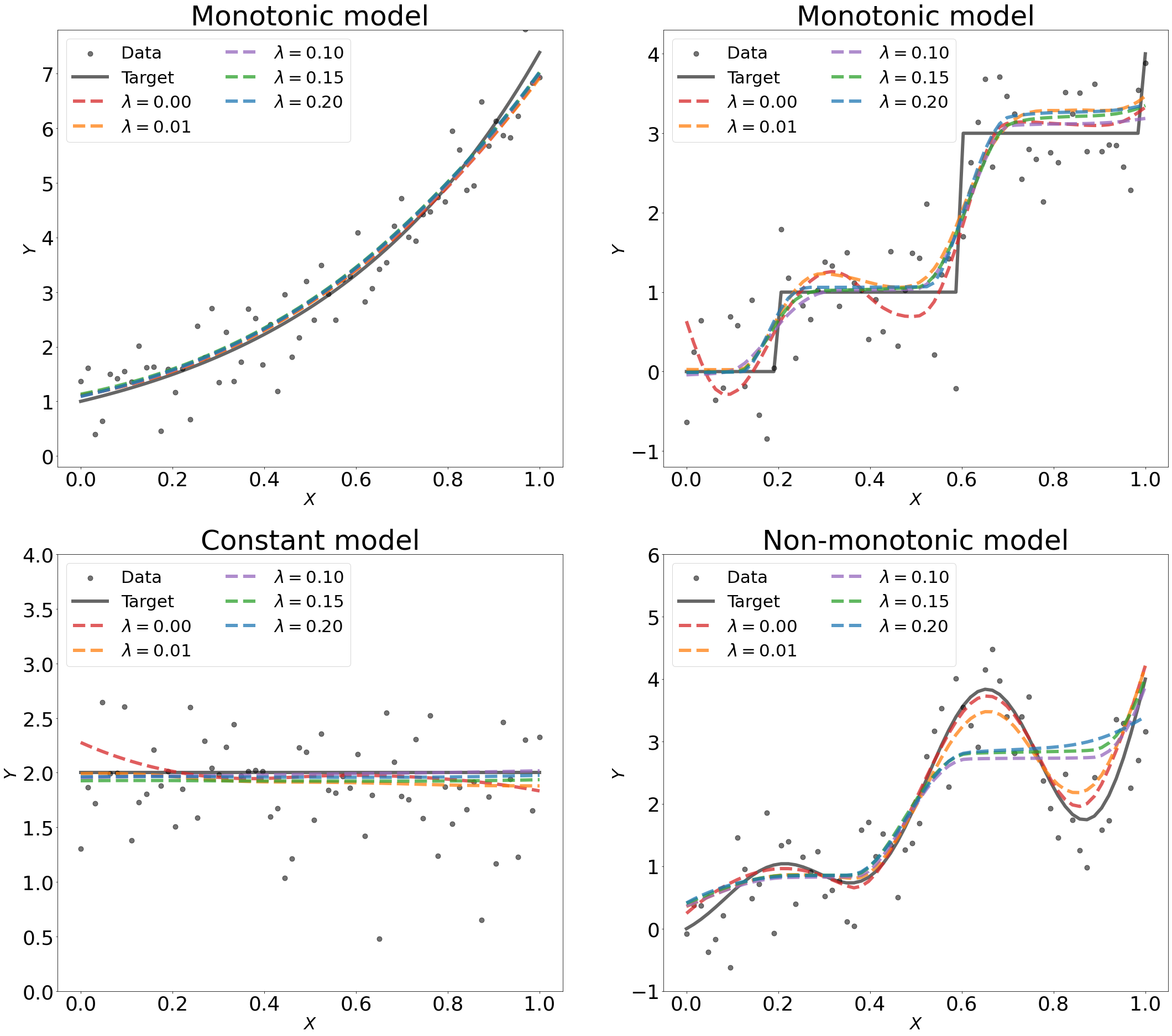
Figure 1: Examples of PDIR estimates. In all figures, the data points are depicted as grey dots, the underlying regression functions are plotted as solid black curves, and PDIR estimates with different level of penalty parameter $\lambda$ are plotted as colored curves. In the top two figures, data are generated from models with monotonic regression functions. In the bottom left figure, the target function is a constant. In the bottom right figure, the model is misspecified, in which the underlying regression function is not monotonic. Small values of $\lambda$ can lead to non-monotonic estimated functions.

An illustration of PDIR is presented in Figure 1. In all subfigures, the data are depicted as grey dots, the underlying regression functions are plotted as solid black curves and PDIR estimates with different levels of penalty parameter $\lambda$ are plotted as colored curves. In the top two figures, data are generated from models with monotonic regression functions. In the bottom left figure, the target function is a constant. In the bottom right figure, the model is misspecified, in which the underlying regression function is not monotonic. Small values of $\lambda$ can lead to non-monotonic and reasonable estimates, suggesting that PDIR is robust against model misspecification. We have conducted more numerical experiments to evaluate the performance of PDIR, which indicate that PDIR tends to perform better than the existing isotonic regression methods considered in the comparison. The results are given in the Supplementary Material.

5.1 Non-asymptotic error bounds for PDIR

This section presents the main findings regarding the bounds for the excess risk of the PDIR estimator, as defined in (12). Let $R^{\lambda}$ be defined in (6). For notational simplicity, we write

$$\mathcal{R}(f)=\mathcal{R}^{0}(f)=\mathbb{E}|Y-f(X)|^{2}.$$

Recall that the target $f_{0}$ is defined as the measurable function that minimizes the risk $\mathcal{R}(f)$, i.e., $f_{0}\in\arg\min_{f}\mathcal{R}(f).$ In isotonic regression, we assume that $f_{0}\in\mathcal{F}_{0}.$ In addition, for any function $f$, under the regression model (4), we have

$$\mathcal{R}(f)-\mathcal{R}(f_{0})=\mathbb{E}|f(X)-f_{0}(X)|^{2}.$$

The excess risk bounds are established under certain conditions, which we state below.

Assumption 4.

(i) The target regression function $f_{0}:\mathcal{X}\to\mathbb{R}$ defined in (4) is coordinate-wisely nondecreasing on $\mathcal{X}$, i.e., $f_{0}(x)\leq f_{0}(y)$ if $x\preceq y$ for $x,y\in\mathcal{X}\subseteq\mathbb{R}^{d}$. (ii) The errors $\epsilon_{i},i=1,\ldots,n,$ are independent and identically distributed noise variables with $\mathbb{E}(\epsilon_{i})=0$ and ${\rm Var}(\epsilon_{i})\leq\sigma^{2}$, and $\epsilon_{i}$’s are independent of $\{X_{i}\}_{i=1}^{n}$.

Assumption 4 includes basic model assumptions on the errors and the monotonic target function $f_{0}$. In addition, we assume that the target function $f_{0}$ belongs to the class $C^{s}$.

Next, the following lemma provides a preliminary upper bound on the excess risk of $\hat{f}^{\lambda}_{n}$ defined in (12).

Lemma 4 (Excess risk decomposition).

The excess risk of the empirical risk minimizer $\hat{f}^{\lambda}_{n}$ defined in (12) satisfies

$$\mathbb{E}|\hat{f}^{\lambda}_{n}(X)-f_{0}(X)|^{2}= \mathbb{E}\Big{\{}\mathcal{R}(\hat{f}_{n}^{\lambda})-\mathcal{R}(f_{0})\Big{\}}\leq\mathbb{E}\Big{\{}\mathcal{R}^{\lambda}(\hat{f}_{n}^{\lambda})-\mathcal{R}^{\lambda}(f_{0})\Big{\}}$$

$$\leq \mathbb{E}\Big{\{}\mathcal{R}^{\lambda}(\hat{f}^{\lambda}_{n})-2\mathcal{R}^{\lambda}_{n}(\hat{f}^{\lambda}_{n})+\mathcal{R}^{\lambda}(f_{0})\Big{\}}+2\inf_{f\in\mathcal{F}_{n}}\Big{[}\mathcal{R}^{\lambda}(f)-\mathcal{R}^{\lambda}(f_{0})\Big{]}.$$

The upper bound for the excess risk can be decomposed into two components: the stochastic error, given by the expected value of $\mathcal{R}^{\lambda}(\hat{f}^{\lambda}_{n})-2\mathcal{R}^{\lambda}_{n}(\hat{f}^{\lambda}_{n})+\mathcal{R}^{\lambda}(f_{0})$, and the approximation error, defined as $\inf_{f\in\mathcal{F}_{n}}[\mathcal{R}^{\lambda}(f)-\mathcal{R}^{\lambda}(f_{0})]$. To establish a bound for the stochastic error, it is necessary to consider the complexities of both RePU networks and their derivatives, which have been investigated in our Theorem 1 and Lemma 1. To establish a bound for the approximation error $\inf_{f\in\mathcal{F}_{n}}{\mathcal{R}^{\lambda}(f)-\mathcal{R}^{\lambda}(f_{0})}$, we rely on the simultaneous approximation results derived in Theorem 3.

Remark 4.

The error decomposition presented in Lemma 4 differs from the canonical decomposition for score estimation, as given in section 4.1, particularly with respect to the stochastic error component. However, utilizing the decomposition in Lemma 4 enables us to derive a superior stochastic error bound by leveraging the properties of the PDIR loss function. A similar decomposition for least squares loss without penalization has also been used in Jiao et al. (2021a).

Lemma 5.

Suppose that Assumptions 3, 4 hold and the target function $f_{0}$ defined in (4) belongs to $C^{s}$ for some $s\in\mathbb{N}^{+}$. For any positive odd number $\mathcal{D}$, let $\mathcal{F}_{n}:=\mathcal{F}_{\mathcal{D},\mathcal{W},\mathcal{U},\mathcal{S},\mathcal{B},\mathcal{B}^{\prime}}$ be the class of RePU activated neural networks $f:\mathcal{X}\to\mathbb{R}^{d}$ with depth $\mathcal{D}$, width $\mathcal{W}=18pd[(\mathcal{D}+1)/2]^{d-1}$, number of neurons $\mathcal{U}=18pd[(\mathcal{D}+1)/2]^{d}$ and size $\mathcal{S}=67pd[(\mathcal{D}+1)/2]^{d}$. Suppose that $\mathcal{B}\geq\|f_{0}\|_{C^{0}}$ and $\mathcal{B}^{\prime}\geq\|f_{0}\|_{C^{1}}$. Then for $n\geq\max\{{\rm Pdim}(\mathcal{F}_{n}),{\rm Pdim}(\mathcal{F}^{\prime}_{n})\}$, the excess risk of PDIR $\hat{f}^{\lambda}_{n}$ defined in (12) satisfies

$$\mathbb{E}|\hat{f}^{\lambda}_{n}(X)-f_{0}(X)|^{2} \leq\mathcal{E}_{sto}+\mathcal{E}_{app},$$ (13)

$$\mathbb{E}\big{[}\frac{1}{d}\sum_{j=1}^{d}\lambda_{j}\rho(\frac{\partial}{\partial x_{j}}\hat{f}^{\lambda}_{n}(X))\big{]} \leq\mathcal{E}_{sto}+\mathcal{E}_{app},$$ (14)

with

$$\mathcal{E}_{sto} =C_{1}d\big{\{}p^{3}\mathcal{B}^{3}+d(\kappa\bar{\lambda}\mathcal{B}^{\prime})^{2}\big{\}}(\log n)n^{-1}\mathcal{U}^{(d+2)/d},$$

$$\mathcal{E}_{app} =C_{2}(1+\kappa\bar{\lambda})\|f_{0}\|^{2}_{C^{s}}\mathcal{U}^{-(s-1)/d},$$

where the expectation $\mathbb{E}$ is taken with respect to $X$ and $\hat{f}^{\lambda}_{n}$, $\bar{\lambda}=\sum_{j=1}^{d}\lambda_{j}/d$ is the mean of the tuning parameters, $C_{1}>0$ is a universal constant and $C_{2}>0$ is a positive constant depending only on $d,s$ and the diameter of the support $\mathcal{X}$.

Lemma 5 establishes two error bounds for the PDIR estimator $\hat{f}^{\lambda}_{n}$: (13) for the mean squared error between $\hat{f}^{\lambda}_{n}$ and the target $f_{0}$, and (14) for controlling the non-monotonicity of $\hat{f}^{\lambda}_{n}$ via its partial derivatives $\frac{\partial}{\partial x_{j}}\hat{f}_{n},j=1,\ldots,d,$ with respect to a measure defined in terms of $\rho$. It is noteworthy that both bounds are equivalent in terms of their value, and encompass both stochastic and approximation errors. Specifically, the stochastic error is of order $\mathcal{O}(\mathcal{U}^{(d+2)/d}/n)$, which represents an improvement over the canonical error bound of $\mathcal{O}([\mathcal{U}^{(d+2)/d}/n]^{1/2})$, up to logarithmic factors in $n$. This advancement arises from the application of the decomposition in Lemma 4 and the utilization of the properties of PDIR loss function, rather than relying on traditional decomposition techniques.

Remark 5.

In (14), the estimator $\hat{f}^{\lambda}_{n}$ is encouraged to exhibit monotonicity, as the expected monotonicity penalty on the estimator $\mathbb{E}[\frac{1}{d}\sum{j=1}^{d}\lambda_{j}\rho(\frac{\partial}{\partial x_{j}}\hat{f}^{\lambda}_{n}(X))]$ is bounded. Clearly, when $\mathbb{E}[\rho(\frac{\partial}{\partial x_{j}}\hat{f}^{\lambda}_{n}(X))]=0$, the estimator $\hat{f}^{\lambda}_{n}$ is almost surely monotonic in its $j$th argument with respect to the probability measure of $X$. Based on (14), guarantees of the estimator’s monotonicity with respect to a single argument can be obtained. Specifically, for those $j$ where $\lambda_{j}\not=0$, we have $\mathbb{E}[\rho(\frac{\partial}{\partial x_{j}}\hat{f}^{\lambda}_{n}(X))]\leq d(\mathcal{E}_{sto}+\mathcal{E}_{app})/\lambda_{j}$, which provides a guarantee of the estimator’s monotonicity with respect to its $j$th argument. Notably, larger values of $\lambda_{j}$ lead to smaller bounds, which is consistent with the intuition that larger values of $\lambda_{j}$ better promote monotonicity of $\hat{f}^{\lambda}_{n}$ with respect to its $j$th argument.

Theorem 7 (Non-asymptotic excess risk bounds).

Under the conditions of Lemma 5 to achieve the smallest error bound in (13), we can set $\mathcal{U}=18pd\lfloor n^{d/(d+s+1)}\rfloor$ and $\lambda_{j}=\log n$ for $j=1,\ldots,d$. Then we have

$$\mathbb{E}|\hat{f}^{\lambda}_{n}(X)-f_{0}(X)|^{2} \leq C(\log n)^{2}n^{-\frac{s-1}{d+s+1}},$$

and

$$\mathbb{E}[\rho(\frac{\partial}{\partial x_{j}}\hat{f}^{\lambda}_{n}(X))]\leq C(\log n)n^{-\frac{s-1}{d+s+1}},$$

for $j=1,\ldots,d$, where $C>0$ is a constant only depending on $\mathcal{B},\mathcal{B}^{\prime},s,d,\mathcal{X},\|f_{0}\|_{C^{s}}$ and $\kappa$.

The term $-(s-1)$ in the exponent of the convergence rate is due to the approximation of the first-order partial derivative of the target function. Of course, the smoothness of the target function $f_{0}$ is unknown in practice and how to determine the smoothness of an unknown function is an important but nontrivial problem. Note the convergence rate $(\log n)^{2}n^{-(s-1)/(d+s+1)}$ The convergence rate suffers from the curse of dimensionality, since it can be extremely slow if $d$ is large.

Remark 6.

In Theorem 7, we choose $\lambda_{j}=\log n,\ j=1,\ldots,d,$ to attain the optimal rate of the expected mean squared error of $\hat{f}^{\lambda}_{n}$ up to a logarithmic factor. Additionally, we guarantee that the estimator $\hat{f}^{\lambda}_{n}$ to be monotonic at a rate of $n^{-(s-1)/(d+s+1)}$ up to a logarithmic factor as measured by $\mathbb{E}[\rho(\frac{\partial}{\partial x_{j}}\hat{f}^{\lambda}_{n}(X))]$. The choice of $\lambda_{j}$ is not unique for ensuring the consistency of $\hat{f}^{\lambda}_{n}$. In fact, any choice of $\bar{\lambda}=o((\log n)^{-1}n^{(s-1)/(d+s+1)})$ will result in a consistent $\hat{f}^{\lambda}_{n}$. However, larger values of $\bar{\lambda}$ lead to a slower convergence rate of the expected mean squared error, but provide better guarantee for the monotonicity of $\hat{f}^{\lambda}_{n}$.

High-dimensional data can have low-dimensional latent structures in applications. Below we show that PDIR can mitigate the curse of dimensionality if the data distribution is supported on an approximate low-dimensional manifold.

Lemma 6.

Suppose that Assumptions 1, 3, 4 hold and the target function $f_{0}$ defined in (4) belongs to $C^{s}$ for some $s\in\mathbb{N}^{+}$. For any $\delta\in(0,1)$, let $d_{\delta}=O(d_{\mathcal{M}}\log(d/\delta)/\delta^{2})$ be an integer with $d_{\delta}\leq d$. For any positive even number $\mathcal{D}$, let $\mathcal{F}_{n}:=\mathcal{F}_{\mathcal{D},\mathcal{W},\mathcal{U},\mathcal{S},\mathcal{B},\mathcal{B}^{\prime}}$ be the class of RePU activated neural networks $f:\mathcal{X}\to\mathbb{R}^{d}$ with depth $\mathcal{D}$, width $\mathcal{W}=18pd[\mathcal{D}/2]^{d_{\delta}-1}$, number of neurons $\mathcal{U}=18pd[\mathcal{D}/2]^{d_{\delta}}$ and size $\mathcal{S}=67pd[\mathcal{D}/2]^{d_{\delta}}$ Suppose that $\mathcal{B}\geq\|f_{0}\|_{C^{0}}$ and $\mathcal{B}^{\prime}\geq\|f_{0}\|_{C^{1}}$. Then for $n\geq\max\{{\rm Pdim}(\mathcal{F}_{n}),{\rm Pdim}(\mathcal{F}^{\prime}_{n})\}$, the excess risk of the PDIR estimator $\hat{f}^{\lambda}_{n}$ defined in (12) satisfies

$$\mathbb{E}|\hat{f}^{\lambda}_{n}(X)-f_{0}(X)|^{2} \leq\mathcal{E}_{sto}+\tilde{\mathcal{E}}_{app},$$ (15)

$$\mathbb{E}\big{[}\frac{1}{d}\sum_{j=1}^{d}\lambda_{j}\rho(\frac{\partial}{\partial x_{j}}\hat{f}^{\lambda}_{n}(X))\big{]} \leq\mathcal{E}_{sto}+\tilde{\mathcal{E}}_{app},$$ (16)

with

$$\mathcal{E}_{sto} =C_{1}d\big{\{}p^{3}\mathcal{B}^{3}+d(\kappa\bar{\lambda}\mathcal{B}^{\prime})^{2}\big{\}}(\log n)n^{-1}\mathcal{U}^{(d+2)/d},$$

$$\tilde{\mathcal{E}}_{app} =C_{2}(1+\kappa\bar{\lambda})\|f_{0}\|^{2}_{C^{s}}\mathcal{U}^{-(s-1)/d_{\delta}},$$

for $\rho\leq C_{\rho}\mathcal{U}^{-(s-|\alpha|_{1})/d_{\delta}}(1+\delta)^{-1},$ where $C_{\rho},C_{1}>0$ are universal constants and $C_{2}>0$ is a constant depending only on $d_{\delta},s$ and the diameter of the support $\mathcal{M}_{\rho}$.

Based on Lemma 6, we obtain the following result.

Theorem 8 (Improved non-asymptotic excess risk bounds).

Under the conditions of Lemma 6, to achieve the smallest error bound in (15), we can set $\mathcal{U}=18pd\lfloor n^{d_{\delta}/(d_{\delta}+s+1)}\rfloor$ and $\lambda_{=}\log n$ for $j=1,\ldots,d$. Then we have

$$\mathbb{E}|\hat{f}^{\lambda}_{n}(X)-f_{0}(X)|^{2} \leq C(\log n)^{2}n^{-\frac{s-1}{d_{\delta}+s+1}},$$

and for $j=1,\ldots,d$,

$$\mathbb{E}[\rho(\frac{\partial}{\partial x_{j}}\hat{f}^{\lambda}_{n}(X))]\leq C(\log n)n^{-\frac{s-1}{d_{\delta}+s+1}},$$

where $C>0$ is a constant only depending on $\mathcal{B},\mathcal{B}^{\prime},s,d,d_{\delta},\mathcal{M}_{\rho},\|f_{0}\|_{C^{s}}$ and $\kappa$.

In Theorem 8, the effective dimension is $d_{\delta}$ instead of large $d$. Therefore, the rate of convergence is an improvement over the result in Theorem 7 when the intrinsic dimension $d_{\delta}$ is smaller than the ambient dimension $d$.

5.2 PDIR under model misspecification

In this subsection, we investigate PDIR under model misspecification when Assumption 4 (i) is not satisfied, meaning that the underlying regression function $f_{0}$ may not be monotonic.

Let $S:={(X_{i},Y_{i})}_{i=1}^{n}$ be a random sample from model (4). Recall that the penalized risk of the deep isotonic regression is given by

$$\mathcal{R}^{\lambda}(f)=\mathbb{E}|Y-f(X)|^{2}+\frac{1}{d}\sum_{j=1}^{d}\lambda_{j}\mathbb{E}{\rho(\dot{f}_{j}(X))},$$

If $f_{0}$ is not monotonic, then the penalty $\sum_{j=1}^{d}\lambda_{j}\mathbb{E}[\rho(\dot{f}_{j}(X))/d]$ is non-zero, and consequently, $f_{0}$ is not a minimizer of the risk $\mathcal{R}^{\lambda}$ when $\lambda_{j}\not=0,\forall j$. Intuitively, the deep isotonic regression estimator will exhibit a bias towards the target $f_{0}$ due to the additional penalty terms in the risk. However, it is reasonable to expect that the estimator $\hat{f}^{\lambda}_{n}$ will have a smaller bias if the $\lambda_{j},j=1,\ldots,d$ values are small. In the following lemma, we establish a non-asymptotic upper bound for our proposed deep isotonic regression estimator while adapting to model misspecification.

Lemma 7.

Suppose that Assumptions 3 and 4 (ii) hold and the target function $f_{0}$ defined in (4) belongs to $C^{s}$ for some $s\in\mathbb{N}^{+}$. For any positive odd number $\mathcal{D}$, let $\mathcal{F}_{n}:=\mathcal{F}_{\mathcal{D},\mathcal{W},\mathcal{U},\mathcal{S},\mathcal{B},\mathcal{B}^{\prime}}$ be the class of RePU activated neural networks $f:\mathcal{X}\to\mathbb{R}^{d}$ with depth $\mathcal{D}$, width $\mathcal{W}=18pd[(\mathcal{D}+1)/2]^{d-1}$, number of neurons $\mathcal{U}=18pd[(\mathcal{D}+1)/2]^{d}$ and size $\mathcal{S}=67pd[(\mathcal{D}+1)/2]^{d}$. Suppose that $\mathcal{B}\geq\|f_{0}\|_{C^{0}}$ and $\mathcal{B}^{\prime}\geq\|f_{0}\|_{C^{1}}$. Then for $n\geq\max\{{\rm Pdim}(\mathcal{F}_{n}),{\rm Pdim}(\mathcal{F}^{\prime}_{n})\}$, the excess risk of the PDIR estimator $\hat{f}^{\lambda}_{n}$ defined in (12) satisfies

$$\mathbb{E}|\hat{f}^{\lambda}_{n}(X)-f_{0}(X)|^{2}\leq \mathcal{E}_{sto}+\mathcal{E}_{app}+\mathcal{E}_{mis},$$ (17)

$$\mathbb{E}\big{[}\frac{1}{d}\sum_{j=1}^{d}\lambda_{j}\rho(\frac{\partial}{\partial x_{j}}\hat{f}^{\lambda}_{n}(X))\big{]} \leq\mathcal{E}_{sto}+\mathcal{E}_{app}+\mathcal{E}_{mis},$$ (18)

with

$$\mathcal{E}_{sto} =C_{1}p^{2}d^{3}(\mathcal{B}^{2}+\kappa\bar{\lambda}\mathcal{B}^{\prime})(\log n)^{1/2}n^{-1/2}\mathcal{U}^{(d+2)/2d},$$

$$\mathcal{E}_{app} =C_{2}(1+\kappa\bar{\lambda})\|f_{0}\|^{2}_{C^{s}}\mathcal{U}^{-(s-1)/d},$$

$$\mathcal{E}_{mis} =\frac{1}{d}\sum_{j=1}^{d}\lambda_{j}\mathbb{E}[\rho(\frac{\partial}{\partial x_{j}}f_{0}(X))],$$

where the expectation $\mathbb{E}$ is taken with respect to $X$ and $\hat{f}^{\lambda}_{n}$, $\bar{\lambda}=\sum_{j=1}^{d}\lambda_{j}/d$ is the mean of the tuning parameters, $C_{1}>0$ is a universal constant and $C_{2}>0$ is a positive constant depending only on $d,s$ and the diameter of the support $\mathcal{X}$.

Lemma 7 is a generalized version of Lemma 5 for PDIR, as it holds regardless of whether the target function is isotonic or not. In Lemma 7, the expected mean squared error of the PDIR estimator $\hat{f}^{\lambda}_{n}$ can be bounded by three errors: stochastic error $\mathcal{E}_{sto}$, approximation error $\mathcal{E}_{app}$, and misspecification error $\mathcal{E}_{mis}$, without the monotonicity assumption. Compared with Lemma 5 with the monotonicity assumption, the approximation error is identical, the stochastic error is worse in terms of order, and the misspecification error appears as an extra term in the inequality. With an appropriate setup of the number of neurons $\mathcal{U}$ of the neural network with respect to the sample size $n$, the stochastic error and approximation error can converge to zero, albeit at a slower rate than that in Theorem 7. However, the misspecification error remains constant for fixed tuning parameters $\lambda_{j}$. Thus, we can let the tuning parameters $\lambda_{j}$ converge to zero to achieve consistency.

Remark 7.

It is worth noting that if the target function is isotonic, then the misspecification error vanishes, reducing the scenario to that of isotonic regression. However, the convergence rate based on Lemma 7 is slower than that in Lemma 5. The reason is that Lemma 7 is general and holds without prior knowledge of the monotonicity of the target function. If knowledge is available about the non-isotonicity of the $j$th argument of the target function $f_{0}$, setting the corresponding $\lambda_{j}=0$ decreases the misspecification error and helps improve the upper bound.

Theorem 9 (Non-asymptotic excess risk bounds).

Under the conditions of Lemma 7, to achieve the smallest error bound in (17), we can set $\mathcal{U}=18pd\lfloor n^{d/(d+2s)}\rfloor$ and $\lambda_{j}=(\log n)^{\alpha}n^{-(s-1)/(d+2s)}$ for $j=1,\ldots,d$ and some $\alpha>1$ . Then we have

$$\mathbb{E}|\hat{f}^{\lambda}_{n}(X)-f_{0}(X)|^{2} \leq C(\log n)n^{-\frac{s-1}{d+2s}},$$

where $C>0$ is a constant only depending on $\mathcal{B},\mathcal{B}^{\prime},s,d,\mathcal{X},\|f_{0}\|_{C^{s}}$ and $\kappa$.

Remark 8.

There is no unique choice of $\lambda_{j}$ that ensures the consistency of PDIR, as proven in Theorem 9. Consistency is, in fact, guaranteed even under a misspecified model when the $\lambda_{j}$ for $j=1,\ldots,d$ tend to zero as $n\to\infty$. Additionally, selecting a smaller value of $\bar{\lambda}$ provides a better upper bound for (17), and an optimal rate up to logarithms of $n$ can be achieved with a sufficiently small $\bar{\lambda}=O(n^{-(s-1)/(d+2s)})$. An example demonstrating the effects of tuning parameters is visualized in the last subfigure of Figure 1.

6 Related works

In this section, we give a brief review of the papers in the existing literature that are most related to the present work.

6.1 ReLU and RePU networks

Deep learning has achieved impressive successes in a wide range of applications. A fundamental reason for these successes is the ability of deep neural networks in approximating high-dimensional functions and extracting effective data representations. There has been much effort devoted to studying the approximation properties of deep neural networks in recent years. Many interesting results have been obtained concerning the approximation power of deep neural networks for multivariate functions. Examples include Yarotsky (2017, 2018); Lu et al. (2017); Raghu et al. (2017); Shen, Yang and Zhang (2019); Shen, Yang and Zhang (2020); Chen, Jiang and Zhao (2019); Schmidt-Hieber (2020); Jiao et al. (2021b). These works focused on the power of ReLU activated neural networks for approximating various types of smooth functions.

For the approximation of the square function by ReLU networks, Yarotsky (2017) first used “sawtooth” functions, which achieves an error rate of $\mathcal{O}(2^{-L})$ with width 6 and depth $\mathcal{O}(L)$ for any positive integer $L\in\mathbb{N}^{+}$. General construction of ReLU networks for approximating a square function can achieve an error $N^{-L}$ with width $3N$ and depth $L$ for any positive integers $N,L\in\mathbb{N}^{+}$ (Lu et al., 2021a). Based on this basic fact, the ReLU networks approximating multiplication and polynomials can be constructed correspondingly. However, the network complexity in terms of network size (depth and width) for a ReLU network to achieve precise approximation can be large compared to that of a RePU network since RePU network can exactly compute polynomials with fewer layers and neurons.

The approximation results of RePU network are generally obtained by converting splines or polynomials into RePU networks and make use the approximation results of splines and polynomials. The universality of sigmoidal deep neural networks have been studied in the pioneering works (Mhaskar, 1993; Chui, Li and Mhaskar, 1994). In addition, the approximation properties of shallow Rectified Power Unit (RePU) activated network were studied in Klusowski and Barron (2018); Siegel and Xu (2022). The approximation rates of deep RePU neural networks on target functions in different spaces have also been explored, including Besov spaces (Ali and Nouy, 2021), Sobolev spaces (Li, Tang and Yu, 2019a, b; Duan et al., 2021; Abdeljawad and Grohs, 2022) , and Hölder space (Belomestny et al., 2022). Most of the existing results on the expressiveness of neural networks measure the quality of approximation with respect to $L_{p}$ where $p\geq 1$ norm. However, fewer papers have studied the approximation of derivatives of smooth functions (Duan et al., 2021; Gühring and Raslan, 2021; Belomestny et al., 2022).

6.2 Related works on score estimation

Learning a probability distribution from data is a fundamental task in statistics and machine learning for efficient generation of new samples from the learned distribution. Likelihood-based models approach this problem by directly learning the probability density function, but they have several limitations, such as an intractable normalizing constant and approximate maximum likelihood training.

One alternative approach to circumvent these limitations is to model the score function (Liu, Lee and Jordan, 2016), which is the gradient of the logarithm of the probability density function. Score-based models can be learned using a variety of methods, including parametric score matching methods (Hyvärinen and Dayan, 2005; Sasaki, Hyvärinen and Sugiyama, 2014), autoencoders as its denoising variants (Vincent, 2011), sliced score matching (Song et al., 2020), nonparametric score matching (Sriperumbudur et al., 2017; Sutherland et al., 2018), and kernel estimators based on Stein’s methods (Li and Turner, 2017; Shi, Sun and Zhu, 2018). These score estimators have been applied in many research problems, such as gradient flow and optimal transport methods (Gao et al., 2019, 2022), gradient-free adaptive MCMC (Strathmann et al., 2015), learning implicit models (Warde-Farley and Bengio, 2016), inverse problems (Jalal et al., 2021). Score-based generative learning models, especially those using deep neural networks, have achieved state-of-the-art performance in many downstream tasks and applications, including image generation (Song and Ermon, 2019, 2020; Song et al., 2021; Ho, Jain and Abbeel, 2020; Dhariwal and Nichol, 2021; Ho et al., 2022), music generation (Mittal et al., 2021), and audio synthesis (Chen et al., 2020; Kong et al., 2020; Popov et al., 2021).

However, there is a lack of theoretical understanding of nonparametric score estimation using deep neural networks. The existing studies mainly considered kernel based methods. Zhou, Shi and Zhu (2020) studied regularized nonparametric score estimators using vector-valued reproducing kernel Hilbert space, which connects the kernel exponential family estimator (Sriperumbudur et al., 2017) with the score estimator based on Stein’s method (Li and Turner, 2017; Shi, Sun and Zhu, 2018). Consistency and convergence rates of these kernel-based score estimator are also established under the correctly-specified model assumption in Zhou, Shi and Zhu (2020). For denoising autoencoders, Block, Mroueh and Rakhlin (2020) obtained generalization bounds for general nonparametric estimators also under the correctly-specified model assumption.

For sore-based learning using deep neural networks, the main difficulty for establishing the theoretical foundation is the lack of knowledge of differentiable neural networks since the derivatives of neural networks are involved in the estimation of score function. Previously, the non-differentiable Rectified Linear Unit (ReLU) activated deep neural network has received much attention due to its attractive properties in computation and optimization, and has been extensively studied in terms of its complexity (Bartlett, Maiorov and Meir, 1998; Anthony and Bartlett, 1999; Bartlett et al., 2019) and approximation power (Yarotsky, 2017; Petersen and Voigtlaender, 2018; Shen, Yang and Zhang, 2020; Lu et al., 2021b; Jiao et al., 2021a), based on which statistical learning theories for deep non-parametric estimations were established (Bauer and Kohler, 2019; Schmidt-Hieber, 2020; Jiao et al., 2021a). For deep neural networks with differentiable activation functions, such as ReQU and RepU, the simultaneous approximation power on a smooth function and its derivatives were studied recently (Ali and Nouy, 2021; Belomestny et al., 2022; Siegel and Xu, 2022; Hon and Yang, 2022), but the statistical properties of differentiable networks are still largely unknown. To the best of our knowledge, the statistical learning theory has only been investigated for ReQU networks in Shen et al. (2022), where they have developed network representation of the derivatives of ReQU networks and studied their complexity.

6.3 Related works on isotonic regression

There is a rich and extensive literature on univariate isotonic regression, which is too vast to be adequately summarized here. So we refer to the books Barlow et al. (1972) and Robertson, Wright and Dykstra (1988) for a systematic treatment of this topic and review of earlier works. For more recent developments on the error analysis of nonparametric isotonic regression, we refer to Durot (2002); Zhang (2002); Durot (2007, 2008); Groeneboom and Jongbloed (2014); Chatterjee, Guntuboyina and Sen (2015), and Yang and Barber (2019), among others.

The least squares isotonic regression estimators under fixed design were extensively studied. With a fixed design at fixed points $x_{1},\ldots,x_{n}$, the $L_{p}$ risk of the least squares estimator is defined by $\mathcal{R}_{n,p}(\hat{f}_{0})=\mathbb{E}(n^{-1}\sum_{i=1}^{n}|\hat{f}_{0}(x_{i})-f_{0}(x_{i})|^{p})^{1/p},$ where the least squares estimator $\hat{f}_{0}$ is defined by

$$\hat{f}_{0}=\arg\min_{f\in\mathcal{F}_{0}}\frac{1}{n}\sum_{i=1}^{n}(Y_{i}-f(x_{i}))^{2}.$$ (19)

The problem can be restated in terms of isotonic vector estimation on directed acyclic graphs. Specifically, the design points $\{x_{1},\ldots,x_{n}\}$ induce a directed acyclic graph $G_{x}(V(G_{x}),E(G_{x}))$ with vertices $V(G_{x})=\{1,\ldots,n\}$ and edges $E(G_{x})=\{(i,j):x_{i}\preceq x_{j}\}$. The class of isotonic vectors on $G_{x}$ is defined by

$$\mathcal{M}(G):=\{\theta\in\mathbb{R}^{V(G_{x})}:\theta_{x}\leq\theta_{y}{\rm\ for}x\preceq y\}.$$

Then the least squares estimation in (19) becomes that of searching for a target vector $\theta_{0}=\{(\theta_{0})_{i}\}_{i=1}^{n}:=\{f_{0}(x_{i})\}_{i=1}^{n}\in\mathcal{M}(G_{x})$. The least squares estimator $\hat{\theta}_{0}=\{(\hat{\theta}_{0})_{i}\}_{i=1}^{:}=\{\hat{f}_{0}(x_{i})\}_{i=1}^{n}$ is actually the projection of $\{Y_{i}\}_{i=1}^{n}$ onto the polyhedral convex cone $\mathcal{M}(G_{x})$ (Han et al., 2019). For univariate isotonic least squares regression with a bounded total variation target function $f_{0}$, Zhang (2002) obtained sharp upper bounds for $\mathcal{R}_{n,p}$ risk of the least squares estimator $\hat{\theta}_{0}$ for $1\leq p<3$.

Shape-constrained estimators were also considered in different settings where automatic rate-adaptation phenomenon happens (Chatterjee, Guntuboyina and Sen, 2015; Gao, Han and Zhang, 2017; Bellec, 2018). We also refer to Kim, Guntuboyina and Samworth (2018); Chatterjee and Lafferty (2019) for other examples of adaptation in univariate shape-constrained problems. Error analysis for the least squares estimator in multivariate isotonic regression is more difficult. For two-dimensional isotonic regression, where $X\in\mathbb{R}^{d}$ with $d=2$ and Gaussian noise, Chatterjee, Guntuboyina and Sen (2018) considered the fixed lattice design case and obtained sharp error bounds. Han et al. (2019) extended the results of Chatterjee, Guntuboyina and Sen (2018) to the case with $d\geq 3$, both from a worst-case perspective and an adaptation point of view. They also proved parallel results for random designs assuming the density of the covariate $X$ is bounded away from zero and infinity on the support.

Deng and Zhang (2020) considered a class of block estimators for multivariate isotonic regression in $\mathbb{R}^{d}$ involving rectangular upper and lower sets under, which is defined as any estimator in-between the following max-min and min-max estimator. Under a $q$-th moment condition on the noise, they developed $L_{q}$ risk bounds for such estimators for isotonic regression on graphs.

Furthermore, the block estimator possesses an oracle property in variable selection: when $f_{0}$ depends on only an unknown set of $s$ variables, the $L_{2}$ risk of the block estimator automatically achieves the minimax rate up to a logarithmic factor based on the knowledge of the set of the $s$ variables.

Our proposed method and theoretical results are different from those in the aforementioned papers in several aspects. First, the resulting estimates from our method are smooth instead of piecewise constant as those based on the existing methods. Second, our method can mitigate the curse of dimensionality under an approximate low-dimensional manifold support assumption, which is weaker than the exact low-dimensional space assumption in the existing work. Finally, our method possesses a robustness property against model specification in the sense that it still yields consistent estimators if the monotonicity assumption is not strictly satisfied. However, the properties of the existing isotonic regression methods under model misspecification are not clear.

7 Conclusions

In this work, motivated by the problems of score estimation and isotonic regression, we have studied the properties of RePU-activated neural networks, including a novel generalization result for the derivatives of RePU networks and improved approximation error bounds for RePU networks with approximate low-dimensional structures. We have established non-asymptotic excess risk bounds for DSME, a deep score matching estimator; and PDIR, our proposed penalized deep isotonic regression method.

Our findings highlight the potential of RePU-activated neural networks in addressing challenging problems in machine learning and statistics. The ability to accurately represent the partial derivatives of RePU networks with RePUs mixed-activated networks is a valuable tool in many applications that require the use of neural network derivatives. Moreover, the improved approximation error bounds for RePU networks with low-dimensional structures demonstrate their potential to mitigate the curse of dimensionality in high-dimensional settings.

Future work can investigate further the properties of RePU networks, such as their stability, robustness, and interpretability. It would also be interesting to explore the use of RePU-activated neural networks in other applications, such as nonparametric variable selection and more general shape-constrained estimation problems. Additionally, our work can be extended to other smooth activation functions beyond RePUs, such as Gaussian error linear unit and scaled exponential linear unit, and study their derivatives and approximation properties.

Supplementary material

The supplementary material contains the proofs and supporting lemmas for the theoretical results, as well as results from simulation studies to evaluate the performance of PDIR.

This supplement contains results from simulation studies to evaluate the performance of PDIR and proofs and supporting lemmas for the theoretical results stated in the paper.

Appendix A Numerical studies

In this appendix, we conduct simulation studies to evaluate the performance of PDIR and compare it with the existing isotonic regression methods. The methods included in the simulation include

• The isotonic least squares estimator, denoted by Isotonic LSE, is defined as the minimizer of the mean square error on the training data subject to the monotone constraint. As the squared loss only involves the values at $n$ design points, then the isotonic LSE (with no more than $\binom{n}{2}$ linear constraints) can be computed with quadratic programming or using convex optimization algorithms (Dykstra, 1983; Kyng, Rao and Sachdeva, 2015; Stout, 2015). Algorithmically, this turns out to be mappable to a network flow problem (Picard, 1976; Spouge, Wan and Wilbur, 2003). In our implementation, we compute Isotonic LSE via the Python package multiisotonic.

• The block estimator (Deng and Zhang, 2020), denoted by Block estimator, is defined as any estimator between the block min-max and max-min estimators (Fokianos, Leucht and Neumann, 2020). In the simulation, we take the Block estimator as the mean of max-min and min-max estimators as suggested in (Deng and Zhang, 2020). The Isotonic LSE is shown to has an explicit mini-max representation on the design points for isotonic regression on graphs in general (Robertson, Wright and Dykstra, 1988). As in Deng and Zhang (2020), we use brute force which exhaustively calculates means over all blocks and finds the max-min value for each point $x$. The computation cost via brute force is of order $n^{3}$.

• Deep isotonic regression estimator as described in Section 5, denoted by PDIR. Here we focus on using RePU $\sigma_{p}$ activated network with $p=2$. To implement the RePU neural network, we utilized PyTorch in Python and employed the Adam optimization algorithm (Kingma and Ba, 2014) with a default learning rate of 0.01 and default $\beta=(0.9,0.99)$ coefficients for computing running averages of gradients and their squares. The tuning parameters were chosen such that $\lambda_{j}=\log(n)$ for $j=1,\ldots,d$.

• Deep nonparametric regression estimator, denoted by DNR, which is actually the PDIR without penalty. The implementation is the same as that of PDIR, but the tuning parameters $\lambda_{j}=0$ for $j=1,\ldots,d$.

A.1 Estimation and evaluation

For the proposed PDIR estimator, we set the tuning parameter $\lambda_{j}=\log(n)$ for $j=1,\ldots,d$ across the simulations. For each target function $f_{0}$, according to model (4) we generate the training data $S_{\rm train}=(X_{i}^{\rm train},Y_{i}^{\rm train})_{i=1}^{n}$ with sample size $n$ and train the Isotonic LSE, Block estimator, PDIR and DNR estimators on $S_{\rm train}$. We would mention that the Block estimator has no definition when the input $x$ is “outside” the domain of training data $S_{\rm train}=(X_{i}^{\rm train},Y_{i}^{\rm train})_{i=1}^{n}$, i.e., there exist no $i,j\in\{1,\ldots,n\}$ such that $X^{\rm train}_{i}\preceq x\preceq X^{\rm train}_{j}$. In view of this, in our simulation we focus on using the training data with lattice design of the covariates $(X^{\rm train}_{i})_{i=1}^{n}$ for ease of presentation on the Block estimator. For PDIR and DNR estimators, such fixed lattice design of the covariates are not necessary and the obtained estimators can be smoothly extended to large domains which covers the domain of the training samples.

For each $f_{0}$, we also generate the testing data $S_{\rm test}(X_{t}^{\rm test},Y_{t}^{\rm test})_{t=1}^{T}$ with sample size $T$ from the same distribution of the training data. For the proposed method and for each obtained estimator $\hat{f}_{n}$, we calculate the mean squared error (MSE) on the testing data $S_{\rm test}=(X_{t}^{\rm test},Y_{t}^{\rm test})_{t=1}^{T}$. We calculate the $L_{1}$ distance between the estimator $\hat{f}_{n}$ and the corresponding target function $f_{0}$ on the testing data by

$$\|\hat{f}_{n}-f_{0}\|_{L^{1}(\nu)}=\frac{1}{T}\sum_{t=1}^{T}\Big{|}\hat{f}_{n}(X_{t}^{\rm test})-f_{0}(X_{t}^{\rm test})\Big{|},$$

and we also calculate the $L_{2}$ distance between the estimator $\hat{f}_{n}$ and the target function $f_{0}$, i.e.

$$\|\hat{f}_{n}-f_{0}\|_{L^{2}(\nu)}=\sqrt{\frac{1}{T}\sum_{t=1}^{T}\Big{|}\hat{f}_{n}(X_{t}^{\rm test})-f_{0}(X_{t}^{\rm test})\Big{|}^{2}}.$$

In the simulation studies, for each data generation model we generate $T=100^{d}$ testing data by the lattice points (100 even lattice points for each dimension of the input) where $d$ is the dimension of the input. We report the mean squared error, $L_{1}$ and $L_{2}$ distances to the target function defined above and their standard deviations over $R=100$ replications under different scenarios. The specific forms of $f_{0}$ are given in the data generation models below.

A.2 Univariate models

We consider three basic univariate models, including “Linear”, “Exp”, “Step”, “Constant” and “Wave”, which corresponds to different specifications of the target function $f_{0}$. The formulae are given below.

• Linear :

  $$Y=f_{0}(x)+\epsilon=2x+\epsilon,$$

• Exp:

  $$Y=f_{0}(X)+\epsilon=\exp(2X)+\epsilon,$$

• Step:

  $$Y=f_{0}(X)+\epsilon=\sum h_{i}I(X\geq t_{i})+\epsilon,$$

• Constant:

  $$Y=f_{0}(X)+\epsilon=\exp(2X)+\epsilon,$$

• Wave:

  $$Y=f_{0}(X)+\epsilon=4X+2X\sin(4\pi X)+\epsilon,$$

where $(h_{i})=(1,2,2)$, $(t_{i})=(0.2,0.6,1)$ and $\epsilon\sim N(0,\frac{1}{4})$ follows normal distribution. We use the linear model as a baseline model in our simulations and expect all the methods perform well under the linear model. The “Step” model is monotonic but not smooth even continuous. The “Constant” is a monotonic but not strictly monotonic model. And the “Wave” is a nonlinear, smooth but non monotonic model. These models are chosen so that we can evaluate the performance of Isotonic LSE, Block estimator PDIR and DNR under different types of models, including the conventional and misspecified cases.

For these models, we use the lattice design for the ease of presentation of Block estimator, where $(X_{i}^{\rm train})_{i=1}^{n}$ are the lattice points evenly distributed on interval $[0,1]$. Figure S2 shows these univariate models.

Figures S3 shows an instance of the estimated curves for the “Linear”, “Exp”, “Step” and “Constant” models when sample size $n=64$. In these plots, the training data is plotted by grey dots. The target functions are depicted as dashed curves in black, and the estimated functions are represented by solid curves with different colors. The summary statistics are presented in Table S3. Compared with the piece-wise constant estimates of Isotonic LSE and Block estimator, the PDIR estimator is smooth and it works reasonably well under univariate models, especially for models with smooth target functions.

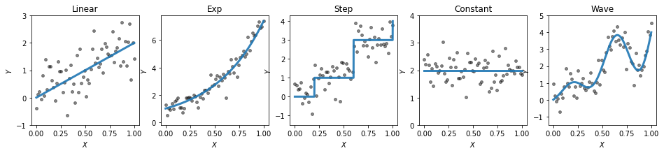
Figure S2: Univariate data generation models. The target functions are depicted by solid curves in blue and instance samples with size $n=64$ are depicted as black dots.

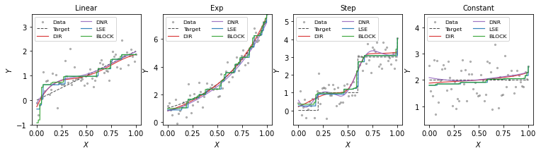
Figure S3: An instance of the estimated curves for the “Linear”, “Exp”, “Step” and “Constant” models when sample size $n=64$. The training data is depicted as grey dots. The target functions are depicted as dashed curves in black, and the estimated functions are depicted by solid curves with different colors.

Table S3: Summary statistics for the simulation results under different univariate models ($d=1$). The averaged mean squared error of the estimates on testing data and $L_{1},L_{2}$ distance to the target function are calculated over 100 replications. The standard deviations are reported in parenthesis.

Model	Method	$n=64$			$n=256$
		MSE	$L_{1}$	$L_{2}$	MSE	$L_{1}$	$L_{2}$
Linear	DNR	0.266 (0.011)	0.101 (0.035)	0.122 (0.040)	0.253 (0.011)	0.055 (0.020)	0.068 (0.023)
	PDIR	0.265 (0.012)	0.098 (0.037)	0.118 (0.041)	0.254 (0.012)	0.058 (0.024)	0.070 (0.027)
	Isotonic LSE	0.282 (0.013)	0.140 (0.027)	0.177 (0.035)	0.262 (0.012)	0.088 (0.012)	0.113 (0.017)
	Block	0.330 (0.137)	0.165 (0.060)	0.243 (0.155)	0.277 (0.033)	0.106 (0.021)	0.153 (0.060)
Exp	DNR	0.268 (0.014)	0.103 (0.043)	0.124 (0.049)	0.256 (0.012)	0.055 (0.024)	0.068 (0.027)
	PDIR	0.268 (0.017)	0.102 (0.049)	0.124 (0.056)	0.255 (0.012)	0.055 (0.022)	0.068 (0.026)
	Isotonic LSE	0.312 (0.018)	0.195 (0.028)	0.246 (0.034)	0.274 (0.014)	0.120 (0.014)	0.153 (0.018)
	Block	0.302 (0.021)	0.177 (0.028)	0.223 (0.034)	0.272 (0.012)	0.115 (0.015)	0.146 (0.017)
Step	DNR	0.375 (0.045)	0.259 (0.059)	0.347 (0.061)	0.315 (0.017)	0.169 (0.022)	0.253 (0.018)
	PDIR	0.366 (0.042)	0.245 (0.058)	0.335 (0.057)	0.311 (0.018)	0.153 (0.025)	0.245 (0.018)
	Isotonic LSE	0.304 (0.020)	0.151 (0.041)	0.228 (0.039)	0.275 (0.014)	0.081 (0.022)	0.155 (0.020)
	Block	0.382 (0.217)	0.208 (0.082)	0.327 (0.160)	0.295 (0.046)	0.108 (0.035)	0.197 (0.086)
Constant	DNR	0.266 (0.012)	0.102 (0.038)	0.122 (0.042)	0.258 (0.013)	0.057 (0.021)	0.069 (0.023)
	PDIR	0.260 (0.011)	0.080 (0.045)	0.092 (0.049)	0.257 (0.012)	0.051 (0.025)	0.060 (0.028)
	Isotonic LSE	0.265 (0.013)	0.087 (0.044)	0.114 (0.052)	0.258 (0.012)	0.044 (0.020)	0.068 (0.025)
	Block	0.264 (0.012)	0.085 (0.044)	0.108 (0.049)	0.258 (0.012)	0.044 (0.020)	0.066 (0.025)
Wave	DNR	0.289 (0.023)	0.156 (0.039)	0.192 (0.044)	0.262 (0.014)	0.089 (0.025)	0.110 (0.029)
	PDIR	0.530 (0.030)	0.398 (0.026)	0.528 (0.018)	0.511 (0.022)	0.368 (0.014)	0.510 (0.009)
	Isotonic LSE	0.525 (0.027)	0.399 (0.022)	0.524 (0.015)	0.495 (0.020)	0.353 (0.009)	0.494 (0.004)
	Block	0.516 (0.024)	0.391 (0.022)	0.519 (0.017)	0.497 (0.023)	0.358 (0.012)	0.500 (0.013)

A.3 Bivariate models

We consider several basic multivariate models, including polynomial model (“Polynomial”), concave model (“Concave”), step model (“Step”), partial model (“Partial”), constant model (“Constant”) and wave model (“Wave”), which correspond to different specifications of the target function $f_{0}$. The formulae are given below.

• Polynomial:

  $$Y=f_{0}(X)+\epsilon=\frac{10}{2^{3/4}}(x_{1}+x_{2})^{3/4}+\epsilon,$$

• Concave:

  $$Y=f_{0}(X)+\epsilon=1+3x_{1}(1-\exp(-3x_{2}))+\epsilon,$$

• Step:

  $$Y=f_{0}(X)+\epsilon=\sum h_{i}I(x_{1}+x_{2}\geq t_{i})+\epsilon,$$

• Partial:

  $$Y=f_{0}(X)+\epsilon=10x_{2}^{8/3}+\epsilon,$$

• Constant:

  $$Y=f_{0}(X)+\epsilon=3+\epsilon,$$

• Wave:

  $$Y=f_{0}(X)+\epsilon=5(x_{1}+x_{2})+3(x_{1}+x_{2})\sin(\pi(x_{1}+x_{2}))+\epsilon,$$

where $X=(x_{1},x_{2})$, $(h_{i})=(1,2,2,1.5,0.5,1)$, $(t_{i})=(0.2,0.6,1.0,1.3,1.7,1.9)$ and $\epsilon\sim N(0,\frac{1}{4})$ follows normal distribution. The “Polynomial” and “Concave” models are monotonic models. The “Step” model is monotonic but not smooth even continuous. In “Partial ” model, the response is related to only one covariate. The “Constant” is a monotonic but not strictly monotonic model and the “Wave” is a nonlinear, smooth but non monotonic model. We use the lattice design for the ease of presentation of Block estimator, where $(X_{i}^{\rm train})_{i=1}^{n}$ are the lattice points evenly distributed on interval $[0,1]^{2}$. Simulation results over 100 replications are summarized in Table S4. And for each model, we take an instance from the replications to present the heatmaps and the 3D surface of the predictions of these estimates; see Figure S4-S15. In heatmaps, we show the observed data (linearly interpolated), the true target function $f_{0}$ and the estimates of different methods. We can see that compared with the piece-wise constant estimates of Isotonic LSE and Block estimator, the DIR estimator is smooth and works reasonably well under bivariate models, especially for models with smooth target functions.

Table S4: Summary statistics for the simulation results under different bivariate models ($d=2$). The averaged mean squared error of the estimates on testing data and $L_{1},L_{2}$ distance to the target function are calculated over 100 replications. The standard deviations are reported in parenthesis.

Model	Method	$n=64$			$n=256$
		MSE	$L_{1}$	$L_{2}$	MSE	$L_{1}$	$L_{2}$
Polynomial	DNR	4.735 (0.344)	0.138 (0.041)	0.172 (0.046)	4.655 (0.178)	0.078 (0.022)	0.098 (0.025)
	PDIR	4.724 (0.366)	0.140 (0.045)	0.171 (0.049)	4.688 (0.181)	0.077 (0.023)	0.096 (0.026)
	Isotonic LSE	8.309 (0.405)	0.755 (0.061)	0.884 (0.061)	6.052 (0.153)	0.364 (0.019)	0.444 (0.021)
	Block	4.780 (0.284)	0.319 (0.020)	0.397 (0.026)	4.747 (0.129)	0.210 (0.011)	0.264 (0.017)
Concave	DNR	0.282 (0.016)	0.142 (0.038)	0.176 (0.042)	0.261 (0.007)	0.083 (0.022)	0.103 (0.024)
	PDIR	0.276 (0.015)	0.129 (0.038)	0.158 (0.043)	0.260 (0.007)	0.077 (0.024)	0.096 (0.028)
	Isotonic LSE	0.393 (0.042)	0.308 (0.051)	0.375 (0.055)	0.294 (0.010)	0.163 (0.020)	0.207 (0.022)
	Block	0.303 (0.015)	0.183 (0.025)	0.229 (0.030)	0.275 (0.006)	0.125 (0.012)	0.157 (0.014)
Step	DNR	0.561 (0.030)	0.462 (0.020)	0.557 (0.025)	0.519 (0.011)	0.432 (0.010)	0.519 (0.010)
	PDIR	0.561 (0.030)	0.461 (0.019)	0.557 (0.024)	0.519 (0.011)	0.431 (0.010)	0.520 (0.010)
	Isotonic LSE	1.462 (0.104)	0.852 (0.046)	1.100 (0.047)	0.700 (0.028)	0.430 (0.019)	0.672 (0.021)
	Block	0.657 (0.031)	0.503 (0.022)	0.638 (0.023)	0.461 (0.016)	0.321 (0.014)	0.457 (0.014)
Partial	DNR	12.67 (0.530)	0.129 (0.033)	0.161 (0.039)	12.77 (0.338)	0.079 (0.023)	0.099 (0.027)
	PDIR	12.70 (0.548)	0.112 (0.037)	0.136 (0.042)	12.72 (0.285)	0.063 (0.021)	0.080 (0.026)
	Isotonic LSE	17.78 (0.532)	0.739 (0.052)	1.062 (0.055)	15.00 (0.262)	0.378 (0.024)	0.528 (0.028)
	Block	12.31 (0.571)	0.435 (0.041)	0.578 (0.043)	12.50 (0.313)	0.237 (0.028)	0.313 (0.049)
Constant	DNR	0.278 (0.016)	0.131 (0.038)	0.160 (0.042)	0.260 (0.005)	0.079 (0.020)	0.097 (0.022)
	PDIR	0.266 (0.013)	0.094 (0.047)	0.111 (0.050)	0.255 (0.005)	0.052 (0.022)	0.063 (0.025)
	Isotonic LSE	0.280 (0.021)	0.121 (0.047)	0.161 (0.056)	0.262 (0.006)	0.076 (0.025)	0.108 (0.026)
	Block	0.265 (0.012)	0.089 (0.040)	0.110 (0.046)	0.256 (0.005)	0.059 (0.022)	0.075 (0.024)
Wave	DNR	0.306 (0.020)	0.189 (0.036)	0.233 (0.042)	0.269 (0.009)	0.108 (0.025)	0.135 (0.029)
	PDIR	0.459 (0.058)	0.390 (0.056)	0.454 (0.063)	0.581 (0.039)	0.493 (0.028)	0.574 (0.033)
	Isotonic LSE	1.380 (0.085)	0.918 (0.032)	1.063 (0.040)	0.989 (0.024)	0.760 (0.014)	0.860 (0.012)
	Block	0.978 (0.022)	0.750 (0.014)	0.854 (0.012)	0.892 (0.021)	0.693 (0.009)	0.802 (0.008)

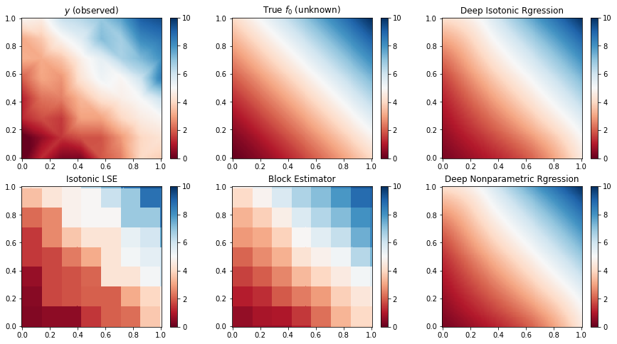
Figure S4: Heatmaps for the target function $f_{0}$, the observed training data, and its deep isotonic regression and isotonic least squares estimate (isotonic LSE) under model (a) when $d=2$ and $n=64$.

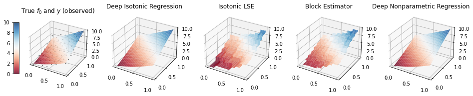
Figure S5: 3D surface plots for the target function $f_{0}$, the observed training data, and its deep isotonic regression and isotonic least squares estimate (isotonic LSE) under model (a) when $d=2$ and $n=64$.

Figure S6: Heatmaps for the target function $f_{0}$, the observed training data, and its deep isotonic regression and isotonic least squares estimate (isotonic LSE) under model (b) when $d=2$ and $n=64$.

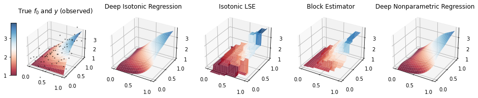
Figure S7: 3D surface plots for the target function $f_{0}$, the observed training data, and its deep isotonic regression and isotonic least squares estimate (isotonic LSE) under model (b) when $d=2$ and $n=64$.

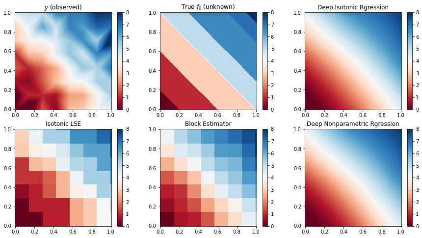
Figure S8: Heatmaps for the target function $f_{0}$, the observed training data, and its deep isotonic regression and isotonic least squares estimate (isotonic LSE) under model (c) when $d=2$ and $n=64$.

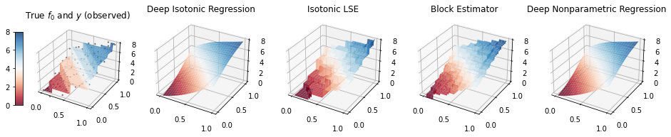
Figure S9: 3D surface plots for the target function $f_{0}$, the observed training data, and its deep isotonic regression and isotonic least squares estimate (isotonic LSE) under model (c) when $d=2$ and $n=64$.

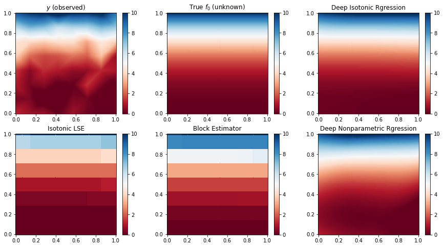
Figure S10: Heatmaps for the target function $f_{0}$, the observed training data, and its deep isotonic regression and isotonic least squares estimate (isotonic LSE) under model (d) when $d=2$ and $n=64$.

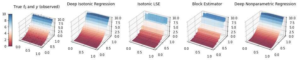
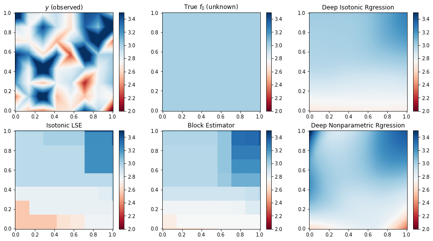
Figure S11: 3D surface plots for the target function $f_{0}$, the observed training data, and its deep isotonic regression and isotonic least squares estimate (isotonic LSE) under model (d) when $d=2$ and $n=64$.

Figure S12: Heatmaps for the target function $f_{0}$, the observed training data, and its deep isotonic regression and isotonic least squares estimate (isotonic LSE) under model (e) when $d=2$ and $n=64$.

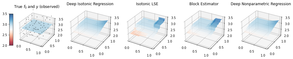
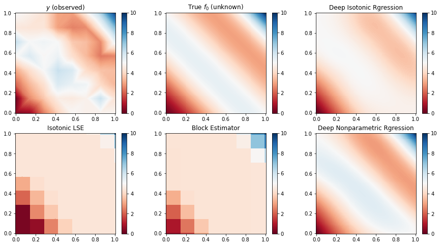
Figure S13: 3D surface plots for the target function $f_{0}$, the observed training data, and its deep isotonic regression and isotonic least squares estimate (isotonic LSE) under model (e) when $d=2$ and $n=64$.

Figure S14: Heatmaps for the target function $f_{0}$, the observed training data, and its deep isotonic regression and isotonic least squares estimate (isotonic LSE) under model (f) when $d=2$ and $n=64$.

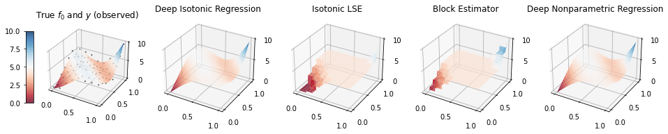
Figure S15: 3D surface plots for the target function $f_{0}$, the observed training data, and its deep isotonic regression and isotonic least squares estimate (isotonic LSE) under model (f) when $d=2$ and $n=64$.

A.4 Tuning parameter

In this subsection, we investigate the numerical performance regrading to different choice of tuning parameters under different models.

For univariate models, we calculate the testing statistics $L_{1}$ and $L_{2}$ for tuning parameter $\lambda$ on the 20 lattice points in the interval $[0,3\log(n)]$. For each $\lambda$, we simulate 20 times replications and reports the average $L_{1}$, $L_{2}$ statistics and their 90% empirical band. For each replication, we train the PDIR using $n=256$ training samples and $T=1,000$ testing samples. In our simulation, four univariate models in section A.2 are considered including “Exp”, “Constant”, “Step” and misspecified model “Wave” and the results are reported in Figure S16. We can see that for isotonic models “Exp” and “Step”, the estimate is not sensitive to the choice of the tuning parameter $\lambda$ in $[0,3\log(n)]$, which all leads to reasonable estimates. For “Constant” model, a not strictly isotonic model, errors slightly increase as the tuning parameter $\lambda$ increases in $[0,3\log(n)]$. Overall, the choice $\lambda=\log(n)$ can lead to reasonably well estimates for correctly specified models. For misspecified model “Wave”, the estimates deteriorates quickly as the tuning parameter $\lambda$ increases around 0, and after that the additional negative effect of the increasing $\lambda$ becomes slight.

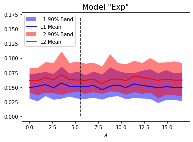
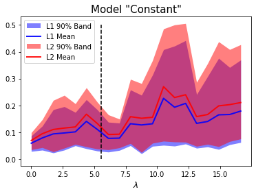
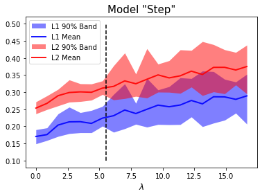
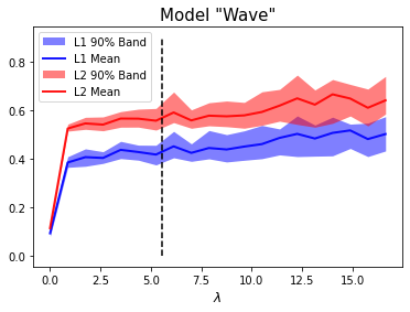
Figure S16: $L_{1}$ and $L_{2}$ distances between estimates and the targets with different tuning parameters under univariate models with size $n=256$. For each value of tuning parameter $\lambda$, the mean $L_{1}$ and $L_{2}$ distances (solid blue and red curves) and their 90% empirical band (blue and red ranges) are calculated over 20 replications. A vertical dashed line is presented at $\lambda=\log(n)$.

For bivariate models, our first simulation studies focus on the case where tuning parameters have the same value, i.e., $\lambda_{1}=\lambda_{2}$. We calculate the testing statistics $L_{1}$ and $L_{2}$ for tuning parameters $\lambda_{1}=\lambda_{2}$ on the 20 lattice points in the interval $[0,3\log(n)]$. For each $\lambda$, we simulate 20 times replications and reports the average $L_{1}$, $L_{2}$ statistics and their 90% empirical band. For each replication, we train the PDIR using $n=256$ training samples and $T=10,000$ testing samples. In our simulation, four bivariate models in section A.3 are considered including “Partial”, “Constant”, “Concave” and misspecified model “Wave” and the results are reported in Figure S17. The observation are similar to those of univariate models, that is, the estimates are not sensitive to the choices of tuning parameters over $[0,3\log(n)]$ for correctly specified models, i.e., isotonic models. But for misspecified model “Wave”, the estimates deteriorates quickly as the tuning parameter $\lambda$ increases around 0, and after that increasing $\lambda$ slightly spoils the estimates.

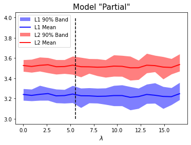
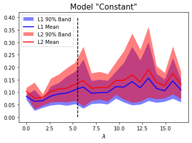
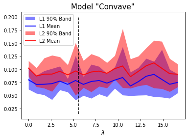
Figure S17: $L_{1}$ and $L_{2}$ distances between estimates and the targets with different tuning parameters under bivariate models with size $n=256$. For each value of tuning parameter $(\lambda_{1},\lambda_{2})$ with $\lambda_{1}=\lambda_{2}$, the mean $L_{1}$ and $L_{2}$ distances (solid blue and red curves) and their 90% empirical band (blue and red ranges) are calculated over 20 replications. A vertical dashed line is presented at $\lambda_{1}=\lambda_{2}=\log(n)$.

In the second simulation study of bivariate models, we can choose different values for different components of the turning parameter $\lambda=(\lambda_{1},\lambda_{2})$, i.e., $\lambda_{1}$ can be different from $\lambda_{2}$. We investigate this by considering the follow bivariate model, where the target function $f_{0}$ is monotonic in its second argument and non-monotonic in its first one.

• :

  $$Y=f_{0}(X)+\epsilon=2\sin(2\pi x_{1})+4(x_{2})^{4/3}+\epsilon,$$

where $X=(x_{1},x_{2})$ and $\epsilon\sim N(0,\frac{1}{4})$ follows normal distribution. Heatmaps for the observed training data, the target function $f_{0}$, and 3D surface plots for the target function $f_{0}$ under model (g) when $d=2$ and $n=256$ are presented in Figure S18.

For model (g), we calculate the mean testing statistics $L_{1}$ and $L_{2}$ for tuning parameter $\lambda=(\lambda_{1},\lambda_{2})$ on the 400 grid points on the region $[0,3\log(n)]\times[0,3\log(n)]$. For each $\lambda=(\lambda_{1},\lambda_{2})$, we simulate 5 times replications and reports the average $L_{1}$, $L_{2}$ statistics. For each replication, we train the PDIR using $n=256$ training samples and $T=10,000$ testing samples. The mean $L_{1}$ and $L_{2}$ distance from the target function and the estimates on the testing data under different $\lambda$ are depicted in Figure S19. We see that the target function $f_{0}$ is increasing in its second argument, and the estimates is insensitive to the tuning parameter $\lambda_{2}$, while the target function $f_{0}$ is non-monotonic in its first argument, and the estimates deteriorate when $\lambda_{1}$ gets larger. The simulation results suggest that we should only penalize the gradient with respect to the monotonic arguments but not non-monotonic ones. The estimates is sensitive to the turning parameter for misspecified model, especially when the turning parameter increases around $0$.

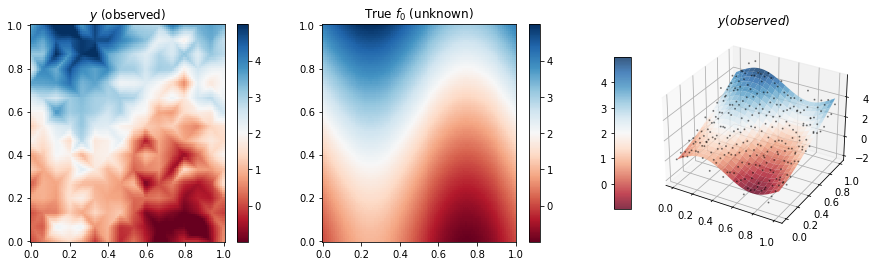
Figure S18: Heatmaps for the observed training data, the target function $f_{0}$, and 3D surface plots for the target function $f_{0}$ under model (g) when $d=2$ and $n=256$.

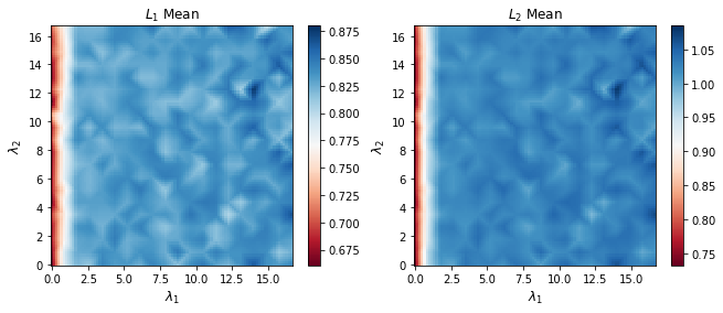
Figure S19: Heatmaps for the observed training data, the target function $f_{0}$, and 3D surface plots for the target function $f_{0}$ under model (g) when $d=2$ and $n=256$.

Appendix B Proofs

Proof of Theorem 1

Let $p$ be an integer greater than or equal to 2. We define the RePU activation functions $\sigma_{p-1}(x)=\max{0,x}^{p-1}$ and $\sigma_{p}(x)=\max\{0,x^{p}\}$. We use $(d_{0},d_{1},\ldots,d_{\mathcal{D}+1})$ to denote the width (number of neurons) of each layer in the original RePU network, where $d_{0}=d$ and $d_{\mathcal{D}+1}=1$ in our problem. For $u=1,\ldots,d_{i}$ and $i=1,\ldots,\mathcal{D}+1$, we let $f^{(i)}_{u}$ denote the function that takes an input $X=(x_{1},\ldots,x_{d})\in\mathcal{X}\subset\mathbb{R}^{d}$ and outputs the $u$-th neuron of the $i$-th layer. To compute $(\frac{\partial}{\partial x_{j}}f^{(i)}_{1},\ldots,\frac{\partial}{\partial x_{j}}f^{(i)}_{d_{i}})$ iteratively for $i=1,\ldots,\mathcal{D}+1$, we construct a series of Mixed RePUs activated subnetworks, which are used to compute the partial derivatives of the original RePU networks (up to the $i$-th layer) step by step. Without loss of generality, we compute $(\frac{\partial}{\partial x_{j}}f^{(i)}_{1},\ldots,\frac{\partial}{\partial x_{j}}f^{(i)}_{d_{i}})$ for $j\in{1,\ldots,d}$ in our proof. We present the construction details of the Mixed RePUs sub-networks in three steps. In the first and second step, we show how to construct Mixed RePUs subnetworks to compute $(\frac{\partial}{\partial x_{j}}f^{(i)}_{1},\ldots,\frac{\partial}{\partial x_{j}}f^{(i)}_{d_{i}})$ for the first two layers ($i=1,2$). Then for intermediate layers $i=3,\ldots,\mathcal{D}$ we can apply induction. Lastly, we show construction for the last layer ($i=\mathcal{D}+1$).

Step 1. Recall that the derivative of $\sigma_{p}$ is $\sigma^{\prime}_{p}(x)=p\sigma_{p-1}(x)$. When $i=1$ and $u=1,\ldots,d_{1}$, we have

$$\frac{\partial}{\partial x_{j}}f^{(1)}_{u}=\frac{\partial}{\partial x_{j}}\sigma_{p}\Big{(}\sum_{i=1}^{d_{0}}w^{(1)}_{ui}x_{i}+b_{u}^{(1)}\Big{)}=p\sigma_{p-1}\Big{(}\sum_{i=1}^{d_{0}}w^{(1)}_{ui}x_{i}+b_{u}^{(1)}\Big{)}\cdot w_{u,d_{0}}^{(1)},$$ (B.1)

where we denote $w^{(1)}_{ui}$ and $b_{u}^{(1)}$ by the corresponding weights and bias in $1$-th layer of the original RePU network. In the following, we build a network taking $X=(x_{1},\ldots,x{d_{0}})$ as input and outputs

$$(f^{(1)}_{1},\ldots,f^{(1)}_{d_{1}},\frac{\partial}{\partial x_{j}}f^{(1)}_{1},\ldots,\frac{\partial}{\partial x_{j}}f^{(1)}_{d_{1}})\in\mathbb{R}^{2d_{1}}.$$

The constructed network has 4-layer and width $(d_{0},3d_{1},10d_{1},2d_{1})$. And it worth noting that such network will output all necessary items to compute $(\frac{\partial}{\partial x_{j}}f^{(2)}_{1},\ldots,\frac{\partial}{\partial x_{j}}f^{(2)}_{d_{2}})$. In the first hidden layer of the constructed network, we can obtain $3d_{1}$ neurons

$$(f^{(1)}_{1},\ldots,f^{(1)}_{d_{1}},p|w^{(1)}_{1,d_{0}}|,\ldots,p|w^{(1)}_{d_{1},d_{0}}|,\sigma_{p-1}(\sum_{i=1}^{d_{0}}w^{(1)}_{1i}x_{i}+b^{(1)}_{1}),\ldots,\sigma_{p-1}(\sum_{i=1}^{d_{0}}w^{(1)}_{d_{1}i}x_{i}+b^{(1)}_{d_{1}})),$$

where $B^{(1)}_{1}$ is the bias vector, $\Sigma_{1}$ is a vector of activations, and the weight matrix $A^{(1)}_{1}$ has$2d_{0}d_{1}$ parameters. The $A^{(1)}_{1},B^{(1)}_{1}$ and $\Sigma_{1}$ are specified by

$$A^{(1)}_{1}=\left[\begin{array}[]{ccccc}w^{(1)}_{1,1}&w^{(1)}_{1,2}&\cdots&\cdots&w^{(1)}_{1,d_{0}}\\ w^{(1)}_{2,1}&w^{(1)}_{2,2}&\cdots&\cdots&w^{(1)}_{2,d_{0}}\\ \ldots&\ldots&\ldots&\ldots&\ldots\\ w^{(1)}_{d_{1},1}&w^{(1)}_{d_{1},2}&\cdots&\cdots&w^{(1)}_{d_{1},d_{0}}\\ 0&0&0&0&0\\ \ldots&\ldots&\ldots&\ldots&\ldots\\ 0&0&0&0&0\\ w^{(1)}_{1,1}&w^{(1)}_{1,2}&\cdots&\cdots&w^{(1)}_{1,d_{0}}\\ w^{(1)}_{2,1}&w^{(1)}_{2,2}&\cdots&\cdots&w^{(1)}_{2,d_{0}}\\ \ldots&\ldots&\ldots&\ldots&\ldots\\ w^{(1)}_{d_{1},1}&w^{(1)}_{d_{1},2}&\cdots&\cdots&w^{(1)}_{d_{1},d_{0}}\\ \end{array}\right]\in\mathbb{R}^{3d_{1}\times d_{0}},\quad B^{(1)}_{1}=\left[\begin{array}[]{c}b^{(1)}_{1}\\ b^{(1)}_{2}\\ \ldots\\ b^{(1)}_{d_{1}}\\ p|w^{(1)}_{1,d_{0}}|\\ p|w^{(1)}_{2,d_{0}}|\\ \ldots\\ p|w^{(1)}_{d_{1},d_{0}}|\\ b^{(1)}_{1}\\ b^{(1)}_{2}\\ \ldots\\ b^{(1)}_{d_{1}}\\ \end{array}\right]\in\mathbb{R}^{3d_{1}},\quad\Sigma^{(1)}_{1}=\left[\begin{array}[]{c}\sigma_{p}\\ \ldots\\ \sigma_{p}\\ \sigma_{1}\\ \ldots\\ \sigma_{1}\\ \sigma_{p-1}\\ \ldots\\ \sigma_{p-1}\\ \end{array}\right],$$

where the first $d_{1}$ activation functions of $\Sigma_{1}$ are chosen to be $\sigma_{p}$, the last $d_{1}$ activation functions are chosen to be $\sigma_{p-1}$ and the rest are $\sigma_{1}$.

Consequently, the second hidden layer has $6d_{1}$ computing units (neurons). The first $2d_{1}$ neurons are designed to compute an identity mapping such that $(f^{(1)}1,\ldots,f^{(1)}{d_{1}})$ can be kept in the next layer. These neurons take the form of

$$(\sigma_{1}(f^{(1)}_{1}),\sigma_{1}(-f^{(1)}_{1})),\ldots,\sigma_{1}(f^{(1)}_{d_{1}}),\sigma_{1}(-f^{(1)}_{d_{1}})),$$

where the identity mapping can be represented by $x=\sigma_{1}(x)-\sigma_{1}(-x)$ using ReLU layer. Based on the fact that

$$x\cdot y=\frac{1}{4}\{\sigma_{2}(x+y)+\sigma_{2}(-x-y)-\sigma_{2}(x-y)-\sigma_{2}(-x+y)\},$$

the remaining $4d_{1}$ neurons in the second hidden layer are used for performing the nonlinear multiplications in (B.1) to obtain $(\frac{\partial}{\partial x_{j}}f^{(1)}_{1},\ldots,\frac{\partial}{\partial x_{j}}f^{(1)}_{d_{1}})\in\mathbb{R}^{d_{1}}$. The remaining $4d_{1}$ neurons are

$$\left[\begin{array}[]{c}\sigma_{2}(p\cdot w^{(1)}_{1,d_{0}}+\sigma_{p-1}(\sum_{i=1}^{d_{0}}w^{(1)}_{1i}x_{i}+b^{(1)}_{1}))\\ \sigma_{2}(p\cdot w^{(1)}_{1,d_{0}}-\sigma_{p-1}(\sum_{i=1}^{d_{0}}w^{(1)}_{1i}x_{i}+b^{(1)}_{1}))\\ \sigma_{2}(-p\cdot w^{(1)}_{1,d_{0}}+\sigma_{p-1}(\sum_{i=1}^{d_{0}}w^{(1)}_{1i}x_{i}+b^{(1)}_{1})\\ \sigma_{2}(-p\cdot w^{(1)}_{1,d_{0}}-\sigma_{p-1}(\sum_{i=1}^{d_{0}}w^{(1)}_{1i}x_{i}+b^{(1)}_{1}))\\ \ldots\\ \sigma_{2}(p\cdot w^{(1)}_{d_{1},d_{0}}+\sigma_{p-1}(\sum_{i=1}^{d_{0}}w^{(1)}_{d_{1}i}x_{i}+b^{(1)}_{d_{1}}))\\ \sigma_{2}(p\cdot w^{(1)}_{d_{1},d_{0}}-\sigma_{p-1}(\sum_{i=1}^{d_{0}}w^{(1)}_{d_{1}i}x_{i}+b^{(1)}_{d_{1}}))\\ \sigma_{2}(-p\cdot w^{(1)}_{d_{1},d_{0}}+\sigma_{p-1}(\sum_{i=1}^{d_{0}}w^{(1)}_{d_{1}i}x_{i}+b^{(1)}_{d_{1}})\\ \sigma_{2}(-p\cdot w^{(1)}_{d_{1},d_{0}}-\sigma_{p-1}(\sum_{i=1}^{d_{0}}w^{(1)}_{d_{1}i}x_{i}+b^{(1)}_{d_{1}}))\\ \end{array}\right]\in\mathbb{R}^{4d_{1}}.$$

Here the bias vector is zero $B^{(1)}_{2}=(0,\ldots,0)\in\mathbb{R}^{6d_{1}}$, and activation functions vector is

$$\Sigma^{(1)}_{2}=(\underbrace{\sigma_{1},\ldots,\sigma_{1}}_{2d_{1}\ {\rm times}},\underbrace{\sigma_{2},\ldots,\sigma_{2}}_{4d_{1}\ {\rm times}})$$

for the second hidden layer.

The weight matrix $A^{(1)}_{2}$ in the second hidden layer can be specified accordingly, containing $2d_{1}+8d_{1}=10d_{1}$ non-zero parameters. Lastly, we utilize identity mappings and multiplication operations with weight matrix $A^{(1)}_{3}$ (containing $2d_{1}+4d_{1}=6d_{1}$ parameters) and a zero bias vector $B^{(1)}_{3}$ to get

$$(f^{(1)}_{1},\ldots,f^{(1)}_{d_{1}},\frac{\partial}{\partial x_{j}}f^{(1)}_{1},\ldots,\frac{\partial}{\partial x_{j}}f^{(1)}_{d_{1}})\in\mathbb{R}^{2d_{1}},$$

which compute the last layer.

The resulting Mixed RePUs activated network has a architecture specified by two hidden layers, $11d_{1}$ hidden neurons, $2d_{0}d_{1}+3d_{1}+10d_{1}+6d_{1}=2d_{0}d_{1}+19d_{1}$ parameters, and a width of $(d_{0},3d_{1},6d_{1},2d_{1})$. It is important to see that the activation functions are not suitable for the last layer. When concatenating two consecutive sub-networks into one deep neural network, the activation functions should be implemented to the output of the first network. Therefore, to build the final deep network, the sub-network here would output $4d_{1}$ neurons

$$(\sigma_{1}(f^{(1)}_{1}),\sigma_{1}(-f^{(1)}_{1})\ldots,\sigma_{1}(f^{(1)}_{d_{1}}),\sigma_{1}(-f^{(1)}_{d_{1}}),$$

$$\qquad\sigma_{1}(\frac{\partial}{\partial x_{j}}f^{(1)}_{1}),\sigma_{1}(-\frac{\partial}{\partial x_{j}}f^{(1)}_{1})\ldots,\sigma_{1}(\frac{\partial}{\partial x_{j}}f^{(1)}_{d_{1}}),\sigma_{1}(-\frac{\partial}{\partial x_{j}}f^{(1)}_{d_{1}}))\in\mathbb{R}^{4d_{1}},$$

to keep $(f^{(1)}_{1},\ldots,f^{(1)}_{d_{1}},\frac{\partial}{\partial x_{j}}f^{(1)}_{1},\ldots,\frac{\partial}{\partial x_{j}}f^{(1)}_{d_{1}})$ for the usefulness in the next sub-network. For the constructed network here, the weight matrix $A^{(1)}_{3}$ has $2d_{1}+8d_{1}=10d_{1}$ parameters, the bias vector $B^{(1)}_{3}$ is zero, and all components of $\Sigma^{(1)}_{3}$ are $\sigma_{1}$. This Mixed RePUs neural network has two hidden layers, $13d_{1}$ hidden neurons, $2d_{0}d_{1}+3d_{1}+10d_{1}+10d_{1}=2d_{0}d_{1}+23d_{1}$ parameters, and a width of $(d_{0},3d_{1},6d_{1},4d_{1})$.

Step 2. For any $u=1,\ldots,d_{2}$,

$$\frac{\partial}{\partial x_{j}}f^{(2)}_{u} =\frac{\partial}{\partial x_{j}}\sigma_{p}\Big{(}\sum_{i=1}^{d_{1}}w^{(2)}_{ui}f^{(1)}_{i}+b_{u}^{(2)}\Big{)}$$

$$=p\sigma_{p-1}\Big{(}\sum_{i=1}^{d_{1}}w^{(2)}_{ui}f^{(1)}_{i}+b_{u}^{(2)}\Big{)}\cdot\sum_{i=1}^{d_{1}}w_{u,i}^{(2)}\frac{\partial}{\partial x_{j}}f^{(1)}_{i},$$ (B.2)

where we denote $w^{(2)}_{ui}$ and $b_{u}^{(2)}$ by the weights and bias in the second layer of the original RePU network. Recall that the output of the previously built network in step 1, is the input in our construced network here. In the first hidden layer, we can compute $3d_{2}$ neurons as

$$\Big{(}f^{(2)}_{1},\ldots,f^{(2)}_{d_{2}},|\sum_{i=1}^{d_{1}}w_{1,i}^{(2)}\frac{\partial}{\partial x_{j}}f^{(1)}_{i}|,\ldots,|\sum_{i=1}^{d_{1}}w_{d_{2},i}^{(2)}\frac{\partial}{\partial x_{j}}f^{(1)}_{i}|,$$

$$\qquad\qquad\sigma_{p-1}(\sum_{i=1}^{d_{1}}w^{(2)}_{1i}f^{(1)}_{i}+b^{(1)}_{1}),\ldots,\sigma_{p-1}(\sum_{i=1}^{d_{1}}w^{(2)}_{d_{2}i}f^{(1)}_{i}+b^{(2)}_{d_{2}})\Big{)}.$$

Corresponding to the first hidden layer, the weight matrix $A^{(2)}_{1}\in\mathbb{R}^{3d_{2}\times 4d_{1}}$ has $6d_{1}d_{2}$ non-zero parameters, bias vector $B^{(2)}_{1}\in\mathbb{R}^{3d_{2}}$ and the vector of activations $\Sigma^{(2)}_{1}=\Sigma^{(1)}_{1}$.

As the construction in Step 1, the second hidden layer can be designed to compute $6d_{2}$ neurons, with a weight matrix $A^{(2)}_{2}\in\mathbb{R}^{3d_{2}\times 6d_{2}}$ containing $2d_{2}+8d_{2}=10d_{2}$ non-zero parameters, a zero bias vector $B^{(2)}_{1}\in\mathbb{R}^{6d_{2}}$, and an activation function vector $\Sigma^{(2)}_{2}=\Sigma^{(1)}_{2}$. The second hidden layer serves the same purpose as that in Step 1, which computes the identity mapping for $(f^{(2)}_{1},\ldots,f^{(2)}_{d_{2}})$ and the multiplication in (B.2). Again, the design of the last layer can also follow that in Step 1. The last layer computes

$$(\sigma_{1}(f^{(2)}_{1}),\sigma_{1}(-f^{(2)}_{1})\ldots,\sigma_{1}(f^{(2)}_{d_{2}}),\sigma_{1}(-f^{(2)}_{d_{2}}),$$

$$\qquad\sigma_{1}(\frac{\partial}{\partial x_{j}}f^{(2)}_{1}),\sigma_{1}(-\frac{\partial}{\partial x_{j}}f^{(2)}_{1})\ldots,\sigma_{1}(\frac{\partial}{\partial x_{j}}f^{(2)}_{d_{2}}),\sigma_{1}(-\frac{\partial}{\partial x_{j}}f^{(2)}_{d_{2}}))\in\mathbb{R}^{4d_{2}},$$

with a weight matrix $A^{(2)}_{3}$ containing $2d_{2}+8d_{2}=10d_{2}$ parameters, a zero bias vector $B^{(2)}_{3}$, and an activation function vector $\Sigma^{(1)}_{3}$ whose components are $\sigma_{1}$. Finally, with 17d2 hidden neurons, the second subnetwork of Mixed RePUs comprises 4 layers and $6d_{1}d_{2}+23d_{2}$ parameters. Its width is given by $(4d_{1},3d_{2},6d_{2},4d_{2})$.

Step 3. The process of building Mixed RePUs networks can be continued for integers $k=3,\ldots,\mathcal{D}$ and any $u=1,\ldots,d_{k}$ to compute

$$\frac{\partial}{\partial x_{j}}f^{(k)}_{u} =\frac{\partial}{\partial x_{j}}\sigma_{p}\Big{(}\sum_{i=1}^{d_{k-1}}w^{(k)}_{ui}f^{(k-1)}_{i}+b_{u}^{(k)}\Big{)}$$

$$=p\sigma_{p-1}\Big{(}\sum_{i=1}^{d_{k-1}}w^{(k)}_{ui}f^{(k-1)}_{i}+b_{u}^{(k)}\Big{)}\cdot\sum_{i=1}^{d_{k-1}}w_{u,i}^{(k)}\frac{\partial}{\partial x_{j}}f^{(k-1)}_{i},$$

where $w^{(k)}_{ui}$ and $b_{u}^{(k)}$ are the weights and bias in $k$-th layer of the original RePU network. These designed Mixed RePUs networks receive inputs from the previous one, where the inputs are

$$(\sigma_{1}(f^{(k-1)}_{1}),\sigma_{1}(-f^{(k-1)}_{1})\ldots,\sigma_{1}(f^{(k-1)}_{d_{k-1}}),\sigma_{1}(-f^{(k-1)}_{d_{k-1}}),$$

$$\qquad\sigma_{1}(\frac{\partial}{\partial x_{j}}f^{(k-1)}_{1}),\sigma_{1}(-\frac{\partial}{\partial x_{j}}f^{(k-1)}_{1})\ldots,\sigma_{1}(\frac{\partial}{\partial x_{j}}f^{(k-1)}_{d_{k-1}}),\sigma_{1}(-\frac{\partial}{\partial x_{j}}f^{(k-1)}_{d_{k-1}}))\in\mathbb{R}^{4d_{k-1}}.$$

And these Mixed RePUs networks output

$$(\sigma_{1}(f^{(k)}_{1}),\sigma_{1}(-f^{(k)}_{1})\ldots,\sigma_{1}(f^{(k)}_{d_{k}}),\sigma_{1}(-f^{(k)}_{d_{k}}),$$

$$\qquad\sigma_{1}(\frac{\partial}{\partial x_{j}}f^{(k)}_{1}),\sigma_{1}(-\frac{\partial}{\partial x_{j}}f^{(k)}_{1})\ldots,\sigma_{1}(\frac{\partial}{\partial x_{j}}f^{(k)}_{d_{k}}),\sigma_{1}(-\frac{\partial}{\partial x_{j}}f^{(k)}_{d_{k}}))\in\mathbb{R}^{4d_{k}}.$$

Correspondingly, the architecture of these Mixed RePUs networks is specified with two hidden layers, $13d_{k}$ hidden neurons, $6d_{k-1}d_{k}+23d_{k}$ parameters. Their width is given by $(4d_{k-1},3d_{k},6d_{k},4d_{k})$.

The aforementioned process can be replicated until the $k=\mathcal{D}+1$ stage, at which point the final layer (i.e., $\mathcal{D}+2$ layer) of the original RePU network outputs one-dimensional scale instead of $4d_{k}$-dimensional vector in step $k=1,\ldots,\mathcal{D}$. Consequently, the design requires some modifications.

As a reminder, for a RePU-activated neural network $f\in\mathcal{F}_{n}=\mathcal{F}_{\mathcal{D},\mathcal{W},\mathcal{U},\mathcal{S},\mathcal{B}}$, its partial derivative with respect to $x_{j}$ is given by

$$\frac{\partial}{\partial x_{j}}f=\frac{\partial}{\partial x_{j}}\sum_{i=1}^{d_{\mathcal{D}}}w^{(\mathcal{D})}_{i}f^{(\mathcal{D})}_{i}+b^{(\mathcal{D})}=\sum_{i=1}^{d_{\mathcal{D}}}w^{(\mathcal{D})}_{i}\frac{\partial}{\partial x_{j}}f^{(\mathcal{D})}_{i}.$$

In addition, the Mixed RePU network in step $\mathcal{D}$ outputs

$$(\sigma_{1}(f^{(\mathcal{D})}_{1}),\sigma_{1}(-f^{(\mathcal{D})}_{1})\ldots,\sigma_{1}(f^{(\mathcal{D})}_{d_{\mathcal{D}}}),\sigma_{1}(-f^{(\mathcal{D})}_{d_{\mathcal{D}}}),$$

$$\qquad\sigma_{1}(\frac{\partial}{\partial x_{j}}f^{(\mathcal{D})}_{1}),\sigma_{1}(-\frac{\partial}{\partial x_{j}}f^{(\mathcal{D})}_{1})\ldots,\sigma_{1}(\frac{\partial}{\partial x_{j}}f^{(\mathcal{D})}_{d_{\mathcal{D}}}),\sigma_{1}(-\frac{\partial}{\partial x_{j}}f^{(\mathcal{D})}_{d_{\mathcal{D}}}))\in\mathbb{R}^{4d_{\mathcal{D}}},$$

which will be the input of the network in step $\mathcal{D}+1$ here. The objective of the network is to calculate $\frac{\partial}{\partial x_{j}}f^{(\mathcal{D}+1)}=\frac{\partial}{\partial x_{j}}f$, which represents the partial derivative of the original RePU network with respect to its $j$-th argument $x_{j}$. With minor modification, it is not hard to see that the network architecture should feature two hidden layers with a width of $(4d_{\mathcal{D}},2,8,1)$, 11 hidden neurons, and $4d_{\mathcal{D}}+2+16=4d_{\mathcal{D}}+18$ non-zero parameters.

In the end, we composite all $\mathcal{D}+1$ networks to create a Mixed RePUs network, which accepts an input $X=(x_{1},\ldots,x_{d})\in\mathbb{R}^{d}$ and produces $\frac{\partial}{\partial x_{j}}f$ for $f\in\mathcal{F}_{n}=\mathcal{F}{\mathcal{D},\mathcal{W},\mathcal{U},\mathcal{S},\mathcal{B},\mathcal{B}^{\prime}}$. Consequently, the Mixed RePUs network has $3\mathcal{D}+3$ hidden layers, $d_{0}+\sum_{i=1}^{\mathcal{D}}13d_{i}+11\leq 13\mathcal{U}$ neurons, $2d_{0}d_{1}+23d_{1}+\sum_{i=1}^{\mathcal{D}}(6d_{i}d_{i+1}+23d_{i+1})+4d_{\mathcal{D}}+18\leq 23\mathcal{S}$ parameters, and a width of $6\max{d_{1},\ldots,d_{\mathcal{D}}}=6\mathcal{W}$. This completes the proof. $\hfill\Box$

Proof of Lemma 1

We aim to establish an upper bound on the Pseudo dimension of $\mathcal{F}$ which is expressed in the parameters of the network architecture, i.e., depth, size, and number of neurons. This bound is stronger than the VC dimension of ${\rm sign}(\mathcal{F})$, as shown by the inequality ${\rm VCdim}({\rm sign}(\mathcal{F}))\leq{\rm Pdim}(\mathcal{F})$ in Bartlett et al. (2019).

Our proof builds upon the approach presented in Lemma 4 of Shen et al. (2022) and Theorem 6 of Bartlett et al. (2019). While we briefly describe the main step underlying our proof, we recommend interested readers to refer to Lemma 4 of Shen et al. (2022) and Theorem 6 of Bartlett et al. (2019) for detailed exposition.

Step 1. Consider a new class of functions $\tilde{\mathcal{F}}:=\{\tilde{f}(z,t)={\rm sign}(f(z)-t):f\in\mathcal{F}\}.$ We aim to bound the VC dimension of $\tilde{\mathcal{F}}$ since ${\rm Pdim}(\mathcal{F})\leq{\rm VCdim}(\tilde{\mathcal{F}})$. Let $\theta\in\mathbb{R}^{\mathcal{S}}$ denote the parameters vector of the network $f(\cdot,\theta):\mathcal{Z}\to\mathbb{R}$ implemented in $\mathcal{F}$. We derive a bound for

$$K(m):=\Big{|}\{({\rm sign}(f(z_{1},\theta)-t_{1}),\ldots,{\rm sign}(f(z_{m},\theta)-t_{m})):\theta\in\mathbb{R}^{\mathcal{S}}\}\Big{|}$$

which uniformly holds for all choice of $\{z_{i}\}_{i=1}^{m}$ and $\{t_{i}\}_{i=1}^{m}$.

Step 2. We find a partition $\mathcal{P}=\{P_{1},\ldots,P_{N}\}$ of the domain $\mathbb{R}^{\mathcal{S}}$ such that within each region $P_{i}$, the functions $f(z_{j},\cdot)$ are all fixed polynomials of bounded degree. Then $K(m)$ is bounded via

$$K(m)\leq\sum_{i=1}^{N}\Big{|}\{({\rm sign}(f(z_{1},\theta)-t_{1}),\ldots,{\rm sign}(f(z_{m},\theta)-t_{m})):\theta\in P_{i}\}\Big{|},$$ (B.3)

where each term in the sum can be bounded by Lemma 10 (Theorem 8.3 in Anthony and Bartlett (1999)).

Step 3. Following Theorem 6 of Bartlett et al. (2019), we construct a sequence of partition $\mathcal{P}_{1},\ldots,\mathcal{P}_{\mathcal{D}}$ iteratively such that

$$K(m) \leq|\mathcal{P}_{\mathcal{D}}|2\Big{(}\frac{2emk_{\mathcal{D}}(1+(\mathcal{D}-1)p^{\mathcal{D}-1})}{\mathcal{S}_{\mathcal{D}}}\Big{)}^{\mathcal{S}_{\mathcal{D}}}\leq\Big{(}4em(1+(\mathcal{D}-1)p^{\mathcal{D}-1})\Big{)}^{\sum\mathcal{S}_{i}},$$

where $k_{n}$ denotes the number of neurons in the $n$-th layer and $\mathcal{S}_{n}$ denotes the total number of parameters (weights and biases) at the inputs to units in all the layers up to layer $n$, and

$$|\mathcal{P}_{\mathcal{D}}| \leq\Pi_{i=1}^{\mathcal{D}-1}2\Big{(}\frac{2emk_{i}(1+(i-1)p^{i-1})}{\mathcal{S}_{i}}\Big{)}^{\mathcal{S}_{i}}.$$

Step 4. Note that $2^{{\rm Pdim}(\mathcal{F})}\leq 2^{{\rm VCdim}(\tilde{\mathcal{F}})}\leq K({\rm VCdim}(\tilde{\mathcal{F}})).$ By Lemma 16 in Bartlett et al. (2019) and simple mathematics, we can obtain

$${\rm Pdim}(\mathcal{F})\leq\mathcal{D}+\mathcal{D}\mathcal{S}(2p\mathcal{D}+2\log_{2}\mathcal{U}+6)\leq 3p\mathcal{D}\mathcal{S}(\mathcal{D}+\log_{2}\mathcal{U})$$

for some universal constant $c>0$.

$\hfill\Box$

Proof of Theorem 2

Our approach to constructing these networks is similar to that presented in the proof of Theorem 4 in Shen et al. (2022) for ReQU networks, but differs in terms of the activation functions used. Specifically, we employ Mixed RePUs activation, including $\sigma_{1}$, $\sigma_{p-1}$, and $\sigma_{p}$, instead of $\sigma_{1}$ and $\sigma_{2}$ used in Shen et al. (2022).

The proof of our theorem proceeds in three steps. First, we construct a RePU network that can compute univariate polynomials. Second, we extend this construction to design a RePU network that can compute multivariate polynomials. Finally, we calculate the architecture of the RePU network that computes the polynomial.

Step 1. Let $f(x)$ be a univariate polynomial of degree $N$ given by $f(x)=a_{0}+a_{1}x+\cdots+a_{N}x^{N}$. Using Horner’s method Horner (1819), we can express $f(x)$ as a sequence of nested additions and multiplications

$$f(x)=a_{0}+x(a_{1}+x(a_{2}+x(a_{3}+\cdots+x(a_{N-1}+xa_{N})))).$$

In practice, we can iteratively compute a sequence of intermediate variables $b_{1},\ldots,b_{N}$ by initializing $b_{1}=a_{N-1}+xa_{N}$ and then using the recurrence relation

$$b_{k}=a_{N-k}+xb_{k-1},\qquad k=2,\ldots,N,$$

to obtain $b_{N}=f(x)$. This method is numerically stable and efficient, making it a popular choice for evaluating polynomials.

According to part (iii) of the lemma, a RePU network with one hidden layer and no more than $2p$ nodes can represent any polynomial of the input with order no more than $p$. This result has several important implications. We can easily see that the identity map $x$, linear transformation $ax+b$, and square map $x^{2}$ are all polynomials of $x$ with orders no more than $p$. Moreover, we can represent the multiplication operator $xy$ as a polynomial using the identity $xy=[{(x+y)^{2}-(x-y)^{2}}]/{4}$. By using a RePU network with one hidden layer and $4p$ nodes, we can therefore represent the multiplication operator as a RePU network.

To compute $b_{1}$, we require a RePU network with one hidden layer and $2p$ hidden neurons. To compute $b_{2}$, we need to first calculate $b_{1}$ using a RePU network with the specifications mentioned earlier, and then multiply $b_{1}$ with $x$ using an additional hidden layer. Therefore, computing $b_{2}$ requires a RePU network with three hidden layers and $2\times 2p+1\times 4p+2$ hidden neurons. By using induction, we can compute $b_{N}=f(x)$ for $N\geq 1$ using a RePU network with $2N-1$ hidden layers. The number of hidden neurons required for this network is $N\times 2p+(N-1)\times 4p+(N-1)\times 2=(6p+2)(N-1)+2p$, and the number of parameters (weights and biases) is $(N-1)(30p+2)+2p+1$. The width of this network is equal to $6p$.

In addition to the construction based on Horner’s method, another approach for constructing RePU networks capable of representing univariate polynomials is presented in Theorem 2 of Li, Tang and Yu (2019b). In their construction, the RePU network has $\lceil\log_{p}N\rceil+2$ hidden layers, $O(N)$ neurons, and $O(pN)$ parameters (weights and biases).

Step 2. To extend the representation power of RePU networks to multivariate polynomials, we can consider converting a RePU network designed for univariate polynomials to a multivariate polynomial $f^{d}_{N}$ with total degree $N$ in $d$ variables. For any $d\in\mathbb{N}^{+}$ and $N\in\mathbb{N}_{0}$, we define $f^{d}_{N}(x_{1},\ldots,x_{d})$ to be the polynomial with total degree $N$ in $d$ variables, given by

$$f^{d}_{N}(x_{1},\ldots,x_{d})=\sum_{i_{1}+\cdots+i_{d}=0}^{N}a_{i_{1},i_{2},\ldots,i_{d}}x_{1}^{i_{1}}x_{2}^{i_{2}}\cdots x_{d}^{i_{d}},$$

where $i_{1},i_{2},\ldots,i_{d}$ are non-negative integers and ${a_{i_{1},i_{2},\ldots,i_{d}}:i_{1}+\cdots+i_{d}\leq N}$ are coefficients in $\mathbb{R}$. If $x_{2},\ldots,x_{d}$ are given, we can take $f^{d}_{N}$ as a univariate polynomial with degree $N$ in $x_{1}$,

$$f^{d}_{N}(x_{1},\ldots,x_{d})=\sum_{i_{1}=0}^{N}\Big{(}\sum_{i_{2}+\cdots+i_{d}=0}^{N-i_{1}}a_{i_{1},i_{2}\ldots,i_{d}}x_{2}^{i_{2}}\cdots x_{d}^{i_{d}}\Big{)}x_{1}^{i_{1}}.$$

And if for each $i_{1}\in{0,\ldots,N}$, the $(d-1)$-variate polynomial $\sum_{i_{2}+\cdots+i_{d}=0}^{N-i_{1}}a_{i_{1},i_{2}\ldots,i_{d}}x_{2}^{i_{2}}\cdots x_{d}^{i_{d}}$ can be computed by a specific RePU network, then it is possible to build a RePU network that computes $f^{d}_{N}$. In particular, the RePU network that computes $f^{d}_{N}$ is a composition of paralleled RePU networks which computes $f^{d-1}_{N},f^{d-2}_{N},\ldots,f^{1}_{N}$.

Next we prove that $f^{2}_{N}$ can be computed by RePU networks. Similarly, we can write $f^{2}_{N}$ as

$$f^{2}_{N}(x_{1},x_{2})=\sum_{i+j=0}^{N}a_{ij}x_{1}^{i}x_{2}^{j}=\sum_{i=0}^{N}\Big{(}\sum_{j=0}^{N-i}a_{ij}x_{2}^{j}\Big{)}x_{1}^{i}.$$

It worth noting that the degree of polynomial $\sum_{j=0}^{N-i}a_{ij}x_{2}^{j}$ is smaller than $N$ for $i\in\{0,\ldots,N\}$. However, by adding zero terms we can still treat them as polynomial with degree $N$ such that $\sum_{j=0}^{N-i}a_{ij}x_{2}^{j}=\sum_{j=0}^{N}a^{*}_{ij}x_{2}^{j}$. To be specific, let $a^{*}_{ij}=a_{ij}$ if $i+j\leq N$ and $a^{*}_{ij}=0$ if $i+j>N$. Then for each $i\in\{0,\ldots,N\}$ , the polynomial $\sum_{j=0}^{N-i}a_{ij}x_{2}^{j}$ can be computed by a RePU network with $2N-1$ hidden layers, $(6p+2)(N-1)+2p$ hidden neurons, $(N-1)(30p+2)+2p+1$ parameters and its width equal to $6p$. In addition, for each $i\in\{0,\ldots,N\}$, the monomial $x_{1}^{i}$ can be computed by a RePU network with the same architecture. In the implementation of $x_{1}^{i}$, the identity maps are used after the $(2i-1)$-th hidden layer. Then we concatenate the two networks to obtain a wide network that takes $x_{1}$ and $x_{2}$ as input and outputs $(\sum_{j=0}^{N-i}a_{ij}x_{2}^{j})x_{1}^{i}$. This network has $2N-1$ hidden layers, $2\times[(6p+2)(N-1)+2p]$ neurons, and a size of $2\times[(N-1)(30p+2)+2p+1]$. Further, by paralleling of $N$ RePU networks which computes $(\sum_{j=0}^{N-i}a_{ij}x_{2}^{j})x_{1}^{i}$ for each $i\in\{0,\ldots,N\}$, we can obtain a RePU network exactly computes $f^{2}_{N}$ with width $12pN$, hidden layers $2N-1$, number of neurons $2\times[(6p+2)(N-1)+2p]\times N\leq 14pN^{2}$ and number of parameters $2\times[(N-1)(30p+2)+2p+1]\times N\leq 62pN^{2}$.

Given a polynomial $f^{3}_{N}$ of $3$ variables, we can write it as:

$$f^{3}_{N}(x_{1},x_{2},x_{3})=\sum_{i+j+k=0}^{N}a_{ijk}x_{1}^{i}x_{2}^{j}x_{3}^{k}=\sum_{i=0}^{N}\Big{(}\sum_{j+k=0}^{N-i}a_{ijk}x_{2}^{j}x_{3}^{k}\Big{)}x_{1}^{i}.$$

By similarly procedure, it is not hard to find that $f^{3}_{N}$ can be computed by a RePU network with width $(12pN+6p)\times N=12pN^{2}+6pN$, hidden layers $2N-1$, number of neurons $2N^{2}\times[(6p+2)(N-1)+2p]+N\times[(6p+2)(N-1)+2p]$ and number of parameters $2N^{2}\times[(N-1)(30p+2)+2p+1]+N\times[(N-1)(30p+2)+2p+1]$.

Repeat the construction process for $N$ times, finally we can obtain an RePU networks that computes polynomials of any $d$ variables with total degree $N$.

Step 3. With a little bit abuse of notations, we let $\mathcal{W}_{k}$, $\mathcal{D}_{k}$, $\mathcal{U}_{k}$ and $\mathcal{S}_{k}$ denote the width, number of hidden layers, number of neurons and number of parameters (weights and bias) respectively of the RePU network computing $f^{k}_{N}$ for $k=1,2,3,\ldots$. It is known that

$$\mathcal{D}_{1}=2N-1,\quad\mathcal{W}_{1}=6p,\quad\mathcal{U}_{1}=(6p+2)(N-1)+2p,\quad\mathcal{S}_{1}=(N-1)(30p+2)+2p+1.$$

In addition, examining the iterate procedure of the network construction, it can be shown that the following equations hold,

$$\mathcal{D}_{k}= 2N-1,$$

$$\mathcal{W}_{k}= N\times(\mathcal{W}_{k-1}+\mathcal{W}_{1}),$$

$$\mathcal{U}_{k}= N\times(\mathcal{U}_{k-1}+\mathcal{U}_{1}),$$

$$\mathcal{S}_{k}= N\times(\mathcal{S}_{k-1}+\mathcal{S}_{1}),$$

for $k=2,3,4,\ldots$. Then based on the values of $\mathcal{D}_{1},\mathcal{W}_{1},\mathcal{U}_{1},\mathcal{S}_{1}$ and the recursion formula, we have for $k=2,3,4,\ldots$

$$\mathcal{D}_{k}=2N-1,$$

$$\mathcal{W}_{k}=12pN^{k-1}+6p\frac{N^{k-1}-N}{N-1},$$

$$\mathcal{U}_{k}= N\times(\mathcal{U}_{k-1}+\mathcal{U}_{1})=2\mathcal{U}_{1}N^{k-1}+\mathcal{U}_{1}\frac{N^{k-1}-N}{N-1}$$

$$= (6p+2)(2N^{k}-N^{k-1}-N)+2p(\frac{2N^{k}-N^{k-1}-N}{N-1}),$$

$$\mathcal{S}_{k}= N\times(\mathcal{S}_{k-1}+\mathcal{S}_{1})=2\mathcal{S}_{1}N^{k-1}+\mathcal{S}_{1}\frac{N^{k-1}-N}{N-1}$$

$$= (30p+2)(2N^{k}-N^{k-1}-N)+(2p+1)(\frac{2N^{k}-N^{k-1}-N}{N-1}).$$

This completes our proof. $\hfill\Box$

Proof of Theorem 3

The proof we present relies on the strong representation capabilities of RePU network on multivariate polynomials, as illustrated by Theorem 2. The theory of polynomial approximation has been extensively studied for various spaces of smooth functions, and we refer to supporting Lemma 9 (Theorem 2 in Bagby, Bos and Levenberg (2002)) for details on polynomial approximation for smooth functions.

By Lemma 9, we know that given a smooth target function $f$, for each $N\in\mathbb{N}^{+}$ there exists a multivariate polynomial $p_{N}$ with order $N$ that can approximate $f$ to a certain accuracy. Then for each $N\in\mathbb{N}^{+}$, we intend to find a RePU network $\phi_{N}$ that computes the multivariate polynomial $p_{N}$. In such a way, the RePU network $\phi_{N}$ can approximate the target function $f$ at least as well as $p_{N}$. This will give an upper bound of the approximation error for smooth target function $f$ using RePU networks.

By Theorem 2, any $p_{N}$ of $d$ variables can be computed by a RePU network $\phi_{N}$ with $2N-1$ hidden layers, $(6p+2)(2N^{d}-N^{d-1}-N)+2p(2N^{d}-N^{d-1}-N)/(N-1)$ number of neurons, $(30p+2)(2N^{d}-N^{d-1}-N)+(2p+1)(2N^{d}-N^{d-1}-N)/(N-1)$ number of parameters (weights and bias) and network width $12pN^{d-1}+6p(N^{d-1}-N)/(N-1)$. Then by Lemma 9,

$$\sup_{K}|D^{\alpha}(f-\phi_{N})|\leq C_{s,d,K}N^{-(s-|\alpha|_{1})}\|f\|_{C^{s}},$$

where $C_{s,d,K}$ is a positive constant depending only on $,d,s$ and $K$. Note that the number neurons $\mathcal{U}=\mathcal{O}(18pN^{d})$, which implies $(\mathcal{U}/18p)^{1/d}\leq N$. Then we also have

$$\sup_{K}|D^{\alpha}(f-\phi_{N})|\leq C_{p,s,d,K}\mathcal{U}^{-(s-|\alpha|_{1})/d}\|f\|_{C^{s}},$$

where $C_{p,s,d,K}$ is a positive constant depending only on $,d,s$ and $K$. This completes the proof. $\hfill\Box$

Proof of Theorem 4

The idea of our proof is based on projecting the data to a low-dimensional space and then use deep RePU neural network to approximate the low-dimensional function.

Given any integer $d_{\delta}=O(d_{\mathcal{M}}{\log(d/\delta)}/{\delta^{2}})$ satisfying $d_{\delta}\leq d$, by Theorem 3.1 in Baraniuk and Wakin (2009) there exists a linear projector $A\in\mathbb{R}^{d_{\delta}\times d}$ that maps a low-dimensional manifold in a high-dimensional space to a low-dimensional space nearly preserving the distance. Specifically, there exists a matrix $A\in\mathbb{R}^{d_{\delta}\times d}$ such that $AA^{T}=(d/d_{\delta})I_{d_{\delta}}$ where $I_{d_{\delta}}$ is an identity matrix of size $d_{\delta}\times d_{\delta}$, and

$$(1-\delta)\|x_{1}-x_{2}\|_{2}\leq\|Ax_{1}-Ax_{2}\|_{2}\leq(1+\delta)\|x_{1}-x_{2}\|_{2},$$

for any $x_{1},x_{2}\in\mathcal{M}.$

Note that for any $z\in A(\mathcal{M})$, there exists a unique $x\in\mathcal{M}$ such that $Ax=z$. Then for any $z\in A(\mathcal{M})$, define $x_{z}=\mathcal{SL}(\{x\in\mathcal{M}:Ax=z\})$ where $\mathcal{SL}(\cdot)$ is a set function which returns a unique element of a set. If $Ax=z$ where $x\in\mathcal{M}$ and $z\in A(\mathcal{M})$, then $x=x_{z}$ by our argument since $\{x\in\mathcal{M}:Ax=z\}$ is a set with only one element when $z\in A(\mathcal{M})$. We can see that $\mathcal{SL}:A(\mathcal{M})\to\mathcal{M}$ is a differentiable function with the norm of its derivative locates in $[1/(1+\delta),1/(1-\delta)]$, since

$$\frac{1}{1+\delta}\|z_{1}-z_{2}\|_{2}\leq\|x_{z_{1}}-x_{z_{2}}\|_{2}\leq\frac{1}{1-\delta}\|z_{1}-z_{2}\|_{2},$$

for any $z_{1},z_{2}\in A(\mathcal{M})$. For the high-dimensional function $f_{0}:\mathcal{X}\to\mathbb{R}^{1}$, we define its low-dimensional representation $\tilde{f}_{0}:\mathbb{R}^{d_{\delta}}\to\mathbb{R}^{1}$ by

$$\tilde{f}_{0}(z)=f_{0}(x_{z}),\quad{\rm for\ any}\ z\in A(\mathcal{M})\subseteq\mathbb{R}^{d_{\delta}}.$$

Recall that $f_{0}\in C^{s}(\mathcal{X})$, then $\tilde{f}_{0}\in C^{s}(A(\mathcal{M}))$. Note that $\mathcal{M}$ is compact manifold and $A$ is a linear mapping, then by the extended version of Whitney’ extension theorem in Fefferman (2006), there exists a function $\tilde{F}_{0}\in C^{s}(A(\mathcal{M}_{\rho}))$ such that $\tilde{F}_{0}(z)=\tilde{f}_{0}(z)$ for any $z\in A(\mathcal{M}_{\rho})$ and $\|\tilde{F}_{0}\|_{C^{1}}\leq(1+\delta)\|f_{0}\|_{C^{1}}$. By Theorem 3, for any $N\in\mathbb{N}^{+}$, there exists a function $\tilde{f}_{n}:\mathbb{R}^{d_{\delta}}\to\mathbb{R}^{1}$ implemented by a RePU network with its depth $\mathcal{D}$, width $\mathcal{W}$, number of neurons $\mathcal{U}$ and size $\mathcal{S}$ specified as

$$\mathcal{D}=2N-1,\qquad\mathcal{W}=12pN^{d_{\delta}-1}+6p(N^{d_{\delta}-1}-N)/(N-1)$$

$$\mathcal{U}=(6p+2)(2N^{d_{\delta}}-N^{d_{\delta}-1}-N)+2p(2N^{d_{\delta}}-N^{d_{\delta}-1}-N)/(N-1),$$

$$\mathcal{S}=(30p+2)(2N^{d_{\delta}}-N^{d_{\delta}-1}-N)+(2p+1)(2N^{d_{\delta}}-N^{d_{\delta}-1}-N)/(N-1),$$

such that for each multi-index $\alpha\in\mathbb{N}^{d}_{0}$ with $|\alpha|_{1}\leq 1$, we have

$$|D^{\alpha}(\tilde{f}_{n}(z)-\tilde{F}_{0}(z))|\leq C_{s,d_{\delta},A(\mathcal{M}_{\rho})}N^{-(s-|\alpha|_{1})}\|\tilde{F}_{0}\|_{C^{1}},$$

for all $z\in A(\mathcal{M}_{\rho})$ where $C_{s,d_{\delta},A(\mathcal{M}_{\rho})}>0$ is a constant depending only on $s,d_{\delta},A(\mathcal{M}_{\rho})$.

By Theorem 2, the linear projection $A$ can be computed by a RePU network with 1 hidden layer and its width no more than 18p. If we define $f^{*}_{n}=\tilde{f}_{n}\circ A$ which is $f^{*}_{n}(x)=\tilde{f}_{n}(Ax)$ for any $x\in\mathcal{X}$, then $f^{*}_{n}\in\mathcal{F}_{\mathcal{D},\mathcal{W},\mathcal{U},\mathcal{S},\mathcal{B}}$ is also a RePU network with one more layer than $\tilde{f}_{n}$. For any $x\in\mathcal{M}_{\rho}$, there exists a $\tilde{x}\in\mathcal{M}$ such that $\|x-\tilde{x}\|_{2}\leq\rho$. Then, for each multi-index $\alpha\in\mathbb{N}^{d}_{0}$ with $|\alpha|_{1}\leq 1$, we have

$$|D^{\alpha}(f^{*}_{n}(x)-f_{0}(x))|=|D^{\alpha}(\tilde{f}_{n}(Ax)-\tilde{F}_{0}(Ax)+\tilde{F}_{0}(Ax)-\tilde{F}_{0}(A\tilde{x})+\tilde{F}_{0}(A\tilde{x})-f_{0}(x))|$$

$$\leq|D^{\alpha}(\tilde{f}_{n}(Ax)-\tilde{F}_{0}(Ax))|+|D^{\alpha}(\tilde{F}_{0}(Ax)-\tilde{F}_{0}(A\tilde{x}))|+|D^{\alpha}(\tilde{F}_{0}(A\tilde{x})-f_{0}(x))|$$

$$\leq C_{s,d_{\delta},A(\mathcal{M}_{\rho})}N^{-(s-|\alpha|_{1})}\|\tilde{F}_{0}\|_{C^{|\alpha|_{1}}}+(1+\delta)\rho\|\tilde{F}_{0}\|_{C^{|\alpha|_{1}}}+|D^{\alpha}(f_{0}(\tilde{x})-f_{0}(x))|$$

$$\leq\big{[}C_{s,d_{\delta},A(\mathcal{M}_{\rho})}N^{-(s-|\alpha|_{1})}+(1+\delta)\rho\big{]}\|\tilde{F}_{0}\|_{C^{|\alpha|_{1}}}+\rho\|f_{0}\|_{C^{|\alpha|_{1}}}$$

$$\leq C_{s,d_{\delta},A(\mathcal{M}_{\rho})}(1+\delta)\|f_{0}\|_{C^{|\alpha|_{1}}}N^{-(s-|\alpha|_{1})}+2(1+\delta)^{2}\rho\|f_{0}\|_{C^{|\alpha|_{1}}}$$

$$\leq\tilde{C}_{s,d_{\delta},A(\mathcal{M}_{\rho})}(1+\delta)\|f_{0}\|_{C^{|\alpha|_{1}}}N^{-(s-|\alpha|_{1})},$$

$$\leq{C}_{p,s,d_{\delta},A(\mathcal{M}_{\rho})}(1+\delta)\|f_{0}\|_{C^{|\alpha|_{1}}}\mathcal{U}^{-(s-|\alpha|_{1})/d_{\delta}},$$

where ${C}_{p,s,d_{\delta},A(\mathcal{M}_{\rho})}$ is a constant depending only on $p,s,d_{\delta},A(\mathcal{M}_{\rho})$. The second last inequality follows from $\rho\leq C_{1}N^{-(s-1)}(1+\delta)^{-1}$. Since the number neurons $\mathcal{U}=\mathcal{O}(18pN^{d})$ and $(\mathcal{U}/18p)^{1/d}\leq N$, the last inequality follows. This completes the proof.

$\hfill\Box$

Proof of Lemma 2

For the empirical risk minimizer $\hat{s}_{n}$ based on the sample $S=\{X_{i}\}_{i=1}^{n}$, we consider its excess risk $\mathbb{E}\{J(\hat{s}_{n})-J(s_{0})\}$.

For any $s\in\mathcal{F}_{n}$, we have

$$J(\hat{s}_{n})-J(s_{0}) =J(\hat{s}_{n})-J_{n}(\hat{s}_{n})+J_{n}(\hat{s}_{n})-J_{n}(s)+J_{n}(s)-J(s)+J(s)-J(s_{0})$$

$$\leq J(\hat{s}_{n})-J_{n}(\hat{s}_{n})+J_{n}(s)-J(s)+J(s)-J(s_{0})$$

$$\leq 2\sup_{s\in\mathcal{F}_{n}}|J(s)-J_{n}(s)|+J(s)-J(s_{0}),$$

where the first inequality follows from the definition of empirical risk minimizer $\hat{s}_{n}$, and the second inequality holds since $\hat{s}_{n},s\in\mathcal{F}_{n}$. Note that above inequality holds for any $s\in\mathcal{F}_{n}$, then

$$J(\hat{s}_{n})-J(s_{0}) =\leq 2\sup_{s\in\mathcal{F}_{n}}|J(s)-J_{n}(s)|+\inf_{s\in\mathcal{F}_{n}}[J(s)-J(s_{0})],$$

where we call $2\sup_{s\in\mathcal{F}_{n}}|J(s)-J_{n}(s)|$ the stochastic error and $\inf_{s\in\mathcal{F}_{n}}[J(s)-J(s_{0})]$ the approximation error.

Bounding the stochastic error

Recall that $s,s_{0}$ are vector-valued functions, we write $s=(s_{1},\ldots,s_{d})^{\top},s_{0}=(s_{01},\ldots,s_{0d})^{\top}$ and let $\frac{\partial}{\partial x_{j}}s_{j}$ denote the $j$-th diagonal entry in $\nabla_{x}s$ and $\frac{\partial}{\partial x_{j}}s_{0j}$ the $j$-th diagonal entry in $\nabla_{x}s_{0}$.

$$J(s) =\mathbb{E}\Big{[}tr(\nabla_{x}s(X))+\frac{1}{2}\|s(X)\|^{2}_{2}\Big{]}=\mathbb{E}\Big{[}\sum_{j=1}^{d}\frac{\partial}{\partial x_{j}}s_{j}(X)+\frac{1}{2}\sum_{j=1}^{d}|s_{j}(X)|^{2}\Big{]}.$$

Define

$$J^{1,j}(s) =\mathbb{E}\Big{[}\frac{\partial}{\partial x_{j}}s_{j}(X)\Big{]}\qquad J^{1,j}_{n}(s)=\sum_{i=1}^{n}\Big{[}\frac{\partial}{\partial x_{j}}s_{j}(X_{i})\Big{]}$$

$$J^{2,j}(s) =\mathbb{E}\Big{[}\frac{1}{2}|s_{j}(X)|^{2}\Big{]}\qquad J^{2,j}_{n}(s)=\sum_{i=1}^{n}\Big{[}\frac{1}{2}|s_{j}(X_{i})|^{2}\Big{]}$$

for $j=1,\ldots,d$ and $s\in\mathcal{F}_{n}$. Then,

$$\sup_{s\in\mathcal{F}_{n}}|J(s)-J_{n}(s)| \leq\sup_{s\in\mathcal{F}_{n}}\sum_{j=1}^{d}\Big{[}|J^{1,j}(s)-J^{1,j}_{n}(s)|+|J^{2,j}(s)-J^{2,j}_{n}(s)|\Big{]}$$

$$\leq\sum_{j=1}^{d}\sup_{s\in\mathcal{F}_{n}}|J^{1,j}(s)-J^{1,j}_{n}(s)|+\sum_{j=1}^{d}\sup_{s\in\mathcal{F}_{n}}|J^{2,j}(s)-J^{2,j}_{n}(s)|.$$ (B.4)

Recall that for any $s\in\mathcal{F}_{n}$, the output $\|s_{j}\|_{\infty}\leq\mathcal{B}$ and the partial derivative $\|\frac{\partial}{\partial x_{j}}s_{j}\|_{\infty}\leq\mathcal{B}^{\prime}$ for $j=1,\ldots,d$. Then by Theorem 11.8 in Mohri, Rostamizadeh and Talwalkar (2018), for any $\delta>0$, with probability at least $1-\delta$ over the choice of $n$ i.i.d sample $S$,

$$\sup_{s\in\mathcal{F}_{n}}|J^{1,j}(s)-J^{1,j}_{n}(s)|\leq 2\mathcal{B}^{\prime}\sqrt{\frac{2{\rm Pdim}(\mathcal{F}^{\prime}_{jn})\log(en)}{n}}+2\mathcal{B}^{\prime}\sqrt{\frac{\log(1/\delta)}{2n}}$$ (B.5)

for $j=1,\ldots,d$ where ${\rm Pdim}(\mathcal{F}^{\prime}_{jn})$ is the Pseudo dimension of $\mathcal{F}^{\prime}_{jn}$ and $\mathcal{F}^{\prime}_{jn}=\{\frac{\partial}{\partial x_{j}}s_{j}:s\in\mathcal{F}_{n}\}$. Similarly, with probability at least $1-\delta$ over the choice of $n$ i.i.d sample $S$,

$$\sup_{s\in\mathcal{F}_{n}}|J^{2,j}(s)-J^{2,j}_{n}(s)|\leq\mathcal{B}^{2}\sqrt{\frac{2{\rm Pdim}(\mathcal{F}_{jn})\log(en)}{n}}+\mathcal{B}^{2}\sqrt{\frac{\log(1/\delta)}{2n}}$$ (B.6)

for $j=1,\ldots,d$ where $\mathcal{F}_{jn}=\{s_{j}:s\in\mathcal{F}_{n}\}$. Combining (B.4), (B.5) and (B.6), we have proved that for any $\delta>0$, with probability at least $1-2d\delta$,

$$\sup_{s\in\mathcal{F}_{n}}|J(s)-J_{n}(s)| \leq\sqrt{\frac{2\log(en)}{n}}\sum_{j=1}^{d}\Big{[}\mathcal{B}^{2}\sqrt{{\rm Pdim}(\mathcal{F}_{jn})}+\mathcal{B}^{\prime}\sqrt{{\rm Pdim}(\mathcal{F}^{\prime}_{jn})}\Big{]}$$

$$\qquad\qquad+d\Big{[}\mathcal{B}^{2}+2\mathcal{B}^{\prime}\Big{]}\sqrt{\frac{\log(1/\delta)}{2n}}.$$

Note that $s=(s_{1},\ldots,s_{d})^{\top}$ for $s\in\mathcal{F}_{n}$ where $\mathcal{F}_{n}=\mathcal{F}_{\mathcal{D},\mathcal{W},\mathcal{U},\mathcal{S},\mathcal{B},\mathcal{B}^{\prime}}$ is a class of RePU neural networks with depth $\mathcal{D}$, width $\mathcal{W}$, size $\mathcal{S}$ and number of neurons $\mathcal{U}$. Then for each $j=1,\ldots,d$, the function class $\mathcal{F}_{jn}=\{s_{j}:s\in\mathcal{F}_{n}\}$ consists of RePU neural networks with depth $\mathcal{D}$, width $\mathcal{W}$, number of neurons $\mathcal{U}-(d-1)$ and size no more than $\mathcal{S}$. By Lemma 1, we have ${\rm Pdim}(\mathcal{F}_{1n})={\rm Pdim}(\mathcal{F}_{2n})=\ldots={\rm Pdim}(\mathcal{F}_{dn})\leq 3p\mathcal{D}\mathcal{S}(\mathcal{D}+\log_{2}\mathcal{U})$. Similarly, by Theorem 1 and Lemma 1, we have ${\rm Pdim}(\mathcal{F}^{\prime}_{1n})={\rm Pdim}(\mathcal{F}^{\prime}_{2n})=\ldots={\rm Pdim}(\mathcal{F}^{\prime}_{dn})\leq 2484p\mathcal{D}\mathcal{S}(\mathcal{D}+\log_{2}\mathcal{U})$. Then, for any $\delta>0$, with probability at least $1-\delta$

$$\sup_{s\in\mathcal{F}_{n}}|J(s)-J_{n}(s)| \leq 50\times d(\mathcal{B}^{2}+2\mathcal{B}^{\prime})\Bigg{(}50\sqrt{\frac{2p\log(en)\mathcal{D}\mathcal{S}(\mathcal{D}+\log_{2}\mathcal{U})}{n}}+\sqrt{\frac{\log(2d/\delta)}{2n}}\Bigg{)}.$$

If we let $t=50d(\mathcal{B}^{2}+2\mathcal{B}^{\prime})(50\sqrt{{2p\log(en)\mathcal{D}\mathcal{S}(\mathcal{D}+\log_{2}\mathcal{U})}/{n}})$, then above inequality implies

$$\mathbb{P}\Bigg{(}\sup_{s\in\mathcal{F}_{n}}|J(s)-J_{n}(s)| \geq\epsilon\Bigg{)}\leq 2d\exp\left(\frac{-2n(\epsilon-t)^{2}}{[50d(\mathcal{B}^{2}+2\mathcal{B}^{\prime})]^{2}}\right),$$

for $\epsilon\geq t$. And

$$\mathbb{E}\left[\sup_{s\in\mathcal{F}_{n}}|J(s)-J_{n}(s)|\right] =\int_{0}^{\infty}\mathbb{P}\Bigg{(}\sup_{s\in\mathcal{F}_{n}}|J(s)-J_{n}(s)|\geq u\Bigg{)}du$$

$$=\int_{0}^{t}\mathbb{P}\Bigg{(}\sup_{s\in\mathcal{F}_{n}}|J(s)-J_{n}(s)|\geq u\Bigg{)}du+\int_{t}^{\infty}\mathbb{P}\Bigg{(}\sup_{s\in\mathcal{F}_{n}}|J(s)-J_{n}(s)|\geq u\Bigg{)}du$$

$$\leq\int_{0}^{t}1du+\int_{t}^{\infty}2d\exp\left(\frac{-2n(u-t)^{2}}{[50d(\mathcal{B}^{2}+2\mathcal{B}^{\prime})]^{2}}\right)du$$

$$=t+25\sqrt{2\pi}d^{2}(\mathcal{B}^{2}+2\mathcal{B}^{\prime})\frac{1}{\sqrt{n}}$$

$$\leq 2575d^{2}(\mathcal{B}^{2}+2\mathcal{B}^{\prime})\sqrt{{2p\log(en)\mathcal{D}\mathcal{S}(\mathcal{D}+\log_{2}\mathcal{U})}/{n}}.$$

Bounding the approximation error

Recall that for $s\in\mathcal{F}_{n}$,

$$J(s) =\mathbb{E}\Big{[}tr(\nabla_{x}s(X))+\frac{1}{2}\|s(X)\|^{2}_{2}\Big{]}=\mathbb{E}\Big{[}\sum_{j=1}^{d}\frac{\partial}{\partial x_{j}}s_{j}(X)+\frac{1}{2}\sum_{j=1}^{d}|s_{j}(X)|^{2}\Big{]},$$

and the excess risk

$$J(s)-J(s_{0}) =\mathbb{E}\Big{[}\sum_{j=1}^{d}\frac{\partial}{\partial x_{j}}s_{j}(X)+\frac{1}{2}\sum_{j=1}^{d}|s_{j}(X)|^{2}\Big{]}-\mathbb{E}\Big{[}\sum_{j=1}^{d}\frac{\partial}{\partial x_{j}}s_{0j}(X)+\frac{1}{2}\sum_{j=1}^{d}|s_{0j}(X)|^{2}\Big{]}$$

$$=\sum_{j=1}^{d}\mathbb{E}\Big{[}\frac{\partial}{\partial x_{j}}s_{j}(X)-\frac{\partial}{\partial x_{j}}s_{0j}(X)+\frac{1}{2}|s_{j}(X)|^{2}-\frac{1}{2}|s_{0j}(X)|^{2}\Big{]}.$$

Recall that $s=(s_{1},\ldots,s_{d})^{\top}$ and $s_{0}=(s_{01},\ldots,s_{0d})^{\top}$ are vector-valued functions. For each $j=1,\ldots,d$, we let $\mathcal{F}_{jn}$ be a class of RePU neural networks with depth $\mathcal{D}$, width $\mathcal{W}$, size $\mathcal{S}$ and number of neurons $\mathcal{U}$. Define $\tilde{\mathcal{F}}_{n}=\{s=(s_{1},\ldots,s_{d})^{\top}:s_{j}\in\mathcal{F}_{jn},j=1,\ldots,d\}$. The neural networks in $\tilde{\mathcal{F}}_{n}$ has depth $\mathcal{D}$, width $d\mathcal{W}$, size $d\mathcal{S}$ and number of neurons $d\mathcal{U}$, which can be seen as built by paralleling $d$ subnetworks in $\mathcal{F}_{jn}$ for $j=1,\ldots,d$. Let $\mathcal{F}_{n}$ be the class of all RePU neural networks with depth $\mathcal{D}$, width $d\mathcal{W}$, size $d\mathcal{S}$ and number of neurons $d\mathcal{U}$. Then $\tilde{\mathcal{F}}_{n}\subset\mathcal{F}_{n}$ and

$$\inf_{s\in\mathcal{F}_{n}}\Big{[}J(s)-J(s_{0})\Big{]}\leq \inf_{s\in\tilde{\mathcal{F}}_{n}}\Big{[}J(s)-J(s_{0})\Big{]}$$

$$= \inf_{s=(s_{1},\ldots,s_{d})^{\top},s_{j}\in\mathcal{F}_{jn},j=1,\ldots,d}\Big{[}J(s)-J(s_{0})\Big{]}$$

$$= \sum_{j=1}^{d}\inf_{s_{j}\in\mathcal{F}_{jn}}\mathbb{E}\Big{[}\frac{\partial}{\partial x_{j}}s_{j}(X)-\frac{\partial}{\partial x_{j}}s_{0j}(X)+\frac{1}{2}|s_{j}(X)|^{2}-\frac{1}{2}|s_{0j}(X)|^{2}\Big{]}.$$

Now we focus on derive upper bound for

$$\inf_{s_{j}\in\mathcal{F}_{jn}}\mathbb{E}\Big{[}\frac{\partial}{\partial x_{j}}s_{j}(X)-\frac{\partial}{\partial x_{j}}s_{0j}(X)+\frac{1}{2}|s_{j}(X)|^{2}-\frac{1}{2}|s_{0j}(X)|^{2}\Big{]}$$

for each $j=1,\ldots,d$. By assumption, $\|\frac{\partial}{\partial x_{j}}s_{0j}\|_{\infty},\|\frac{\partial}{\partial x_{j}}s_{j}\|_{\infty}\leq\mathcal{B}^{\prime}$ and $\|s_{0j}\|_{\infty},\|s_{j}\|_{\infty}\leq\mathcal{B}$ for any $s\in\mathcal{F}_{jn}$. For each $j=1,\ldots,n$, the target $s_{0j}$ defined on domain $\mathcal{X}$ is a real-valued function belonging to class $C^{m}$ for $1\leq m<\infty$. By Theorem 3, for any $N\in\mathbb{N}^{+}$, there exists a RePU activated neural network $s_{Nj}$ such that for each multi-index $\alpha\in\mathbb{N}^{d}_{0}$ satisfying $|\alpha|_{1}\leq 1$,

$$\sup_{\mathcal{X}}|D^{\alpha}(s_{0j}-s_{Nj})|\leq C_{m,d,\mathcal{X}}N^{-(m-|\alpha|_{1})}\|s_{0j}\|_{C^{|\alpha|_{1}}},$$

where $C_{m,d,\mathcal{X}}$ is a positive constant depending only on $d,m$ and the diameter of $\mathcal{X}$. Here the network $s_{Nj}$ has $2N-1$ hidden layers, $(6p+2)(2N^{d}-N^{d-1}-N)+2p(2N^{d}-N^{d-1}-N)/(N-1)$ number of neurons, $(30p+2)(2N^{d}-N^{d-1}-N)+(2p+1)(2N^{d}-N^{d-1}-N)/(N-1)$ number of parameters and network width $12pN^{d-1}+6p(N^{d-1}-N)/(N-1)$ . Consequently,

$$\inf_{s_{j}\in\mathcal{F}_{jn}}\mathbb{E}\Big{[}\frac{\partial}{\partial x_{j}}s_{j}(X)-\frac{\partial}{\partial x_{j}}s_{0j}(X)+\frac{1}{2}|s_{j}(X)|^{2}-\frac{1}{2}|s_{0j}(X)|^{2}\Big{]}$$

$$\leq\mathbb{E}\Big{[}\frac{\partial}{\partial x_{j}}s_{Nj}(X)-\frac{\partial}{\partial x_{j}}s_{0j}(X)+\frac{1}{2}|s_{Nj}(X)|^{2}-\frac{1}{2}|s_{0j}(X)|^{2}\Big{]}$$

$$\leq C_{m,d,\mathcal{X}}N^{-(m-1)}\|s_{0j}\|_{C^{1}}+C_{m,d,\mathcal{X}}\mathcal{B}N^{-m}\|s_{0j}\|_{C^{0}}$$

$$\leq{C}_{m,d,\mathcal{X}}(1+\mathcal{B})N^{-(m-1)}\|s_{0j}\|_{C^{1}}$$

holds for each $j=1,\ldots,d$. Sum up above inequalities, we have proved that

$$\inf_{s\in\mathcal{F}_{n}}\Big{[}J(s)-J(s_{0})\Big{]}\leq{C}_{m,d,\mathcal{X}}(1+\mathcal{B})N^{-(m-1)}\|s_{0j}\|_{C^{1}}.$$

Non-asymptotic error bound

Based on the obtained stochastic error bound and approximation error bound, we can conclude that with probability at least $1-\delta$, the empirical risk minimizer $\hat{s}_{n}$ defined in (8) satisfies

$$J(\hat{s}_{n})-J(s_{0}) \leq 100\times d(\mathcal{B}^{2}+2\mathcal{B}^{\prime})\Bigg{(}50\sqrt{\frac{2p\log(en)\mathcal{D}\mathcal{S}(\mathcal{D}+\log_{2}\mathcal{U})}{n}}+\sqrt{\frac{\log(2d/\delta)}{2n}}\Bigg{)}$$

$$\qquad\qquad\qquad\qquad\qquad\qquad\qquad+{C}_{m,d,\mathcal{X}}(1+\mathcal{B})N^{-(m-1)}\|s_{0}\|_{C^{1}},$$

and

$$\mathbb{E}\{J(\hat{s}_{n})-J(s_{0})\} \leq 2575d^{2}(\mathcal{B}^{2}+2\mathcal{B}^{\prime})\sqrt{{2p\log(en)\mathcal{D}\mathcal{S}(\mathcal{D}+\log_{2}\mathcal{U})}/{n}}$$

$$\qquad\qquad\qquad\qquad\qquad\qquad\qquad+{C}_{m,d,\mathcal{X}}(1+\mathcal{B})N^{-(m-1)}\|s_{0}\|_{C^{1}},$$

where $C_{m,d,\mathcal{X}}$ is a positive constant depending only on $d,m$ and the diameter of $\mathcal{X}$.

Note that the network depth $\mathcal{D}=2N-1$ is a positive odd number. Then we let $\mathcal{D}$ be a positive odd number, and let the class of neuron network specified by depth $\mathcal{D}$, width $\mathcal{W}=18pd[(\mathcal{D}+1)/2]^{d-1}$, neurons $\mathcal{U}=18pd[(\mathcal{D}+1)/2]^{d}$ and size $\mathcal{S}=67pd[(\mathcal{D}+1)/2]^{d}$. Then we can further express the stochastic error in term of $\mathcal{U}$:

$$\mathbb{E}\{J(\hat{s}_{n})-J(s_{0})\} \leq Cp^{2}d^{3}(\mathcal{B}^{2}+2\mathcal{B}^{\prime})\mathcal{U}^{(d+2)/{2d}}(\log n)^{1/2}{n}^{-1/2}$$

$$\qquad\qquad\qquad\qquad\qquad\qquad\qquad+{C}_{m,d,\mathcal{X}}(1+\mathcal{B})\|s_{0}\|_{C^{1}}\mathcal{U}^{-(m-1)/d},$$

where $C$ is a universal positive constant and $C_{m,d,\mathcal{X}}$ is a positive constant depending only on $d,m$ and the diameter of $\mathcal{X}$. $\hfill\Box$

Proof of Lemma 3

By applying Theorem 4, we can prove Lemma 3 similarly following the proof of Lemma 2.

Proof of Lemma 4

By the definition of empirical risk minimizer $\hat{f}^{\lambda}_{n}$, we know

$$\mathcal{R}^{\lambda}_{n}(\hat{f}^{\lambda}_{n})\leq\mathcal{R}^{\lambda}_{n}(f),$$

for any $f\in\mathcal{F}_{n}$. Let

$$\rho^{\lambda}(f):=\frac{1}{d}\sum_{j=1}^{d}\lambda_{j}\mathbb{E}\{\rho(\frac{\partial}{\partial x_{j}}f(X))\}$$

and

$$\rho^{\lambda}_{n}(f):=\frac{1}{n\times d}\sum_{i=1}^{n}\sum_{j=1}^{d}\lambda_{j}\mathbb{E}\{\rho(\frac{\partial}{\partial x_{j}}f(X_{i}))\}.$$

Then for any $f\in\mathcal{F}_{n}$, we have $\rho^{\lambda}(f)\geq 0$ and $\rho^{\lambda}_{n}(f)\geq 0$ since $\rho^{\lambda}$ and $\rho^{\lambda}_{n}$ are nonnegative functions and $\lambda_{j}$’s are nonnegative numbers. Note that $\rho^{\lambda}(f_{0})=\rho^{\lambda}_{n}(f_{0})=0$ by the assumption that $f_{0}$ is coordinate-wisely nondecreasing. Then,

$$\mathcal{R}(\hat{f}^{\lambda}_{n})-\mathcal{R}(f_{0})\leq \mathcal{R}(\hat{f}^{\lambda}_{n})-\mathcal{R}(f_{0})+\rho^{\lambda}(\hat{f}^{\lambda}_{n})-\rho^{\lambda}(f_{0})=\mathcal{R}^{\lambda}(\hat{f}^{\lambda}_{n})-\mathcal{R}^{\lambda}(f_{0}),$$

and

$$\mathbb{E}\{\mathcal{R}(\hat{f}^{\lambda}_{n})-\mathcal{R}(f_{0})\}$$

$$\leq\mathbb{E}\{\mathcal{R}^{\lambda}(\hat{f}^{\lambda}_{n})-\mathcal{R}^{\lambda}(f_{0})\}$$

$$\leq\mathbb{E}\{\mathcal{R}^{\lambda}(\hat{f}^{\lambda}_{n})-\mathcal{R}^{\lambda}(f_{0})\}+2\mathbb{E}\{\mathcal{R}_{n}^{\lambda}(f)-\mathcal{R}_{n}^{\lambda}(\hat{f}^{\lambda}_{n})\}$$

$$=\mathbb{E}\{\mathcal{R}^{\lambda}(\hat{f}^{\lambda}_{n})-\mathcal{R}^{\lambda}(f_{0})\}+2\mathbb{E}[\{\mathcal{R}_{n}^{\lambda}(f)-\mathcal{R}_{n}^{\lambda}(f_{0})\}-\{\mathcal{R}_{n}^{\lambda}(\hat{f}^{\lambda}_{n})-\mathcal{R}_{n}^{\lambda}(f_{0})\}]$$

$$=\mathbb{E}\{\mathcal{R}^{\lambda}(\hat{f}^{\lambda}_{n})-2\mathcal{R}^{\lambda}_{n}(\hat{f}^{\lambda}_{n})+\mathcal{R}^{\lambda}(f_{0})\}+2\mathbb{E}\{\mathcal{R}_{n}^{\lambda}(f)-\mathcal{R}_{n}^{\lambda}(f_{0})\}$$

where the second inequality follows from the definition of empirical risk minimizer $\hat{f}^{\lambda}_{n}$. Note above inequality holds for any $f\in\mathcal{F}_{n}$, then

$$\mathbb{E}\{\mathcal{R}(\hat{f}^{\lambda}_{n})-\mathcal{R}(f_{0})\} \leq\mathbb{E}\{\mathcal{R}^{\lambda}(\hat{f}^{\lambda}_{n})-2\mathcal{R}^{\lambda}_{n}(\hat{f}^{\lambda}_{n})+\mathcal{R}^{\lambda}(f_{0})\}+2\inf_{f\in\mathcal{F}_{n}}\{\mathcal{R}^{\lambda}(f)-\mathcal{R}^{\lambda}(f_{0})\}.$$

This completes the proof. $\hfill\Box$

Proof of Lemma 5

Lemma 5 can be proved by combing Lemma 4, Lemma 11 and Lemma 12.

Proof of Lemma 6

Lemma 6 can be proved by combing Lemma 4, Lemma 11, Lemma 12 and Theorem 4.

Proof of Lemma 7

Under the misspecified model, the target function $f_{0}$ may not be monotonic, and the quantity $\sum_{j=1}^{d}\lambda_{j}[\rho(\frac{\partial}{\partial x_{j}}f^{\lambda}_{n}(X_{i}))-\rho(\frac{\partial}{\partial x_{j}}{f}_{0}(X_{i}))]$ is not guaranteed to be positive, which prevents us to use the decomposition technique in proof of Lemma 11 to get a fast rate. Instead, we use the canonical decomposition of the excess risk. Let $S=\{Z_{i}=(X_{i},Y_{i})\}_{i=1}^{n}$ be the sample, and let $S_{X}=\{X_{i}\}_{i=1}^{n}$ and $S_{Y}=\{Y_{i}\}_{i=1}^{n}$. We notice that

$$\mathbb{E}[\mathcal{R}(\hat{f}^{\lambda}_{n})-\mathcal{R}(f_{0})] \leq\mathbb{E}\Big{[}\mathcal{R}(\hat{f}^{\lambda}_{n})-\mathcal{R}(f_{0})+\sum_{j=1}^{d}\lambda_{j}\mathbb{E}[\rho(\frac{\partial}{\partial x_{j}}\hat{f}^{\lambda}_{n}(X))]\Big{]}$$

$$=\mathbb{E}\Big{[}\mathcal{R}^{\lambda}(\hat{f}^{\lambda}_{n})-\mathcal{R}^{\lambda}(f_{0})\Big{]}+\sum_{j=1}^{d}\lambda_{j}\mathbb{E}[\rho(\frac{\partial}{\partial x_{j}}f_{0}(X))],$$

and

$$\mathbb{E}\Big{[}\mathcal{R}^{\lambda}(\hat{f}^{\lambda}_{n})-\mathcal{R}^{\lambda}(f_{0})\Big{]}$$

$$=\mathbb{E}\Big{[}\mathcal{R}^{\lambda}(\hat{f}^{\lambda}_{n})-\mathcal{R}^{\lambda}_{n}(\hat{f}^{\lambda}_{n})+\mathcal{R}^{\lambda}_{n}(\hat{f}^{\lambda}_{n})-\mathcal{R}^{\lambda}(f^{*}_{n})+\mathcal{R}^{\lambda}(f^{*}_{n})-\mathcal{R}^{\lambda}(f_{0})\Big{]}$$

$$\leq\mathbb{E}\Big{[}\mathcal{R}^{\lambda}(\hat{f}^{\lambda}_{n})-\mathcal{R}^{\lambda}_{n}(\hat{f}^{\lambda}_{n})+\mathcal{R}^{\lambda}_{n}(f^{*}_{n})-\mathcal{R}^{\lambda}(f^{*}_{n})+\mathcal{R}^{\lambda}(f^{*}_{n})-\mathcal{R}^{\lambda}(f_{0})\Big{]}$$

$$=\mathbb{E}\Big{[}[\mathcal{R}^{\lambda}(\hat{f}^{\lambda}_{n})-\mathcal{R}^{\lambda}(f_{0})]-[\mathcal{R}^{\lambda}_{n}(\hat{f}^{\lambda}_{n})-\mathcal{R}^{\lambda}_{n}(f_{0})]$$

$$+[\mathcal{R}^{\lambda}_{n}(f^{*}_{n})-\mathcal{R}^{\lambda}_{n}(f_{0})]-[\mathcal{R}^{\lambda}(f^{*}_{n})-\mathcal{R}^{\lambda}(f_{0})]+\mathcal{R}^{\lambda}(f^{*}_{n})-\mathcal{R}^{\lambda}(f_{0})\Big{]}$$

$$\leq\mathbb{E}\Big{[}2\sup_{f\in\mathcal{F}_{n}}\Big{|}[\mathcal{R}^{\lambda}(f)-\mathcal{R}^{\lambda}(f_{0})]-\mathbb{E}[\mathcal{R}^{\lambda}_{n}(f)-\mathcal{R}^{\lambda}_{n}(f_{0})\mid{S_{X}}]\Big{|}\Big{]}+\inf_{f\in\mathcal{F}_{n}}[\mathcal{R}^{\lambda}(f)-\mathcal{R}^{\lambda}(f_{0})],$$

where $\mathcal{R}^{\lambda}(f_{n}^{*})=\inf_{f\in\mathcal{F}_{n}}\mathcal{R}^{\lambda}(f)$, $\mathbb{E}$ denotes the expectation taken with respect to $S$, and $\mathbb{E}[\cdot\mid S_{X}]$ denotes the conditional expectation given $S_{X}$. Then we have

$$\mathbb{E}\Big{[}\mathcal{R}^{\lambda}(\hat{f}^{\lambda}_{n})-\mathcal{R}^{\lambda}(f_{0})\Big{]} \leq\mathbb{E}\Big{[}2\sup_{f\in\mathcal{F}_{n}}\Big{|}[\mathcal{R}^{\lambda}(f)-\mathcal{R}^{\lambda}(f_{0})]-\mathbb{E}[\mathcal{R}^{\lambda}_{n}(f)-\mathcal{R}^{\lambda}_{n}(f_{0})\mid{S_{X}}]\Big{|}\Big{]}$$

$$+\inf_{f\in\mathcal{F}_{n}}[\mathcal{R}^{\lambda}(f)-\mathcal{R}^{\lambda}(f_{0})]+\sum_{j=1}^{d}\lambda_{j}\mathbb{E}[\rho(\frac{\partial}{\partial x_{j}}f_{0}(X))],$$

where the first term is the stochastic error, the second term is the approximation error, and the third term the misspecification error with respect to the penalty. Compared with the decomposition in Lemma 4, the approximation error is the same and can be bounded using Lemma 12. However, the stochastic error is different, and there is an additional misspecification error. We will leave the misspecification error untouched and include it in the final upper bound. Next, we focus on deriving the upper bound for the stochastic error.

For $f\in\mathcal{F}_{n}$ and each $Z_{i}=(X_{i},Y_{i})$ and $j=1\ldots,d$, let

$$g_{1}(f,X_{i})=\mathbb{E}\Big{[}|Y_{i}-f(X_{i}) |^{2}-|Y_{i}-f_{0}(X_{i})|^{2}\mid X_{i}\Big{]}=|f(X_{i})-f_{0}(X_{i})|^{2}$$

$$g^{j}_{2}(f,X_{i}) =\rho(\frac{\partial}{\partial x_{j}}f(X_{i}))-\rho(\frac{\partial}{\partial x_{j}}f_{0}(X_{i})).$$

Then we have

$$\sup_{f\in\mathcal{F}_{n}}\left|[\mathcal{R}^{\lambda}(f)-\mathcal{R}^{\lambda}(f_{0})]-\mathbb{E}[\mathcal{R}^{\lambda}_{n}(f)-\mathcal{R}^{\lambda}_{n}(f_{0})\mid{S_{X}}]\right|$$

$$\leq\sup_{f\in\mathcal{F}_{n}}\Big{|}\mathbb{E}[g_{1}(f,X)]-\frac{1}{n}\sum_{i=1}^{n}g_{1}(f,X_{i})+\frac{1}{d}\sum_{j=1}^{d}\lambda_{j}\Big{[}\mathbb{E}[g^{j}_{2}(f,X)]-\frac{1}{n}\sum_{i=1}^{n}g^{j}_{2}(f,X_{i})\Big{]}\Big{|}$$

$$\leq\sup_{f\in\mathcal{F}_{n}}\Big{|}\mathbb{E}[g_{1}(f,X)]-\frac{1}{n}\sum_{i=1}^{n}g_{1}(f,X_{i})\Big{|}+\frac{1}{d}\sum_{j=1}^{d}\lambda_{j}\sup_{f\in\mathcal{F}_{n}}\Big{|}\mathbb{E}[g^{j}_{2}(f,X)]-\frac{1}{n}\sum_{i=1}^{n}g^{j}_{2}(f,X_{i})\Big{|}.$$

Recall that for any $f\in\mathcal{F}_{n}$, the $\|f\|_{\infty}\leq\mathcal{B},\|\frac{\partial}{\partial x_{j}}f\|\leq\mathcal{B}^{\prime}$ and by assumption $\|f_{0}\|_{\infty}\leq\mathcal{B},\|\frac{\partial}{\partial x_{j}}f_{0}\|_{\infty}\leq\mathcal{B}^{\prime}$ for $j=1,\ldots,d$. By applying Theorem 11.8 in Mohri, Rostamizadeh and Talwalkar (2018), for any $\delta>0$, with probability at least $1-\delta$ over the choice of $n$ i.i.d sample $S$,

$$\sup_{f\in\mathcal{F}_{n}}\Big{|}\mathbb{E}[g_{1}(f,X)]-\frac{1}{n}\sum_{i=1}^{n}g_{1}(f,X_{i})\Big{|}\leq 4\mathcal{B}^{2}\sqrt{\frac{2{\rm Pdim}(\mathcal{F}_{n})\log(en)}{n}}+4\mathcal{B}^{2}\sqrt{\frac{\log(1/\delta)}{2n}},$$

and

$$\sup_{f\in\mathcal{F}_{n}}|\mathbb{E}[g^{j}_{2}(f,X)]-\frac{1}{n}\sum_{i=1}^{n}g^{j}_{2}(f,X_{i})|\leq 2\kappa\mathcal{B}^{\prime}\sqrt{\frac{2{\rm Pdim}(\mathcal{F}^{\prime}_{jn})\log(en)}{n}}+2\kappa\mathcal{B}^{\prime}\sqrt{\frac{\log(1/\delta)}{2n}}$$

for $j=1,\ldots,d$ where $\mathcal{F}^{\prime}_{jn}=\{\frac{\partial}{\partial x_{j}}f:f\in\mathcal{F}_{n}\}$. Combining above in probability bounds, we know that for any $\delta>0$, with probability at least $1-(d+1)\delta$,

$$\sup_{f\in\mathcal{F}_{n}}\left|[\mathcal{R}^{\lambda}(f)-\mathcal{R}^{\lambda}(f_{0})]-\mathbb{E}[\mathcal{R}^{\lambda}_{n}(f)-\mathcal{R}^{\lambda}_{n}(f_{0})\mid{S_{X}}]\right|$$

$$\leq 4\sqrt{\frac{2\log(en)}{n}}\Big{[}\mathcal{B}^{2}\sqrt{{\rm Pdim}(\mathcal{F}_{n})}+\bar{\lambda}\kappa\mathcal{B}^{\prime}\sqrt{{\rm Pdim}(\mathcal{F}^{\prime}_{jn})}\Big{]}+4\Big{[}\mathcal{B}^{2}+\bar{\lambda}\kappa\mathcal{B}^{\prime}\Big{]}\sqrt{\frac{\log(1/\delta)}{2n}}.$$

Recall that $\mathcal{F}_{n}=\mathcal{F}_{\mathcal{D},\mathcal{W},\mathcal{U},\mathcal{S},\mathcal{B},\mathcal{B}^{\prime}}$ is a class of RePU neural networks with depth $\mathcal{D}$, width $\mathcal{W}$, size $\mathcal{S}$ and number of neurons $\mathcal{U}$. By Lemma 1, ${\rm Pdim}(\mathcal{F}_{n})\leq 3p\mathcal{D}\mathcal{S}(\mathcal{D}+\log_{2}\mathcal{U})$ Then for each $j=1,\ldots,d$, the function class $\mathcal{F}_{jn}=\{\frac{\partial}{\partial x_{j}}f:f\in\mathcal{F}_{n}\}$ consists of RePU neural networks with depth $3\mathcal{D}+3$, width $6\mathcal{W}$, number of neurons $13\mathcal{U}$ and size no more than $23\mathcal{S}$. By Theorem 1 and Lemma 1, we have ${\rm Pdim}(\mathcal{F}^{\prime}_{1n})={\rm Pdim}(\mathcal{F}^{\prime}_{2n})=\ldots={\rm Pdim}(\mathcal{F}^{\prime}_{dn})\leq 2484p\mathcal{D}\mathcal{S}(\mathcal{D}+\log_{2}\mathcal{U})$. Then, for any $\delta>0$, with probability at least $1-\delta$

$$\sup_{f\in\mathcal{F}_{n}}\left|[\mathcal{R}^{\lambda}(f)-\mathcal{R}^{\lambda}(f_{0})]-\mathbb{E}[\mathcal{R}^{\lambda}_{n}(f)-\mathcal{R}^{\lambda}_{n}(f_{0})\mid{S_{X}}]\right|$$

$$\leq 200d(\mathcal{B}^{2}+\bar{\lambda}\kappa\mathcal{B}^{\prime})\Bigg{(}\sqrt{\frac{2p\log(en)\mathcal{D}\mathcal{S}(\mathcal{D}+\log_{2}\mathcal{U})}{n}}+\sqrt{\frac{\log((d+1)/\delta)}{2n}}\Bigg{)}.$$

If we let $t=200d(\mathcal{B}^{2}+\kappa\bar{\lambda}\mathcal{B}^{\prime})(\sqrt{{2p\log(en)\mathcal{D}\mathcal{S}(\mathcal{D}+\log_{2}\mathcal{U})}/{n}})$, then above inequality implies

$$\mathbb{P}\Bigg{(}\sup_{f\in\mathcal{F}_{n}}\left|[\mathcal{R}^{\lambda}(f)-\mathcal{R}^{\lambda}(f_{0})]-\mathbb{E}[\mathcal{R}^{\lambda}_{n}(f)-\mathcal{R}^{\lambda}_{n}(f_{0})\mid{S_{X}}]\right|\geq\epsilon\Bigg{)}$$

$$\qquad\qquad\qquad\qquad\qquad\qquad\qquad\leq(d+1)\exp\left(\frac{-n(\epsilon-t)^{2}}{[100d(\mathcal{B}^{2}+\kappa\bar{\lambda}\mathcal{B}^{\prime})]^{2}}\right),$$

for $\epsilon\geq t$. And

$$\mathbb{E}\left[\sup_{f\in\mathcal{F}_{n}}\left|[\mathcal{R}^{\lambda}(f)-\mathcal{R}^{\lambda}(f_{0})]-\mathbb{E}[\mathcal{R}^{\lambda}_{n}(f)-\mathcal{R}^{\lambda}_{n}(f_{0})\mid{S_{X}}]\right|\right]$$

$$=\int_{0}^{\infty}\mathbb{P}\Bigg{(}\sup_{f\in\mathcal{F}_{n}}\left|[\mathcal{R}^{\lambda}(f)-\mathcal{R}^{\lambda}(f_{0})]-\mathbb{E}[\mathcal{R}^{\lambda}_{n}(f)-\mathcal{R}^{\lambda}_{n}(f_{0})\mid{S_{X}}]\right|\geq u\Bigg{)}du$$

$$=\int_{0}^{t}\mathbb{P}\Bigg{(}\sup_{f\in\mathcal{F}_{n}}\left|[\mathcal{R}^{\lambda}(f)-\mathcal{R}^{\lambda}(f_{0})]-\mathbb{E}[\mathcal{R}^{\lambda}_{n}(f)-\mathcal{R}^{\lambda}_{n}(f_{0})\mid{S_{X}}]\right|\geq u\Bigg{)}du$$

$$+\int_{t}^{\infty}\mathbb{P}\Bigg{(}\sup_{f\in\mathcal{F}_{n}}\left|[\mathcal{R}^{\lambda}(f)-\mathcal{R}^{\lambda}(f_{0})]-\mathbb{E}[\mathcal{R}^{\lambda}_{n}(f)-\mathcal{R}^{\lambda}_{n}(f_{0})\mid{S_{X}}]\right|\geq u\Bigg{)}du$$

$$\leq\int_{0}^{t}1du+\int_{t}^{\infty}(d+1)\exp\left(\frac{-n(\epsilon-t)^{2}}{[100d(\mathcal{B}^{2}+\kappa\bar{\lambda}\mathcal{B}^{\prime})]^{2}}\right)du$$

$$=t+200\sqrt{2\pi}d(\mathcal{B}^{2}+\kappa\bar{\lambda}\mathcal{B}^{\prime})/{\sqrt{n}}$$

$$\leq 800d^{2}(\mathcal{B}^{2}+\kappa\bar{\lambda}\mathcal{B}^{\prime})\sqrt{{2p\log(en)\mathcal{D}\mathcal{S}(\mathcal{D}+\log_{2}\mathcal{U})}/{n}}.$$

Note that the network depth $\mathcal{D}$, number of neurons $\mathcal{U}$ and number of parameters $\mathcal{S}$ satisfies $\mathcal{U}=18pd((\mathcal{D}+1)/2)^{d}$ and $\mathcal{S}=67pd((\mathcal{D}+1)/2)^{d}$. By Lemma 12, combining the error decomposition, we have

$$\mathbb{E}\Big{[}\mathcal{R}^{\lambda}(\hat{f}^{\lambda}_{n})-\mathcal{R}^{\lambda}(f_{0})\Big{]} \leq C_{1}p^{2}d^{3}(\mathcal{B}^{2}+\kappa\bar{\lambda}\mathcal{B}^{\prime})(\log n)^{1/2}n^{-1/2}\mathcal{U}^{(d+2)/2d}$$

$$+C_{2}(1+\kappa\bar{\lambda})\|f_{0}\|^{2}_{C^{s}}\mathcal{U}^{-(s-1)/d}+\sum_{j=1}^{d}\lambda_{j}\mathbb{E}[\rho(\frac{\partial}{\partial x_{j}}f_{0}(X))],$$

where $C_{1}>0$ is a universal constant, $C_{2}>0$ is a constant depending only on $d,s$ and the diameter of the support $\mathcal{X}$. This completes the proof. $\hfill\Box$

Proof of Lemma 11

Let $S=\{Z_{i}=(X_{i},Y_{i})\}_{i=1}^{n}$ be the sample used to estimate $\hat{f}^{\lambda}_{n}$ from the distribution $Z=(X,Y)$. And let $S^{\prime}=\{Z^{\prime}_{i}=(X^{\prime}_{i},Y^{\prime}_{i})\}_{i=1}^{n}$ be another sample independent of $S$. Define

$$g_{1}(f,X_{i})=\mathbb{E}\big{\{}|Y_{i}-f(X_{i})|^{2}-|Y_{i}-f_{0}(X_{i})|^{2}\mid X_{i}\big{\}}=\mathbb{E}\big{\{}|f(X_{i})-f_{0}(X_{i})|^{2}\mid X_{i}\big{\}}$$

$$g_{2}(f,X_{i})=\mathbb{E}\big{[}\frac{1}{d}\sum_{j=1}^{d}\lambda_{j}\rho(\frac{\partial}{\partial x_{j}}f(X_{i}))-\frac{1}{d}\sum_{j=1}^{d}\lambda_{j}\rho(\frac{\partial}{\partial x_{j}}f_{0}(X_{i}))\mid X_{i}\big{]}$$

$$g(f,X_{i})=g_{1}(f,X_{i})+g_{2}(f,X_{i})$$

for any (random) $f$ and sample $X_{i}$. It worth noting that for any $x$ and $f\in\mathcal{F}_{n}$,

$$0\leq g_{1}(f,x)=\mathbb{E}\big{\{}|f(X_{i})-f_{0}(X_{i})|^{2}\mid X_{i}=x\big{\}}\leq 4\mathcal{B}^{2},$$

since $\|f\|_{\infty}\leq\mathcal{B}$ and $\|f_{0}\|_{\infty}\leq\mathcal{B}$ for $f\in\mathcal{F}_{n}$ by assumption. For any $x$ and $f\in\mathcal{F}_{n}$,

$$0\leq g_{2}(f,x)=\mathbb{E}\big{[}\frac{1}{d}\sum_{j=1}^{d}\lambda_{j}\rho(\frac{\partial}{\partial x_{j}}f(X_{i}))-\frac{1}{d}\sum_{j=1}^{d}\lambda_{j}\rho(\frac{\partial}{\partial x_{j}}f_{0}(X_{i}))\mid X_{i}=x\big{]}\leq 2\mathcal{B}^{\prime}\kappa\bar{\lambda},$$

since $\rho(\cdot)$ is a $\kappa$-Lipschitz function and $\|\frac{\partial}{\partial x_{j}}f\|_{\infty}\leq\mathcal{B}^{\prime}$ and $\|\frac{\partial}{\partial x_{j}}f_{0}\|_{\infty}\leq\mathcal{B}^{\prime}$ for $j=1,\ldots,d$ for $f\in\mathcal{F}_{n}$ by assumption.

Next we intend to bound the stochastic error

$$\mathbb{E}\{\mathcal{R}^{\lambda}(\hat{f}^{\lambda}_{n})-2\mathcal{R}^{\lambda}_{n}(\hat{f}^{\lambda}_{n})+\mathcal{R}^{\lambda}(f_{0})\} =\mathbb{E}_{S}\Big{(}\frac{1}{n}\sum_{i=1}^{n}\bigg{[}\mathbb{E}_{S^{\prime}}\big{\{}g(\hat{f}^{\lambda}_{n},X^{\prime}_{i})\big{\}}-2g(\hat{f}^{\lambda}_{n},X_{i})\bigg{]}\Big{)}$$

$$=\mathbb{E}_{S}\Big{(}\frac{1}{n}\sum_{i=1}^{n}\bigg{[}\mathbb{E}_{S^{\prime}}\big{\{}g_{1}(\hat{f}^{\lambda}_{n},X^{\prime}_{i})\big{\}}-2g_{1}(\hat{f}^{\lambda}_{n},X_{i})\bigg{]}\Big{)}$$ (B.7)

$$+\mathbb{E}_{S}\Big{(}\frac{1}{n}\sum_{i=1}^{n}\bigg{[}\mathbb{E}_{S^{\prime}}\big{\{}g_{2}(\hat{f}^{\lambda}_{n},X^{\prime}_{i})\big{\}}-2g_{2}(\hat{f}^{\lambda}_{n},X_{i})\bigg{]}\Big{)},$$ (B.8)

by deriving upper bounds of (B.7) and (B.8) respectively. For any random variable $\xi$, it is clear that $\mathbb{E}[\xi]\leq\mathbb{E}[\max\{\xi,0\}]=\int_{0}^{\infty}\mathbb{P}(\xi>t)dt$. In light of this, we aim at giving upper bounds for the tail probabilities

$$\mathbb{P}\left(\frac{1}{n}\sum_{i=1}^{n}\bigg{[}\mathbb{E}_{S^{\prime}}\big{\{}g_{k}(\hat{f}^{\lambda}_{n},X^{\prime}_{i})\big{\}}-2g_{k}(\hat{f}^{\lambda}_{n},X_{i})\bigg{]}>t\right),\qquad k=1,2$$

for $t>0$. Given $\hat{f}^{\lambda}_{n}\in\mathcal{F}_{n}$, for $k=1,2$, we have

$$\mathbb{P}\left(\frac{1}{n}\sum_{i=1}^{n}\bigg{[}\mathbb{E}_{S^{\prime}}\big{\{}g_{k}(\hat{f}^{\lambda}_{n},X^{\prime}_{i})\big{\}}-2g_{k}(\hat{f}^{\lambda}_{n},X_{i},\xi_{i})\bigg{]}>t\right)$$

$$\leq \mathbb{P}\left(\exists f\in\mathcal{F}_{n}:\frac{1}{n}\sum_{i=1}^{n}\bigg{[}\mathbb{E}_{S^{\prime}}\big{\{}g_{k}(f,X^{\prime}_{i})\big{\}}-2g_{k}(f,X_{i})\bigg{]}>t\right)$$

$$= \mathbb{P}\left(\exists f\in\mathcal{F}_{n}:\mathbb{E}\big{\{}g_{k}(f,X)\big{\}}-\frac{1}{n}\sum_{i=1}^{n}\big{[}g_{k}(f,X_{i})\big{]}>\frac{1}{2}\bigg{(}t+\mathbb{E}\big{\{}g_{k}(f,X)\big{\}}\bigg{)}\right).$$ (B.9)

The bound the probability (B.9), we apply Lemma 24 in Shen et al. (2022). For completeness of the proof, we present Lemma in the following.

Lemma 8 (Lemma 24 in Shen et al. (2022)).

Let $\mathcal{H}$ be a set of functions $h:\mathbb{R}^{d}\to[0,B]$ with $B\geq 1$. Let $Z,Z_{1},\ldots,Z_{n}$ be i.i.d. $\mathbb{R}^{d}$-valued random variables. Then for each $n\geq 1$ and any $s>0$ and $0<\epsilon<1$,

$$\mathbb{P}\left(\sup_{h\in\mathcal{H}}\ \frac{\mathbb{E}\big{\{}h(Z)\big{\}}-\frac{1}{n}\sum_{i=1}^{n}\big{[}h(Z_{i})\big{]}}{s+\mathbb{E}\big{\{}h(Z)\big{\}}+\frac{1}{n}\sum_{i=1}^{n}\big{[}h(Z_{i})\big{]}}>\epsilon\right)\leq 4\mathcal{N}_{n}\Big{(}\frac{s\epsilon}{16},\mathcal{H},\|\cdot\|_{\infty}\Big{)}\exp\Big{(}-\frac{\epsilon^{2}sn}{15B}\Big{)},$$

where $\mathcal{N}_{n}(\frac{s\epsilon}{16},\mathcal{H},\|\cdot\|_{\infty})$ is the covering number of $\mathcal{H}$ with radius $s\epsilon/16$ under the norm $\|\cdot\|_{\infty}$. The definition of the covering number can be found in Appendix C.

We apply Lemma 8 with $\epsilon=1/3,s=2t$ to the class of functions $\mathcal{G}_{k}:=\{g_{k}(f,\cdot):f\in\mathcal{F}_{n}\}$ for $k=1,2$ to get

$$\mathbb{P}\Big{(}\exists f\in\mathcal{F}_{n}:\mathbb{E}\big{\{}g_{1}(f,X)\big{\}}- \frac{1}{n}\sum_{i=1}^{n}\big{[}g_{1}(f,X_{i})\big{]}>\frac{1}{2}\bigg{(}t+\mathbb{E}\big{\{}g_{1}(f,X)\big{\}}\bigg{)}\Big{)}$$

$$\leq 4\mathcal{N}_{n}\Big{(}\frac{t}{24},\mathcal{G}_{1},\|\cdot\|_{\infty}\Big{)}\exp\Big{(}-\frac{tn}{270\mathcal{B}^{2}}\Big{)},$$ (B.10)

and

$$\mathbb{P}\Big{(}\exists f\in\mathcal{F}_{n}:\mathbb{E}\big{\{}g_{2}(f,X)\big{\}}- \frac{1}{n}\sum_{i=1}^{n}\big{[}g_{2}(f,X_{i})\big{]}>\frac{1}{2}\bigg{(}t+\mathbb{E}\big{\{}g_{2}(f,X)\big{\}}\bigg{)}\Big{)}$$

$$\leq 4\mathcal{N}_{n}\Big{(}\frac{t}{24},\mathcal{G}_{2},\|\cdot\|_{\infty}\Big{)}\exp\Big{(}-\frac{tn}{135\bar{\lambda}\kappa\mathcal{B}^{\prime}}\Big{)}.$$ (B.11)

Combining (B.9) and (B.10), for $a_{n}>1/n$, we have

$$\mathbb{E}_{S}\Big{(}\frac{1}{n}\sum_{i=1}^{n}\bigg{[}\mathbb{E}_{S^{\prime}}\big{\{}g_{1}(\hat{f}^{\lambda}_{n},X^{\prime}_{i})\big{\}}-2g_{1}(\hat{f}^{\lambda}_{n},X_{i})\bigg{]}\Big{)}$$

$$\leq \int_{0}^{\infty}\mathbb{P}\Big{(}\frac{1}{n}\sum_{i=1}^{n}\bigg{[}\mathbb{E}_{S^{\prime}}\big{\{}g_{1}(\hat{f}^{\lambda}_{n},X^{\prime}_{i})\big{\}}-2g_{1}(\hat{f}^{\lambda}_{n},X_{i})\bigg{]}>t\Big{)}dt$$

$$\leq \int_{0}^{a_{n}}1dt+\int_{a_{n}}^{\infty}4\mathcal{N}_{n}\Big{(}\frac{t}{24},\mathcal{G}_{1},\|\cdot\|_{\infty}\Big{)}\exp\Big{(}-\frac{tn}{270\mathcal{B}^{2}}\Big{)}dt$$

$$\leq a_{n}+4\mathcal{N}_{n}\Big{(}\frac{1}{24n},\mathcal{G}_{1},\|\cdot\|_{\infty}\Big{)}\int_{a_{n}}^{\infty}\exp\Big{(}-\frac{tn}{270\mathcal{B}^{2}}\Big{)}dt$$

$$= a_{n}+4\mathcal{N}_{n}\Big{(}\frac{1}{24n},\mathcal{G}_{1},\|\cdot\|_{\infty}\Big{)}\exp\Big{(}-\frac{a_{n}n}{270\mathcal{B}^{2}}\Big{)}\frac{270\mathcal{B}^{2}}{n}.$$

Choosing $a_{n}=\log\{4\mathcal{N}_{n}(1/(24n),\mathcal{G}_{1},\|\cdot\|_{\infty})\}\cdot 270\mathcal{B}^{2}/n$, we get

$$\mathbb{E}_{S}\Big{(}\frac{1}{n}\sum_{i=1}^{n}\bigg{[}\mathbb{E}_{S^{\prime}}\big{\{}g_{1}(\hat{f}^{\lambda}_{n},X^{\prime}_{i})\big{\}}-2g_{1}(\hat{f}^{\lambda}_{n},X_{i})\bigg{]}\Big{)}\leq\frac{270\log[4e\mathcal{N}_{n}(1/(24n),\mathcal{G}_{1},\|\cdot\|_{\infty})]\mathcal{B}^{2}}{n}.$$

For any $f_{1},f_{2}\in\mathcal{F}_{n}$, by the definition of $g_{1}$, it is easy to show $\|g_{1}(f_{1},\cdot)-g_{1}(f_{2},\cdot)\|_{\infty}\leq 4\mathcal{B}\|f_{1}-f_{2}\|_{\infty}$. Then $\mathcal{N}_{n}(1/(24n),\mathcal{G}_{1},\|\cdot\|_{\infty})\leq\mathcal{N}_{n}(1/(96\mathcal{B}n),\mathcal{F}_{n},\|\cdot\|_{\infty})$, which leads to

$$\mathbb{E}_{S}\Big{(}\frac{1}{n}\sum_{i=1}^{n}\bigg{[}\mathbb{E}_{S^{\prime}}\big{\{}g_{1}(\hat{f}^{\lambda}_{n},X^{\prime}_{i},\xi^{\prime}_{i})\big{\}}-2g_{1}(\hat{f}^{\lambda}_{n},X_{i},\xi_{i})\bigg{]}\Big{)}$$

$$\qquad\qquad\qquad\qquad\qquad\qquad\leq\frac{270\log[4e\mathcal{N}_{n}(1/(96\mathcal{B}n),\mathcal{F}_{n},\|\cdot\|_{\infty})]\mathcal{B}^{2}}{n}.$$ (B.12)

Similarly, combining (B.9) and (B.11), we can obtain

$$\mathbb{E}_{S}\Big{(}\frac{1}{n}\sum_{i=1}^{n}\bigg{[}\mathbb{E}_{S^{\prime}}\big{\{}g_{2}(\hat{f}^{\lambda}_{n},X^{\prime}_{i})\big{\}}-2g_{2}(\hat{f}^{\lambda}_{n},X_{i})\bigg{]}\Big{)}\leq\frac{135\bar{\lambda}\kappa\log[4e\mathcal{N}_{n}(1/(24n),\mathcal{G}_{2},\|\cdot\|_{\infty})]\mathcal{B}^{\prime}}{n}.$$

For any $f_{1},f_{2}\in\mathcal{F}_{n}$, by the definition of $g_{2}$, it can be shown $\|g_{2}(f_{1},\cdot)-g_{2}(f_{2},\cdot)\|_{\infty}\leq\frac{\kappa}{d}\sum_{j=1}^{d}\lambda_{j}\|\frac{\partial}{\partial x_{j}}f_{1}-\frac{\partial}{\partial x_{j}}f_{2}\|_{\infty}$. Recall that $\mathcal{F}_{nj}^{\prime}=\{\frac{\partial}{\partial x_{j}}f:f\in\mathcal{F}_{n}\}$ for $j=1,\ldots,d$. Then $\mathcal{N}_{n}(1/(24n),\mathcal{G}_{2},\|\cdot\|_{\infty})\leq\Pi_{j=1}^{d}\mathcal{N}_{n}(1/(24\kappa\lambda_{j}n),\mathcal{F}_{nj}^{\prime},\|\cdot\|_{\infty})$ where we view $11/(24\kappa\lambda_{j}n)$ as $\infty$ if $\lambda_{j}=0$. This leads to

$$\mathbb{E}_{S}\Big{(}\frac{1}{n}\sum_{i=1}^{n}\bigg{[}\mathbb{E}_{S^{\prime}}\big{\{}g_{2}(\hat{f}^{\lambda}_{n},X^{\prime}_{i},\xi^{\prime}_{i})\big{\}}-2g_{2}(\hat{f}^{\lambda}_{n},X_{i},\xi_{i})\bigg{]}\Big{)}$$

$$\qquad\qquad\qquad\qquad\qquad\qquad\leq\frac{135\bar{\lambda}\kappa\log[4e\Pi_{j=1}^{d}\mathcal{N}_{n}(1/(24\kappa\lambda_{j}n),\mathcal{F}^{\prime}_{nj},\|\cdot\|_{\infty})]\mathcal{B}^{\prime}}{n}.$$ (B.13)

According to Lemma 13 in Appendix C, the covering number can be bounded by the Pseudo dimension. Specifically, when $n\geq{\rm Pdim}(\mathcal{F}_{n})$for any $\delta>0$, we obtain the following bound:

$$\log(\mathcal{N}_{n}(\delta,\mathcal{F}_{n},\|\cdot\|_{\infty}))\leq{\rm Pdim}(\mathcal{F}_{n})\log\Big{(}\frac{en\mathcal{B}}{\delta{\rm Pdim}(\mathcal{F}_{n})}\Big{)},$$

and when $n\geq{\rm Pdim}(\mathcal{F}^{\prime}_{nj})$ for $j=1\ldots,d$ and any $\delta>0$, we have

$$\log(\mathcal{N}_{n}(\delta,\mathcal{F}^{\prime}_{nj},\|\cdot\|_{\infty}))\leq{\rm Pdim}(\mathcal{F}^{\prime}_{nj})\log\Big{(}\frac{en\mathcal{B}^{\prime}}{\delta{\rm Pdim}(\mathcal{F}^{\prime}_{nj})}\Big{)}.$$

By Theorem 1 we know ${\rm Pdim}(\mathcal{F}^{\prime}_{nj})={\rm Pdim}(\mathcal{F}^{\prime}_{n})$ for $j=1,\ldots,d$. Then for $n\geq\max\{{\rm Pdim}(\mathcal{F}_{n}),{\rm Pdim}(\mathcal{F}^{\prime}_{n})\}$

$$\mathbb{E}\{\mathcal{R}^{\lambda}(\hat{f}^{\lambda}_{n})-2\mathcal{R}^{\lambda}_{n}(\hat{f}^{\lambda}_{n})+\mathcal{R}^{\lambda}(f_{0})\}\leq c_{0}\frac{\big{[}\mathcal{B}^{3}{\rm Pdim}(\mathcal{F}_{n})+d(\kappa\bar{\lambda}\mathcal{B}^{\prime})^{2}{\rm Pdim}(\mathcal{F}_{n}^{\prime})\big{]}\log(n)}{n},$$

where $c_{0}>0$ is a universal constant and $\bar{\lambda}=\sum_{j=1}^{d}\lambda_{j}/d$. By Lemma 1, for the function class $\mathcal{F}_{n}$ implemented by Mixed RePU activated multilayer perceptrons with depth no more than $\mathcal{D}$, width no more than $\mathcal{W}$, number of neurons (nodes) no more than $\mathcal{U}$ and size or number of parameters (weights and bias) no more than $\mathcal{S}$, we have

$${\rm Pdim}(\mathcal{F}_{n})\leq 3p\mathcal{D}\mathcal{S}(\mathcal{D}+\log_{2}\mathcal{U}),$$

and by Lemma 1, for any function $f\in\mathcal{F}_{n}$, its partial derivative $\frac{\partial}{\partial x_{j}}f$ can be implemented by a Mixed RePU activated multilayer perceptron with depth $3\mathcal{D}+3$, width $6\mathcal{W}$, number of neurons $13\mathcal{U}$, number of parameters $23\mathcal{S}$ and bound $\mathcal{B}^{\prime}$. Then

$${\rm Pdim}(\mathcal{F}^{\prime}_{n})\leq 2484p\mathcal{D}\mathcal{S}(\mathcal{D}+\log_{2}\mathcal{U}).$$

This leads to

$$\mathbb{E}\{\mathcal{R}^{\lambda}(\hat{f}^{\lambda}_{n})-2\mathcal{R}^{\lambda}_{n}(\hat{f}^{\lambda}_{n})+\mathcal{R}^{\lambda}(f_{0})\}\leq c_{1}\big{(}\mathcal{B}^{3}+d(\kappa\bar{\lambda}\mathcal{B}^{\prime})^{2}\big{)}\frac{\mathcal{D}\mathcal{S}(\mathcal{D}+\log_{2}\mathcal{U})\log(n)}{n},$$

for $n\geq\max\{{\rm Pdim}(\mathcal{F}_{n}),{\rm Pdim}(\mathcal{F}^{\prime}_{n})\}$ and some universal constant $c_{1}>0$. This completes the proof. $\hfill\Box$

Proof of Lemma 12

Recall that

$$\inf_{f\in\mathcal{F}_{n}}\Big{[}\mathcal{R}^{\lambda}(f)-\mathcal{R}^{\lambda}(f_{0})\Big{]}$$

$$= \inf_{f\in\mathcal{F}_{n}}\Bigg{[}\mathbb{E}|f(X)-f_{0}(X)|^{2}+\frac{1}{d}\sum_{j=1}^{d}\lambda_{j}\{\rho(\frac{\partial}{\partial x_{j}}f(X))-\rho(\frac{\partial}{\partial x_{j}}f_{0}(X))\}\Bigg{]}$$

$$\leq \inf_{f\in\mathcal{F}_{n}}\Bigg{[}\mathbb{E}|f(X)-f_{0}(X)|^{2}+\frac{1}{d}\sum_{j=1}^{d}\lambda_{j}\kappa|\frac{\partial}{\partial x_{j}}f(X)-\frac{\partial}{\partial x_{j}}f_{0}(X)|\Bigg{]}.$$

By Theorem 3, for each $N\in\mathbb{N}^{+}$, there exists a RePU network $\phi_{N}\in\mathcal{F}_{n}$ with $2N-1$ hidden layer, no more than $15N^{d}$ neurons, no more than $24N^{d}$ parameters and width no more than $12N^{d-1}$ such that for each multi-index $\alpha\in\mathbb{N}^{d}_{0}$ with $|\alpha|_{1}\leq\min\{s,N\}$ we have

$$\sup_{\mathcal{X}}|D^{\alpha}(f-\phi_{N})|\leq C(s,d,\mathcal{X})\times N^{-(s-|\alpha|_{1})}\|f\|_{C^{|\alpha|_{1}}},$$

where $C(s,d,\mathcal{X})$ is a positive constant depending only on $d,s$ and the diameter of $\mathcal{X}$. This implies

$$\sup_{\mathcal{X}}|f-\phi_{N}|\leq C(s,d,\mathcal{X})\times N^{-s}\|f\|_{C^{0}},$$

and for $j=1,\ldots,d$

$$\sup_{\mathcal{X}}\Big{|}\frac{\partial}{\partial x_{j}}(f-\phi_{N})\Big{|}\leq C(s,d,\mathcal{X})\times N^{-(s-1)}\|f\|_{C^{1}}.$$

Combine above two uniform bounds, we have

$$\inf_{f\in\mathcal{F}_{n}}\Big{[}\mathcal{R}^{\lambda}(f)-\mathcal{R}^{\lambda}(f_{0})\Big{]}$$

$$\leq \Big{[}|\mathbb{E}_{X}\Big{\{}|\phi_{N}(X)-f_{0}(X)|^{2}+\frac{\kappa}{d}\sum_{j=1}^{d}\lambda_{j}|\frac{\partial}{\partial x_{j}}\phi_{N}(X)-\frac{\partial}{\partial x_{j}}f_{0}(X)|\Big{\}}\Big{]}$$

$$\leq C(s,d,\mathcal{X})^{2}\times N^{-2s}\|f\|^{2}_{C^{0}}+\kappa\bar{\lambda}C(s,d,\mathcal{X})\times N^{-(s-1)}\|f\|_{C^{1}}$$

$$\leq C_{1}(s,d,\mathcal{X})(1+\kappa\bar{\lambda})N^{-(s-1)}\|f\|^{2}_{C^{1}},$$

where $C_{1}(s,d,\mathcal{X})=\max\{[C(s,d,\mathcal{X})]^{2},C(s,d,\mathcal{X}))\}$ is also a constant depending only on $s,d$ and $\mathcal{X}$. By defining the network depth $\mathcal{D}$ to be a positive odd number, and expressing the network width $\mathcal{W}$, neurons $\mathcal{U}$ and size $\mathcal{S}$ in terms of $\mathcal{D}$, one can obtain the approximation error bound in terms of $\mathcal{U}$. This completes the proof. $\hfill\Box$

Appendix C Definitions and Supporting Lemmas

C.1 Definitions

The following definitions are used in the proofs.

Definition 2 (Covering number).

Let $\mathcal{F}$ be a class of function from $\mathcal{X}$ to $\mathbb{R}$. For a given sequence $x=(x_{1},\ldots,x_{n})\in\mathcal{X}^{n},$ let $\mathcal{F}_{n}|_{x}=\{(f(x_{1}),\ldots,f(x_{n}):f\in\mathcal{F}_{n}\}$ be the subset of $\mathbb{R}^{n}$. Given $\delta>0$, let $\mathcal{N}(\delta,\mathcal{F}_{n}|_{x},\|\cdot\|_{\infty})$ denote the covering number of $\mathcal{F}_{n}|_{x}$ under the norm $\|\cdot\|_{\infty}$ with radius $\delta$. Let $\mathcal{N}_{n}(\delta,\|\cdot\|_{\infty},\mathcal{F}_{n})$ denote the uniform covering number, which is the maximum over all $x\in\mathcal{X}$ of the covering number $\mathcal{N}(\delta,\mathcal{F}_{n}|_{x},\|\cdot\|_{\infty})$, i.e.,

$$\mathcal{N}_{n}(\delta,\mathcal{F}_{n},\|\cdot\|_{\infty})=\max\{\mathcal{N}(\delta,\mathcal{F}_{n}|_{x},\|\cdot\|_{\infty}):x\in\mathcal{X}^{n}\}.$$ (C.1)

Definition 3 (Shattering).

Let $\mathcal{F}$ be a family of functions from a set $\mathcal{Z}$ to $\mathbb{R}$. A set $\{z_{1},\ldots,Z_{n}\}\subset\mathcal{Z}$ is said to be shattered by $\mathcal{F}$, if there exists $t_{1},\ldots,t_{n}\in\mathbb{R}$ such that

$$\Bigg{|}\Big{\{}\Big{[}\begin{array}[]{lr}{\rm sgn}(f(z_{1})-t_{1})\\ \ldots\\ {\rm sgn}(f(z_{n})-t_{n})\\ \end{array}\Big{]}:f\in\mathcal{F}\Big{\}}\Bigg{|}=2^{n},$$

where ${rmsgn}$ is the sign function returns $+1$ or $-1$ and $|\cdot|$ denotes the cardinality of a set. When they exist, the threshold values $t_{1},\ldots,t_{n}$ are said to witness the shattering.

Definition 4 (Pseudo dimension).

Let $\mathcal{F}$ be a family of functions mapping from $\mathcal{Z}$ to $\mathbb{R}$. Then, the pseudo dimension of $\mathcal{F}$, denoted by ${\rm Pdim}(\mathcal{F})$, is the size of the largest set shattered by $\mathcal{F}$.

Definition 5 (VC dimension).

Let $\mathcal{F}$ be a family of functions mapping from $\mathcal{Z}$ to $\mathbb{R}$. Then, the Vapnik–Chervonenkis (VC) dimension of $\mathcal{F}$, denoted by ${\rm VCdim}(\mathcal{F})$, is the size of the largest set shattered by $\mathcal{F}$ with all threshold values being zero, i.e., $t_{1}=\ldots,=t_{n}=0$.

C.2 Supporting Lemmas

Lemma 9 (Theorem 2 in Bagby, Bos and Levenberg (2002)).

Let $f$ be a function of compact support on $\mathbb{R}^{d}$ of class $C^{s}$ where $s\in\mathbb{N}^{+}$ and let $K$ be a compact subset of $\mathbb{R}^{d}$ which contains the support of $f$. For every non-negative integer $N$, there exists a polynomial $p_{N}$ of degree at most $N$ on $\mathbb{R}^{d}$ that satisfies the following property: for each multi-index $\alpha$ such that $|\alpha|_{1}\leq\min{s,N}$, we have

$$\sup_{K}|D^{\alpha}(f-p_{N})|\leq\frac{C}{N^{s-|\alpha|_{1}}}\sum_{|\alpha|_{1}\leq s}\sup_{K}|D^{\alpha}f|,$$

where $C$ is a positive constant that depends only on $d$, $s$, and $K$.

The proof of Lemma 9 is based on Theorem 2.3.6 in Hörmander (2015) and can be found in Bagby, Bos and Levenberg (2002). Upon examining the proof of Theorem 1 in Bagby, Bos and Levenberg (2002), we can derive a detailed expression for the constant $C$ in Lemma 9, which depends on $d$, $s$, and $K$.

Lemma 10 (Theorem 8.3 in Anthony and Bartlett (1999)).

Let $p_{1},\ldots,p_{m}$ be polynomials in $n$ variables of degree at most $d$. If $n\leq m$, define

$$K:=|\{({\rm sign}(p_{1}(x),\ldots,{\rm sign}(p_{m}(x))):x\in\mathbb{R}^{n})\}|,$$

i.e. $K$ is the number of possible sign vectors given by the polynomials. Then $K\leq 2(2emd/n)^{n}$.

Lemma 11 (Stochastic error bound).

Suppose Assumption 3 and 4 hold. Let $\mathcal{F}_{n}=\mathcal{F}_{\mathcal{D},\mathcal{W},\mathcal{U},\mathcal{S},\mathcal{B},\mathcal{B}^{\prime}}$ be the RePU $\sigma_{p}$ activated multilayer perceptron and let $\mathcal{F}^{\prime}_{n}=\{\frac{\partial}{\partial x_{1}}f:f\in\mathcal{F}_{n}\}$ denote the class of the partial derivative of $f\in\mathcal{F}_{n}$ with respect to its first argument. Then for $n\geq\max\{{\rm Pdim}(\mathcal{F}_{n}),{\rm Pdim}(\mathcal{F}^{\prime}_{n})\}$, the stochastic error satisfies

$$\mathbb{E}\{\mathcal{R}^{\lambda}(\hat{f}^{\lambda}_{n})-2\mathcal{R}^{\lambda}_{n}(\hat{f}^{\lambda}_{n})+\mathcal{R}^{\lambda}(f_{0})\}\leq c_{1}p\big{\{}\mathcal{B}^{3}+d(\kappa\bar{\lambda}\mathcal{B}^{\prime})^{2}\big{\}}\mathcal{D}\mathcal{S}(\mathcal{D}+\log_{2}\mathcal{U})\frac{\log(n)}{n},$$

for some universal constant $c_{1}>0,$ where $\bar{\lambda}:=\sum_{j=1}^{d}\lambda_{j}/d$.

Lemma 12 (Approximation error bound).

Suppose the target function $f_{0}$ defined in (4) belongs to $C^{s}$ for some $s\in\mathbb{N}^{+}$. For any positive odd number $\mathcal{D}$, let $\mathcal{F}_{n}:=\mathcal{F}_{\mathcal{D},\mathcal{W},\mathcal{U},\mathcal{S},\mathcal{B},\mathcal{B}^{\prime}}$ be the class of RePU activated neural networks $f:\mathcal{X}\to\mathbb{R}^{d}$ with depth $\mathcal{D}$, width $\mathcal{W}=18pd[(\mathcal{D}+1)/2]^{d-1}$, number of neurons $\mathcal{U}=18pd[(\mathcal{D}+1)/2]^{d}$ and size $\mathcal{S}=67pd[(\mathcal{D}+1)/2]^{d}$, satisfying $\mathcal{B}\geq\|f_{0}\|_{C^{0}}$ and $\mathcal{B}^{\prime}\geq\|f_{0}\|_{C^{1}}$. Then the approximation error given in Lemma 4 satisfies

$$\inf_{f\in\mathcal{F}_{n}}\Big{[}\mathcal{R}^{\lambda}(f)-\mathcal{R}^{\lambda}(f_{0})\Big{]}\leq C(1+\kappa\bar{\lambda})\mathcal{U}^{-(s-1)/d}\|f_{0}\|^{2}_{C^{1}},$$

where $\bar{\lambda}:=\sum_{j=1}^{d}\lambda_{j}/d$, $\kappa$ is the Lipschitz constant of the panelty function $\rho$ and $C>0$ is a constant depending only on $d,s$ and the diameter of the support $\mathcal{X}$.

The following lemma gives an upper bound for the covering number in terms of the pseudo-dimension.

Lemma 13 (Theorem 12.2 in Anthony and Bartlett (1999)).

Let $\mathcal{F}$ be a set of real functions from domain $\mathcal{Z}$ to the bounded interval $[0,B]$. Let $\delta>0$ and suppose that $\mathcal{F}$ has finite pseudo-dimension ${\rm Pdim}(\mathcal{F})$ then

$$\mathcal{N}_{n}(\delta,\mathcal{F},\|\cdot\|_{\infty})\leq\sum_{i=1}^{{\rm Pdim}(\mathcal{F})}\binom{n}{i}\Big{(}\frac{B}{\delta}\Big{)}^{i},$$

which is less than $\{enB/(\delta{\rm Pdim}(\mathcal{F}))\}^{{\rm Pdim}(\mathcal{F})}$ for $n\geq{\rm Pdim}(\mathcal{F})$.

The following lemma presents basic approximation properties of RePU network on monomials.

Lemma 14 (Lemma 1 in Li, Tang and Yu (2019b)).

The monomials $x^{N},0\leq N\leq p$ can be exactly represented by RePU ($\sigma_{p},p\geq 2$) activated neural network with one hidden layer and no more than $2p$ nodes. More exactly,

• If $N=0$, the monomial $x^{N}$ can be computed by a RePU $\sigma_{p}$ activated network with one hidden layer and 1 nodes as

  $$1=x^{0}=\sigma_{p}(0\cdot x+1).$$

• If $N=p$, the monomial $x^{N}$ can be computed by a RePU $\sigma_{p}$ activated network with one hidden layer and 2 nodes as

  $$x^{N}=W_{1}\sigma_{p}(W_{0}x),\qquad W_{1}=\left[\begin{array}[]{c}1\\ (-1)^{p}\end{array}\right],W_{0}=\left[\begin{array}[]{c}1\\ -1\end{array}\right].$$

• If $1\leq N\leq p$, the monomial $x^{N}$ can be computed by a RePU $\sigma_{p}$ activated network with one hidden layer and no more than $2p$ nodes. More generally, a polynomial of degree no more than $p$, i.e. $\sum_{k=0}^{p}a_{k}x^{k}$, can also be computed by a RePU $\sigma_{p}$ activated network with one hidden layer and no more than $2p$ nodes as

  $$x^{N}=W_{1}^{\top}\sigma_{p}(W_{0}^{\top}x+b_{0})+u_{0},$$

  where

  $$W_{0}=\left[\begin{array}[]{c}1\\ -1\\ \vdots\\ 1\\ -1\end{array}\right]\in\mathbb{R}^{2p\times 1},\qquad b_{0}=\left[\begin{array}[]{c}t_{1}\\ -t_{1}\\ \vdots\\ t_{p}\\ -t_{p}\end{array}\right]\in\mathbb{R}^{2p\times 1},\qquad W_{1}=\left[\begin{array}[]{c}u_{1}\\ (-1)^{p}u_{1}\\ \vdots\\ u_{p}\\ (-1)^{p}u_{p}\end{array}\right]\in\mathbb{R}^{2p\times 1}.$$

  Here $t_{1},\ldots,t_{p}$ are distinct values in $\mathbb{R}$ and values of $u_{0},\ldots,u_{p}$ satisfy the linear system

  $$\left[\begin{array}[]{ccccc}1&1&\cdots&1&0\\ \vdots&\vdots&&\vdots&\vdots\\ t_{1}^{p-i}&t_{2}^{p-i}&\cdots&t_{p}^{p-i}&0\\ \vdots&\vdots&&\vdots&\vdots\\ t_{1}^{p-1}&t_{2}^{p-1}&\cdots&t_{p}^{p-1}&0\\ t_{1}^{p}&t_{2}^{p}&\cdots&t_{p}^{p}&1\end{array}\right]\left[\begin{array}[]{c}u_{1}\\ \vdots\\ u_{i}\\ \vdots\\ u_{p}\\ u_{0}\end{array}\right]=\left[\begin{array}[]{c}a_{p}(C^{p}_{p})^{-1}\\ \vdots\\ a_{i}(C^{i}_{p})^{-1}\\ \vdots\\ a_{1}(C^{1}_{p})^{-1}\\ a_{0}(C^{0}_{p})^{-1}\end{array}\right],$$

  where $C^{i}_{p},i=0,\ldots,p$ are binomial coefficients. Note that the top-left $p\times p$ sub-matrix of the $(p+1)\times(p+1)$ matrix above is a Vandermonde matrix, which is invertible as long as $t_{1},\ldots,t_{p}$ are distinct.