Reliable Gradient-free and Likelihood-free Prompt Tuning

Abstract

Due to privacy or commercial constraints, large pre-trained language models (PLMs) are often offered as black-box APIs. Fine-tuning such models to downstream tasks is challenging because one can neither access the model’s internal representations nor propagate gradients through it. This paper addresses these challenges by developing techniques for adapting PLMs with only API access. Building on recent work on soft prompt tuning, we develop methods to tune the soft prompts without requiring gradient computation. Further, we develop extensions that in addition to not requiring gradients also do not need to access any internal representation of the PLM beyond the input embeddings. Moreover, instead of learning a single prompt, our methods learn a distribution over prompts allowing us to quantify predictive uncertainty. Ours is the first work to consider uncertainty in prompts when only having API access to the PLM. Finally, through extensive experiments, we carefully vet the proposed methods and find them competitive with (and sometimes even improving on) gradient-based approaches with full access to the PLM.

1 Introduction

Pre-trained language models (PLMs) are versatile learners and demonstrate impressive few-shot capabilities Brown et al. (2020) and promising performance (Radford et al., 2018; Devlin et al., 2018; Raffel et al., 2020; Lewis et al., 2019) on various downstream tasks such as text classification (Kowsari et al., 2019), commonsense reasoning (Zellers et al., 2018), question answering (Rajpurkar et al., 2016), and machine translation (Bahdanau et al., 2014).

The conventional approach to adapting PLMs to downstream tasks involves fine-tuning the model (Peters et al., 2018; Devlin et al., 2018). Although fine-tuning is effective, it can be challenging to do in practice. First, fine-tuning large language models are compute and memory intensive, e.g., a large model like GPT-3 (Brown et al., 2020) contains billions of parameters. Further, it is inefficient to adapt a PLM to a large number of downstream tasks since each task would require storing a copy of model parameters.

Prompt tuning alleviates these issues by providing an efficient way to adapt a PLM to a downstream task. It only learns a small number of prompt parameters while keeping the large PLM frozen but still achieves comparable performance to fine-tuning the entire PLM Liu et al. (2021a); Shin et al. (2020); Lester et al. (2021); Liu et al. (2021c).

Although more efficient than traditional fine-tuning, prompt tuning still requires the propagation of gradients through the entire PLM. Beyond being computationally expensive, this may not be possible due to privacy risks or legal and commercial constraints. In fact, large PLMs are often only made available in the form of black-box APIs (Brown et al., 2020). Motivated by these observations, a recent line of research (Sun et al., 2022b, a) has started exploring gradient-free approaches to prompt tuning. BBT (Sun et al., 2022b) optimizes continuous prompt by leveraging the derivative-free optimization algorithms, and BBTv2 (Sun et al., 2022a) improves over BBT by optimizing multiple deep prompts at various intermediate layers of PLM. Although these approaches are gradient-free, they still assume that intermediate layers of the model being tuned are accessible.

Moreover, when deploying an NLP model in a real-world setting, it is inevitable to encounter unexpected scenarios. For example, the test data to be predicted might originate from out-of-distribution resources (Arora et al., 2021). For the model to be useful in such scenarios, it is essential that the model is able to quantify the uncertainty associated with its predictions and that these uncertainties are well-calibrated.

To this end, here we further push the limits of gradient-free prompt tuning in two aspects:

• First, we develop methods that add a layer of uncertainty quantification (UQ) aimed toward more reliable prompt tuning. We show that this improves calibration and UQ performance on several tasks, including selective classification and text Out-of-Distribution (OOD) detection.

• Second, we consider a much stricter notion of black-box setting, i.e., likelihood-free setting, where the PLM-based API does not provide probability scores or logits as the output, but only the discrete outcome labels. We propose a simulation-based-inference approach that yields competitive performance in the stricter setting even compared to the SOTA prior works on the relaxed black-box setting.

2 Background

Prompt Tuning

Prompting, in the simplest form, involves appending manually curated words or tokens to a text input such that the language model, conditioned on such an augmented input, generates the desired output Liu et al. (2021a). Such curated prompts were shown to be much more efficient than fine-tuning the entire PLM Brown et al. (2020). However, curating good prompts for a new task can be difficult without deep domain expertise Liu et al. (2021c); Zhao et al. (2021). One solution is to search the space of discrete promptsShin et al. (2020); Gao et al. (2020). This search in discrete space can be a hard optimization problem. Recent works instead learn continuous or soft prompts in the form of a small number of free parameters injected into certain layers of the PLM Li and Liang (2021). In this paper, we work with the simpler form of continuous prompt tuning, where the free parameters are only injected in the embedding layer Lester et al. (2021).

Gradient-free Prompt Tuning

Gradient-free prompt tuning aims to learn the continuous prompt without the propagating gradients through the PLM. BBT (Sun et al., 2022b) utilizes derivative-free optimization algorithms to optimize the continuous prompt. BBTv2 (Sun et al., 2022a) extends BBT by incorporating the idea of deep prompt tuning, which optimizes the deep prompt injected at additional intermediate layers of the PLM. Since our goal is to treat the PLM as a black-box, deep prompt tuning is out of the scope of this work. We instead focus on the problem setting of the original BBT (Sun et al., 2022b) that learns a single prompt at the input layer.

Beyond point-estimates of prompts

Many applications demand accurate quantification of uncertainty in predictions. This can be achieved in the prompt-tuning setting by not just learning a point estimate of the prompts but also inferring a distribution over the prompts for a given downstream task. In a non-black-box setting, to infer such a distribution, we can apply classical frequentist or Bayesian approaches. Although a few recent works focus on uncertainty quantification in NLP applications (Arora et al., 2021; Xiao and Wang, 2019; Desai and Durrett, 2020; Kumar and Sarawagi, 2019), quantifying uncertainty in prompt-tuned large language models remains a severely under explored area. Our paper is the first to explore prompt uncertainty in gradient-free settings.

Simulation-based Inference

Classic approaches for statistical inference mentioned above are intractable when the likelihood function is not accessible. The problem of inferring parameters of such a black-box model, called Simulation-based Inference (SBI) (Cranmer et al., 2020), is gaining popularity. Traditional SBI approaches include Approximate Bayesian Computation (ABC) (Beaumont et al., 2002; Marjoram et al., 2003; Marin et al., 2012; Beaumont et al., 2009; Bonassi and West, 2015) and synthetic likelihood (SL) (Wood, 2010; Turner and Sederberg, 2014). More recently, the neural density estimation-based approaches utilize the powerful deep neural network density estimator to directly learn the likelihood, i.e., Sequential Neural Likelihood Estimation (SNLE) (Lueckmann et al., 2017; Greenberg et al., 2019), or the likelihood ratio, i.e., Sequential Neural Ratio Estimation (SNRE) (Papamakarios et al., 2019), or the posterior, i.e., Sequential Neural Posterior Estimation (SNPE) (Hermans et al., 2020; Durkan et al., 2020).

3 Problem Formulation

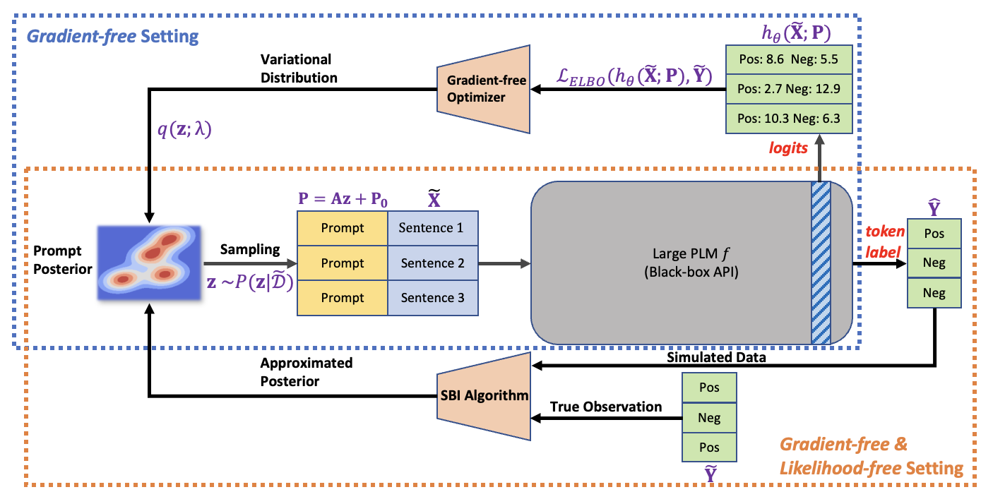
Figure 1: Our general goal is to estimate the posterior distribution of prompts. The Gradient-free setting uses the internal logits of PLM for optimization. Our proposed Gradient-free Variational inference approach utilizes the likelihood to compute the ELBO objective and leverage the gradient-free optimizer to optimize the variational distribution. The Gradient-free and likelihood-free setting can be formulated as an SBI problem, where the PLM is treated as a black-box simulator, and its output discrete outcome labels are the simulated data. The posterior samples can be efficiently approximated by the proposed ABC-SMC algorithm.

In this paper, we focus on text classification and restrict ourselves to the few-shot learning setting considered in BBT (Sun et al., 2022b). Given a dataset ${\mathcal{D}}=(\mathbf{X},\mathbf{Y})=\{({\bm{x}}_{i},y_{i})\}_{i=1}^{N}$ and a pre-trained language model (PLM) $f$, we aim to adapt $f$ to predict the label $y_{*}$ for an unseen text passage ${\bm{x}}_{*}$. We formulate the classification task as a masked language modeling problem, where the input text ${\bm{x}}_{i}$ is converted into $\tilde{{\bm{x}}}_{i}$ via predefined templates, e.g., adding trigger words like “It was [MASK]”, and the labels $y_{i}$ are mapped to label tokens $\tilde{y}_{i}$ in the vocabulary such as “great” or “bad”. We denote this transformed dataset $\tilde{{\mathcal{D}}}=(\tilde{\mathbf{X}},\tilde{\mathbf{Y}})$.

We use soft prompt tuning (Lester et al., 2021) to adapt $f$, i.e., we construct a continuous prompt embedding $\mathbf{P}\in{\mathbb{R}}^{D}$ and feed it along with the converted input text $\tilde{{\bm{x}}}_{i}$ to the PLM $f$ to generate a label token, $\hat{y}_{i}=f(\tilde{{\bm{x}}}_{i};\mathbf{P})$, where the notation $\hat{y}_{i}=f(\tilde{{\bm{x}}}_{i};\mathbf{P})$ is short hand for $\hat{y}_{i}\sim\text{Cat}(\sigma(h_{\theta}(\tilde{{\bm{x}}}_{i};\mathbf{P})))$. Here, Cat denotes the Categorical distribution, $\sigma$ is the softmax function, and $\theta$ represents the frozen parameters of the PLM. We use $h_{\theta}$ to denote all but the final layer of the PLM $f$. Finally, we aim to learn an optimal prompt

$$\mathbf{P}^{*}=\operatorname*{arg\,min}_{\mathbf{P}}-\sum_{i=1}^{N}\text{log Cat}(\tilde{y}_{i}|\sigma(h_{\theta}(\tilde{{\bm{x}}}_{i};\mathbf{P}))).$$ (1)

This is just the standard cross-entropy loss and can be easily minimized using standard stochastic gradient based approaches provided (i) we can propagate gradients through the PLM $f$, and (ii) we can access the PLM’s logits, i.e., $h_{\theta}(\tilde{{\bm{x}}}_{i};\mathbf{P})$. The problem becomes substantially more challenging when these requirements are not satisfied.

When we are unable to propagate gradients through $f$, we need to rely on gradient-free approaches to optimize Equation 1. Recent work Sun et al. (2022b) has demonstrated promising gradient-free prompt tuning results by first employing a lower dimensional re-parameterization, ${\bm{z}}\in{\mathbb{R}}^{d}$ with $d<<D$, $\mathbf{P}=\mathbf{A}{\bm{z}}+\mathbf{P_{0}}$, where $\mathbf{A}\in{\mathbb{R}}^{D\times d}$ is a random projection matrix and $\mathbf{P_{0}}$ is a fixed prompt embedding, and then using gradient-free evolutionary algorithms, in particular, Covariance Matrix Adaptation Evolution Strategy (CMA-ES) (Hansen and Ostermeier, 2001; Hansen et al., 2003) to optimize,

$${\bm{z}}^{*}$$

$$=\operatorname*{arg\,min}_{{\bm{z}}}-\sum_{i=1}^{N}\text{log Cat}(\tilde{y}_{i}|\sigma(h_{\theta}(\tilde{{\bm{x}}}_{i};\mathbf{A}{\bm{z}}+\mathbf{P_{0}}))$$ (2)

Going forward, we also adopt this lower dimensional parameterization, but instead of learning a point estimate ${\bm{z}}^{*}$, we learn a distribution $p({\bm{z}}|\tilde{{\mathcal{D}}})$ in a gradient-free setting. Similar to the point estimated variants, our algorithms to learn $p({\bm{z}}|\tilde{{\mathcal{D}}})$ also rely on CMA-ES.

Next, we consider the fully black-box setting — likelihood-free and gradient-free. Here, beyond being unable to propagate gradients through $f$, we are further handicapped by only observing the predicted label tokens, $\hat{y}_{i}=f(\tilde{{\bm{x}}}_{i};\mathbf{P})$ for each training instance $\tilde{{\bm{x}}}_{i}$, and not the corresponding logits, i.e., $h_{\theta}(\tilde{{\bm{x}}}_{i};\mathbf{P})$. In this more challenging setting we found CMA-ES based approaches to be unreliable, often getting stuck in poor optima. Instead, we found it effective to pose the likelihood-free and gradient-free prompt tuning task as a simulation-based inference (SBI) (Cranmer et al., 2020) problem. We view the PLM $f$ as a black-box simulator that given a realization of ${\bm{z}}$ and the text $\tilde{{\bm{x}}}_{i}$ produces $\hat{y}_{i}$. We then use a sequential Monte-Carlo approximate Bayesian computation (SMC-ABC) approach to infer the distribution $p({\bm{z}}|\tilde{{\mathcal{D}}})$.

Finally, we use the distribution $p({\bm{z}}|\tilde{{\mathcal{D}}})$ to characterize the uncertainty in predictions via the predictive distribution $p(\tilde{y}|\tilde{{\bm{x}}},\tilde{{\mathcal{D}}})=\int p(\tilde{y}|\tilde{{\bm{x}}};{\bm{z}})p({\bm{z}}|\tilde{{\mathcal{D}}})d{\bm{z}}$. We form Monte-Carlo approximations to this integral. In the gradient-free case, this is,

$$p(\tilde{y}|\tilde{{\bm{x}}},\tilde{{\mathcal{D}}})\approx\frac{1}{S}\sum_{s=1}^{S}p(\tilde{y}|\tilde{{\bm{x}}};{\bm{z}}_{s}),$$

where ${\bm{z}}_{s}\sim p({\bm{z}}|\tilde{{\mathcal{D}}})$. In the likelihood-free and gradient-free case, since we only have access to the label tokens, we approximate the predictive distribution,

$$p(\tilde{y}=c|\tilde{{\bm{x}}};\tilde{{\mathcal{D}}})\approx\frac{1}{S}\sum_{s=1}^{S}\mathds{1}\{\hat{y}_{s}=c\},$$ (3)

where $\hat{y}_{s}=f({\bm{x}};\mathbf{A}{\bm{z}}_{s}+\mathbf{P}_{0})$, ${\bm{z}}_{s}\sim p({\bm{z}}|\tilde{{\mathcal{D}}})$. In Section 5 we empirically demonstrate that by characterizing the uncertainty in ${\bm{z}}$ through $p({\bm{z}}|\tilde{{\mathcal{D}}})$ we get better calibrated predictive uncertainties, improved selective classification, and out-of-distribution detection.

4 Methods

We now describe our methods in greater detail. First, we discuss two algorithms for the gradient-free setting in 4.1 and 4.2. After that, we focus on addressing the gradient-free and likelihood-free setting from the SBI perspective in 4.3.

4.1 Prompt Ensembles

Deep ensembles (Lakshminarayanan et al., 2017) are a simple yet effective technique for quantifying uncertainty in deep neural network predictions. They generate a uniformly-weighted ensemble by re-training the same neural network from different random initialization. Leveraging the CMA-ES algorithm (Hansen and Ostermeier, 2001; Hansen et al., 2003), we can adapt this idea to gradient-free prompt tuning.

CMA-ES is an evolutionary strategy that maintains a multivariate normal distribution ${\mathcal{N}}(m_{t},\sigma^{2}_{t}C_{t})$ over a population of solutions. Each iteration of the algorithm involves sampling a set of possible solutions and updating the normal distribution to favor low loss solutions. To build a prompt ensemble, we run $S$ instances of CMA-ES, each initialized with a different random initialization of the mean $m_{t}$ and variance $\sigma^{2}_{t}$ and record the optimized prompt embeddings produced by each instance. This collection of $S$ prompt embeddings $\{{\bm{z}}_{s}\}_{s=1}^{S}$ form the distribution $p({\bm{z}}|\tilde{{\mathcal{D}}})$ and are used to approximate the predictive distribution via Equation 2.

4.2 Gradient-free Variational Inference

An alternative way to estimate the predictive distribution is by approximating the posterior distribution of prompt embedding $p({\bm{z}}|\tilde{{\mathcal{D}}})$. Since direct computation of posterior is intractable, in our setting we resort to variational inference (VI) and approximate the posterior distribution with a tractable surrogate $q({\bm{z}};\bm{\lambda})$, where $\bm{\lambda}$ denotes the variational parameters. VI minimizes KL-divergence between variational distribution and true posterior distribution with respect to $\bm{\lambda}$. i.e., $\bm{\lambda}^{\star}=\operatorname*{arg\,min}_{\bm{\lambda}}\mathrm{KL}\left(q({\bm{z}};\bm{\lambda})\|p({\bm{z}}|\tilde{{\mathcal{D}}})\right)$. This is equivalent to maximizing the evidence lower bound (ELBO), i.e.,

$$\bm{\lambda}^{\star}$$

$$= \operatorname*{arg\,max}_{\bm{\lambda}}\;\mathbb{E}_{q({\bm{z}};\bm{\lambda})}[\log p(\tilde{{\mathcal{D}}}|{\bm{z}})]$$ (4)

$$-\mathrm{KL}\left(q({\bm{z}};\bm{\lambda})\|p({\bm{z}})\right)$$

$$= \operatorname*{arg\,max}_{\bm{\lambda}}\;\sum_{i=1}^{N}\mathbb{E}_{q({\bm{z}};\bm{\lambda})}[\text{log Cat}(\tilde{y}_{i}|\sigma(h_{\theta}(\tilde{{\bm{x}}}_{i};\mathbf{P}))]$$

$$-\mathrm{KL}\left(q({\bm{z}};\bm{\lambda})\|p({\bm{z}})\right),$$ (5)

where $\mathbf{P}=\mathbf{A}{\bm{z}}+\mathbf{P_{0}}$, and $p({\bm{z}})$ denotes the prior distribution, which is assumed to be a normal distribution with zero mean and diagonal covariance matrix, i.e., ${\mathcal{N}}(0,\sigma\cdot\bm{I})$. Optimizing the ELBO objective requires taking derivative w.r.t $\bm{\lambda}$ as well as computing the gradient of log likelihood w.r.t ${\bm{z}}$, i.e., $\nabla_{{\bm{z}}}\mathbb{E}_{q({\bm{z}};\bm{\lambda})}[\text{log Cat}(\tilde{y}_{i}|\sigma(h_{\theta}(\tilde{{\bm{x}}}_{i};\mathbf{A}{\bm{z}}+\mathbf{P_{0}}))]$, which causes standard variational inference algorithms to be infeasible in the gradient-free setting.

Instead of back-propagation, we propose a gradient-free variational inference algorithm leveraging the derivative-free optimizer CMA-ES. Specifically, we consider the variational distribution as a multivariate normal distribution $q({\bm{z}};\bm{\lambda})={\mathcal{N}}(\bm{\mu},\bm{\Sigma})$, where we assume the covariance matrix is diagonal, i.e., $\bm{\Sigma}=\operatorname{diag}(\bm{\alpha})\in{\mathbb{R}}^{d\times d}$. The variational parameter, as the target for optimization, is the mean and diagonal elements of the covariance matrix, i.e., $\bm{\lambda}=(\bm{\mu},\bm{\alpha})\in{\mathbb{R}}^{2d}$. At each iteration of the optimization, the CMA-ES outputs a collection of candidate solutions $\{\bm{\lambda}_{j}\}_{j=1}^{m}=\{(\bm{\mu}_{j},\bm{\alpha}_{j})\}_{j=1}^{m}$. For each candidate variational parameter $\bm{\lambda}_{j}$, we evaluate the corresponding ELBO loss using the variational distribution $q({\bm{z}};\bm{\lambda}_{j})={\mathcal{N}}(\bm{\mu}_{j},\operatorname{diag}(\bm{\alpha}_{j}))$, where the expectations in Equation 5 is approximated by Monte-Carlo samples obtained from the variational distribution. Finally, the CMA-ES optimizer takes the current collection of variational parameter $\{\bm{\lambda}_{j}\}_{j=1}^{m}$ and their corresponding ELBO loss to conduct the next iteration of optimization. The schematic of the process is shown in Figure 1, and the overall algorithm is summarized as Algorithm 1 in Appendix A.

After we obtain the optimal variational parameter $\bm{\lambda}^{\star}$ that maximizes the ELBO loss, the predictive label distribution can be estimated by taking Monte Carlo samples from the optimal variational distribution, i.e., $q({\bm{z}};\bm{\lambda}^{\star})={\mathcal{N}}(\bm{\mu}^{\star},\bm{\Sigma}^{\star})$.

4.3 SBI-based Algorithm for Likelihood-free Prompt Tuning

Now, we describe our proposed approach for the gradient-free and likelihood-free case. For this problem, the most naive algorithm applicable is rejection approximation Bayesian computation (ABC) (Pritchard et al., 1999) that repeatedly samples from a prior distribution ${\bm{z}}\sim p({\bm{z}})$ and obtains the corresponding simulated observation $\hat{\mathbf{Y}}$. The algorithm only accepts the sampled prompt embedding if the simulated observation is sufficiently close to the ground truth observation $\tilde{\mathbf{Y}}$ based on a distance function $\rho$ and tolerance $\epsilon$, i.e., $\rho(\hat{\mathbf{Y}},\tilde{\mathbf{Y}})<\epsilon$. The collection of accepted samples can be used to approximate the posterior distribution. However, rejection ABC typically suffers from poor computational efficiency, especially when $\epsilon$ is small and the dimensionality of observations is large. In preliminary experiments, we found rejection ABC to not be effective for our purposes. Instead, in this work, we adapt a more advanced technique — sequential Monte Carlo approximate Bayesian computation (ABC-SMC) algorithm (McKinley et al., 2009) to enable efficient prompt posterior inference. The core idea of ABC-SMC is to use a sequential tolerance schedule, i.e., $\epsilon_{1}>\epsilon_{2}>,\ldots,>\epsilon_{T}$ to construct a sequence of intermediate distributions, which gradually converges to the true posterior distribution.

First, we draw prompt embedding samples from the prior $p({\bm{z}})={\mathcal{N}}(0,\sigma\cdot\bm{I})$ and pass them into PLM $f$ to receive the corresponding token label prediction $\hat{\mathbf{Y}}$ for a batch of text data $\tilde{\mathbf{X}}$. Then, we accept $S$ samples $\{{\bm{z}}_{s}^{(1)}\}_{s=1}^{S}$ that satisfy the condition $\rho(\hat{\mathbf{Y}},\tilde{\mathbf{Y}})<\epsilon_{1}$. We use accuracy as the distance function $\rho$. In the next iteration, we resample embeddings from $\{{\bm{z}}_{s}^{(t-1)}\}_{s=1}^{S}$ with probability proportional to weights $w^{(t-1)}$, and perturb the sampled embeddings via a perturbation kernel to obtain a new sample, i.e., ${\bm{z}}^{(t)}\sim{\mathcal{N}}({\bm{z}}^{(t-1)},\bm{\Sigma}^{(t-1)})$. Again, we propagate these sampled embeddings through the PLM $f$ and accept the newly proposed embeddings, $\{{\bm{z}}_{s}^{(t)}\}_{s=1}^{S}$, if $\rho(\hat{\mathbf{Y}},\mathbf{Y})<\epsilon_{t}$, where the tolerance $\epsilon_{t}$ is decayed by one step per iteration, i.e., $\epsilon_{t+1}=\epsilon_{t}-\frac{1}{N}$, where $N$ is the total number of training data. Finally, the weights $w^{(t)}$ and the variance of the perturbation kernel are updated after each iteration (details are elaborated in Appendix B). Empirically, we find that simply using uniform weights leads to better performance (more discussion in Section 5.3). These steps are repeated for $T$ iterations until the tolerance $\epsilon_{T}$ is sufficiently small. The schematic is in Figure 1 and the overall algorithm is summarized as Algorithm 1 in Appendix A.

The final collection of prompt samples $\{{\bm{z}}_{s}^{(T)}\}_{s=1}^{S}$ form an approximation to the posterior $p({\bm{z}}|\tilde{{\mathcal{D}}})$ and we use Equation 3 to derive the approximate predictive distribution.

5 Experiment Results

In this section, we demonstrate the solid empirical performance of our proposed methods. We begin with introducing the uncertainty quantification applications and describe the experiment settings. Then, we present our main results in terms of prediction performance and UQ quality. Finally, we provide an ablation study and relevant perspectives of comparison. Detailed results and implementation steps are provided in Appendix D.

Table 1: Prediction Performance (Test acc $\bm{\uparrow}$), *indicates results taken from BBT (Sun et al., 2022b)

Settings	Methods	SST-2	Yelp P.	AG’s News	DBPedia	MRPC	SNLI	RTE	Avg
Gradient-based	Prompt Tuning*	68.23$\pm$3.78	61.02$\pm$6.65	84.81$\pm$0.66	87.75$\pm$1.48	51.61$\pm$8.67	36.13$\pm$1.51	54.69$\pm$3.79	63.46
	P-Tuning v2*	64.33$\pm$3.05	92.63$\pm$1.39	83.46$\pm$1.01	97.05$\pm$0.41	68.14$\pm$3.89	36.89$\pm$0.79	50.78$\pm$2.28	70.47
	Model Tuning*	85.39$\pm$2.84	91.82$\pm$0.79	86.36$\pm$1.85	97.98$\pm$0.14	77.35$\pm$5.70	54.64$\pm$5.29	58.60$\pm$6.21	78.88
Gradient-free	Manual Prompt*	79.82	89.65	76.96	41.33	67.40	31.11	51.62	62.56
	In-Context Learning*	79.79$\pm$3.06	85.38$\pm$3.92	62.21$\pm$13.46	34.83$\pm$7.59	45.81$\pm$6.67	47.11$\pm$0.63	60.36$\pm$1.56	59.36
	Feature-MLP*	64.80$\pm$1.78	79.20$\pm$2.26	70.77$\pm$0.67	87.78$\pm$0.61	68.40$\pm$0.86	42.01$\pm$0.33	53.43$\pm$1.57	66.63
	Feature-BiLSTM*	65.95$\pm$0.99	74.68$\pm$0.10	77.28$\pm$2.83	90.37$\pm$3.10	71.55$\pm$7.10	46.02$\pm$0.38	52.17$\pm$0.25	68.29
	BBT	86.93$\pm$0.25	91.61$\pm$0.29	83.22$\pm$0.42	76.94$\pm$1.22	75.95$\pm$2.30	45.38$\pm$0.02	50.54$\pm$0.36	72.94
	Ours(ELBO)	86.81$\pm$0.47	92.07$\pm$0.17	83.96$\pm$0.22	73.25$\pm$2.35	76.35$\pm$0.94	46.78$\pm$2.92	50.78$\pm$1.39	72.86
	Ours(Ensembles)	88.61$\pm$0.78	92.35$\pm$0.16	84.62$\pm$0.20	80.12$\pm$1.06	76.77$\pm$1.13	47.95$\pm$2.76	50.34$\pm$3.40	74.39
Gradient-free &	Ours(SNPE)	84.37$\pm$0.29	90.38$\pm$0.07	80.50$\pm$0.10	33.11$\pm$0.48	81.02$\pm$0.06	39.60$\pm$0.49	53.07$\pm$0.82	66.01
Likelihood-free	Ours(ABC-SMC)	86.51$\pm$0.55	90.32$\pm$0.03	81.43$\pm$0.41	57.41$\pm$0.90	80.78$\pm$0.07	40.81$\pm$0.24	53.37$\pm$0.30	70.09

Table 2: Calibration Performance (ECE score $\bm{\downarrow}$)

Settings	Methods	SST-2	Yelp P.	AG’s News	DBPedia	MRPC	SNLI	RTE	Avg
Gradient-free	BBT	0.056$\pm$0.014	0.032$\pm$0.000	0.049$\pm$0.007	0.056$\pm$0.032	0.115$\pm$0.018	0.040$\pm$0.008	0.170$\pm$0.069	0.074
	Ours(ELBO)	0.056$\pm$0.007	0.025$\pm$0.004	0.065$\pm$0.001	0.045$\pm$0.028	0.058$\pm$0.004	0.035$\pm$0.007	0.113$\pm$0.030	0.057
	Ours(Ensembles)	0.058$\pm$0.001	0.017$\pm$0.001	0.064$\pm$0.009	0.085$\pm$0.005	0.073$\pm$0.007	0.039$\pm$0.004	0.134$\pm$0.033	0.067
Gradient-free &	Ours(SNPE)	0.104$\pm$0.005	0.082$\pm$0.000	0.100$\pm$0.010	0.549$\pm$0.004	0.314$\pm$0.001	0.185$\pm$0.011	0.466$\pm$0.002	0.257
Likelihood-free	Ours(ABC-SMC)	0.106$\pm$0.009	0.084$\pm$0.001	0.108$\pm$0.001	0.278$\pm$0.026	0.309$\pm$0.009	0.178$\pm$0.002	0.458$\pm$0.004	0.217

Table 3: Selective Classification (AURRRC score $\bm{\downarrow}$)

Settings	Methods	SST-2	Yelp P.	AG’s News	DBPedia	MRPC	SNLI	RTE	Avg
	Lower-bound	0.030	0.009	0.035	0.070	0.251	0.427	0.255	0.154
Gradient-free	BBT(Entropy)	0.063$\pm$0.009	0.029$\pm$0.001	0.082$\pm$0.004	0.095$\pm$0.009	0.349$\pm$0.002	0.519$\pm$0.032	0.523$\pm$0.004	0.237
	BBT(MaxP)	0.063$\pm$0.009	0.029$\pm$0.001	0.077$\pm$0.004	0.091$\pm$0.009	0.349$\pm$0.002	0.513$\pm$0.031	0.523$\pm$0.004	0.235
	ELBO(Entropy)	0.053$\pm$0.004	0.026$\pm$0.001	0.079$\pm$0.001	0.123$\pm$0.006	0.336$\pm$0.009	0.481$\pm$0.065	0.508$\pm$0.012	0.229
	ELBO(MaxP)	0.053$\pm$0.004	0.026$\pm$0.001	0.074$\pm$0.002	0.117$\pm$0.005	0.336$\pm$0.009	0.478$\pm$0.062	0.508$\pm$0.012	0.227
	Ensembles(Entropy)	0.046$\pm$0.006	0.023$\pm$0.001	0.074$\pm$0.002	0.084$\pm$0.004	0.324$\pm$0.011	0.472$\pm$0.048	0.513$\pm$0.048	0.219
	Ensembles(MaxP)	0.046$\pm$0.006	0.023$\pm$0.001	0.068$\pm$0.002	0.076$\pm$0.004	0.324$\pm$0.011	0.469$\pm$0.047	0.513$\pm$0.048	0.217
Gradient-free &	SNPE(Entropy)	0.065$\pm$0.003	0.073$\pm$0.001	0.116$\pm$0.005	0.551$\pm$0.001	0.319$\pm$0.003	0.580$\pm$0.009	0.466$\pm$0.003	0.310
Likelihood-free	SNPE(MaxP)	0.065$\pm$0.003	0.073$\pm$0.001	0.116$\pm$0.005	0.552$\pm$0.002	0.319$\pm$0.003	0.591$\pm$0.009	0.466$\pm$0.003	0.312
	ABC-SMC(Entropy)	0.061$\pm$0.006	0.075$\pm$0.002	0.110$\pm$0.004	0.285$\pm$0.015	0.325$\pm$0.006	0.571$\pm$0.000	0.468$\pm$0.014	0.271
	ABC-SMC(MaxP)	0.061$\pm$0.006	0.075$\pm$0.002	0.110$\pm$0.004	0.288$\pm$0.014	0.325$\pm$0.006	0.579$\pm$0.000	0.468$\pm$0.014	0.272

Table 4: Far OOD Detection (AURRRC score $\bm{\downarrow}$)

Settings	Methods	ID:SST-2 OOD:RTE	ID:Yelp P. OOD:RTE	ID:MRPC OOD:RTE	ID:DBPedia OOD:AG’s News	ID:SNLI OOD:MRPC	ID:RTE OOD:MRPC	Avg
	Lower-bound	0.072	0.001	0.162	0.010	0.004	0.357	0.101
Gradient-free	BBT(entropy)	0.124$\pm$0.015	0.002$\pm$0.000	0.404$\pm$0.006	0.058$\pm$0.018	0.100$\pm$0.002	0.639$\pm$0.024	0.221
	BBT(MaxP)	0.124$\pm$0.015	0.002$\pm$0.000	0.404$\pm$0.006	0.059$\pm$0.014	0.098$\pm$0.002	0.639$\pm$0.024	0.221
	Ours(ELBO)(Entropy)	0.112$\pm$0.010	0.001$\pm$0.000	0.320$\pm$0.014	0.051$\pm$0.001	0.109$\pm$0.002	0.635$\pm$0.003	0.205
	Ours(ELBO)(MaxP)	0.112$\pm$0.010	0.001$\pm$0.000	0.320$\pm$0.014	0.056$\pm$0.001	0.107$\pm$0.002	0.635$\pm$0.003	0.205
	Ours(Ensembles)(Entropy)	0.097$\pm$0.008	0.001$\pm$0.000	0.350$\pm$0.038	0.057$\pm$0.003	0.110$\pm$0.001	0.606$\pm$0.047	0.204
	Ours(Ensembles)(MaxP)	0.097$\pm$0.008	0.001$\pm$0.000	0.350$\pm$0.038	0.058$\pm$0.002	0.108$\pm$0.001	0.606$\pm$0.047	0.203
Gradient-free &	Ours(SNPE)(Entropy)	0.140$\pm$0.001	0.005$\pm$0.000	0.402$\pm$0.005	0.082$\pm$0.003	0.093$\pm$0.001	0.592$\pm$0.008	0.219
Likelihood-free	Ours(SNPE)(MaxP)	0.140$\pm$0.001	0.005$\pm$0.000	0.402$\pm$0.005	0.081$\pm$0.003	0.091$\pm$0.002	0.592$\pm$0.008	0.219
	Ours(ABC-SMC)(Entropy)	0.126$\pm$0.009	0.005$\pm$0.001	0.396$\pm$0.001	0.097$\pm$0.021	0.092$\pm$0.000	0.596$\pm$0.009	0.219
	Ours(ABC-SMC)(MaxP)	0.126$\pm$0.009	0.005$\pm$0.001	0.396$\pm$0.001	0.095$\pm$0.021	0.092$\pm$0.001	0.596$\pm$0.009	0.218

Table 5: Near OOD Detection (AURRRC score $\bm{\downarrow}$)

Settings	Methods	ID:SST-2 OOD:IMDB	ID:Yelp P. OOD:IMDB	ID:SNLI OOD:MNLI	ID:RTE OOD:MNLI	Avg
	Lower-bound	0.960	0.147	0.259	0.950	0.579
Gradient-free	BBT(entropy)	0.978$\pm$0.003	0.315$\pm$0.003	0.720$\pm$0.011	0.963$\pm$0.008	0.744
	BBT(confidence)	0.978$\pm$0.003	0.315$\pm$0.003	0.705$\pm$0.011	0.963$\pm$0.008	0.740
	Ours(ELBO)(Entropy)	0.976$\pm$0.002	0.308$\pm$0.006	0.692$\pm$0.039	0.968$\pm$0.005	0.736
	Ours(ELBO)(MaxP)	0.976$\pm$0.002	0.308$\pm$0.006	0.678$\pm$0.044	0.968$\pm$0.005	0.733
	Ours(Ensembles)(Entropy)	0.976$\pm$0.001	0.297$\pm$0.003	0.707$\pm$0.028	0.962$\pm$0.002	0.736
	Ours(Ensembles)(MaxP)	0.976$\pm$0.001	0.297$\pm$0.003	0.692$\pm$0.032	0.962$\pm$0.002	0.732
Gradient-free &	Ours(SNPE)(Entropy)	0.984$\pm$0.000	0.365$\pm$0.001	0.715$\pm$0.002	0.951$\pm$0.000	0.754
Likelihood-free	Ours(SNPE)(MaxP)	0.984$\pm$0.000	0.365$\pm$0.001	0.695$\pm$0.004	0.951$\pm$0.000	0.749
	Ours(ABC-SMC)(Entropy)	0.983$\pm$0.001	0.365$\pm$0.001	0.710$\pm$0.002	0.952$\pm$0.000	0.753
	Ours(ABC-SMC)(MaxP)	0.983$\pm$0.001	0.365$\pm$0.001	0.694$\pm$0.000	0.952$\pm$0.000	0.749

5.1 Settings

Uncertainty Quantification Applications.

We assess the performance of the uncertainty quantification from three perspectives: (1) Calibration – the typical UQ quality metric that measures how well the model confidence aligned with the correctness of its prediction; (2) Selective Classification – aims to avoid the risk of wrong predictions by abstaining the prediction for samples with high uncertainty; and (3) OOD Detection – aims to identify the out-of-distribution data that is unobserved during the training stage. The OOD data can exhibit different forms of distribution shift, including the covariate shift where the OOD data distribution is different from the training samples; and the semantic shift where the OOD data contain unobserved class. In our experiment, we focus on two types of OOD tasks: the Far OOD detection task where both covariat shift and semantic shift happen simultaneously; the Near OOD detection task where the OOD data only contain covariate shift, but have the same class label words.

Benchmark.

For a comprehensive comparison with BBT (Sun et al., 2022b), we mainly employ the same text classification benchmark datasets as BBT, including sentiment analysis datasets SST-2 (Socher et al., 2013) and Yelp polarity (Zhang et al., 2015); topic classification datasets AG’s News (Zhang et al., 2015) and DBPedia (Zhang et al., 2015); paraphrase dataset MRPC (Dolan and Brockett, 2005); natural language inference (NLI) datasets SNLI (Bowman et al., 2015) and RTE (Wang et al., 2018).

Both calibration and selective classification tasks are conducted using the original test samples for each benchmark dataset. For the far OOD detection task, we create the ID/OOD dataset pairs by combining two datasets belonging to two different tasks, e.g., SST-2/RTE. For the near OOD detection task, we use IMDB (Maas et al., 2011) for the sentiment analysis task and MNLI (Williams et al., 2017) for the NLI task.

Baselines.

For prediction performance, besides the SOTA Gradient-free prompt tuning approach BBT (Sun et al., 2022b), we also compare with other Gradient-free methods: (1) The naive Manual Prompt that uses the hand-crafted prompt templates; (2) In-context Learning (Brown et al., 2020); (3) Feature-based approaches (Peters et al., 2019) that trains auxiliary models on top of the PLM extracted features, including Feature-MLP training a MLP classifier and Feature-BiLSTM training a LSTM model followed by a classifier. We include additional results of Gradient-based approaches: (1) Model Tuning that fine-tunes the entire PLM; (2) Prompt Tuning (Lester et al., 2021) that only trains the continuous prompt without modifying PLM; (3) P-Tuning v2 (Liu et al., 2021b) that trains the several continuous prompts injected at different layers of PLM. For uncertainty quantification tasks, few existing prompt tuning works aim to tackle this problem, so we mainly compare with BBT to justify how we can address its limitation under the gradient-free setting.

Implementation Details.

We follow the same experiment setting as BBT. We focus on text classification as a few-shot learning problem, motivated by the fact that labeled training data can be limited in practice. Specifically, we construct few-shot training and validation data by drawing $16$ random samples for each class from the original training dataset. The prediction performance is evaluated on the original development or test set, depending on the datasets. We use the same PLM model $\operatorname{RoBERTa_{LARGE}}$ as the backbone model and keep the hyper-parameter same as BBT. Specifically, we set the prompt length as $50$, i.e., $D=50\times 1024$, and the subspace dimensionality as $d=500$. The only modification is that we adapt the normal distribution (Sun et al., 2022a) to generate the random projection matrix $\mathbf{A}$, instead of the uniform distribution used in BBT. For a fair comparison, we reproduce the results of BBT using the random projection generated from normal distribution. More implementation details are included in Appendix C.

Performance Metrics.

For prediction performance, we evaluate the prediction accuracy on the testing dataset. For calibration performance, we adopt the expected calibration error (ECE) (Guo et al., 2017) score as the metric. For both selective classification and OOD detection tasks, we compute the area under the risk vs. rejection rate curve (AURRRC) (Franc and Prusa, 2019). The risk is defined as the portion of wrong-predicted samples among the data chosen for prediction in selective classification and the portion of OOD samples among the data identified as in-distribution in the OOD detection task. The rejection rate is defined as the portion of data that abstained from the prediction based on specific uncertainty measurement. Note that an oracle with perfect knowledge of uncertainty measurement can achieve a minimum AURRRC score. This is obtained by assigning an uncertainty score based on the oracle knowledge, i.e., whether a test sample is wrong-predicted (OOD samples) or not. We denote such minimum AURRRC score as the lower-bound.

Given the predictive label distribution, we utilize two uncertainty measurements, including Entropy of the label distribution, i.e., ${\mathcal{H}}\left(p(\tilde{y}|\tilde{{\bm{x}}};\tilde{{\mathcal{D}}})\right)$, and MaxP, which is defined as $\max_{c}p(\tilde{y}=c|\tilde{{\bm{x}}};\tilde{{\mathcal{D}}})$.

5.2 Results

We conduct extensive evaluations of our proposed methods under both the Gradient-free setting and the Gradient-free and Likelihood-free setting. The results of prediction performance are shown in Table 1. For the uncertainty quantification performance, the calibration results are shown in Table 2, the selective classification results are shown in Table 3, the Far OOD detection results are shown in Table 4 and the Near OOD detection results are shown in Table 5.

Gradient-free and Likelihood-free Setting.

No existing work is trying to tackle the Gradient-free and likelihood-free prompt tuning problem. However, we still compare our proposed method with other baseline methods on different problem settings to understand how well we can achieve and the price we need to pay for such a more strict constraint. In addition, we also include the results of neural net-based approach SNPE (Hermans et al., 2020; Durkan et al., 2020) for solving the SBI problem.

As shown in Table 1, our proposed method ABC-SMC can achieve competitive prediction performance as SOTA approach BBT and even outperform the other Gradient-free baselines without the requirement of the model likelihood. We also observe that ABC-SMC performs better than SNPE. The possible explanation is that the density estimation model adopted by SNPE usually requires a large number of simulated samples to achieve good performance, which is hindered by the slow inference speed of large PLM.

For the uncertainty quantification tasks, ABC-SMC underperforms on calibration and selective classification tasks but can still achieve comparable performance on the two OOD detection tasks. The performance gap can possibly be mitigated if we collect more samples (by increasing $K$) for a more accurate estimation of the empirical label distribution, but the computational cost is the price we need to pay for the likelihood-free constraint.

Gradient-free Setting.

By relaxing the likelihood-free constraint, it is observed that our proposed methods, both Gradient-free Variational Inference (denoted as ELBO) and Ensembles algorithms, achieve comparable or even better prediction performance than BBT and other gradient-free baselines, while outperforming BBT in terms of uncertainty quantification across all the tasks. Such empirical observation justifies the effectiveness of leveraging Bayesian and Ensemble techniques to enable more reliable gradient-free prompt tuning without sacrificing the prediction performance.

5.3 Discussions

In this section, we further investigate our proposed methods by exploring the use of alternate models and the effect of using uniform weights in the SMC-ABC algorithm.

Performance on other backbone models

To demonstrate that our proposed methods generalize well on other PLM backbone models, we evaluate them on $\operatorname{BERT_{LARGE}}$ under the both Gradient-free setting and Gradient-free and likelihood-free setting. The results are presented in Appendix D.1. Note that our proposed methods consistently outperform BBT in terms of both prediction and uncertainty quantification performance under the Gradient-free setting while achieving competitive performance with a small gap under the Gradient-free and likelihood-free setting.

Ablation study of weights in ABC-SMC

In practice, we observe that the ABC-SMC algorithm suffers from weight degeneracy, with weights for certain particles approaching one and effectively causing the posterior to be approximated by a single particle. Although, this issue can be mitigated by designing better proposals, we found that the heuristic of using uniform weights instead of updating the weights at each iteration of the algorithm to be far more effective. To demonstrate the efficacy, we conduct an ablation study about the sampling weights, and the results are shown in Appendix D.2. We find that with uniform weights ABC-SMC provides both improves prediction and uncertainty quantification for our application.

6 Concluding Remarks

In this work, we explore gradient-free prompt tuning along two under-explored angles: quantifying uncertainty in soft prompts; and tackling a more strict likelihood-free setting from the SBI perspective. Our developed methods demonstrate encouraging empirical performance across multiple tasks.

Investigating more modern neural SBI methods and designing more robust methods for learning prompt posteriors are exciting directions for future research. Other perspectives on gradient-free prompt tuning, such as learning natural language-like interpretable prompts, are also worthy of exploration.

7 Limitations

We explored methods for learning a distribution over prompts for tuning PLMs with only API access. We rely on approximate inference algorithms to infer these distributions. Since the true posterior is intractable, effectively evaluating the quality of the inferred approximate posteriors is challenging. Here, we use downstream metrics to compare different algorithms. However, such metrics conflate the quality of posterior approximation with predictive performance. Assessing the quality of approximate posteriors remains an open problem. Another limitation of our ABC-based approach is that it is more expensive than approaches that can exploit gradient information. Improving the computational efficiency of such approaches comprises interesting future work.

8 Acknowledgements

This work was supported, in part, by the MIT-IBM Watson AI Lab under Agreement No. W1771646, and NSF under Grant No. CCF-1816209.

Appendix A Omitted Algorithms

The overall algorithm of Gradient-free Variational Inference and ABC-SMC are shown in Algorithm 1 and Algorithm 2, respectively.

input Training data set $\{(\tilde{{\bm{x}}}_{i},\tilde{y}_{i})\}_{i=1}^{N}$; CMA-ES optimizer $\operatorname{ES}$; Prior distribution $p({\bm{z}})$; Number of candidate solutions $m$; Total iteration $T$.

Initialize the initial collection of variational parameter, i.e., $\{\bm{\lambda}^{(0)}_{j}\}_{j=1}^{m}=\{(\bm{\mu}^{(0)}_{j},\bm{\alpha}^{(0)}_{j})\}_{j=1}^{m}$.
for $t=1,2,\ldots,T$ do

       for $j=1,2,\ldots,m$ do

             Generate $S$ prompt embedding samples from the variational distribution, i.e.,

$$\{{\bm{z}}^{(t-1)}_{s}\}_{s=1}^{S}\sim{\mathcal{N}}\left(\bm{\mu}_{j}^{(t-1)},\operatorname{diag}(\bm{\alpha}_{j}^{(t-1)})\right)$$

Evaluate the ELBO loss of $j$-th variational distribution i.e.,

$${\mathcal{L}}_{j}^{(t-1)}$$

$$=\sum_{i=1}^{N}\sum_{s=1}^{S}\text{log Cat}(\tilde{y}_{i}|\sigma(h_{\theta}(\tilde{{\bm{x}}}_{i};\mathbf{A}{\bm{z}}^{(t-1)}_{s}+\mathbf{P_{0}}))$$

$$-\mathrm{KL}\left(q({\bm{z}};\bm{\lambda}_{j}^{(t-1)})\|p({\bm{z}})\right)$$

       end for

      Request a new collection of variational parameter solutions, i.e.,

$$\{\bm{\lambda}^{(t)}_{j}\}_{j=1}^{m}\leftarrow\operatorname{ES}\left(\{\bm{\lambda}^{(t-1)}_{j}\}_{j=1}^{m};\{{\mathcal{L}}_{j}^{(t-1)}\}_{j=1}^{m}\right)$$

end for

output Optimized collection of prompt embedding samples $\{{\bm{z}}^{(T)}_{s}\}_{s=1}^{S}$ corresponding to max ELBO loss.

Algorithm 1 Gradient-free Variational Inference

input PLM $f$; The fixed random projection matrix $\mathbf{A}$ and intial prompt $\mathbf{P_{0}}$; Training data set $(\tilde{\mathbf{X}},\tilde{\mathbf{Y}})=\{(\tilde{{\bm{x}}}_{i},\tilde{y}_{i})\}_{i=1}^{N}$; Prior distribution $p({\bm{z}})$; Initial tolerance $\epsilon_{1}$; Distance measure function $\rho(\cdot)$; Number of samples $S$; Total iteration $T$.

for $t=1,2,\ldots,T$ do

       if $t==1$ then

             for $s=1,2,\ldots,S$ do

                   do

                         Generate prompt embedding samples from the prior distribution, i.e., ${\bm{z}}_{s}^{(1)}\sim p({\bm{z}})$; Obtain the corresponding prediction result $\hat{\mathbf{Y}}=f(\mathbf{A}{\bm{z}}_{s}^{(1)}+\mathbf{P_{0}};\tilde{\mathbf{X}})$.

                  while $\rho(\hat{\mathbf{Y}},\tilde{\mathbf{Y}})>\epsilon_{1}$;

                  Initialize the sampling probability weights $w_{s}^{(1)}=\frac{1}{S}$.

             end for

            Decay the tolerance, i.e., $\epsilon_{t+1}=\epsilon_{t}-\frac{1}{N}$; Initialize the perturbation kernel variance $\bm{\Sigma}^{(1)}$.

      else

             for $s=1,2,\ldots,S$ do

                   do

                         Draw a random sample ${\bm{z}}_{s}^{(t-1)}$ from $\{{\bm{z}}^{(t-1)}_{s}\}_{s=1}^{S}$ with probability $w_{s}^{(t-1)}$; Generate a new sample ${\bm{z}}_{s}^{(t)}\sim{\mathcal{N}}({\bm{z}}_{s}^{(t-1)},\bm{\Sigma}^{(t-1)})$; Obtain the corresponding prediction result $\hat{\mathbf{Y}}=f(\mathbf{A}{\bm{z}}_{s}^{(t)}+\mathbf{P_{0}};\tilde{X})$.

                  while $\rho(\hat{\mathbf{Y}},\tilde{\mathbf{Y}})>\epsilon_{t}$;

                  Update the sampling probability weights $w^{(t)}$ (see Appendix B).

             end for

            Decay the tolerance, i.e., $\epsilon_{t+1}=\epsilon_{t}-\frac{1}{N}$; Update the perturbation kernel variance $\bm{\Sigma}^{(t)}$ (see Appendix B).

       end if

      

end for

output Optimized collection of prompt embedding samples $\{{\bm{z}}^{(T)}_{s}\}_{s=1}^{S}$; Final sampling weights $w^{(T)}$.

Algorithm 2 ABC-SMC

Appendix B Implementation details of ABC-SMC

Updating of $w^{(t)}$

In the ABC-SMC algorithm, the sampling weights are initialized as uniform distribution at the first iteration $t=1$ as all the samples are sampled from the prior distribution $p({\bm{z}})$. In the later iterations, the new samples are drawing from a mixture proposal distribution consisted the previous samples and the perturbation kernel, i.e., $\sum_{s=1}^{S}w_{s}^{(t-1)}\cdot{\mathcal{N}}({\bm{z}}_{s}^{(t-1)},\bm{\Sigma}^{(t-1)})$. The weights are updated in an importance sampling manner as the ratio between the prior probability and the proposal probability, i.e.,

$$w_{s}^{(t)}=\frac{p({\bm{z}}_{s})}{\sum_{s=1}^{S}w_{s}^{(t-1)}\cdot{\mathcal{N}}({\bm{z}}_{s}^{(t-1)},\bm{\Sigma}^{(t-1)})}$$

Updating of $\bm{\Sigma}^{(t)}$

The covariance $\bm{\Sigma}^{(t)}$ in the perturbation kernel is a diagonal covariance matrix $\operatorname{diag}(\bm{\alpha}^{(t)})$, where the diagonal elements $\bm{\alpha}^{(t)}$ are updated using the weighted empirical variance of previous collection of samples, i.e.

$$\bm{\alpha}^{(t)}=\sum_{s=1}^{S}w_{s}^{(t-1)}\cdot({\bm{z}}_{s}^{(t-1)}-\bar{{\bm{z}}}^{(t-1)})^{2}$$

Where $\bar{{\bm{z}}}^{(t-1)}=\sum_{s=1}^{S}w_{s}^{(t-1)}\cdot{\bm{z}}_{s}^{(t-1)}$ is the mean.

Appendix C Implementation Details

All of our experiment results are reported with means and standard deviations over three trials, each with a different random seed. The experiments are implemented in PyTorch, and each run of our proposed methods requires less than 24h of training computation time (on a single NVIDIA Tesla V100 GPU). Our proposed algorithms generate a collection of $S$ prompt samples to estimate the predictive label distribution. We set $S=10,100,100$ for Ensembles, Gradient-free Variational Inference, and ABC-SMC, respectively. The total budget for the derivative-free optimizer CMA-ES is set to be 300 with a population size of 20. We use the same prior distribution $p({\bm{z}})$ for all algorithms, which is assumed to be a normal distribution with zero mean and diagonal covariance matrix, i.e., ${\mathcal{N}}(0,\sigma\cdot\bm{I})$. $\sigma$ controls how concentrated the prior distribution is, and we use $\sigma=50$ in our experiments. In ABC-SMC, the distance measure function $\rho$ is defined as the prediction error rate, i.e., the portion of wrongly predicted data among the whole data batch. The initial tolerance $\epsilon_{1}$ in ABC-SMC is initialized as the prediction error rate of an arbitrary prompt sample drawing from the prior distribution. The tolerance is decayed by one step per iteration, i.e., $\epsilon_{t+1}=\epsilon_{t}-\frac{1}{N}$, where $N$ is the total number of training data.

Appendix D Additional Experiment Results

D.1 Performance on other backbone PLM

We evaluate the performance of our proposed methods on SST-2 and SNLI tasks using $\operatorname{BERT_{LARGE}}$ as the backbone model. We keep the hyper-parameter settings the same as the original experiments. The results are shown in Table 6, 7, 8, and 9.

Table 6: Test Performance (test acc $\uparrow$)

Settings	Methods	SST-2	SNLI
Gradient-free	BBT	74.77$\pm$3.21	41.07$\pm$2.97
	Ours(ELBO)	75.38$\pm$1.74	41.20$\pm$0.39
	Ours(Ensembles)	80.05$\pm$1.79	42.64$\pm$1.96
Gradient-free & Likelihood-free	Ours(ABC-SMC)	66.40$\pm$0.46	39.00$\pm$0.22

Table 7: Calibration Performance (ECE score $\bm{\downarrow}$)

Settings	Methods	SST-2	SNLI
Gradient-free	BBT	0.081$\pm$0.051	0.086$\pm$0.039
	Ours(ELBO)	0.046$\pm$0.006	0.073$\pm$0.009
	Ours(Ensembles)	0.045$\pm$0.007	0.068$\pm$0.024
Gradient-free & Likelihood-free	Ours(ABC-SMC)	0.328$\pm$0.003	0.584$\pm$0.002

Table 8: Selective Classification (AURRRC score $\bm{\downarrow}$)

Settings	Methods	SST-2	SNLI
Gradient-free	BBT(Entropy)	0.146$\pm$0.028	0.564$\pm$0.036
	BBT(MaxP)	0.146$\pm$0.028	0.568$\pm$0.043
	Ours(ELBO)(Entropy)	0.132$\pm$0.009	0.542$\pm$0.006
	Ours(ELBO)(MaxP)	0.132$\pm$0.009	0.540$\pm$0.009
	Ours(Ensembles)(Entropy)	0.104$\pm$0.014	0.525$\pm$0.023
	Ours(Ensembles)(MaxP)	0.104$\pm$0.014	0.523$\pm$0.024
Gradient-free &	Ours(ABC-SMC)(Entropy)	0.327$\pm$0.002	0.607$\pm$0.001
Likelihood-free	Ours(ABC-SMC)(MaxP)	0.327$\pm$0.002	0.607$\pm$0.001

Table 9: Far OOD Detection (AURRRC score $\bm{\downarrow}$)

Settings	Methods	ID:SST-2 OOD:RTE	ID:SNLI OOD:MRPC
Gradient-free	BBT(entropy)	0.402$\pm$0.015	0.076$\pm$0.016
	BBT(MaxP)	0.402$\pm$0.015	0.072$\pm$0.015
	Ours(ELBO)(Entropy)	0.365$\pm$0.037	0.089$\pm$0.007
	Ours(ELBO)(MaxP)	0.365$\pm$0.037	0.084$\pm$0.006
	Ours(Ensembles)(Entropy)	0.338$\pm$0.027	0.074$\pm$0.020
	Ours(Ensembles)(MaxP)	0.338$\pm$0.027	0.071$\pm$0.018
Gradient-free &	Ours(ABC-SMC)(Entropy)	0.252$\pm$0.000	0.044$\pm$0.000
Likelihood-free	Ours(ABC-SMC)(MaxP)	0.252$\pm$0.000	0.044$\pm$0.000

D.2 Ablation of ABC-SMC sampling weights

We compare both the prediction and uncertainty quantification performance of our proposed ABC-SMC approaches using the updated sampling weights and the fixed uniform weights. We denote the method using updated weights as “ABC-SMC w. Weights". The results are shown in Table 10, 11, 12, 13, and 14.

Table 10: Prediction Performance (Test acc $\bm{\uparrow}$)

Methods	SST-2	Yelp P.	AG’s News	DBPedia	MRPC	SNLI	RTE	Avg
ABC-SMC	86.51$\pm$0.55	90.32$\pm$0.03	81.43$\pm$0.41	57.41$\pm$0.90	80.78$\pm$0.07	40.81$\pm$0.24	53.37$\pm$0.30	70.09
ABC-SMC w. Weights	84.37$\pm$0.81	90.42$\pm$0.22	79.44$\pm$0.46	50.36$\pm$0.89	80.83$\pm$0.08	42.06$\pm$1.15	53.07$\pm$0.01	68.65

Table 11: Calibration Performance (ECE score $\bm{\downarrow}$)

Methods	SST-2	Yelp P.	AG’s News	DBPedia	MRPC	SNLI	RTE	Avg
ABC-SMC	0.106$\pm$0.009	0.084$\pm$0.001	0.108$\pm$0.001	0.278$\pm$0.026	0.309$\pm$0.009	0.178$\pm$0.002	0.458$\pm$0.004	0.217
ABC-SMC w. Weights	0.156$\pm$0.008	0.091$\pm$0.005	0.160$\pm$0.023	0.506$\pm$0.009	0.316$\pm$0.002	0.182$\pm$0.005	0.463$\pm$0.003	0.268

Table 12: Selective Classification (AURRRC score $\bm{\downarrow}$)

Methods	SST-2	Yelp P.	AG’s News	DBPedia	MRPC	SNLI	RTE	Avg
ABC-SMC (Entropy)	0.061$\pm$0.006	0.075$\pm$0.002	0.110$\pm$0.004	0.285$\pm$0.015	0.325$\pm$0.006	0.571$\pm$0.000	0.468$\pm$0.014	0.271
ABC-SMC(MaxP)	0.061$\pm$0.006	0.075$\pm$0.002	0.110$\pm$0.004	0.288$\pm$0.014	0.325$\pm$0.006	0.579$\pm$0.000	0.468$\pm$0.014	0.272
ABC-SMC w. Weights (Entropy)	0.090$\pm$0.008	0.069$\pm$0.002	0.125$\pm$0.002	0.442$\pm$0.011	0.315$\pm$0.001	0.570$\pm$0.019	0.460$\pm$0.006	0.296
ABC-SMC w. Weights (MaxP)	0.090$\pm$0.008	0.073$\pm$0.003	0.133$\pm$0.008	0.479$\pm$0.020	0.315$\pm$0.001	0.570$\pm$0.017	0.460$\pm$0.006	0.303

Table 13: Far OOD Detection (AURRRC score $\bm{\downarrow}$)

Methods	ID:SST-2 OOD:RTE	ID:Yelp P. OOD:RTE	ID:MRPC OOD:RTE	ID:DBPedia OOD:AG’s News	ID:SNLI OOD:MRPC	ID:RTE OOD:MRPC	Avg
ABC-SMC(Entropy)	0.126$\pm$0.009	0.005$\pm$0.001	0.396$\pm$0.001	0.097$\pm$0.021	0.092$\pm$0.000	0.596$\pm$0.009	0.219
ABC-SMC(MaxP)	0.126$\pm$0.009	0.005$\pm$0.001	0.396$\pm$0.001	0.095$\pm$0.021	0.092$\pm$0.001	0.596$\pm$0.009	0.218
ABC-SMC w. Weights(Entropy)	0.186$\pm$0.020	0.004$\pm$0.001	0.406$\pm$0.013	0.079$\pm$0.013	0.067$\pm$0.004	0.596$\pm$0.006	0.223
ABC-SMC w. Weights(MaxP)	0.186$\pm$0.020	0.004$\pm$0.001	0.402$\pm$0.006	0.091$\pm$0.002	0.057$\pm$0.004	0.596$\pm$0.006	0.223

Table 14: Near OOD Detection (AURRRC score $\bm{\downarrow}$)

Methods	ID:SST-2 OOD:IMDB	ID:Yelp P. OOD:IMDB	ID:SNLI OOD:MNLI	ID:RTE OOD:MNLI	Avg
ABC-SMC(Entropy)	0.983$\pm$0.001	0.365$\pm$0.001	0.710$\pm$0.002	0.952$\pm$0.000	0.753
ABC-SMC(MaxP)	0.983$\pm$0.001	0.365$\pm$0.001	0.694$\pm$0.000	0.952$\pm$0.000	0.749
ABC-SMC w. Weights(Entropy)	0.967$\pm$0.002	0.365$\pm$0.001	0.572$\pm$0.049	0.952$\pm$0.001	0.714
ABC-SMC W. Weights(MaxP)	0.967$\pm$0.002	0.365$\pm$0.001	0.534$\pm$0.032	0.952$\pm$0.001	0.705

References

- Arora et al. (2021) Udit Arora, William Huang, and He He. 2021. Types of out-of-distribution texts and how to detect them. arXiv preprint arXiv:2109.06827.
- Bahdanau et al. (2014) Dzmitry Bahdanau, Kyunghyun Cho, and Yoshua Bengio. 2014. Neural machine translation by jointly learning to align and translate. arXiv preprint arXiv:1409.0473.
- Beaumont et al. (2009) Mark A Beaumont, Jean-Marie Cornuet, Jean-Michel Marin, and Christian P Robert. 2009. Adaptive approximate bayesian computation. Biometrika, 96(4):983–990.
- Beaumont et al. (2002) Mark A Beaumont, Wenyang Zhang, and David J Balding. 2002. Approximate bayesian computation in population genetics. Genetics, 162(4):2025–2035.
- Bonassi and West (2015) Fernando V Bonassi and Mike West. 2015. Sequential monte carlo with adaptive weights for approximate bayesian computation. Bayesian Analysis, 10(1):171–187.
- Bowman et al. (2015) Samuel R Bowman, Gabor Angeli, Christopher Potts, and Christopher D Manning. 2015. A large annotated corpus for learning natural language inference. arXiv preprint arXiv:1508.05326.
- Brown et al. (2020) Tom Brown, Benjamin Mann, Nick Ryder, Melanie Subbiah, Jared D Kaplan, Prafulla Dhariwal, Arvind Neelakantan, Pranav Shyam, Girish Sastry, Amanda Askell, et al. 2020. Language models are few-shot learners. Advances in neural information processing systems, 33:1877–1901.
- Cranmer et al. (2020) Kyle Cranmer, Johann Brehmer, and Gilles Louppe. 2020. The frontier of simulation-based inference. Proceedings of the National Academy of Sciences, 117(48):30055–30062.
- Desai and Durrett (2020) Shrey Desai and Greg Durrett. 2020. Calibration of pre-trained transformers. arXiv preprint arXiv:2003.07892.
- Devlin et al. (2018) Jacob Devlin, Ming-Wei Chang, Kenton Lee, and Kristina Toutanova. 2018. Bert: Pre-training of deep bidirectional transformers for language understanding. arXiv preprint arXiv:1810.04805.
- Dolan and Brockett (2005) Bill Dolan and Chris Brockett. 2005. Automatically constructing a corpus of sentential paraphrases. In Third International Workshop on Paraphrasing (IWP2005).
- Durkan et al. (2020) Conor Durkan, Iain Murray, and George Papamakarios. 2020. On contrastive learning for likelihood-free inference. In International Conference on Machine Learning, pages 2771–2781. PMLR.
- Franc and Prusa (2019) Vojtech Franc and Daniel Prusa. 2019. On discriminative learning of prediction uncertainty. In International Conference on Machine Learning, pages 1963–1971. PMLR.
- Gao et al. (2020) Tianyu Gao, Adam Fisch, and Danqi Chen. 2020. Making pre-trained language models better few-shot learners. arXiv preprint arXiv:2012.15723.
- Greenberg et al. (2019) David Greenberg, Marcel Nonnenmacher, and Jakob Macke. 2019. Automatic posterior transformation for likelihood-free inference. In International Conference on Machine Learning, pages 2404–2414. PMLR.
- Guo et al. (2017) Chuan Guo, Geoff Pleiss, Yu Sun, and Kilian Q Weinberger. 2017. On calibration of modern neural networks. In International conference on machine learning, pages 1321–1330. PMLR.
- Hansen et al. (2003) Nikolaus Hansen, Sibylle D Müller, and Petros Koumoutsakos. 2003. Reducing the time complexity of the derandomized evolution strategy with covariance matrix adaptation (cma-es). Evolutionary computation, 11(1):1–18.
- Hansen and Ostermeier (2001) Nikolaus Hansen and Andreas Ostermeier. 2001. Completely derandomized self-adaptation in evolution strategies. Evolutionary computation, 9(2):159–195.
- Hermans et al. (2020) Joeri Hermans, Volodimir Begy, and Gilles Louppe. 2020. Likelihood-free mcmc with amortized approximate ratio estimators. In International Conference on Machine Learning, pages 4239–4248. PMLR.
- Kowsari et al. (2019) Kamran Kowsari, Kiana Jafari Meimandi, Mojtaba Heidarysafa, Sanjana Mendu, Laura Barnes, and Donald Brown. 2019. Text classification algorithms: A survey. Information, 10(4):150.
- Kumar and Sarawagi (2019) Aviral Kumar and Sunita Sarawagi. 2019. Calibration of encoder decoder models for neural machine translation. arXiv preprint arXiv:1903.00802.
- Lakshminarayanan et al. (2017) Balaji Lakshminarayanan, Alexander Pritzel, and Charles Blundell. 2017. Simple and scalable predictive uncertainty estimation using deep ensembles. Advances in neural information processing systems, 30.
- Lester et al. (2021) Brian Lester, Rami Al-Rfou, and Noah Constant. 2021. The power of scale for parameter-efficient prompt tuning. arXiv preprint arXiv:2104.08691.
- Lewis et al. (2019) Mike Lewis, Yinhan Liu, Naman Goyal, Marjan Ghazvininejad, Abdelrahman Mohamed, Omer Levy, Ves Stoyanov, and Luke Zettlemoyer. 2019. Bart: Denoising sequence-to-sequence pre-training for natural language generation, translation, and comprehension. arXiv preprint arXiv:1910.13461.
- Li and Liang (2021) Xiang Lisa Li and Percy Liang. 2021. Prefix-tuning: Optimizing continuous prompts for generation. arXiv preprint arXiv:2101.00190.
- Liu et al. (2021a) Pengfei Liu, Weizhe Yuan, Jinlan Fu, Zhengbao Jiang, Hiroaki Hayashi, and Graham Neubig. 2021a. Pre-train, prompt, and predict: A systematic survey of prompting methods in natural language processing. arXiv preprint arXiv:2107.13586.
- Liu et al. (2021b) Xiao Liu, Kaixuan Ji, Yicheng Fu, Zhengxiao Du, Zhilin Yang, and Jie Tang. 2021b. P-tuning v2: Prompt tuning can be comparable to fine-tuning universally across scales and tasks. arXiv preprint arXiv:2110.07602.
- Liu et al. (2021c) Xiao Liu, Yanan Zheng, Zhengxiao Du, Ming Ding, Yujie Qian, Zhilin Yang, and Jie Tang. 2021c. Gpt understands, too. arXiv preprint arXiv:2103.10385.
- Lueckmann et al. (2017) Jan-Matthis Lueckmann, Pedro J Goncalves, Giacomo Bassetto, Kaan Öcal, Marcel Nonnenmacher, and Jakob H Macke. 2017. Flexible statistical inference for mechanistic models of neural dynamics. Advances in neural information processing systems, 30.
- Maas et al. (2011) Andrew Maas, Raymond E Daly, Peter T Pham, Dan Huang, Andrew Y Ng, and Christopher Potts. 2011. Learning word vectors for sentiment analysis. In Proceedings of the 49th annual meeting of the association for computational linguistics: Human language technologies, pages 142–150.
- Marin et al. (2012) Jean-Michel Marin, Pierre Pudlo, Christian P Robert, and Robin J Ryder. 2012. Approximate bayesian computational methods. Statistics and Computing, 22(6):1167–1180.
- Marjoram et al. (2003) Paul Marjoram, John Molitor, Vincent Plagnol, and Simon Tavaré. 2003. Markov chain monte carlo without likelihoods. Proceedings of the National Academy of Sciences, 100(26):15324–15328.
- McKinley et al. (2009) Trevelyan McKinley, Alex R Cook, and Robert Deardon. 2009. Inference in epidemic models without likelihoods. The International Journal of Biostatistics, 5(1).
- Papamakarios et al. (2019) George Papamakarios, David Sterratt, and Iain Murray. 2019. Sequential neural likelihood: Fast likelihood-free inference with autoregressive flows. In The 22nd International Conference on Artificial Intelligence and Statistics, pages 837–848. PMLR.
- Peters et al. (2018) Matthew E. Peters, Mark Neumann, Mohit Iyyer, Matt Gardner, Christopher Clark, Kenton Lee, and Luke Zettlemoyer. 2018. Deep contextualized word representations. In NAACL.
- Peters et al. (2019) Matthew E Peters, Sebastian Ruder, and Noah A Smith. 2019. To tune or not to tune? adapting pretrained representations to diverse tasks. arXiv preprint arXiv:1903.05987.
- Pritchard et al. (1999) Jonathan K Pritchard, Mark T Seielstad, Anna Perez-Lezaun, and Marcus W Feldman. 1999. Population growth of human y chromosomes: a study of y chromosome microsatellites. Molecular biology and evolution, 16(12):1791–1798.
- Radford et al. (2018) Alec Radford, Karthik Narasimhan, Tim Salimans, Ilya Sutskever, et al. 2018. Improving language understanding by generative pre-training.
- Raffel et al. (2020) Colin Raffel, Noam Shazeer, Adam Roberts, Katherine Lee, Sharan Narang, Michael Matena, Yanqi Zhou, Wei Li, Peter J Liu, et al. 2020. Exploring the limits of transfer learning with a unified text-to-text transformer. J. Mach. Learn. Res., 21(140):1–67.
- Rajpurkar et al. (2016) Pranav Rajpurkar, Jian Zhang, Konstantin Lopyrev, and Percy Liang. 2016. Squad: 100,000+ questions for machine comprehension of text. arXiv preprint arXiv:1606.05250.
- Shin et al. (2020) Taylor Shin, Yasaman Razeghi, Robert L Logan IV, Eric Wallace, and Sameer Singh. 2020. Autoprompt: Eliciting knowledge from language models with automatically generated prompts. arXiv preprint arXiv:2010.15980.
- Socher et al. (2013) Richard Socher, Alex Perelygin, Jean Wu, Jason Chuang, Christopher D Manning, Andrew Y Ng, and Christopher Potts. 2013. Recursive deep models for semantic compositionality over a sentiment treebank. In Proceedings of the 2013 conference on empirical methods in natural language processing, pages 1631–1642.
- Sun et al. (2022a) Tianxiang Sun, Zhengfu He, Hong Qian, Xuanjing Huang, and Xipeng Qiu. 2022a. Bbtv2: Pure black-box optimization can be comparable to gradient descent for few-shot learning. arXiv preprint arXiv:2205.11200.
- Sun et al. (2022b) Tianxiang Sun, Yunfan Shao, Hong Qian, Xuanjing Huang, and Xipeng Qiu. 2022b. Black-box tuning for language-model-as-a-service. arXiv preprint arXiv:2201.03514.
- Turner and Sederberg (2014) Brandon M Turner and Per B Sederberg. 2014. A generalized, likelihood-free method for posterior estimation. Psychonomic bulletin & review, 21(2):227–250.
- Wang et al. (2018) Alex Wang, Amanpreet Singh, Julian Michael, Felix Hill, Omer Levy, and Samuel R Bowman. 2018. Glue: A multi-task benchmark and analysis platform for natural language understanding. arXiv preprint arXiv:1804.07461.
- Williams et al. (2017) Adina Williams, Nikita Nangia, and Samuel R Bowman. 2017. A broad-coverage challenge corpus for sentence understanding through inference. arXiv preprint arXiv:1704.05426.
- Wood (2010) Simon N Wood. 2010. Statistical inference for noisy nonlinear ecological dynamic systems. Nature, 466(7310):1102–1104.
- Xiao and Wang (2019) Yijun Xiao and William Yang Wang. 2019. Quantifying uncertainties in natural language processing tasks. In Proceedings of the AAAI Conference on Artificial Intelligence, volume 33, pages 7322–7329.
- Zellers et al. (2018) Rowan Zellers, Yonatan Bisk, Roy Schwartz, and Yejin Choi. 2018. Swag: A large-scale adversarial dataset for grounded commonsense inference. arXiv preprint arXiv:1808.05326.
- Zhang et al. (2015) Xiang Zhang, Junbo Zhao, and Yann LeCun. 2015. Character-level convolutional networks for text classification. Advances in neural information processing systems, 28.
- Zhao et al. (2021) Zihao Zhao, Eric Wallace, Shi Feng, Dan Klein, and Sameer Singh. 2021. Calibrate before use: Improving few-shot performance of language models. In International Conference on Machine Learning, pages 12697–12706. PMLR.