A New Clustering Framework

Abstract

Detection of clusters is a crucial task across many disciplines such as statistics, engineering and bioinformatics. We mainly focus on the modern high dimensional scenario, where traditional methods could fail due to the curse of dimensionality. In this study, we propose a non-parametric framework for clustering that can be applied to arbitrary dimensions. Simulation results show that this new framework outperforms the existing methods under a wide range of settings. We illustrate the proposed method on real data applications in distinguishing cancer tissues from normal tissues through gene expression data.

and

1 Introduction

Cluster analysis or clustering is a fundamental problem in Statistics. Broadly speaking, the task is to group a set of objects into clusters in a way such that the objects in one cluster are more “similar” to each other than to those in other clusters. The definition for “similar” could be arbitrary in some sense. In the following, we discuss this through a few toy examples and set up the criterion we are going to use for the paper.

1.1 What is “similar”?

Here are some toy examples in two dimensions.

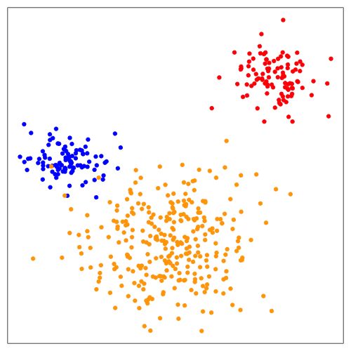
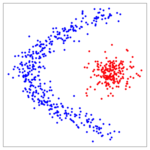
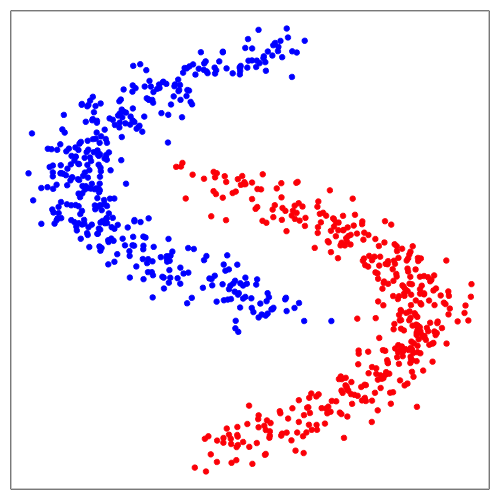
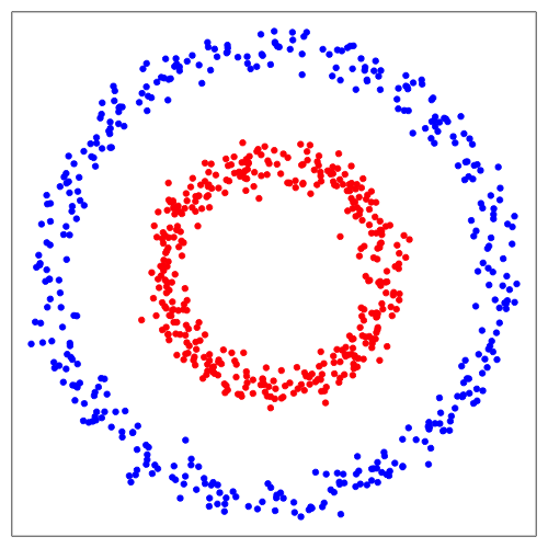
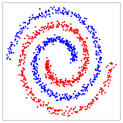
(a)                  (b)                  (c)                  (d)                  (e)

Figure 1: A few examples of different shapes of two-dimensional data. Different colors reflecting different data generating schemes: (a) three samples generated from three bivariate Gaussian distributions; (b) one sample from a bivariate Gaussian distribution and the other from a parabola with perturbations; (c) two parabolas with perturbations; (d) two rings with perturbations; and (e) two logarithmic spirals with perturbations.

Figure 1 colors them in their data generating schemes. Two classical clustering algorithms are applied to these data: the standard $k$-means clustering algorithm (kmeans function in R) and the spectral clustering (specc function in R package kernlab). The clustering results are shown in Figure 2.

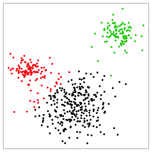
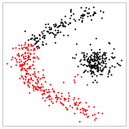
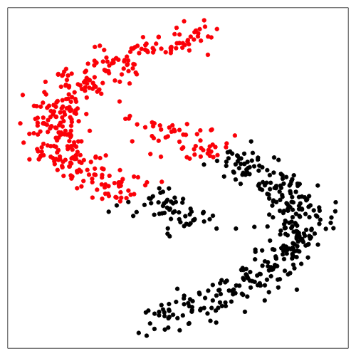
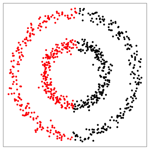
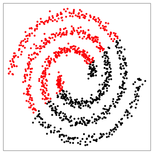
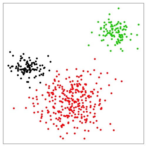
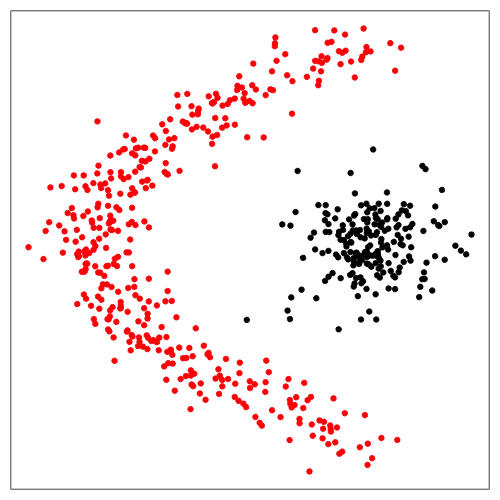
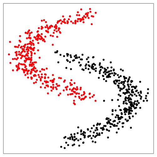
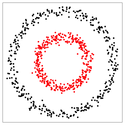
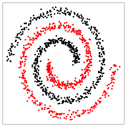
(a)                  (b)                  (c)                  (d)                  (e)

Figure 2: Clustering results based on the standard $k$-means approach (top row) and the spectral clustering (bottom row) for the five datasets in Figure 1.

It is clear that the clustering results based on the spectral clustering are much more satisfying. Hence, even though the definition of “similar” could be arbitrary in some sense, one probably wants to separate observations from different data generating schemes into different clusters. Generally speaking, cluster analysis is useful when the data set consists of mixture of observations from different underlying data generating schemes/models, and we would like to partition the observations into different clusters such that each cluster could be modeled simply, such as using a function or a distribution, so that we could summarize the dataset in a concise way and/or implement different treatments to different clusters according to their properties. In the above examples, the $k$-means approach minimizes the within-cluster sum of square (place ‘similar’ points together to some extent); however, it does not make the followup task – to understand the observations in each cluster – easier, and thus not useful.

In the following, we refer to points that could be represented by a relatively simple distribution/model as one cluster, and our goal is to group observations that are similar in underlying distribution/model.

1.2 Difficulties in clustering high-dimensional data

In Section 1.1, the spectral clustering does a good job in all examples. However, when the dimension of the data becomes high, this would no longer be the case. Consider a simple situation that the data is a mixture of observations from two distributions, $\mathcal{N}_{d}(\mathbf{0},\Sigma)$ and $\mathcal{N}_{d}(a\mathbf{1},b\Sigma)$, $d=200$, $\Sigma_{ij}=0.1^{|i-j|}$, where $\Sigma_{ij}$ is the $(i,j)$th element of $\Sigma$. Suppose there are 50 observations in each cluster and the goal is to separate them. Consider two simulation settings:

• Setting 1 (only mean differs): $a=0.25$, $b=1$.

• Setting 2 (both mean and variance differ): $a=0.25$, $b=1.8$.

We apply spectral clustering to data generated from the two settings and the mis-clustering rates on a typical simulation run are shown in Table 1. We see that when there is an additional variance difference, the mis-clustering rate is even higher than when there is only mean difference. We also apply some currently popular clustering methods. Influential Feature-PCA (IF-PCA) was introduced by Jin and Wang (2016) and achieve notable successes in clustering gene microarray data. $t$-SNE ($t$-distributed stochastic neighbor embedding) (Maaten and Hinton, 2008) was initially proposed for data visualization by projecting observations into a two-dimensional space. It effectively brings “similar” observations closer together in this two-dimensional space and thus attracts attentions in the area of cluster analysis. Mwangi, Soares and Hasan (2014) suggested employing the $k$-means clustering algorithm on the two-dimensional projected data derived from $t$-SNE. The mis-clustering rates of these methods are also presented in Table 1.

Table 1: Mis-clustering rate estimated from 50 simulation runs with the number in the parentheses the estimated standard deviation. The smallest mis-clustering rate under each setting is in bold.

	Spectral	IF-PCA	$t$-SNE
Setting 1	0.282 (0.107)	0.359 (0.082)	0.304 (0.109)
Setting 2	0.466 (0.025)	0.379 (0.083)	0.466 (0.027)

Setting 1 is a relatively easy case that the two clusters differ only in their means. We see that the spectral clustering shows clear advantage over the other candidates in this relatively easy scenario. Setting 2 is more complicated that the two clusters differ in scale in addition to the mean difference. We see that IF-PCA and $t$-SNE show worse performance than setting 1. The spectral clustering fails under this setting as well. For the spectral clustering, it is closely related to the Mincut problem if the observations are represented through a similarity graph. When the dimension is high and the two clusters differ in scale, due to the curse of dimensionality, the observations in the cluster with a larger variance would be much more sparsely scattered than those in the cluster with a smaller variance. As a result, for any observation in the cluster with a larger variance, its nearest points tend to be from the other cluster, causing the spectral clustering to fail. We explore this phenomenon more next.

1.3 Patterns in high dimensions

We here explore how the curse of dimensionality kicks in. Figure 3 plots the average probabilities of observations in sample 1 and sample 2 that find $k$ nearest neighbors within the sample, respectively. If a $k$-nearest neighbor ($k$-NN) graph on the pooled observations is constructed that each observation points to its first $k$ nearest neighbors, then $p_{11}$ is defined as the number of edges in the graph that point from an observation in sample 1 to another observation in sample 1 divided by the total number of edges that point from an observation in sample 1, and $p_{22}$ is defined as the number of edges in the graph that point from an observation in sample 2 to another observation in sample 2 divided by the total number of edges in the graph that point from an observation in sample 2. Here, sample 1 contains $m$ observations randomly generated from $\mathcal{N}_{d}(\mathbf{0},\Sigma)$, and sample 2 contains $n$ observations randomly generated from $\mathcal{N}_{d}(a\mathbf{1},b\Sigma)$, where $d=200$, $\Sigma_{ij}=0.1^{|i-j|}$. We consider three settings:

• Setting 0 (same distribution): $a=0$, $b=1$.

• Setting 1 (mean differs): $a=0.3$, $b=1$.

• Setting 2 (mean and variance differ): $a=0.3$, $b=1.3$.

Figure 3: Plots of $p_{11}$ (black) and $p_{22}$ (blue) considering $k$ nearest neighbors under different settings. The dashed lines are the base level when the two clusters are from the same distribution $p_{11}^{(0)}=(m-1)/(N-1)$ (black dashed line) and $p_{22}^{(0)}=(n-1)/(N-1)$ (blue dashed line). The two dashed lines overlap with each other when $m=n$.

When the two samples are from the same distribution, the probability one observation finds another observation to be among its first $k$ nearest neighbors is always $k/(N-1)$. Let $p_{11}^{(0)}$ and $p_{22}^{(0)}$ be the expectations of $p_{11}$ and $p_{22}$ when the two samples are from the same distribution, then $p_{11}^{(0)}=(m-1)/(N-1)$ and $p_{22}^{(0)}=(n-1)/(N-1)$. Under setting 0, we see that $p_{11}$ and $p_{22}$ are close to $p_{11}^{(0)}$ and $p_{22}^{(0)}$, respectively, across all $k$’s.

When the two samples are from different distributions with mean difference, we see that $p_{11}$ and $p_{22}$ are larger than $p_{11}^{(0)}$ and $p_{22}^{(0)}$, respectively, until at $k=N-1$ where each observation finds every other observations as its first $N-1$ nearest neighbors. This is what we would expect.

When the two distributions differ in scale, we see that $p_{11}$ is still larger than $p_{11}^{(0)}$ in general, but $p_{22}$ is smaller than $p_{22}^{(0)}$ across all $k$’s. This is where the curse of dimensionality kicks in. Here, $d=200$ and sample 2 is from a distribution with a larger variance than that of sample 1. Since the volume of the space grows exponential in dimension, observations in sample 2 tends to find observations in sample 1 to be closer than other observations in sample 2.

In this paper, we take the above phenomenon into account and propose a new clustering criteria based on some theoretical results (Section 2). The new method is compared with existing methods under a variety of settings in Section 3 and applied to real data applications in Section 4. The paper concludes with discussions in Section 5.

2 Proposed method

2.1 Notations

We use $G_{k}$ to denote the set of edges in $k$-NN, and $(i,j)\in G_{k}$ if node $i$ points to node $j$ (each node points to its first $k$ nearest neighbors). Let $x$ be an $N$-length vector of 1’s and 0’s, and

$$R_{1,k}(x) =\sum_{(i,j)\in G_{k}}I_{x_{i}=x_{j}=1},\quad R_{2,k}(x)=\sum_{(i,j)\in G_{k}}I_{x_{i}=x_{j}=0}.$$

Then, $x$ divides the observations into two clusters: 1’s (Cluster 1) and 0’s (Cluster 2). Let $m$ be the number of 1’s in $x$ and $n$ be the number of 0’s in $x$. Let $p_{11,k}(x)$ be one $k$th of the probability that an observation in cluster 1 defined by $x$ finds another observation in cluster 1 to be one of its first $k$ nearest neighbors, i.e., $p_{11,k}(x)=R_{1,k}(x)/(km)$. Similarly, $p_{12,k}(x)=(km-R_{1,k}(x))/(km)$, $p_{21,k}(x)=R_{2,k}(x)/(kn)$, $p_{22,k}(x)=(kn-R_{2,k}(x))/(kn)$. It is clear that

$$p_{11,k}(x)+p_{12,k}(x)=1,\quad p_{21,k}(x)+p_{22,k}(x)=1.$$

Let $x^{*}$ represents the true clustering, and there are $m^{*}$ 1’s in $x^{*}$ and $n^{*}$ 0’s in $x^{*}$ ($m^{*}+n^{*}=N$). We define $p_{11}^{(0)}$ and $p_{22}^{(0)}$ to be the expected values of $p_{11,k}$ and $p_{22,k}$ when the two clusters are from the same distribution, i.e.,

$$p_{11}^{(0)}=\tfrac{m^{*}-1}{N-1},\quad p_{22}^{(0)}=\tfrac{n^{*}-1}{N-1}.$$

2.2 New clustering criteria

If the two clusters are indeed from two different distributions, we would have the following three possible scenarios for some $k$’s according to Section 1.3:

1. $p_{11,k}(x^{*})>p_{11}^{(0)}$, $p_{22,k}(x^{*})>p_{22}^{(0)}$,

2. $p_{11,k}(x^{*})>p_{11}^{(0)}$, $p_{22,k}(x^{*})<p_{22}^{(0)}$,

3. $p_{11,k}(x^{*})<p_{11}^{(0)}$, $p_{22,k}(x^{*})>p_{22}^{(0)}$.

From Figure 3, $p_{11,k}(x^{*})$ and $p_{22,k}(x^{*})$ depend on $k$. Here, we first fix $k$ and discuss the clustering criteria with the hope to find $x^{*}$. We then discuss the choice of $k$ in Section 2.3. For notation simplicity, we use $R_{1}(x)$ and $R_{2}(x)$ instead of $R_{1,k}(x)$ and $R_{2,k}(x)$ in the rest of this section.

We borrow strengths from graph-based two-sample tests (Chen and Friedman, 2017) and propose to use the following two quantities:

$$Z_{w}(x) =\tfrac{R_{w}(x)-\mu_{w}(x)}{\sigma_{w}(x)},\quad R_{w}(x)=\tfrac{n-1}{N-2}R_{1}(x)+\tfrac{m-1}{N-2}R_{2}(x),$$

$$Z_{d}(x) =\tfrac{R_{d}(x)-\mu_{d}(x)}{\sigma_{d}(x)},\quad R_{d}(x)=R_{1}(x)-R_{2}(x),$$

where $\mu_{w}(x)$, $\sigma_{w}(x)$, $\mu_{d}(x)$, $\sigma_{d}(x)$ are normalizing terms so that $Z_{w}(x)$ and $Z_{d}(x)$ are properly standardized to mean 0 and variance 1 if there is only one cluster. Their expressions can be obtained through similar treatments under the two-sample testing setting (Schilling, 1986; Henze, 1988) and the change-point detection setting (Liu and Chen, 2022). Let $\mathcal{X}_{m}$ be the set of all $x$’s with $m$ 1’s and $(N-m)=n$ 0’s. Then, for $x\in\mathcal{X}_{m}$, we have,

$$\mu_{w}(x) =\tfrac{(m-1)(n-1)}{(N-1)(N-2)}kN,$$

$$\sigma_{w}(x) =\tfrac{mn(m-1)(n-1)}{N(N-1)(N-2)(N-3)}\left(kN+q_{1,k}-\tfrac{1}{N-2}(q_{2,k}+kN-k^{2}N)-\tfrac{2}{N-1}k^{2}N\right),$$

$$\mu_{d}(x) =k(m-n),$$

$$\sigma_{d}(x) =\tfrac{mn}{N(N-1)}(q_{2,k}+kN-k^{2}N).$$

where $q_{1,k}=\sum_{(i,j)\in G_{k}}I_{(j,i)\in G_{k}}$, $q_{2,k}=\sum_{i=1}^{N}\sum_{j\neq l}I_{(j,i),(l,i)\in G_{k}}$.

Define $\textsf{E}_{2}(\cdot)$ be the expectation under the fact that there are two clusters.

Theorem 1.

For any fixed $k$, if $p_{11,k}(x^{*})$ and $p_{22,k}(x^{*})$ belong to any of the three scenarios, we have:

• Under scenario (1), $\textsf{E}_{2}(Z_{w}(x))$ is maximized at $x=x^{*}$ or $x=1-x^{*}$.

• Under scenario (2), $\textsf{E}_{2}(Z_{d}(x))$ is maximized at $x=x^{*}$.

• Under scenario (3), $\textsf{E}_{2}(Z_{d}(x))$ is maximized at $x=1-x^{*}$.

Based on the above theorem, we could use $\max_{x}Z_{w}(x)$ to cluster scenario (1), and use $\max_{x}Z_{d}(x)$ to cluster scenarios (2) and (3). However, in reality, we won’t know which scenario it is, so we propose to use

$$M_{\kappa}(x)=\max(Z_{w}(x),\kappa Z_{d}(x))$$

as the criterion. The choice of $\kappa$ is discussed in Section 2.4 and $\kappa=1.55$ is set as the default choice. Table 2 adds the mis-clustering rate of the new method to Table 1. We see that the mis-clustering rate of the new method under setting 1 is on par with the best remaining methods, and the mis-clustering rate of the new method under setting 2 is much lower than all other methods.

Table 2: Mis-clustering rate under the same settings as in Table 1.

	Spectral	IF-PCA	$t$-SNE	New
Setting 1	0.282 (0.107)	0.359 (0.082)	0.304 (0.109)	0.258 (0.166)
Setting 2	0.466 (0.025)	0.379 (0.083)	0.466 (0.027)	0.003 (0.006)

Remark 1.

It can also be shown that, under scenario (1), $\textsf{E}_{2}(R_{w}(x))-\mu_{w}(x)$ is maximized at $x=x^{*}$ or $x=1-x^{*}$; under scenario (2), $\textsf{E}_{2}(R_{d}(x))-\mu_{d}(x)$ is maximized at $x=x^{*}$; under scenario (3), $\textsf{E}_{2}(R_{d}(x))-\mu_{d}(x)$ is maximized at $x=1-x^{*}$. However, we do not recommended to use $R_{w}(x)-\mu_{w}(x)$ and $R_{d}(x)-\mu_{d}(x)$ as the criteria as they are not well normalized and hard to be combined together if one does not know which scenario the actual data falls in.

Proof of Theorem 1.

We first compute $\textsf{E}_{2}(R_{w}(x))$ and $\textsf{E}_{2}(R_{d}(x))$. For $x$, suppose there are $\Delta_{1}\in[0,m^{*}]$ observations in cluster 1 placed into cluster 2, and $\Delta_{2}\in[0,n^{*}]$ observations in cluster 2 placed into cluster 1. So $x\in\mathcal{X}_{m}$ with $m=m^{*}-\Delta_{1}+\Delta_{2}$. Since $k$ is fixed here, for simplicity, we denote $p_{11,k}(x^{*})$, $p_{12,k}(x^{*})$, $p_{21,k}(x^{*})$, $p_{22,k}(x^{*})$ by $p_{11}^{*}$, $p_{12}^{*}$, $p_{21}^{*}$, $p_{22}^{*}$, respectively. Then, we have,

$$\textsf{E}_{2}(R_{1}(x)) =p_{11}^{*}km^{*}\tfrac{(m^{*}-\Delta_{1})(m^{*}-\Delta_{1}-1)}{m^{*}(m^{*}-1)}+p_{12}^{*}km^{*}\tfrac{(m^{*}-\Delta_{1})\Delta_{2}}{m^{*}n^{*}}$$

$$\quad+p_{21}^{*}kn^{*}\tfrac{(m^{*}-\Delta_{1})\Delta_{2}}{m^{*}n^{*}}+p_{22}kn^{*}\tfrac{\Delta_{2}(\Delta_{2}-1)}{n^{*}(n^{*}-1)},$$

$$\textsf{E}_{2}(R_{2}(x)) =p_{22}^{*}kn^{*}\tfrac{(n^{*}-\Delta_{2})(n^{*}-\Delta_{2}-1)}{n^{*}(n^{*}-1)}+p_{21}^{*}kn^{*}\tfrac{(n^{*}-\Delta_{2})\Delta_{1}}{n^{*}m^{*}}$$

$$\quad+p_{12}^{*}km^{*}\tfrac{(n^{*}-\Delta_{2})\Delta_{1}}{n^{*}m^{*}}+p_{11}^{*}km^{*}\tfrac{\Delta_{1}(\Delta_{1}-1)}{m^{*}(m^{*}-1)}.$$

Then,

$$\textsf{E}_{2}(R_{w}(x)) =\tfrac{n^{*}+\Delta_{1}-\Delta_{2}-1}{N-2}\textsf{E}_{2}(R_{1}(x))+\tfrac{m^{*}-\Delta_{1}+\Delta_{2}-1}{N-2}\textsf{E}_{2}(R_{2}(x))$$

$$=k\tfrac{m^{*}(n^{*}-1)p_{11}^{*}+n^{*}(m^{*}-1)p_{22}^{*}}{N-2}$$

$$\quad+k\tfrac{m^{*}(n^{*}-1)p_{11}^{*}+n^{*}(m^{*}-1)p_{22}^{*}-N(m^{*}-1)}{m^{*}(m^{*}-1)(N-2)}\Delta_{1}^{2}$$

$$\quad+k\tfrac{m^{*}(n^{*}-1)p_{11}^{*}+n^{*}(m^{*}-1)p_{22}^{*}-N(n^{*}-1)}{n^{*}(n^{*}-1)(N-2)}\Delta_{2}^{2}$$

$$\quad+2k\tfrac{m^{*}(n^{*}-1)p_{11}^{*}+n^{*}(m^{*}-1)p_{22}^{*}+N}{m^{*}n^{*}(N-2)}\Delta_{1}\Delta_{2}$$

$$\quad-k\Delta_{1}\tfrac{(2m^{*}-1)(m^{*}(n^{*}-1)p_{11}^{*}+n^{*}(m^{*}-1)*p_{22}^{*})-N(m^{*}-1)^{2}}{m^{*}(m^{*}-1)(N-2)}$$

$$\quad-k\Delta_{2}\tfrac{(2n^{*}-1)(m^{*}(n^{*}-1)p_{11}^{*}+n^{*}(m^{*}-1)*p_{22}^{*})-N(n^{*}-1)^{2}}{n^{*}(n^{*}-1)(N-2)},$$

$$\textsf{E}_{2}(R_{d}(x)) =\textsf{E}_{2}(R_{1}(x))-\textsf{E}_{2}(R_{2}(x))$$

$$=p_{11}^{*}km^{*}-p_{22}^{*}kn^{*}-k\Delta_{1}\left(p_{11}^{*}-\tfrac{n^{*}}{m^{*}}p_{22}^{*}+\tfrac{N}{m^{*}}\right)$$

$$\quad+k\Delta_{2}\left(p_{22}^{*}-\tfrac{m^{*}}{n^{*}}p_{11}^{*}+\tfrac{N}{n^{*}}\right).$$

We start with $\textsf{E}_{2}(Z_{d}(x))$ as it is relatively simpler and some of the intermediate results can be used for $\textsf{E}_{2}(Z_{w}(x))$. Notice that

$$\textsf{E}_{2}(R_{d}(x))-\mu_{d}(x) =p_{11}^{*}km^{*}-p_{22}^{*}kn^{*}-k(m-n)$$

$$\quad-k\Delta_{1}\left(p_{11}^{*}-\tfrac{n^{*}}{m^{*}}p_{22}^{*}+\tfrac{N}{m^{*}}\right)+k\Delta_{2}\left(p_{22}^{*}-\tfrac{m^{*}}{n^{*}}p_{11}^{*}+\tfrac{N}{n^{*}}\right)$$

$$=k(p_{11}^{*}m^{*}-p_{22}^{*}n^{*}-(m^{*}-n^{*}))$$

$$\quad-k\Delta_{1}\left(p_{11}^{*}-\tfrac{n^{*}}{m^{*}}p_{22}^{*}+\tfrac{N}{m^{*}}-2\right)$$

$$\quad+k\Delta_{2}\left(p_{22}^{*}-\tfrac{m^{*}}{n^{*}}p_{11}^{*}+\tfrac{N}{n^{*}}-2\right)$$

$$=(p_{11}^{*}m^{*}-p_{22}^{*}n^{*}-(m^{*}-n^{*}))k\left(1-\tfrac{\Delta_{1}}{m^{*}}-\tfrac{\Delta_{2}}{n^{*}}\right).$$

Then

$$\textsf{E}_{2}(Z_{d}(x)) =\frac{\textsf{E}_{2}(R_{d}(x))-\mu_{d}(x)}{\sigma_{d}(x)}=(p_{11}^{*}m^{*}-p_{22}^{*}n^{*}-(m^{*}-n^{*}))kf_{d}(\Delta_{1},\Delta_{2}),$$

where

$$f_{d}(\Delta_{1},\Delta_{2}) =\tfrac{1-\frac{\Delta_{1}}{m^{*}}-\frac{\Delta_{2}}{n^{*}}}{\sqrt{(m^{*}-\Delta_{1}+\Delta_{2})(n^{*}+\Delta_{1}-\Delta_{2})}}.$$

Note that

$$\tfrac{\partial f_{d}}{\partial\Delta_{1}} =-\tfrac{N}{2m^{*}n^{*}}\tfrac{(n^{*}-\Delta_{2})(m^{*}-\Delta_{1}+2\Delta_{2})+\Delta_{1}\Delta_{2}}{(m^{*}-\Delta_{1}+\Delta_{2})^{1.5}(n^{*}+\Delta_{1}-\Delta_{2})^{1.5}}<0,$$

$$\tfrac{\partial f_{d}}{\partial\Delta_{2}} =-\tfrac{N}{2m^{*}n^{*}}\tfrac{(m^{*}-\Delta_{1})(n^{*}-\Delta_{2}+2\Delta_{1})+\Delta_{1}\Delta_{2}}{(m^{*}-\Delta_{1}+\Delta_{2})^{1.5}(n^{*}+\Delta_{1}-\Delta_{2})^{1.5}}<0.$$

So $f_{d}(\Delta_{1},\Delta_{2})$ achieves its maximum when $\Delta_{1}=\Delta_{2}=0$ with the maximum being $\frac{1}{\sqrt{m^{*}n^{*}}}$, and achieve its minimum when $\Delta_{1}=m^{*},\Delta_{2}=n^{*}$ with the minimum being $-\frac{1}{\sqrt{m^{*}n^{*}}}$. Also note that, under scenario (2), we have

$$p_{11}^{*}m^{*}-p_{22}^{*}n^{*}-(m^{*}-n^{*})>\frac{m^{*}-1}{N-1}m^{*}-\frac{n^{*}-1}{N-1}n^{*}-(m^{*}-n^{*})=0,$$

and under scenario (3), we have

$$p_{11}^{*}m^{*}-p_{22}^{*}n^{*}-(m^{*}-n^{*})<0.$$

Therefore, under scenario (2), $\textsf{E}_{2}(Z_{d}(x))$ is maximized when $\Delta_{1}=\Delta_{2}=0$, i.e., at $x=x^{*}$; and under scenario (3), $\textsf{E}_{2}(Z_{d}(x))$ is maximized when $\Delta_{1}=m^{*},\Delta_{2}=n^{*}$, i.e., at $x=1-x^{*}$.

Now, we move onto $\textsf{E}_{2}(Z_{w}(x))$. We first compute $\textsf{E}_{2}(R_{w}(x))-\mu_{w}(x)$:

$$\textsf{E}_{2} (R_{w}(x))-\mu_{w}(x)$$

$$=k\tfrac{m^{*}(n^{*}-1)p_{11}^{*}+n^{*}(m^{*}-1)p_{22}^{*}-\frac{(m^{*}-1)(n^{*}-1)N}{N-1}}{N-2}$$

$$\quad+k\tfrac{m^{*}(n^{*}-1)p_{11}^{*}+n^{*}(m^{*}-1)p_{22}^{*}-\frac{(m^{*}-1)(n^{*}-1)N}{N-1}}{m^{*}(m^{*}-1)(N-2)}\Delta_{1}^{2}$$

$$\quad+k\tfrac{m^{*}(n^{*}-1)p_{11}^{*}+n^{*}(m^{*}-1)p_{22}^{*}-\frac{(m^{*}-1)(n^{*}-1)N}{N-1}}{n^{*}(n^{*}-1)(N-2)}\Delta_{2}^{2}$$

$$\quad+2k\tfrac{m^{*}(n^{*}-1)p_{11}^{*}+n^{*}(m^{*}-1)p_{22}^{*}\frac{(m^{*}-1)(n^{*}-1)N}{N-1}}{m^{*}n^{*}(N-2)}\Delta_{1}\Delta_{2}$$

$$\quad-k\Delta_{1}\tfrac{(2m^{*}-1)\left(m^{*}(n^{*}-1)p_{11}^{*}+n^{*}(m^{*}-1)p_{22}^{*}-\frac{(m^{*}-1)(n^{*}-1)N}{N-1}\right)}{m^{*}(m^{*}-1)(N-2)}$$

$$\quad-k\Delta_{2}\tfrac{(2n^{*}-1)\left(m^{*}(n^{*}-1)p_{11}^{*}+n^{*}(m^{*}-1)p_{22}^{*}-\frac{(m^{*}-1)(n^{*}-1)N}{N-1}\right)}{n^{*}(n^{*}-1)(N-2)}$$

$$=k\tfrac{m^{*}(n^{*}-1)p_{11}^{*}+n^{*}(m^{*}-1)p_{22}^{*}-\frac{(m^{*}-1)(n^{*}-1)N}{N-1}}{N-2}$$

$$\quad\times\left(1+\tfrac{\Delta_{1}^{2}}{m^{*}(m^{*}-1)}+\tfrac{\Delta_{2}^{2}}{n^{*}(n^{*}-1)}+\tfrac{2\Delta_{1}\Delta_{2}}{m^{*}n^{*}}-\tfrac{(2m^{*}-1)\Delta_{1}}{m^{*}(m^{*}-1)}-\tfrac{(2n^{*}-1)\Delta_{2}}{n^{*}(n^{*}-1)}\right).$$

Then

$$\textsf{E}_{2}(Z_{w}(x)) =k\tfrac{m^{*}(n^{*}-1)p_{11}^{*}+n^{*}(m^{*}-1)p_{22}^{*}-\frac{(m^{*}-1)(n^{*}-1)N}{N-1}}{N-2}f_{w}(\Delta_{1},\Delta_{2}),$$

where

$$f_{w}(\Delta_{1},\Delta_{2}) =\tfrac{1+\frac{\Delta_{1}^{2}}{m^{*}(m^{*}-1)}+\frac{\Delta_{2}^{2}}{n^{*}(n^{*}-1)}+\frac{2\Delta_{1}\Delta_{2}}{m^{*}n^{*}}-\frac{(2m^{*}-1)\Delta_{1}}{m^{*}(m^{*}-1)}-\frac{(2n^{*}-1)\Delta_{2}}{n^{*}(n^{*}-1)}}{\sqrt{(m^{*}-\Delta_{1}+\Delta_{2})(n^{*}+\Delta_{1}-\Delta_{2})(m^{*}-\Delta_{1}+\Delta_{2}-1)(n^{*}+\Delta_{1}-\Delta_{2}-1)}}.$$

It’s complicated to work on $f_{w}$ directly. Here, we first consider

$$\tilde{f}_{d}(\Delta_{1},\Delta_{2}) =\tfrac{1-\frac{\Delta_{1}}{m^{*}-1}-\frac{\Delta_{2}}{n^{*}-1}}{\sqrt{(m^{*}-\Delta_{1}+\Delta_{2}-1)(n^{*}+\Delta_{1}-\Delta_{2}-1)}}.$$

With similar arguments as for $f_{d}(\Delta_{1},\Delta_{2})$, we know that, for $\Delta_{1}\in[0,m^{*}-1],\Delta_{2}\in[0,n^{*}-1]$, $\tilde{f}_{d}(\Delta_{1},\Delta_{2})$ achieves its maximum when $\Delta_{1}=\Delta_{2}=0$ with the maximum being $\frac{1}{\sqrt{(m^{*}-1)(n^{*}-1)}}$, and achieve its minimum when $\Delta_{1}=m^{*}-1,\Delta_{2}=n^{*}-1$ with the minimum being $-\frac{1}{\sqrt{(m^{*}-1)(n^{*}-1)}}$. For the three corner cases $(\Delta_{1}=m^{*}-1,\Delta_{2}=n^{*})$, $(\Delta_{1}=m^{*},\Delta_{2}=n^{*}-1)$, $(\Delta_{1}=m^{*},\Delta_{2}=n^{*})$, we discuss slightly later.

Hence, for $\Delta_{1}\in[0,m^{*}-1],\Delta_{2}\in[0,n^{*}-1]$, we have $f_{d}(\Delta_{1},\Delta_{2})\tilde{f}_{d}(\Delta_{1},\Delta_{2})$ achieves its maximum at $\Delta_{1}=\Delta_{2}=0$ and $\Delta_{1}=m^{*}-1,\Delta_{2}=n^{*}-1$ with the maximum $\frac{1}{\sqrt{m^{*}n^{*}(m^{*}-1)(n^{*}-1)}}$.

Notice that

$$f_{w}(\Delta_{1},\Delta_{2}) =f_{d}(\Delta_{1},\Delta_{2})\tilde{f}_{d}(\Delta_{1},\Delta_{2})-h(\Delta_{1},\Delta_{2}),$$

where

$$h(\Delta_{1},\Delta_{2})=\tfrac{\frac{N-2}{m^{*}n^{*}(m^{*}-1)(n^{*}-1)}\Delta_{1}\Delta_{2}}{\sqrt{(m^{*}-\Delta_{1}+\Delta_{2})(n^{*}+\Delta_{1}-\Delta_{2})(m^{*}-\Delta_{1}+\Delta_{2}-1)(n^{*}+\Delta_{1}-\Delta_{2}-1)}}.$$

Here, the $h(\Delta_{1},\Delta_{2})>0$ when $\Delta_{1}\Delta_{2}>0$, so $f_{w}(0,0)>f_{w}(m^{*}-1,n^{*}-1)$. For the three left out corner cases, we have

• $f_{w}(m^{*},n^{*})=\frac{1}{\sqrt{n^{*}m^{*}(n^{*}-1)(m^{*}-1)}}=f_{w}(0,0)$.

• $f_{w}(m^{*},n^{*}-1)=\frac{1-\frac{2}{n^{*}}}{\sqrt{(n^{*}-1)(m^{*}+1)(n^{*}-2)m^{*}}}=\frac{\sqrt{\left(1-\frac{2}{n^{*}}\right)\left(1-\frac{2}{m^{*}+1}\right)}}{\sqrt{n^{*}m^{*}(n^{*}-1)(m^{*}-1)}}<f_{w}(0,0)$.

• $f_{w}(m^{*}-1,n^{*})=\frac{1-\frac{2}{m^{*}}}{\sqrt{(n^{*}+1)(m^{*}-1)n^{*}(m^{*}-2)}}=\frac{\sqrt{\left(1-\frac{2}{m^{*}}\right)\left(1-\frac{2}{n^{*}+1}\right)}}{\sqrt{n^{*}m^{*}(n^{*}-1)(m^{*}-1)}}<f_{w}(0,0)$.

Hence, $f_{w}(\Delta_{1},\Delta_{2})$ achieves its maximum when $\Delta_{1}=\Delta_{2}=0$ or $\Delta_{1}=m^{*},\Delta_{2}=n^{*}$.

Under scenario (1),

$$m^{*}(n^{*}-1)p_{11}^{*}+n^{*}(m^{*}-1)p_{22}^{*}-\frac{(m^{*}-1)(n^{*}-1)N}{N-1}$$

$$\quad\quad>m^{*}(n^{*}-1)\frac{m^{*}-1}{N-1}+n^{*}(m^{*}-1)\frac{n^{*}-1}{N-1}-\frac{(m^{*}-1)(n^{*}-1)N}{N-1}=0.$$

So $\textsf{E}_{2}(Z_{d}(x))$ achieves its maximum when $\Delta_{1}=\Delta_{2}=0$ or $\Delta_{1}=m^{*},\Delta_{2}=n^{*}$, i.e., when $x=x^{*}$ or $x=1-x^{*}$.

∎

Given the results from Theorem 1, the next step is to find an efficient way to solve the optimization problem. Generally speaking, the optimization of $Z_{w}(x)$ or $Z_{d}(x)$ is an NP-hard problem. Instead of searching for the whole labels assignment space of this optimization problem, we address this task by a greedy algorithm. Suppose we are given an $\mathbf{x}$, which is an initial division vector of the clusters into two groups (could be randomly generated). We then find among all single changes to $\mathbf{x}$ that is defined as changing one element in $\mathbf{x}$ from $s$ to $1-s$, and choose the change that will give the biggest increase of the corresponding $Z_{w}$ (or $Z_{d}$). We keep making such moves until there is no increase available. We pick many initial values of the partition $\mathbf{x}$ and pick the result with the maximum value of $Z_{w}$ (or $Z_{d}$). Notice that at each step, we only make one element change of $\mathbf{x}$, it is not necessary to loop over the whole adjacency matrix to calculate $R_{1},R_{2}$ and $\sigma_{d},\sigma_{w}$ to update the value of $Z_{w}(x)$ and $Z_{d}(x)$. Instead, we can only check the edges related to the label switch to calculate the increase or decrease in $R_{1}$ and $R_{2}$. For $\sigma_{d},\sigma_{w}$, the only terms related to the optimization process are $m,n$, hence can be calculated easily during the updating procedure.

2.3 Choice of $k$

The first step of our clustering procedure is to construct $G_{k}$ ($k$-NN graph). Here, $k$ can be an arbitrary integer number between 1 and $N-1$. We can create all the possible $G_{k}$ and perform the clustering process. Typically, different values of $k$ lead to different clustering outcomes. As the underlying true partition of the clusters is usually not available, a natural question is how to choose $k$ such that the clustering criteria will have the optimal power or give us the most reasonable partition. In this section, we intend to use an empirical way to discuss the choice of $k$.

We want to choose $k$ such that $p_{11,k}(x^{*})$ and $p_{22,k}(x^{*})$ are far from $p_{11}^{(0)}$ and $p_{22}^{(0)}$, and at the same time there are enough edges in the graph that contribute to the evidence. Heuristically, when the value of $k$ is small, the graph is sparse and some useful similarity information among the individuals might not be fully captured by $Z_{w}$ and $Z_{d}$. On the other hand, when the value of $k$ is too large, it includes some irrelevant information. If there is groundtruth for a given dataset, then there always exist an (or a few) optimal choice of $k$ that will result in the partition which has the largest overlap with the underlying true group assignments.

The choice of the hyper-parameter $k$ under the two sample testing and change point detection regime for the statistic $Z_{w}$ and $Z_{d}$ was discussed in Zhu and Chen (2021), Zhang and Chen (2021) and Zhou and Chen (2022). Specifically, they consider the power of the methods for $k=[N^{\lambda}]$ when varying $\lambda$ from 0 to 1 in different settings.

Here, we explore the relation between $k$ and mis-clustering rate. In particular, we want to find out whether the $k$ that leads to the maximum value of $M_{\kappa}$ would result in the minimum clustering error. In each simulation setting, we generate the $k$-NN graphs for $k$ from 1 to $N-3$, increased by 2 at each time. Again, consider the Gaussian mixture example where we have two groups of samples from $\mathcal{N}_{d}(\mathbf{0},\Sigma)$ and $\mathcal{N}_{d}(a\mathbf{1},b\Sigma),\Sigma_{ij}=0.1^{|i-j|}$.

• Setting 1 (only mean differs): $a>0$, $b=1$.

• Setting 2 (only variance differs): $a=0,b>1$.

• Setting 3 (both mean and variance differ): $a>0,b>1$.

Figure 4: Values of $Z_{w}$, $Z_{d}$ and $M_{\kappa}$ (top panel) and mis-clustering rate (bottom panel) over $k$. $m=n=50$.

We first examine the values of $Z_{w}$ and $Z_{d}$ for different settings, along with the value of $M_{\kappa}$ with $\kappa=1.55$, i.e., $M_{\kappa}(x)=\max(Z_{w}(x),1.55Z_{d}(x))$. The choice of $\kappa$ is discussed in Section 2.4. Note that we here concern the value of $k$ that leads to the maximum $M_{\kappa}$ and the value of $\kappa$ does not affect this choice of $k$ as long as $\kappa$ is within a certain range. We set the dimension to be $d=800$ here. For the cluster sizes, we examine both balanced ($m=n=50$) and unbalanced ($m=30,n=70$) cases.

Figure 4 plots the values of $Z_{w}$, $Z_{d}$ and $M_{\kappa}$ over $k$ under all three settings for the balanced case (top panel), as well as the mis-clustering rate (bottom panel). We see that the mis-clustering rate reaches its minimum when $M_{\kappa}$ is at its maximum in all settings. The same pattern also appears for the unbalanced case (Figure 5). This finding is particularly fascinating since $M_{\kappa}$ over various $k$ values is entirely observable from the given data, allowing us to simply select the $k$ that maximizes $M_{\kappa}$. In practice, we consider only $k\leq 0.9N$ for computational considerations, as we never observe the lowest mis-clustering rate attained at an exceedingly large value of $k$.

Figure 5: Values of $Z_{w}$, $Z_{d}$ and $M_{\kappa}$ (top panel) and mis-clustering rate (bottom panel) over $k$. $m=30,n=70$.

2.4 Choice of $\kappa$

From Section 2.2, $\max_{x}Z_{w}(x)$ can be used to cluster scenario (1) and $\max_{x}Z_{d}(x)$ is suitable for scenarios (2) and (3). Due to the fact that we don’t know which scenario we are dealing with in reality, $M_{\kappa}(x)=\max(Z_{w}(x),\kappa Z_{d}(x))$ was proposed for these three scenarios. We here discuss the choice of $\kappa$. Ideally, when the scenario is (1), we would like $Z_{w}$ to dominate in $M_{\kappa}$; while when the scenario is (2) or (3), we would like $Z_{d}$ to dominate in $M_{\kappa}$. However, this dominance does not need to hold for all $k$’s. Instead, as long as $M_{\kappa}$ picks the correct quantity ($Z_{w}$ or $Z_{d}$) when the correct quantity reaches its maximum, the goal is achieved given how we choose $k$. This can be seen clearly from Figure 4 and 5. In Figure 4 and 5, the leftmost pictures, two clusters are generated from $\mathcal{N}_{d}(\mathbf{0},\Sigma)$ and $\mathcal{N}_{d}(a\mathbf{1},\Sigma)$. It belongs to scenario (1) according to Figure 3 and $Z_{w}$ should then dominate $M_{\kappa}$ based on the statements above. We see that $M_{\kappa}$ is identical with $Z_{w}$ when $Z_{w}$ reach its maximum but differs from $Z_{w}$ in boundaries. That will not affect the mis-clustering rate using $M_{\kappa}$ given how we choose $k$. With the above observations, we use the following simulation study to choose $\kappa$. All other parameters remain the same as in Figure 4 setting 1 (only mean differs), we gradually increase the location difference parameter $a$ to determine the upper bound of $\kappa$. All other parameters remain the same as in Figure 4 setting 2 (only variance differs), we gradually increase the scale difference parameter $b$ to determine the lower bound of $\kappa$. For each setting, we run 50 times.

Figure 6: Plots of ratio ($r=Z_{w}/Z_{d}$), versus the signal strength. Left panel: location difference, $b=1$, $a$ increases from 0.05 to 0.3. Blue dash line $r=1.8$ is the minimum value of the boxplot when $a=0.2$. “mis_rate” is the mean mis-clustering rate of using $Z_{w}$ as criterion, with green indicating higher errors and orange indicating lower errors; Right panel: scale difference, $a=0$, $b$ increases from 1.05 to 1.3. Red dash line $r=1.3$ is the maximum value of the boxplot when $b=1.15$, “mis_rate” is the mean mis-clustering rate of using $Z_{d}$ as criterion, green indicating higher errors and orange lower error.

In Figure 6, left panel, the mis-clustering rate has a huge decrease at around $a=0.2$. When the signal is less than this threshold, the difference between these two clusters are not big enough for the algorithm to distinguish them (close to 0.5 misclustering rate). After this phase transition, the misclustering rate is much smaller. Hence, we would want $Z_{w}$ to dominate in $M_{\kappa}$ when $a\geq 0.2$, i.e., to choose $\kappa$ smaller than the ratio when $a\geq 0.2$. This leads to an upper bound for $\kappa$, which is the minimum value of the boxplot at $a=0.2$. With a similar argument, for the right panel, we would want $Z_{d}$ to dominate in $M_{\kappa}$ when $b\geq 1.15$. This leads to a lower bound for $\kappa$, which is the maximum value of the boxplot at $b=1.15$. Then, a proper choice of $\kappa$ would be in between the upper bound $r=1.8$ and the lower bound $r=1.3$. For simplicity, we choose the middle point $\kappa=1.55$ as our default choice. While we want to note here that if one has a prior probability on the three scenarios that a particular problem would belong to, then the choice of $\kappa$ could be adjusted to favor more on $Z_{w}$ or $Z_{d}$ accordingly.

3 Numerical studies

In this section, we compare the performance of the new methods with other existing methods on synthetic data. To be more specific, we compare the following methods:

• Spectral: Spectral clustering in Hastie et al. (2009).

• IF-PCA: influential feature PCA proposed by Jin and Wang (2016).

• $t$-SNE: using $t$-SNE to project the data into the two dimensional space and then using k-means clustering algorithm on the projected data (Mwangi, Soares and Hasan, 2014).

We consider a few different settings.

• Gaussian mixture: $\mathcal{N}_{d}(\mathbf{0},\Sigma)$ and $\mathcal{N}_{d}(a\mathbf{1},b\Sigma)$, $\Sigma_{ij}=0.1^{|i-j|}$. The location parameter $a\in\{0,0.25,0.5\}$ and the scale parameter $b\in\{1,1.4,1.8\}$.

• t-distribution mixture: $t_{10}(\mathbf{0},\Sigma)$ and $t_{10}(a\mathbf{1},b\Sigma)$, $\Sigma_{ij}=0.1^{|i-j|}$. The location parameter $a\in\{0,0.4,0.8\}$ and the scale parameter $b\in\{1,1.4,1.8\}$.

• Log-normal mixture: $\text{lognormal}(\mathbf{0},\Sigma)$ and $\text{lognormal}(a\mathbf{1},\Sigma)$, $\Sigma_{ij}=0.9^{|i-j|}$. The parameters $a\in\{0.7,0.8,0.9\}$.

Figure 7: Mis-clustering for Gaussian mixtures $\mathcal{N}_{d}(\mathbf{0},\Sigma)$ and $\mathcal{N}_{d}(a\mathbf{1},b\Sigma)$.

For each setting, the misclustering rate is estimated through 50 simulation runs. Figure 7, column 1, presents the results for traditional location difference Gaussian Mixture with a fixed covariance matrix. The top panel portrays a relatively mild difference between the clusters with $a=0.25$ while the bottom panel depicts a larger difference with $a=0.5$. Upon examining the results, several observations can be made. Firstly, the new method consistently outperforms the other methods as the dimension increases in this traditional setting. Secondly, $t$-SNE almost has similar performance to the new method in the bottom panel. However, IF-PCA exhibits low power in this location difference scenario. This can be primarily attributed to the “diagonal covariance matrix” requirement of IF-PCA. In our simulation setting, the covariance matrix does not adhere to this requirement, as $\Sigma_{ij}=0.1^{|i-j|}$. These results suggest that IF-PCA loses its robustness when the specific structure requirement of the covariance matrix is not fulfilled, even in typical location difference Gaussian Mixture clusters.

Upon evaluating the traditional location difference case, we proceed to examine the scale difference scenario. As depicted in Figure 7, column 2, $t$-SNE, Spectral, and IF-PCA completely lose their effectiveness. In contrast, the new method outperforms the other methods by a significant margin.

In Figure 7, column 3, we further investigate the scenario where both location and scale differences are present in the Gaussian Mixture, referred to as the location-scale difference scenario. In the top panel, we set a larger location parameter with $a=0.5$ and moderate scale parameter $b=1.4$. In this case, the ratio $r$ between $Z_{w}$ and $Z_{d}$ is around 3.5. According to Figure 6, it means the location difference will probably be the dominant one. In the bottom panel, we set a smaller location parameter $a=0.25$ and a larger scale parameter $b=1.8$. In this situation, the ratio $r$ is around 0.8; as per Figure 6, it suggests that the scale difference will likely dominate the cluster change. The results are intriguing. IF-PCA exhibits relatively satisfactory power in the top panel, where the location difference dominate the change along with mild scale change. On the other hand, the spectral method and $t$-SNE display comparably poor performance in this setting. While column 1 shows a decrease in mis-clustering rate as the dimension increases for all methods in the location difference setting, column 3 reveals that the mis-clustering rate of the spectral method and $t$-SNE increases with dimension, even if the location difference is likely the dominant factor in the top panel. This emphasizes the significant impact of scale change on traditional methods. In contrast, the new method exhibits remarkable robustness, attaining impressive clustering outcomes when differences in both mean and variance are present.

Figure 8: Mis-clustering rate for $t$-distribution mixtures $t_{10}(\mathbf{0},\Sigma)$ and $t_{10}(a\mathbf{1},b\Sigma)$.

In many real-world applications, the data is not normally distributed; rather, it often exhibits a heavy-tailed distribution. This means that a few exceptionally distant values (outliers) can significantly influence the results. Figure 8 examines the clustering task for a mixture of two multivariate $t_{10}$ distribution data. We observe that when there is only a mean difference, $t$-SNE ($t$-Distributed Stochastic Neighbor Embedding) performs exceptionally well. This outcome is unsurprising, given its connection to the $t$-distribution. The new method is on par with $t$-SNE under this particular setting. On the other hand, when the two clusters have scale differences, the new method surpasses all other methods in performance.

Gaussian distribution and $t$ distribution are both symmetric distributions. We further consider a mixture of log-normal distributions. The results are shown in Figure 9. For log-normal distribution, changes in the location parameter ($a$) influence both the mean and variance. Consequently, it is not surprising to observe that the new method outperforms all other methods across these scenarios.

Figure 9: Mis-clustering rate for log-normal mixtures, lognormal($\mathbf{0},\Sigma$) and lognormal($a\mathbf{1},\Sigma$).

4 Application

Here, we apply the proposed method to two real data sets on gene expression data.

• Data set 1: Colon cancer (Alon et al., 1999). Gene expression data on 2,000 genes for 62 tissues, among which some are normal tissues and some are colon cancer tissues.

• Data set 2: Leukemia (Golub et al., 1999). Gene expression data on 3,571 genes for 72 patients, some with acute myeloid leukemia (AML) and some with acute lymphoblastic leukemia (ALL).

Table 3: Mis-clustering rate on two gene expression datasets.

Data	Spectral	IF-PCA	$t$-SNE	New
Colon Cancer	0.387	0.403	0.415	0.112
Leukemia	0.042	0.069	0.074	0.055

In both of these two datasets, the true labels are provided and are considered as the “ground truth”. These labels are only used to evaluate the error rate of various clustering methods.

Table 3 presents the mis-clustering rates of various methods applied to the Colon Cancer and Leukemia datasets. For the Colon Cancer dataset, all other methods have poor results with a mis-clustering rate above 38%. In contrast, the new method significantly increases the accuracy in recovering the Colon Cancer clusters, achieving a mis-clustering rate of 11.2%. In a more recent study (Singh and Verma, 2022), the best performance among different methods on the Colon Cancer dataset in terms of Rand Index (RI) is 51.77%. Comparatively, our clustering result boasts an RI value of 79.64%, marking a significant enhancement. It is noteworthy that the Colon Cancer dataset is known to be challenging for clustering, as well as classification tasks in which training samples are available (Donoho and Jin, 2008). Therefore, it is a breakthrough for the new method to overcome this obstacle and achieve a mis-clustering error of 11.2%.

Regarding the Leukemia dataset, all methods seem to be effective. Spectral clustering attains the lowest mis-clustering rate at 4.2%. The new method, employing the maximum $M_{\kappa}$ criterion, yields a mis-clustering rate of 5.5% – slightly higher than the spectral method but superior to IF-PCA and $t$-SNE. It is worth noting that the optimal performance of our method can reach on the Leukemia dataset is a 1.4% mis-clustering error using a $13$-NN graph. However, a new criterion for selecting $k$-NN graph is necessary.

5 Discussion

We proposed a new clustering framework and successfully applied it to gene microarray data. Two important tuning parameters in our method are $k$ in the $k$-NN graph and $\kappa$ in $M_{\kappa}=\max\{Z_{w},\kappa Z_{d}\}$. In this study, we concentrated on the traditional clustering task, which is an unsupervised learning task, and suggested using $\kappa=1.55$ and the value of $k$ resulting in the largest value of $M_{\kappa}$. In semi-supervised clustering, where we have partial labels of the data and a larger set of unlabeled data, the goal is to use the labeled data to guide the clustering process and improve the accuracy of the results. In our framework, this small portion of labeled data could be utilized to train the tuning parameters $\kappa$ and $k$, which will be explored in future research.

In this study, our focus was on datasets with two clusters. However, many real-world datasets contain more than two clusters. When the number of clusters is fixed and known, we can employ top-down divisive algorithms to extent this framework to multiple clusters. Essentially, we recursively split a larger cluster into two smaller ones until we reach the desired number of clusters. At each division step, we need a criterion such as the maximum value of $M_{\kappa}$ to determine which cluster to divide. Further research is needed to evaluate the performance of different possible criteria in this context. When the number of clusters is unknown, the task becomes more challenging. In that case, an innovative penalized criterion that combines $M_{\kappa}$ and BIC might be considered, but much more investigations are needed.

References

- Alon et al. (1999) {barticle}[author] \bauthor\bsnmAlon, \bfnmUri\binitsU., \bauthor\bsnmBarkai, \bfnmNaama\binitsN., \bauthor\bsnmNotterman, \bfnmDaniel A\binitsD. A., \bauthor\bsnmGish, \bfnmKurt\binitsK., \bauthor\bsnmYbarra, \bfnmSuzanne\binitsS., \bauthor\bsnmMack, \bfnmDaniel\binitsD. and \bauthor\bsnmLevine, \bfnmArnold J\binitsA. J. (\byear1999). \btitleBroad patterns of gene expression revealed by clustering analysis of tumor and normal colon tissues probed by oligonucleotide arrays. \bjournalProceedings of the National Academy of Sciences \bvolume96 \bpages6745–6750. \endbibitem
- Chen and Friedman (2017) {barticle}[author] \bauthor\bsnmChen, \bfnmHao\binitsH. and \bauthor\bsnmFriedman, \bfnmJerome H\binitsJ. H. (\byear2017). \btitleA new graph-based two-sample test for multivariate and object data. \bjournalJournal of the American statistical association \bvolume112 \bpages397–409. \endbibitem
- Donoho and Jin (2008) {barticle}[author] \bauthor\bsnmDonoho, \bfnmDavid\binitsD. and \bauthor\bsnmJin, \bfnmJiashun\binitsJ. (\byear2008). \btitleHigher criticism thresholding: Optimal feature selection when useful features are rare and weak. \bjournalProceedings of the National Academy of Sciences \bvolume105 \bpages14790–14795. \endbibitem
- Golub et al. (1999) {barticle}[author] \bauthor\bsnmGolub, \bfnmTodd R\binitsT. R., \bauthor\bsnmSlonim, \bfnmDonna K\binitsD. K., \bauthor\bsnmTamayo, \bfnmPablo\binitsP., \bauthor\bsnmHuard, \bfnmChristine\binitsC., \bauthor\bsnmGaasenbeek, \bfnmMichelle\binitsM., \bauthor\bsnmMesirov, \bfnmJill P\binitsJ. P., \bauthor\bsnmColler, \bfnmHilary\binitsH., \bauthor\bsnmLoh, \bfnmMignon L\binitsM. L., \bauthor\bsnmDowning, \bfnmJames R\binitsJ. R., \bauthor\bsnmCaligiuri, \bfnmMark A\binitsM. A. \betalet al. (\byear1999). \btitleMolecular classification of cancer: class discovery and class prediction by gene expression monitoring. \bjournalscience \bvolume286 \bpages531–537. \endbibitem
- Hastie et al. (2009) {bbook}[author] \bauthor\bsnmHastie, \bfnmTrevor\binitsT., \bauthor\bsnmTibshirani, \bfnmRobert\binitsR., \bauthor\bsnmFriedman, \bfnmJerome H\binitsJ. H. and \bauthor\bsnmFriedman, \bfnmJerome H\binitsJ. H. (\byear2009). \btitleThe elements of statistical learning: data mining, inference, and prediction \bvolume2. \bpublisherSpringer. \endbibitem
- Henze (1988) {barticle}[author] \bauthor\bsnmHenze, \bfnmNorbert\binitsN. (\byear1988). \btitleA multivariate two-sample test based on the number of nearest neighbor type coincidences. \bjournalThe Annals of Statistics \bvolume16 \bpages772–783. \endbibitem
- Jin and Wang (2016) {barticle}[author] \bauthor\bsnmJin, \bfnmJiashun\binitsJ. and \bauthor\bsnmWang, \bfnmWanjie\binitsW. (\byear2016). \btitleInfluential features PCA for high dimensional clustering. \bjournalThe Annals of Statistics \bvolume44 \bpages2323–2359. \endbibitem
- Liu and Chen (2022) {barticle}[author] \bauthor\bsnmLiu, \bfnmYi-Wei\binitsY.-W. and \bauthor\bsnmChen, \bfnmHao\binitsH. (\byear2022). \btitleA Fast and Efficient Change-Point Detection Framework Based on Approximate -Nearest Neighbor Graphs. \bjournalIEEE Transactions on Signal Processing \bvolume70 \bpages1976–1986. \endbibitem
- Maaten and Hinton (2008) {barticle}[author] \bauthor\bsnmMaaten, \bfnmLaurens van der\binitsL. v. d. and \bauthor\bsnmHinton, \bfnmGeoffrey\binitsG. (\byear2008). \btitleVisualizing data using t-SNE. \bjournalJournal of Machine Learning Research \bvolume9 \bpages2579–2605. \endbibitem
- Mwangi, Soares and Hasan (2014) {barticle}[author] \bauthor\bsnmMwangi, \bfnmBenson\binitsB., \bauthor\bsnmSoares, \bfnmJair C\binitsJ. C. and \bauthor\bsnmHasan, \bfnmKhader M\binitsK. M. (\byear2014). \btitleVisualization and unsupervised predictive clustering of high-dimensional multimodal neuroimaging data. \bjournalJournal of neuroscience methods \bvolume236 \bpages19–25. \endbibitem
- Schilling (1986) {barticle}[author] \bauthor\bsnmSchilling, \bfnmMark F.\binitsM. F. (\byear1986). \btitleMultivariate two-sample tests based on nearest neighbors. \bjournalJournal of the American Statistical Association \bvolume81 \bpages799–806. \endbibitem
- Singh and Verma (2022) {barticle}[author] \bauthor\bsnmSingh, \bfnmVikas\binitsV. and \bauthor\bsnmVerma, \bfnmNishchal K\binitsN. K. (\byear2022). \btitleGene Expression Data Analysis Using Feature Weighted Robust Fuzzy-Means Clustering. \bjournalIEEE Transactions on NanoBioscience \bvolume22 \bpages99–105. \endbibitem
- Zhang and Chen (2021) {barticle}[author] \bauthor\bsnmZhang, \bfnmYuxuan\binitsY. and \bauthor\bsnmChen, \bfnmHao\binitsH. (\byear2021). \btitleGraph-based multiple change-point detection. \bjournalarXiv preprint arXiv:2110.01170. \endbibitem
- Zhou and Chen (2022) {barticle}[author] \bauthor\bsnmZhou, \bfnmDoudou\binitsD. and \bauthor\bsnmChen, \bfnmHao\binitsH. (\byear2022). \btitleRING-CPD: Asymptotic Distribution-free Change-point Detection for Multivariate and Non-Euclidean Data. \bjournalarXiv preprint arXiv:2206.03038. \endbibitem
- Zhu and Chen (2021) {barticle}[author] \bauthor\bsnmZhu, \bfnmYejiong\binitsY. and \bauthor\bsnmChen, \bfnmHao\binitsH. (\byear2021). \btitleLimiting distributions of graph-based test statistics. \bjournalarXiv preprint arXiv:2108.07446. \endbibitem