Dissipative Callan-Harvey mechanism in 2+1 D Dirac system: The fate of edge states along a domain wall

Abstract

The Callan-Harvey mechanism in 2+1 D Jackiw-Rebbi model is revisited. We analyzed Callan-Harvey anomaly inflow in the massive Chern insulator (quantum anomalous Hall system) subject to external electric field. In addition to the conventional current flowing from the bulk to edge due to parity anomaly, we considered the dissipation of the edge charge due to interaction with external bosonic bath in 2+1 D and due to external bath of photons in 3+1D. In the case of 2+1 D bosonic bath, we found the new stationary state, which is defined by the balance between Callan-Harvey current and the outgoing flow caused by the dissipation processes. In the case of 3+1 D photon bath, we found a critical electric field, below which this balance state can be achieved, but above which there is no such a balance. Furthermore, we estimated the photon-mediated transition rate between 2+1 D bulk and 1+1 D topological edge state of the order of one ns^-1 at the room temperature.

I Introduction

An anomaly in quantum field theory (or quantum anomaly) occurs when a symmetry of the classical action is broken by quantum effects. One of the most important quantum anomalies is the chiral anomaly, also known as Adler-Bell-Jackiw anomaly Adler_1969 ; Bell_1969 or axial anomaly. It is related to the breaking of the conservation law of an axial vector current, which is associated with chiral symmetry, by quantum fluctuations. In odd-dimensional space-time, the chiral anomaly does not exist, and is replaced by the so-called parity anomaly: if fermions are coupled to a gauge field, parity symmetry is lost after quantization. These quantum anomalies evoked great research interest in elementary particle physics and in condensed matter physics. The chiral anomaly is important to understand the pion decay into two photons ($\pi\rightarrow\gamma\gamma$) and also the chiral magnetic effect in Dirac materialsKharzeev_2014 . In contrast, the parity anomaly is essential in the quantum anomalous Hall effect (QAHE) Haldane_1988 , which is defined as quantized Hall conductivity in the absence of a magnetic fieldLiu+Zhang+Qi_2016 . In both scenarios, anomalies confirm the deviation from classical physics. Thus, their presence adds to the long list of successes of quantum theory.

Parity anomaly and chiral anomaly show some certain connection when one considers a finite-size fermionic system with boundaries Callan_1985 . We take a cylinder-shaped bulk system in 2+1 D with two 1+1 D edges Laughlin_1981 as an example, and consider two scenarios to review such a connection. The first scenario is the work done by one of the authors Boettcher_2019 . Due to the parity anomaly in the 2+1 D bulk, an out-of-surface magnetic field pumps the charge to the bulk states Niemi_1983 , but the total charge density $n_{tot}=n_{bulk}+n_{edge}$ is constant and zero. It demonstrates the Callan-Harvey mechanism Callan_1985 : it is the edge states that compensate the charge deficit of bulk under the magnetic field Boettcher_2019 . The second scenario is in the absence of the magnetic field, but in the presence of an electric field parallel to the edges, which induces a Hall current in the bulk, perpendicular to the edge, due to the parity anomaly. This bulk current pumps charge from one edge across the bulk to the other edge, and the charge accumulates at the edges, which changes the chemical potentials between them. This is another example demonstrating the Callan-Harvey mechanism Callan_1985 Chandrasekharan_1994 : From the viewpoint of the bulk, the current ”stops” at the edge, which breaks charge conservation. At the same time, the electric field generates charges at the edge, because of the 1+1 D chiral anomaly. One has to consider the two subsystems together; only then the charge conservation law holds for the whole system. Importantly this cancels the gauge anomaly Tong_string that would otherwise occur.

Now one may ask the following questions: What is the fate of this surplus charge at the edge? Will the charge accumulation be boundless? We know that such an edge mode propagates in a single direction, and is protected by topology. Back-scattering is forbidden, which makes the edge mode robust to impurities Pashinsky+Goldstein_2020 . However, the accumulation cannot happen infinitely; when all the edge states are occupied, one expects relaxation to the bulk bands. In reality, however, the edge states and the bulk states interact with each other. One expects that if the edge chemical potential is higher than the energy gap of the bulk, say $\mu>m_{0}v^{2}$, relaxation occurs: the electrons at the high-energy (occupied) edge states tend to relax into the low-energy (empty) bulk states, and dissipate energy to the environment. Such an interplay has been investigated in quantum Hall systems Heinonen_1992 Lafont_2014 .

In the present work, we study the interplay between edge states and bulk states in QAHE systems by introducing electron-photon interactions Ulybyshev_2016 . In addition to the edge-to-bulk relaxation process, there is another excitation process transferring the charge from an edge state to the bulk. Even before the edge chemical potential exceeds the gap energy, i.e. $\mu<m_{0}v^{2}$, the edge state can be excited into bulk states by absorbing a photon from the thermal fluctuations. Such an excitation is the leading order contribution to the transition, pushing the electrons to leave the edge. Our present work will focus on such an excitation process and we will calculate its rate using the Lindblad formalism.

The paper is organized as follows. In Sec.2, the Jackiw-Rebbi model is introduced, and the Callan-Harvey mechanism is explained. We also introduce the setup of the paper and recapitulate the eigenstates (the wave functions) of the non-interacting 2+1 D Jackiw-Rebbi model. In Sec.3, we investigate a toy model of QED₃ with a planar photon and calculate the transition rate of the edge modes in the framework of the Lindblad approach. In Sec.4, the interaction with a real 3+1 D photon is studied. Sec.5 provides the conclusion and outlook.

II Callan-Harvey mechanism

In this section, we introduce the Callan-Harvey mechanism Callan_1985 in 2+1 D Jackiw-Rebbi modelJackiw&Rebbi_1976 , and the eigen-states of the non-interacting theory to lay the foundation of the next sections.

In order to explain the Callan-Harvey mechanism, we start with a quite general 2+1 D fermion (electron) $\psi$ in the background of an Abelian gauge field $A_{\mu}$ ($\mu=0\sim 2$) with the action

$$S_{1}=\int d^{3}z\bar{\psi}(\gamma^{0}iD_{0}+v\gamma^{j}iD_{j}-mv^{2})\psi$$ (1)

in which $z^{\mu}=(t,x,y)$ with $\mu\in\{0,1,2\}$, $D_{\mu}=\partial_{\mu}-ieA_{\mu}$ and $j\in\{1,2\}$. We assume $\mu=0$ is for the time component and $\mu=1,2$ or $j$ for the spatial components. The Dirac matrices $\gamma^{\mu}$’s are given by $\gamma^{0}=\sigma_{z}$, $\gamma^{1}=i\sigma_{y}$ and $\gamma^{2}=-i\sigma_{x}$; $\bar{\psi}=\psi^{\dagger}\gamma_{0}$, $v$ is the velocity of the fermions, and the mass term $m=m(x)$ has the following domain wall structure

$$m(x)=\left\{\begin{aligned} &&m_{0}\quad x>0\\ &&-M\quad x<0.\end{aligned}\right.$$ (2)

The mass parameters here $m_{0}$ and $M$ are positive. The action Eq.1 with the domain-wall mass is called Jackiw-Rebbi model Jackiw&Rebbi_1976 . In the original work of Jackiw and Rebbi, they considered the special case when $m_{0}=M$.

Callan and Harvey considered the effective Chern-Simons action of such a fermion theory with a domain wall mass. The Chern-Simons action can be obtained by integrating out the fermions and its form is given by Callan_1985

$$S_{CS}=\frac{e^{2}}{h}\int d^{3}x\,\mathcal{C}\,\epsilon^{\mu\nu\rho}A_{\mu}\partial_{\nu}A_{\rho}$$ (3)

with the Chern number $\mathcal{C}={\rm sgn}(m(x))/2$. This effective action varies by a boundary term under gauge transformations in the presence of the domain wall. This is an example of a gauge anomaly. Fortunately, a zero mode living on the domain wall was found to produce a chiral anomaly, which precisely cancels the aforementioned gauge anomaly. In this sense, the bulk and the boundary exist in mutual dependence of each other. Later in the 1990s, Chandrasekharan proved explicitly such a cancellation Chandrasekharan_1994 .

This anomaly cancellation can also be understood at the level of the fermionic theory i.e. before integrating the fermions to obtain the effective Chern-Simons theory, Eq.3. Consider a 2+1 D Dirac fermion with constant mass term $m$. The coupling of the fermion to the gauge field induces the parity anomaly in the electric current Semenoff_1984

$$ej_{\mu}=\mathcal{C}\frac{e^{2}}{h}\epsilon^{\mu\nu\rho}\partial_{\nu}A_{\rho},$$ (4)

with $\mathcal{C}={\rm sgn}(m)/2$. If the mass term is given by Eq.2, then the Hall conductivity $\sigma_{H}=sgn(m)e^{2}/2h$, changes its sign from the $x>0$ region to the $x<0$ region. Now we apply an electric field in the $y$-direction, which induces Hall bulk currents in the $x$-direction. Due to the sign change of the fermion mass, the Hall currents in $x<0$ region and $x>0$ region flow in opposite directions (See Fig.1). It leads to charge accumulation at the edge region $x\sim 0$. These currents are called Goldstone-Wilczek currents Chandrasekharan_1994 or also anomaly inflow Xiong_2013 ; Fukushima_2018 . If one neglects the edge mode, the fermions seem to disappear at the boundary which breaks the charge conservation and leads to a gauge anomaly.

One can also take the viewpoint of the edge states. According to the so-called ”bulk-edge correspondence”, the fact that the difference in Chern number between the two sides of the domain wall $\Delta\mathcal{C}=\mathcal{C}(x>0)-\mathcal{C}(x<0)=\frac{1}{2}-(-\frac{1}{2})=1$, implies that there is one (massless) chiral mode along the edge. If one considers the interface between a Chern insulator with $\mathcal{C}=1$ and the vacuum ($\mathcal{C}=0$), then the difference in Chern number is still 1, which also implies one chiral edge mode. The main results of the two cases are essentially the same. The dispersion relations for both bulk and edge modes are shown in Fig.2(a). The chiral mode is described by 1+1 D massless Dirac equation, and the chiral anomaly in 1+1 D tells us $\partial_{\mu}j^{\mu}=\partial_{\mu}j_{5}^{\mu}=eE/h$. (The first equality holds because there is only one chiral mode, left-handed or right-handed.) If one looks at the edge theory itself, the charge conservation is broken: the charge number may increase with time Callan_1985 . Therefore, one has to consider the edge and the bulk theory as a whole, and then one will find that the total charge of the whole system is conserved: the bulk loses charge, and the edge (the domain wall) gains the same amount of charge in turn.

However, what is the fate of this extra charge? A similar charge pumping process was studied before in the context of the QAHE under out-of-plane magnetic fields Boettcher_2019 ; Tutschku_2020 , but the relaxation or dissipation process was not taken into account. One expects some kinds of relaxation or transition process which transfers the surplus electrons at the edge to the bulk (See Fig.2(a) ). Such a relaxation process can be mediated by an electron-boson coupling, for example, via a photon or phonon Ulybyshev_2016 . In the present work, such electron-photon interactions are investigated. Since the speed of light $c$ is much bigger than the Fermi velocity $v$, i.e. $c>>v$, the edge-state electron can be excited into bulk states via absorbing one photon, at leading order in perturbation theory (see the red arrow in Fig.2(a)). At next-to-leading order, the edge state electron can absorb one photon first and then emit another photon. Such a Compton scattering or Raman process may also transfer the fermion from an edge state to the bulk (see the green arrows in Fig.2(a)).

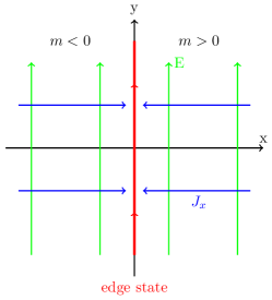
Figure 1: The setup of the system. As explained in the main text of Sec.1, the fermion mass changes sign at $x=0$, and therefore the Chern number is $1/2$ at the $x>0$ region and $-1/2$ at the $x<0$ region. In the presence of an uniform electric field in the y-direction (green arrows), the Hall currents (blue arrows) in the two regions flow in opposite directions. Therefore, there will be charge accumulation at the edge. The red arrows denote the edge current.

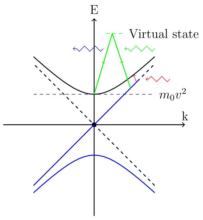
(a)

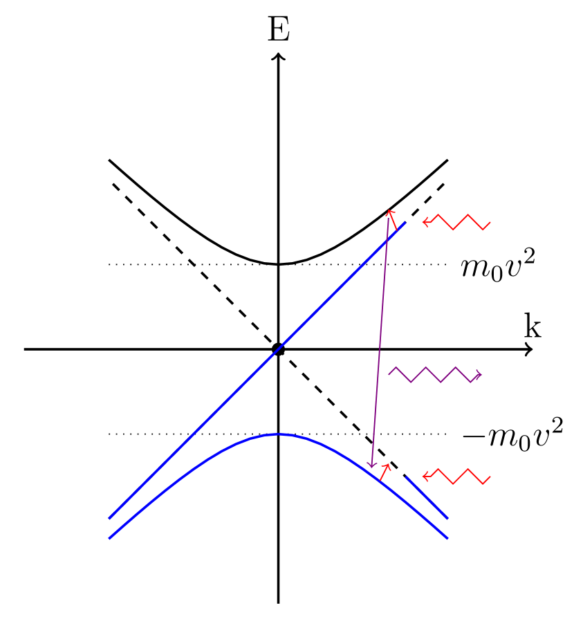
(b)

Figure 2: The energy spectra for electron systems and the edge-to-bulk transition processes. The blue and black lines describe the unoccupied and occupied states, respectively. Zigzag lines represent ingoing or outgoing photons. (a) A semi-infinite electron system with one edge or domain wall. There is only one chiral mode, whose occupied states are depicted by the straight blue line. The red arrow depicts the leading-order excitation process, which absorbs one photon. The green arrows are related to the second-order relaxation process, which includes an absorption of a low-energy photon (green zigzag line) and an emission of a high-energy photon (blue zigzag line). (b) The schematic diagram of transitions in a finite-sized system with two edges. The two straight blue lines represent the occupied edge states. The red and purple arrows denote the absorption and emission processes, while the red and purple zigzag lines denote the ingoing and outgoing photons, respectively.

In the following, we construct the eigenstates (wave functions) of the non-interacting theory, i.e. $e=0$ in Eq.1 and from now on we always assume $0<m_{0}<<M$, i.e. the vacuum gap is much bigger than the massive Chern insulator gap. Equivalently, the theory can be described in terms of the Hamiltonian

$$H=-vi\partial_{x}\sigma_{x}-vi\partial_{y}\sigma_{y}+m(x)v^{2}\sigma_{z}.$$ (5)

The spinor $\psi$ has two components, thus the equation $H\psi=E\psi$ includes two coupled first-order differential equations.

Since there is no $y$-dependence in the Hamiltonian (5), the momentum along the $y$-direction is conserved, such that the partial derivative $-i\partial_{y}$ can be replaced by a constant $p_{2}$. Therefore, we assume $\psi(t,x,y)=\Xi(x)e^{-iEt+ip_{2}y}$, and then the spinor $\Xi=(\xi_{1},\xi_{2})^{T}$ satisfies the following equation for $x>0$

$$\begin{pmatrix}m_{0}v^{2}&-vi\partial_{x}-ivp_{2}\\ -vi\partial_{x}+ivp_{2}&-m_{0}v^{2}\end{pmatrix}\begin{pmatrix}\xi_{1}\\ \xi_{2}\end{pmatrix}=E\begin{pmatrix}\xi_{1}\\ \xi_{2}\end{pmatrix}.$$ (6)

In order to solve the above differential equations, we transform them into a second order differential equation for component $\xi_{1}$:

$$\partial_{x}^{2}\xi_{1}+[(E/v)^{2}-(m_{0}v)^{2}-p_{2}^{2}]\xi_{1}=0.$$ (7)

The other component $\xi_{2}$ can be expressed by $\xi_{1}$ as

$$\xi_{2}=\frac{(-iv\partial_{x}+ivp_{2})\xi_{1}}{E+(m_{0}v)^{2}}.$$ (8)

There is one edge state (bound state) localized around $x=0$, which is given by

$$\Xi^{(e)}(x)=\sqrt{m_{0}v}\begin{pmatrix}1\\ i\end{pmatrix}e^{-m_{0}vx}$$ (9)

with the energy $E=vp_{2}$. The bulk states (continuous states) are

$$\Xi_{p_{1},p_{2}}(x)=a\begin{pmatrix}1\\ \frac{vp_{1}+ivp_{2}}{E+m_{0}v^{2}}\end{pmatrix}e^{ip_{1}x}+b\begin{pmatrix}1\\ \frac{-vp_{1}+ivp_{2}}{E+m_{0}v^{2}}\end{pmatrix}e^{-ip_{1}x}$$ (10)

The coefficients $a$ and $b$ are normalization constants, and can be found by the normalization condition $\int\Xi_{p_{1},p_{2}}^{\dagger}(x)\Xi_{p^{\prime}_{1},p_{2}}(x)dx=\delta(p_{1}-p^{\prime}_{1})$. The result is given by

$$a=-\frac{E+m_{0}v^{2}-vp_{2}-ivp_{1}}{2\sqrt{2\pi E(E-vp_{2})}}\qquad\text{and}\qquad b=\frac{E+m_{0}v^{2}-vp_{2}+ivp_{1}}{2\sqrt{2\pi E(E-vp_{2})}}$$ (11)

III Interaction with a planar photon (QED₃)

In this section, we consider a 2+1 D Dirac fermion interacting with a 2+1 D photon. It is a toy model for the interaction between the electrons in a two-dimensional plane and the photons. While electrons can be confined to the two-dimensional plane in the laboratory, photons only exist in three-dimensional space. 3+1 D photons will be considered in the next section. It is instructive, however, to start with QED₃, i.e. the case where both electrons and photons live in the two-dimensional plane. Furthermore, we take into account that the Fermi velocity for electrons in solids ís much smaller than the speed of light i.e. $v<<c$.

The action is given by

$$S_{2}=S_{1}+\frac{1}{2}\int d^{3}z\Big{(}\dot{A_{0}}^{2}-c^{2}\sum_{i=1,2}(\partial_{i}A_{0})^{2}\Big{)}$$ (12)

where $S_{1}$ is given in Eq.1 and $A_{0}$ is the temporal component of the photon field. The spatial components $A_{1}$ and $A_{2}$ are neglected in the following, because of the small Fermi velocity Araki_2010 . The interaction term $e\psi^{\dagger}\psi A_{0}$ is responsible for the transitions from edge states to bulk states, and the coupling strength $e$ is the electron charge in 2+1 D, which has the dimension 1/2, and scales as $E^{1/2}$, where $E$ is energy.

Since the speed of light is much bigger than the Fermi velocity, $c>>v$, a transition process from an edge state to a upper-band bulk state with lower energy cannot happen at the first order, i.e. a high-energy edge state cannot decay into a low-energy upper-band bulk state, by emitting only one photon. On the contrary, an electron at edge state can absorb one photon and be excited into a bulk state with a higher energy (see the red arrow in Fig. 2(a) ). Due to the photon absorption, a finite (nonzero) temperature is necessary for such a process to occur. This is the main focus of this section. The leading order contribution to a real relaxation process (from a high energy initial state to a low energy final state) comes from the second order, which is similar to Compton scattering in quantum electrodynamics. It is depicted by the green arrows, in Fig. 2(a). The corresponding process can be described by the effective Hamiltonian $H_{eff}=\lambda\psi^{\dagger}\psi A_{0}^{2}$, where $\lambda=e^{2}/E^{*}$, and $E^{*}$ is a characteristic energy related to the virtual intermediate state (shown by the green dashed line in Fig.2(a)). However, it is a high-order process suppressed by the higher power of the coupling constant.

The time evolution of the density matrix $\rho$ is governed by the equation $\dot{\rho}=-i[H_{I},\rho]$, where $H_{I}=e\psi^{\dagger}\psi A_{0}$ is the interaction term of the Hamiltonian in the interaction picture. In Born approximation, the total density matrix $\rho$ is assumed to be factorized into $\rho=\rho_{S}\otimes\rho_{B}$, where $\rho_{S}$ is the density matrix of the electron system and $\rho_{B}$ is the density matrix of the bath or the bosons (photons). Tracing out the degree of freedom of the bath environment, the evolution of the electron system $\rho_{S}=Tr_{B}(\rho)$ can be formulated by book_Breuer

$$\dot{\rho}_{S}=-\int_{0}^{t}dsTr_{B}[H_{I}(t),[H_{I}(s),\rho(s)]]$$ (13)

$$=-\int_{0}^{\infty}dsTr_{B}[H_{I}(t),[H_{I}(t-s),\rho_{S}(t)\otimes\rho_{B}]].$$ (14)

in which the Markov approximation has been applied in the second equation. We only consider the first order contribution in perturbation theory, and assume that multi-particle excitations are suppressed. Taking the average value on the edge state $|k_{e}>$ (the state means adding one edge state to the Fermi sea $|k_{e}>\otimes|FS>$, but the Fermi sea $|FS>$ will not be mentioned below for simplicity), one obtains the time evolution of the occupation probability of the state $|k_{e}>$, which is given by $<k_{e}|\dot{\rho}_{S}|k_{e}>=-I_{1}+I_{2}+h.c.$ with

$$I_{1}=\int_{0}^{\infty}dsTr_{B}<k_{e}|H_{I}(t)H_{I}(t-s)\rho_{S}(t)\otimes\rho_{B}|k_{e}>,$$ (15)

and

$$I_{2}=\int_{0}^{\infty}dsTr_{B}<k_{e}|H_{I}(t)\rho_{S}(t)\otimes\rho_{B}H_{I}(t-s)|k_{e}>.$$ (16)

$I_{1}$ is the rate of the electron leaving from the edge state $|k_{e}>$ to bulk states, while $I_{2}$ is the rate of the electron coming to the state $|k_{e}>$. These rates are related to the photon number distribution law. The rate or the speed of the latter process (photon emission) is higher than the former one (photon absorption). Furthermore, at exact zero temperature, the photon absorption process can not happen at all, but the emission process can still happen.

In the present work, we consider nonzero temperature $T$ only in the photon sector of the theory, such that the related thermal energy is much smaller than the bulk gap $k_{B}T<<2m_{0}v^{2}$. Therefore, if the chemical potential of the edge state $\mu<<m_{0}v^{2}$, the temperature is not large enough to efficiently supply a photon for the excitation of edge state into a bulk one. On the other hand, if edge’s $\mu>m_{0}v^{2}$ and we consider the edge state with momentum $k_{e}$ such that $v\sqrt{k_{e}^{2}+(m_{0}v)^{2}}-vk_{e}\sim k_{B}T$, the excitation process to the bulk can indeed happen, even at small temperature of the photon bath $k_{B}T<<2m_{0}v^{2}$. We consider this process as a main contribution to the relaxation of the edge states, neglecting other possible processes. As was mentioned above, the ”Compton-like” relaxation depicted by the green arrows in Fig. 2(a) is suppressed by the second power of the interaction constant. Furthermore, we neglect the backward relaxation $I_{2}$.

In order to devise the arguments in favor of this approximation, we consider a finite-width system, e.g. a ribbon, with two edges (domain-walls). Fig.2(b) shows the energy occupation state and transition processes for the two-edge system. There are two edges states now denoted by the straight dashed lines and straight blue lines in Fig.2(b). If the electric field is parallel to the edges, the Hall current is perpendicular to the edges and drives the charge from one edge to another. Therefore, the chemical potential of one edge will decrease (depletion process), and the chemical potential of the other edge will increase (accumulation process). Because the two edges are far from each other, direct transition from one edge to another is difficult, if not completely impossible. Direct calculation of the transition rate from edge to edge gives the estimation of the order of ${\rm exp}(-m_{0}L_{x})$, with $L_{x}$ the distance between the two edges, i.e. the width of the ribbon, and $m_{0}$ is the fermion mass in the bulk. In contrast, the transition rate from edge to bulk is of the order of $1/\sqrt{m_{0}L_{x}}$. If $L_{x}$ is large enough ($m_{0}L_{x}>>1$), both rates are small, but the former is much smaller than the latter, thus we neglect the direct transitions from one edge to another. The $I_{1}$ relaxation processes happen in both edges, leading to the appearance of holes in the lower band in the bulk. It opens the possibility for the direct transitions from upper to lower band in the bulk via the photon emission depicted by the purple arrows in Fig. 2(b). These processes are of the order of $1$. It means that they are much faster than all edge-bulk transitions and they keep the upper band of the bulk almost empty, thus suppressing the inverse bulk-to-edge transitions denoted by $I_{2}$. Thus we conclude that the time of the whole edge-to-bulk relaxation is determined by the comparatively slower process $I_{1}$ showed by red arrows in Fig.2(b).

In order to further calculate $I_{1}$, we neglect the off-diagonal elements of the density matrix and insert a complete set of states between the two $H_{I}$ operators (many-particle excitations are neglected). Then the rate $I_{1}$ can be reformulated into

$$I_{1} = \int_{0}^{\infty}dsTr_{B}<k_{e}|H_{I}(t)|\mathbf{p}>\frac{d^{2}p}{(2\pi)^{2}}<\mathbf{p}|H_{I}(t-s)\rho_{S}(t)\otimes\rho_{B}|k_{e}>,$$ (17)

$$= e^{2}\int\frac{d^{2}p}{(2\pi)^{2}}W_{k_{e}}(\mathbf{p})\,r(k_{e},t),$$

where $|k_{e}>$ is the edge state with momentum $k_{e}$, $|\mathbf{p}>$ is the bulk state with momentum $\mathbf{p}=(p_{1},p_{2})$, and the function $r(k_{e},t)$ is defined by $<k^{\prime}_{e}|\rho_{S}(t)|k_{e}>=r(k_{e},t)\delta(k^{\prime}_{e}-k_{e})$. The quantity

$$W_{k_{e}}(\mathbf{p}) = \int_{0}^{+\infty}ds\int_{0}^{+\infty}dx\int_{0}^{+\infty}dx^{\prime}\int\int dydy^{\prime}e^{iEs}$$ (18)

$$f_{\mathbf{p}}(x)f^{*}_{\mathbf{p}}(x^{\prime})e^{i(p_{2}-k_{e})(y-y^{\prime})}G(s,x-x^{\prime},y-y^{\prime})$$

where $f_{\mathbf{p}}(x)=\Xi^{(e)\dagger}\Xi_{\mathbf{p}}(x)$ is the inner product of the spinors, and $G(s,x-x^{\prime},y-y^{\prime})=Tr_{B}[\rho_{B}\phi_{-}(s,x-x^{\prime},y-y^{\prime})\phi_{+}(0,0,0)]$ is the correlation function of the photon field. The field $A_{0}$ is decomposed into $A_{0}=\phi_{+}+\phi_{-}$, with $\phi_{+}$ the positive frequency component including the annihilation operators and $\phi_{-}$ the negative frequency component including the creation operators. The other combination $Tr_{B}[\rho_{B}\phi_{+}\phi_{-}]$ is neglected by virtue of the rotating wave approximation book_Breuer .

The photon correlation function $G$ can be calculated by mode expansion, and the result (in Gaussian units) is

$$G(t,x,y)=\int\frac{c^{2}d^{2}q}{(2\pi)^{2}2\omega_{q}}n_{B}(\omega_{q})e^{i\omega_{q}t-iq\cdot r},$$ (19)

where $n_{B}(\omega)=1/(e^{\beta\omega}-1)$ is the Bose-Einstein distribution function for the photon bath, $\beta=1/({\rm k_{B}}T)$, $\omega_{q}=c\sqrt{q_{1}^{2}+q_{2}^{2}}$, $q=(q_{1},q_{2})$ and $r=(x,y)$. Therefore, we found

$$W_{k_{e}}(\mathbf{p})=\int\frac{d^{2}q}{(2\pi)^{2}\omega_{q}}|F_{\mathbf{p},q_{1}}|^{2}L_{y}\delta(p_{2}-k_{e}+q_{2})\delta(E(k_{e})-E_{\mathbf{p}}+\omega_{q})n_{B}(\omega_{q}),$$ (20)

where $F_{\mathbf{p},q_{1}}=\int_{0}^{+\infty}f_{\mathbf{p}}(x)e^{iq_{1}x}dx$ and

$$|F_{\mathbf{p},q_{1}}|^{2}=\frac{v^{2}p_{1}q_{1}}{\pi E_{\mathbf{p}}(E_{\mathbf{p}}-vp_{2})}\Big{[}\frac{m_{0}v}{(q_{1}-p_{1})^{2}+(m_{0}v)^{2}}-\frac{m_{0}v}{(q_{1}+p_{1})^{2}+(m_{0}v)^{2}}\Big{]}.$$ (21)

For simplicity, the function $\frac{m_{0}v}{q^{2}+(m_{0}v)^{2}}$ is replaced by $\pi\delta(q)$, and then function $W_{k_{e}}(\mathbf{p})$ can be evaluated as

$$W_{k_{e}}(\mathbf{p})=L_{y}\delta(E(k_{e})-E_{\mathbf{p}}+\omega_{p_{1},k_{e}-p_{2}})\frac{v^{2}p_{1}^{2}n_{B}(\omega_{p_{1},k_{e}-p_{2}})}{\pi E_{\mathbf{p}}(E_{\mathbf{p}}-vp_{2})\omega_{p_{1},k_{e}-p_{2}}}.$$ (22)

Therefore, the transition rate of the edge state $|k_{e}>$ to the bulk states is given by

$$\Gamma(k_{e})=e^{2}\int W_{k_{e}}(\mathbf{p})\frac{d^{2}p}{(2\pi)^{2}}.$$ (23)

Its integrand includes the delta function $\delta(E(k_{e})-E_{\mathbf{p}}+\omega_{p_{1},k_{e}-k})$, with $E_{p_{1},p_{2}}=v\sqrt{p_{1}^{2}+p_{2}^{2}+(m_{0}v)^{2}}$ and $\omega_{p_{1},p_{2}}=c\sqrt{p_{1}^{2}+p_{2}^{2}}$. If the Fermi velocity $v$ is much smaller than the speed of light $c$, i.e. $v/c\sim 1/100$, then it is safe and convenient to replace $E_{\mathbf{p}}$ in the integrand by $E_{0,k_{e}}$. After integrations, we obtain the result of the transition rate per unit length $\Gamma_{1}(k_{e})=\Gamma(k_{e})/L_{y}$ as follows

$$\Gamma_{1}(k_{e})=\frac{e^{2}v^{2}\Delta E}{\pi c^{2}E_{0,k_{e}}}n_{B}(\Delta E),$$ (24)

with $\Delta E=E_{0,k_{e}}-E(k_{e})$. When $k_{e}\rightarrow+\infty$, $\Delta E\rightarrow 0^{+}$ and $\Gamma_{1}(k_{e})$ goes to zero as $\sim{\rm k_{B}}T/k_{e}$. The $k_{e}$-dependence of function $\Gamma_{1}(k_{e})$ is shown by curve 1 in Fig.3(a).

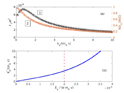
Figure 3: (a)The black curve (marked by label 1) shows the momentum dependence of the excitation rate $\Gamma_{1}(k_{e})/e^{2}$ of the edge state $|k_{e}>$. It is computed according to Eq.24, with $v/c=0.01$. The horizontal axis is $k_{e}/(m_{0}v)$. The black curve (marked by label 2) is the the distribution function $R(k_{e})/R(0)$ in the saturation state, i.e. Eq.26, with the electric field $E_{y}=2\times 10^{-5}em_{0}v$ related to the red dotted line in Fig.(b). (b) The saturation momentum $K_{e}^{*}$ obtained from Eq. 25 as a function of electric filed $E_{y}$, in the step-function approximation for the edge-state occupancy.

Now let us analyze the consequences of such an excitation process, and consider the evolution of the occupancy of the edge states. Suppose at time $t=0$, the chemical potential of the whole system is at $\mu=0$ (Fig.2(a)), and one turns on the electric field in the y-direction $E_{y}$. On the one hand, because of the electric field, there is a constant rate of electrons flowing toward the edge and accumulating there. On the other hand, the accumulated electrons at the edge are excited via thermal fluctuations and transferred to the bulk. If we assume that at a time $t$ the edge states are occupied up to the momentum $K_{e}(t)$ , what is its behavior at the later times $t\rightarrow\infty$? Is it possible for the system to reach a saturation? A ”saturation” means a balance between the inflow current towards the edge and the excitation process depleting the edge. The excitation rate from the edge to the bulk $\int_{0}^{K_{e}}\Gamma_{1}(k_{e})dk_{e}$ is small in the beginning (for small $t$) because $K_{e}$ is small i.e. $K_{e}(t)\sim 0$. Therefore the accumulation process is stronger than the depletion, and $K_{e}$ starts to increase. When $K_{e}$ increases, the rate of depletion also increases. If the depletion rate coincides with the accumulation rate, the process reaches equilibrium, and $K_{e}$ saturates. In order to calculate the saturation momentum $K_{e}^{*}$, we equate the two rates (number of particles per unit time and per unit length)

$$\int_{0}^{K_{e}^{*}}\Gamma_{1}(k_{e})dk_{e}=\sigma_{H}E_{y}/e.$$ (25)

Finite values of $K_{e}^{*}$ can be found, as a function of $E_{y}$, which is shown in Fig.3 (b). Asymptotically, $K_{e}^{*}(E_{y})$ scales as $\sim{\rm exp}(E_{y}/em_{0}v)$, for large $E_{y}$.

Above, we assumed the distribution function on the edge $r(k_{e})$ to be a step function: $r(k_{e})=1$ when $k_{e}<K_{e}$ and $r(k_{e})=0$ when $k_{e}>K_{e}$. Such an assumption is simple, but is not entirely realistic. In order to approach reality, we lift such an assumption, and allow the distribution function $r(k_{e},t)$ to take any value between zero and one. We are going to find such a distribution function at the saturation ($t\rightarrow+\infty$). Suppose $\Delta t$ is a very short time interval and $k^{\prime}_{e}=k_{e}+E\Delta t$, and then we have $r(k^{\prime}_{e},t+\Delta t)=r(k_{e},t)(1-\Gamma_{1}(k_{e})\Delta t)$. It means that the momentum of the edge-state fermions is changed by the electric field $E_{y}$ during the time interval, and in the meantime, the fermions leave the edge (via excitation process) at the rate $\Gamma_{1}$. In the stationary state, $r(k_{e},t+\Delta t)=r(k_{e},t)$, which doesn’t depend on time, and can be denoted by the function $R(k_{e})$. Therefore, we obtain $R^{\prime}(k_{e})E_{y}=-\Gamma_{1}(k_{e})R(k_{e})$, from which we find the function $R(k_{e})$ as the final distribution along the edge:

$$R(k_{e})/R(0)={\rm exp}\Big{(}-\int_{0}^{k_{e}}\Gamma_{1}(k^{\prime})dk^{\prime}/E_{y}\Big{)},$$ (26)

which is shown by curve 2 in Fig.3 (a).

IV Interaction with 3+1 D photons

In this section we consider a realistic model, where the 2+1 D electrons interact with 3+1 D photons. The corresponding action is given by

$$S_{3}=S_{1}+\frac{1}{2}\int d^{4}x\Big{(}\dot{A_{0}}^{2}-c^{2}\sum_{i=1}^{3}(\partial_{i}A_{0})^{2}\Big{)},$$ (27)

where $d^{4}x=dt\,dx\,dy\,dz$. The 2+1 D electron system is located on the $z=0$ plane.

The deduction in the previous section about the evolution of the density matrix and the transition rate can be repeated straightforwardly. However, the photon correlation function $G$ in Eq.19 has to be modified, because of the different dimensionality. As for 3+1 D photon, the corresponding correlation function $\mathcal{G}(s,x-x^{\prime},y-y^{\prime})$ is defined as

$$\mathcal{G}(s,x-x^{\prime},y-y^{\prime})=Tr_{B}[\rho_{B}\phi_{-}(s,x,y,0)\phi_{+}(0,x^{\prime},y^{\prime},0)],$$ (28)

where the $z$ component of the spatial coordinates is fixed to be 0, because the photons interact with the fermions only at the $z=0$ plane. The result of $\mathcal{G}$ can be obtained by mode expansion

$$\mathcal{G}(t,x,y)=\int\frac{d^{3}q}{(2\pi)^{3}2\omega_{q}}n_{B}(\omega_{q})e^{i\omega_{q}t-iq_{1}x_{1}-iq_{2}x_{2}},$$ (29)

where $q=(q_{1},q_{2},q_{3})$, and $\omega_{q}=c\sqrt{q_{1}^{2}+q_{2}^{2}+q_{3}^{2}}$. Corresponding to Eq.22, the function $W$ for 3+1 D photon will be given by

$$W_{k_{e}}(\mathbf{p})=L_{y}\int\frac{dq_{3}}{2\pi}\delta(E(k_{e})-E_{\mathbf{p}}+\omega_{p_{1},k_{e}-p_{2},q_{3}})\frac{v^{2}p_{1}^{2}n_{B}(\omega_{p_{1},k_{e}-p_{2},q_{3}})}{\pi E_{\mathbf{p}}(E_{\mathbf{p}}-vp_{2})\omega_{p_{1},k_{e}-p_{2},q_{3}}}.$$ (30)

From the function $W_{k_{e}}(\mathbf{p})$, we obtained the transition rate of the edge state $k_{e}$ to the bulk

$$\Gamma_{1}(k_{e})=(e^{2}/L_{y})\int W_{k_{e}}(\mathbf{p})\,d^{2}p/(2\pi)^{2},$$

and its result is given by

$$\Gamma_{1}(k_{e})=\frac{4\alpha v^{2}\Delta E^{2}n_{B}(\Delta E)}{3c^{2}E_{0,k_{e}}}.$$ (31)

with $\alpha=e^{2}/c$ and $\Delta E=E_{0,k_{e}}-vk_{e}$. Then as in the previous section, one can figure out the charge accumulation at the edge and the stationary distribution law of the edge electrons in momentum space, which is shown in Fig.4.

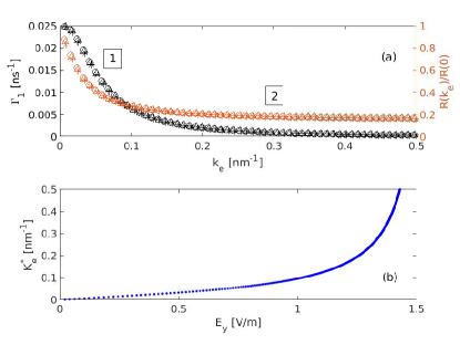
Figure 4: (a)The black curve (marked by label 1) is the excitation rate $\Gamma_{1}(k_{e})$, as a function of momentum $k_{e}$, Eq.31. ns is nanosecond. The parameters are given as follows: the bulk gap $\Delta=2m_{0}v^{2}=0.1{\rm eV}$, Fermi velocity $v=0.01c$ and the temperature ${\rm k_{B}}T=\Delta/4$. The red curve (marked by label 2) is the the occupation function $R(k_{e})/R(0)$ in the saturation state, with $E_{y}=0.75\,V/m$. It is obtained from Eq.26, with the $\Gamma_{1}(k_{e})$ function given by Eq.31. (b) The saturation momentum $K_{e}^{*}$ in the step-function assumption for the edge occupation, v.s. electric filed $E_{y}$. One observes that there is a critical electric field, around $1.5\,V/m$, above which the value of $K_{e}^{*}$ diverges.

From Eq.31, one notices that when $k_{e}\rightarrow+\infty$, $\Gamma_{1}(k_{e})$ goes to zero as $1/k^{2}_{e}$, implying that $\int^{+\infty}\Gamma_{1}(k_{e})dk_{e}$ is a finite number. As in the previous section, the saturation momentum $K_{e}^{*}$ can be specified by Eq. 25 according to the assumption of step-function edge-state distribution. However, if the electric field $E_{y}$ is larger than the critical field $E_{y}^{(c)}=\int_{0}^{+\infty}\Gamma_{1}(k_{e})dk_{e}/(\sigma_{H}L_{y})$, then the saturation momentum $K_{e}^{*}$ will be infinite. It means all the edge states will be occupied, if the electric field is strong enough. This ”electron avalanche” phenomenon is due to our low-energy effective model which is not regularized by the high energy part of the dispersion relation as it always appears in real materials. If $K_{e}^{*}$ is very large, the higher momentum part of the band structure should be taken into account, and the dispersion curve will bend, which prevents $K_{e}^{*}$ from going to infinity.

We will now discuss the realization of such an effect in the laboratory, and estimate the order of magnitudes for the physical quantities. In the last section, we considered half infinite planar systems, and infinitely long ribbon-shaped systems. The former one has only one boundary, while the latter one has two boundaries. However, both of them are hard to realize in experiment. Instead of these infinite-sized systems, we consider a cylinder with finite length or an annulus as more realistic examples. Both of them are finite sized and have one hole and two edges. If the magnetic field going through the hollow part of this kind of a system varies with time, the electric field parallel to the edges appears automatically. Due to this electric field, the Hall current is perpendicular to the edges and drives the charge from one edge to another. Therefore, the chemical potential of one edge will decrease (depletion process), and the chemical potential of the other edge will increase (accumulation process), exactly as shown in Fig.2(b).

At last, we estimate the orders of the main quantities, such as the transition rate $\Gamma_{1}(k_{e})$ and the critical electric field $E_{y}^{(c)}$. In Fig. 4 we show how the edge-to-bulk transition rate changes with the wave vector of the edge state $k_{e}$. One can see that the transition rate is of the order of ns^-1 (nanosecond) and it decreases with the increase of the wave vector $k_{e}$. For a massive Chern insulator with gap $\Delta=0.1{\rm eV}$, at temperature given by ${\rm k_{B}}T=\Delta/4$, i.e. $T\sim 250\,{\rm K}$, the rate at which edge-state electrons transition into the bulk (per unit length of the edge) is about $3\times 10^{14}\,m^{-1}s^{-1}$. If the size of a sample is $1\mu m$, the rate is $3\times 10^{8}\,s^{-1}$. It means the life time of an edge state will be about 3 $ns$. The critical electric field is about 1.5 V/m, which does not depend on the the size of the sample.

V Conclusion and Outlook

In the present work, we revisited the Callan-Harvey mechanism in Jackiw-Rebbi model with a space-dependent domain wall mass. Due to the parity anomaly, the electric field, which is parallel to the domain wall (the edge), drives the electrons to the edge. As the electrons accumulate along the edge, they starts to transfer into the bulk states via thermal fluctuation. We studied the time evolution of the surplus charge at the edge in the Lindblad formalism, and the transition rate from the edge to the bulk was calculated. In such a transition process, photon absorption is necessary. Therefore, at zero temperature, the transition process does not occur in our electron-photon interaction model, and the charge accumulation at the edge will be boundless. At finite (non-zero) temperature, we studied the stationary state at late times $t\rightarrow+\infty$. In the planar photon (QED₃) case, the stationary state can be obtained for arbitrary electric field. In the 3+1 D photon case, there is a critical electric field strength $E^{(c)}$, below which the stationary state exists, but above which the stationary state does not exist and the charge accumulation will be boundless.

Our present study investigated the effects of electron-photon interaction on the edge states, and improved the physical picture of Callan-Harvey mechanism with dissipation processes. It has not only scholar interest from quantum field theories, but also might have potential applications in the condensed matter (optical relaxation in topological materials) and potential applications in engineering. For example, the optical processes depicted in Fig.2(b) might make such a system into a new light source: in the presence of an electric field, the system absorbs two low-energy photons from the thermal bath (the environment), and then emits one high-energy photon, with the energy $\sim\Delta$ the band gap. Furthermore, if one replaces the (low-energy) thermal photons (the red zigzag lines in Fig.2(b)) by incident photons with the same energy, then the incident photons trigger the relaxation (the purple zigzag line in Fig.2(b)), and vice versa.

There are also several directions for the future. In the present work, we considered the Dirac mass term, which is a constant within a bulk region. A natural generalization is to study the momentum dependent mass, as in the Bernevig–Hughes–Zhang (BHZ) model. Besides, electron-phonon interactions should be taken into account in the condensed matter systems, and the heat dissipation effect can be studied.

- (1) S.L. Adler, ”Axial vector vertex in spinor electrodynamics”. Phys. Rev. 177, 2426 (1969).
- (2) J.S. Bell and R. Jackiw, ”A PCAC Puzzle: in the sigma model”. Nuovo Cim. A 51, 47 (1969).
- (3) D. Kharzeev, ”The Chiral Magnetic Effect and anomaly-induced transport”. Progress in Particle and Nuclear Physics 75, 133 (2014). arXiv:1312.3348
- (4) F. D. M. Haldane, Model for a Quantum Hall Effect without Landau Levels: Condensed-Matter Realization of the ”Parity Anomaly”. Phys. Rev. Lett. 61, 2015 (1988).
- (5) C.X. Liu, S.C. Zhang, and X.L. Qi, ”The Quantum Anomalous Hall Effect: Theory and Experiment”. Annual Review of Condensed Matter Physics 7, 301 (2016).
- (6) C. G. Callan and J. A. Harvey, ”Anomalies and fermion zero modes on strings and domain walls”. Nucl. Phys. B 250, 427 (1985).
- (7) R. B. Laughlin, ”Quantized Hall conductivity in two dimensions”, Phys. Rev. B 23, 5632(R) (1981).
- (8) J. Böttcher, C. Tutschku, L.W. Molenkamp and E.M.Hankiewicz, ”Survival of the Quantum Anomalous Hall Effect in Orbital Magnetic Fields as a Consequence of the Parity Anomaly”, Phys. Rev. Lett. 123, 226602 (2019); J. Böttcher, C. Tutschku and E.M.Hankiewicz, ”Fate of quantum anomalous Hall effect in the presence of external magnetic fields and particle-hole asymmetry”, Phys. Rev. B 101, 195433 (2020).
- (9) A. J. Niemi and G. W. Semenoff, ”Axial-Anomaly-Induced Fermion Fractionization and Effective Gauge-Theory Actions in Odd-Dimensional Space-Times”. Phys. Rev. Lett. 51, 2077 (1983).
- (10) S. Chandrasekharan, ”Anomaly cancellation in 2+1 dimensions in the presence of a domain wall mass”, Phys. Rev. D 49, 1980 (1994).
- (11) D. Tong, ”Lectures on String Theory”, p 110.
- (12) B. V. Pashinsky, M. Goldstein, and I. S. Burmistrov, ”Finite frequency backscattering current noise at a helical edge”, Phys. Rev. B 102, 125309 (2020).
- (13) O. Heinonen, ”Deviations from perfect integer quantum Hall effect”, Phys. Rev. B 46, 1901(R) (1992).
- (14) F. Lafont, R. Ribeiro-Palau, et al, ”Anomalous dissipation mechanism and Hall quantization limit in polycrystalline graphene grown by chemical vapor deposition”, Phys. Rev. B 90, 115422 (2014).
- (15) G. W. Semenoff, ”Condensed-Matter Simulation of a Three-Dimensional Anomaly,” Phys. Rev. Lett. 53, 2449 (1984).
- (16) C. Xiong, ”QCD flux tubes and anomaly inflow”, Phys. Rev. D 88, 025042 (2013).
- (17) K. Fukushima and S. Imaki, ”Anomaly inflow on QCD axial domain-walls and vortices”, Phys. Rev. D 97, 114003 (2018).
- (18) C. Tutschku, J. Böttcher, R. Meyer, and E. M. Hankiewicz, ”Momentum-dependent mass and AC Hall conductivity of quantum anomalous Hall insulators and their relation to the parity anomaly”, Phys. Rev. Research 2, 033193 (2020).
- (19) P.V. Buividovich and M.V. Ulybyshev, ”Numerical study of chiral plasma instability within the classical statistical field theory approach”, Phys. Rev. D 94, 025009 (2016).
- (20) R. Jackiw and C. Rebbi, ”Solitons with fermion number ”, Phys. Rev. D 13, 3398 (1976).
- (21) Y. Araki and T. Hatsuda, ”Chiral gap and collective excitations in monolayer graphene from strong coupling expansion of lattice gauge theory”, Phys. Rev. B 82, 121403(R) (2010).
- (22) H. Breuer, The Theory of Open Quantum Systems, 2007.