Dickman multiple polylogarithms
and the Lindemann–Furry letters
David Broadhurst and Stephan Ohlmeyer
30 April 2023

Abstract: The Dickman function $\rho(u)$ gives the asymptotic probability that a large integer $N$ has no prime divisor exceeding $N^{1/u}$. We expand it in terms of rapidly computable multiple polylogarithms, as defined by Goncharov and intensively used for evaluations of Feynman integrals in quantum field theory. In parallel, we solve Buchstab’s differential-delay equation, which concerns large integers $N$ divisible by no prime less than $N^{1/u}$. Discussion of the latter problem occurred in letters to the journal Nature during the second world war, from the physicists Frederick Lindemann and Wendell Furry. We recount how Furry evaluated a dilogarithm in reply to a puzzle resulting from Mertens’ third theorem, raised by Lindemann. We refine Furry’s analysis to include multiple polylogarithms of weights up to 200.

1 Introduction

In 1930, Karl Dickman considered smooth numbers, all of whose prime divisors are smaller than a certain magnitude [30]. In 1937, Aleksandr Buchstab considered rough numbers, none of whose prime divisors are smaller than such a magnitude [19]. These cognate problems received further attention after the second world war, notably from Nicolaas de Bruijn [15, 16, 17]. During that war, Lindemann and Furry addressed the problem of rough numbers, which clearly include primes.

Replying [38] to a letter [52] by Lindemann, Number of primes and probability considerations, Furry deftly computed the asymptotic density of numbers of size $N$ divisible by no prime $p\leq N^{1/4}$. These comprise primes, semiprimes and integers with three prime divisors, all of which are greater than $N^{1/4}$. From this analysis, he obtained an approximation to $e^{-\gamma}$ with an absolute error less than $1.25\times 10^{-6}$, where the Euler–Mascheroni constant $\gamma$ emerges from a combination of Mertens’ third theorem with probabilistic reasoning, as suggested by Lindemann. In achieving this, Furry dealt with dilogarithms [50], in advance of their application to quantum field theory by Schwinger [70], and with a Mertens product, in advance of Buchstab’s later work [20] in 1951, which cites Brun’s use of the sieve of Eratosthenes [18].

The Dickman problem [30] for smooth [61] numbers was considered by many post-war authors, both before [25, 68] and after [6, 22, 44, 45, 48] de Bruijn [16], since issues of smoothness and semi-smoothness [4] are of importance in situations where one hopes to make progress in factorizing large composite numbers [12].

In this article, we explain the context of Furry’s letter on the Buchstab problem [19], written when he was working on radar in USA, and Lindemann’s letter, written when he was Churchill’s scientific advisor, much preoccupied with the war effort in UK. Moreover we develop Furry’s analysis to include multiple polylogarithms of weights up to 200, using techniques devised for calculations in quantum field theory, where a pressing need to understand phenomena at the Large Hadron Collider (LHC) has resulted in computational progress, albeit for integrals with lesser weights [62, 72] .

For $u>1$ the Dickman function $\rho(u)$ satisfies the differential-delay equation [16]

$$u\rho^{\prime}(u)=-\rho(u-1)$$ (1)

with $\rho(u)=1$ for $u\in[0,1]$. To compute it, we define multiple polylogarithms

$$M_{j,n}(y)=\sum_{n_{1}>\ldots>n_{j}>0}\;\prod_{i=1}^{j}\frac{z_{i}^{n_{i}}}{n_{i}},\quad z_{1}=\frac{y}{n},\quad z_{i}=\left(\frac{n+2-i}{n+1-i}\right)~{}\text{for}~{}i>1$$ (2)

with nested sums that converge rapidly for real $y\in[0,1]$ and integers $n>j>0$.

Theorem 1: For $y\in[0,1]$ and $n>0$,

$$\rho(n-y)=\rho(n)+\sum_{j=1}^{n-1}\rho(n-j)M_{j,n}(y).$$ (3)

This will be proved in Section 2, where it leads to a practical method for computing $\rho(u)$, for real $u\in[1,200]$, thanks to the procedure polylogmult of Pari/GP [65], which implements Henri Cohen’s efficient extension [26] of an algorithm devised by P. Akhilesh [2, 3] for Don Zagier’s multiple zeta values [7, 75].

For $u>2$, the Buchstab function $\omega(u)$ satisfies the differential-delay equation [15]

$$u\omega^{\prime}(u)=\omega(u-1)-\omega(u)$$ (4)

with $u\omega(u)=1$ for $u\in[1,2]$. Let $\sigma(u)=(u+1)\omega(u+1)$.

Theorem 2: For real $y\in[0,1]$ and $n>0$,

$$\sigma(n-y)=\sigma(n)+\sum_{j=1}^{n-1}(-1)^{j}\sigma(n-j)M_{j,n}(y).$$ (5)

Thanks to this, we shall solve the Buchstab problem in parallel with the Dickman problem, merely by changing the signs of polylogs with odd weights. For real $u>1$, the results have the form

$$\sigma(u)=1+\sum_{u>k>0}P_{k}(u),\quad\rho(u)=1+\sum_{u>k>0}(-1)^{k}P_{k}(u)$$ (6)

where the sums terminate at the largest integer less than $u$ and $P_{k}(u)$ has support only for $u>k$, where it is positive and of pure polylogarithmic weight $k$.

For $u\geq k>0$, the boundary condition $P_{k}(k)=0$ and the differential equation $uP_{k}^{\prime}(u)=P_{k-1}(u-1)$ determine $P_{k}(u)$ as an iterated integral, on the understanding that $P_{0}(u)=1$ for $u\geq 0$. Thus $P_{1}(u)=\log(u)$, for $u\geq 1$. For $u\geq 2$, we have

$$P_{2}(u)=\frac{\log^{2}(u)-\zeta_{2}}{2}+{\rm Li}_{2}\left(\frac{1}{u}\right)$$ (7)

where ${\rm Li}_{k}(z)=\sum_{n>0}z^{n}/n^{k}$, for $|z|<1$, is a classical polylogarithm [50] with ${\rm Li}_{1}(z)=-\log(1-z)$ and $z{\rm Li}_{k}^{\prime}(z)={\rm Li}_{k-1}(z)$, for $k>1$, where $\zeta_{k}={\rm Li}_{k}(1)$. To prove (7) we use the evaluation [50] ${\rm Li}_{2}(\frac{1}{2})=\frac{1}{2}\zeta_{2}-\frac{1}{2}\log^{2}(2)$, which shows that the condition $P_{2}(2)=0$ is satisfied. The differential equation $uP_{2}^{\prime}(u)=\log(u-1)$, for $u\geq 2$, is then verified as the identity $\log(u)+\log(1-1/u)=\log(u-1)$.

In 1941, Lindemann wrote a letter [52] to the editors of the journal Nature, where it was published with the title Number of primes and probability considerations. He noted the appearance of Euler’s constant $\gamma$ in Mertens’ third theorem [59]

$$\lim_{x\to\infty}\log(x)\prod_{p\leq x}\left(1-\frac{1}{p}\right)=e^{-\gamma},$$ (8)

for products over primes, and its conspicuous absence from the prime number theorem. In a reply [38] by Furry, we found an intriguing approximation

$$4e^{-\gamma}-\log(3)-\log(2)\log\left(\frac{3}{2}\right)+\frac{1}{2}\sum_{k=1}^{\infty}\frac{1}{k^{2}4^{k}}\approx 1.0000050$$ (9)

whose probabilistic origin we shall review in Section 3.

In Section 4, we study the behaviour of $P_{k}(u)$, $\sigma(u)$ and $\rho(u)$ at large $u$. Section 5 concerns the discrete situation, where we study divisibility properties of integers in finite ranges. Section 6 offers comments and conclusions.

2 Algorithms and proofs

The multiple polylogarithms $P_{k}(u)$ in the terminating series (6) are $k$-fold iterated integrals that may be evaluated as nested multiple sums [11, 69].

Theorem 3: For $u\geq k>0$,

$$P_{k}(u)=\sum_{n_{1}>\ldots>n_{k}>0}\;\prod_{i=1}^{k}\frac{z_{i}^{n_{i}}}{n_{i}},\quad z_{i}=1-\frac{1}{u-k+i}.$$ (10)

The proof is given later. Here we remark on the rate of convergence. The nested sum in (10) clearly converges, since $|z_{i}|<1$. Yet as $u$ increases, the convergence becomes slower. For $u\in[k,k+1]$, polylogmult is very efficient, giving 50 digits of $P_{10}(11)$ in less than 3 milliseconds on a 3.1 GHz machine. Yet $P_{10}(13)$ takes 34 milliseconds. If we ask Pari/GP for $P_{10}(14)$ we are politely told: sorry, polylogmult in this range is not yet implemented. To overcome this, we use Theorem 2.

2.1 Algorithms

To evaluate $\rho(u)$ and $\sigma(u)$ with $u\in[1,N]$, we begin by evaluating a triangular matrix of constants, which will be stored. Consider polynomials in $\lambda$ defined recursively by

$$S_{n}=S_{n-1}-\sum_{j=1}^{n-1}(-\lambda)^{j}S_{n-j}M_{j,n}(1)$$ (11)

for $n\in[2,N]$, with $S_{1}=1$. Then Theorem 2 gives $\sigma(n)$ as the value of $S_{n}$ at $\lambda=1$.

Algorithm 1: With symbolic $\lambda$ and numerical $M_{j,n}(1)$, perform recursion (11) and store the coefficient of $\lambda^{k}$ in $S_{n}$ as $P_{k}(n)$, for $0\leq k<n\leq N$.

With $y=1$ in the multiple polylogarithms (2) this evaluates, for example,

$$P_{1}(4) =M_{1,2}+M_{1,3}+M_{1,4},$$ (12)

$$P_{2}(4) =M_{1,2}(M_{1,3}+M_{1,4})+M_{1,3}M_{1,4}-M_{2,3}-M_{2,4},$$ (13)

$$P_{3}(4) =M_{1,2}M_{1,3}M_{1,4}-M_{2,3}M_{1,4}-M_{2,4}M_{1,2}+M_{3,4}.$$ (14)

Algorithm 2: Let $n$ be the ceiling of $u$. For $k<n$, evaluate

$$P_{k}(u)=\sum_{j=0}^{k}(-1)^{j}P_{k-j}(n-j)M_{j,n}(n-u)$$ (15)

on the understanding that the empty product gives $M_{0,n}(y)=1$ at $j=0$.

2.2 Small weights

There is a limitation to these algorithms at large $u$. The poor convergence in Theorem 3, for increasing $u-k$, has been traded for an increasing number of products in Algorithm 2, with constants from Algorithm 1 that involve products of products. This situation is well understood in the application of perturbative quantum field theory to experimental high-energy physics. The formal parameter $\lambda$ of Algorithm 1 is eventually set to $\lambda=1$, to solve the Buchstab equation, or to $\lambda=-1$, to solve the Dickman equation. It mimics the coupling constant of a perturbative expansion. Higher powers of $\lambda$ involve an increase of the maximum weight by 1. In high-energy physics, the weight may increase by 2 at the next order in $\lambda$, if the result is reducible to multiple polylogarithms [8, 31].

The Dickman argument $u$ is akin to a kinematic variable in high-energy physics, where there are situations in which polylogs become large in certain regions of phase space. In such a case, it is useful to have a leading-logarithm approximation [31]. In the Dickman problem, the leading power of a log is easily determined: $P_{k}(u)$ is asymptotic to $\log^{k}(u)/k!$. On the basis of high-precision results for $k<10$, it was conjectured in [14] that at large $u\gg k$

$$P_{k}(u)=\sum_{j=0}^{k}\frac{D_{k-j}\log^{j}(u)}{j!}+o(1),\quad\sum_{k=0}^{\infty}D_{k}z^{k}=D(z)=\frac{e^{-\gamma z}}{\Gamma(1+z)}$$ (16)

and this was later proved in [71].

This behaviour is not immediately apparent from the algorithms, which make calls to polylogmult via auxiliaries in (2) with good convergence. However, we must combine many products of such terms when $u$ is large. Consider weight 2, where we know that $P_{2}(u)=\frac{1}{2}\log^{2}(u)-\frac{1}{2}\zeta_{2}+{\rm Li}_{2}(1/u)$, for $u\geq 2$. This form is optimal at large $u$, requiring a single call to polylog with a small argument $1/u$. In contrast, our method appears profligate at large $u$. Let $N$ be the ceiling of $u$. Then polylogmult evaluates $P_{2}(n)=P_{2}(n-1)+M_{2,n}(1)-\log(n-1){\rm Li}_{1}(1/n)$, for $n\in[3,N]$. Finally, we obtain $P_{2}(u)=P_{2}(N)-M_{2,N}(N-u)+\log(N-1)\log(N/u)$. This involves roughly $10N$ times more work than is needed for a single value of $P_{2}(u)$, with $u$ close to $N$, because we have taken about $N$ steps and incurred a slowdown by a factor of about 10 by using polylogmult instead of the highly tuned classical polylog routine. Yet the algorithms have merits: they work at all weights and we store the constants from Algorithm 1, which are reused in various applications of Algorithm 2.

Now consider weight 3, where efficient reduction to classical polylogs is also possible.

Theorem 4: For $u\geq 3$,

$$P_{3}(u) =\tfrac{1}{2}{\rm Li_{3}}\left(\frac{1}{u(2-u)}\right)-{\rm Li}_{3}\left(\frac{1}{u}\right)-{\rm Li}_{3}\left(\frac{1}{2-u}\right)+{\rm Li}_{2}\left(\frac{1}{u}\right)\log(u-2)$$

$$+\tfrac{1}{3}\zeta_{3}-\tfrac{1}{2}\zeta_{2}\log(u)+\tfrac{1}{12}\log^{3}(u(u-2))-\tfrac{1}{2}\log^{2}(u-2)\log(u).$$ (17)

As usual, we postpone the proof and concentrate on the structure, which is optimal. The 4 classical polylogs in (17) converge very rapidly at large $u$. The remaining terms give $P_{3}(u)=\frac{1}{3}\zeta_{3}-\frac{1}{2}\zeta_{2}\log(u)+\frac{1}{6}\log^{3}(u)+o(1)$ at large $u$, in accord with (16). For large $u$ of size $N$, high precision evaluation of (17) using polylog is about $2N$ times faster than an $N$-step process using polylogmult.

We expect to need polylogmult at weight 4. Yet there is still an efficient way to evaluate $P_{4}(u)$, without the $N$-step process. For $\frac{1}{2}\geq y>0$, we define

$$E_{4}(y) =\tfrac{19}{16}\zeta_{4}-3\,{\rm Li}_{4}(-y)+3\,{\rm Li}_{3}(-y)\log(y)-\tfrac{3}{2}\,{\rm Li}_{2}(-y)\log^{2}(y)$$

$$+\tfrac{1}{2}\,{\rm Li}_{1}(-y)\log^{3}(y)+\tfrac{1}{8}\log^{4}(y)$$ (18)

$$H_{4}(y) =\int_{0}^{y}\left(\log\left(\frac{x}{1+2x}\right)\,{\rm Li}_{2}(x)+\frac{1}{2}\log^{2}(x)\,{\rm Li}_{1}(-2x)\right)\frac{{\rm d}x}{x(1+x)}$$ (19)

with $E_{4}(y)$ easy to compute, while $H_{4}(y)$ is harder, yet vanishes as $y\to 0$, since $H_{4}(y)=O(y\log^{2}(y))$.

Theorem 5: With $u\geq 4$ and $y=1/(u-2)$,

$$P_{4}(u)=P_{3}(u-1)\log(u)+\frac{\zeta_{2}}{4}\left(2\,{\rm Li}_{2}\left(1-\frac{1}{u}\right)+\log^{2}(u)\right)-E_{4}(y)-H_{4}(y).$$ (20)

The proof is given later. The important point here is that the hard integral $H_{4}(y)$ becomes easier at large $u$ and hence small $y=1/(u-2)$, while for $u$ close to 4 we simply use Theorem 3. There is a critical value $u_{c}\in[6.0,\,7.0]$ below which Theorem 3 should be used for $P_{4}(u)$ and above which Theorem 5 should be used. We are grateful to Steven Charlton for automating the small $y$ expansion of $H_{4}(y)$ by reduction to multiple polylogarithms of the general polylogmult form

$${\rm Li}_{s_{1},...,s_{d}}(z_{1},...,z_{d})=\sum_{n_{1}>\ldots>n_{d}>0}\;\prod_{i=1}^{d}\frac{z_{i}^{n_{i}}}{n_{i}^{s_{i}}}\quad$$ (21)

with depth $d$ and weight $k=\sum_{i=1}^{d}s_{i}$. The result is

$$H_{4}(y) =\tfrac{1}{2}C_{2}(y)\log^{2}(y)+C_{3}(y)\log(y)+C_{4}(y)$$ (22)

$$C_{2}(y) ={\rm Li}_{2}(-2y)+{\rm Li}_{1,1}(-y,2)$$ (23)

$$C_{3}(y) ={\rm Li}_{3}(y)-{\rm Li}_{3}(-2y)+{\rm Li}_{1,2}(-y,-1)-{\rm Li}_{2,1}(-y,2)$$ (24)

$$C_{4}(y) ={\rm Li}_{4}(-2y)-{\rm Li}_{4}(y)+{\rm Li}_{2,2}(-2y,-\tfrac{1}{2})-{\rm Li}_{2,2}(-y,-1)$$

$${}+{\rm Li}_{3,1}(-2y,-\tfrac{1}{2})+{\rm Li}_{3,1}(-y,2)+{\rm Li}_{3,1}(y,2)+{\rm Li}_{1,1,2}(-y,2,-\tfrac{1}{2})$$

$${}+{\rm Li}_{1,2,1}(-y,-1,-2)+{\rm Li}_{1,2,1}(-y,2,-\tfrac{1}{2})$$ (25)

with ordering of subscripts and arguments as in [11], which is reversed in [23]. This evaluates the Furry probability $P_{4}(u)$ at 50-digit precision in about 4 milliseconds, for any real value $u>4$. It takes less than $0.6$ seconds to achieve 1000-digit precision.

This method may be continued to weights $k>4$, by defining a set of auxiliary functions, $F_{k}(u)$, with $F_{0}(u)=1$, for $u\geq 0$, and $F_{k}(k)=0$ for $k>0$. These solve $(u-k)F_{k+1}^{\prime}(u)=F_{k}(u-1)$ for $u+1>k\geq 0$. It follows that $F_{1}(u)=P_{1}(u)=\log(u)$, for $u>1$. For $u>k>1$, we use the recursion [14]

$$F_{k}(u)=\sum_{j=0}^{k-1}(-1)^{k-j-1}P_{k-j}(u-j)F_{j}(u).$$ (26)

Inspection of (15) shows that Algorithm 2 relies on an algebraic structure similar to that in (26). Algorithm 1 packs products of auxiliary constants, $M_{j,n}(1)$, to furnish constants of interest, namely $P_{k}(n)$ at integer arguments $n>k$, which we prudently store, at high precision. Algorithm 2 efficiently uses those stored constants, to evaluate further values of actual interest, namely the Furry probabilities $P_{k}(u)$ for real $u>k$, by evaluating values of $M_{j,n}(y)$, with $y=n-u\in(0,1)$ and $j\in[1,k]$. The following theorem shows the utility of the further packing of products in (26).

Theorem 6: For $u\geq k>n\geq 0$,

$$I_{k,n}(u)=\int_{k}^{u}P_{k-n-1}(x-n-1)\frac{F_{n}(x)\,{\rm d}x}{x-n}=\sum_{j=0}^{n}(-1)^{n-j}P_{k-j}(u-j)F_{j}(u).$$ (27)

At $n=0$, this yields an obvious result, namely that $I_{k,0}(u)=P_{k}(u)$ is the integral that solves $uP^{\prime}_{k}(u)=P_{k-1}(u-1)$ with $P_{k}(k)=0$. Less trivially, at $n=k-1$, Theorem 6 proves the recursion (26). Most usefully, it shows that any evaluation of an integral $I_{k,n}(u)$, with $k>n\geq 0$, will serve our avowed purpose of evaluating the Furry probability $P_{k}(u)$. It was by this means that we derived (20), in terms of integrals over a product of a dilogarithm and a logarithm, or products of 3 logs.

More generally, at weight $k<10$, it suffices to integrate over a sum of products of polyogs whose individual weights do not exceed $k/2$. Moreover, the asymptotic behaviour of the integrand is determined by (16) and (26), enabling one to separate the integral into an easier and a harder part, as in (18,19), with classical polylogs in the easier part, which dominates at large $u$, while the harder part vanishes as $u\to\infty$ and is not needed for $u-k<3$, where Theorem 3 may be used. By this means it was possible to obtain high-precision values [14] of the Dickman constants $D_{k}$, for weights $k<10$, and to infer their generating function $D(z)$ in (16). For example, the exact value of

$$D_{9}=\tfrac{1}{9}\zeta_{9}-\tfrac{1}{14}\zeta_{7}\zeta_{2}+\tfrac{1}{80}\zeta_{5}\zeta_{4}-\tfrac{5}{384}\zeta_{3}\zeta_{6}+\tfrac{1}{162}\zeta_{3}^{3}\,\approx\,0.0016850$$ (28)

was discovered after numerical quadrature for an integral, over $x\in[9,\infty]$, whose integrand was obtained by subtracting a polynomial of degree 8 in $\log(x)$ from the product $P_{4}(x-5)F_{4}(x)$. An $N$-step method would be of no help here. With $k=9$ and $u=200$, the $o(1)$ term in (16) is approximately $0.039906$. While small, compared with $P_{9}(200)\approx 1.6226$, it is an order of magnitude greater than $D_{9}$.

2.3 Efficiency and complexity

The algorithms follow good banking practice. We incur a debt in Algorithm 1 that is amortized by making many calls to the faster Algorithm 2.

By way of example, consider $P_{k}(u)$ with weights $k<10$ and real arguments $u<201$. Discarding terms of order $\lambda^{10}$ in (11), the 200 steps of Algorithm 1 require 1764 evaluations of (2) at $y=1$, taking about $3.3$ seconds, at 100-digit working precision, and about 190 seconds at 1000-digit precision, when calling polylogmult in a single thread on a modest $3.1$ GHz processor. Then Algorithm 2 requires only 9 calls with $y\in(0,1)$, to evaluate $P_{k}(u)$ for all $k<10$ and fixed real $u=n-y<201$, where $n=\lceil u\rceil$ is the ceiling of $u$. This takes about $1.1$ seconds at 1000-digit precision for a random real value of $u<201$. The time taken by Algorithm 2 is commensurate with the methods of Theorems 4 and 5, which evaluate 1000 digits of $P_{k}(u)$ with $k<5$ in less than $0.7$ seconds. For $k\in[5,9]$, Algorithm 2 is more efficient than numerical quadrature based on Theorem 6, if one discounts the debt accrued by Algorithm 1.

For $N\geq n>j\gg 1$, the complexity of a single call to polylogmult for $M_{j,n}(1)$, in the $N$-step Algorithm 1, increases faster than $j^{2}b^{2}$, to achieve an absolute error less than $1/2^{b}$, since it requires $O(j^{2}b)$ floating point operations on numbers with $O(b)$ bits. Thus the complexity of Algorithm 1 increases faster than $N^{4}D^{2}$, at a working precision of $D$ decimal digits. An initial investigation with $N=101$ took less than an hour, in a single thread with a working precision of $D=350$ decimal digits, which was ample for the work in Section 4 at weights $k\leq 100$. Thereafter we stepped up to $N=201$ at $D=1000$ digits. This took less than a CPU-week. The effort is embarrassingly parallelizable, since it consists in the accumulation of about $\frac{1}{2}N^{2}$ independent constants, each at a cost of order $N^{2}D^{2+\epsilon}$, with $\epsilon=o(1)$ for Schönhage–Strassen multiplication, or $\epsilon\approx 0.465$ for Toom-Cook multiplication [28].

2.4 Proofs by descent in weight

Proofs of the first three theorems rely on the relation between nested sums and iterated integrals developed in [9, 10, 11, 39, 60]. Consider the $k$-fold iterated integral

$$G_{k}({\bf a},y)=\int_{0}^{y}\frac{{\rm d}x_{1}}{x_{1}-a_{1}}\int_{0}^{x_{1}}\frac{{\rm d}x_{2}}{x_{2}-a_{2}}\ldots\int_{0}^{x_{k-1}}\frac{{\rm d}x_{k}}{x_{k}-a_{k}}$$ (29)

where a is a $k$-letter word denoting concatenation of the constants $a_{i}$, all of which are greater than $y$, for the cases needed here. Differentiating with respect to $y$, we obtain $(y-a_{1})G_{k}({\bf a},y)=G_{k-1}({\bf b},y)$ where b is obtained by removing the first letter of a, on the understanding that $G_{0}(\text{\o},y)=1$ where ø is the empty word. Expanding integrands in $x_{i}/a_{i}$, we obtain

$$(-1)^{k}G_{k}({\bf a},y)=\sum_{n_{1}>\ldots>n_{k}>0}\;\prod_{i=1}^{k}\frac{z_{i}^{n_{i}}}{n_{i}},\quad z_{1}=\frac{y}{a_{1}},\quad z_{i}=\frac{a_{i-1}}{a_{i}}~{}\text{for}~{}i>1.$$ (30)

Proof of Theorem 1: Applying the dictionary in (30) to (2), we obtain $M_{j,n}(y)=(-1)^{j}G_{j}({\bf a},y)$ with $a_{i}=n+1-i$ and $n>j\geq i>0$. Hence $(n-y)M_{j,n}^{\prime}(y)=M_{j-1,n-1}(y)$, on the understanding that the empty product is unity. Observing that (3) is true at $y=0$, for all $n>0$, and also true at $n=1$, for all $y\in[0,1]$, we assume that $n>1$, differentiate and multiply by $(n-y)\geq 1$, to obtain

$$\rho(n-1-y)=\rho(n-1)+\sum_{j=2}^{n-1}\rho(n-j)M_{j-1,n-1}(y)$$ (31)

with the Dickman equation (1) used on the left and the empty product separated on the right. Observing that (31) is equivalent to (3), with $n$ replaced by $n-1$, we prove the latter for all $n>0$, by the method of descent. If (3) were false for some integer $n>1$, then it would be false for every positive integer less than $n$, which is impossible, since (3) is true for $n=1$. $\square$

Proof of Theorem 2: The Buchstab problem requires that $\sigma(u)=(u+1)\omega(u+1)$ solves $u\sigma^{\prime}(u)=\sigma(u-1)$ for $u>1$, with $\sigma(u)=1$ for $u\in[0,1]$. We proceed as in Theorem 1, obtaining

$$\sigma(n-1-y)=\sigma(n-1)-\sum_{j=2}^{n-1}(-1)^{j}\sigma(n-j)M_{j-1,n-1}(y)$$ (32)

from differentiation of (5) with $n>1$. Observing that (32) is equivalent to (5), with $n$ replaced by $n-1$, we prove the latter for all $n>0$. $\square$

Proof of Theorem 3: Let $R_{k}(y)=P_{k}(k+y)$. Then $(k+y)R_{k}^{\prime}(y)=R_{k-1}(y)$ for $y>0$ and $k>0$, on the understanding that $R_{0}(y)=1$. Hence $R_{k}(y)=G_{k}(\tilde{\bf a},y)$ with $\tilde{a}_{i}=-(k+1-i)$. Now make the transformation $x_{i}\to y-x_{i}$, to obtain $R_{k}(y)=(-1)^{k}G_{k}({\bf a},y)$ where a is obtained from $\tilde{\bf a}$ by reversal and subtraction, giving $a_{i}=y-\tilde{a}_{k+1-i}=y+i$. Then the dictionary in (30) gives (10), with $z_{i}=(y+i-1)/(y+i)=1-1/(u-k+i)$. $\square$

To prove Theorems 4 and 5, we also use descent in weight. The general method is as follows. Suppose that we wish to prove a linear relation between terms of the same weight, as in (17), where each term has a rational coefficient multiplying a polylog, or product of polylogs, whose arguments are rational functions of a variable $u$.

1. Prove that there is a value of $u$ for which the claim holds.

2. Differentiate with respect to $u$, to obtain a relation between terms of lesser weight, with factors that depend rationally on $u$.

3. Take partial fractions to arrive at a set of claims of the same type as before.

4. For each of these proceed as before until arriving at weight 1, where rational linear relations between logs are easy to prove.

Leonard Lewin, following in the footsteps of William Spence (1777–1815) and Ernst Kummer (1810–1893), was an able practitioner of this art [50].

Proof of Theorem 4: Claim (17) agrees with (16) as $u\to\infty$. The differential equation $P^{\prime}_{3}(u+1)=P_{2}(u)/(u+1)$ requires that $A_{2}(u)/(u-1)+B_{2}(u)/(u+1)=0$, for $u>2$, with weight 2 numerators of partial fractions given by

$$A_{2}(u) ={\rm Li}_{2}\left(\frac{1}{u+1}\right)+{\rm Li}_{2}\left(\frac{1}{1-u}\right)-\tfrac{1}{2}{\rm Li}_{2}\left(\frac{1}{1-u^{2}}\right)+\tfrac{1}{4}{\rm Li}_{1}^{2}\left(\frac{2}{u+1}\right)$$ (33)

$$B_{2}(u) =A_{2}(u)-{\rm Li}_{2}\left(\frac{1}{u}\right)-{\rm Li}_{2}\left(\frac{1}{1-u}\right)-\tfrac{1}{2}{\rm Li}_{1}^{2}\left(\frac{1}{u}\right)$$ (34)

each of which vanishes as $u\to\infty$ and has a vanishing differential at weight 1 . $\square$

We can now prove the notable identity

$$2\,{\rm Li}_{3}\left(\frac{1}{3}\right)-{\rm Li}_{3}\left(-\frac{1}{3}\right)=\frac{13\,\zeta_{3}-\pi^{2}\log(3)+\log^{3}(3)}{6}$$ (35)

by setting $u=3$ in (17). Such relations between constants, rather than functions [29], are often hard to prove. Identity (35) may be obtained, with ingenuity, from a special case of a bivariate result found by Spence, rediscovered by Kummer and cleaned up by Lewin. This reduces a linear combination of 10 trilogarithms to products. With $x=-1$ and $y=\frac{1}{3}$ in Equation 6.107 of [50], it degenerates to a reduction of 5 trilogarithmic constants to products,

$${\rm Li}_{3}(-3)-6\,{\rm Li}_{3}(-1)-6\,{\rm Li}_{3}\left(\frac{1}{3}\right)+2\,{\rm Li}_{3}\left(-\frac{1}{3}\right)+2\zeta_{3}=\frac{\pi^{2}\log(3)-2\log^{3}(3)}{3}.$$ (36)

This agrees with (35) after eliminating ${\rm Li}_{3}(-3)={\rm Li}_{3}(-\frac{1}{3})-\frac{1}{6}\pi^{2}\log(3)-\frac{1}{6}\log^{3}(3)$ and ${\rm Li}_{3}(-1)=-\frac{3}{4}\zeta_{3}$. Theorem 4 avoids such mental gymnastics.

Proof of Theorem 5: The constant $\frac{19}{16}\zeta_{4}$ in (18) makes (20) consistent with (16) as $u=2+1/y\to\infty$. We use the differential equations $P_{4}^{\prime}(u)=P_{3}(u-1)/u$ and $P_{3}^{\prime}(u-1)=P_{2}(u-2)/(u-1)$ to obtain

$$2yE^{\prime}_{4}(y)=\frac{2\,{\rm Li}_{2}(y)+\log^{2}(y)}{1+y}\log\left(\frac{y}{1+2y}\right)-2yH_{4}^{\prime}(y)=\frac{\log^{3}(y)}{1+y}$$ (37)

at weight 3. This is verified by straightforward differentiation of $E_{4}(y)$ in (18). $\square$

Consequently, we prove the integer relation

$$16H_{4}(\tfrac{1}{2})=\zeta_{4}+48\,{\rm Li}_{4}(-\tfrac{1}{2})-8\zeta_{2}{\rm Li}_{2}(\tfrac{1}{4})+(12\,{\rm Li}_{3}(\tfrac{1}{4})+16\zeta_{2}\log(3)-42\zeta_{3})\log(2)$$

$${}+(12\,{\rm Li}_{2}(\tfrac{1}{4})-4\zeta_{2})\log^{2}(2)-8\log(3)\log^{3}(2)+10\log^{4}(2)$$ (38)

and evaluate the hard integral (19) at the upper limit $y=\frac{1}{2}$, where $P_{4}(4)=0$. As remarked of (35), such integer relations between constants are harder to prove than to discover empirically [1, 5] using PSLQ, or lindep in Pari/GP.

Proof of Theorem 6: At $n=0$, we obtain $I_{k,0}(u)=P_{k}(u)$, since $F_{0}(x)=1$ and $P^{\prime}_{k}(x)=P_{k-1}(x-1)/x$. Both sides vanish at $u=k$, so there is no constant of integration. Since $F_{n}(x)/(x-n)$ is the differential of $F_{n+1}(x)$, we may integrate by parts, for $k>n+1>1$, obtaining $I_{k,n}(u)=P_{k-n-1}(u-n-1)F_{n+1}(u)-I_{k,n+1}(u)$, after using $P^{\prime}_{k-n-1}(x-n-1)=P_{k-n-2}(x-n-2)/(x-n-1)$. Again there is no constant of integration. Then (27) follows by induction on $n\in[0,k-1]$, with $I_{k,k-1}(u)=F_{k}(u)$ proving recursion (26). $\square$

3 Six authors in search of a chronicle

This section is for readers who have an interest in mathematics as a human activity, rather than an abstract body of knowledge. It concerns 6 authors linked by the subject of the Lindemann–Furry letters to the journal Nature. The names of two of these 6 remain unknown, despite our earnest efforts to find out who they were.

3.1 Aleksandr Adolfovich Buchstab (1905–1990)

Buchstab gained his doctorate in 1939 from Moscow State University, advised by Kinchin. The portal Math-Net.Ru lists 8 of his publications [21] in the period 1933–1967. All of these are single-author articles, in Russian, dealing with number theory. His 1937 paper [19] has an abstract in German and gives his affiliation at the time as Baku State University in Azerbaijan.

Buchstab gives the expansion of $\sigma(u-1)$ for $u>2$ as a terminating series of iterated integrals, equivalent to that in (6). The definition $\omega(u)=\sigma(u-1)/u$ came 13 years later, from de Bruijn [15], who references [19], adding a footnote saying that his own article can be read independently from Buchstab’s. It is unclear whether Furry might have known about Buchstab’s article when writing from Harvard to Nature in 1942. It seems quite likely that Lindemann did not know of it.

3.2 Frederick Alexander Lindemann (1886–1957)

Lindemann gained his doctorate in 1911 from the Friedrich Wilhelm University in Berlin, advised by Nernst. Returning to UK, he served at the Royal Aircraft Factory during the first world war. He became director of the Clarendon Laboratory in Oxford in 1919. As noted by Wright [74], Lindemann had an active interest in the theory of numbers. His proof [51] of the fundamental theorem of arithmetic, by Fermat’s method of descent, was referenced by Hardy and Wright [43] for its simplicity and elegance.

Lindemann’s friendship with Winston Churchill resulted in an appointment as chief scientific advisor, when Churchill succeeded Chamberlain as prime minister in 1940. From 6 June 1941, Lindemann was often referred to by his new title, Lord Cherwell. Somewhat symmetrically, the title Fellow of the Royal Society (FRS) was conferred on Churchill in the cabinet room on 12 June 1941.

Notwithstanding intense involvement with the war effort, Lindemann had the habit, at weekends, of travelling in his chauffeur-driven Rolls Royce from London to Oxford, where he could relax in his college rooms, with a bottle of champagne, a popular illustrated magazine and the Quarterly Journal of Mathematics [32]. One is tempted to imagine that an understandable wartime concern with applied statistics and probabilities, combined with his interest in number theory, led to the letter written in Oxford on Saturday 13 September 1941 and published [52] in Nature, on 11 October, with the title Number of primes and probability considerations.

His argument, in paraphrase, is as follows. The probability that a large random number $N$ is not divisible by a prime $p$ is $(1-1/p)$. Now consider all the primes $p\leq x$ and suppose that these probabilities are independent. Then Mertens’ third theorem gives $e^{-\gamma}/\log(x)$ as the product of probabilities, for large $x$. Now set $x=\sqrt{N}$, to give the sieve of Eratosthenes. By the prime number theorem, the result should be $1/\log(N)$. Yet we obtain $C/\log(N)$, with $C=2e^{-\gamma}\approx 1.1229$. It follows that the probabilities are not independent. He adds the comment that “there is a slight tendency for factors to avoid each other” and hopes “that a reader of Nature can throw light on this issue.”

3.3 John Burdon Sanderson Haldane (1892–1964)

Haldane had a reputation [67] for being both brilliant and arrogant. He gained two first-class degrees at Oxford, one in mathematics, the other in classics and philosophy. His work on genetics, evolution, statistics, biochemistry, physiology, ethology, cosmology and the origins of life was so wide ranging that it took 6 scholars [67] to review it for the Royal Society, on his death.

Yet his reply [42] to Nature was irrelevant to the mathematical question in hand. Haldane argues that because there is an infinity of positive integers, “there is no way of choosing one at random” and ends by saying that “we biometrists have our difficulties, but at least the number of men, or even of bacteria, is finite, so biometric sampling theory can be given a comparatively secure logical basis.”

To this, Lindemann correctly replied, in a second letter [53], that “the discrepancy to which I directed attention can be derived perfectly well by choosing a number at random from a finite class.”

3.4 An anonymous Free French Scientist

The next reply [33] came from a “Free French Scientist” (FFS), despite the journal’s firm statement that no anonymous submission would be accepted.

Like Lindemann, FFS takes a Mertens product of $(1-1/p)$, from $p=2$ up to $p=p_{n}$, the $n$-th prime, and claims that this is “valuable only for the whole interval” of numbers $[p_{n}+1,\,p_{n+1}^{2}]$. In support of this claim, FFS provides a table up to $n=24$ and claims agreement to within 1% between the estimated and actual number of primes for $n\in[17,24]$. There are errors in the table, but the claim of 1% agreement for $n=24$ is correct. There are 1139 primes in the interval $[90,97^{2}]$, while the FFS prediction rounds to 1133. (FFS says there are 1129 primes and estimates 1136.)

FFS disputes Lindemann’s claim of a discrepancy of more than 10%, for very large numbers, and asserts that “the probabilities are strictly independent and it cannot be any question of a mysterious tendency of the factors to avoid each other.”

Lindemann assumes that FFS is male and replies [53], saying that “the agreement he finds is unfortunately spurious…. If he had proceeded to larger numbers the agreement would vanish and he would find a discrepancy just as serious as that to which I directed attention.”

A discrepancy is indeed more apparent for larger numbers. For example, it is more than 3% for $n=167$, with 77893 primes in the interval $[992,997^{2}]$, while the FFS estimate rounds to 80481.

3.5 Wendell Hinkle Furry (1907–1984)

Furry gained his doctorate from the University of Illinois at Urbana-Champaign in 1932, with a thesis on the lithium molecule. His name is familiar to workers in quantum electrodynamics, thanks to a theorem [37] which tells them that they do not need to compute Feynman diagrams with electron loops coupling to an odd number of photons, since these cannot contribute to a physical process. (This is not the case for quark loops coupled to gluons in the non-abelian theory of quantum chromodynamics.) In 1942, Furry was working on radar at MIT’s Rad Lab.

Furry’s letter [38] is succinct and deft in its computation. Here we restate his argument, in our own notation.

Consider a range of large numbers of size $N$. Select those that have no prime divisor $p$ with $p^{u+1}<N$ and $u>1$. Some will be prime. Others will be the product of $k+1$ primes with $u>k>0$. Let $P_{k}(u)$ be the asymptotic ratio of those with $k+1$ prime divisors to those that are prime. Then $P_{1}(u)=\log(u)$. For $u>2$ we may compute $P_{2}(u)$ as a dilogarithm. For $4\geq u>3$, we need to integrate a dilogarithm to find $P_{3}(u)$. As $u$ increases, the Mertens approximation

$$(u+1)e^{-\gamma}-\sum_{u>k>0}P_{k}(u)\approx 1$$ (39)

becomes dramatically better. Lindemann observed that $2e^{-\gamma}\approx 1.1229$. Furry observed that $3e^{-\gamma}-\log(2)\approx 0.99123$. With $u=3$ he obtained

$$4e^{-\gamma}-\log(3)-\log(2)\log\left(\frac{3}{2}\right)+\frac{1}{2}\sum_{k=1}^{\infty}\frac{1}{k^{2}4^{k}}\approx 1.0000050$$ (40)

which we give in the form that appears in [38]. It was this notable approximation that led us to connect the multiple polylogarithms for smooth numbers in the Dickman problem [14] to those for rough numbers in the Lindemann problem [52].

In [38], Furry was rather smart. At $u=3$, we encounter ${\rm Li}_{2}(\frac{1}{3})$ in (7), while (40) is free of $\pi^{2}$ and involves the even faster converging series ${\rm Li}_{2}(\frac{1}{4})$. To obtain the latter, one may use 3 tricks that subsequent practitioners have learnt from Lewin’s valuable book [50]. First use the transformation $z\to-z/(1-z)$, to get from $z=\frac{1}{3}$ to $z=-\frac{1}{2}$. Then use ${\rm Li}_{2}(-\frac{1}{2})+{\rm Li}_{2}(\frac{1}{2})=\frac{1}{2}{\rm Li}_{2}(\frac{1}{4})$, to get to $z=\frac{1}{4}$. Finally, reduce ${\rm Li}_{2}(\frac{1}{2})$ to $\pi^{2}$ and $\log^{2}(2)$, as is done by the requirement $P_{2}(2)=0$.

Lindemann’s reply [54] shows that he too was impressed: “I am grateful to Prof. Furry for his sympathy with the outlook of a mere physicist and for the light he has thrown on this matter. Prof. E. M. Wright, some months ago, sent me privately a proof on somewhat similar lines that the probabilities could not be independent…. Prof. Furry has carried the process a step further and shown the degree of divergence.”

3.6 An unidentified colleague of a master bomb maker

The sixth author in this chronicle is as mysterious as FFS and will be referred to as BM, since she or he may have been associated with bomb making, supervised by Millis Rowland Jefferis (1899–1963). We learnt of a manuscript by BM via entry G.306 in the catalogue of Lindemann’s papers held by Nuffield College, Oxford: “Includes typescript on ‘Density of Prime Numbers’ sent to Cherwell by Jefferis and typescript with diagrams and photographs on ‘Use of Soft Nosed Bombs for Attack of Capital Ships’, no author, no date.” The librarian, Clare Kavanagh, kindly supplied us with a copy of BM’s document, which concludes with a manuscript equation in which an integral appears. We have simplified this, reducing BM’s equation to

$$K-1=\int_{\frac{1}{3}}^{\frac{1}{2}}\frac{{\rm d}t}{t}\left(\frac{1}{1-t}-\frac{K}{2t}\right),$$ (41)

where $K$ is not otherwise defined in BM’s document. It is easy so show that (41) gives $3K/2=1+\log(2)$ and hence $K\approx 1.1288$. Yet BM approximates an integral by a truncated series and writes $1.126$, as a rough value for $K$. BM seems pleased that $K$ is close to Lindemann’s $C=2e^{-\gamma}\approx 1.1229$. We conclude that BM was undertaking the first step of Furry’s development, which gives $1+\log(2)\approx 1.6931$ as a fair approximation to $3e^{-\gamma}\approx 1.6844$.

3.7 Who were FFS and BM?

BM’s understanding of the Mertens discrepancy was better than that shown by FFS, while Furry was more adroit in analysis than BM. Accordingly, we assume that these authors are 3 distinct people.

Since FFS wrote to Nature within two days of the publication [52] in London of Lindemann’s first letter, we assume that FFS was working in England, in conjunction with Free French forces organized in exile by Charles de Gaulle (1890–1970). This is consistent with an obituary notice [34] in Nature, published on 7 February 1942, where FFS reports that “the French physicist Fernand Holweck died recently in Paris, but the circumstances of his death are not clear.” It was later established that Holweck had been working with the French resistance, in conjunction with the Special Operations Executive, SOE, and had been betrayed, arrested, tortured and killed. For a vivid account of SOE and its dependence on encryption, see [57].

Noting that BM’s document was sent by Jefferis to Lindemann in an undated set of papers including both Density of prime numbers and notes on bomb making, we assume that BM was associated, in some way, with MD1, popularly known as “Winston Churchill’s Toyshop” [27]. This department designed bombs and also provided sabotage devices for SOE. Churchill and Lindemann provided special funds for MD1 and ensured that it functioned independently of the Ministry of Supply, upon whose remit it encroached. Jefferis was a senior officer closely involved with MD1, as was Robert Stuart Macrae, who later wrote a book about its work [56].

It is probable that BM and FFS were among a group of scientists and mathematicians operating in England within a set of departments that included MD1, SOE, Secret Intelligence (MI6), where Edward Maitland Wright (1906–2005) worked [66], and the Government Code and Cypher School (GC&CS) at Bletchley Park, where Alan Mathison Turing (1912–1954) worked [47]. These were of special interest to Churchill and his chief scientific advisor, Lindemann, whose reputation was evidently sufficient for the editors of Nature, Lionel Brimble (1904–1965) and Arthur Gale (1895–1978), to set aside their rule against anonymous publication, in the case of FFS, and for BM to seek private communication, via Jefferis, on the Mertens puzzle.

The style of BM’s document follows that of a rough first draft for a mathematical article, with vocabulary and notation typical of what might be expected from an academic used to writing in English. Perhaps BM was Wright, though we would like to believe that Hardy’s co-author was capable of solving (41) analytically, rather than by tortuous approximation. In any case, there were many able mathematicians, including Dennis Babbage (1909–1991), David Champernowne (1912–2000), William Tutte (1917–2002), Henry Whitehead (1904–1960) and Shaun Wylie (1913–2009), engaged, along with Turing and Wright, on secret war work. In the absence of further clues, we leave the identity of BM undecided.

It seems clear that FFS was a French speaker, using “valuable” to mean valid (in French, valable). There were many exiled Free French scientists and intellectuals working in England at the time. Reading about the activities of Joseph Cathala (1892–1969), Jules Guéron (1907–1990), Hans von Halban (1908–1964), Étienne Hirsch (1901–1994), Lew Kowarski (1907–1979), André Labarthe (1902–1967), Jean Morin (1897–1943), Abraham Robinson (1918–1974), Yves Rocard (1903–1992), Alberte and Georges Ungar (1913–2005 and 1906–1977), for example, one is struck by how wide-ranging were the talents that had managed to escape the German occupation of France [46].

Halban and Kowarski brought not only knowledge of nuclear fission, but also 36 gallons of heavy water and a gramme of radium, from Joliot-Curie’s laboratory. An editorial [13] in Nature proclaimed that “French scientific workers who have succeeded in reaching Great Britain are eager to help us in our war effort, and we must in our turn help them in every possible way.” Labarthe and Haldane spoke at a three-day conference on “Science and World Order” held in London at the Royal Institution, from 26 to 28 September 1941, as did Jacques Métadier (1893–1986), Hirsch (using the alias Bernard) and “a French man of science – who desired to remain anonymous” [40]. Guéron began working at Imperial College London and also with a Free French sabotage laboratory: la laboratoire de chimie de l’armement des forces françaises libres, moving to Cambridge in December 1941, to join Halban and Kowarski in the “Tube Alloys” team working on the atomic bomb [41]. Rocard was de Gaulle’s director of naval research. Like Furry, he worked on radar. Morin was director of armaments for the Free French. Cathala worked on explosives at the Royal Ordnance Factory. The Ungars worked in Oxford with Solly Zuckerman (1904–1993) on the traumatic shock of bombing. Robinson, a mathematician, enlisted in the Free French Air Force and was sent in 1941 to the Royal Aircraft Establishment, where he worked on supersonic flow [63]. We have not been able to decide which, if any, of these might have been FFS. In terms of location and desire for anonymity in October 1941, Guéron is a plausible candidate.

4 Asymptotics and distributions

At large $u$, the Dickman function $\rho(u)$ becomes very small. For example, $\rho(100)\approx 1.0006\times 10^{-229}$ gives the tiny probability that a random number of very large size $N$ has no prime divisor $p>N^{1/100}$. After using Algorithm 1, with $N=101$ steps at $D=350$ decimal digits of working precision, we were well equipped to compute more than 100 good digits of $\rho(u)$, for any real $u\in[1,101]$, notwithstanding extreme cancellations between the polylogarithms of weights $k\leq 100$ in the alternating sum $\rho(u)=\sum_{u>k\geq 0}(-1)^{k}P_{k}(u)$ over the Furry probabilities $P_{k}(u)$ that also solve the Buchstab problem $(u+1)\omega(u+1)=\sigma(u)=\sum_{u>k\geq 0}P_{k}(u)$.

For $u\geq 6$, we have $\rho(u)<u^{-u}$ from [17] and hence $a(u)=\log(\rho(u))/u+\log(u)<0$. Fig. 1 shows the decrease of $a(u)$, with $a(100)\approx\log(1.0006\times 10^{-29})/100\approx-0.66774$.

4.1 Sum rule

Also of interest is the integral $I(u)=\int_{0}^{u}\rho(x){\rm d}x$, whose asymptote [49] , $I(\infty)=e^{\gamma}$, is the reciprocal of the Mertens constant in (8) that preoccupied Lindemann and Furry in the Buchstab problem. This leads to the sum rule

$$\sum_{n>0}n\rho(n)=\sum_{n>k\geq 0}(-1)^{k}nP_{k}(n)=e^{\gamma}$$ (42)

obtained by using the Dickman equation (1) to express an integral of $\rho(x)$ as a sum of values $n\rho(n)$ determined by the Furry constants $P_{k}(n)$ that were stored, for $k<n\in[1,101]$, in a single run of Algorithm 1. It affords a strong test of the performance of polylogmult, at weights up to 100 and 350-digit precision, giving more than 100 good digits of the tiny residual integral $\int_{100}^{\infty}\rho(x){\rm d}x\approx 1.5438\times 10^{-230}$.

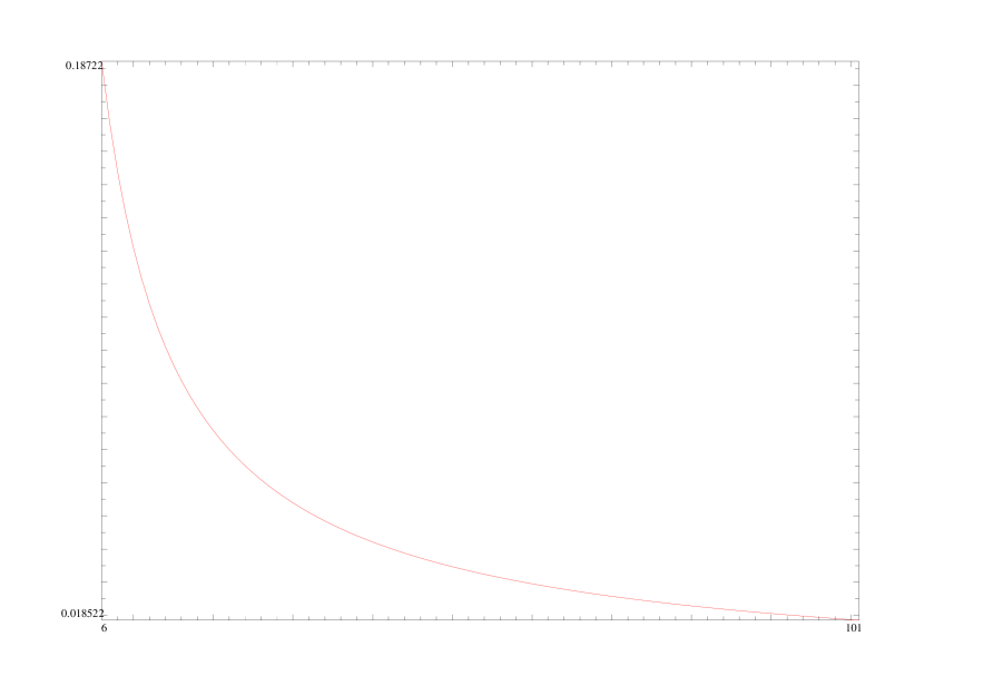
Figure 2: Plot of $a(u)-b(u)=(\log(\rho(u))-\log(\int_{u}^{\infty}\rho(x){\rm d}x))/u$ for $u\in[6,101]$.

Taking a logarithm, we define $b(u)=\log(e^{\gamma}-I(u))/u+\log(u)$, with $0>a(u)>b(u)$ for $u\geq 6$ and $b(100)\approx\log(1.5438\times 10^{-30})/100\approx-0.68643$. Fig. 2 gives a plot of $a(u)-b(u)$ for $u\in[6,101]$.

4.2 Oscillations of the Mertens discrepancy

Following Furry, we study the Mertens discrepancy $\Delta(u)=(u+1)e^{-\gamma}-\sigma(u)$. Lindemann remarked that the primes make $\Delta(1)=2e^{-\gamma}-1\approx 0.12292$ positive. Furry showed that rough semiprimes make $\Delta(2)=3e^{-\gamma}-1-\log(2)\approx-8.7687\times 10^{-3}$ negative. His polylogarithm $P_{2}(3)=\log(2)\log(\frac{3}{2})-\frac{1}{2}{\rm Li}_{2}(\frac{1}{4})$, at weight 2 for rough numbers with 3 prime divisors, gives the small positive value

$$\Delta(3)=4e^{-\gamma}-1-\log(3)-P_{2}(3)\approx 4.9686\times 10^{-6}.$$ (43)

Let $u_{n}$ be the $n$-th solution to $\Delta(u)=0$ with $u>1$. Then $u_{1}\approx 1.4833$ solves $(u+1)e^{-\gamma}=1+\log(u)$ and $u_{2}\approx 2.2270$ solves $(u+1)e^{-\gamma}=1+\log(u)+P_{2}(u)$, with a dilogarithm in (7), The next three zeros occur at $u_{3}\approx 3.0017$, $u_{4}\approx 3.7858$ and $u_{5}\approx 4.5665$. Their locations can be found at high precision using Theorems 4 and 5. Thereafter we use Algorithm 2, which gives 250 good digits, for $u_{6}\approx 5.3507$ up to $u_{25}\approx 20.776$, in about a minute. The extrema are easy to locate, since $u\Delta^{\prime}(u)=\Delta(u-1)$ for $u>1$. The minimum value of $\Delta(u)$ is $\Delta(e^{\gamma})=e^{-\gamma}-\gamma=-0.015756$. Thereafter, diminishing local extrema occur at $u=u_{n}+1$.

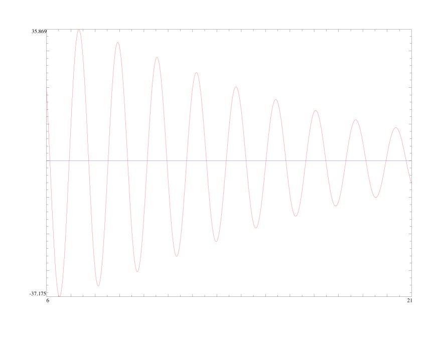
Figure 3: Oscillations of $\Delta(u)/\rho(u+3)$ for $u\in[6,21]$.

The oscillations of $\Delta(u)$ are damped super-exponentially, with $|\Delta(u)|<u^{-u}$ for $u\geq 1$. In Fig. 3 we have divided $\Delta(u)$ by $\rho(u+3)$, to moderate the damping.

4.3 Filtration by weight

$u\,\backslash k$	0	1	2	3	4	5	6	7	8	9
2	591	409
3	445	489	66
4	356	494	145	5
5	297	478	203	22	0
6	254	456	243	44	2	0
7	223	433	271	67	6	0	0
8	198	412	291	88	11	1	0	0
9	178	391	304	107	18	1	0	0	0
10	162	373	313	125	25	3	0	0	0	0
20	85	254	315	218	95	27	5	1	0	0
30	57	195	287	246	139	55	16	4	1	0
40	43	160	261	253	166	79	28	8	2	0
50	35	137	239	253	183	97	40	13	3	1
60	29	120	221	249	194	112	50	18	5	1
70	25	107	206	245	202	124	59	23	7	2
80	22	96	193	239	207	134	68	28	9	3
90	20	88	182	234	210	142	76	33	12	4
100	18	81	173	228	212	149	82	37	14	4

Table 1: Rounded contributions to $\sigma(u)$ of $P_{k}(u)$ in parts per thousand.

Following de Bruijn’s astute work [15, 16, 17], written almost a decade after the Lindemann–Furry letters [38, 52], subsequent authors [24, 35, 36, 55, 58] have studied the behaviour of $\rho(u)$ and $\sigma(u)$, with the latter perhaps disguised by de Bruijn’s definition [15] of $\omega(u)=\sigma^{\prime}(u)=\sigma(u-1)/u$, for $u>1$. We recover information that may have been overlooked: the filtration by weight begun by Furry.

The filtration $\sigma(u)=\sum_{u>k\geq 0}P_{k}(u)$ appeals to us, as physicists, because $P_{k}(u)$ is commendably concrete. It estimates the density, relative to the primes, of large rough numbers of size $N$ that are products of $k+1$ primes, the smallest of which satisfies $p^{u+1}>N$. Table 1 rounds $10^{3}P_{k}(u)/\sigma(u)$, showing the contribution by weight, in parts per thousand, for some integer values of $u\in[2,100]$. It is notable that the modal weight is less than 4 for $u\leq 100$. Table 2 indicates how the mean and standard deviation of the distribution by weight change with $u$.

$u$	10	20	30	40	50	60	70	80	90	100
mean	1.4867	2.0916	2.4660	2.7378	2.9513	3.1272	3.2767	3.4068	3.5218	3.6250
s.d.	1.0039	1.2399	1.3724	1.4630	1.5313	1.5857	1.6308	1.6692	1.7025	1.7320

Table 2: Approximate means and standard deviations of weight distributions.

In the tails of the distributions by weight, we encounter $P_{k}(k+y)$ with $y=O(1)$. Such terms are tiny for large $k$ and small $y$, being suppressed by the square of a factorial, with $(k!)^{2}P_{k}(k+y)=y^{k}(1+O(y))$ and $P_{k}(k+1)<1/(k!)^{2}$ for all $k>0$. At $u=101$, the small Mertens discrepancy $|\Delta(101)|\approx 1.2931\times 10^{-244}$ is much larger than its weight 100 contribution, namely $P_{100}(101)\approx 4.3068\times 10^{-317}$. The last 4 terms in the sum over weights give a contribution $\sum_{k=1}^{4}P_{101-k}(101)\approx 6.0106\times 10^{-248}$ that is significantly smaller than $|\Delta(101)|$.

4.4 Inclusion of weights up to 200

$u\,\backslash k$	0	1	2	3	4	5	6	7	8	9	10	11
110	16	75	164	223	213	155	89	41	16	5	2	0
120	15	70	157	218	214	159	94	46	18	6	2	0
130	14	66	150	213	214	164	99	49	21	7	2	1
140	13	62	144	208	214	167	104	53	23	8	3	1
150	12	59	138	204	213	170	108	57	25	9	3	1
160	11	56	133	200	213	173	112	60	27	10	3	1
170	10	53	129	196	212	175	116	63	29	11	4	1
180	10	51	125	192	211	177	119	66	31	12	4	1
190	9	49	121	188	210	179	122	69	33	13	5	1
200	9	47	117	185	209	181	125	72	35	14	5	2

Table 3: Further contributions to $\sigma(u)$ of $P_{k}(u)$ in parts per thousand.

$u$	110	120	130	140	150	160	170	180	190	200
mean	3.7185	3.8040	3.8828	3.9558	4.0239	4.0876	4.1475	4.2040	4.2575	4.3083
s.d.	1.7582	1.7820	1.8036	1.8235	1.8418	1.8588	1.8746	1.8895	1.9034	1.9166

Table 4: Further means and standard deviations of weight distributions.

Tables 3 and 4 extend Tables 1 and 2 to $u=200$. At $u=201$ the weight 200 Furry probability $P_{200}(201)\approx 5.9733\times 10^{-751}$ makes a very small contribution to

$$\rho(201)=\sum_{k=0}^{200}(-1)^{k}P_{k}(201) \approx 6.7083\times 10^{-534}$$ (44)

$$e^{\gamma}-\sum_{n=1}^{201}n\sum_{k=0}^{n-1}(-1)^{k}P_{k}(n) \approx 9.1972\times 10^{-535}$$ (45)

$$202\,e^{-\gamma}-\sum_{k=0}^{200}P_{k}(201) \approx 7.7106\times 10^{-552}$$ (46)

for each of which we have obtained more than 400 significant figures.

5 Statistics of factorization

Here we study ranges of reasonably large integers, $n\in[N_{1},N_{2}]$, and count primes, semiprimes and, crucially, integers with precisely three (not necessarily distinct) prime factors, which for convenience we call triprimes, as suggested by John Conway (1937–2020). We choose ranges that are relatively narrow, with $N_{2}\gg(N_{2}-N_{1})\gg 1$.

Counting primes is easier than counting semiprimes or triprimes. Consider the modest case with $N_{2}=10^{24}$ and $N_{2}-N_{1}=552750053$, which contains $c_{0}=10^{7}$ primes, the smallest of which is $N_{1}$. One expects about $(N_{2}-N_{1})/\log(N_{2})\approx 10002346$ primes from the prime number theorem. To count the primes, we first remove all integers with a prime divisor $p<N_{2}^{1/4}=10^{6}$. This is easily done, by crossing out arithmetic progressions in a bitmap. There remain 22463197 rough integers. This accords fairly well with a Mertens estimate $4e^{-\gamma}c_{0}\approx 22458379$.

There are $c_{1}+c_{2}=12463197$ composite integers that get through the sieve. These comprise $c_{1}$ semiprimes, $n=p_{0}p_{1}$, with $10^{6}<p_{0}\leq p_{1}<10^{18}$, and $c_{2}$ triprimes, $n=p_{0}p_{1}p_{2}$, with $10^{6}<p_{0}\leq p_{1}\leq p_{2}<10^{12}$. Prime hunters discard these composite numbers, using a probable-primality test, such as ispseudoprime in Pari/GP, or an equivalent in dedicated software, such as OpenPFGW [64]. Any number that fails such a test is certainly composite [28]. Often no attempt is made to count semiprimes, or triprimes. In this modest range, it is not hard to do so. There are $c_{0}=10^{7}$ primes, $c_{1}=10992988$ semiprimes and $c_{2}=1470209$ triprimes.

Furry’s letter to Nature [38] tells us to expect that $c_{1}/c_{0}\to\log(3)\approx 1.0986$ and that $c_{2}/c_{0}\to P_{2}(3)=\log(2)\log(\frac{3}{2})-\frac{1}{2}{\rm Li}_{2}(\frac{1}{4})\approx 0.14722$, asymptotically, provided that we make very large counts, $c_{k}$. Allowing for variations of order $\sqrt{c_{k}}$, with limited statistics, Furry’s asymptotic predictions, based on continuous analysis, compare quite well with our modest data for numbers of size merely $10^{24}$, in a range with merely $10^{7}$ primes.

We repeated this process in a case with $N_{2}=10^{36}$, where distinguishing a rough semiprime from a rough triprime requires considerably more work. Here we chose $N_{1}=N_{2}-82890279$, which gives $c_{0}=10^{6}$ primes, compared with an expectation of 999966, from the prime number theorem. Sieving out integers divisible by primes $p<N_{2}^{1/4}=10^{9}$, we were left with 2246578 rough numbers. Of these, $c_{1}=1099722$ are semiprimes and $c_{2}=146856$ are triprimes. Again, the agreement with Furry is acceptable, allowing for square-root uncertainties and sub-asymptotic effects.

6 Comments and conclusions

After formulating a now proven [71] conjecture (16) on Dickman polylogarithms and their asymptotic constants [14], one of us (DB) noted that Furry’s dilogarithm ${\rm Li}_{2}(\frac{1}{4})$ in (40) for the Mertens discrepancy [73] also appears at weight 2 in the Dickman problem. This led to historical research that appears, much condensed, in Section 3. The second author (SO) was led to Theorem 2 via the development of a path-integral approach to prime density. Our joint work synthesizes best practice in high-energy physics [72] with an efficient double-tail method [2, 3, 26] for multiple polylogarithms, for which we offer the following summary.

1. Theorems 1 and 2 solve the Dickman and Buchstab problems in parallel, with products of rapidly computable multiple polylogarithms (2) determining the Furry probabilities $P_{k}(u)$ of pure weight $k<u$ in the terminating series (6).

2. A one-off hour-long payment, for constants $P_{k}(n)$ with integers $k<n\in[1,101]$, is rewarded by fast computation of $P_{k}(u)$ for real $u>k$ in Algorithm 2, giving at least 100 significant figures for the Dickman and Buchstab functions with $u\in[1,101]$ and also their filtrations by weight.

3. For small $u-k$, Theorem 3 is efficient. For $k<5$, Theorems 4 and 5 are efficient. For $k<10$, one-dimensional quadrature based on Theorem 6 is efficient. For $k<u\in[10,201]$, the efficient $N$-step method of Algorithms 1 and 2 was used.

4. The asymptotic appearances of $e^{-\gamma}$ in the Buchstab problem and $e^{\gamma}$ in the Dickman problem provide strong tests of the accuracy and efficiency of the Akhilesh–Cohen algorithm in the procedure polylogmult of Pari/GP at weights up to 200 with 1000-digit working precision.

5. Tables 1 to 4 show distributions by weight, their means and standard deviations. Figures 1 to 3 show trends at large $u$ and oscillations about these.

6. Mindful that mathematics is a human activity, we have chronicled the roles of 6 interesting authors, of at least 4 nationalities, two of whom remain anonymous.

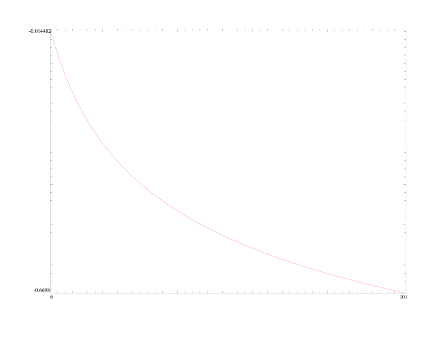
Figure 1: Plot of $a(u)=\log(\rho(u))/u+\log(u)<0$ for $u\in[6,101]$.

References

- [1] K. Acres and D. Broadhurst, Empirical determinations of Feynman integrals using integer relation algorithms, in Anti-Differentiation and the Calculation of Feynman Amplitudes, (ed. J. Blümlein and C. Scheider) pp 63–82, Springer, Cham, 2021. http://arxiv.org/abs/2103.06345
- [2] P. Akhilesh, Double tails of multiple zeta values, J. Number Theory 170 (2017), 228–249. http://arxiv.org/abs/2105.12156
- [3] P. Akhilesh, Multiple zeta values and multiple Apéry-like sums. http://arxiv.org/abs/1912.05204
- [4] E. Bach and R. Peralta, Asymptotic semismoothness probabilities, Math. Comp. 65 (1996), 1701–1715.
- [5] D. H. Bailey and D. J. Broadhurst, Parallel integer relation detection: techniques and applications, Math. Comp. 70 (2000), 1719–1736. http://arxiv.org/abs/math/9905048
- [6] R. Bellman and B. Kotkin, On the numerical solution of a differential-difference equation arising in analytic number theory, Math. Comp. 16 (1962), 473–475. http://www.jstor.org/stable/2003137
- [7] J. Blümlein, D. J. Broadhurst and J. A. M. Vermaseren, The multiple zeta value data mine, Comput. Phys. Commun. 181 (2010), 582–625. http://arxiv.org/abs/0907.2557
- [8] J. Blümlein and C. Schneider. Analytic computing methods for precision calculations in quantum field theory, Int. J. Mod. Phys. A33 (2018), 1830015. http://arxiv.org/abs/1809.02889
- [9] J. M. Borwein, D. M. Bradley and D. J. Broadhurst, Evaluation of -fold Euler/Zagier sums: a compendium of results for arbitrary , Elec. J. Combin. 4 (1997), R5. http://arxiv.org/abs/hep-th/9611004
- [10] J. M. Borwein, D. M. Bradley, D. J. Broadhurst and P. Lisonek, Combinatorial aspects of multiple zeta values, Elec. J. Combin. 5 (1998), R38. http://arxiv.org/abs/math/9812020
- [11] J. M. Borwein, D. M. Bradley, D. J. Broadhurst and P. Lisonek, Special values of multiple polylogarithms, Trans. Amer. Math. Soc. 353 (2001), 907–941. http://arxiv.org/abs/math/9910045
- [12] R. P. Brent, Factorization of the tenth Fermat number, Math. Comp. 68 (1999), 429–451.
- [13] L. J. F. Brimble and A. J. V. Gale, Editors of Nature, French Men of Science in Britain, Nature 146, No. 3690, 20 July 1940, 73. http://www.nature.com/articles/146073a0
- [14] D. Broadhurst, Dickman polylogarithms and their constants. http://arxiv.org/abs/1004.0519
- [15] N. G. de Bruijn, On the number of uncancelled elements in the sieve of Eratosthenes, Ned. Akad. Wetensch. Proc. A53 (1950), 803–812. http://dwc.knaw.nl/DL/publications/PU00018826.pdf
- [16] N. G. de Bruijn, On the number of positive integers and free of prime factors , Ned. Akad. Wetensch. Proc. A54 (1951), 50–60. http://pure.tue.nl/ws/portalfiles/portal/1793853/597499.pdf
- [17] N. G. de Bruijn, The asymptotic behaviour of a function occurring in the theory of primes, J. Indian Math. Soc. 15 (1951), 25–42. http://pure.tue.nl/ws/files/2416706/597496.pdf
- [18] V. Brun, Le crible d’Ératosthène et le théorème de Goldbach, Videnskapsselskapets Skrifter I, Mat.-naturv. Klasse 3 (1920), 1–36. http://archive.org/details/lecriblederatost00brun/
- [19] A. A. Buchstab, Asymptotische Abschätzung einer allgemeinen zahlentheoretischen Funktion, Mat. Sbornik 2 (1937), 1239–1246, in Russian. http://www.mathnet.ru/eng/sm5649
- [20] A. A. Buchstab, On an asymptotic estimate of the number of numbers of an arithmetic progression which are not divisible by relatively small prime numbers, Mat. Sbornik 28 (1951), 165–184, in Russian. http://www.mathnet.ru/eng/sm5598
- [21] A. A. Buchstab, list of publications in Russian at portal Math-Net.Ru. http://www.mathnet.ru/rus/person26559
- [22] J. Chamayou, A probabilistic approach to a differential-difference equation arising in analytic number theory, Math. Comp. 27 (1973), 197–203.
- [23] S. Charlton, H. Gangl, D. Radchenko and D. Rudenko, On the Goncharov depth conjecture and polylogarithms of depth two. http://arxiv.org/abs/2210.11938
- [24] A. Y. Cheer and D. A. Goldston, A differential delay equation arising from the sieve of Eratosthenes, Math. Comp. 55 (1990), 129–141.
- [25] S. D. Chowla and T. Vjayaraghvan, On the largest prime divisors of numbers, J. Indian Math. Soc. 11 (1947), 31–37.
- [26] H. Cohen, Computing multiple polylogarithms after Akhilesh, seminar at the Hausdorff Centre for Mathematics, Bonn, April 2018. http://www.youtube.com/watch?v=UGcswQ0AHkg
- [27] Coleshill Auxiliary Research Team, Origins of the SOE and Auxiliary Units. http://www.staybehinds.com/origins-of-soe-and-auxiliary-units
- [28] R. Crandall and C. Pomerance, Prime Numbers: A Computational Perspective, Springer, Cham, 2005.
- [29] A. Dersy, M. D. Schwartz and X. Zhang, Simplifying polylogarithms with machine learning. http://arxiv.org/abs/2206.04115
- [30] K. Dickman, On the frequency of numbers containing prime factors of a certain relative magnitude, Arkiv Mat. Astron. Fys. 22 (1930), 1–14.
- [31] L. J. Dixon, O. Gurdogan, A J. McLeod and M. Wilhelm, Bootstrapping a stress-tensor form factor through eight loops. http://arxiv.org/abs/2204.11901
- [32] G. Farmelo, Churchill’s Bomb: A Hidden History of Britain’s First Nuclear Weapons Programme, Faber and Faber, UK, 2014.
- [33] Free French Scientist, Number of primes and probability considerations, Nature 148, No. 3762, 6 December 1941, 695. http://www.nature.com/nature/journal/v148/n3762/abs/148695a0.html
- [34] Free French Scientist, Obituary of Dr. F. Holweck, Nature 149, No. 3771, 7 February 1942, 695. http://www.nature.com/articles/149163b0
- [35] J. Friedlander, Integers free from large and small primes, Proc. London Math. Soc. 33 (1976), 565–576. http://doi.org/10.1112/plms/s3-33.3.565
- [36] J. Friedlander, A. Granville, A. Hildebrand and H. Maier, Oscillation theorems for primes in arithmetic progressions and for sifting functions, J. Amer. Math. Soc. 4 (1991), 25–86.
- [37] W. H. Furry, A symmetry theorem in the positron theory, Phys. Rev. 51 (1937), 125–129.
- [38] W. H. Furry, Number of primes and probability considerations, Nature 150, No. 3795, 25 July 1942, 120–121. http://www.nature.com/nature/journal/v150/n3795/abs/150120a0.html
- [39] A. B. Goncharov, Multiple polylogarithms, cyclotomy and modular complexes, Math. Res. Lett. 5 (1998). http://faculty.math.illinois.edu/K-theory/0297/arb98.pdf
- [40] R. Gregory, Science and World Order, Nature 148 (1941), 331; Conference on Science and World Order, Nature 148 (1941), 388–392. http://www.nature.com/articles/148388a0
- [41] J. Guéron, L’engagement dans la France Libre, Historical Archives of the European Union, JG.A-02. http://archives.eui.eu/en/fonds/154822?item=JG.A-02
- [42] J. B. S. Haldane, Number of primes and probability considerations, Nature 148, No. 3762, 6 December 1941, 694. http://www.nature.com/nature/journal/v148/n3762/abs/148694a0.html
- [43] G. H. Hardy and E. M. Wright, An Introduction to the Theory of Numbers, pp 21-22, Oxford University Press, UK, 5th edition, 1979.
- [44] A. Hildebrand, On the number of positive integers and free of prime factors , J. Number Theory 22 (1986), 289–307.
- [45] A. Hildebrand and G. Tenenbaum, Integers without large prime factors, Journal de théorie des nombres de Bordeaux 5 (1993), 411–484. http://www.numdam.org/item/JTNB_1993__5_2_411_0.pdf
- [46] Histoires de Français Libres ordinaires, Liste des Français Libres, ceux qui ont aidé le général de Gaulle de juin 1940 à août 1943. http://www.francaislibres.net/pages/page.php?id=1036
- [47] A. Hodges, Alan Turing: The Enigma, Burnett-Hutchinson, UK, 1983.
- [48] D. E. Knuth, The art of computer programming, Vol. 2, Semi-numerical algorithms, pp 382–384, Addison-Wesley, USA, 1998.
- [49] J. C. Lagarias, Euler’s constant: Euler’s work and modern developments, Bull. Amer. Math. Soc. 50 (2013), 527–628. http://arxiv.org/abs/1303.1856
- [50] L. Lewin, Polylogarithms and associated functions, North Holland, USA, 1981.
- [51] F. A. Lindemann, The unique factorization of a positive integer, Quarterly Journal of Mathematics 4 (1933), 319–320. http://doi.org/10.1093/qmath/os-4.1.319
- [52] F. A. Lindemann, Number of primes and probability considerations, Nature 148, No. 3754, 11 October 1941, 436. http://www.nature.com/nature/journal/v148/n3754/abs/148436a0.html
- [53] F. A. Lindemann, Number of primes and probability considerations, Nature 148, No. 3762, 6 December 1941, 695. http://www.nature.com/nature/journal/v148/n3762/abs/148695b0.html
- [54] F. A. Lindemann, Number of primes and probability considerations, Nature 150, No. 3795, 25 July 1942, 121. http://www.nature.com/nature/journal/v150/n3795/abs/150121a0.html
- [55] J. van de Lune and E. Wattel, On the numerical solution of a differential-difference equation arising in analytic number theory, Math. Comp. 23 (1969), 417–421.
- [56] R. S. Macrae, Winston Churchill’s Toyshop, Roundwood Press, UK, 1971.
- [57] L. Marks, Between Silk and Cyanide: A Codemaker’s War 1941–1945, Harper-Collins, UK, 1998.
- [58] G. Marsaglia, A. Zaman and J C. W. Marsaglia, Numerical solution of some classical differential-difference equations, Math. Comp. 53 (1989), 191–201.
- [59] F. Mertens, Ein Beitrag zur analytischen Zahlentheorie, J. reine angew. Math. 78 (1874), 46–62. http://eudml.org/doc/148244
- [60] S. Moch, P. Uwer and S. Weinzierl, Nested sums, expansion of transcendental functions and multi-scale multi-loop integrals, J. Math. Phys. 43 (2002), 3363–3386. http://arxiv.org/abs/hep-ph/0110083
- [61] P. Moree, Integers without large prime factors: from Ramanujan to de Bruijn. http://arxiv.org/abs/1212.1581
- [62] L. Naterop, A. Signer and Y. Ulrich, HandyG – rapid numerical evaluation of generalised polylogarithms in Fortran, Comput. Phys. Commun. 253 (2020), 107165. http://arxiv.org/abs/1909.01656
- [63] J. J. O’Connor and E. F. Robertson, Abraham Robinson, MacTutor History of Mathematics Archive, 2000. http://mathshistory.st-andrews.ac.uk/Biographies/Robinson/
- [64] OpenPFGW, pfgw.exe version 4.0.5.7, April 2023. http://sourceforge.net/projects/openpfgw/files/
- [65] PARI Group, Pari/GP version 2.15.3, March 2023. http://pari.math.u-bordeaux.fr/
- [66] A. R. Pears, Obituary of Edward Maitland Wright, Bull. London Math. Soc. 39 (2007), 857–865. http://doi.org/10.1112/blms/bdm067
- [67] N. W. Pirie, John Burdon Sanderson Haldane, Biographical Memoirs of Fellows of the Royal Society 12 (1966), 218–249. http://www.jstor.org/stable/769532
- [68] V. Ramaswami, On the number of positive integers less than and free of prime divisors greater than , Bull. Amer. Math. Soc. 55 (1949), 1122–1127.
- [69] E. Remiddi and J. A. M. Vermaseren, Harmonic polylogarithms, Int. J. Mod. Phys. A15 (2000), 725–754. http://arxiv.org/abs/hep-ph/9905237
- [70] J. Schwinger, Quantum electrodynamics III. The electromagnetic properties of the electron – radiative corrections to scattering, Phys. Rev. 76 (1949), 790–817.
- [71] K. Soundararajan, An asymptotic expansion related to the Dickman function, Ramanujan J. 29 (2012), 25–30. http://arxiv.org/abs/1005.3494
- [72] J. Vollinga and S. Weinzierl, Numerical evaluation of multiple polylogarithms, Comput. Phys. Commun. 167 (2005), 177–194. http://arxiv.org/abs/hep-ph/0410259
- [73] S. Wagon, It’s only natural: the Mertens paradox, Math Horizons 13 (2005), 26–28. http://www.jstor.org/stable/25678567
- [74] E. M. Wright, Number theory and other reminiscences of Viscount Cherwell, Notes Rec. Roy. Soc. London 42 (1988), 197–204. http://rsnr.royalsocietypublishing.org/content/42/2/197
- [75] D. Zagier, Values of zeta functions and their applications, First European Congress of Mathematics, Vol. II, (Paris, 1992), Progr. Math. 120 (1994), 497–512. http://people.mpim-bonn.mpg.de/zagier/