A Wall-time Minimizing Parallelization Strategy for Approximate Bayesian Computation

Abstract

Approximate Bayesian Computation (ABC) is a widely applicable and popular approach to estimating unknown parameters of mechanistic models. As ABC analyses are computationally expensive, parallelization on high-performance infrastructure is often necessary. However, the existing parallelization strategies leave resources unused at times and thus do not optimally leverage them yet.

We present look-ahead scheduling, a wall-time minimizing parallelization strategy for ABC Sequential Monte Carlo algorithms, which utilizes all available resources at practically all times by proactive sampling for prospective tasks. Our strategy can be integrated in e.g. adaptive distance function and summary statistic selection schemes, which is essential in practice. Evaluation of the strategy on different problems and numbers of parallel cores reveals speed-ups of typically 10-20% and up to 50% compared to the best established approach. Thus, the proposed strategy allows to substantially improve the cost and run-time efficiency of ABC methods on high-performance infrastructure.

1 Introduction

The ultimate goal of systems biology is a holistic understanding of biological systems [1, 2]. Mechanistic models are important tools towards this aim, allowing to describe and understand underlying mechanisms [3]. Usually, such models have unknown parameters that need to be estimated by comparing model outputs to observed data [4]. For complex stochastic models, in particular multi-scale models used to describe the complex dynamics of multi-cellular systems, evaluating the likelihood of data given parameters however becomes quickly computationally infeasible [5, 6]. For this reason, simulation-based methods that circumvent likelihood evaluation have been developed, such as approximate Bayesian computation (ABC), popular for its simplicity and wide applicability [7, 8].

ABC generates samples from an approximation to the true Bayesian posterior distribution. While asymptotically exact, a known disadvantage of ABC is its reliance on repeated simulation, often hundred thousands to millions of times. Therefore, methods to efficiently explore the search space have been developed [9]. In particular, ABC is frequently combined with a Sequential Monte Carlo scheme (ABC-SMC), which over several generations successively refines the posterior approximation via importance sampling while maintaining high acceptance rates [10, 11]. Furthermore, in ABC-SMC the sampling for each generation can be parallelized, enabling the use of high-performance computing (HPC) infrastructure. This has in recent years enabled tackling increasingly complex problems via ABC [12, 13, 14, 15].

It would be desirable if available computational resources were perfectly exploited at all times, to minimize both the wall-time until results become available to the researcher, and the cost associated with allocated resources. However, the problem is that established parallelization strategies to distribute ABC-SMC work over a set of workers leave resources idle at times and thus fall short of this aim. The parallelization strategy used in most established HPC-ready ABC implementations is static scheduling (STAT), which defines exactly as many parallel tasks as accepted particles are required [16, 17]. While it minimizes the active compute time and consumed energy, typically a substantial amount of workers become idle towards the end of each generation. Dynamic scheduling (DYN) mitigates this problem and reduces the overall wall-time by continuing sampling on all workers until sufficiently many particles have been accepted [18]. It was shown to reduce the wall-time substantially. However, also in this strategy at the end of each generation workers become idle, waiting until all simulations have finished.

In this manuscript, we present a novel ABC-SMC parallelization strategy for multi-core and distributed systems, called look-ahead scheduling (LA). The strategy builds upon dynamic scheduling, but in addition, as workers get idle at the end of each generation, preemptively formulates tentative sampling tasks for the next generation. By this, it makes use of all available workers at almost all times. We show that by appropriate sample reweighting we obtain an unbiased Monte Carlo sample. We provide an HPC-ready implementation and test the method on various problems, demonstrating both efficiency and accuracy. Moreover, we show that the strategy can be integrated with adaptive algorithms for e.g. summary statistics, distance functions, or acceptance thresholds.

2 Methods

2.1 ABC

We consider a mechanistic model described via a generative process of simulating data $y\sim\pi(y|\theta)\in\mathbb{R}^{n_{y}}$ for parameters $\theta\in\mathbb{R}^{n_{\theta}}$. Given observed data $y_{\text{obs}}$, in Bayesian inference the likelihood $\pi(y_{\text{obs}}|\theta)$ is combined with prior information $\pi(\theta)$ to the posterior distribution $\pi(\theta|y_{\text{obs}})\propto\pi(y_{\text{obs}}|\theta)\cdot\pi(\theta).$ We assume that evaluating the likelihood is computationally infeasible, but that it is possible to simulate data $y\sim\pi(y|\theta)$ from the model. Then, classical ABC consists in the 3 steps of first sampling parameters $\theta\sim\pi(\theta)$, second simulating data $y\sim\pi(y|\theta)$, and third accepting $\theta$ if $d(y,y_{\text{obs}})\leq\varepsilon$, for a distance metric $d:\mathbb{R}^{n_{y}}\times\mathbb{R}^{n_{y}}\rightarrow\mathbb{R}_{\geq 0}$ and acceptance threshold $\varepsilon>0$. This is repeated until sufficiently many particles, say $N$, are accepted. The population of accepted particles constitutes a sample from an approximation of the posterior distribution,

$$\pi_{\mathrm{ABC},\varepsilon}(\theta|y_{\text{obs}})\propto\int I[d(y,y_{\text{obs}})\leq\varepsilon]\pi(y|\theta)\mathop{dy}\cdot\pi(\theta).$$ (1)

Under mild assumptions, $\pi_{\mathrm{ABC},\varepsilon}(\theta|y_{\text{obs}})$ converges to the actual posterior $\pi(\theta|y_{\text{obs}})$ as $\varepsilon\rightarrow 0$ [19, 20]. Commonly, ABC operates not directly on the measured data, but summary statistics thereof, capturing relevant information in a low-dimensional representation [21]. Here, for notational simplicity we assume that $y$ already incorporates summary statistics, if applicable.

2.2 ABC-SMC

The vanilla ABC formulation exhibits a trade-off between reducing the approximation error induced by $\varepsilon$, and high acceptance rates. Thus, ABC is frequently combined with a Sequential Monte Carlo scheme (ABC-SMC) [22, 23]. In ABC-SMC, a series of particle populations $P_{t}=\{(\theta_{t}^{i},w_{t}^{i})\}_{i\leq N}$ is generated, constituting samples of successively better approximations $\pi_{\mathrm{ABC},\varepsilon_{t}}(\theta|y_{\text{obs}})$ of the posterior, for generations $t=1,\ldots,n_{t}$, with acceptance thresholds $\varepsilon_{t}>\varepsilon_{t+1}$. In the first generation ($t=1$), particles are sampled directly from the prior, $g_{1}(\theta)=\pi(\theta)$. In later generations ($t>1$), particles are sampled from proposal distributions $g_{t}(\theta)\gg\pi(\theta)$ based on the last generation’s accepted weighted population $P_{t-1}$, e.g. via a kernel density estimate. The importance weights $w_{t}^{i}$ are the Radon-Nikodym derivatives $w_{t}(\theta)=\pi(\theta)/g_{t}(\theta)$. This is precisely such that the weighted parameters are samples from the distribution

$$\int w_{t}(\theta)I[d(y,y_{\text{obs}})\leq\varepsilon_{t}]\pi(y|\theta)\mathop{dy}\cdot g_{t}(\theta)=\int I[d(y,y_{\text{obs}})\leq\varepsilon_{t}]\pi(y|\theta)\mathop{dy}\cdot\pi(\theta),$$ (2)

i.e. the target distribution (1) for $\varepsilon=\varepsilon_{t}$.

Common proposal distributions first select an accepted parameter from the last generation and then perturb it, in which case $g_{t}$ takes the form $g_{t}(\theta)=\sum_{i=1}^{N}w_{t-1}^{i}K(\theta|\theta_{t-1}^{i})/\sum_{i=1}^{N}w_{t-1}^{i}$, with e.g. $K(\theta|\theta_{t-1}^{i})=\mathcal{N}(\theta|\theta_{t-1}^{i},\Sigma_{t-1})$ a normal distribution with mean $\theta^{i}_{t-1}$ and covariance matrix $\Sigma_{t-1}$. The performance of ABC-SMC algorithms relies heavily on the quality of the proposal distribution, on its ability to efficiently explore the parameter space. Methods that adapt to the problem structure, e.g. basing $\Sigma_{t-1}$ on the previous generation’s weighted sample covariance matrix and potentially localizing around $\theta_{i}$, have shown superior [24, 25, 26]. The steps of ABC-SMC are summarized in Algorithm 1.

for $t=1,\ldots,n_{t}$ do

       set $g_{t}$ and $\varepsilon_{t}$

       while less than $N$ acceptances do

             sample parameter $\theta\sim g_{t}(\theta)$

             simulate data $y\sim p(y|\theta)$

             accept $\theta$ if $d(y,y_{\text{obs}})\leq\varepsilon_{t}$

            

      compute weights $w_{t}^{i}=\frac{\pi(\theta_{t}^{i})}{g_{t}(\theta_{t}^{i})}$, for accepted parameters $\{\theta_{t}^{i}\}_{i\leq N}$

Algorithm 1 ABC-SMC algorithm.

The output of ABC-SMC is a population of weighted parameters

$$P_{n_{t}}=\{(\theta_{n_{t}}^{i},w_{n_{t}}^{i})\}_{i\leq N}\sim\pi_{\mathrm{ABC},\varepsilon_{n_{t}}}(\theta|y_{\text{obs}}).$$

For a statistic $f:\mathbb{R}^{n_{\theta}}\rightarrow\mathbb{R}$, the expected value under the posterior is then approximated via the self-normalized importance estimator

$$\mathbb{E}_{\pi_{\mathrm{ABC},\varepsilon_{n_{t}}}(\theta|y_{\text{obs}})}[f]\approx\hat{f}=\sum_{i=1}^{N}W_{n_{t}}^{i}f(\theta_{n_{t}}^{i}),$$

which is asymptotically unbiased. Here, $W^{i}_{t}:=w^{i}_{t}/\sum_{j=1}^{N}w^{j}_{t}$ are self-normalized weights. This is necessary because the weights $w_{t}(\theta)=\pi(\theta)/g_{t}(\theta)$ are not normalized in the joint sample space $(\theta,y)$, therefore effectively another Monte Carlo estimator is employed for the normalization constant (for details see the Supplementary Information, Section 1.1).

In importance sampling, samples are assigned different weights, such that some impact estimates more than others. This can be quantified e.g. via the effective sample size (ESS) [27, 9]:

$$\operatorname{ESS}(\{w_{i}\}_{i\leq N})=\frac{(\sum_{i\leq N}w_{i})^{2}}{\sum_{i\leq N}w_{i}^{2}}$$ (3)

2.3 Established parallelization strategies

In ABC, often hundred thousands to millions of model simulations need to be performed, which is typically the computationally critical part. To speed up inference, parallelization strategies have been developed that exploit the independence of the $N$ particles constituting the $t$-th population. Suppose we have $W$ parallel workers, each worker being a computational processor unit e.g. in an HPC environment. There are two established techniques to parallelize execution over the workers:

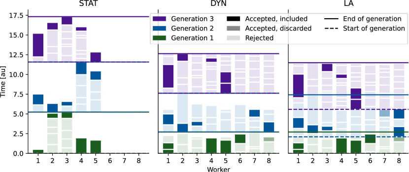
Figure 1: Illustration of core usage over run-time for static (STA), dynamic (DYN) and look-ahead (LA) scheduling for a population size $N=5$ on $W=8$ workers, over 3 generations (colors). The shading indicates whether a sample satisfies the acceptance criterion and is included in the final population (dark), satisfies the acceptance criterion but is discarded because enough earlier-started accepted samples exist (medium, for DYN+LA), or does not satisfy the acceptance criterion and is rejected (light). Solid lines indicate the end of a generation, dashed lines indicate the (preliminary) beginning of a generation (different from solid lines only for LA).

In static scheduling (STAT), given a population size $N$, $N$ tasks are defined and distributed over the workers. Each task consists in sampling until one particle gets accepted (Figure 1A). The tasks are queued if $N\geq W$. STAT minimizes the active computation time and number of simulations and is easy to implement, only requiring basic pooling routines available in most distributed computation frameworks. However, even for $W>N$ only $N$ workers are employed, although the number of required simulations is usually substantially larger than $N$. In addition, at the end of every generation the number of active workers decreases successively, most workers idly waiting for a few to finish their tasks. STAT is available in most established ABC-SMC implementations [17, 16].

In dynamic scheduling (DYN), sampling is performed continuously on all available workers until $N$ particles have been accepted (Figure 1B). However, simply taking those first $N$ particles as the final population would bias the population towards parameters with short-running simulations. Instead, in DYN all workers are waited for to finish, and out of the then $\tilde{N}\geq N$ accepted particles, only the $N$ that started earliest are considered accepted [18]. This ensures that acceptance probability of a particle is in accordance with the target distribution, independent of later events and thus its run-time.

2.4 Parallelization using look-ahead dynamic scheduling

DYN allows to exploit the available parallel infrastructure to a higher degree than STAT and therefore already substantially decreases the wall-time (by a factor of between 1.4 and 5.3 in test scenarios, see [18]). Nonetheless, some workers remain idle at the end of each generation while waiting for others to complete. This fraction increases as the number of workers increases relatively to the population size. Additionally, the idle time increases if simulation times are heterogeneous, which is often the case, e.g. with estimated reaction rates determining the number of simulated events (Supplementary Information, Section 3.6). In case of fast model simulations, also the time between generations, e.g. to post-process and store results, may be relatively long.

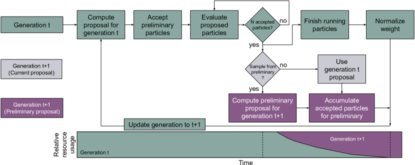
Figure 2: Concept visualization of look-ahead scheduling (LA). As soon as no more simulations are required for generation $t$ (green), a preliminary simulation task for generation $t+1$ is formulated either based on generation $t$ (dark purple) or $t+1$ (light purple). Resulting simulations are considered when evaluating the next generation ($t=t+1$), and suitable weight normalization is applied to all samples (top right). Over time, the number of workers dedicated to generation $t$ decreases, while that for generation $t+1$ increases (bottom).

2.4.1 Proposed algorithm

We propose to extend dynamic scheduling by using the free workers at the end of each generation to proactively sample for the next generation (Figure 2): As soon as $N$ acceptances have been reached in generation $t-1$ and workers thus start to get idle, we construct a preliminary proposal $\tilde{g}_{t}$, based on which particles for generation $t$ are generated and simulations performed on the free workers. $\tilde{g}_{t}$ can be based on a preliminary population of accepted particles $\hat{P}_{t-1}=\{(\hat{\theta}_{t-1}^{i},\hat{w}_{t-1}^{i})\}_{i\leq N}$ based on these first $N$ acceptances. However, $\hat{P}_{t-1}$ may introduce a practical bias (in a finite sample sense) towards particles with faster simulations times. This can in particular occur when computation time is highly parameter-dependent. To address this issue, the preliminary proposal can alternatively be based on $P_{t-2}$ (such that $\tilde{g}_{t}=g_{t-1}$), giving inductively practically unbiased proposals. If a particle $\tilde{\theta}_{t}\sim\tilde{g}_{t}$ gets accepted according to the acceptance criteria of generation $t$, its non-normalized weight is calculated as $\tilde{w}_{t}(\tilde{\theta}_{t})=\frac{\pi(\tilde{\theta}_{t})}{\tilde{g}_{t}(\tilde{\theta}_{t})}$. As soon as all simulations for generation $t-1$ have finished and thus the actual $P_{t-1}$ is available, all workers are updated to continue working with the actual sampling task based on proposal $g_{t}$. As the time-critical part of typical ABC applications is the model simulation, the cost of generating the preliminary sampling task is usually negligible.

The assessment of acceptance of preliminary samples depends on whether everything is pre-defined: If the acceptance components, including distance function $d$ and acceptance threshold $\varepsilon_{t}$ for generation $t$ are defined a-priori, then acceptance can be checked directly on the workers without knowledge of the complete previous population $P_{t-1}$. If however any component of the algorithm is adaptive and hence based on $P_{t-1}$ (e.g. the acceptance threshold is commonly chosen as a quantile of $\{d(y_{t-1}^{i},y_{\text{obs}})\}_{i\leq N}$), the acceptance check must be delayed until the actual $P_{t-1}$ is available. This serves to use one common acceptance criterion across all particles within a generation, so that all particles target the same distribution.

The population of generation $t$ is then, corrected for run-time bias as in DYN by only considering the $N$ accepted particles that were started first, given as

$$P_{t}=\{\{(\tilde{\theta}_{t}^{i},\tilde{w}_{t}^{i})\}_{i\leq\tilde{N}},\{(\theta_{t}^{i},w_{t}^{i})\}_{\tilde{N}<i\leq N}\},$$ (4)

with $0\leq\tilde{N}\leq N$ particles based on the preliminary proposal $\tilde{g}_{t}$, and $N-\tilde{N}$ on the final $g_{t}$. The weights need to be normalized appropriately, as explained in the following section. We call this parallelization strategy, which during generation $t-1$ already looks ahead to generation $t$, Look-ahead (dynamic) scheduling (LA).

2.4.2 Weights and unbiasedness

A key property of ABC methods is that they provide an asymptotically unbiased Monte Carlo sample from $\pi_{\mathrm{ABC},\varepsilon_{n_{t}}}(\theta|y_{\text{obs}})$, with $\pi_{\mathrm{ABC},\varepsilon_{n_{t}}}(\theta|y_{\text{obs}})\rightarrow\pi(\theta|y_{\text{obs}})$ for $\varepsilon\rightarrow 0$. The sample (4) obtained via LA conserves this property: The point is that each subpopulation on its own gives an asymptotically unbiased estimator, since the weights $\tilde{w}_{t}(\tilde{\theta})=\pi(\tilde{\theta})/\tilde{g}_{t}(\tilde{\theta})$, $w_{t}(\theta)=\pi(\theta)/g_{t}(\theta)$ are exactly the Radon-Nikodym derivatives w.r.t. the respective proposal distributions. These estimates are then combined, which decreases the Monte Carlo error due to the larger sample size. Instead of simply tossing all samples together, it is preferable to first normalize the weights relative to their subpopulation, $\tilde{W}^{i}_{t}:=\tilde{w}^{i}_{t}/\sum_{i=1}^{\tilde{N}}\tilde{w}^{j}_{t}$, $W^{i}_{t}:=w^{i}_{t}/\sum_{i=\tilde{N}+1}^{N}w^{i}_{t}$ (Supplementary Information, Section 1.3). This is because both weight functions are non-normalized, with generally different normalization constants, which renders them not directly comparable. A joint estimate based on the full population can then be given as

$$\mathbb{E}_{\pi_{\mathrm{ABC},\varepsilon_{t}}(\theta|y_{\text{obs}})}[f]\approx\beta\sum_{i=1}^{\tilde{N}}\tilde{W}^{i}_{t}f(\tilde{\theta}^{i}_{t})+(1-\beta)\sum_{i=\tilde{N}+1}^{N}W^{i}_{t}f(\theta^{i}_{t})$$ (5)

with $\beta\in[0,1]$ a free parameter. A straightforward choice is $\beta=\tilde{N}/N$, rendering the contribution of each subpopulation proportional to the respective number of samples. Instead, we propose to choose it to maximize the overall effective sample size (3), rendering the Monte Carlo estimate more robust. This is a simple constrained optimization problem with solution

$$\beta=\frac{\operatorname{ESS}(\{\tilde{W}^{i}_{t}\}_{i\leq\tilde{N}})}{\operatorname{ESS}(\{\tilde{W}^{i}_{t}\}_{i\leq\tilde{N}})+\operatorname{ESS}(\{W^{i}_{t}\}_{\tilde{N}<i\leq N})}$$

i.e. the contribution of each subpopulation is proportional to its effective sample size (Supplementary Information, Section 1.4). Supposing that for $N\rightarrow\infty$, $\tilde{N}/N\rightarrow\alpha\in[0,1]$, (5) converges to the left-hand side, as required. A more detailed derivation and extension to more than two proposal distributions is given in the Supplementary Information, Section 1.

2.5 Implementation and availability

We implemented LA in the open-source Python tool pyABC [28], which already provided STAT and DYN. We employ a Redis low-latency server to handle the task distribution. If all components are pre-defined, we perform evaluation of the “look-ahead” samples $(\tilde{\theta},\tilde{y})$ directly on the workers. If there are adaptive components, the delayed evaluation is performed on the main process. To avoid generating unnecessarily many preliminary samples in the presence of some very long-running simulations, we limited the number of preliminary samples to a default value of 10 times the number of samples in the current iteration. To not start preliminary sampling unnecessarily, we employed schemes predicting whether any termination criterion will be hit after the current generation. The code underlying this study can be found at https://github.com/EmadAlamoudi/Lookahead_study. A snapshot of code and data can be found at https://doi.org/10.5281/zenodo.7875905.

3 Results

Wall-time superiority of DYN over STAT has already been established in prior work [18]. To study the performance of LA and compare it to DYN, we applied both to several parameter estimation problems and in various scenarios of population size $N$ and workers $W$. We distinguish between “LA Pre” using the preliminary $\hat{P}_{t-1}$ to generate $\tilde{g}_{t}$, and “LA Cur” using $P_{t-2}$ instead.

3.1 Test problems

Table 1: Overview of application examples

ID	Description	Implementation	$n_{\theta}$
T1	Bimodal run-time-skewed model	Python	1
T2	Conversion reaction ODE model	Python	2
M1	Tumor spheroid growth [12]	C++	7
M2	Liver tissue regeneration [29]	Morpheus	14

We considered four problems (Table 1): Problems T1-T2 are simple test problems, while M1-M2 are realistic application examples.

Problem T1 is a bimodal model $y\approx\theta^{2}$, in which simulations from one mode have an artificially longer run-time, reflecting parameter dependence of run-times. Problem T2 is an ordinary differential equation (ODE) model with 2 parameters describing a conversion reaction $x_{1}\leftrightarrow x_{2}$, with observables obscured by random multiplicative noise. To analyze sampler behavior under simulation run-time heterogeneity, we added random log-normally distributed delay times $t_{\text{sleep}}$ of various variances atop the ODE simulations. For this model, run-times are fast, permitting repeated analysis to check correctness of the method, quantify stochastic effects and assess average behavior. Problem M1 describes the growth of a tumor spheroid using a hybrid discrete-continuous approach, modeling single cells as stochastically interacting agents and extracellular substances via PDEs [12]. Problem M2 describes the metabolic status of mechano-sensing during liver generation, describing the reaction network dynamics by a set of ODEs [29].

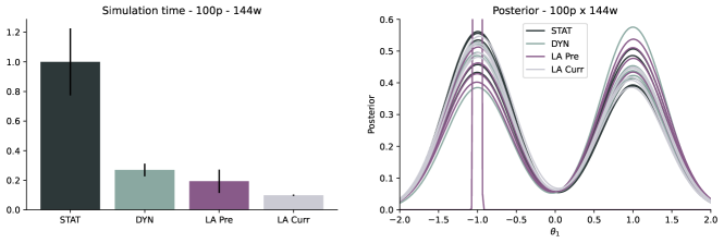
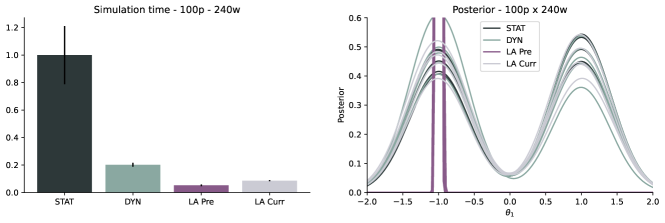
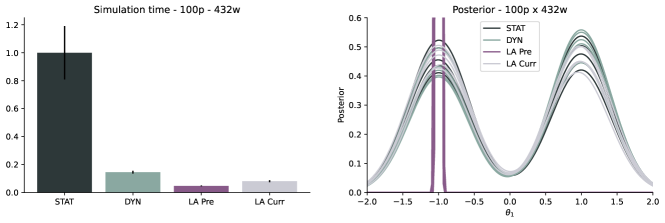
Figure 3: Run-time and posterior approximation for 5 different runs of model T1 with STAT, DYN, LA Pre and LA Cur, with population size $N=100$ on $W=144,240,432$ workers.

3.2 Biased proposal can induce practical bias in accepted population

The analysis of test model T1 revealed that for small population sizes $N$ relative to the number of workers $W$, together with high acceptance rates, LA Pre can indeed lead to a bias towards short-running simulations (Figure 3 right). This can happen when $\hat{P}_{t-1}$ is only based on short-running simulations, and only proposes particles from that regime, enough of which are then accepted to form $P_{t}$. For $N\geq W$, this effect no longer arose, likely because given large population sizes and sampling from other modes with associated high importance weights eventually happened, and because low acceptance rates make it improbably that acceptances in $P_{t}$ only stem from $\hat{P}_{t-1}$.

3.3 Sampling from unbiased proposal solves bias

When replacing LA Pre by LA Cur, i.e. sampling from $P_{t-2}$ instead of $\hat{P}_{t-1}$, the bias no longer occurred (Figure 3 right). This is as expected, because $\tilde{g}_{t-2}$ is has no run-time bias. In practice, we did not encounter any such problems on the considered application examples, where results from DYN, LA Pre and LA Cur were highly consistent. Yet, LA Pre may fail in some situations, which also demonstrates that ABC-SMC algorithms are sensitive to potential bias in the proposal distribution. Thus, in the following, we focus on the stable LA Cur, showing pendants for LA Pre in the Supplementary Information.

3.4 Look-ahead sampling gives accurate results

We used problem T2 to analyze different scenarios, with population sizes $N$ from 20 to 1280, worker numbers $W$ from 32 to 256, and log-normally distributed simulation times of variances $\sigma^{2}$ from 1.0 to 4.0. We ran each scenario 13 times to obtain stable average statistics. We considered means and standard deviations as point and uncertainty measures.

Point estimates for DYN and LA converged to the same values across population sizes (Figure 4 A+B). The proportion of accepted LA samples in the final population originating from the preliminary distribution ranged from nearly 100% to 50% (LA Pre) and 20% (LA Cur), as expected decreasing for larger population sizes (Figure 4 E+F). The more pronounced decrease for LA Cur than LA Pre is reasonable because void of bias, $\hat{P}_{t-1}$ provides a better sampling distribution than $P_{t-2}$. Effective sample sizes were stable across DYN and LA (Figure 4 D). A higher run-time variance lead to an increase in accepted samples originating from the preliminary proposal distribution (Supplementary Information, Figure S1), which is expected, because greater heterogeneity in run-times raises the chance of encountering exceptionally long-running simulations, which DYN has to wait for, while LA proceeds already.

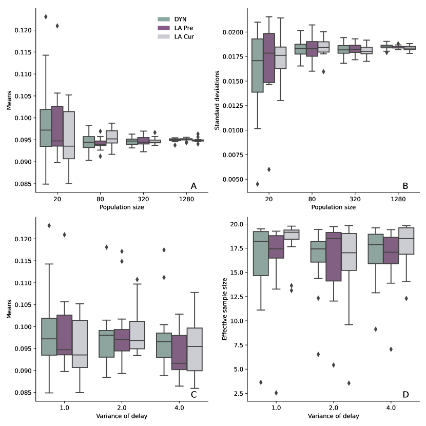
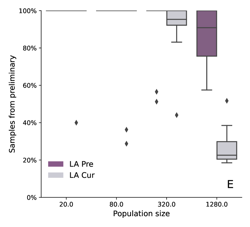
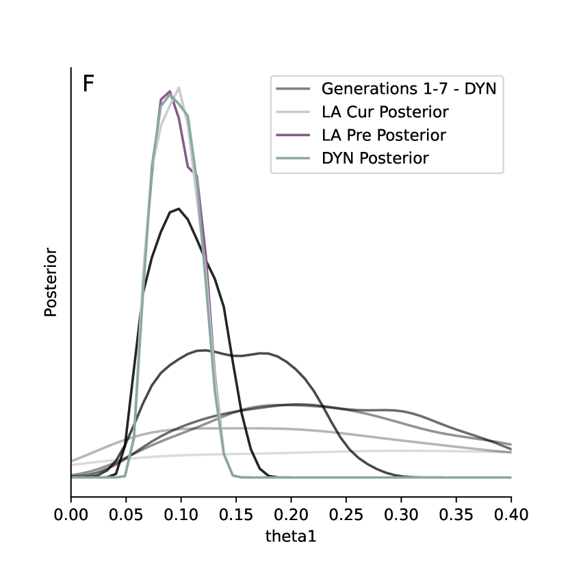
Figure 4: Results for problem T2 for different population sizes $N$, worker numbers $W$, and sleep time variances $\sigma^{2}$. Unless otherwise specified, we used $N=1280$, $W=256$, and a log-normally distributed sleep time $t_{\text{sleep}}$ of variance $\sigma^{2}=1$. To increase comparability, the $\varepsilon_{t}$ values over $n_{t}=8$ generations were pre-defined. (A) and (B): Mean and variance of the posterior approximation $\pi_{\mathrm{ABC},\varepsilon_{n_{t}}}(\theta|y_{\text{obs}})$. Box-plot over 13 repetitions. (C): Posterior mean for different sleep time variances, for $W=20$. (D): Effective sample size across different sleep time variances, for $N=256$ and $W=20$, in which case it is likely that several generations are sampled completely from the preliminary proposal. (E): Fraction $\tilde{N}/N$ of accepted samples in the final population $t=n_{t}$ that originate from the preliminary proposal $\tilde{g}_{n_{t}}(\theta)$ for LA Pre and LA Cur. (F): Exemplary visualization of 1d posterior approximation marginals for single runs.

3.5 Considerable speed-up towards high worker numbers

To analyze the effect of scheduling strategy on the overall wall-time, we ran model T2 systematically for different population sizes and numbers of workers . We considered population sizes $32\leq N\leq 1280$ and numbers of parallel workers $32\leq W\leq 256$, which covers typical ranges used in practice. Each scenario was repeated between $13$ times to assess average behavior, here we report mean values.

As a general tendency, the wall-time speed-up of LA over DYN became larger with increasing ratio of the number of workers by the population size. For a model sleep time variance of $\sigma^{2}=1$ (Figure 5), e.g. for $N=20$ and $W=256$, the average wall-time got reduced by a factor of almost 1.8. In most scenarios, a wall-time reduction by a factor of between $1.11$ and $1.8$ was observed. Only when the population size was large compared to the number of workers, was the speed-up comparably small.

For a sleep time variance of $\sigma^{2}=2$ (Supplementary Information, Figure S2), we observed similar behavior. There, the acceleration was generally more pronounced with up to a factor of roughly $1.9$ and many factors in the range $1.2$ to $1.9$. This indicates that indeed the advantage of LA over DYN is more pronounced in the presence of highly heterogeneous model simulation times.

Also on T1, the comparison of run-times (Figure 3 left) revealed a speed-up of LA over DYN. Further, we could confirm on both T1 and T2 (Figure 3 and Supplementary Information, Figure S3)the substantial speed-up DYN already provides over STAT, as reported in [18], on which we here improved further.

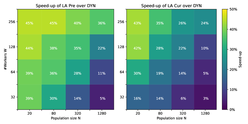
Figure 5: Speed-up ($1-\{\text{Wall-time LA}\}/\{\text{Wall-time DYN}\}$) of LA Pre (left) and LA Cur (right) over DYN for various population sizes and numbers of workers, for a model sleep time variance of $\sigma^{2}=1$.

3.6 Scales to realistic application problems

Given the high simulation cost of the application problems M1-2, we only performed selected analyses to compare LA and DYN. A reliable comparison of run-times in real-life application examples is challenging, because the total wall-time varies strongly due to stochastic effects, and computations are too expensive to perform inference many times.

For the two models, the parameter estimates obtained using LA (both LA Per and LA Cur) and DYN are consistent, up to expectable stochastic effects (Figures S4+5 and S9-11). Together with the previous analyses, this indicates that for practical applications, the multi-proposal approach of LA allows for stable and accurate inference, similar to the single proposal used by DYN. In early generations, a considerable part of the accepted particles was based on the preliminary proposal distribution (near 100%), which then decreased in later generations (Supplementary Information, Figures S6 and S12). This is consistent with the decrease in acceptance rate and thus the relative time during which the preliminary and not the final proposal distribution is used.

For the tumor model M1, we used an adaptive quantile-based epsilon threshold schedule [30], with DYN, LA Pre and LA Cur, population sizes $N\in\{250,500,1000\}$, and $W\in\{128,256\}$ workers. For each considered configuration we performed $2$ replicates (in total 8) to assess average behavior. Reported run-times are until a common final threshold was hit by all runs. The speed-up of LA over DYN varied depending on the ratio of population size and number of workers, similar to what we observed for T1+2. For high ratios, LA was consistently faster up to 35%. However, for low ratios, less improvement was observed. In some runs, LA was slightly slower than DYN (Figure 6). Over the 8 runs, we observed a mean speed-up of 21% (13%) and a median of 23% (16%) for LA Cur (LA Pre). This indicates expected speed-ups of 13-23%, however it should be remarked that large run-time differences and volatility could be traced back to single generations taking vast amounts of time (Supplementary Information, Figure S7). Those long generations occurred in all scheduling variants and exist most likely because the epsilon for that generation was chosen too optimistically, indicating a weakness of the used epsilon scheme, rather than the parallelization strategy.

For the liver regeneration model M2, we performed similar analyses, with adaptive quantile-based epsilon threshold schedules, population sizes $N\in\{250,500,1000\}$ and $W\in\{128,256\}$ workers, with 2 replicates per configuration. Similar to model M1, we observed a faster performance of up to 35%. However, with a smaller ratio between population size and the number of workers, a slightly lower performance improvement was achieved (Figure 7). Similarly to M1, the acceleration varied quite strongly. For LA Pre we observed a mean speed-up over all 8 runs of 36% (median 31%) over DYN. However, for LA Cur we observed contrarily a mean slow-down of 39% (median 43%) over DYN. It is not clear what caused this stark difference, which is again subject to high fluctuations. Further tests would be needed to assess the reasons for this specific model.

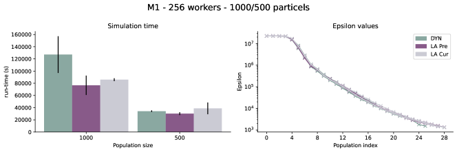
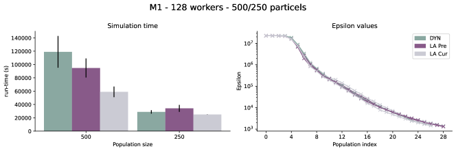
Figure 6: The run-time and posterior distributions for 2 different runs of the model (M1) with population size 1000, 500, 250 on 128 and 256 workers.

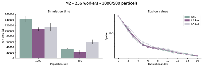
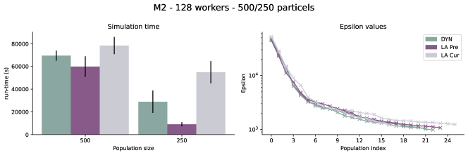
Figure 7: The run-time and posterior distribution of 2 different runs of the model (M2) with population size 1000, 500, 250 on 128 and 256 workers.

4 Discussion

Simulation-based ABC methods have made parameter inference increasingly accessible even for complex stochastic models, are however limited by computational costs. Here, we presented “look-ahead” sampling, a parallelization strategy to minimize wall-time by using all available high-performance computing resources at near-all times. On various test and application examples, we verified the accuracy and robustness of the novel approach in typical settings. Depending on model simulation run-time heterogeneity, and the relation of population size and the number of cores, we observed a speed-up of up to 45% compared to the previously most efficient strategy, dynamical scheduling. On typical application examples, we observed a speed-up of roughly 20-30%, however with some variability, assessing which would require further tests with considerable computational resources. We would also like to remark that ABC-SMC is sensitive to the choice of proposal distribution. Finite samples can induce a practical bias, as we observed here for parameter-dependent run-times of models – a problem that occurred in extreme cases but could only be solved by using look-ahead sampling with the previous, and not the preliminary, proposal distribution.

Conceptually and aside implementation details, the presented strategy provides the minimal wall-time among all parallelization strategies, as all cores are made use of at practically all times. We observed that look-ahead sampling using preliminary results (LA Pre) provided a performance speed-up over re-using the previous generation (LA Cur), however at the cost of practical bias. Were it possible to construct an unbiased proposal using those preliminary results, e.g. via reweighting or imbalance detection, we could thus increase the speed-up with robust performance. When using delayed evaluation, it would be possible to parallelize the evaluation as well, which we have not done here. If evaluation times are long relative to simulation times, e.g. if (adaptive) summary statistics involve complex operations, this would be beneficial. In order to reduce a potential bias in the preliminary proposal distribution towards fast-running simulations, it may be beneficial to update it as soon as more particles finish. This would imply the use of more than two importance distributions, the theory of which we have already provided in the Supplementary Information.

In conclusion, we showed how we can minimize wall-time and associated computing cost of ABC samplers with substantial performance gains over established methods. This concept is generally applicable for sequential importance sampling methods, thus we are certain that it will find widespread use.

Author contributions

JH and YS conceived the idea. YS, EA and FR developed and implemented the algorithms. EA and FR performed the case studies with assistance of NB and FG. EA, FG and LB developed the application problems. All authors discussed the results and jointly wrote and approved the manuscript.

References

- [1] H. Kitano. Systems biology: A brief overview. Science, 295(5560):1662–1664, 03 2002.
- [2] J. R. Karr, J. C. Sanghvi, D. N. Macklin, M. V. Gutschow, J. M. Jacobs, B. Bolival Jr, N. Assad-Garcia, J. I. Glass, and M. W. Covert. A whole-cell computational model predicts phenotype from genotype. Cell, 150(2):389–401, July 2012.
- [3] Neil A Gershenfeld and Neil Gershenfeld. The nature of mathematical modeling. Cambridge university press, 1999.
- [4] A. Tarantola. Inverse Problem Theory and Methods for Model Parameter Estimation. SIAM, 2005.
- [5] Simon Tavaré, David J Balding, Robert C Griffiths, and Peter Donnelly. Inferring coalescence times from DNA sequence data. Genetics, 145(2):505–518, 1997.
- [6] J. Hasenauer, N. Jagiella, S. Hross, and F. J. Theis. Data-driven modelling of biological multi-scale processes. J. Coupled Syst. Multiscale Dyn., 3(2):101–121, 9 2015.
- [7] Jonathan K Pritchard, Mark T Seielstad, Anna Perez-Lezaun, and Marcus W Feldman. Population growth of human y chromosomes: a study of y chromosome microsatellites. Mol. Biol. Evol., 16(12):1791–1798, 1999.
- [8] M. A. Beaumont, W. Zhang, and D. J. Balding. Approximate Bayesian Computation in Population Genetics. Genetics, 162(4):2025–2035, 12 2002.
- [9] Scott A Sisson, Yanan Fan, and Mark Beaumont. Handbook of approximate Bayesian computation. Chapman and Hall/CRC, 2018.
- [10] Pierre Del Moral, Arnaud Doucet, and Ajay Jasra. Sequential Monte Carlo samplers. J. R. Stat. Soc. B, 68(3):411–436, 2006.
- [11] S. A. Sisson, Y. Fan, and M. M. Tanaka. Sequential Monte Carlo without likelihoods. Proc. Natl. Acad. Sci., 104(6):1760–1765, Jan. 2007.
- [12] N. Jagiella, D. Rickert, F. J. Theis, and J. Hasenauer. Parallelization and high-performance computing enables automated statistical inference of multi-scale models. Cell Syst., 4(2):194–206, 02 2017.
- [13] Andrea Imle, Peter Kumberger, Nikolas D Schnellbächer, Jana Fehr, Paola Carrillo-Bustamante, Janez Ales, Philip Schmidt, Christian Ritter, William J Godinez, Barbara Müller, et al. Experimental and computational analyses reveal that environmental restrictions shape HIV-1 spread in 3D cultures. Nature Communications, 10(1):2144, 2019.
- [14] Karina Durso-Cain, Peter Kumberger, Yannik Schälte, Theresa Fink, Harel Dahari, Jan Hasenauer, Susan L. Uprichard, and Frederik Graw. HCV spread kinetics reveal varying contributions of transmission modes to infection dynamics. Viruses, 13(7), July 2021.
- [15] Emad Alamoudi, Yannik Schälte, Robert Müller, Jörn Starruß, Nils Bundgaard, Frederik Graw, Lutz Brusch, and Jan Hasenauer. Fitmulticell: Simulating and parameterizing computational models of multi-scale and multi-cellular processes. bioRxiv, 2023.
- [16] Ritabrata Dutta, Marcel Schoengens, Jukka-Pekka Onnela, and Antonietta Mira. Abcpy: A user-friendly, extensible, and parallel library for approximate Bayesian computation. In Proceedings of the Platform for Advanced Scientific Computing Conference, PASC ’17, pages 8:1–8:9, New York, NY, USA, 2017. ACM.
- [17] Antti Kangasrääsiö, Jarno Lintusaari, Kusti Skytén, Marko Järvenpää, Henri Vuollekoski, Michael Gutmann, Aki Vehtari, Jukka Corander, and Samuel Kaski. ELFI: Engine for Likelihood-Free Inference. In NIPS 2016 Workshop on Advances in Approximate Bayesian Inference, 2016.
- [18] Emmanuel Klinger, Dennis Rickert, and Jan Hasenauer. pyABC: distributed, likelihood-free inference. Bioinf., 34(20):3591–3593, 10 2018.
- [19] Richard David Wilkinson. Approximate Bayesian computation (ABC) gives exact results under the assumption of model error. Stat. Appl. Gen. Mol. Bio., 12(2):129–141, May 2013.
- [20] Yannik Schälte, Emad Alamoudi, and Jan Hasenauer. Robust adaptive distance functions for approximate Bayesian inference on outlier-corrupted data. bioRxiv, 2021.
- [21] Paul Fearnhead and Dennis Prangle. Constructing summary statistics for approximate Bayesian computation: semi-automatic approximate Bayesian computation. J. R. Stat. Soc. B, 74(3):419–474, 2012.
- [22] T. Toni, D. Welch, N. Strelkowa, A. Ipsen, and M. P. H. Stumpf. Approximate bayesian computation scheme for parameter inference and model selection in dynamical systems. J. R. Soc. Interface, 6:187–202, 7 2009.
- [23] Mark A Beaumont. Approximate bayesian computation in evolution and ecology. Annual review of ecology, evolution, and systematics, 41:379–406, 2010.
- [24] Mark A Beaumont, Jean-Marie Cornuet, Jean-Michel Marin, and Christian P Robert. Adaptive approximate bayesian computation. Biometrika, 96(4):983–990, 2009.
- [25] S. Filippi, C. P. Barnes, J. Cornebise, and M. P. Stumpf. On optimality of kernels for approximate Bayesian computation using sequential Monte Carlo. Stat. Appl. Genet. Mol., 12(1):87–107, 2013.
- [26] E. Klinger and J. Hasenauer. A scheme for adaptive selection of population sizes in Approximate Bayesian Computation - Sequential Monte Carlo. In J. Feret and H. Koeppl, editors, Computational Methods in Systems Biology. CMSB 2017, volume 10545 of Lecture Notes in Computer Science. Springer, Cham, 2017.
- [27] Jun S Liu, Rong Chen, and Wing Hung Wong. Rejection control and sequential importance sampling. J. Am. Stat. Assoc., 93(443):1022–1031, 1998.
- [28] Yannik Schälte, Emmanuel Klinger, Emad Alamoudi, and Jan Hasenauer. pyabc: Efficient and robust easy-to-use approximate bayesian computation. J. Open Source Softw., 7(74):4304, 2022.
- [29] Kirstin Meyer, Hernan Morales-Navarrete, Sarah Seifert, Michaela Wilsch-Braeuninger, Uta Dahmen, Elly M Tanaka, Lutz Brusch, Yannis Kalaidzidis, and Marino Zerial. Bile canaliculi remodeling activates yap via the actin cytoskeleton during liver regeneration. Mol. Syst. Biol., 16(2):e8985, 2020.
- [30] Christopher C Drovandi and Anthony N Pettitt. Estimation of parameters for macroparasite population evolution using approximate Bayesian computation. Biometrics, 67(1):225–233, 2011.