Speckle Interferometry with CMOS Detector

Abstract

In 2022 we carried out an upgrade of the speckle polarimeter (SPP)—the facility instrument of the 2.5-m telescope of the Caucasian Observatory of the SAI MSU. During the overhaul, CMOS Hamamatsu ORCA-Quest qCMOS C15550-20UP was installed as the main detector, some drawback of the previous version of the instrument were eliminated. In this paper, we present a description of the instrument, as well as study some features of the CMOS detector and ways to take them into account in speckle interferometric processing. Quantitative comparison of CMOS and EMCCD in the context of speckle interferometry is performed using numerical simulation of the detection process. Speckle interferometric observations of 25 young variable stars are given as an example of astronomical result. It was found that BM And is a binary system with a separation of 273 mas. The variability of the system is dominated by the brightness variations of the main component. A binary system was also found in NSV 16694 (TYC 120-876-1). The separation of this system is 202 mas.

1 INTRODUCTION

Passive methods for achieving diffraction limited angular resolution on ground-based telescopes, such as speckle interferometry, lucky imaging, differential speckle polarimetry, operate with a large number of short-exposure images of an object distorted by atmospheric turbulence (Labeyrie, 1970; Tokovinin, 1988). The need to ‘‘freeze’’ an image that changes with a characteristic time scale of $\tau_{0}$, called the atmospheric coherence time, determines the characteristic exposures that are applied: $(3$–$5)\tau_{0}=10$–$30$ ms.

In order to apply passive high angular resolution techniques to the observation of astronomical objects that typically have very low fluxes, it is critical to use detectors that have high quantum efficiency, high readout speed, and low readout noise. The last two qualities seem to be mutually exclusive, since faster output amplifier operation means higher readout noise, all other things being equal (Howell, 2000).

Various technologies have been used to overcome this contradiction, but a breakthrough was made with the invention in the late 1990s-early 2000s of the Electron Multiplying Charge–Coupled Device (EMCCD) (Basden & Haniff, 2004). EMCCDs differ from conventional CCD detectors by the presence of a special electron multiplication register between the horizontal register and the output amplifier. The electron multiplication register is a sequence of $N$ cells between which an increased potential is created. There is a probability $p_{\mathrm{EM}}\approx 10^{-3}$ that a photoelectron, passing between two successive cells of the electron multiplication register, will knock out one more electron. Passing through $N\approx 600$ cells of the electron multiplication register, the photoelectron turns into $G_{\mathrm{EM}}=(1+p_{\mathrm{EM}})^{N}$ electrons, on average, where $G_{\mathrm{EM}}$ is the so-called electron multiplication factor, which for commercially available EMCCDs can vary from 1 to 1000.

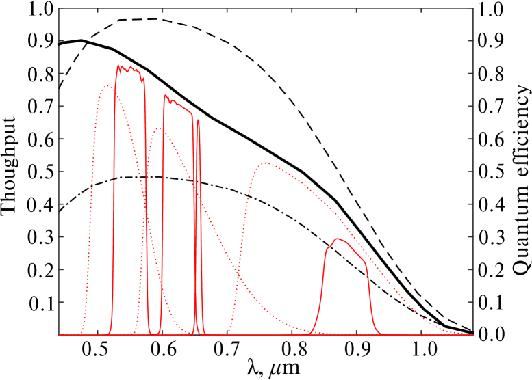
Figure 1: Quantum efficiency of detectors: EMCCD vs. CMOS, and transmission of filters. The dashed line is the quantum efficiency curve of the EMCCD Andor iXon 897 detector. The dash-dotted line is the same, but the quantum efficiencies are halved to account for amplification noise. The thick solid line is the quantum efficiency curve of the Hamamatsu ORCA-quest CMOS detector. The red lines are the transmission curves of the filters used in the speckle polarimeter multiplied by the Hamamatsu ORCA-quest quantum efficiency curve. The red dotted lines are broadband filters, from left to right: $V$, $R_{\mathrm{c}}$, $I_{\mathrm{c}}$. The red solid lines are midband filters: 550, 625, 656.3 (H_α), 880 nm.

Table 1: Parameters of detectors for speckle interferometry. The first column is EMCCD Andor iXon 897, a detector used in the speckle polarimeter from October 2015 to July 2022. The second and third columns are standard and ultra-quiet modes of the Hamamatsu ORCA-quest CMOS detector installed in the speckle polarimeter, starting from August 2022.

Parameter	Andor	Hamamatsu ORCA-quest
	iXon 897	standard	ultra-quiet
Technology	EMCCD	qCMOS
Dimensions, px	$512\times 512$	$4096\times 2304$
Pixel size, microns	16	4.6
RMSD of readout noise, $e^{-}$	48	0.43	0.27
Effective RMSD of readout noise, $e^{-}$	0.048	0.43	0.27
CIC, $e^{-}$/px	0.045	0
EM gain factor $G_{\mathrm{EM}}$	1–1000	1
Conversion factor, $e^{-}$/ADU	11.57	0.107
Register size, ADU	16 384	65 536
Potential well depth, $e^{-}$	180 000	7000
Frame rate (full frame), Hz	35	120	5
Frame rate (region $512\times 512$ px), Hz	35	532	22

Due to the fact that the signal is amplified before being digitized, the effective readout noise is reduced by a factor of $G_{\mathrm{EM}}$. In practice, the EMCCD readout noise is reduced to negligible values: $0.01$–$0.1e^{-}$. Strong suppression of readout noise makes it possible to use the output amplifier at frequencies that are orders of magnitude higher than the readout frequencies of classical CCDs: 10–30 MHz. The EMCCD is usually based on a back-illuminated chip and has a quantum efficiency of about 90% over a very wide wavelength range (see example in Fig. 1).

All of these properties have made EMCCD extremely popular for implementing speckle interferometry and similar methods (Law et al., 2006; Hormuth et al., 2008; Oscoz et al., 2008; Maksimov et al., 2009; Tokovinin et al., 2010; Scott et al., 2018). We also used the EMCCD Andor iXon 897 as the main detector of the speckle polarimeter, the facility instrument of the 2.5-m telescope of the Caucasian Observatory of the SAI MSU (Safonov et al., 2017), the detector parameters are given in Table 1.

EMCCDs have some known disadvantages. Firstly, this is the so-called amplification noise: the amplification process is stochastic in nature, and the actual electron multiplication factor for each particular photoelectron is a random variable. This is expressed as a twofold increase in the photon noise variance (Harpsøe et al., 2012). For conditions where photon noise is the dominant contributor to the total noise, this means that twice as many photons must be accumulated to achieve the same $S/N$ ratio.

Secondly, when the charge is clocked to the electron multiplication register, there is a non-zero probability that a spurious electron will appear (Clock-induced charge—CIC). This electron will be amplified and it will no longer be possible to distinguish it from the photoelectron knocked out by the source photon. For the iXon 897 detector used in the speckle polarimeter, the probability of registering a spurious electron is $0.045$/px.

Another significant disadvantage of EMCCDs is their low dynamic range. For example, when working with $G_{\mathrm{EM}}=500$, the maximum number of photons that can be registered by a given pixel before saturation is 350. The problem is aggravated by the fact that the use of a detector in conditions where at least one pixel is saturated leads to accelerated degradation of the electron multiplication register. Thus, the use of the standard CCD photometry strategy when bright stars are saturated, but this does not spoil the photometry of faint stars, turns out to be impossible for EMCCD.

Note that although in speckle interferometry we usually deal with one source per frame, the range of brightness in the speckle pattern is quite large. The value of the EM gain has to be chosen so that the brightest speckle is not saturated. If this gain turns out to be low, then for faint speckles, which are the majority, the detector operates with readout noise which is much larger than subelectron.

As an alternative to CCD detectors, CMOS detectors are used, which in recent years have been approaching, and in some cases even surpassing, CCDs in terms of performance. Technologically, CMOS, unlike CCD, reads each pixel individually. As a result, each specific ADC (Analog-to-Digital Converter) can operate relatively slowly, and, accordingly, have low readout noise.

Examples of the use of CMOS detectors in speckle interferometry can be found in Genet et al. (2016) and Wasson et al. (2017). However, the detectors used by the authors have a read noise of about $1{e}^{-}$ and are inferior to EMCCD.

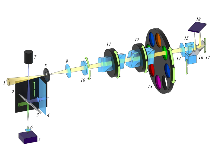
Figure 2: Instrument layout. 1—Beam from a telescope. The prefocal unit 2–8: the movable carriage 2, mirrors 3, one of the mirrors relays light from the telescope to the auxiliary camera (5–6), another mirror relays light from the calibration source (7) to the detector, 4—the linear polarizer, 8—the field aperture; the collimated beam unit 9–14: 9—the collimator, 10—the rotating half-wave plate, 11, 12—the prisms of the atmospheric dispersion compensator (the wedge angles are increased for clarity), 13—the filter wheel, 14—the lens; the camera unit 15–18: 15—the beam splitter, 16, 17—the relay mirrors, 18—the detector. The green arrows mark the motorized degrees of freedom.

In Table 1, we list the parameters of the Hamamatsu ORCA-Quest C15550-20UP CMOS detector (hereinafter simply Hamamatsu ORCA-Quest). It can be seen that the key characteristics important for speckle interferometry—read speed and readout noise—are comparable to EMCCD. Sub-electronic readout noise is achieved without amplification and therefore without the problems associated with it: amplification noise and low dynamic range.

In Fig. 1 we compare the quantum efficiency curves of Andor iXon 897 and Hamamatsu ORCA-Quest. It can be seen that the CMOS quantum efficiency curve is slightly lower than that of CCD, but this advantage disappears when the presence of amplification noise in the latter is taken into account.

The Hamamatsu ORCA-Quest detector was chosen by us as the main detector of the speckle polarimeter, which was installed instead of the EMCCD. The replacement of the detector required a significant overhaul of the instrument design. Taking advantage of this moment, we made several key changes along the way, which made it possible to increase the efficiency of speckle interferometric observations. Changes in instrument design are described in Section 2.

In Section 3, we describe some features of the application of CMOS in the context of speckle interferometry. We have performed a quantitative comparison of the efficiency of EMCCD and CMOS using our numerical measurement model (Section 4). Finally, in Section 5 we present some results of the study of the binarity of the UX Ori type stars, carried out both with EMCCD and CMOS. In particular, the binarity of BM And and NSV 16694 was discovered. In this article, we will not discuss the polarimetric mode of the instrument; this will be done in the future paper.

2 INSTRUMENT

The design of the speckle polarimeter was discussed in detail earlier in the article (Safonov et al., 2017). Here we will discuss, first of all, the changes that was applied in the context of the installation of Hamamatsu ORCA-quest as the main detector. The instrument consists of the following units: a prefocal unit, a collimated beam unit, a camera unit, a control electronics unit, a control computer (see Fig. 2 and Fig. 3).

Figure 3: General view of the instrument from the side of the main detector (render of CAD model). Direction to the telescope—to the right, flange to the telescope.

2.1 Prefocal unit

The prefocal unit (Fig. 4) performs a number of auxiliary functions. It contains an auxiliary CCD camera, onto which light from the telescope is relayed by introducing a diagonal mirror into the beam. The purpose of auxiliary camera is to center object when the telescope’s pointing error exceeds $15^{\prime\prime}$ and the object does not fit within the field of view of the main detector. Since 2022, we have been using an industrial black-and-white CCD detector Prosilica GC655 as an auxiliary camera, which made it possible to center objects up to $m_{V}=17^{\rm m}$. The camera has a field of view $70^{\prime\prime}$.

In addition, the prefocal unit includes a calibration source, which is represented by an array of holes with a diameter of 70 $\mu$m, with a step of 800 $\mu$m, illuminated by a white superbright LED through an additional diffuser. The image of the calibration source is relayed into the focal plane with $3.5\times$ demagnification through a two-lens achromat and a moving mirror (see Fig. 5a for an image example).

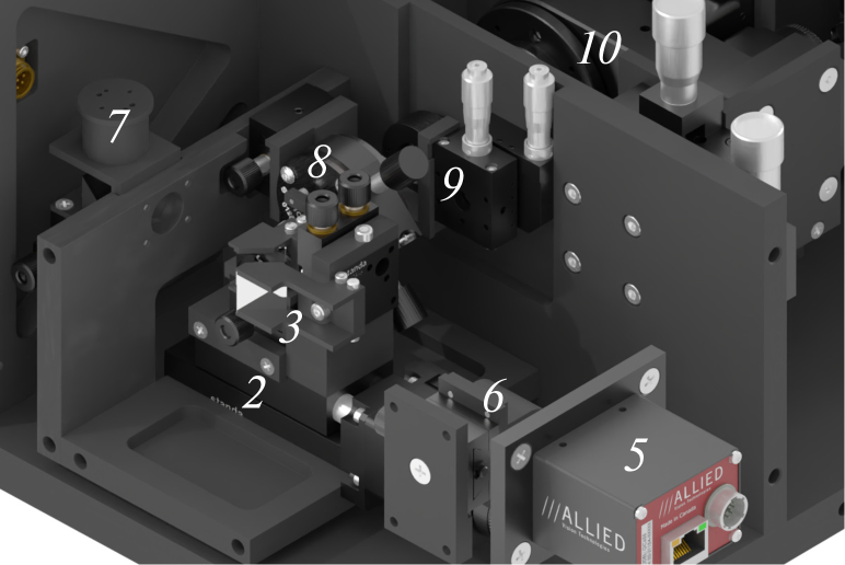
Figure 4: The prefocal unit (render of CAD model). The designations are the same as in Fig. 2.

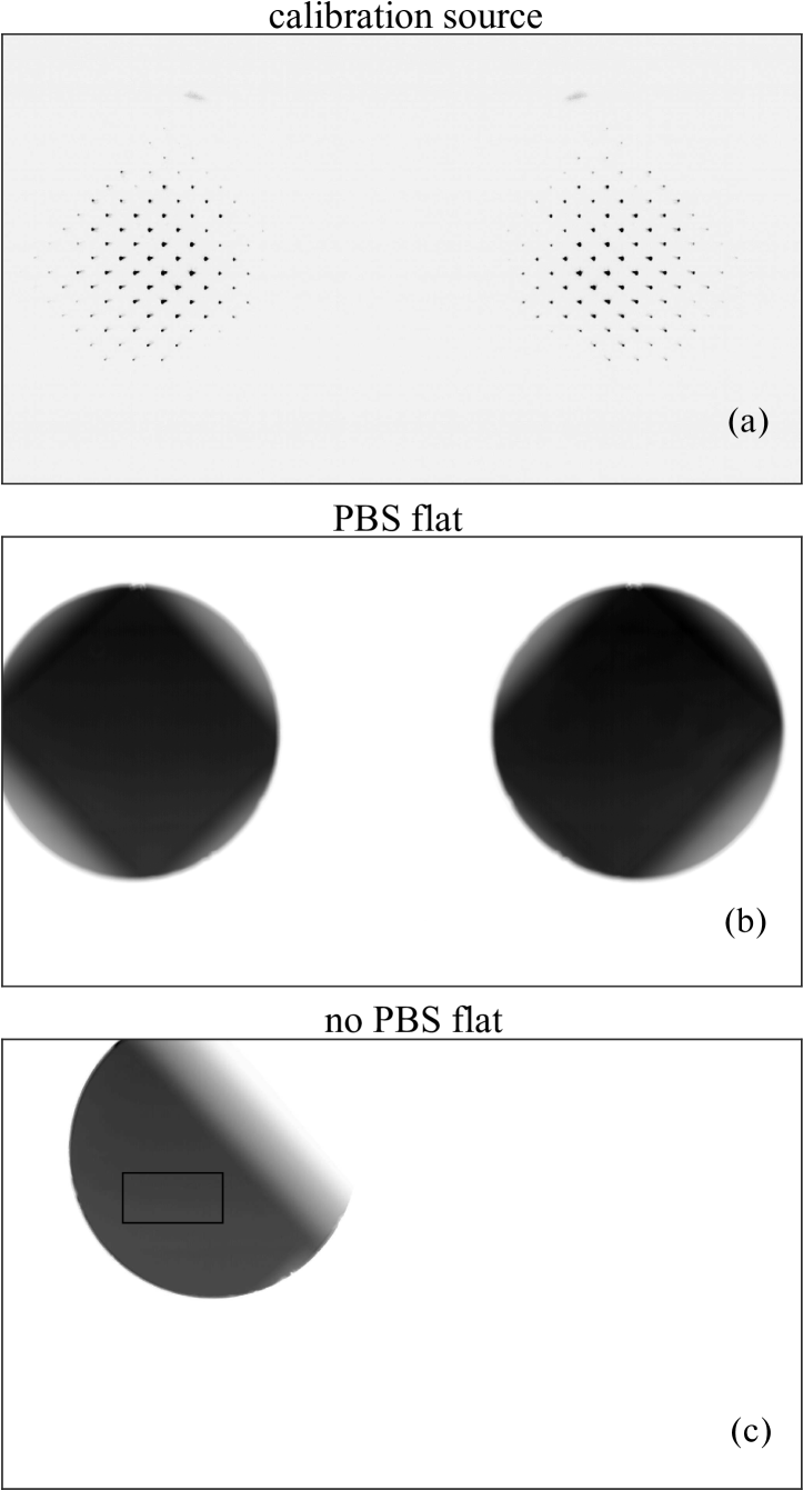
Figure 5: Image examples: (a)—a calibration source; (b)—a flat field frame when operating with the Polarizing Beamsplitter Cube—PBS; (c)—a flat field frame when operating without the PBS (speckle interferometry mode). The black rectangle on the panel shows the detector area $512\times 256$ px, which is read in the speckle interferometry mode.

The prefocal unit also contains a linear polarizer that can be inserted into the beam to calibrate the angle of rotation of the half-wave plate. The relay mirrors of the auxiliary detector, the calibration source, and the linear polarizer are located on the Standa 8MT173-30 linear translator (stepper motor + ball guide).

An important element of the prefocal unit is the field aperture, which is a hole with a diameter of 3.5 mm, which corresponds to $35^{\prime\prime}$ on the celestial sphere. The field aperture is permanently set. Note that not the entire field of view cut out by the field stop is non-vignetted, this issue is discussed below in Section 2.3.

2.2 Collimated beam unit

From the main focal plane begins the main part of the optics of the instrument, the main purpose of which is the formation of images with specified characteristics on the detector. The key elements in the optical design are the collimator, which forms a collimated beam, and the lens, which focuses this beam on the detector. The focal lengths of the collimator and objective are 38.1 and 88.9  mm, respectively. The scheme provides a final magnification of $2.33\times$, which corresponds to a scale of $20.33$ mas/px for the main detector pixel size of 4.6 $\mu$m. This magnification ensures optimal sampling of the focal plane at wavelengths of 493 nm and more, which is a necessary condition for the implementation of speckle interferometry. The exact value of the scale and rotation angle of the detector is determined by observing binary stars for which the coordinates of the components are known from Gaia DR3 (Gaia Collaboration et al., 2022).

Behind the collimator in the plane of the exit pupil in the Standa 8MRU-1 rotation drive, a Thorlabs SAHWP05M-700 half-wave plate is installed, which acts as a modulator in the polarimetry mode. The half-wave plate is driven by a stepper motor through a belt drive (Standa 8MRU).

Behind the half-wave plate there is an atmospheric dispersion compensator, which consists of two direct vision prisms installed in independently rotating Standa 8MR151 drives (stepper motor + worm gear). Each prism, in turn, consists of two prisms made of LZOS F1 and LZOS K8 glass, with wedge angles $15\,.\!\!^{\circ}9$ and $18\,.\!\!^{\circ}65$, respectively. The aperture of the prisms is $15\times 15$ mm. The prisms are manufactured by RIVoptics.

These prisms have been used by us since mid-2018. Previously, we used prisms with much larger wedge angles, which resulted in a significant distortion. The prisms in operation nowadays have a distortion of 0.72%, it is corrected during processing.

During observations, the rotation angles of the prisms are chosen so that the total dispersion introduced by them is equal in absolute value, and opposite in direction—to atmospheric dispersion (Safonov et al., 2017). Atmospheric dispersion is calculated using the formulas from Owens (1967), based on the current parameters of the atmosphere: pressure, temperature, humidity, which are measured by a weather station. The available prisms in the current configuration make it possible to compensate for atmospheric dispersion at altitudes above $28^{\circ}$ (the most critical band is 880 nm).

A 12-position filter wheel is installed after the prisms of the atmospheric dispersion compensator. It is controlled by a Standa 8MR174 rotation drive (stepper motor + worm gear). Currently, 7 filters are used: $V$, $R_{c}$, $I_{c}$, mid-band filters centered at wavelengths of 550, 625, 880 nm, with half-widths of 50, 50, and 80 nm, respectively. An H$\alpha$ filter with a half-width of 8 nm is also installed. The filter bandwidths are shown in Fig. 1.

2.3 Camera unit

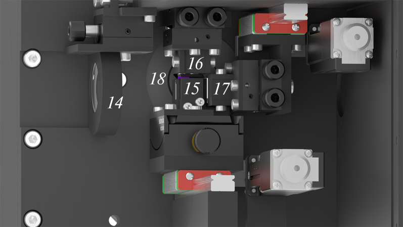
Figure 6: The camera unit (render of CAD model). The designations are the same as in Fig. 2.

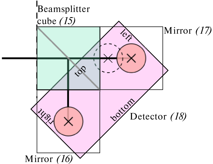
Figure 7: Scheme of image formation on the detector (shown in pink), view from the side of the detector, to scale. The red circles outlined by solid lines are the field of view in the polarimetry mode, the circle with a dashed line is the field of view in the speckle interferometry mode (the PBS presented by the green square is removed from the beam). The edges of the frame are also signed: left, right, bottom and top.

Before 2022 we used a Wollaston prism as a beam-splitting element. Although the prism has some advantages, such as simplicity of design and polarimeter alignment, it also has significant drawbacks. First of all, this is dispersion, which arises due to the dependence of the difference between the refractive indices $n_{o}$ and $n_{e}$ on the wavelength. The dispersion smears the images along the beam separation line, which reduces the $S/N$ ratio in the image spectrum. We quantify this effect in Section 4.3. The second feature of the Wollaston prism is that it introduces differential distortion into images. One of the images is compressed and the other one is stretched by 1.5% in the direction connecting the images.

In the new design of the instrument, we tried to use a larger number of detector pixels to realize a larger field of view. However, this would require an increase in the beam separation angle. Since the dispersion of the Wollaston prism is proportional to its average separation angle, the dispersion would reach an unacceptably high level. In this regard, we abandoned the Wollaston prism in favor of a Polarizing Beamsplitter Cube (PBS, (15) in Figs. 2 and 6). The PBS reflects light polarized in a plane perpendicular to the plane of incidence, while light polarized along the plane of incidence is transmitted. The PBSs lack dispersion.

The PBSs are most effectively implemented using dichroic coatings, however, in this case, the working spectral band is not very wide. There is no commercially available PBS that would operate in the entire wavelength range that we are interested in. Therefore, we use two PBSs, the first one is for 390 to 730 nm and the other—for 660 to 1160 nm. The cubes can be swapped using a motorized translator based on the Standa 8CMA06-25/15 actuator.

The beam reflected by PBS propagates at an angle of $90^{\circ}$ to the optical axis and to the beam that has passed through the PBS. Thus, to focus both beams on the detector, additional mirrors (16) and (17) are required (see Figs 2, 6 and 7). These mirrors are tilt-adjustable. The mirror (17), which reflects the transmitted beam, is mounted on a motorized translator based on a Standa 8CMA06-25/15 actuator. Movement is performed towards to/away from the detector. This ensures accurate relative focusing of images. The detector itself is oriented at an angle of $45^{\circ}$ to the main optical axis (before the PBS), which facilitates the placement of images corresponding to horizontal and vertical polarizations on it. The scheme for relaying images to the detector is shown in Fig. 7.

In the mode of speckle interferometry, which is the subject of this paper, the PBS is removed from the beam, so that all light passes to the mirror (17). In this case, the mirror itself shifts to the detector by 2.5 mm, eliminating the need to refocus the telescope. Note that the center of the field of view shifts along the detector, see Figs 5 and 7. A large field of view is used to center the object, and in standard observations, an area of $512\times 256$ px is read, which corresponds to $10\,.\!\!^{\prime\prime}4\times 5\,.\!\!^{\prime\prime}2$ (see Section 2.5 below).

2.4 Detector characteristics

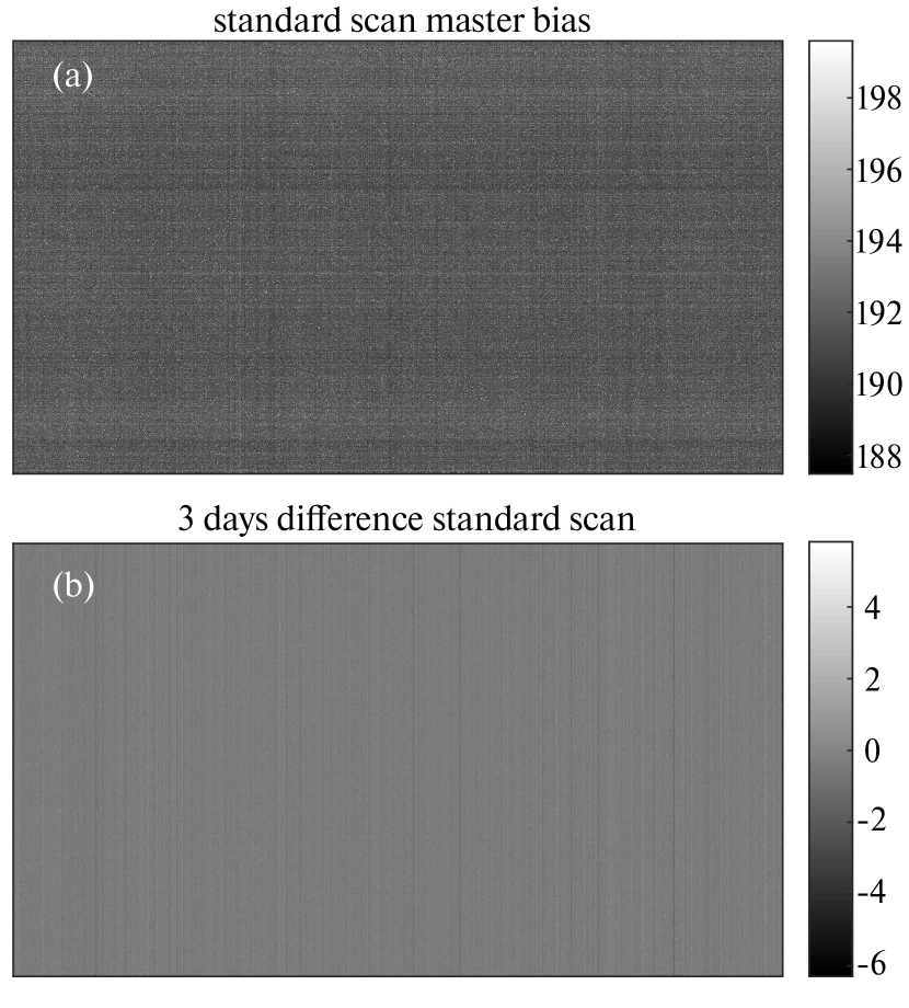
Figure 8: (a)—example of master bias; (b)—the difference between two master biases taken with an interval of 3 days. The width of the range of displayed values is the same. The master bias was calculated over 500 frames, while discarding 1% of the brightest and 1% of the dimmest values of each pixel in the series.

Knowledge of the characteristics of the main detector is of great importance for evaluating the efficiency of the instrument in solving astrophysical problems, for determining the optimal operating mode of the instrument, and also for developing processing methods. In this subsection, we present the results of measuring the main characteristics of the Hamamatsu ORCA-quest detector when operating without illumination and with uniform illumination. The Hamamatsu ORCA-quest detector can operate in two modes: standard and ultra-quiet, which differ in readout speed and readout noise. The mode parameters are shown in Table 1. The study of the detector was carried out by us in both modes.

In CMOS detectors, as in CCDs, some constant number is added to the signal, which is called bias. The bias value is fairly constant, but there is a slight dependence on the position in the frame and on time. To analyze bias stability, we obtained several series of frames without illumination. For each series, the per-pixel median (master bias) was calculated, an example can be seen in Fig. 8. For series taken with an interval of 3 days, the bias difference turned out to be less than 0.1 ADU, so the bias drift at shorter times can be neglected.

An analysis of the dependence of the bias type on the registration parameters showed that the following parameters should be the same for scientific frames and for bias frames used for their reduction: the size and position of the read area, binning, standard/ultra-quiet detector operation mode, and exposure. The effect of exposure dependence of bias is especially noticeable when observing faint sources in the ultra-quiet mode.

The bias frames show the vertical and horizontal structure (see Fig. 8). This structure has a random component, that is, its realization changes from frame to frame. Because of this, it appears as an increase in the level of the power spectrum at frequencies $|f_{x}|\approx 0$ or $|f_{y}|\approx 0$. The method of elimination of this effect in speckle interferometric processing is presented in Section 3.1.

Based on the series of bias frames, we estimated the root mean square of per-pixel standard deviations (not taking into account outliers beyond the second and 98th percentiles) $\sigma_{\mathrm{RON}}$, it turned out to be equal to 0.241 and 0.422 $e^{-}$, for ultra-quiet and standard modes, respectively, which is consistent with the specifications, Table 1. Figure 9 shows the bias sample distributions normalized to the RMSD of the readout noise (the normalization was performed individually for each pixel). Also, for comparison, the standard normal distribution is given, as one can see, it describes well the distributions of samples up to the values $3\sigma_{\mathrm{RON}}$. At large normalized deviations, a significant excess of the measured histogram begins in comparison with the standard normal distribution. Note that a similar effect is observed in EMCCD, it is caused by the contribution of spurious charge (CIC noise) Harpsøe et al. (2012). As can be seen, the readout noise distribution of the Hamamatsu ORCA-quest detector is much more ‘‘normal’’ than that of the Andor iXon 897 EMCCD. In the simulations in Section 4, we will assume the readout noise is normal, with the RMSD corresponding to the measurements made.

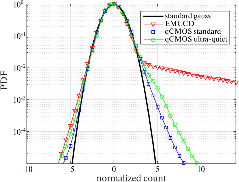
Figure 9: Distribution of the deviation of bias from the mean (the deviation is normalized to the RMSD of the readout noise). The blue line with squares is the CMOS standard mode, the green line with circles is the CMOS ultra-quiet mode, the red line with triangles is EMCCD Andor iXon 897 operating at $G_{\mathrm{EM}}=500$. The solid thick line is the standard normal distribution.

The dark current measured by us at a detector temperature of $-20^{\circ}$C (air cooling) turned out to be 0.011 and 0.013 $e^{-}$/px/s for the ultra-quiet and standard modes, respectively. For typical exposures that we use, the level of dark current is negligible.

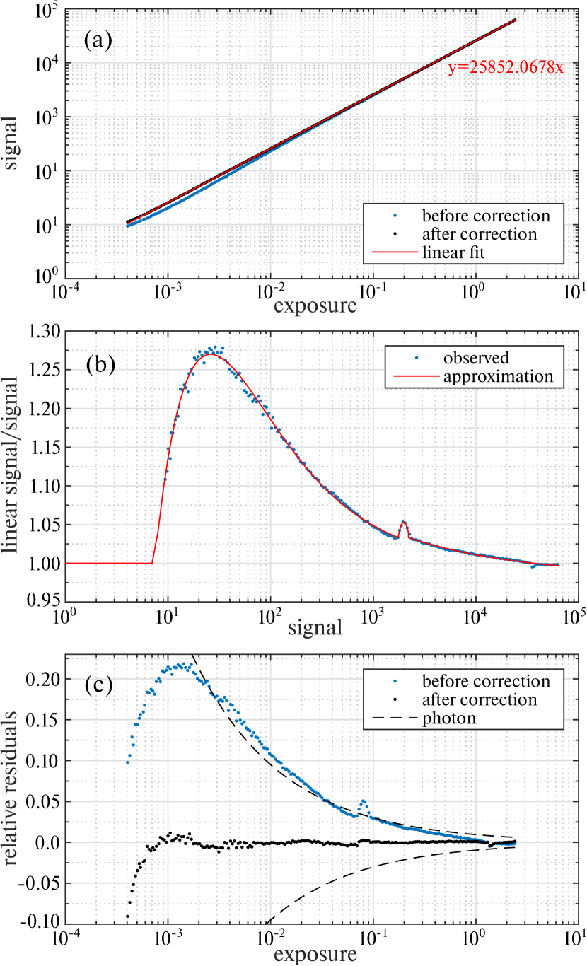
Figure 10: (a)—dependence of signal on exposure before and after non-linearity correction, (b)—function approximating dependence ‘‘ratio of linear approximation of signal to signal – signal’’, (c)—comparison of relative deviations from the linear approximation of the dependence of the signal on the exposure for data with and without nonlinearity correction, the dashed line reflects the RMSD value of photon noise in a pixel.

To study the nonlinearity of the detector response, we used a stabilized light source (halogen lamp). The average signal was 25 000 ADU/s. Frames were obtained in the standard mode with exposures $t$ from 0.4 ms to 2.4 s on a uniform logarithmic grid, which corresponds to signal range from 10 ADU to 60 000 ADU (covers the entire ADC range). The constant bias structure was eliminated by subtracting the master bias. Then we performed photometry over an area of $128\times 128$ px (relative illumination variations over the area under consideration were about 1%).

Figure 10a shows the dependence of the average signal $s$ on the exposure time. We have approximated the dependence $s(t)$ by the $at$ function, the relative deviation $\Delta s=(at-s(t))/at$ is shown in the same figure below. As can be seen, $\Delta s$ increases towards the region of weak signals and reaches 0.2, which indicates a significant nonlinearity of the detector. In addition, the deviation curve has a complex shape with a jump in the 2000 ADU signal region, which is probably caused by the junction of the ranges of the two ADCs.

We have approximated the quantity $r(s)=at/s(t)$ by a function of a special form; we will denote this approximation as $r^{\prime}(s)$. The approximation is illustrated in Fig. 10b. To correct the nonlinearity, the signal, after subtraction for bias, was multiplied by $r^{\prime}(s)$. The accuracy of the correction was checked over the region $512\times 512$ px. It is better than 1% for a signal greater than 100 ADU. For signals from 10 to 100 ADU, the accuracy is about 2%. For the ultra-quiet mode, the dependence was obtained in a similar way. When performing classic long-exposure photometric measurements with this detector, special attention must be paid to non-linearity correction.

2.5 Choice of readout parameters

When observing, we must choose the optimal readout parameters for the detector: its mode (standard/ultra-quiet), field of view, exposure time.

First, the size of the read area must be minimized in order to ensure fast reading, which is especially relevant for ultra-quiet operation. However, in standard mode, fast reading is preferred as well as we use short exposures to prevent saturation.

It follows from previous experience with speckle interferometric observations that a field of view of $5^{\prime\prime}\times 5^{\prime\prime}$, or $256\times 256$ px, is large enough. Increasing the width of the field of view does not affect the reading speed, but allows a more reliable estimate of the background. As a result, we chose the rectangular field $512\times 256$ px ($10^{\prime\prime}\times 5^{\prime\prime}$) as the default field of view for the speckle interferometry mode, see Fig. 5c. Such a region can be read in 0.96 ms and 22.98 ms in standard and ultra-quiet modes, respectively.

The Hamamatsu ORCA-quest detector has a rolling shutter mode and a global exposure start mode, there is no global shutter mode. We use only rolling shutter mode, so the rows are read in turn, which ensures minimal gaps between exposures. For standard readout there is an electrical shutter mode to obtain exposures shorter than 1 frame readout time. But there is no such possibility in ultra-quiet mode. The rolling shutter can make it difficult to achieve the isoplanatism conditions necessary for the implementation of speckle interferometry, we discuss this issue in Appendix A.

The total vignetted field of view reaches $35^{\prime\prime}$ in diameter (see Fig. 5) and is used by us to center the object.

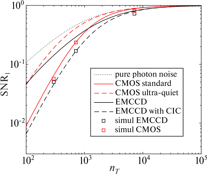
Figure 11: Dependence of the $S/N$ ratio in the power spectrum per one frame on the average number of photons per frame. The dotted line—no read noise and no CIC noise. The red solid and dashed lines—CMOS Hamamatsu ORCA–quest for standard and ultra-quiet modes, respectively. The black solid and dashed lines—EMCCD Andor iXon 897 without and with spurious charge (CIC noise), respectively. The black and red squares show the numerical simulation data from Section 4.3 for EMCCD and CMOS, respectively.

To choose the operating mode: standard/ultra-quiet, we consider the contributions of photon noise and readout noise to the S/N ratio when estimating the average power spectrum (Miller, 1977):

$$\mathrm{SNR}_{1}(\bm{f})\!\!\!\! \!\!\!\!=\bigg{(}1+\Big{(}n_{T}\langle|I_{N}(\bm{f})|^{2}\rangle\Big{)}^{-1}+$$ (1)

$$\dfrac{N_{\mathrm{pix}}p_{\mathrm{CIC}}}{n_{T}^{2}\langle|I_{N}(\bm{f})|^{2}\rangle}+\dfrac{N_{\mathrm{pix}}\sigma^{2}_{\mathrm{RON}}}{n_{T}^{2}\langle|I_{N}(\bm{f})|^{2}\rangle}\bigg{)}^{-1},$$

where $\bm{f}$ is the spatial frequency vector, $n_{T}$ is the average number of photons per frame, $N_{\mathrm{pix}}$ is the number of pixels used to calculate the power spectrum, $p_{\mathrm{CIC}}$ is the probability of registering a CIC electron in a pixel, $\sigma_{\mathrm{RON}}^{2}$ is the dispersion of readout noise, $\langle|I_{N}(\bm{f})|^{2}\rangle$ is the average signal in the absence of photon and readout noise, normalized so that $\langle|I_{N}(0)|^{2}\rangle=1$. Expression (1) is written per 1 frame. In it, the first term (equal to one) is responsible for atmospheric noise, the second—for photon noise, the third—for CIC noise, and the fourth—for readout noise. In the case of CMOS, we assume that there is no CIC noise.

For the quantity $\langle|I_{N}(\bm{f})|^{2}\rangle$ at frequencies $|\bm{f}|>r_{0}/\lambda$ the generally accepted model is as follows:

$$\langle|I_{N}(\bm{f})|^{2}\rangle=0.435\Bigg{(}\dfrac{r_{0}}{D}\Bigg{)}^{2}\widetilde{T_{0}}(\bm{f})|\widetilde{O}(\bm{f})|^{2},$$ (2)

where $r_{0}/D$ is the ratio of the Fried radius to the aperture diameter, $\widetilde{T_{0}}(\bm{f})$ is the diffractive aperture OTF, $|\widetilde{O}|^{2}$ is the object visibility function module. For typical observation conditions with a 2.5-m telescope ($r_{0}\!=\!0.1$ m and a point-like object) $\langle|I_{N}(f)|^{2}\rangle\!=\!2.7\!\times\!10^{-4}$ at $f=0.5D/\lambda$ (see Fig. 20).

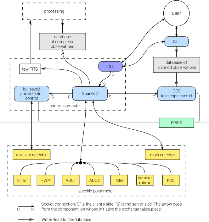
Figure 12: Scheme of the hardware-software complex of the instrument.

Figure 11 shows the dependences of $\mathrm{SNR}_{1}$ on $n_{T}$ for the size of the image spectrum calculation area $140\times 140$ px, seeing $0\,.\!\!^{\prime\prime}73$, in the band $I_{c}$. The evaluation was carried out for CMOS (standard and ultra-quiet modes), as well as for EMCCD with and without taking into account CIC noise.

As can be seen, the EMCCD detector would have an advantage over CMOS in the region of low fluxes ($n_{T}<10^{3}$ photons/frame) if it were not subject to the effect of CIC noise. Accounting for realistic CIC noise $p_{\mathrm{CIC}}=0.045$ eliminates the advantage of EMCCD. Previously, Tokovinin et al. (2010) noted that CIC noise is the limiting factor in speckle interferometric observations of faint objects with EMCCD.

It can also be seen from Fig. 11 that it is more beneficial for CMOS to use the ‘‘ultra-quiet’’ readout mode if the flux is less than $10^{4}$ photons/frame. At higher fluxes, the difference becomes negligible and the standard mode becomes preferrable due to the fact that it allows faster reading. Starting from about $n_{T}=2.4\times 10^{5}$ photons/frame, the signal in the brightest pixel approaches saturation. To prevent loss of information due to saturation, we decrease the exposure. Exposure reduction while maintaining 100% time efficiency is possible up to 0.96 ms. Exposure reduction is also useful in suppressing the effects of speckle smearing due to temporal evolution and telescope mount vibration.

2.6 Control software

The control software consists of the following main components (diagram in Fig. 12):

• The main control program Sparkle2 (implementation in C++) interacts with the motorization drives (7 pcs.), as well as the main detector. Sparkle2 performs recording of the raw data (see below).

• The control program of the auxiliary detector bullseye2 (implementation in C++). Provides object centering.

• The user interface Specktate (implementation in PyQt5) is intended for convenient management of routine measurements.

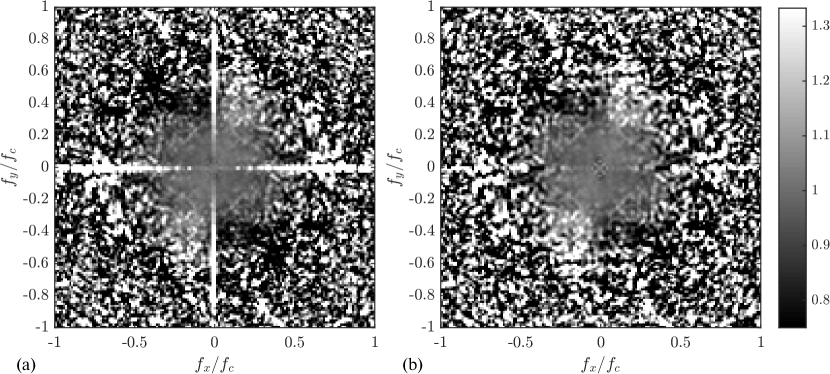
Figure 13: Comparison of power spectra normalized by themselves azimuthally averaged without and with the procedure for removing the cross artifact.

The programs Sparkle2 and bullseye2 are constantly running on the control computer ‘‘in the background’’, interaction with them is carried out via a TCP/IP socket using commands that make up a special protocol. The user can issue commands directly over the socket connection; in this case, maximum control flexibility is achieved (engineering mode). An alternative way is to control via a Specktate GUI running locally on the user’s PC. Specktate communicates with Sparkle2 over the same socket connection used in engineering mode. Specktate provides a high degree of automation for routine observations.

Interaction with the telescope control program is performed via the EPICS connection. Sparkle2 automatically requests the coordinates of the object, meteorological parameters (temperature, pressure, humidity) necessary for the correct operation of the atmospheric dispersion compensator. This information is written to the metadata of the FITS file.

Sparkle2 provides automatic object tracking (‘‘autoguiding’’) by determining the current position of the object in the frame and giving the telescope the corrections necessary to keep the object in the center of the field of view. Due to the fact that the main detector registers frames at a sufficiently high frequency (10–100 frames per second), autoguiding is performed using the image coming from it during the registration of scientific data.

The series received with the main detector are written to FITS files. The metadata is also used to populate the observational database sppdata for subsequent processing. Information about planned observations is stored in the sai2p5 database, which has a uniform structure for all instruments of the 2.5-m telescope. The sai2p5 database contains information about the coordinates of objects, time constraints on observations, links with observations of other objects, optimal environmental conditions (seeing, sky background, atmospheric transparency), and also about the mode in which the instrument should operate.

3 PROCESSING

Atmospheric turbulence distorts the wavefront coming from a distant source, resulting in blurry images. The half-width of a long-exposure star image—seeing—is on the order of $1^{\prime\prime}$. For binary stars with a separation between the components that is less than the seeing, estimating the binarity parameters: separation, position angle, flux ratio from a long-exposure image—is difficult or impossible at all due to the influence of photon noise and detector noise.

However, the binarity parameters can be extracted from short-exposure images of the star by applying the speckle interferometry method. Classical speckle interferometry is based on the estimation of the average power spectrum from a series of short-exposure images of an object and its subsequent approximation by a model, in this case, of a binary source. In this Section, we describe the processing of data obtained with a speckle polarimeter using the speckle interferometry method.

3.1 Reduction, approximation and error estimation

The preliminary reduction of each frame consists of the following steps.

• First, the master bias is subtracted from the frame. It is calculated from a series of 1000 frames obtained on the same observational night.

• For areas of the frame outside the window with the object under study, the average background value is estimated and subtracted from the entire frame.

• The image of the object is centered in the window. To estimate the required offset, a Gaussian filter is applied to the image to reduce the effect of noise.

• The ORCA C15550-20UP detector exhibits an artifact in the form of a cross in the averaged power spectrum (see Fig. 13a). We remove this artifact in the following way. The horizontal and vertical structure of the image is estimated from a number of rows and columns outside the scientific data window. This structure is subtracted from the data in the window. This operation allows one to even the vertical and horizontal components of the cross on the future power spectrum. After that, the image power spectrum is calculated, the vertical and horizontal components of the cross behind the cutoff frequency $D/\lambda$ are estimated and subtracted from it, see the result in Fig. 13b.

• Next, the frame power spectrum is corrected for the distortion of the ADC and the Wollaston prism (if it is the beam-splitting element). The power spectrum is rotated to the angle corresponding to the central moment of the series.

• Further, the photon bias is subtracted from the already averaged power spectrum. We estimate it by the values of the power spectrum beyond the cutoff frequency.

After obtaining the averaged power spectrum, it is approximated by a model function.

As is known, the image $I$ is a convolution of the intensity distribution $O$ and the point spread function $T$. For the Fourier spectrum $\widetilde{I}$ of an instantaneous image one can write:

$$\widetilde{I}(\bm{f})=\widetilde{O}(\bm{f})\widetilde{T}(\bm{f}),$$ (3)

where $\bm{f}$ is the spatial frequency vector, $\widetilde{O}$ is the object visibility, $\widetilde{T}$ is the optical transfer function (OTF). The OTF is defined as:

$$\widetilde{T}(\bm{f})\!=\!\!\int_{W}\!\!\!W(\bm{x})W^{*}(\bm{x}+\lambda\bm{f}){e}^{(i\phi(\bm{x})-i\phi(\bm{x}+\lambda\bm{f}))}d\bm{x},$$ (4)

where integration is performed in the pupil plane, $\bm{x}$ is the pupil plane coordinate, $W$ is the pupil function equal to one inside the aperture and zero outside, $\phi$ is the instantaneous phase distribution in the pupil. As can be seen, equation (3) takes into account diffraction at the edges of the aperture, telescope aberrations, and atmospheric distortions.

Fourier spectrum modulus is squared and averaged over the entire series of short-exposure images:

$$\langle{|\widetilde{I}(\bm{f})|}^{2}\rangle={|\widetilde{O}(\bm{f})|}^{2}\langle{|\widetilde{T}(\bm{f})|}^{2}\rangle.$$ (5)

To estimate the square of the visibility amplitude, it is necessary to know the value $\langle{|\widetilde{I}_{\rm ref}|}^{2}\rangle$, which can be obtained from the observation of a single star (for a point object $\widetilde{O}_{\rm ref}=1$) carried out, if possible, either shortly before or shortly after the observation of the scientific object:

$${|\widetilde{O}|}^{2}\approx\dfrac{\langle{|\widetilde{I}(\bm{f})|}^{2}\rangle}{\langle{|\widetilde{I}_{\rm ref}(\bm{f})|}^{2}\rangle}.$$ (6)

In the vast majority of cases, to obtain $\langle{|\widetilde{I}_{\rm ref}|}^{2}\rangle$, instead of observing a close reference single star, one can use an azimuthally averaged initial power spectrum $\langle{|\widetilde{I}|}^{2}\rangle$.

Let us find the square of the modulus of visibility under the assumption that the object consists of two point–like sources. The intensity distribution in this case is

$$O^{0}(\alpha_{x},\alpha_{y})=\delta(\alpha_{x},\alpha_{y})+\epsilon\,\delta(\alpha_{x}-\Delta_{x},\alpha_{y}-\Delta_{y}),$$ (7)

where $\delta$ is the delta function, $\epsilon$ is the ratio of component fluxes, $\Delta_{x},\Delta_{y}$ is the separation, $\alpha_{x},\alpha_{y}$ are the angular coordinates. The use of the delta function to model a star is justified because most stars have angular sizes much smaller than the diffraction limited resolution of the 2.5-m telescope. The Fourier transform of the given intensity distribution is:

$$\widetilde{O^{0}}\left(f_{x},f_{y}\right)=\sqrt{A_{1}}\left(1+\epsilon\,e^{\left(-i2\pi(f_{x}\Delta_{x}+f_{y}\Delta_{y})\right)}\right)\!,$$ (8)

where $A_{1}=(1+\epsilon)^{-2}$ is the normalization factor. Then, taking the modulus and squaring it, we have:

$${|\widetilde{O^{0}}\!\left(f_{x},\!f_{y}\right)\!|}^{2}\!\!\!=\!A_{1}\!\left(1\!+\!\epsilon^{2}\!\!+\!2\epsilon\!\cos{\left(2\pi(f_{x}\Delta_{x}\!\!+\!\!f_{y}\Delta_{y})\right)}\right)\!.$$ (9)

To obtain the binarity parameters, we approximate the root of the power spectrum normalized by its azimuthal average. The applied model for approximation is the following:

$$\begin{array}[]{l}|\widetilde{O^{0}}\left(f_{x},f_{y}\right)\!|\!=\!\Bigl{|}\sqrt{A_{1}}\bigl{(}1+\epsilon e^{\left(-i2\pi(f_{x}\Delta_{x}+f_{y}\Delta_{y}+\phi)\right)}\bigr{)}\times\\[5.0pt] \left(1+\sqrt{f_{x}^{2}+f_{y}^{2}}A_{a}\cos{2(\theta_{a}-\theta_{a_{\rm ref}})}\right)\Bigr{|},\\[-5.0pt] \end{array}\\$$ (10)

where $A_{1}=(1+\epsilon)^{-2}$ is the normalization factor, $\epsilon$ is the ratio of component fluxes, $\Delta_{x},\Delta_{y}$ is the separation. Compared to (8), additional parameters have been added to the expression: $\theta_{a_{\rm ref}}={\arctan^{2}}(f_{y},f_{x})$, $A_{a}$ and $\theta_{a}$ are the parameters characterizing the amplitude and angle of the asymmetric component, respectively, which must be taken into account due to the jitter of the telescope. The parameter $\phi$ is the shift of the power spectrum relative to the central maximum in the direction perpendicular to the fringes. It should be noted that the model function is also normalized by its azimuthal average, similarly to how it is done with the estimation of the root of the power spectrum. An example of approximation is shown in Fig. 14.

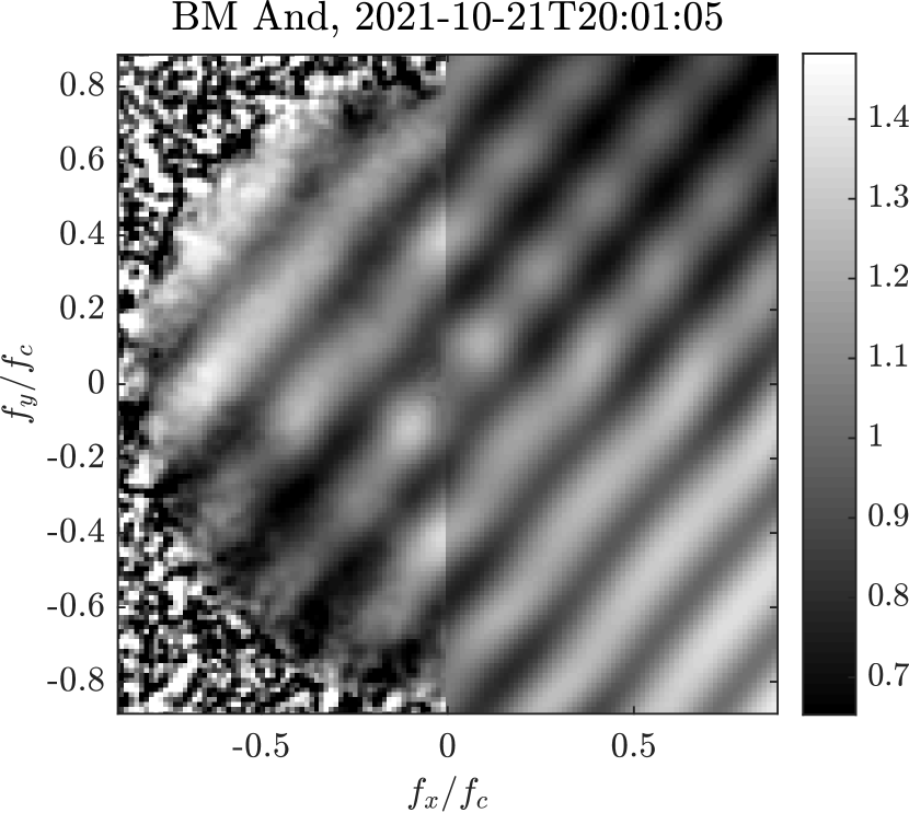
Figure 14: An example of power spectrum approximation. The left half is the average power spectrum normalized by its azimuth mean, the right half is the binary source model. Note that the power spectrum has central symmetry, so the half-plane contains all the useful information.

The error of the binarity parameters is estimated by the ‘‘bootstrap’’ method (Efron & Tibshirani, 1993). The sample of indices used to average the frame power spectrum is repeatedly randomly generated. In this case, the length of this sample is equal to the length of the original series, and the set of frames used is different. So, as a result of such a sample generation, the same frame can be counted several times, while the other—never. We generate twenty such index samples. Using these indices, we average the power spectra. As a result, we have 20 averaged power spectra for one series. We then do exactly the same processing for each of the 20 power spectra. And, further, we approximate each of them by the function described above. This results in a sample of 20 sets of binarity parameter values. For this sample, we estimate the standard deviation of each parameter.

3.2 Estimation of the achievable contrast curve

In those cases where no binarity has been found in the star, the important information that we can glean from observation can be an estimate of the achievable contrast curve $\epsilon_{\rm lim}(\rho)$. The curve of achievable contrast characterizes the minimum possible registrable ratio of component fluxes for a given observation depending on the angular distance. In other words, the component (if it exists) at the angular distance $\rho$ with the flux ratio $\epsilon$ greater than $\epsilon_{\rm lim}(\rho)$ will be unambiguously registered by us.

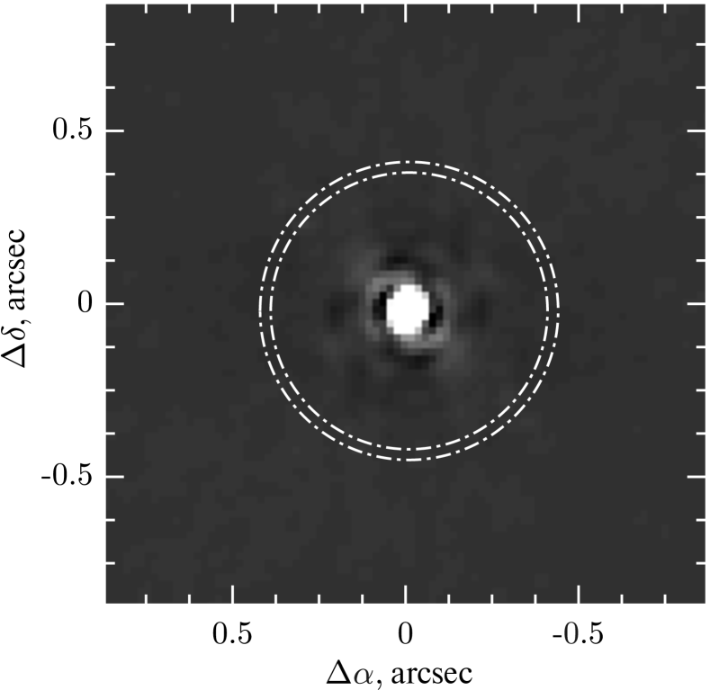
Figure 15: ACF example. The dashed-dotted ring shows the area in which the RMSD is calculated for the estimate $\epsilon_{\rm lim}$, in this case, $\epsilon_{\rm lim_{0.4}}$.

Let us obtain the formula for determining $\epsilon$ for each point of the autocorrelation function (ACF, see Fig. 15). To do this, we take the inverse Fourier transform of the resulting function ${|\widetilde{O^{0}}\left(f_{x},f_{y}\right)|}^{2}$ (9):

$$\begin{array}[]{l}\Psi\left(\alpha_{x},\alpha_{y}\right)=A_{2}A_{1}\big{(}(1+\epsilon^{2})\delta(\alpha_{x},\alpha_{y})\,+\\[7.0pt] \epsilon\delta(\alpha_{x}\!-\!\Delta_{x},\alpha_{y}\!-\!\Delta_{y})+\epsilon\delta(\alpha_{x}\!+\!\Delta_{x},\alpha_{y}\!+\!\Delta_{y})\big{)}.\end{array}$$ (11)

Next, we note that, by definition, $\Psi(0,0)=~{}1$. Therefore, $A_{2}A_{1}(1+\epsilon^{2})=1$. That is, $A_{2}=(1+\epsilon)^{2}/(1+\epsilon^{2}$).

Finally we get:

$$\Psi\left(\alpha_{x},\alpha_{y}\right)=\delta(\alpha_{x},\alpha_{y})\,+$$ (12)

$$\;\;\dfrac{\epsilon}{1+\epsilon^{2}}\,\delta(\alpha_{x}-\Delta_{x},\alpha_{y}-\Delta_{y})+$$

$$\;\;\dfrac{\epsilon}{1+\epsilon^{2}}\,\delta(\alpha_{x}+\Delta_{x},\alpha_{y}+\Delta_{y}).$$

This shows that the ratio of the fluxes of the binary components can be obtained from the ratio of the intensities of the secondary and central peaks in the ACF.

Now let us take a real ACF obtained from observations. Due to factors introduced by the atmosphere, instrument and method, we have some noise in the resulting ACF.

Our task is to find the dependence of the achievable contrast (flux ratio) on the distance to the central star. Let us move from the Cartesian coordinate system $\alpha_{x},\alpha_{y}$ to the polar one $\rho,\varphi$. Let us denote the intensity of some ACF point as $\eta$. Moreover, as unity we take the value of the coefficient of the Gaussian approximating the central peak, plus the bias. Let us find for each ring with radius $\rho$ the value of reachable $\eta_{\rm lim}$ by the formula:

$$\eta_{\rm lim}(\rho)=5\sigma(\rho)+\overline{\eta(\rho,\varphi)},$$ (13)

where

$$\sigma(\rho)=\sqrt{\dfrac{1}{n-1}\sum_{\varphi}\left(\eta(\rho,\varphi)-\overline{\eta(\rho,\varphi)}\right)^{2}}.$$ (14)

The line $\overline{\phantom{15}}$ means averaging over the angle in the ring, $n$ is the number of pixels in the ring. The summation over $\varphi$ in the expression for the standard deviation $\sigma$ means the summation over the pixels in the ring.

Using the equation (12), we have:

$$\dfrac{\epsilon_{\rm lim}}{1+{\epsilon_{\rm lim}}^{2}}=\eta_{\rm lim}.$$ (15)

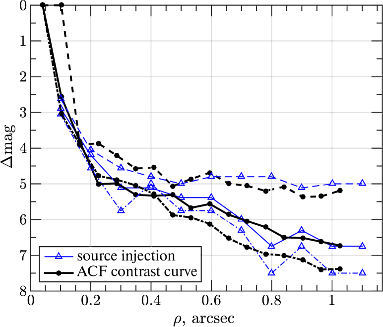
Figure 16: Comparison of achievable contrast curves, obtained from ACF and by source injection. Lines of different types correspond to observations of different stars.

From here we get:

$$\epsilon_{\rm lim}(\rho)=\dfrac{1-\sqrt{1-4{\eta_{\rm lim}}^{2}(\rho)}}{2\eta_{\rm lim}(\rho)}.$$ (16)

Now, based on this dependence, we can argue that given star has no components with contrast $\epsilon>\epsilon_{\rm lim}(\rho)$ at an angular distance $\rho$.

It is possible to verify the achievable contrast curve by adding a secondary component with known parameters to the real data. We multiply the power spectrum of a single star directly by expression (9) in accordance with expression (5), where we vary the separation and for each separation find the minimum (in terms of flux ratio) contrast value at which the ‘‘artificial’’ injected source is still detected at the ACF. The comparison illustrated in Fig. 16 shows that the contrast curve from the ACF method is estimated adequately.

4 DIRECT MODEL OF SPECKLE INTERFEROMETRIC OBSERVATIONS

To study the capabilities of the detector and verify the processing methods, we created a program that allows us to generate images recorded by the detector in the focal plane of the instrument. The model takes into account wavefront distortions in a turbulent atmosphere, in an optical system, as well as photon noise and detector noise.

The von Kármán turbulent disturbance model gives the following expression for the phase distortion power spectrum (see Johansson & Gavel (1994); Xiang (2014)):

$$\widetilde{P}(f_{x},f_{y})\!=\!\dfrac{4\pi^{2}}{G_{x}{G_{y}}}0.00058\,r_{0}^{-5/3}\!\left(f_{x}^{2}\!+\!f_{y}^{2}\!+\!\dfrac{1}{L_{0}}\right)^{\!\!-11/6}\!\!\!,\\$$ (17)

where $f_{x},f_{y}$ are the spatial frequencies, $G_{x},G_{y}$ are the phase screen dimensions (in meters), $L_{0}$ is the outer scale of turbulence , $r_{0}$ is the Fried radius related to the turbulence profile $C_{n}^{2}(h)$ as follows:

$$r_{0}=\left(0.423\left(\dfrac{2\pi}{\lambda}\right)^{2}\mathrm{sec}\gamma\int_{0}^{H_{\rm max}}C_{n}^{2}(h)dh\right)^{-3/5},$$ (18)

where $\lambda$ is the wavelength, $\gamma$ is the zenith angle, $h$ is the altitude. The integration is carried out from the altitude of the telescope to some maximum turbulence altitude $H_{\rm max}$.

We will model the phase screen $\Phi(x,y)$ ($x,y$ are the coordinates in meters) as a two-dimensional array, then its Fourier spectrum $\widetilde{\Phi}(f_{x},f_{y})$ is two-dimensional array of random numbers distributed according to the normal law:

$$\widetilde{\Phi}(f_{x},f_{y})=\sqrt{\widetilde{P}(f_{x},f_{y})}\times({N(0,1)+iN(0,1))},$$ (19)

where $N(\mu,\sigma^{2})$ in this case means a two-dimensional array filled with normally distributed numbers, coinciding in its dimensions with $\widetilde{P}$.

The phase screen is determined by the inverse Fourier transform of its spectrum ($\mathrm{FT}^{-1}$ is the inverse Fourier transform):

$$\Phi(x,y)=\text{Re}\left\{\mathrm{FT}^{-1}\left[\widetilde{\Phi}(f_{x},f_{y})\right]\right\},$$ (20)

taking the real or imaginary part does not matter.

Assuming that the modulus of the complex amplitude of the incident wave front does not depend on the coordinate, we write the complex amplitude of the wave after passing through the turbulent layer:

$$A(x,y)=e^{i\Phi(x,y)}.$$ (21)

Let us define the pupil function of the telescope:

$$\begin{cases}W(x,y)\equiv 1,\;\;\;D>r(x,y)>\epsilon D;\vspace{1mm}\\ W(x,y)\equiv 0,\;\;\;r(x,y)<\epsilon D,\;r(x,y)>D;\vspace{1mm}\\ r(x,y)\equiv\sqrt{x^{2}+y^{2}},\\ \end{cases}$$ (22)

where $D$ is the telescope aperture diameter, $\epsilon$ is the relative central obscuration.

As is known (Tokovinin, 1988), the OTF of an optical instrument is equal to the autocorrelation function of the distribution of the field amplitude on the pupil, therefore, we can immediately write the expression for the point spread function (PSF):

$$T(\alpha_{x},\alpha_{y})=\Bigl{\lvert}\mathrm{FT}\left[A(x,y)W(x,y)\right]\Bigr{\rvert}^{2}$$ (23)

In the last equation there was an implicit transition to new variables—($\alpha_{x},\alpha_{y}$)—angular coordinates in the celestial sphere. The reader will find a detailed derivation in the book (Tokovinin, 1988, p. 21).

We define the object function $O(\alpha_{x},\alpha_{y})$ as an array, filled with zeros and selecting single pixels from a two-dimensional array and assigning them the desired intensity. Further, knowing the PSF, we obtain the image $I$ of the object distorted by the atmosphere by convolving the function of the object with the PSF:

$$I(\alpha_{x},\alpha_{y})=O*T.$$ (24)

The method of generating the phase screen described above will be referred to as the FFT method (short for the Fast Fourier Transform algorithm used).

4.1 Effects taken into account

4.1.1 Filter bandwidth

The influence of the finiteness of the filter bandwidth is taken into account by adding the PSF for several wavelengths within the filter bandwidth. The wavelength step is calculated from the following relationship (see Tokovinin (1988)):

$$\Delta\lambda=\dfrac{r_{0}}{D}\lambda.$$ (25)

Here, the Fried radius is calculated taking into account the user-defined seeing.

4.1.2 Finiteness of exposure and correlation of frames

We proceed from the Taylor hypothesis of frozen turbulence, which assumes that the turbulent layer (phase screen) is transferred in space without change. To simulate this process, it is enough for us to move along the phase screen and cut out the necessary areas from it. If two regions intersect, then there will be a correlation of phase perturbations, which, in fact, is what we are trying to achieve.

In order to be able to cut out such areas, we need to either create a large phase screen using the FFT, as described at the beginning of the Section, and move along it with a cut ‘‘aperture’’, or somehow ‘‘prolong’’ the screen and cut out the necessary areas from the extended screen. This method saves RAM. The method of screen extension by Assémat (Assémat et al., 2006), which starts from an FFT generated initial screen, has been shown as very reliable. An example of the result of the method is shown in Fig. 17.

Figure 17: Demonstration of the result of the Assémat method with the same initial phase screen and its various continuations due to the randomness of the process.

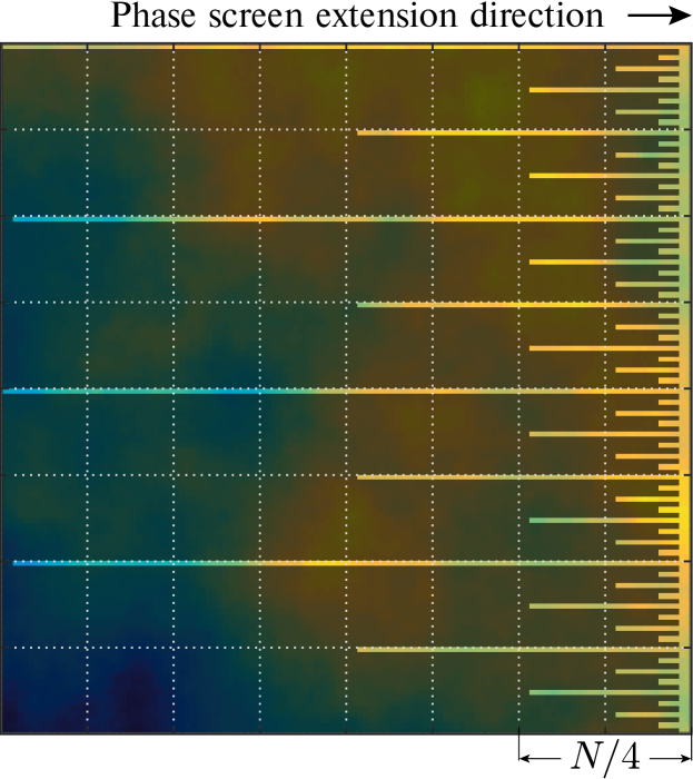
Figure 18: Light areas are pixels taken from the phase screen as the input vector (i.e. the $\mathrm{Z}$ vector in Assémat et al. (2006)).

We slightly modified the method by changing the selection of pixels of the initial phase screen to cover large scales, while not greatly increasing the amount of used RAM. The following selection algorithm was chosen: the two columns of the phase screen closest to the new column being added are taken unchanged, in each of the next four columns only half of the pixels (every second) are selected, in the next eight columns every fourth is selected, and so on. An illustration of this algorithm is shown in Fig. 18. With this selection method, it turned out to be sufficient to take into account only the first $N/4$ columns. Even with this number, the structure function and the variances of the Zernike polynomials of the resulting phase screens agree quite well with the theory. Moreover, the screens generated by this method showed better theory fit than the FFT method (see Fig. 19).

$\ \ \ \ \ \ \ \ \ \ \>L_{0}=2.5$ m

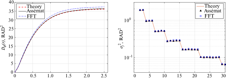
$\ \ \ \ \ \ \ \ \ \ \ L_{0}=10$ m

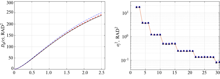
$\ \ \ \ \ \ \ \ \ \ \>L_{0}=25$ m

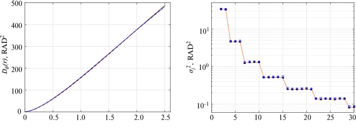
$\ \ \ \ \ \ \ \ \ \ \ L_{0}=100$ m

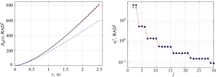
Figure 19: Comparison of structure functions and mode variances of Zernike polynomials with the expected theoretical values (see Winker (1991); Takato & Yamaguchi (1995); Assémat et al. (2006)). Calculated from a sample of 10  000 phase screens generated with Assémat and FFT methods. Cases for $L_{0}$ equal to 2.5, 10, 25 and 100 m are considered. Screen size is 2.5 m (256$\times$256 points).

In this model, in order to approximate the reality better, we generate two phase screens and move the cut sections along them (or extend them) in perpendicular directions. The phase for these two cutouts is then summed. This is done to obtain a realistic characteristic time of phase variations: $r_{0}/V$, where $V$ is the wind speed. Otherwise, when only one phase screen is used, the characteristic time of variations will be $D/V$, where $D$ is the diameter of the telescope aperture.

The speed of movement of the cut out area does not always correspond to the whole number of pixels of the phase screen. In this case, there are two options: one can linearly interpolate the image and shift along it by the required amount, or one can use the Fourier transform, which allows one to shift the image by a fractional number of pixels, since it is known that the Fourier images of the original and shifted images are interconnected by a linear multiplier in frequency space.

4.1.3 Anisoplanatism

Light coming from different points in the sky will pass through different parts of the phase screen, thus resulting in different distortion of the image, which is called anisoplanatism.

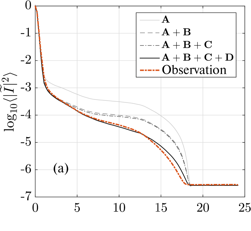
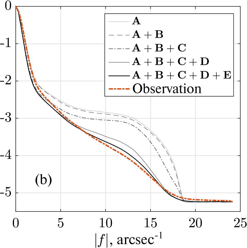
Figure 20: The logarithms of slices of azimuth-averaged normalized model power spectra with successive inclusion of various factors taken into account are compared with real ones (from observations). The horizontal axis shows the modulus of the spatial frequency. Considered factors in the model: A—the CIC noise, photon noise, readout noise, defocus, atmospheric seeing $\beta$, motion of turbulent layers, filter wavelength, B—the finiteness of the exposure value, C— the telescope aberrations, D—the telescope jitter, E—the finiteness of the filter bandwidth. Information about series and simulation parameters: (a)—the H${\alpha}$ filter, stellar magnitude $m_{\rm H\alpha}=-1\,.\!\!^{\rm m}1$, seeing $\beta=1\,.\!\!^{\prime\prime}5$, wind speed $v_{\rm wind}=10$ m s^-1, the value of the telescope jitter $j_{\rm tel}=0\,.\!\!^{\prime\prime}08$, the value of the defocus in the displacements of the secondary mirror $\varepsilon_{M2}=11$ microns, (b)—the $R$ filter, $m_{R}=6\,.\!\!^{\rm m}5$, $\beta=0\,.\!\!^{\prime\prime}62$, $v_{\rm wind}=6$ m s^-1, $j_{\rm tel}=0\,.\!\!^{\prime\prime}085$, $\varepsilon_{M2}=-10$ microns, (c)—the $I$ filter, $m_{I}=10\,.\!\!^{\rm m}2$, $\beta=1^{\prime\prime}$, $v_{\rm wind}=8$ m s^-1, $j_{\rm tel}=0\,.\!\!^{\prime\prime}08$, $\varepsilon_{M2}=11$ microns.

To take into account anisoplanatism, we assume that one of the phase screens is located at an altitude of 10 km, and the second—at zero altitude. Then, for example, if two stars are at an angular distance of $5^{\prime\prime}$ from each other, then at an altitude of 10 km, apertures for each star will be cut out from the first phase screen at a distance approximately equal to 24 cm from each other . On the other hand, the same aperture for both stars will be cut from the second screen.

Based on the object function $O(\alpha_{x},\alpha_{y})$ specified as an array, we calculate the relative position of the centers of the apertures cut out from the phase screen. Then we get the PSF for each star. Every star in object function is then isolated (so that the other sources in object function except the chosen one are ‘‘turned off’’) and convolved with its PSF to get a set of images for each star in the field. Each of these images is an atmospherically distorted image of a star if there were no other stars. Further, we add up all images from this set and obtain final image, taking into account anisoplanatism.

4.1.4 The telescope jitter

With the help of special experiments, described in Appendix B, it was found that the image of a star is ‘‘blurred’’ by about $j_{\rm tel}\approx 0\,.\!\!^{\prime\prime}08$ due to the jitter of the telescope mount. This affects the power spectra in the form of a decrease in the high-frequency region (see Fig. 20). Analysis shows that the telescope oscillations are dominated by harmonics at frequencies of 20, 40, 60 Hz. Naturally, harmonics above 30 Hz will significantly suppress the power spectrum at high spatial frequencies, since typical exposures are 23 ms.

The telescope jitter is taken into account by convolving the image with a segment whose brightness distribution is determined by the ratio of the exposure length and typical amplitude of the jitter.

4.1.5 Other factors

The model takes into account the aberrations of the telescope measured by the Shack–Hartmann sensor (Potanin et al., 2017), and it is also possible to set the defocus value. In addition to atmospheric and optical distortions, we also take into account photon noise, readout noise, and CIC noise (Clock-induced charge, exponentially distributed). We assume that the photon noise follows a Poisson distribution, and the readout noise follows a Gaussian distribution. All the necessary information for their determination (readout noise variance, electron multiplication gain, exposure, detector sensitivity) is taken from real data cubes (FITS observation files).

4.2 Comparison with real data

To validate the model, we compare the power spectra obtained in real observations with the power spectra generated in the model. We sequentially include into consideration various ‘‘refinements’’ of the model, such as the finite filter width, the finite exposure value, and so on. Three observations were selected for comparison in different filters and with different magnitudes of objects.

It can be seen from the graphs (see Fig. 20) that with all the factors taken into account, our model predicts the shape of the power spectra quite accurately. Therefore, we can proceed directly to the study and theoretical comparison of the speckle interferometric capabilities of detectors.

4.3 Comparison of EMCCD and qCMOS

In this Section, we use the model just described to estimate the expected performance of the upgraded instrument compared to the previous version. As a metric, we will consider the ratio $S/N$ in the power spectrum.

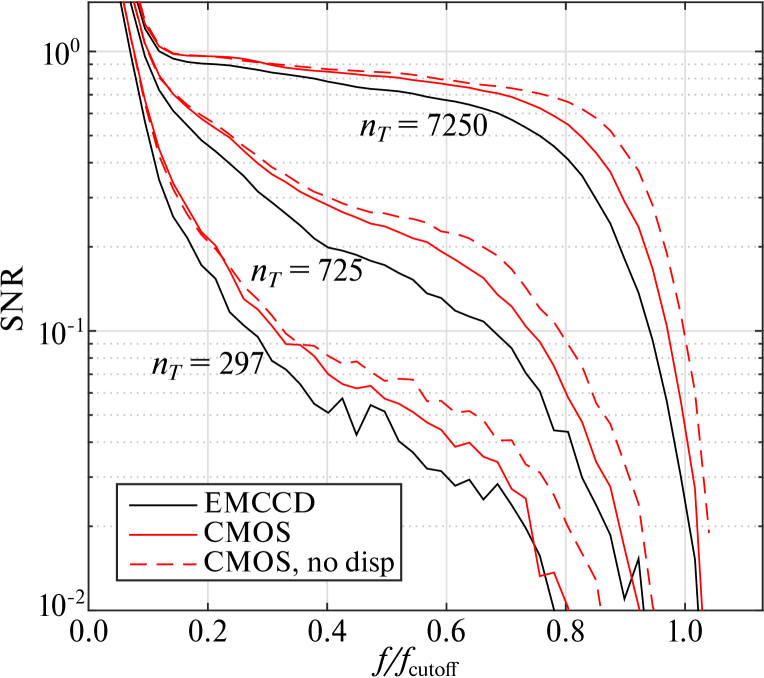
Figure 21: Comparison of the $S/N$ ratio in power spectra per frame for EMCCD, CMOS and CMOS without Wollaston prism dispersion. The horizontal axis shows the modulus of the spatial frequency, normalized to the cutoff frequency $D/\lambda$. The groups of curves correspond to the different average number of photons in the frame $n_{T}$ (indicated in the figure).

The simulation was performed for EMCCD and CMOS, the parameters of which are shown in Table 1. The spectra were calculated over 2000 frames in the region of $140\times 140$ px, which corresponds to $2\,.\!\!^{\prime\prime}8\times 2\,.\!\!^{\prime\prime}8$. The angular scale for ease of comparison was chosen to be the same (as can be seen from Table 1, it differs only slightly). Again, for ease of comparison, we assumed the same number of registered photons per frame, and in both cases the dispersion of the Wollaston prism was taken into account.

The seeing was chosen to be $0\,.\!\!^{\prime\prime}73$, atmospheric model: two layers of equal intensity moving in perpendicular directions at a speed of 10 m s^-1. Exposure—30 ms (the temporal evolution of the image was taken into account), the band $I_{c}$ (the dependence of the image on the wavelength was taken into account).

Figure 21 shows the $S/N$ ratio (SNR) in the power spectrum for objects of three different brightnesses. CMOS provides SNR better than EMCCD by about 1.2–1.6 times. This effect is especially noticeable in the case of faint objects, since the EMCCD efficiency for them is limited by the CIC noise. Figures 11 and 21 confirm the results of the theoretical evaluations carried out in Section 2.5. For bright objects, the difference between CMOS and EMCCD is less pronounced, since atmospheric effect dominates the noise.

5 RESULTS

The classic problem solved by speckle interferometry is to test stars for binarity and, if the latter is detected, to determine the parameters of binarity: separation, position angle, and contrast. The study of binarity is also relevant for UX Ori type variables. The UX Ori type stars are a subclass of young variable stars with sharp chaotic brightness variations, the amplitude of which reaches $3^{\rm m}$. Flux variations in stars of this type are due to the variable absorption of direct stellar radiation in the circumstellar envelope (Grinin et al., 1995). Absorption can occur either in the protoplanetary disk or in dust clouds above the disk—in the dusty disk wind or in the remnants of the protostellar cloud falling onto the disk.

The presence of a stellar component has a significant effect on the protoplanetary disk around a young star. The outer parts of the disk are swept out of the system, the lifetime of the disk is reduced (Kraus et al., 2012; Zagaria et al., 2022). The statistics of exoplanets in binary star systems indirectly indicate the disk-component interaction. Thus, it was found that in stars with a hot Jupiter, the probability of detecting a stellar component with a separation from 50 to 2000 AU is significantly larger than for field stars (Ngo et al., 2016).

Thus, information on binarity in young stars is of great value both for statistical studies and for the astrophysical interpretation of individual objects. From an observational point of view, information about the stellar component must be taken into account when interpreting observations of the UX Ori stars, since the component can distort the flux and polarization measurements. For example, in the very deep eclipses of 2014-2015, the secondary component dominated in the total flux of RW Aur (Dodin et al., 2019).

The Gaia DR3 survey (Gaia Collaboration et al., 2022) has more than 50% completeness only for systems with a separation greater than $0\,.\!\!^{\prime\prime}54$ (Fabricius et al., 2021). At the same time, the diffraction limited resolution of ground-based telescopes in the optical range, which is achievable, in particular, using the speckle interferometry method, is much better. In case of 2.5-m telescope, the diffraction limited resolution is $0\,.\!\!^{\prime\prime}05$–$0\,.\!\!^{\prime\prime}08$. Thus speckle interferometric data are a valuable addition to the Gaia survey.

In the period from 2018 to 2022, speckle interferometric observations of 25 UX Ori stars from the list in Poxon (2015) were carried out with the speckle polarimeter at the 2.5-m telescope. Poxon (2015), in turn, adopted this list from the Internet resource of the American Association of Variable Star Observers AAVSO (Watson et al., 2014). Among the selected stars, only one is present in the Gaia DR3 Part 3 Non-single stars survey (Gaia Collaboration et al., 2022)—the BO Cep star assigned to the Single Lined Spectroscopic binary model with a period of 10.7 days, which gives a separation that lies deep below the diffraction limited resolution of the telescope and undetectable by speckle interferometry.

5.1 Single UX Ori stars—achievable contrast

As a result of observations, binarity was not found in 23 stars from the list. Table 2 shows the results of processing these observations—achievable contrast at a distance of $0\,.\!\!^{\prime\prime}2$ and $1^{\prime\prime}$.

Table 2: UX Ori variables for which binarity has not been found. $\beta$—seeing, $n_{p}$—the number of registered photoelectrons per second; $\epsilon_{\rm lim_{0.2}}$ and $\epsilon_{\rm lim_{1.0}}$—estimates of extreme contrast at a distance of $0\,.\!\!^{\prime\prime}2$ and $1^{\prime\prime}$ respectively.

Object	Time, UT	Filter	$\beta$, arcsec	$n_{p}$	$\epsilon_{\rm lim_{0.2}}$	$\epsilon_{\rm lim_{1.0}}$
ASAS J055007+0305.6	2018/12/02 22:23:37	$I_{c}$	1.24	8.69e+04	3.63	4.79
	2018/12/07 00:14:03	$I_{c}$	1.56	8.21e+04	3.18	5.07
	2019/01/25 21:02:47	$V$	1.50	6.54e+04	2.16	3.86
BF Ori	2018/12/02 23:00:30	$I_{c}$	1.51	2.43e+05	3.82	5.32
	2018/12/02 23:09:27	$I_{c}$	1.38	1.55e+05	3.55	5.50
	2018/12/07 00:23:15	$I_{c}$	1.89	1.18e+05	3.15	4.40
BH Cep	2018/12/02 18:50:59	$I_{c}$	1.12	1.30e+05	2.96	5.07
BO Cep	2018/12/02 18:56:27	$I_{c}$	1.13	5.81e+06	4.61	7.45
CQ Tau	2019/10/27 22:13:18	$I_{c}$	0.83	9.66e+05	4.73	7.46
GM Cep	2018/12/02 19:09:51	$I_{c}$	1.04	3.48e+04	2.44	4.39
	2019/01/20 16:51:46	$I_{c}$	1.27	3.84e+04	3.38	4.49
GSC 05107-00266	2018/07/31 20:39:51	$I_{c}$	1.56	1.36e+05	3.58	5.23
GT Ori	2018/12/02 23:27:43	$I_{c}$	1.24	8.27e+04	2.86	4.75
HQ Tau	2018/12/02 20:24:51	$I_{c}$	1.13	1.76e+05	3.13	5.13
IL Cep	2018/12/02 19:26:34	$I_{c}$	1.10	9.23e+05	4.22	7.20
LO Cep	2018/12/02 19:38:49	$I_{c}$	1.15	2.79e+04	0.34	3.44
PX Vul	2017/03/09 01:49:04	$I_{c}$	0.89	2.69e+05	3.11	6.00
	2018/08/29 20:39:41	$I_{c}$	1.23	1.25e+05	2.36	4.76
	2018/08/29 20:42:55	$V$	1.28	5.66e+04	2.02	3.64
	2020/04/26 01:42:22	$I_{c}$	1.06	1.94e+05	3.31	4.89
	2020/06/10 00:15:59	$I_{c}$	0.71	1.86e+05	3.17	7.03
RR Tau	2018/04/01 17:53:05	880	1.13	1.73e+04	1.95	3.62
	2018/04/01 17:46:49	$I_{c}$	1.04	7.63e+04	3.63	5.38
RZ Psc	2018/12/02 19:56:27	$I_{c}$	1.05	1.03e+05	2.88	5.37
	2019/01/20 17:00:29	880	1.18	1.83e+04	2.19	4.11
SV Cep	2018/12/02 18:40:33	$I_{c}$	1.04	1.48e+05	3.85	6.10
T Ori	2018/12/02 22:53:45	$I_{c}$	1.34	2.22e+05	3.26	4.99
V1012 Ori	2018/12/02 21:51:04	$I_{c}$	1.37	4.23e+04	2.65	4.60
V1977 Cyg	2018/12/02 18:05:48	$I_{c}$	1.24	2.14e+05	3.04	5.48
V517 Cyg	2018/12/02 18:26:04	$V$	1.22	8.28e+03	0.19	2.83
VV Ser	2018/07/31 20:31:22	$I_{c}$	1.41	1.12e+05	3.63	4.71
VX Cas	2018/12/02 20:02:56	$I_{c}$	1.05	8.03e+04	2.94	5.11
WW Vul	2018/08/29 20:31:37	$I_{c}$	1.17	1.64e+05	3.21	5.33
	2018/08/29 20:34:52	$V$	1.47	1.29e+05	2.31	4.04
XX Sct	2018/07/31 20:22:21	$I_{c}$	1.46	5.11e+04	1.47	3.87

5.2 BM And

BM And is a young T Tau-type star and a UX Ori-type variable whose magnitude varies from $m_{V}=11.5$ to $m_{V}=14.0$ (Grinin et al., 1995).

The star was found to have binarity with parameters $\rho\approx 273$ mas, $\mathrm{PA}\approx 249^{\circ}$ (see Figs 22 and 23). For BM And, a total of about 100 observations were made in the $I_{c},R_{c},V$ filters in the period from 2017 to 2022. In the $I_{c}$ filter: 40 magnitude measurements, 42 measurements of binary parameters, $R_{c}$: 38 magnitude measurements, 39 measurements of binary parameters, $V$: 18 magnitude measurements, 23 measurements of binary parameters. The position angle of the star shows a systematic change at a rate of $0\,.\!\!^{\circ}50\pm{0\,.\!\!^{\circ}05}$ per year, no trend was detected in the separation (see Fig.  23). The restoration of the orbit according to our observations is not possible due to the short interval on which they were performed.

According to Gaia DR3 catalogue (Gaia Collaboration et al., 2022) excess astrometry error—5.8 mas—is greater than the parallax value $1.3\pm 0.6$ mas. This is probably due to the simultaneous influence of the binarity and variability of the object. In addition, the scattering envelope, the presence of which is indicated by the variable polarization of the object (Grinin et al., 1995), can also cause a shift in the object’s photocenter (Dodin et al., 2019). Thus, estimating the distance and hence the magnitude of the separation projection onto the celestial sphere in units of length is difficult.

In addition to measuring the contrast between the components, the total magnitude of the system was also estimated by photometry using the standards observed before and after each observation of the object. This made it possible to estimate the magnitudes of both stars in the system (see Fig. 22).

The amplitude of the change in the brightness of the second component obtained from observations turned out to be much smaller than that for the main star of the system. So, in the $I_{c}$ filter, the ratio of the weighted standard deviations of the stellar magnitudes of the components turned out to be 2.1, in the $R_{c}$ filter—1.43, in the $V$ filter—1.4.

The following mean magnitudes of the second component in the $I,R,V$ filters are obtained:

• $m_{2}^{I}=12.67\pm 0.23$, $m_{2}^{R}=13.90\pm 0.44$,

• $m_{2}^{V}=14.96\pm 0.38$.

5.3 NSV 16694

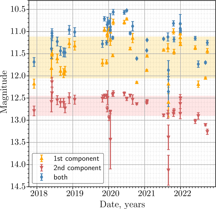
Figure 22: Light curve of BM And and its components in the $I$ filter. The center of the translucent band corresponds to the weighted average of the magnitude of the component in this filter. The half-width of the band is equal to the weighted standard deviation.

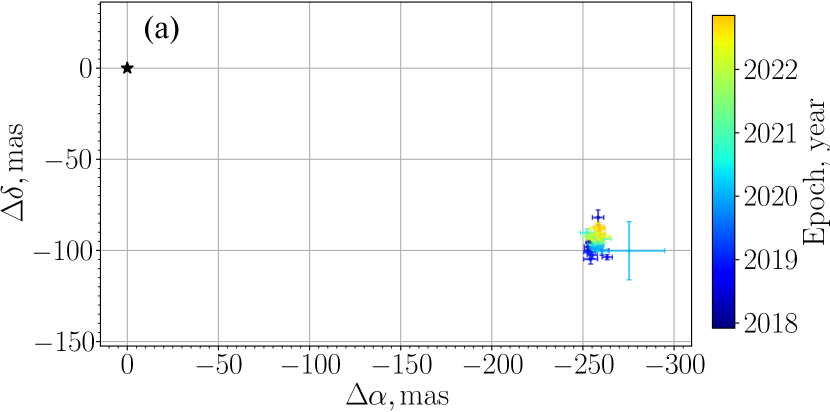
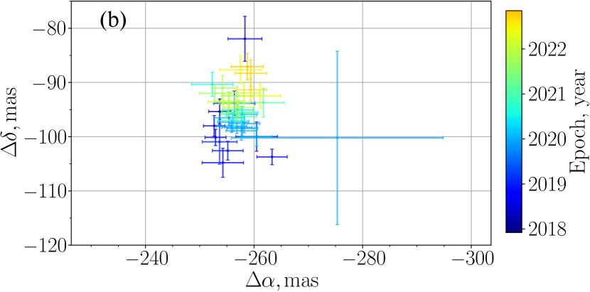
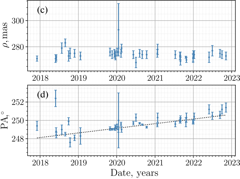
Figure 23: Relative positions of the BM And components over all observations in the $I$ filter. A trend is observed in the position angle, which may be due to the orbital motion of the component. The linear weighted least squares method (LSM) gives the position angle change rate $0\,.\!\!^{\circ}50\pm{0\,.\!\!^{\circ}05}$ per year.

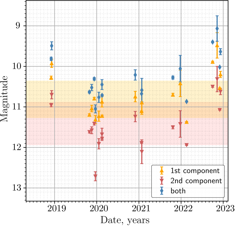
Figure 24: Light curve of NSV 16694 and its components in the $I$ filter. The center of the translucent band corresponds to the weighted average of the magnitude of the component in this filter. The half-width of the band is equal to the weighted standard deviation.

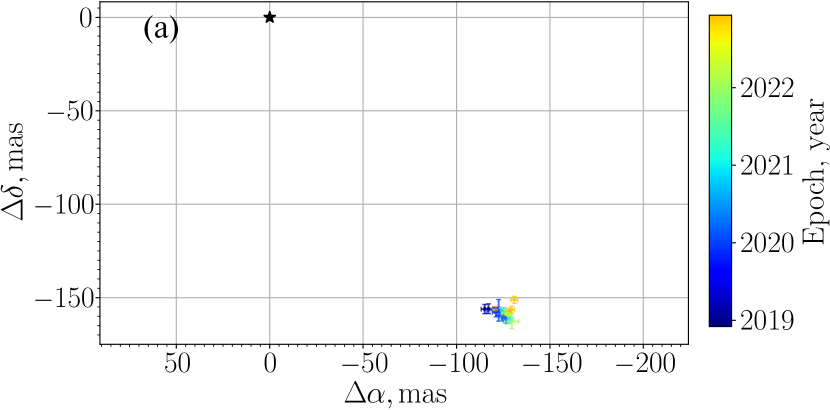
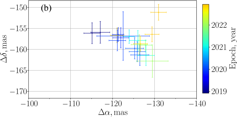
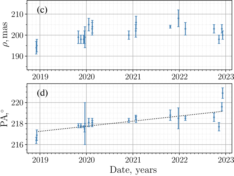
Figure 25: Relative positions of the NSV 16694 components over all observations in the $I$ filter. There is a trend in position angle. A weighted linear least squares method gives the rate of change of the position angle $0\,.\!\!^{\circ}48\pm{0\,.\!\!^{\circ}07}$ per year.

NSV 16694 (TYC 120-876-1, IRAS 05482+0306) is a young stellar object with coordinates (J2000)${\rm RA}=05^{\rm h}50^{\rm m}53\,.\!\!^{\rm s}714$, ${\rm Dec}=+03^{\circ}07^{\prime}29\,.\!\!^{\prime\prime}346$ (Gaia Collaboration et al., 2022) located in the direction of the molecular cloud complex in Orion. In 30–60^′′ to the north of the object lies a nebula, probably associated with the object. In the optical range, the object shows irregular variability (Pojmanski, 2002). The Gaia DR3 catalogue (Gaia Collaboration et al., 2022) for NSV 16694 lacks parallax and proper motion estimates, and the excess astrometry noise is 51 mas.

For NSV 16694, we found binarity with parameters $\rho\approx 202$ mas, ${PA}\approx 218\,.\!\!^{\circ}2$ (see Figs. 24 and 25). From 2019 to 2022, observations were made in the $I$ filter: 19 magnitude measurements, 20 measurements of the binarity parameters, in the $R$ filter: 11 magnitude measurements, 12 measurements of the binarity parameters, in the $V$ filter: 7 magnitude measurements, 8 measurements of the binarity parameters.

In the period from 2019 to 2022, the position angle changed systematically at a rate of $0\,.\!\!^{\circ}48\pm{0\,.\!\!^{\circ}07}$ per year. The magnitudes of the components were estimated independently, similarly to how it was done for BM And. It is noteworthy that in 2019 and the end of 2022, both components of the system were significantly brighter than in 2021 and most of 2022. Coincidence cannot be ruled out to explain such synchronization, especially given the small time frame on which our observations were made. However, a more natural explanation is the hypothesis that either one or both of the components are compact reflection nebulae, the brightness of which is proportional to the brightness of some variable source screened by a dust cloud. This hypothesis is supported by the fact that Magnier et al. (1999) concluded that NSV 16694 is a group of young stellar objects embedded in a protostellar cloud with complex morphology.

6 CONCLUSIONS

In this paper, we investigate the applicability of the Hamamatsu ORCA-quest low-noise CMOS detector in speckle interferometry. The work was carried out in the context of the upgrade of the ‘‘speckle polarimeter’’ instrument mounted on the 2.5-m telescope. We present a detailed description of the instrument, as well as the speckle interferometry technique we use to characterize binary sources. We have carried out a study of the main characteristics of the detector—readout noise, dark current, registration rate. These characteristics have been shown to be within the limits declared by the manufacturer. The readout noise distribution is normal up to three standard deviations.

Previously, the Andor iXon 897 EMCCD detector was used in the speckle polarimeter, so the CMOS Hamamatsu ORCA-quest was considered in comparison with this detector. In speckle interferometry, the main observed quantity is the image power spectrum averaged over a certain series of frames. The ratio $S/N$ in the average power spectrum was chosen as the main metric for comparing detectors. A simple analytical model shows that for bright objects there is practically no difference between CMOS and EMCCD, since in this case the dominant contribution to the noise comes from atmospheric noise, also called speckle noise. Atmospheric noise does not depend on the properties of the detector. For faint objects, CMOS provides a 1.5–2 times better $S/N$ ratio than EMCCD due to the absence of CIC noise (spurious charge) in CMOS.

We also carried out a detailed quantitative analysis of the gain from the use of a CMOS detector using numerical simulation of data acquisition by the Monte Carlo method. The numerical model takes into account all the main effects that affect the operation in the speckle interferometry mode: light propagation through turbulent atmosphere and telescope, readout noise, CIC noise, photon noise, amplification noise. The model was verified by us using the data obtained with a speckle polarimeter. In the process of verification, telescope vibrations were detected, leading to image jitter with an amplitude of up to $0\,.\!\!^{\prime\prime}08$ and a characteristic frequency of 40–60 Hz. Vibrations significantly reduce the $S/N$ ratio in the power spectrum in speckle interferometric observations.

Many CMOS detectors, in particular, the detector considered in this study, operate in a rolling shutter mode, that is, rows are read in turn. Using numerical simulations, we show that the use of a rolling shutter does not significantly affect speckle interferometry measurements.

Some features of the Hamamatsu ORCA–quest that we have found deserve special mention. Thus, the detector shows a significant non-linearity, reaching 15–20% in the region of low fluxes. The correction procedure makes it possible to reduce the non-linearity to 1–2% at signal levels greater than $1~{}e^{-}$. The readout noise in different pixels is not statistically independent, which causes an artifact in the average power spectrum that needs to be corrected.

As an example of an astrophysical problem, we present a survey of 25 young variable stars with the purpose of characterizing their binarity. Of these, 23 objects turned out to be single; the limits of detection of secondary components are given. Binarity was found in BM And and NSV 16694. BM And has a separation of 273 mas, a position angle of $249^{\circ}$, and the binary is probably a gravitationally bound pair. The variability of BM And is due to variations in the brightness of the main component. For NSV 16694, the separation turned out to be 202 mas, the position angle $218\,.\!\!^{\circ}2$. The components of NSV 16694 show synchronous brightness fluctuations, suggesting that at least one of them is a compact reflection nebula.

Among other problems solved using speckle interferometry at the instrument is the refinement of the orbit of the binary asteroid Kalliope-Linus (Emelyanov et al., 2019), refinement of the orbit of the young binary ZZ Tau (Belinski et al., 2022), search for stellar components of exoplanets host stars identified by TESS spacecraft (Cabot et al., 2021; Knudstrup et al., 2022).

APPENDIX A

THE INFLUENCE OF THE ROLLING SHUTTER EFFECT ON THE CONTRAST ESTIMATION

The rolling shutter effect is a consequence of the non-instantaneous sequential reading of detector rows. Even and odd rows are read at the same time, but each pair of such rows takes some time to read, and each next pair of rows is read with a slight delay compared to the previous pair. In the standard and ultra-quiet reading modes, the time spent on a pair of rows is 7.2 microseconds and 172.8 microseconds, respectively.

For example, taking the angular scale equal to $0\,.\!\!^{\prime\prime}02/$px and the separation between two stars equal to $1^{\prime\prime}$, we get that the image of one component will lag behind from the image of the second one by 4.3 ms in the ultra-quiet reading mode if the stars are oriented parallel to the reading direction. This value has the same order of magnitude as the atmospheric coherence time. Therefore, it is necessary to simulate the influence of this effect on the efficiency of speckle interferometric contrast estimation.

To do this, we generated 20 series for three different separations between the components by varying the reading time of a row pair. For each series, standard speckle interferometric processing was applied, from which contrast estimates were obtained. The parameters of the model used to generate the series are as follows:

• Separations between components are $0\,.\!\!^{\prime\prime}35$, $0\,.\!\!^{\prime\prime}7$, $1\,.\!\!^{\prime\prime}05$, the component flux ratio is 0.05. The stars are oriented in the direction of reading.

• Two phase screens at distances of 0 m and 10 000 m, moving in perpendicular directions.

• Wind speed is 10 m s^-1.

• Seeing is $1^{\prime\prime}$.

• No telescope jitter.

• Zero defocus.

• Filter with an infinitely narrow bandwidth.

• The considered wavelength is 822 nm.

• Exposure time is 22 ms.

• The interval between frames increases with the increase in the reading time.

• Telescope aberrations are taken into account.

• Photon noise and readout noise are taken into account. RMSD of the readout noise is 0.27$~{}e^{-}$. Conversion factor is $0.11~{}e^{-}/\mathrm{ADU}$.

• Frame size is $256\times 256$. Angular scale is $0\,.\!\!^{\prime\prime}0205$/px.

• Sampling in time is equal to the time of reading a pair of lines.

• 1000 frames were generated for each series.

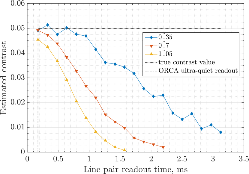
Figure A.1: Estimation of contrast from processing of model series at different reading times of a pair of lines and different separations between components. The vertical dash-dotted line corresponds to the detector’s ultra-quiet reading mode.

It can be seen from Fig. A.1 that the rolling shutter effect clearly influences the speckle contrast estimation. The longer the readout time and the greater the distance between the components, the more the contrast is underestimated (secondary component appears fainter than it is). However, even if we assume a scenario where the separation between the components is $1^{\prime\prime}$ and the ultra-quiet readout mode is used, then the underestimation of the contrast will be only 10%. For larger separations, the contrast can be obtained without using speckle interferometry by approximating the the averaged image.

APPENDIX B

TELESCOPE JITTER

In the course of comparison (see Fig. 20) of real and model power spectra, it turned out that the high-frequency region of the model spectra, other things being equal, is higher than in real observations. We assumed that this excess is due to the fact that the model does not take into account the vibrations of the telescope. We tested this hypothesis in the following way. In good seeing conditions ($\beta<1^{\prime\prime}$) on different dates at different altitudes and azimuths, bright stars were observed with a low exposure and a high frame rate. The value of the electron multiplication was chosen depending on the brightness of the object. Thus, according to our estimates, the frame rate and exposure required to test the hypothesis should be 500 Hz and 0.002 s, respectively.

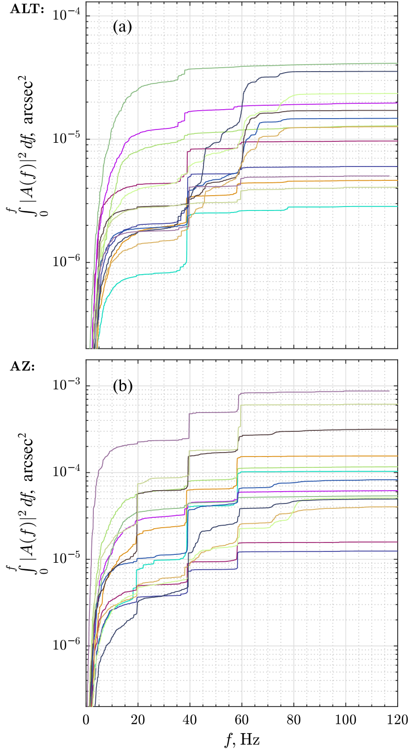
Figure B.1: Cumulative power spectra (that is, the integral of the power spectrum $|A(f)|^{2}$ over frequency) from zero to the frequency of the telescope jitter in altitude and azimuth (in the plane of the sky), units are the arc seconds squared. 14 graphs are superimposed on each other for different series with different conditions and exposures (from 1 ms to 4 ms).

The following processing was applied to the obtained series. Cross-correlation of each ($i\!+\!1$)-th frame with $i$-th was performed. From here we got the offset of each next frame relative to the previous one, that is, the dependence of the offset on time. Next, filtering was performed by moving average with a window size of 0.1 s, that is, by 50 measurements. Then, the filtered ones were subtracted from the original ones in order to eliminate the offsets associated with atmospheric effects.

Spectral analysis of the data obtained (see Fig. B.1) shows that the vibration amplitude in azimuth is indeed greater than in altitude, and reaches $j_{\rm tel}\approx 0\,.\!\!^{\prime\prime}08$. The graph is dominated by harmonics at frequencies of 20, 40, 60 Hz. No significant correlation of these amplitudes with wind speed was found. Moreover, the observations were made on four different days with different weather conditions.

FUNDING

This work was supported by the RSF grant No. 20-72-10011 and the development program of Moscow State University.

CONFLICT OF INTEREST

The authors declare no conflict of interest.

Translated by T. Sokolova

References

- Assémat et al. (2006) Assémat, F., Wilson, R., & Gendron, E. 2006, Optics Express, 14, 988
- Basden & Haniff (2004) Basden, A. G. & Haniff, C. A. 2004, MNRAS, 347, 1187
- Belinski et al. (2022) Belinski, A., Burlak, M., Dodin, A., et al. 2022, MNRAS, 515, 796
- Cabot et al. (2021) Cabot, S. H. C., Bello-Arufe, A., Mendonça, J. M., et al. 2021, AJ, 162, 218
- Dodin et al. (2019) Dodin, A., Grankin, K., Lamzin, S., et al. 2019, MNRAS, 482, 5524
- Efron & Tibshirani (1993) Efron, B. & Tibshirani, R. J. 1993, An Introduction to the Bootstrap, Monographs on Statistics and Applied Probability No. 57 (Boca Raton, Florida, USA: Chapman & Hall/CRC)
- Emelyanov et al. (2019) Emelyanov, N. V., Safonov, B. S., & Kupreeva, C. D. 2019, MNRAS, 489, 3953
- Fabricius et al. (2021) Fabricius, C., Luri, X., Arenou, F., et al. 2021, A&A, 649, A5
- Gaia Collaboration et al. (2022) Gaia Collaboration, Vallenari, A., Brown, A. G. A., et al. 2022, arXiv e-prints, arXiv:2208.00211
- Genet et al. (2016) Genet, R., Rowe, D., Ashcraft, C., et al. 2016, Journal of Double Star Observations, 12, 270
- Grinin et al. (1995) Grinin, V. P., Kolotilov, E. A., & Rostopchina, A. 1995, A&AS, 112, 457
- Harpsøe et al. (2012) Harpsøe, K. B. W., Andersen, M. I., & Kjægaard, P. 2012, A&A, 537, A50
- Hormuth et al. (2008) Hormuth, F., Brandner, W., Hippler, S., & Henning, T. 2008, Journal of Physics Conference Series, 131, 012051
- Howell (2000) Howell, S. B. 2000, Handbook of CCD Astronomy, ed. Howell, S. B.
- Johansson & Gavel (1994) Johansson, E. M. & Gavel, D. T. 1994, in Society of Photo-Optical Instrumentation Engineers (SPIE) Conference Series, Vol. 2200, Amplitude and Intensity Spatial Interferometry II, ed. J. B. Breckinridge, 372–383
- Knudstrup et al. (2022) Knudstrup, E., Serrano, L. M., Gandolfi, D., et al. 2022, A&A, 667, A22
- Kraus et al. (2012) Kraus, A. L., Ireland, M. J., Hillenbrand, L. A., & Martinache, F. 2012, ApJ, 745, 19
- Labeyrie (1970) Labeyrie, A. 1970, A&A, 6, 85
- Law et al. (2006) Law, N. M., Mackay, C. D., & Baldwin, J. E. 2006, A&A, 446, 739
- Magnier et al. (1999) Magnier, E. A., Volp, A. W., Laan, K., van den Ancker, M. E., & Waters, L. B. F. M. 1999, A&A, 352, 228
- Maksimov et al. (2009) Maksimov, A. F., Balega, Y. Y., Dyachenko, V. V., et al. 2009, Astrophysical Bulletin, 64, 296
- Miller (1977) Miller, M. G. 1977, Journal of the Optical Society of America (1917-1983), 67, 1176
- Ngo et al. (2016) Ngo, H., Knutson, H. A., Hinkley, S., et al. 2016, ApJ, 827, 8
- Oscoz et al. (2008) Oscoz, A., Rebolo, R., López, R., et al. 2008, in Society of Photo-Optical Instrumentation Engineers (SPIE) Conference Series, Vol. 7014, Ground-based and Airborne Instrumentation for Astronomy II, ed. I. S. McLean & M. M. Casali, 701447
- Owens (1967) Owens, J. C. 1967, Appl. Opt., 6, 51
- Pojmanski (2002) Pojmanski, G. 2002, Acta Astron., 52, 397
- Potanin et al. (2017) Potanin, S. A., Gorbunov, I. A., Dodin, A. V., et al. 2017, Astronomy Reports, 61, 715
- Poxon (2015) Poxon, M. 2015, The Journal of the American Association of Variable Star Observers, 43, 35
- Safonov et al. (2017) Safonov, B. S., Lysenko, P. A., & Dodin, A. V. 2017, Astronomy Letters, 43, 344
- Scott et al. (2018) Scott, N. J., Howell, S. B., Horch, E. P., & Everett, M. E. 2018, PASP, 130, 054502
- Takato & Yamaguchi (1995) Takato, N. & Yamaguchi, I. 1995, Journal of the Optical Society of America A, 12, 958
- Tokovinin et al. (2010) Tokovinin, A., Cantarutti, R., Tighe, R., et al. 2010, PASP, 122, 1483
- Tokovinin (1988) Tokovinin, A. A. 1988, Zvezdnye interferometry (Stellar interferometers).
- Wasson et al. (2017) Wasson, R., Goldbaum, J., Boyce, P., et al. 2017, Journal of Double Star Observations, 13, 242
- Watson et al. (2014) Watson, C., Henden, A. A., & Price, A. 2014, VizieR Online Data Catalog, B/vsx
- Winker (1991) Winker, D. M. 1991, Journal of the Optical Society of America A, 8, 1568
- Xiang (2014) Xiang, J. 2014, Optical Engineering, 53, 016110
- Zagaria et al. (2022) Zagaria, F., Clarke, C. J., Rosotti, G. P., & Manara, C. F. 2022, MNRAS, 512, 3538