General classification of qubit encodings in ultracold diatomic molecules

Abstract

Owing to their rich internal structure and significant long-range interactions, ultracold molecules have been widely explored as carriers of quantum information. Several different schemes for encoding qubits into molecular states, both bare and field-dressed, have been proposed. At the same time, the rich internal structure of molecules leaves many unexplored possibilities for qubit encodings. We show that all molecular qubit encodings can be classified into four classes by the type of the effective interaction between the qubits. In the case of polar molecules, the four classes are determined by the relative magnitudes of matrix elements of the dipole moment operator in the single molecule basis. We exemplify our classification scheme by considering a new type of encoding of the effective spin-1/2 system into non-adjacent rotational states (e.g., $N=0$ and $N=2$) of polar and non-polar molecules with the same nuclear spin projection. Our classification scheme is designed to inform the optimal choice of molecular qubit encoding for quantum information storage and processing applications, as well as for dynamical generation of many-body entangled states and for quantum annealing.

1 Introduction

Recent experimental progress towards high-fidelity quantum control of ultracold molecules trapped in optical lattices ¹ and tweezers ² has stimulated much interest in using ultracold molecular gases for quantum information science (QIS) applications. The key advantage offered by ultracold molecules lies in their numerous and diverse degrees of freedom, which include not only electronic and hyperfine states (which are also present in atoms), but also vibrational and rotational modes, all of which could be used to encode a qubit. Additionally, these degrees of freedom allow one to encode quantum information into higher-dimensional Hilbert spaces, which could be used either for high-dimensional quantum computing ³ or quantum error correction ⁴. Another crucial advantage of ultracold polar molecules for QIS is afforded by their strong, anisotropic, and tunable electric dipolar (ED) interactions, which can be used to engineer quantum logic gates ^{5, 6, 7} and to generate many-body entangled states ^{8, 9, 10}.

Several types of molecular qubit encodings have been proposed, including into adjacent rotational states ($N=0$ and 1) of the same nuclear/electron spin projection ^{5, 6}, nuclear/electron spin sublevels of a single ($N=0$) rotational state ^{6, 11, 12, 13, 14}, nuclear/electron spin sublevels of adjacent rotational states ($N=0$ and 1) ¹⁰, and vibrational states ^{15, 16}. Robust QI storage is favoured by qubits that are not affected by the long-range ED interaction ^{11, 12}, whereas high-fidelity QI processing (such as robust two-qubit quantum gates) is easier to achieve with strongly interacting qubits ^{6, 7}. The ability to switch between encodings yielding non-interacting and interacting qubits by means of, e.g., microwave pulses ^{17, 18} is a key component of QIS protocols based on ultracold molecules ⁷. This motivates the ongoing search of new qubit encoding schemes. At the same time, the discovery of new qubit encodings may give rise to novel applications of ultracold molecules for quantum computing, such as quantum annealing based on molecules ¹⁹.

Despite the recent proposals ^{6, 12, 13, 14, 10, 15, 16, 7, 19}, there remains a wealth of possibilities for unexplored encodings of qubits into molecular states. For example, qubits can be encoded into non-adjacent rotational levels (e.g., $N=0$ and 2) of the same or different vibronic state, into hyperfine-Zeeman sublevels of the rovibronic states, or even into different rovibrational and hyperfine states in different electronic manifolds. This gives rise to the following question: What are the advantages and limitations of a given molecular qubit encoding for QI storage and processing? This question is relevant because, as mentioned, QI storage and processing impose conflicting requirements on the type of encoding. Specifically, good memory qubits must be well-isolated from an external environment, and their interactions with each other must be minimized to avoid decoherence ²⁰. By contrast, good qubits for processing quantum information must be strongly interacting, with the interactions controllable by external electromagnetic fields ²¹.

Motivated by this question, we propose a classification of molecular qubit encodings based on the ED interaction between the qubits. We show that, given the matrix elements of the dipole moment operator in the single-molecule basis, it is possible to assess the potential utility of any given molecular qubit for QI storage and processing applications. As an example, in Sec. III, we explore a new type of encoding of molecular qubit into non-adjacent rotational states ($N=0$ and 2), which gives rise to several types of encoding according to our classification scheme. In Section IV, we show that similar arguments can be made for higher order long-range couplings by considering electric quadrupole interactions, which are essential for qubit encodings in nonpolar homonuclear molecules. Section V concludes with a brief summary of our main results and discusses several directions for future work.

2 Classification of molecular qubit encodings

We consider an effective spin-1/2 system with the eigenstates $\ket{\downarrow}$ and $\ket{\uparrow}$ comprising a qubit. Choosing a particular encoding amounts to identifying $\ket{\downarrow}$ and $\ket{\uparrow}$ with the physical states of a diatomic molecule, such as electronic, vibrational, rotational, fine, hyperfine, Stark, or Zeeman states. The two-qubit, as well as many-qubit Hamiltonians inherit the properties of the molecular states used for the encoding.

As the strong, anisotropic, and tunable electric dipole-dipole (ED) interaction between molecular qubits is central to their applications in QIS ^{22, 1}, we use the ED interaction as a basis of our classification. The effective ED interaction between two isolated spin-1/2 systems encoded in molecules $i$ and $j$ takes the form of the XXZ Hamiltonian ^{23, 22} (see Appendix A for a derivation)

$$\hat{H}_{ij}=\frac{1-3\cos^{2}\theta_{ij}}{R^{3}}\left[\frac{J_{\perp}}{2}\left(\hat{S}_{i}^{+}\hat{S}_{j}^{-}+\rm{h.c.}\right)+J_{z}\hat{S}_{i}^{z}\hat{S}_{j}^{z}\right.\left.+W\left(\hat{\mathbb{I}}_{i}\hat{S}_{j}^{z}+\hat{S}_{i}^{z}\hat{\mathbb{I}}_{j}\right)+V\hat{\mathbb{I}}_{i}\hat{\mathbb{I}}_{j}\vphantom{\frac{J_{\perp}}{2}}\right],$$ (1)

where $\hat{S}_{i}^{\alpha}$ and $\hat{S}_{j}^{\alpha}$ are the effective spin operators acting in the two-dimensional Hilbert spaces of the $i$-th and $j$-th molecules ($\alpha=\pm,\,z$), $R_{ij}$ is the distance between the molecules and $\theta_{ij}$ is the angle between the quantization vector and the vector connecting the two molecules.

To derive Eq. (1), we assume that the ED interaction between molecules is much weaker than the energy difference between $\ket{\uparrow}$ and $\ket{\downarrow}$. This is a realistic assumption for most molecules trapped in optical lattices and tweezers, for which $|R_{ij}|\geq 500$ nm, and the ED interaction rarely exceeds 1 kHz. As a result, couplings that change the total angular momentum projection of two molecules give rise to energetically off-resonant transitions and can be neglected ²². Examples of such processes include transitions, which transfer angular momentum from molecular rotation to their relative (orbital) motion ($q=\pm 1$ and $q=\pm 2$, see Appendix A). We further assume that the qubit states $\ket{\uparrow}$ and $\ket{\downarrow}$ are isolated, whether by symmetry or by energy detuning, from other molecular states. This is an essential requirement for any QIS protocol.

As shown in previous work (see, e.g., Refs. ^{23, 22}) and detailed in Appendix A for the present discussion, the coupling constants in the effective spin-spin interaction Hamiltonian (1)

$$J_{z} =(d_{\uparrow}-d_{\downarrow})^{2},$$ (2)

$$J_{\perp} =2d_{\uparrow\downarrow}^{2}-|d^{+}_{\uparrow\downarrow}|^{2}-|d^{-}_{\uparrow\downarrow}|^{2},$$ (3)

can be expressed in terms of the matrix elements of the electric dipole moments (EDMs) of the individual molecules with the spherical tensor components $\hat{d}_{p}$ ($\hat{d}_{0}=\hat{d}_{z}$, $\hat{d}_{\pm 1}=\mp(\hat{d}_{x}\pm i\hat{d}_{y})/\sqrt{2}$):

$$\braket{\uparrow}{\hat{d}_{0}}{\uparrow} \equiv d_{\uparrow},\quad\,\,\,\,\,\,\,\,\,\braket{\downarrow}{\hat{d}_{0}}{\downarrow}\equiv d_{\downarrow},$$ (4)

$$\braket{\uparrow}{\hat{d}_{0}}{\downarrow} \equiv d_{\uparrow\downarrow},\quad\braket{\uparrow}{\hat{d}_{\pm 1}}{\downarrow}\equiv d^{\pm}_{\uparrow\downarrow}.$$ (5)

Significantly, the Ising coupling constant $J_{z}$ depends on the difference between the diagonal matrix elements of the EDM in the qubit basis, and the spin exchange coupling $J_{\perp}$ scales with the square of the off-diagonal (or transition) matrix element. In practice, in the absence of mixing between angular momentum projection states, either $d_{\uparrow\downarrow}$ or $d^{\pm}_{\uparrow\downarrow}$ vanish, so either the first or the last two terms on the right-hand side of Eq. (3) are different from zero. The terms parameterized by the constants $W=(d_{\uparrow}^{2}-d_{\downarrow}^{2})/2$ and $V=(d_{\uparrow}+d_{\downarrow})^{2}/4$ in Eq. (1) result in the overall energy shift for a homogeneous ensemble of pinned molecules ²², so we neglect them in the following.

The effective ED interaction in the form of Eq. (1) can be used in combination with Eqs. (2)-(3) to classify the different qubit encodings. To this end, we first note that if $J_{z}=0$ and $J_{\perp}=0$, the ED interaction between the qubits is identically zero. According to Eq. (1) the vanishing of the ED interaction requires the following two conditions to be simultaneously fulfilled: $d_{\uparrow}=d_{\downarrow}$ and $d_{\uparrow\downarrow}=0$. Thus, all qubit encodings, for which the diagonal elements of the EDM are equal and the off-diagonal matrix elements vanish, will have zero ED interaction. Because of this, we expect such qubit encodings to have long coherence times, which can be advantageous for long-term quantum information storage applications (memory qubits).

We use a pair of categorical variables $Z$ and $X$ to characterize the encodings based on Eq. (1). The variable $Z$ takes the value of 0 if the Ising interaction is zero ($J_{z}=0$) and 1 otherwise. Similarly, the variable $X$ takes the value of 0 if the spin-exchange interaction is zero ($J_{\perp}=0$) and 1 otherwise. This gives rise to four possible encodings listed in Table 1. For example, the encoding, for which $J_{z}=J_{\perp}=0$, is classified as 0/0. We can also refer to it as interactionless because, as shown above, the qubit states are not coupled by the long-range ED interaction.

As an example of the 0/0 encoding, consider the nuclear spin sublevels of the ground ($N=0$) rotational state of alkali-dimer molecules. In the high magnetic field limit, the eigenstates of these molecules can be written as $|NM_{N}\rangle|I_{1}M_{I_{1}}\rangle|I_{2}M_{I_{2}}\rangle=|NM_{N},M\rangle$, where $|NM_{N},M\rangle$ are the eigenstates of rotational angular momentum $\hat{N}$ and its $z$-component $\hat{N}_{z}$, $|I_{\alpha}M_{I_{\alpha}}\rangle$ are the eigenstates of the nuclear spin operators $\hat{I}_{\alpha}^{2}$ and $\hat{I}_{\alpha_{z}}$ of the $\alpha$-th nucleus ($\alpha=1,2$), and $M=\{M_{I_{1}},M_{I_{2}}\}$ is a collective nuclear spin quantum number ²⁴. The nuclear spin qubit states are then encoded as $\ket{\uparrow}=\ket{00,M}$ and $\ket{\downarrow}=\ket{00,M^{\prime}}$ with $M\neq M^{\prime}$. With this encoding, $d_{\uparrow}=d_{\downarrow}$ because both the $\ket{\uparrow}$ and $\ket{\downarrow}$ states have $N=0$, and $d_{\uparrow\downarrow}=0$ because the EDM operators $\hat{d}$ and $\hat{d}_{\pm}$ are diagonal in the nuclear spin quantum number (for concreteness, we focus on the $q=0$ spherical tensor component of the EDM operator $\hat{d}=\hat{d}_{0}$, noting that the $q={\pm 1}$ components can be treated in a similar way)

$$\langle NM_{N},M|\hat{d}|N^{\prime}M_{N}^{\prime},M^{\prime}\rangle=\langle NM_{N}|\hat{d}|N^{\prime}M_{N}^{\prime}\rangle\delta_{MM^{\prime}}$$ (6)

and the nuclear spin qubit states have $M\neq M^{\prime}$. Here, $\delta_{MM^{\prime}}=\delta_{M_{I_{1}}M_{I_{1}}^{\prime}}\delta_{M_{I_{2}}M_{I_{2}}^{\prime}}$. In the presence of an external dc electric field $E$, the expectation values $d_{\uparrow}$ and $d_{\downarrow}$ are different from zero, but $d_{\uparrow}=d_{\downarrow}$, so both $J_{z}$ and $J_{\perp}$ vanish even at $E>0$. This effectively cancels the long-range ED interactions, leading to long coherence times of several seconds or longer, as observed experimentally for ultracold trapped KRb ^{17, 25}, RbCs ¹², NaK¹¹, and NaRb ²⁶ molecules.

As noted above, in order for two qubits to interact via the long-range ED interaction (1), either $J_{z}$ or $J_{\perp}$ (or both) must be nonzero. This leads to three other types of encodings listed in Table 1, which we now proceed to analyze.

First, if $J_{z}=0$ and $J_{\perp}\neq 0$, the effective spin-spin interaction between the $i$-th and $j$-th qubits (1) takes the form of the long-range spin-exchange interaction ^{27, 23, 22}

$$H_{ij}=\frac{1-3\cos^{2}\theta_{ij}}{R^{3}}\left[\frac{J_{\perp}}{2}\left(S_{i}^{+}S_{j}^{-}+\rm{h.c.}\right)\right],$$ (7)

Because $J_{\perp}\neq 0$ and $J_{z}=0$, this encoding can be classified as 0/1 (see Table 1). This is by far the most common type of encoding considered in the literature to date. As an example, the encoding into adjacent rotational states $\ket{\uparrow}=\ket{00,M}$ and $\ket{\downarrow}=\ket{1M_{N},M^{\prime}}$ with $M=M^{\prime}$ was originally proposed in a seminal paper by DeMille ⁵. It follows from Eq. (6) that the off-diagonal EDM matrix element does not vanish

$$d_{\uparrow\downarrow}=\langle 00,M|\hat{d}|1M_{N},M\rangle=\langle 00|\hat{d}|1M_{N}\rangle\neq 0,$$ (8)

and hence $J_{\perp}\propto d_{\uparrow\downarrow}^{2}\neq 0$. The diagonal EDM matrix elements in the adjacent rotational state encoding are zero in the absence of an external $E$ field because the two rotational states have a definite parity. As a result, $J_{z}=0$ and the adjacent rotational state encoding can be classified as 0/1. In nonzero electric field, $d_{\uparrow}\neq d_{\downarrow}$ and thus $J_{z}\neq 0$, and the type of encoding changes to 1/1 (see below). This demonstrates that applying an external $E$ field can cause interconversion between the different types of encodings. We will see another example of this “encoding crossover” in Sec. III.

Second, if $J_{z}\neq 0$ and $J_{\perp}=0$, the effective spin-spin interaction between the $i$-th and $j$-th qubits (1) takes the form of the long-range Ising interaction ¹⁰

$$H_{ij}=\frac{1-3\cos^{2}\theta_{ij}}{R^{3}}J_{z}S_{i}^{z}S_{j}^{z},$$ (9)

Because $J_{z}\neq 0$ and $J_{\perp}=0$, this is a 1/0 encoding (see Table 1). Until very recently, this type of encoding has been virtually unexplored, unlike the standard 0/0 and 0/1 encodings ^{12, 5}. One example of such encoding, which we will refer to as spin-rotational, can be realized by the lowest two rotational states with different nuclear spin projections ¹⁰, i.e., $\ket{\uparrow}=\ket{00,M}$ and $\ket{\downarrow}=\ket{1M_{N},M^{\prime}}$ with $M\neq M^{\prime}$ (note that in the standard encoding into adjacent rotational states, $M=M^{\prime}$).

Equation (9) shows that encodings of the 1/0 type, such as the spin-rotational encoding, naturally give rise to the long-range Ising interaction ¹⁰. Dynamical evolution of quantum many-body systems interacting via the Ising Hamiltonian generates cluster-state entanglement ²⁸. Cluster states are universal entangled resource states for measurement-based quantum computation ^{28, 29}. The Ising interaction (9) can also be used to implement universal two-qubit quantum logic gates (Ising gates), which have been explored in the context of nuclear magnetic resonance (NMR)-based quantum computation ³⁰. These interactions can also be used for more complex QI protocols, such as, for example, protocols based on qubits encoded into states of multiple molecules, which can be used for engineering transverse-field Ising models for applications such as quantum annealing ¹⁹.

Finally, when both $J_{\perp}$ and $J_{z}$ are nonzero, the effective spin-spin interaction contains both the Ising and spin-exchange terms, leading to the 1/1 type encoding, in which all the terms in the XXZ Hamiltonian are nonzero. As stated above, one common example of such encoding is furnished by the adjacent rotational states with the same nuclear spin projection ($\ket{\uparrow}=\ket{00,M}$ and $\ket{\downarrow}=\ket{1M_{N},M^{\prime}}$ with $M=M^{\prime}$) in nonzero electric field (in Sec. III, we will consider a less familiar example of encoding into non-adjacent rotational states). In this encoding, $d_{\uparrow\downarrow}\neq 0$ and the presence of the field ensures that $d_{\uparrow}\neq d_{\uparrow}$, and thus $J_{z}\neq 0$. The property of both the Ising and spin-exchange interactions being different from zero is advantageous for a number of applications, such as dynamical generation of many-body spin-squeezed states ^{9, 10}, which can be used to achieve metrological gain over the standard quantum limit ^{31, 32}. At the same time, the coherence properties of 1/1 type qubits (as well as those of the 1/0 and 0/1 types) may be limited by the strong and long-range ED interaction, which is experimentally challenging to turn on and off.

Qubit type	Examples	Advantages	Limitations
0/0 (interactionless)	Nuclear spin sublevels ($N=0$)	Coherence time	Two-qubit gates
$d_{\uparrow}=d_{\downarrow}$, $d_{\uparrow\downarrow}=0$	Non-adjacent rotational states, $E=0$	QI storage
0/1 (spin-exchange)	Adjacent rotational states, $E=0$(1)	Two-qubit gates	Coherence time
$d_{\uparrow}=d_{\downarrow}$, $d_{\uparrow\downarrow}\neq 0$		Entanglement
1/0 (Ising)	Spin-rotational states ($N=0,1$)(2)	Two-qubit gates	Coherence time
$d_{\uparrow}\neq d_{\downarrow}$, $d_{\uparrow\downarrow}=0$	Non-adjacent rotational states(3)	Entanglement
1/1 (XXZ)	Adjacent rotational states, $E>0$(1)	Two-qubit gates	Coherence time
$d_{\uparrow}\neq d_{\downarrow}$, $d_{\uparrow\downarrow}\neq 0$	Non-adjacent rotational states, $E>0$(4)	Entanglement

Table 1: Qubit encoding classification based on the effective ED interqubit coupling.

3 Qubit encoding into non-adjacent rotational levels

To illustrate the application of the proposed classification scheme, we consider a previously unexplored type of qubit encoding into non-adjacent rotational levels of a ${}^{1}\Sigma$ molecule. The Hamiltonian of a ${}^{1}\Sigma$ molecule in the vibrational ground state placed in dc electric field $\bm{E}$ can be written as

$$\hat{H}=B_{e}\hat{N}^{2}-\bm{E}\cdot\bm{d}$$ (10)

where $B_{e}$ is the rotational constant, and $\bm{d}$ is the dipole moment of the molecule. Figure 1 shows the lowest nine eigenvalues of Hamiltonian (10) as functions of the effective electric field $\eta\equiv{dE}/{B_{e}}$. These states correspond to rotational states with $N=0,1$ and $2$ at zero field.

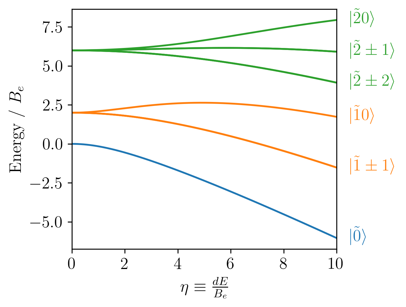
Figure 1: Energy levels of a ${}^{1}\Sigma$ molecule as functions of the effective electric field.

The interaction of molecules with the electric field couples rotational states $\ket{NM_{N}}$ with the same projection ($M_{N}$) to yield dc field-dressed (or pendular) states ^{33, 22}

$$\ket{\tilde{N}M_{N}}=\sum_{N}c_{N}\ket{NM_{N}}.$$ (11)

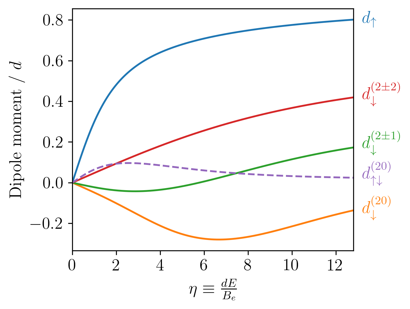
Figure 2: Non-zero EDM matrix elements of $\hat{d}_{0}$ for a ${}^{1}\Sigma$ molecule as a function of the effective electric field.

The choice of $\ket{\downarrow}=\ket{\tilde{0}0}$ leaves five choices for $\ket{\uparrow}$ from the manifold correlating at zero field with $N=2$, including $\ket{\tilde{2}0},\ket{\tilde{2}\pm 1}$ and $\ket{\tilde{2}\pm 2}$. The matrix elements of the dipole operators in the rotational basis states are calculated as

$$\braket{N^{\prime}M_{N^{\prime}}}{\hat{d}_{p}}{NM_{N}}=d(-1)^{M_{N^{\prime}}}\sqrt{(2N^{\prime}+1)(2N+1)}\begin{pmatrix}N^{\prime}&1&N\\ -M_{N^{\prime}}&p&M_{N}\end{pmatrix}\begin{pmatrix}N^{\prime}&1&N\\ 0&0&0\end{pmatrix}$$ (12)

where $d$ is the permanent dipole moment of the molecule. The $3j$-symbols in Eq. (12) vanish if $|N^{\prime}-N|<1$ and $M_{N}+p\neq M_{N^{\prime}}$. The non-zero EDM matrix elements of $\hat{d}_{0}$ as a function of the effective electric field $\eta\equiv{dE}/{B_{e}}$ are displayed for the three possible encodings in Fig. 2, where

$$d_{\uparrow} =\braket{\tilde{0}0}{\hat{d}_{0}}{\tilde{0}0},$$ (13)

$$d_{\downarrow}^{(NM_{N})} =\braket{\tilde{N}M_{N}}{\hat{d}_{0}}{\tilde{N}M_{N}},$$ (14)

$$d_{\uparrow\downarrow}^{(NM_{N})} =\braket{\tilde{0}0}{\hat{d}_{0}}{\tilde{N}M_{N}}.$$ (15)

The transition matrix elements of $\hat{d}_{p}$ ($d_{\uparrow\downarrow}$ and $d_{\uparrow\downarrow}^{\pm}$) vanish for states with $M_{N}\neq p$. Therefore, $d_{\uparrow\downarrow}$ is only non-zero when $\ket{\downarrow}=\ket{\tilde{2}0}$ and $d_{\uparrow\downarrow}^{\pm}$ is only non-zero when $\ket{\downarrow}=\ket{\tilde{2}\pm 1}$. Note that $d_{\uparrow\downarrow}\neq 0$ at $E>0$ because the states $\ket{\tilde{0}0}$ and $\ket{\tilde{2}0}$ couple through the intermediate state $\ket{\tilde{1}0}$. All transition dipole matrix elements vanish for $\ket{\downarrow}=\ket{\tilde{2}\pm 2}$. All diagonal matrix elements are zero for bare rotational states at zero field.

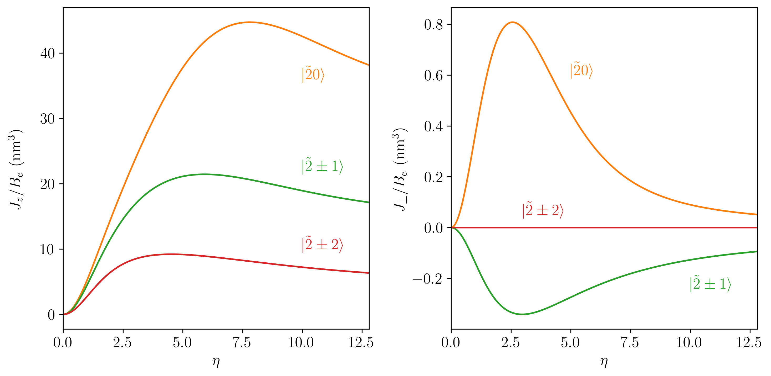
Figure 3: Couplings $J_{z}$ (left) and $J_{\perp}$ (right) as a function of the effective electric field, using the ground rotational state and the indicated rotational states of a polar ${}^{1}\Sigma$ molecule to encode the qubits.

As follows from Fig. 2, qubits spanning the $\tilde{N}=0,\tilde{N}=2$ pairs permit two classes of encoding: the 0/0 encoding at vanishing electric field, 1/0 encoding and 1/1 encoding, depending on the $\ket{\uparrow}$ state. To illustrate this more clearly, we calculate the parameters of the XXZ interaction of Eq. (1) using Eqs. (2)-(3) and the EDM matrix elements. Figure 3 shows the couplings $J_{z}$ and $J_{\perp}$ as functions of the effective electric field. As described in Eq. (2), the Ising coupling between qubits grows as a function of the difference in the diagonal matrix elements of the qubit states. This is observed in the left panel of Fig. 3, as $J_{z}$ is consistently maximized for $\ket{\downarrow}=\ket{\tilde{2}0}$. On the other hand, $J_{\perp}$ corresponds to the square of the off-diagonal EDM matrix elements. As expected, $J_{\perp}$ is equal to zero when $\ket{\downarrow}=\ket{\tilde{2}2}$ regardless of the $E$-field, while $J_{\perp}$ is positive for $\ket{\downarrow}=\ket{\tilde{2}0}$ and negative for $\ket{\downarrow}=\ket{\tilde{2}0}$ at non-zero $E$-field. However, both perpendicular couplings are maximized at intermediate field strengths, and diminish in strong fields.

4 Quadrupole-quadrupole interaction

The classification scheme proposed here can be extended to other long-range interactions than the ED interaction. As an example, we consider in the present section the quadrupole-quadrupole (QQ) interaction. This interaction is the leading long-range interaction between homonuclear molecules, which do simultaneously possess even/odd $N$ state manifolds and which therefore can particularly benefit from the qubit encoding introduced in the preceding section. Previous theoretical work has shown that QQ interactions of nonpolar atoms and molecules in two-dimensional optical lattices can give rise to exotic topological phases ³⁴.

As shown in Appendix B, the QQ interaction leads to the same XXZ model as given by Eq. (1). However, the model parameters must now be expressed in terms of the matrix elements of the quadrupole moment, yielding the following relations:

$$J_{z} =(q_{\uparrow}-q_{\downarrow})^{2},$$ (16)

$$J_{\perp} =2\left[6q_{\uparrow\downarrow}^{2}-4\left[|q_{\uparrow\downarrow}^{+1}|^{2}+|q_{\uparrow\downarrow}^{-1}|^{2}\right]+\left[|q_{\uparrow\downarrow}^{+2}|^{2}+|q_{\uparrow\downarrow}^{-2}|^{2}\right]\right],$$ (17)

Thus, the same classification scheme can be applied to qubits encoded in non-polar molecules interacting through QQ couplings with analogous conditions on the vanishing of $J_{z}$ and $J_{\perp}$, which can be analyzed by considering the matrix elements of the quadrupole moment in the single-molecule basis.

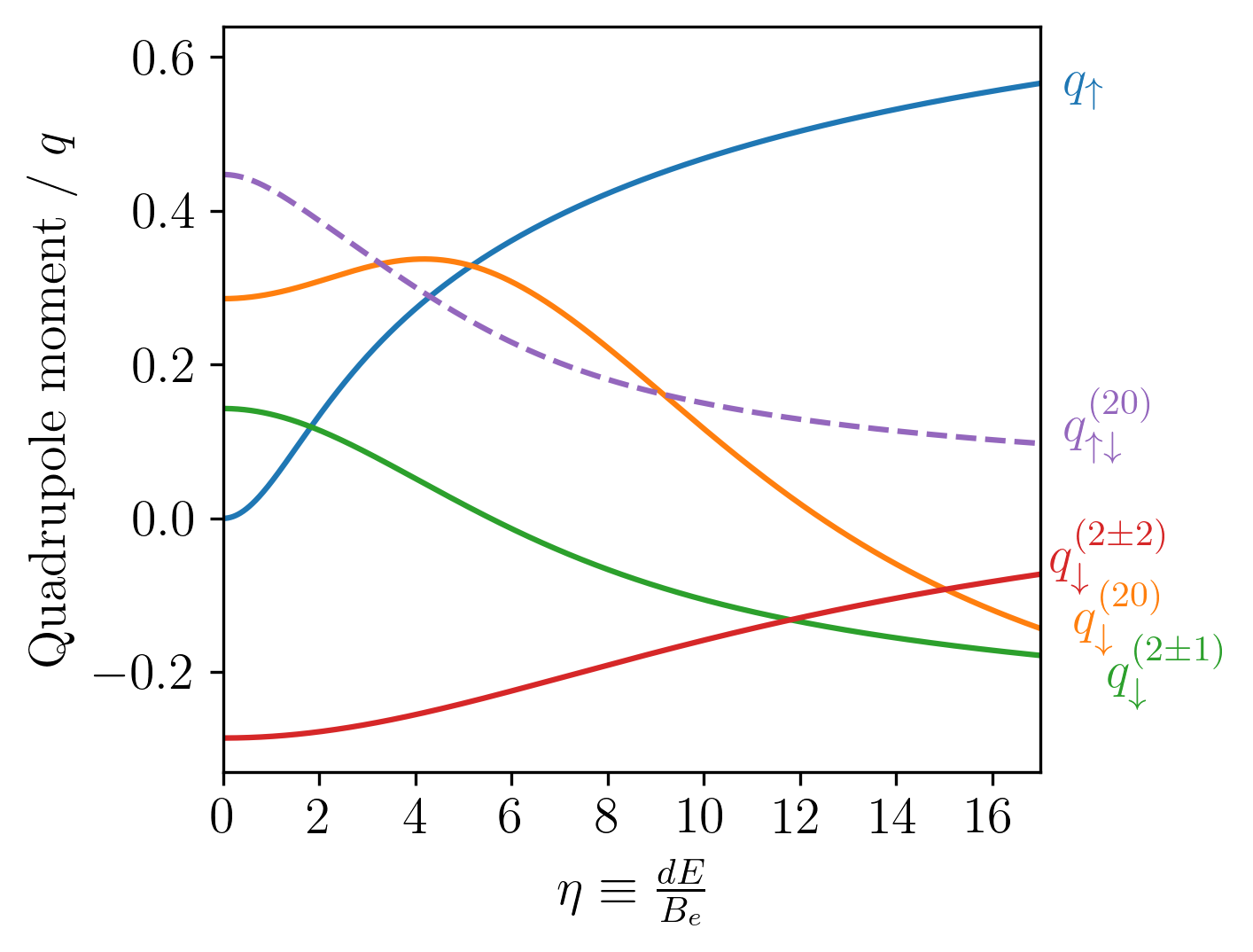
Figure 4: Non-zero quadrupole matrix elements of $\hat{q}_{0}$ as a function of the effective electric field.

The matrix elements of the quadrupole operators in the rotational basis states are calculated as

$$\braket{N^{\prime}M_{N^{\prime}}}{\hat{q}_{p}}{NM_{N}}= q(-1)^{M_{N^{\prime}}}\sqrt{(2N^{\prime}+1)(2N+1)}$$

$$\times\begin{pmatrix}N^{\prime}&2&N\\ -M_{N^{\prime}}&p&M_{N}\end{pmatrix}\begin{pmatrix}N^{\prime}&2&N\\ 0&0&0\end{pmatrix}$$ (18)

where $q$ is the permanent quadrupole moment of the molecule. The $3j$-symbols in Eq. (18) vanish if $|N^{\prime}-N|<2$ and $M_{N}+p\neq M_{N^{\prime}}$. The non-zero EDM matrix elements of $\hat{q}_{0}$ as a function of the effective electric field $\eta\equiv\frac{dE}{B_{e}}$ are displayed for the three possible encodings in Fig. 4, where

$$q_{\uparrow} =\braket{\tilde{0}0}{\hat{q}_{0}}{\tilde{0}0},$$ (19)

$$q_{\downarrow}^{(NM_{N})} =\braket{\tilde{N}M_{N}}{\hat{q}_{0}}{\tilde{N}M_{N}},$$ (20)

$$q_{\uparrow\downarrow}^{(NM_{N})} =\braket{\tilde{0}0}{\hat{q}_{0}}{\tilde{N}M_{N}}.$$ (21)

The transition matrix elements of $\hat{q}_{p}$ ($q_{\uparrow\downarrow}$, $q_{\uparrow\downarrow}^{\pm 1}$ and $q_{\uparrow\downarrow}^{\pm 2}$) vanish for states with $M_{N}\neq p$. Therefore, $q_{\uparrow\downarrow}$ is only non-zero when $\ket{\downarrow}=\ket{\tilde{2}0}$, $q_{\uparrow\downarrow}^{\pm 1}$ is only non-zero when $\ket{\downarrow}=\ket{\tilde{2}\pm 1}$ and $q_{\uparrow\downarrow}^{\pm 2}$ is only non-zero when $\ket{\downarrow}=\ket{\tilde{2}\pm 2}$.

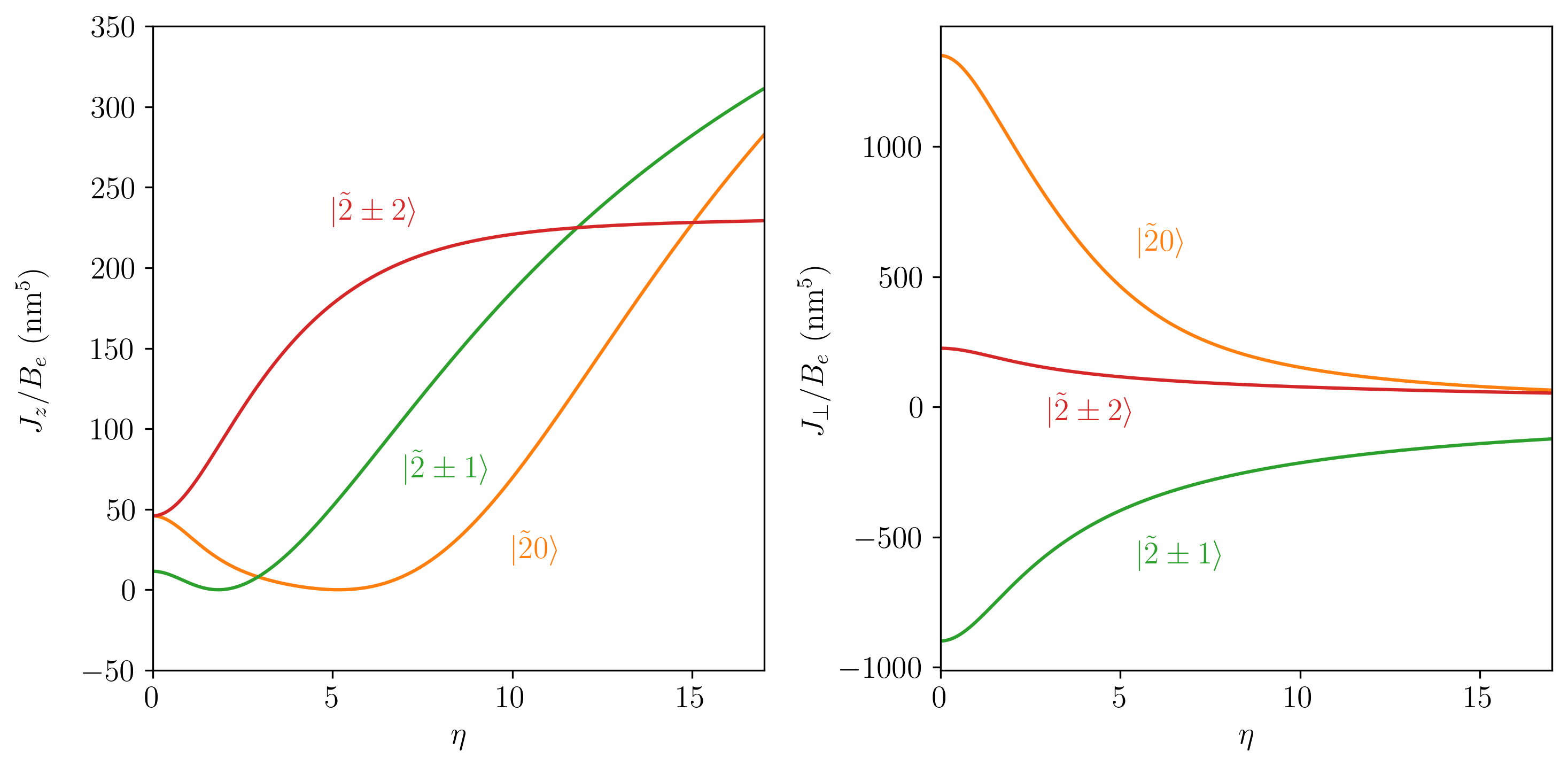
Figure 5: Quadrupole contribution to couplings $J_{z}$ (left) and $J_{\perp}$ (right) as a function of the effective electric field, using the ground rotational state and the indicated rotational states to encode the qubits.

To illustrate the possible types of encoding achievable with homonuclear molecules, we calculate the parameters of the XXZ interaction of Eq. (1) using Eqs. (16-17) and the quadrupole matrix elements. Figure 5 shows the couplings $J_{z}$ and $J_{\perp}$ as functions of the effective electric field. As described in Eq. (16), the Ising coupling between qubits grows as a function of the difference in the diagonal matrix elements of the qubit states. On the other hand, $J_{\perp}$ corresponds to the square of the off-diagonal quadrupole matrix elements. As expected, $J_{\perp}$ is positive for $\ket{\downarrow}=\ket{\tilde{2}0}$ and $\ket{\downarrow}=\ket{\tilde{2}\pm 2}$ and negative for $\ket{\downarrow}=\ket{\tilde{2}\pm 1}$ at non-zero $E$-field. However, all three perpendicular couplings are maximized at low field strengths, and diminish in strong fields. It can be observed that the QQ interaction permits the following types of encoding based on the $\tilde{N}=0$ and $\tilde{N}=2$ states: 0/1, 1/1 and 1/0.

Finally, we note that for typical lattice spacings used in current experiments ($\simeq 500-1000$ nm), the QQ interaction is on the order of $\leq$1 Hz, which is two-three orders of magnitude weaker than the ED interaction between polar molecules. Despite its weakness, the effective QQ interaction Hamiltonian has the same form as the ED Hamiltonian, and can therefore be used (at least in principle) to generate useful many-body entangled states of nonpolar molecules in the same way as the ED interaction of polar molecules ^{9, 10}. In order to ensure robust dynamical evolution toward such entangled states, the evolution timescale should be much shorter than the coherence time of non-adjacent rotational state superpositions ^{8, 10}.

5 Conclusions

Molecules are complex quantum systems that feature multiple energy scales ranging from tens of Hz (hyperfine, Zeeman, and tunneling doublet structure) to thousands of THz (electronic structure). In addition, intermolecular interactions at short range are described by multidimensional potential energy surfaces (PESs), whose accurate description requires sophisticated quantum chemistry techniques and fitting methods. However, the long-range physics of intermolecular interactions of relevance to current QIS experiments in optical lattices and tweezers ^{1, 2} is completely described by the well-established multipole expansion. The lowest leading order in the multipole expansion for neutral (uncharged) polar molecules is represented by the ED interaction, and the next leading orders by the EQ and QQ interactions.

For qubit-based QIS applications, the molecule is reduced to a two-level system (the qubit), whose effective spin-1/2 levels can be encoded into the electronic, vibrational, rotational, fine, hyperfine, Stark, or Zeeman states. Different choices of encoding give rise to different flavors of the ED interaction between the qubits. Here, we have shown that all possible encodings can be classified into 4 types based on the flavor of the effective ED interaction they give rise to.

Our classification is based on two realizations. First, the general interaction between molecular qubits is completely determined by the ED Hamiltonian in the effective two-qubit basis. Second, the form of this Hamiltonian depends only on the matrix elements of the EDM of the individual molecules in a given encoding. The general ED Hamiltonian takes the form of the iconic XXZ Heisenberg model of quantum magnetism ²² with the Ising and spin-exchange coupling parameters $J_{z}$ and $J_{\perp}$ expressed in terms of the diagonal ($d_{\uparrow}$, $d_{\downarrow}$) and off-diagonal ($d_{\uparrow\downarrow}$) EDM matrix elements of each of the individual molecules. As a result, the flavor of the ED interaction is completely determined by single-molecule EDM matrix elements in the qubit basis, regardless of the precise nature of qubit states.

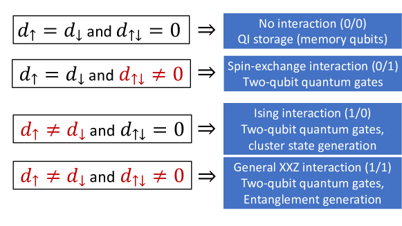
Figure 6: Molecular qubit encoding classification diagram. To classify a qubit, first determine the values of $d_{\uparrow}$, $d_{\downarrow}$, and $d_{\uparrow\downarrow}$, and locate the relevant box in the left column. The qubit encoding type is indicated to the right of each box.

It follows from Eq. (1) that there can be 4 flavors of the ED interaction depending on whether or not the coupling constants $J_{z}$ and $J_{\perp}$ are equal to zero. If $J_{z}=J_{\perp}=0$, no ED interaction is present between the qubits, and we classify them as interactionless (0/0). In the later case, three types of the ED interaction can be distinguished based on whether the values of $|d_{\uparrow}-d_{\downarrow}|$ and $d_{\uparrow\downarrow}$ are zero (see Table 1). We classify these three types as Ising (1/0), spin-exchange (0/1), and XXZ (1/1).

To identify the type of molecular qubit encoding, the reader can use the diagram shown in Fig. 6. One begins by calculating the matrix elements of the EDM in the qubit basis $d_{\uparrow},d_{\downarrow}$, and $d_{\uparrow\downarrow}$ and locating the corresponding box on the left-hand side of the diagram. The right-hand side of the diagram identifies the type of qubit encoding and outlines its possible applications, with a more detailed discussion provided in Sec. 2.

To illustrate our classification scheme, we have considered a new type or molecular qubit encoding into non-adjacent rotational states of a polar diatomic molecule (such as $N=0$ and $N=2$). At zero external electric field, all EDM matrix elements vanish due to the parity selection rules and this encoding can be classified as interactionless (or 0/0 type), which can be useful as a storage (memory) qubit. In the presence of a dc electric field, the qubit is converted into type 1/1 due to both diagonal and off-diagonal EDM matrix elements being nonzero. However, when the projection $M_{N}$ of the rotational angular momentum of the qubit states differs by two or more, the off-diagonal matrix elements of the EDM vanish identically, and the encoding type changes to 1/0.

In future work, it would be interesting to apply our classification to identify novel encodings of molecular qubits, which could prove useful for QIS applications. There remain pairs of molecular states, which have not been explored for qubit encoding, such as the hyperfine components of different electronic and rovibrational states. It would also be interesting to extend our scheme to classify qubit encodings in polyatomic molecules ^{35, 4}, which have recently been cooled and trapped in several laboratories ^{36, 37, 38, 39}.

Appendix A: Effective electric dipole-dipole interaction

The ED interaction between molecules $i$ and $j$ takes the form ⁴⁰

$$H_{ij}= R^{-3}\left[-\frac{3}{2}\sin^{2}\theta\left(\hat{d}_{1}\hat{d}_{1}e^{-2i\phi}+\rm{h.c.}\right)\right.$$

$$\left.-\frac{3}{\sqrt{2}}\sin\theta\cos\theta\left[(\hat{d}_{1}\hat{d}_{0}+\hat{d}_{0}\hat{d}_{1})e^{-i\phi}+\rm{h.c.}\right]\right.$$

$$\left.-\frac{1}{2}(3\cos^{2}\theta-1)\left(2\hat{d}_{0}\hat{d}_{0}+\hat{d}_{1}\hat{d}_{-1}+\hat{d}_{-1}\hat{d}_{1}\right)\right]$$ (22)

where $\hat{d}_{p}$ are the spherical components of the dipole operator ($\hat{d}_{0}=\hat{d}_{z}$, $\hat{d}_{\pm 1}=\mp(\hat{d}_{x}\pm i\hat{d}_{y})/\sqrt{2}$), $R_{ij}$ is the distance between the molecules and $\theta_{ij}$ is the angle between the quantization vector and the vector connecting the two molecules. As the ED interaction is typically much weaker than the energy difference between the two qubit states $\ket{\uparrow},\ket{\downarrow}$, processes that change the total magnetization are energetically off-resonant and can be neglected. With this assumption, the ED interaction can be described as the following spin Hamiltonian in the space spanned by $\{\ket{\uparrow\uparrow},\ket{\uparrow\downarrow},\ket{\downarrow\uparrow},\ket{\downarrow\downarrow}\}$

$$H_{ij}=\frac{1-3\cos^{2}\theta_{ij}}{R^{3}} \left[\frac{J_{\perp}}{2}\left(S_{i}^{+}S_{j}^{-}+\rm{h.c.}\right)+J_{z}S_{i}^{z}S_{j}^{z}\right.$$

$$\left.+W\left(\mathbb{I}_{i}S_{j}^{z}+S_{i}^{z}\mathbb{I}_{j}\right)+V\mathbb{I}_{i}\mathbb{I}_{j}\vphantom{\frac{J_{\perp}}{2}}\right].$$ (23)

The dipole-dipole interaction of Eq. (22) can be seen as a sum of terms that transfer $-2<q<2$ units of rotational angular momentum projection to the molecules’ angular momentum projection. Assuming that states of different $M_{N}$ are not mixed together, terms with $q\neq 0$ are energetically off-resonant and Eq. (22) can be simplified to only include terms with $q=0$:

$$H_{ij}= \frac{1-3\cos^{2}\theta_{ij}}{2R_{ij}^{3}}\left(2\hat{d}_{0}\hat{d}_{0}+\hat{d}_{1}\hat{d}_{-1}+\hat{d}_{-1}\hat{d}_{1}\right).$$ (24)

Ignoring energetically off-resonant terms of $H_{ij}$, the interaction matrix can be written as

$$\mathbf{H}_{ij}=\frac{1-3\cos^{2}\theta}{R^{3}}\begin{pmatrix}H_{11}&0&0&0\\ 0&H_{22}&H_{23}&0\\ 0&H_{23}^{*}&H_{33}&0\\ 0&0&0&H_{44}\end{pmatrix}.$$ (25)

To evaluate the couplings in Eq. (23), we need to first the matrix elements of the interaction Hamiltonian. We define $d_{\uparrow}$, $d_{\downarrow}$, $d_{\uparrow\downarrow}$, $d^{\pm}_{\uparrow\downarrow}$ as the matrix elements of the dipole operators

$$\braket{\uparrow}{\hat{d}_{0}}{\uparrow} \equiv d_{\uparrow}, \braket{\downarrow}{\hat{d}_{0}}{\downarrow} \equiv d_{\downarrow},$$ (26)

$$\braket{\uparrow}{\hat{d}_{0}}{\downarrow} \equiv d_{\uparrow\downarrow}, \braket{\uparrow}{\hat{d}_{\pm 1}}{\downarrow} \equiv d^{\pm}_{\uparrow\downarrow}.$$ (27)

The matrix elements of $H_{ij}$, under the assumptions of Eq. (24), become

$$H_{11}= \braket{\uparrow\uparrow}{d_{0}d_{0}}{\uparrow\uparrow}=d_{\uparrow}^{2}$$ (28)

$$H_{44}= \braket{\downarrow\downarrow}{d_{0}d_{0}}{\downarrow\downarrow}=d_{\downarrow}^{2}$$ (29)

$$H_{22}=H_{33}= \braket{\uparrow\downarrow}{d_{0}d_{0}}{\uparrow\downarrow}=d_{\uparrow}d_{\downarrow}$$ (30)

$$H_{23}= \braket{\uparrow\downarrow}{d_{0}d_{0}}{\downarrow\uparrow}$$

$$+\frac{1}{2}\left[\braket{\uparrow\downarrow}{d_{1}d_{-1}}{\downarrow\uparrow}+\braket{\uparrow\downarrow}{d_{-1}d_{1}}{\downarrow\uparrow}\right]$$

$$= d_{\uparrow\downarrow}^{2}+\frac{1}{2}\left[d_{\uparrow\downarrow}^{+}d_{\downarrow\uparrow}^{-}+d_{\uparrow\downarrow}^{-}d_{\downarrow\uparrow}^{+}\right]$$

$$= d_{\uparrow\downarrow}^{2}-\frac{1}{2}\left[|d_{\uparrow\downarrow}^{+}|^{2}+|d_{\uparrow\downarrow}^{-}|^{2}\right]$$ (31)

Since $\hat{d}_{\pm 1}=-\hat{d}_{\mp 1}^{\dagger}$, we get $d_{\uparrow\downarrow}^{+}=-(d_{\downarrow\uparrow}^{-})^{*}$ and $d_{\downarrow\uparrow}^{+}=-(d_{\uparrow\downarrow}^{-})^{*}$.

The couplings of Eq. (23) are then derived as

$$J_{z} =H_{11}-H_{22}-H_{33}+H_{44}$$

$$=(d_{\uparrow}-d_{\downarrow})^{2},$$ (32)

$$J_{\perp} =2H_{23}$$

$$=2d_{\uparrow\downarrow}^{2}-|d^{+}_{\uparrow\downarrow}|^{2}-|d^{-}_{\uparrow\downarrow}|^{2},$$ (33)

$$W =\frac{1}{2}(H_{11}-H_{44})$$

$$=(d_{\uparrow}^{2}-d_{\downarrow}^{2})/2,$$ (34)

$$V =\frac{1}{4}(H_{11}+H_{22}+H_{33}+H_{44})$$

$$=(d_{\uparrow}+d_{\downarrow})^{2}/4,$$ (35)

in terms of the dipole matrix elements of Eqs. (26) and (27). Therefore, we observe that while all four terms depend on the matrix elements of the $\hat{d}_{0}$ operator, $J_{\perp}$ is also affected by the transition dipole matrix elements of $\hat{d}_{\pm 1}$.

Appendix B: Effective electric quadrupole-quadrupole interaction

The quadrupole-quadrupole interaction between molecules $i$ and $j$ takes the form

$$H_{ij}= R^{-5}\left[\frac{35}{8}\sin^{4}\theta\left(q_{2}q_{2}e^{4i\phi}+\rm{h.c.}\right)+\frac{15}{4}\sqrt{7}\sin^{3}\theta\cos\theta\left[\left(q_{2}q_{1}+q_{1}q_{2}\right)e^{-3i\phi}+\rm{h.c.}\right]\right.$$

$$\left.+\frac{5}{4}\sin^{2}\theta(7\cos^{2}\theta-1)\left[\left(\sqrt{\frac{3}{2}}q_{2}q_{0}+\sqrt{\frac{3}{2}}q_{0}q_{2}+2q_{1}q_{1}\right)e^{2i\phi}+\rm{h.c.}\right]\right.$$

$$\left.+\frac{15}{4}\sin\theta\cos\theta(\frac{7}{3}\cos^{2}\theta-1)\left[\left(q_{2}q_{-1}+q_{-1}q_{2}+\sqrt{6}q_{1}q_{0}+q_{0}q_{1}\right)e^{i\phi}+\rm{h.c.}\right]\right.$$

$$\left.+\frac{3}{8}(\frac{35}{3}\cos^{4}\theta-10\cos^{2}\theta+1)\left[\left(q_{2}q_{-2}+q_{-2}q_{2}+4(q_{1}q_{-1}+q_{-1}q_{1})+6q_{0}q_{0}\right)\right]\right]$$ (36)

where $\hat{q}_{p}$ are the spherical components of the quadrupole operator, $R_{ij}$ is the distance between the molecules and $\theta_{ij}$ is the angle between the quantization vector and the vector connecting the two molecules.

Using similar assumptions to (24), we can simplify (36) to only include terms with $q=0$:

$$H_{ij}= R^{-5}\left[\frac{3}{8}(\frac{35}{3}\cos^{4}\theta-10\cos^{2}\theta+1)\left[\left(q_{2}q_{-2}+q_{-2}q_{2}+4(q_{1}q_{-1}+q_{-1}q_{1})+6q_{0}q_{0}\right)\right]\right].$$ (37)

Ignoring energetically off-resonant terms of $H_{ij}$, the interaction matrix can be written as

$$\mathbf{H}_{ij}=\frac{3}{8r^{5}}(\frac{35}{3}\cos^{4}\theta-10\cos^{2}\theta+1)\begin{pmatrix}H_{11}&0&0&0\\ 0&H_{22}&H_{23}&0\\ 0&H_{23}^{*}&H_{33}&0\\ 0&0&0&H_{44}\end{pmatrix}.$$ (38)

We define $q_{\uparrow},q_{\downarrow},q_{\uparrow\downarrow},q_{\uparrow\downarrow}^{\pm 1},q_{\uparrow\downarrow}^{\pm 2}$ as the matrix elements of the quadrupole operators

$$\braket{\uparrow}{\hat{q}_{0}}{\uparrow}\equiv q_{\uparrow},\quad\qquad\braket{\downarrow}{\hat{q}_{0}}{\downarrow}\equiv q_{\downarrow}$$ (39)

$$\braket{\uparrow}{\hat{q}_{0}}{\downarrow}\equiv q_{\uparrow\downarrow},\qquad\braket{\uparrow}{\hat{q}_{\pm 1}}{\downarrow}\equiv q^{\pm 1}_{\uparrow\downarrow}$$ (40)

$$\braket{\uparrow}{\hat{q}_{\pm 2}}{\downarrow}\equiv q^{\pm 2}_{\uparrow\downarrow}.$$ (41)

The matrix elements of $H_{ij}$, under the assumptions of Eq. (37), become

$$H_{11}= 6\braket{\uparrow\uparrow}{q_{0}q_{0}}{\uparrow\uparrow}=6q_{\uparrow}^{2}$$ (42)

$$H_{44}= 6\braket{\downarrow\downarrow}{q_{0}q_{0}}{\downarrow\downarrow}=6q_{\downarrow}^{2}$$ (43)

$$H_{22}=H_{33}= 6\braket{\uparrow\downarrow}{q_{0}q_{0}}{\uparrow\downarrow}=6q_{\uparrow}q_{\downarrow}$$ (44)

$$H_{23}= 6\braket{\uparrow\downarrow}{q_{0}q_{0}}{\downarrow\uparrow}$$

$$+4\left[\braket{\uparrow\downarrow}{q_{1}q_{-1}}{\downarrow\uparrow}+\braket{\uparrow\downarrow}{q_{-1}q_{1}}{\downarrow\uparrow}\right]$$

$$+\left[\braket{\uparrow\downarrow}{q_{2}q_{-2}}{\downarrow\uparrow}+\braket{\uparrow\downarrow}{q_{-2}q_{2}}{\downarrow\uparrow}\right]$$

$$= 6q_{\uparrow\downarrow}^{2}+4\left[q_{\uparrow\downarrow}^{+1}q_{\downarrow\uparrow}^{-1}+q_{\uparrow\downarrow}^{-1}d_{\downarrow\uparrow}^{+1}\right]+\left[q_{\uparrow\downarrow}^{+2}q_{\downarrow\uparrow}^{-2}+q_{\uparrow\downarrow}^{-2}d_{\downarrow\uparrow}^{+2}\right]$$

$$= 6q_{\uparrow\downarrow}^{2}-4\left[|q_{\uparrow\downarrow}^{+1}|^{2}+|q_{\uparrow\downarrow}^{-1}|^{2}\right]+\left[|q_{\uparrow\downarrow}^{+2}|^{2}+|q_{\uparrow\downarrow}^{-2}|^{2}\right]$$ (45)

Since $\hat{q}_{\pm 1}=-\hat{q}_{\mp 1}^{\dagger}$ and $\hat{q}_{\pm 2}=\hat{q}_{\mp 2}^{\dagger}$, we get $q_{\uparrow\downarrow}^{+1}=-(q_{\downarrow\uparrow}^{-1})^{*}$, $q_{\downarrow\uparrow}^{+1}=-(q_{\uparrow\downarrow}^{-1})^{*}$, $q_{\uparrow\downarrow}^{+2}=(q_{\downarrow\uparrow}^{-2})^{*}$ and $q_{\downarrow\uparrow}^{+2}=(q_{\uparrow\downarrow}^{-2})^{*}$.

The couplings of Eq. (23) are then derived as

$$J_{z} =(q_{\uparrow}-q_{\downarrow})^{2},$$ (46)

$$J_{\perp} =2\left[6q_{\uparrow\downarrow}^{2}-4\left[|q_{\uparrow\downarrow}^{+1}|^{2}+|q_{\uparrow\downarrow}^{-1}|^{2}\right]+\left[|q_{\uparrow\downarrow}^{+2}|^{2}+|q_{\uparrow\downarrow}^{-2}|^{2}\right]\right],$$ (47)

$$W =(q_{\uparrow}^{2}-q_{\downarrow}^{2})/2,$$ (48)

$$V =(q_{\uparrow}+q_{\downarrow})^{2}/4,$$ (49)

in terms of the dipole matrix elements of Eqs. (39), (40) and (41). Therefore, we observe that while all four terms depend on the matrix elements of the $\hat{q}_{0}$ operator, $J_{\perp}$ is also affected by the transition dipole matrix elements of $\hat{q}_{\pm 1}$ and $\hat{q}_{\pm 2}$.

References

- Bohn et al. 2017 Bohn, J. L.; Rey, A. M.; Ye, J. Cold molecules: Progress in quantum engineering of chemistry and quantum matter. Science 2017, 357, 1002–1010
- Kaufman and Ni 2021 Kaufman, A. M.; Ni, K.-K. Quantum science with optical tweezer arrays of ultracold atoms and molecules. Nat. Phys. 2021, 17, 1324–1333
- Sawant et al. 2020 Sawant, R.; Blackmore, J. A.; Gregory, P. D.; Mur-Petit, J.; Jaksch, D.; Aldegunde, J.; Hutson, J. M.; Tarbutt, M. R.; Cornish, S. L. Ultracold polar molecules as qudits. New J. Phys. 2020, 22, 013027
- Albert et al. 2020 Albert, V. V.; Covey, J. P.; Preskill, J. Robust Encoding of a Qubit in a Molecule. Phys. Rev. X 2020, 10, 031050
- DeMille 2002 DeMille, D. Quantum Computation with Trapped Polar Molecules. Phys. Rev. Lett. 2002, 88, 067901
- Yelin et al. 2006 Yelin, S. F.; Kirby, K.; Côté, R. Schemes for robust quantum computation with polar molecules. Phys. Rev. A 2006, 74, 050301
- Ni et al. 2018 Ni, K.-K.; Rosenband, T.; Grimes, D. D. Dipolar exchange quantum logic gate with polar molecules. Chem. Sci. 2018, 9, 6830–6838
- Micheli et al. 2006 Micheli, A.; Brennen, G. K.; Zoller, P. A toolbox for lattice-spin models with polar molecules. Nat. Phys. 2006, 2, 341–347
- Bilitewski et al. 2021 Bilitewski, T.; De Marco, L.; Li, J.-R.; Matsuda, K.; Tobias, W. G.; Valtolina, G.; Ye, J.; Rey, A. M. Dynamical Generation of Spin Squeezing in Ultracold Dipolar Molecules. Phys. Rev. Lett. 2021, 126, 113401
- Tscherbul et al. 2023 Tscherbul, T. V.; Ye, J.; Rey, A. M. Robust Nuclear Spin Entanglement via Dipolar Interactions in Polar Molecules. Phys. Rev. Lett. 2023, 130, 143002
- Park et al. 2017 Park, J. W.; Yan, Z. Z.; Loh, H.; Will, S. A.; Zwierlein, M. W. Second-scale nuclear spin coherence time of ultracold 23Na40K molecules. Science 2017, 357, 372–375
- Gregory et al. 2021 Gregory, P. D.; Blackmore, J. A.; Bromley, S. L.; Hutson, J. M.; Cornish, S. L. Robust storage qubits in ultracold polar molecules. Nat. Phys. 2021, 17, 1149–1153
- Herrera et al. 2014 Herrera, F.; Cao, Y.; Kais, S.; Whaley, K. B. Infrared-dressed entanglement of cold open-shell polar molecules for universal matchgate quantum computing. New J. Phys. 2014, 16, 075001
- Karra et al. 2016 Karra, M.; Sharma, K.; Friedrich, B.; Kais, S.; Herschbach, D. Prospects for quantum computing with an array of ultracold polar paramagnetic molecules. J. Chem. Phys. 2016, 144, 094301
- Tesch and de Vivie-Riedle 2002 Tesch, C. M.; de Vivie-Riedle, R. Quantum Computation with Vibrationally Excited Molecules. Phys. Rev. Lett. 2002, 89, 157901
- Zhao and Babikov 2006 Zhao, M.; Babikov, D. Phase control in the vibrational qubit. J. Chem. Phys. 2006, 125, 024105
- Ospelkaus et al. 2010 Ospelkaus, S.; Ni, K.-K.; Quéméner, G.; Neyenhuis, B.; Wang, D.; de Miranda, M. H. G.; Bohn, J. L.; Ye, J.; Jin, D. S. Controlling the Hyperfine State of Rovibronic Ground-State Polar Molecules. Phys. Rev. Lett. 2010, 104, 030402
- Blackmore et al. 2020 Blackmore, J. A.; Gregory, P. D.; Bromley, S. L.; Cornish, S. L. Coherent manipulation of the internal state of ultracold 87Rb133Cs molecules with multiple microwave fields. Phys. Chem. Chem. Phys. 2020, 22, 27529–27538
- Asnaashari and Krems 2022 Asnaashari, K.; Krems, R. V. Quantum annealing with pairs of molecules as qubits. Phys. Rev. A 2022, 106, 022801
- Nielsen and Chuang 2010 Nielsen, M. A.; Chuang, I. L. Quantum Computation and Quantum Information: 10th Anniversary Edition; Cambridge University Press, 2010
- Lemeshko et al. 2013 Lemeshko, M.; Krems, R. V.; Doyle, J. M.; Kais, S. Manipulation of molecules with electromagnetic fields. Mol. Phys. 2013, 111, 1648–82
- Wall et al. 2015 Wall, M. L.; Hazzard, K. R. A.; Rey, A. M. From Atomic to Mesoscale. The Role of Quantum Coherence in Systems of Various Complexities; World Scientific, 2015; p 3
- Gorshkov et al. 2011 Gorshkov, A. V.; Manmana, S. R.; Chen, G.; Demler, E.; Lukin, M. D.; Rey, A. M. Quantum magnetism with polar alkali-metal dimers. Phys. Rev. A 2011, 84, 033619
- Aldegunde et al. 2008 Aldegunde, J.; Rivington, B. A.; Żuchowski, P. S.; Hutson, J. M. Hyperfine energy levels of alkali-metal dimers: Ground-state polar molecules in electric and magnetic fields. Phys. Rev. A 2008, 78, 033434
- Yan et al. 2013 Yan, B.; Moses, S. A.; Gadway, B.; Covey, J. P.; Hazzard, K. R. A.; Rey, A. M.; Jin, D. S.; Ye, J. Observation of dipolar spin-exchange interactions with lattice-confined polar molecules. Nature 2013, 501, 521–525
- Lin et al. 2022 Lin, J.; He, J.; Jin, M.; Chen, G.; Wang, D. Seconds-Scale Coherence on Nuclear Spin Transitions of Ultracold Polar Molecules in 3D Optical Lattices. Phys. Rev. Lett. 2022, 128, 223201
- Gorshkov et al. 2011 Gorshkov, A. V.; Manmana, S. R.; Chen, G.; Ye, J.; Demler, E.; Lukin, M. D.; Rey, A. M. Tunable Superfluidity and Quantum Magnetism with Ultracold Polar Molecules. Phys. Rev. Lett. 2011, 107, 115301
- Briegel and Raussendorf 2001 Briegel, H. J.; Raussendorf, R. Persistent Entanglement in Arrays of Interacting Particles. Phys. Rev. Lett. 2001, 86, 910–913
- Briegel et al. 2009 Briegel, H. J.; Browne, D. E.; Dür, W.; Raussendorf, R.; Van den Nest, M. Measurement-based quantum computation. Nat. Phys. 2009, 5, 19–26
- Jones 2003 Jones, J. A. Robust Ising gates for practical quantum computation. Phys. Rev. A 2003, 67, 012317
- Ma et al. 2011 Ma, J.; Wang, X.; Sun, C. P.; Nori, F. Quantum spin squeezing. Phys. Rep. 2011, 509, 89–165
- Pezzè et al. 2018 Pezzè, L.; Smerzi, A.; Oberthaler, M. K.; Schmied, R.; Treutlein, P. Quantum metrology with nonclassical states of atomic ensembles. Rev. Mod. Phys. 2018, 90, 035005
- Rost et al. 1992 Rost, J. M.; Griffin, J. C.; Friedrich, B.; Herschbach, D. R. Pendular states and spectra of oriented linear molecules. Phys. Rev. Lett. 1992, 68, 1299–1302
- Bhongale et al. 2013 Bhongale, S. G.; Mathey, L.; Zhao, E.; Yelin, S. F.; Lemeshko, M. Quantum Phases of Quadrupolar Fermi Gases in Optical Lattices. Phys. Rev. Lett. 2013, 110, 155301
- Yu et al. 2019 Yu, P.; Cheuk, L. W.; Kozyryev, I.; Doyle, J. M. A scalable quantum computing platform using symmetric-top molecules. New J. Phys. 2019, 21, 093049
- Changala et al. 2019 Changala, P. B.; Weichman, M. L.; Lee, K. F.; Fermann, M. E.; Ye, J. Rovibrational quantum state resolution of the C60 fullerene. Science 2019, 363, 49–54
- Liu et al. 2022 Liu, L. R.; Changala, P. B.; Weichman, M. L.; Liang, Q.; Toscano, J.; Kłos, J.; Kotochigova, S.; Nesbitt, D. J.; Ye, J. Collision-Induced Rovibrational Relaxation Probed by State-Resolved Nonlinear Spectroscopy. PRX Quantum 2022, 3, 030332
- Baum et al. 2020 Baum, L.; Vilas, N. B.; Hallas, C.; Augenbraun, B. L.; Raval, S.; Mitra, D.; Doyle, J. M. 1D Magneto-Optical Trap of Polyatomic Molecules. Phys. Rev. Lett. 2020, 124, 133201
- Mitra et al. 2020 Mitra, D.; Vilas, N. B.; Hallas, C.; Anderegg, L.; Augenbraun, B. L.; Baum, L.; Miller, C.; Raval, S.; Doyle, J. M. Direct laser cooling of a symmetric top molecule. Science 2020, 369, 1366–1369
- Wall et al. 2015 Wall, M. L.; Maeda, K.; Carr, L. D. Realizing unconventional quantum magnetism with symmetric top molecules. New J. Phys. 2015, 17, 025001