Policy Iteration Reinforcement Learning Method for Continuous-time Mean-Field Linear-Quadratic Optimal Problem

Abstract

This paper employs a policy iteration reinforcement learning (RL) method to investigate continuous-time mean-field linear quadratic problems over an infinite horizon. The drift and diffusion terms in the dynamics involve the state as well as the control. The stability and convergence of the RL algorithm are examined using a Lyapunov Recursion. Instead of solving a pair of coupled Riccati equations, the RL technique focuses on strengthening an auxiliary function and the cost functional as the objective functions and updating the new policy to compute the optimal control via state trajectories. A numerical example sheds light on the established theoretical results.

Key words: Mean-filed optimal control problem, linear-quadratic problem, reinforcement learning, policy iteration

1 Introduction

The mean-field (MF) type of optimal stochastic control problems have important applications in various fields including, but not limited to, science, engineering, financial management, and economics. Since Lasry and Lions [17] and Huang et al. [15] independently introduced MF stochastic control, there has been increasing interest in studying this type of stochastic control problems as well as addressing their applications. Bensoussan et al. [7] described the major approaches for solving MF-type game and control problems, in which, the agent can influence the MF term in the control problem while not in the game. Yong [36] pointed out that: People might like to have the optimal control, as well as the optimal state, to be not too “random”. As an important class of optimal control problems, linear quadratic (LQ) problems with MF terms have attracted extensive attention of researchers. In the discrete-times case, Elliott et al. [11] fundamentally formulated the discrete-time MF-LQ optimal control problems in the finite horizon using the kernel-range decomposition representation of the expectation operator and its pseudo-inverse; as a continuation, Ni et al. [27] studied the corresponding case in the infinite horizon. In the continuous-time setting, Yong [35] presented the feedback representation for the optimal control of deterministic coefficient MF-LQ problems by two Riccati differential equations, which are uniquely solvable under certain conditions. Further, Yong [36] investigated the time-inconsistent feature of MF-LQ problems by giving the pre-commitment solution and time-consistent solutions. Recently, Li et al. [20] and Sun [29] considered the MF-LQ problem of indefinite cases by a relaxed compensator and a uniform convexity condition, respectively. Li et al. [22] derived the explicit solutions of distribution-dependent optimal control problems and extend them to the partial observation case. Tian et al. [31], Moon and Yang [25] investigated zero-sum and Stackelberg differential games, respectively. Moreover, in the infinite horizon, Huang et al. [14] studied the several different stabilizabilities of MF-LQ problems by discussing the well-posedness of the optimal control problem, which can be regarded as an extension of Yong [35]. Subsequently, Shi et al. [21] and Lin [23] developed the results established in Huang et al. [14] to the settings of non-zero-sum games and Pareto control problems.

In 1954, Minsky [24] initiated the reinforcement learning (RL) concept. As an important subfield of machine learning, RL has become one of the most popular researches in policy iterations and has been studied extensively in many different directions. Unlike supervised and unsupervised learning, which require large amounts of labeled/unlabeled training data, RL samples training data from the environment. RL learns a sequence of actions in an interactive environment by trial and error that maximizes expected reward, which can be viewed as a straightforward form of adaptive optimal control (see Sutton and Barto [30]). Compared with classic approaches to solve optimal control problems, RL approaches focus on how to learn optimal actions from past data to reinforce rewards without knowing the structure of the dynamic system. In recent years, many scholars have devoted themselves to RL research for deterministic optimal control problems. Bradtke et al. [3] obtained convergence results of Q-learning algorithms for the deterministic LQ problem with discrete-time continuous-state systems; and then Bradtke and Duff [6] derived a temporal difference algorithm for continuous-time discrete-state systems of semi-Markov decision problems. Baird [3] proposed an advantage updating method to obtain the optimal control for a continuous-time discrete-state system by extending Q-learning. Some recent overviews of RL in the deterministic setting can be found in Lewis et al. [18], Recht [28], Gao and Jiang [12], Chen et al. [9], and so on.

Despite many difficulties compared to the deterministic case, there has been growing academic interest in RL techniques for studying stochastic optimal control problems. Wang et al. [32] devised an exploratory formulation for a nonlinear stochastic system to capture learning under exploration, which is a revitalization of the classic relaxed stochastic control. Based on [32], there are a series of follow-up works: Wang and Zhou [33] presented the best trade-off between exploration and exploitation, and devised an implementable RL algorithm by a policy improvement theorem. Gao et al. [13] studied the temperature control problem for Langevin diffusions non-convex optimization by the stochastic relaxed control and gave a Langevin algorithm based on the Euler-Maruyama discretization of stochastic differential equation (SDE). Jia and Zhou [16] considered the policy evaluation and proposed temporal difference methods of RL in continuous cases by a martingale approach. In other recent RL approach works in stochastic optimal control, Li et al. [19] introduced a partial model-free RL method based on Bellman’s dynamic programming principle for a kind of Itô type LQ optimal control; Bian et al. [5] developed the adaptive dynamic programming and corresponding robust algorithms for a class of continuous-time stochastic systems subject to multiplicative noise along with rigorous stability and convergence analysis; Wang et al. [34] proposed on-policy and off-policy evaluation methods based on forward-backward SDEs for a special kind of nonlinear system; Du et al. [10] discussed a Q-learning algorithm by only one random sample of parameters emerging at each time step for an infinite horizon discrete-time LQ problem.

In this paper, we devote ourselves to studying the continuous-time stochastic MF-LQ problem in infinite range by RL methods. In the MF-LQ problem theory, the feedback optimal control relies on a pair of Riccati equations which are more complicated than the classic LQ problem to obtain the analytical solution. Huang et al. [14] studied the corresponding Riccati equations of MF-LQ problem using the semi-definite programming (SDP) method and presented a numerical experiment to shed light on their method. It is worth noting that the SDP method involves all the coefficients of the dynamical system to solve the Riccati equations. However, in practice we cannot know all the information about the system structure, but only the state trajectory of the system. With this situation in mind, we would like to investigate an RL algorithm that solves the MF-LQ problem at infinite scale by observing data along trajectories with partial information about the system. We need to overcome two difficulties: (1) We cannot use the Bellman equation because the principle of Bellman dynamic programming (DP) is invalid; (2) The Riccati equations have a pair of solutions $(P,\widehat{P})$, but the value function $V(x)=\langle\widehat{P}x,x\rangle$ only involves $\widehat{P}$ without $P$ (see Theorem 3.1). Therefore, we cannot solve $P$ by the value function.

Here, we devise a policy iteration method to study pre-commitment optimal control introduced in Yong [36]. This method is an important iterative method in reinforcement learning, including policy evaluation and policy improvement. Policy evaluation is evaluated through the incentives of the state and the control of the environment, which can be regarded as the reinforcement procedure. Policy improvement then explores a new control policy by exploiting the result of policy evaluation. Based on alternate iterations of these two steps, a series of policies need to be stabilizable and convergent. The main contributions are as follows.

(i) To the best of our knowledge, this is the first time to study the MF-LQ problem by the RL method under partially dynamic information, where the presence of conditional expectations of state and control in the diffusion term complicates the processing. This RL algorithm focuses to reinforce an auxiliary function and cost functional as the target functions and then updates the new policy, which is described as policy evaluation and policy improvement. This method is different from the SDP method in Huang et al. [14] that directly uses all coefficients to solve the Riccati equation, and is also different from [19].

(ii) A limitation of traditional RL is that stability issues are usually ignored. We formulate a proposition for system stability and show that all improved strategies are recursively stabilizable based on Lyapunov. Furthermore, the monotonic convergence of the updated policy is confirmed, which means that the performance of the updated policy is no worse than the current policy at each iteration step.

(iii) Different from the results in Wang and Zhou [33], Gao et al. [13], and Jia and Zhou [16], we can solve high dimensional dynamic systems. We deal with the numerical example discussed in Huang et al. with high accuracy by our RL algorithm.

The rest of this paper is organized as follows. Section II introduces an MF-LQ problem and some preliminaries. In Section III, we present an offline RL algorithm to compute its optimal feedback control. The stabilizability and convergence of the algorithm are also discussed. We give an implementation of the algorithm and illustrate it with numerical examples in Section III.

2 Problem Formulation and Preliminaries

2.1 Notations

Let $(\Omega,\mathcal{F},\mathbb{P},\mathbb{F})$ be a complete filtered probability space on which a standard one-dimensional Brownian motion $W(\cdot)$ is defined with $\mathbb{F}\equiv\{\mathcal{F}_{t}\}_{t\geq 0}$ being its natural filtration augmented by all $\mathbb{P}$-null sets. Let $\mathbb{N}$ denote the set of positive integers, and $l,m,n,k,L,M,N,H\in\mathbb{N}$ be the given constants. Denote $\mathbb{R}^{n}$ as the $n$-dimensional Euclidean space with the norm $\|\cdot\|$. Hilbert space $L^{2}_{\mathbb{F}}([t,\infty);\mathbb{R}^{n})$ is defined as the space of $\mathbb{R}^{n}$-valued $\mathbb{F}$-progressively measurable processes $\varphi(\cdot)$ with the finite norm

$$\|\varphi(\cdot)\|=\left[\mathbb{E}_{t}\int_{t}^{\infty}|\varphi(s)|^{2}ds\right]^{\frac{1}{2}}<\infty.$$

Here, ${\mathbb{E}_{t}}={\mathbb{E}}[\cdot|\mathcal{F}_{t}]$ stands for the conditional expectation operator. Let $\mathbb{R}^{n\times m}$ be the set of all $n\times m$ real matrices. Let $\mathcal{S}^{n}$ be the collection of all symmetric matrices in $\mathbb{R}^{n\times n}$. As usual, if a matrix $A\in\mathcal{S}^{n}$ is positive semidefinite (resp. positive definite), we write $A\geq 0$ (resp. $>0$). All the positive semidefinite (resp. positive definite) matrices are collected by $\mathcal{S}^{n}_{+}$ (resp. $\mathcal{S}^{n}_{++}$). If $A$, $B\in\mathcal{S}^{n}$, then we write $A\geq B$ (resp. $>$) if $A-B\geq 0$ (resp. $>0$). Denote $s,t\geq 0$ as the time on infinite horizon. Furthermore, $O$ denotes zero matrices with appropriate dimensions, and $\varnothing$ denotes the empty set.

For any $0\leq t<T<\infty$, we introduce the following spaces:

• $\mathcal{X}[t,T]=\Big{\{}X:[t,\infty)\times\Omega\rightarrow\mathbb{R}^{n}~{}\Big{|}~{}X(\cdot)$ is $\mathbb{F}$-adapted, $t\rightarrow X(t,\omega)$ is continuous,
  $~{}~{}\qquad\qquad\qquad\qquad\qquad\qquad\quad\qquad\mbox{and}\;\;\mathbb{E}_{t}\Big{[}\sup_{s\in[t,T]}|X(s)|^{2}\Big{]}<\infty\Big{\}}$;

• $\mathcal{X}_{\mathrm{loc}}[t,\infty)=\bigcap_{T>0}\mathcal{X}[t,T]$;

• $\mathcal{X}[t,\infty)=\Big{\{}X(\cdot)\in\mathcal{X}_{\mathrm{loc}}[t,\infty)~{}\Big{|}~{}\mathbb{E}_{t}\int_{t}^{\infty}|X(s)|^{2}<\infty\Big{\}}$.

2.2 Problem Formulation

In this paper, we consider the following controlled MF-SDE on $[t,\infty)$ for $t\geq 0$:

$$\left\{\begin{aligned} &dX(s)=\Big{\{}AX(s)+\overline{A}{\mathbb{E}_{t}}[X(s)]+Bu(s)+\overline{B}{\mathbb{E}_{t}}[u(s)]\Big{\}}ds\\ &\qquad\qquad+\Big{\{}CX(s)+\overline{C}{\mathbb{E}_{t}}[X(s)]+Du(s)+\overline{D}{\mathbb{E}_{t}}[u(s)]\Big{\}}dW(s),\quad s\in[t,\infty),\\ &X(t)=x,\end{aligned}\right.$$ (1)

where $A$, $\overline{A}$, $C$, $\overline{C}\in\mathbb{R}^{n\times n}$ and $B$, $\overline{B}$, $D$, $\overline{D}\in\mathbb{R}^{n\times m}$ are constant matrices of proper sizes. The process $X(\cdot)$ valued in $\mathbb{R}^{n}$ is called a state process corresponding to the control $u(\cdot)$, where $u(\cdot)\in L^{2}_{\mathbb{F}}([t,\infty);\mathbb{R}^{m})$ is the control process; $(t,x)\in\mathcal{D}$ is called the initial pair, where

$$\mathcal{D}=\big{\{}(t,x)~{}\big{|}~{}t\in[0,\infty),x{\rm~{}is~{}}\mathcal{F}_{t}{-\rm measurable},\mathbb{E}(|x|^{2})<\infty\big{\}}.$$

Noting that for any $(t,x)\in\mathcal{D}$, the corresponding state process $X(\cdot)\equiv X(\cdot;t,x)$ depends on $(t,x)$. For any initial pair $(t,x)\in\mathcal{D}$ and any control $u(\cdot)\in L^{2}_{\mathbb{F}}([t,\infty);\mathbb{R}^{m})$, MF-SDE (1) admits a unique solution $X(\cdot)\equiv X(\cdot;t,x,u(\cdot))\in\mathcal{X}_{\mathrm{loc}}[0,\infty)$ (see, e.g., Yong [36] and Huang et al. [14]). Our cost functional is presented as follows:

$$J\big{(}t,x;u(\cdot)\big{)}= {\mathbb{E}_{t}}\bigg{\{}\int_{t}^{\infty}\Big{[}\big{\langle}QX(s),\ X(s)\big{\rangle}+\big{\langle}\overline{Q}{\mathbb{E}_{t}}[X(s)],\ {\mathbb{E}_{t}}[X(s)]\big{\rangle}$$ (2)

$$\qquad\qquad\quad+2\big{\langle}SX(s),\ u(s)\big{\rangle}+2\big{\langle}\overline{S}{\mathbb{E}_{t}}[X(s)],\ {\mathbb{E}_{t}}[u(s)]\big{\rangle}$$

$$\qquad\qquad\quad+\big{\langle}Ru(s),\ u(s)\big{\rangle}+\big{\langle}\overline{R}{\mathbb{E}_{t}}[u(s)],\ {\mathbb{E}_{t}}[u(s)]\big{\rangle}\Big{]}ds\bigg{\}},$$

where $Q$, $\overline{Q}$, $S$, $\overline{S}$, $R$ and $\overline{R}$ are given constant matrices of proper sizes. Note that in general, for an initial $(t,x)\in\mathcal{D}$ and a control $u(\cdot)\in L^{2}_{\mathbb{F}}([t,\infty);\mathbb{R}^{m})$, the solution $X(\cdot)\equiv X(s;t,x,u(\cdot))$ of (1) might just be in $\mathcal{X}_{\mathrm{loc}}[t,\infty)$, which is not enough to ensure the cost functional $J\big{(}t,x;u(\cdot)\big{)}$ to be well-defined. To avoid such situations, we introduce the following set

$$\mathcal{U}_{ad}[t,\infty)=\Big{\{}u(\cdot)\in L^{2}_{\mathbb{F}}([t,\infty);\mathbb{R}^{m})~{}\big{|}X(\cdot)\equiv X(\cdot;t,x,u(\cdot))\in\mathcal{X}[t,\infty),{\rm~{}for~{}any~{}}(t,x)\in\mathcal{D}\Big{\}}.$$

The elements of $\mathcal{U}_{ad}[t,\infty)$ are called admissible control processes and the corresponding states are called admissible state processes.

We introduce a family of MF-LQ stochastic optimal control problems:
Problem (MF-LQ). For any $(t,x)\in\mathcal{D}$, find an admissible control $u^{*}(\cdot)\in\mathcal{U}_{ad}[t,\infty)$ such that

$$J\big{(}t,x;u^{*}(\cdot)\big{)}=V(t,x)\triangleq\inf_{u(\cdot)\in\mathcal{U}_{ad}[t,\infty)}J\big{(}t,x;u(\cdot)\big{)}.$$

Here, $V(t,x)$ is called pre-commitment value function. For any given $(t,x)\in\mathcal{D}$, Problem (MF-LQ) is called well-posed at $(t,x)$ if $V(t,x)$ is finite. It is called solvable at $(t,x)$ if Problem (MF-LQ) is well-posed and $V(t,x)$ is achieved by an admissible control $u^{*}(\cdot)\in\mathcal{U}_{ad}[t,\infty)$. Correspondingly, $u^{*}(\cdot)$ is called a pre-commitment optimal control, $X^{*}(\cdot)\equiv X\big{(}\cdot;x,u^{*}(\cdot)\big{)}$ called the pre-commitment optimal trajectory, and $(X^{*}(\cdot),u^{*}(\cdot))$ called a pre-commitment optimal pair.

Remark 2.1.

Because the pre-commitment optimal control depends on the initial state $(t,x)$, it may not be an optimal control for the problem

$$\inf_{u(\cdot)\in\mathcal{U}_{ad}[s,\infty)}J\big{(}s,X_{s};u(\cdot)\big{)},$$

starting from a later state $(s,X_{s})$. Therefore, the problem is time-inconsistence; please refer to [36] for a complete discussion.

We also denote the system (1) by $[A,\overline{A},C,\overline{C};B,\overline{B},D,\overline{D}]$ for simplicity. If $\overline{A}=\overline{B}=\overline{C}=\overline{D}=O$, the system reduces to a usual controlled linear SDE, which will be simply denoted by $[A,C;B,D]$. Furthermore, if $C=D=O$, the system $[A,C;B,D]$ reduces to an ordinary differential equation (ODE, for short), which will be simply denoted by $[A;B]$.

For simplicity, we adopt the following notation in this paper:

$$\left\{\begin{aligned} &\widehat{A}=A+\overline{A},\quad\widehat{B}=B+\overline{B},\quad\widehat{C}=C+\overline{C},\quad\widehat{D}=D+\overline{D},\\ &\widehat{Q}=Q+\overline{Q},\quad\widehat{S}=S+\overline{S},\quad~{}\widehat{R}=R+\overline{R}.\end{aligned}\right.$$

Taking conditional expectation ${{\mathbb{E}}_{t}}[\cdot]$ on both sides of (1), we obtain the following ODE:

$$\left\{\begin{aligned} &d{\mathbb{E}_{t}}[X(s)]=\Big{\{}\widehat{A}{\mathbb{E}_{t}}[X(s)]+\widehat{B}\mathbb{E}_{t}[u(s)]\Big{\}}ds,\quad s\in[t,\infty),\\ &{\mathbb{E}_{t}}[X(t)]=x.\end{aligned}\right.$$ (3)

Then, the difference between $X(\cdot)$ and ${{\mathbb{E}_{t}}}[X(\cdot)]$ satisfies

$$\left\{\begin{aligned} d\big{(}X(s)-{\mathbb{E}_{t}}[X(s)]\big{)}&=\Big{\{}A\big{(}X(s)-{\mathbb{E}_{t}}[X(s)]\big{)}+B\big{(}u(s)-\mathbb{E}_{t}[u(s)]\big{)}\Big{\}}ds\\ &\qquad+\Big{\{}C\big{(}X(s)-{\mathbb{E}_{t}}[X(s)]\big{)}+\widehat{C}{\mathbb{E}_{t}}[X(s)]\\ &\qquad+D\big{(}u(s)-{\mathbb{E}_{t}}[u(s)]\big{)}+\widehat{D}{\mathbb{E}_{t}}[u(s)]\Big{\}}dW(s),\quad s\in[t,\infty),\\ X(t)-{\mathbb{E}_{t}}[X(t)]&=0.\end{aligned}\right.$$ (4)

It is obvious that the combined system of (4) and (3) is equivalent to the equation (1).

Also, the cost functional (2) can be rewritten as follows

$$J\big{(}t,x;u(\cdot)\big{)}= {\mathbb{E}_{t}}\bigg{\{}\int_{t}^{\infty}\Big{[}\big{\langle}Q(X(s)-{\mathbb{E}_{t}}[X(s)]),X(s)-{\mathbb{E}_{t}}[X(s)]\big{\rangle}+\big{\langle}\widehat{Q}{\mathbb{E}_{t}}[X(s)],\ {\mathbb{E}_{t}}[X(s)]\big{\rangle}$$ (5)

$$~{}~{}~{}~{}~{}~{}~{}~{}+2\big{\langle}S(X(s)-{\mathbb{E}_{t}}[X(s)]),u(s)-{\mathbb{E}_{t}}[u(s)]\big{\rangle}+2\big{\langle}\widehat{S}{\mathbb{E}_{t}}[X(s)],\ {\mathbb{E}_{t}}[u(s)]\big{\rangle}$$

$$~{}~{}~{}~{}~{}~{}~{}~{}+\big{\langle}R(u(s)-{\mathbb{E}_{t}}[u(s)]),u(s)-{\mathbb{E}_{t}}[u(s)]\big{\rangle}+\big{\langle}\widehat{R}{\mathbb{E}_{t}}[u(s)],\ {\mathbb{E}_{t}}[u(s)]\big{\rangle}\Big{]}ds\bigg{\}}.$$

For convenience, we introduce the following notation:

$$\mathbf{Q}=\left(\begin{array}[]{ccc}Q&O\\ O&\widehat{Q}\end{array}\right),\quad\mathbf{S}=\left(\begin{array}[]{ccc}S&O\\ O&\widehat{S}\end{array}\right), \mathbf{R}=\left(\begin{array}[]{ccc}R&O\\ O&\widehat{R}\end{array}\right).$$

We put the following positive definite condition (PDC, for short) on the triple $(\mathbf{Q},\mathbf{S},\mathbf{R})$.

Condition (PD).   $$\mathbf{R}>0 \mathbf{Q}-\mathbf{S}^{\top}\mathbf{R}^{-1}\mathbf{S}>0$$ and .                                                         (6)

Here and hereafter, the superscript $\top$ denote the transpose of a matrix (or a vector).

It is obvious that, if $(\mathbf{Q},\mathbf{S},\mathbf{R})$ satisfies the PDC (6), then we have $J(t,x;u(\cdot))\geq 0$ for any $(t,x)\in\mathcal{D}$ and any $u(\cdot)\in\mathcal{U}_{ad}[t,\infty)$ so that Problem (MF-LQ) is well-posed. It worth pointing out that we do not consider the boundary case: $\mathbf{R}>0$ and $\mathbf{Q}-\mathbf{S}^{\top}\mathbf{R}^{-1}\mathbf{S}=0$. In this case, one can check by completing square that

$$u^{*}=-R^{-1}SX+(R^{-1}S-\widehat{R}^{-1}\widehat{S})\mathbb{E}_{t}[X]$$

is the pre-commitment optimal feedback control that makes $J(t,x;u)$ to achieve its minimum $0$.

2.3 MF-$L^{2}$-Stabilizable

Definition 2.2.

A system $[A,\overline{A},C,\overline{C};B,\overline{B},D,\overline{D}]$ is said to be MF-$L^{2}$-stabilizable if there exists a pair $(K,\widehat{K})\in(\mathbb{R}^{m\times n})^{2}$ such that for any $(t,x)\in\mathcal{D}$ the solution of

$$\left\{\begin{aligned} &dX(s)=\Big{\{}\big{(}A+BK\big{)}\big{(}X(s)-{\mathbb{E}_{t}}[X(s)]\big{)}+\big{(}\widehat{A}+\widehat{B}\widehat{K}\big{)}{\mathbb{E}_{t}}[X(s)]\Big{\}}ds\\ &\qquad\qquad+\Big{\{}\big{(}C+DK\big{)}\big{(}X(s)-{\mathbb{E}_{t}}[X(s)]\big{)}+\big{(}\widehat{C}+\widehat{D}\widehat{K}\big{)}{\mathbb{E}_{t}}[X(s)]\Big{\}}dW(s),\quad s\in[t,\infty),\\ &X(t)=x,\end{aligned}\right.$$ (7)

satisfies $\lim_{s\rightarrow\infty}{\mathbb{E}}|X(s)|^{2}=0$ and $X(s)\in\mathcal{X}[t,\infty)$. In this case, $(K,\widehat{K})$ is called an MF-$L^{2}$-stabilizer of the system (1).

The set of all stabilizers is denoted by $\Theta=\Theta([A,\overline{A},C,\overline{C};B,\overline{B},D,\overline{D}])$. For the system $[A,C;B,D]$, we call it $L^{2}$-stabilizable, and call $(K,\widehat{K})\in(\mathbb{R}^{m\times n})^{2}$ an $L^{2}$-stabilizer of the system $[A,C;B,D]$.

Assumption 1.

The system (1) is MF-$L^{2}$-stabilizable, i.e.,

$$\Theta([A,\overline{A},C,\overline{C};B,\overline{B},D,\overline{D}])\neq\varnothing.$$

Next, we present an equivalent condition for the existence of the stabilizers for the system (1), which in particular shows that the stability of the system (1) is independent of the initial point $(t,x)\in\mathcal{D}$.

Proposition 2.3.

A pair $(K,\widehat{K})\in(\mathbb{R}^{m\times n})^{2}$ is an MF-$L^{2}$-stabilizer of the system $[A,\overline{A},C,\overline{C};\\ B,\overline{B},D,\overline{D}]$ if and only if there exist a pair of matrices $(P,\widehat{P})\in(\mathcal{S}_{++}^{n})^{2}$ such that

$$\left\{\begin{aligned} &(A+BK)^{\top}P+P(A+BK)+(C+DK)^{\top}P(C+DK)<0,\\ &(\widehat{A}+\widehat{B}\widehat{K})^{\top}\widehat{P}+\widehat{P}(\widehat{A}+\widehat{B}\widehat{K})<0.\end{aligned}\right.$$ (8)

In this case, for any $\Lambda,\widehat{\Lambda}\in\mathcal{S}^{n}$ (resp., $\mathcal{S}_{+}^{n}$, $\mathcal{S}_{++}^{n}$), the Lyapunov equations

$$\left\{\begin{aligned} &(A+BK)^{\top}P+P(A+BK)+(C+DK)^{\top}P(C+DK)+\Lambda=0,\\ &(\widehat{A}+\widehat{B}\widehat{K})^{\top}\widehat{P}+\widehat{P}(\widehat{A}+\widehat{B}\widehat{K})+\widehat{\Lambda}=0\end{aligned}\right.$$ (9)

admit a unique solution $(P,\widehat{P})\in(\mathcal{S}^{n})^{2}$ (resp., $(\mathcal{S}_{+}^{n})^{2}$, $(\mathcal{S}_{++}^{n})^{2}$).

Proof.

“$\Leftarrow$”: We first prove that $(K,\widehat{K})\in(\mathbb{R}^{m\times n})^{2}$ is an MF-$L^{2}$-stabilizer of the system $[A,\overline{A},C,\overline{C};B,\overline{B},D,\overline{D}]$ if (8) holds.

Let $u-{\mathbb{E}_{t}}[u]=K(X-{\mathbb{E}_{t}}[X])$ and ${\mathbb{E}_{t}}[u]=\widehat{K}{\mathbb{E}_{t}}[X]$ in (4). For any $P\in\mathcal{S}^{n}$, applying Itô’s formula to $\langle P(X-{\mathbb{E}_{t}}[X]),X-{\mathbb{E}_{t}}[X]\rangle$, we have

$$~{}~{}~{}d\big{\langle}P(X(s)-{\mathbb{E}_{t}}[X(s)]),X(s)-{\mathbb{E}_{t}}[X(s)]\big{\rangle}$$

$$=\Big{\{}\Big{\langle}\Big{(}(A+BK)^{\top}P+P(A+BK)+(C+DK)^{\top}P(C+DK)\Big{)}(X(s)-{\mathbb{E}_{t}}[X(s)]),X(s)-{\mathbb{E}_{t}}[X(s)]\Big{\rangle}$$

$$~{}~{}~{}~{}~{}~{}+\Big{\langle}(\widehat{C}+\widehat{D}\widehat{K})^{\top}P(\widehat{C}+\widehat{D}\widehat{K}){\mathbb{E}_{t}}[X(s)],{\mathbb{E}_{t}}[X(s)]\Big{\rangle}$$

$$~{}~{}~{}~{}~{}~{}~{}~{}~{}+2\Big{\langle}(\widehat{C}+\widehat{D}\widehat{K})^{\top}P(C+DK)(X-{\mathbb{E}_{t}}[X]),{\mathbb{E}_{t}}[X]\Big{\rangle}\Big{\}}ds+\big{\{}\cdots\big{\}}dW(s).$$

For any constant $\tau>t$, integrating on $[t,\tau]$ and taking conditional expectation ${\mathbb{E}_{t}}[\cdot]$ on both sides of the above equality yields

$$~{}~{}~{}{\mathbb{E}_{t}}\big{\langle}P(X(\tau)-{\mathbb{E}_{t}}[X(\tau)]),X(\tau)-{\mathbb{E}_{t}}[X(\tau)]\big{\rangle}$$ (10)

$$={\mathbb{E}_{t}}\int_{t}^{\tau}\Big{\{}\Big{\langle}\Big{(}(A+BK)^{\top}P+P(A+BK)$$

$$~{}~{}~{}\qquad\qquad+(C+DK)^{\top}P(C+DK)\Big{)}\big{(}X(s)-{\mathbb{E}_{t}}[X(s)]\big{)},X(s)-{\mathbb{E}_{t}}[X(s)]\Big{\rangle}$$

$$~{}~{}~{}\qquad\qquad\qquad\qquad+\Big{\langle}(\widehat{C}+\widehat{D}\widehat{K})^{\top}P(\widehat{C}+\widehat{D}\widehat{K}){\mathbb{E}_{t}}[X(s)],{\mathbb{E}_{t}}[X(s)]\Big{\rangle}\Big{\}}ds.$$

If there exists a $P\in\mathcal{S}_{++}^{n}$ such that the first inequality of (8) holds. Then all the eigenvalues of

$$(A+BK)^{\top}P+P(A+BK)+(C+DK)^{\top}P(C+DK)$$

are negative. Denote

$$\varphi_{t}(\tau)=\mathop{\mathrm{Var}}_{t}[X(\tau)],~{}~{}~{}\psi_{t}(\tau)=|{\mathbb{E}_{t}}[X(\tau)]|^{2},$$

then (10) implies that

$$\dot{\varphi}_{t}(\tau)\leq-\mu\varphi_{t}(\tau)+L\psi_{t}(\tau),$$

for some $\mu>0$ and $L>0$. By the Gronwall inequality in differential form and using $\varphi_{t}(t)=0$, we have

$$\varphi_{t}(\tau)\leq L\int_{t}^{\tau}e^{-\mu(\tau-s)}\psi_{t}(s)ds.$$

Taking ${\mathbb{E}_{t}}[u]=\widehat{K}{\mathbb{E}_{t}}[X]$ in (3), we get

$${\mathbb{E}_{t}}[X(\tau)]=e^{(\widehat{A}+\widehat{B}\widehat{K})\tau}x.$$

Because the second inequality of (8) is the sufficient and necessary condition of stabilizable property for the system (3), there exist $M>0$ and $m>0$ with $\mu\neq m=-2\max\sigma(\widehat{A}+\widehat{B}\widehat{K})$ such that

$$\psi_{t}(\tau)\leq M|x|^{2}e^{-m\tau},~{}~{}~{}\tau\geq t.$$

Then,

$$\varphi_{t}(\tau) \leq LM|x|^{2}\int_{t}^{\tau}e^{-\mu(\tau-s)-ms}ds=LM|x|^{2}\frac{e^{-m\tau}-e^{-\mu\tau+(\mu-m)t}}{\mu-m},$$

which implies that

$${\mathbb{E}}|X(\tau)|^{2} ={\mathbb{E}}\big{(}\varphi_{t}(\tau)+\psi_{t}(\tau)\big{)}$$

$$\leq M{\mathbb{E}}|x|^{2}\big{[}L\frac{e^{-m\tau}-e^{-\mu\tau+(\mu-m)t}}{\mu-m}+e^{-m\tau}\big{]}\rightarrow 0,~{}~{}~{}~{}~{}\tau\rightarrow\infty.$$

Because the inequalities of (8) holds, from Proposition 2.2 in [21], $X(s)\in\mathcal{X}[t,\infty)$. Thus $(K,\widehat{K})$ is an MF-$L^{2}$-stabilizer for the system $[A,\overline{A},C,\overline{C};B,\overline{B},D,\overline{D}]$.

“$\Rightarrow$” From Proposition A.5 in [14], if a system $[A,\overline{A},C,\overline{C};B,\overline{B},D,\overline{D}]$ is MF-$L^{2}$-stabilizable, then there exists a pair of matrices $(K,\widehat{K})$ and a pair of symmetric matrices $P$, $\widehat{P}\in\mathcal{S}_{++}^{n}$ such that

$$\left\{\begin{aligned} &(A+BK)^{\top}P+P(A+BK)+(C+DK)^{\top}P(C+DK)+(\widehat{C}+\widehat{D}\widehat{K})^{\top}\widehat{P}(\widehat{C}+\widehat{D}\widehat{K})<0,\\ &(\widehat{A}+\widehat{B}\widehat{K})^{\top}\widehat{P}+\widehat{P}(\widehat{A}+\widehat{B}\widehat{K})<0.\end{aligned}\right.$$

Since $\widehat{P}\in\mathcal{S}_{++}^{n}$, it is obvious that $(\widehat{C}+\widehat{D}\widehat{K})^{\top}\widehat{P}(\widehat{C}+\widehat{D}\widehat{K})\geq 0$, and thus

$$(A+BK)^{\top}P+P(A+BK)+(C+DK)^{\top}P(C+DK)<0,$$

which shows that (8) holds. By Proposition A.5 in [14], for any $\Lambda,\widehat{\Lambda}\in\mathcal{S}^{n}$ (resp., $\mathcal{S}_{+}^{n}$, $\mathcal{S}_{++}^{n}$), the Lyapunov equations (9) admit a unique solution $(P,\widehat{P})\in(\mathcal{S}^{n})^{2}$ (resp., $(\mathcal{S}_{+}^{n})^{2}$, $(\mathcal{S}_{++}^{n})^{2}$). ∎

3 A Policy Iteration Reinforcement Learning Algorithm for MF-LQ Problem

We present a policy iteration RL algorithm for solving the pre-commitment optimal control Problem (MF-LQ) in this section. We begin by resolving the solvability issue of the corresponding Riccati equations and constructing a feedback form pre-commitment optimal control.

Theorem 3.1.

Assume that a triple $(\mathbf{Q},\mathbf{S},\mathbf{R})$ satisfies the PDC (6). Then the following system of Riccati equations

$$\left\{\begin{aligned} &A^{\top}P+PA+C^{\top}PC+Q-\big{(}PB+C^{\top}PD+S^{\top}\big{)}\big{(}D^{\top}PD+R\big{)}^{-1}\big{(}B^{\top}P+D^{\top}PC+S\big{)}=0,\\ &D^{\top}PD+R>0\end{aligned}\right.$$ (11)

and

$$\left\{\begin{aligned} &\widehat{A}^{\top}\widehat{P}+\widehat{A}\widehat{P}+\widehat{C}^{\top}P\widehat{C}+\widehat{Q}-\big{(}\widehat{P}\widehat{B}+\widehat{C}^{\top}P\widehat{D}+\widehat{S}^{\top}\big{)}\big{(}\widehat{D}^{\top}P\widehat{D}+\widehat{R}\big{)}^{-1}\big{(}\widehat{B}^{\top}\widehat{P}+\widehat{D}^{\top}P\widehat{C}+\widehat{S}\big{)}=0,\\ &\widehat{D}^{\top}P\widehat{D}+\widehat{R}>0\end{aligned}\right.$$ (12)

admit a unique pair of solution $(P,\widehat{P})\in(\mathcal{S}^{n}_{++})^{2}$. Moreover, for any given $(t,x)\in\mathcal{D}$, the following feedback form control

$$u^{*}(s)=KX^{*}(s)+(\widehat{K}-K)e^{(\widehat{A}+\widehat{B}\widehat{K})s}x,\quad s\in[t,\infty)$$ (13)

is the unique optimal control of Problem (MF-LQ), and

$$V(t,x)=\big{\langle}\widehat{P}x,x\big{\rangle}$$

is the pre-commitment value function, where $(K,\widehat{K})$ is a stabilizer given by

$$\left\{\begin{aligned} &K=-\big{(}D^{\top}PD+R\big{)}^{-1}\big{(}B^{\top}P+D^{\top}PC+S\big{)},\\ &\widehat{K}=-\big{(}\widehat{D}^{\top}P\widehat{D}+\widehat{R}\big{)}^{-1}\big{(}\widehat{B}^{\top}\widehat{P}+\widehat{D}^{\top}P\widehat{C}+\widehat{S}\big{)},\end{aligned}\right.$$ (14)

and the optimal trajectory $X^{*}$ is determined by

$$\left\{\begin{aligned} &dX^{*}=\Big{\{}\big{(}A+BK\big{)}\big{(}X^{*}-{\mathbb{E}_{t}}[X^{*}]\big{)}+\big{(}\widehat{A}+\widehat{B}\widehat{K}\big{)}{\mathbb{E}_{t}}[X^{*}]\Big{\}}ds\\ &\qquad\quad+\Big{\{}\big{(}C+DK\big{)}\big{(}X^{*}-{\mathbb{E}_{t}}[X^{*}]\big{)}+\big{(}\widehat{C}+\widehat{D}\widehat{K}\big{)}{\mathbb{E}_{t}}[X^{*}]\Big{\}}dW(s),\quad s\in[t,\infty),\\ &X^{*}(t)=x.\end{aligned}\right.$$ (15)

Proof.

Using the above notation, the Riccati equation (11) can be rewritten as

$$(A+BK)^{\top}P+P(A+BK)+(C+DK)^{\top}P(C+DK)$$ (16)

$$\qquad\qquad\qquad+K^{\top}RK+S^{\top}K+K^{\top}S+Q=0.$$

Since the triple $(\mathbf{Q},\mathbf{S},\mathbf{R})$ satisfies the PDC (6), $K^{\top}RK+S^{\top}K+K^{\top}S+Q>0$. By Proposition 2.3, the equation (16) admits a unique solution $P\in\mathcal{S}^{n}_{++}$. Clearly,

$$(A+BK)^{\top}P+P(A+BK)+(C+DK)^{\top}P(C+DK)<0.$$

Similarly, we rewrite the Riccati equation (12) as

$$(\widehat{A}+\widehat{B}\widehat{K})^{\top}\widehat{P}+\widehat{P}(\widehat{A}+\widehat{B}\widehat{K})+(\widehat{C}+\widehat{D}\widehat{K})^{\top}P(\widehat{C}+\widehat{D}\widehat{K})+\widehat{K}^{\top}\widehat{R}\widehat{K}+\widehat{S}^{\top}\widehat{K}+\widehat{K}^{\top}\widehat{S}+\widehat{Q}=0.$$ (17)

Since $\widehat{K}^{\top}\widehat{R}\widehat{K}+\widehat{S}^{\top}\widehat{K}+\widehat{K}^{\top}\widehat{S}+\widehat{Q}>0$, by Proposition 2.3, equation (17) admits a unique solution $\widehat{P}\in\widehat{S}_{++}$. Together with $(\widehat{C}+\widehat{D}\widehat{K})^{\top}P(\widehat{C}+\widehat{D}\widehat{K})\geq 0$, we get

$$(\widehat{A}+\widehat{B}\widehat{K})^{\top}\widehat{P}+\widehat{P}(\widehat{A}+\widehat{B}\widehat{K})<0.$$

By Proposition 2.3, $(K,\widehat{K})$ is a stabilizer of the system (1).

Next, we prove that $(X^{*},u^{*})$ is a pre-commitment optimal pair of Problem (MF-LQ). Applying Itô’s formula to $\langle P(X-{\mathbb{E}_{t}}[X]),~{}X-{\mathbb{E}_{t}}[X]\rangle$, we obtain

$$~{}d\langle P(X-{\mathbb{E}_{t}}[X]),~{}X-{\mathbb{E}_{t}}[X]\rangle$$

$$=\Big{\{}\big{\langle}(A^{\top}P+PA+C^{\top}PC)(X-{\mathbb{E}_{t}}[X]),~{}X-{\mathbb{E}_{t}}[X]\big{\rangle}$$

$$~{}~{}~{}+2\big{\langle}(B^{\top}P+D^{\top}PC)(X-{\mathbb{E}_{t}}[X]),~{}u-{\mathbb{E}_{t}}[u]\big{\rangle}+\big{\langle}D^{\top}PD(u-{\mathbb{E}_{t}}[u]),~{}u-{\mathbb{E}_{t}}[u]\big{\rangle}$$

$$~{}~{}~{}~{}~{}~{}+\big{\langle}\widehat{C}^{\top}P\widehat{C}{\mathbb{E}_{t}}[X],~{}{\mathbb{E}_{t}}[X]\big{\rangle}+2\big{\langle}\widehat{D}^{\top}P\widehat{C}{\mathbb{E}_{t}}[X],~{}{\mathbb{E}_{t}}[u]\big{\rangle}+\big{\langle}\widehat{D}^{\top}P\widehat{D}{\mathbb{E}_{t}}[u],~{}{\mathbb{E}_{t}}[u]\big{\rangle}$$

$$~{}~{}~{}~{}~{}~{}+2\big{\langle}\widehat{D}^{\top}PC(X-{\mathbb{E}_{t}}[X]),~{}{\mathbb{E}_{t}}[u]\big{\rangle}+2\big{\langle}D^{\top}P\widehat{C}{\mathbb{E}_{t}}[X],~{}u-{\mathbb{E}_{t}}[u]\big{\rangle}$$

$$~{}~{}~{}~{}~{}~{}+2\big{\langle}\widehat{C}^{\top}PC(X-{\mathbb{E}_{t}}[X]),~{}{\mathbb{E}_{t}}[X]\big{\rangle}+2\big{\langle}\widehat{D}^{\top}PD(u-{\mathbb{E}_{t}}[u]),~{}{\mathbb{E}_{t}}[u]\big{\rangle}\Big{\}}ds+\{...\}dW(s).$$

Integrating on $[t,\infty)$ and taking conditional expectation ${\mathbb{E}_{t}}[\cdot]$ on both sides of the above equality, we have

$$0={\mathbb{E}_{t}}\int_{t}^{\infty}\Big{\{}\big{\langle}(A^{\top}P+PA+C^{\top}PC)(X-{\mathbb{E}_{t}}[X]),~{}X-{\mathbb{E}_{t}}[X]\big{\rangle}$$ (18)

$$~{}~{}~{}~{}~{}~{}+2\big{\langle}(B^{\top}P+D^{\top}PC)(X-{\mathbb{E}_{t}}[X]),~{}u-{\mathbb{E}_{t}}[u]\big{\rangle}+\big{\langle}D^{\top}PD(u-{\mathbb{E}_{t}}[u]),~{}u-{\mathbb{E}_{t}}[u]\big{\rangle}\Big{\}}ds$$

$$~{}~{}~{}+{\mathbb{E}_{t}}\int_{t}^{\infty}\Big{\{}\big{\langle}\widehat{C}^{\top}P\widehat{C}{\mathbb{E}_{t}}[X],~{}{\mathbb{E}_{t}}[X]\big{\rangle}+2\big{\langle}\widehat{D}^{\top}P\widehat{C}{\mathbb{E}_{t}}[X],~{}{\mathbb{E}_{t}}[u]\big{\rangle}+\big{\langle}\widehat{D}^{\top}P\widehat{D}{\mathbb{E}_{t}}[u],~{}{\mathbb{E}_{t}}[u]\big{\rangle}\Big{\}}ds.$$

Differentiating $\langle\widehat{P}{\mathbb{E}_{t}}[X],~{}{\mathbb{E}_{t}}[X]\rangle$ and integrating on $[t,\infty)$, we have

$$0=\big{\langle}\widehat{P}x,~{}x\big{\rangle}+\int_{t}^{\infty}\Big{\{}\big{\langle}(\widehat{A}^{\top}\widehat{P}+\widehat{P}\widehat{A}){\mathbb{E}_{t}}[X],~{}{\mathbb{E}_{t}}[X]\big{\rangle}+2\big{\langle}\widehat{B}^{\top}\widehat{P}{\mathbb{E}_{t}}[X],~{}{\mathbb{E}_{t}}[u]\big{\rangle}\Big{\}}ds.$$ (19)

Substituting (18)-(19) into $J(t,x;u(\cdot))$ yields

$$~{}~{}~{}J(t,x;u(\cdot))$$ (20)

$$=\big{\langle}\widehat{P}x,~{}x\big{\rangle}+{\mathbb{E}_{t}}\int_{t}^{\infty}\Big{\{}\big{\langle}(A^{\top}P+PA+C^{\top}PC+Q)(X-{\mathbb{E}_{t}}[X]),~{}X-{\mathbb{E}_{t}}[X]\big{\rangle}$$

$$~{}~{}~{}+2\big{\langle}(B^{\top}P+D^{\top}PC+S)(X-{\mathbb{E}_{t}}[X]),~{}u-{\mathbb{E}_{t}}[u]\big{\rangle}+\big{\langle}(D^{\top}PD+R)(u-{\mathbb{E}_{t}}[u]),~{}u-{\mathbb{E}_{t}}[u]\big{\rangle}\Big{\}}ds$$

$$~{}~{}~{}+\int_{t}^{\infty}\Big{\{}\big{\langle}(\widehat{A}^{\top}\widehat{P}+\widehat{P}\widehat{A}+\widehat{C}^{\top}P\widehat{C}+\widehat{Q}){\mathbb{E}_{t}}[X],~{}{\mathbb{E}_{t}}[X]\big{\rangle}+2\big{\langle}(\widehat{B}^{\top}\widehat{P}+\widehat{D}^{\top}P\widehat{C}+\widehat{S}){\mathbb{E}_{t}}[X],~{}{\mathbb{E}_{t}}[u]\big{\rangle}$$

$$~{}~{}~{}+\big{\langle}(\widehat{D}^{\top}P\widehat{D}+\widehat{R}){\mathbb{E}_{t}}[u],~{}{\mathbb{E}_{t}}[u]\big{\rangle}\Big{\}}ds.$$

Completing squares in (20) leads to

$$J(t,x;u(\cdot)) ={\mathbb{E}_{t}}\int_{t}^{\infty}\Big{\{}\big{\langle}(D^{\top}PD+R)\big{[}u-{\mathbb{E}_{t}}[u]-K(X-{\mathbb{E}_{t}}[X])\big{]},~{}\big{[}u-{\mathbb{E}_{t}}[u]-K(X-{\mathbb{E}_{t}}[X])\big{]}\big{\rangle}$$ (21)

$$~{}~{}~{}+\big{\langle}\big{[}A^{\top}P+PA+C^{\top}PC+Q-K^{\top}(D^{\top}PD+R)K\big{]}(X-{\mathbb{E}_{t}}[X]),~{}X-{\mathbb{E}_{t}}[X]\big{\rangle}\Big{\}}ds$$

$$~{}~{}~{}+\int_{t}^{\infty}\Big{\{}\big{\langle}(\widehat{D}^{\top}P\widehat{D}+\widehat{R})({\mathbb{E}_{t}}[u]-\widehat{K}{\mathbb{E}_{t}}[X]),~{}{\mathbb{E}_{t}}[u]-\widehat{K}{\mathbb{E}_{t}}[X]\big{\rangle}$$

$$~{}~{}~{}+\big{\langle}\big{[}\widehat{A}^{\top}\widehat{P}+\widehat{P}\widehat{A}+\widehat{C}^{\top}P\widehat{C}+\widehat{Q}-\widehat{K}^{\top}\big{(}\widehat{D}^{\top}P\widehat{D}+\widehat{R}\big{)}\widehat{K}\big{]}{\mathbb{E}_{t}}[X],~{}{\mathbb{E}_{t}}[X]\big{\rangle}\Big{\}}ds$$

$$~{}~{}~{}+\big{\langle}\widehat{P}x,~{}x\big{\rangle}.$$

Recalling that $(P,\widehat{P})\in(\mathcal{S}^{n}_{++})^{2}$ is the solution of Riccati equations (11)-(12), $D^{\top}PD+R>0$ and $\widehat{D}^{\top}P\widehat{D}+\widehat{R}>0$, we get

$$~{}~{}~{}J(t,x;u(\cdot))$$ (22)

$$={\mathbb{E}_{t}}\int_{t}^{\infty}\big{\langle}(D^{\top}PD+R)\big{[}(u-{\mathbb{E}_{t}}[u])-K(X-{\mathbb{E}_{t}}[X])\big{]},~{}\big{[}(u-{\mathbb{E}_{t}}[u])-K(X-{\mathbb{E}_{t}}[X])\big{]}\big{\rangle}ds$$

$$~{}~{}~{}~{}~{}~{}~{}~{}~{}+\int_{t}^{\infty}\big{\langle}(\widehat{D}^{\top}P\widehat{D}+\widehat{R})({\mathbb{E}_{t}}[u]-\widehat{K}{\mathbb{E}_{t}}[X]),~{}{\mathbb{E}_{t}}[u]-\widehat{K}{\mathbb{E}_{t}}[X]\big{\rangle}ds+\big{\langle}\widehat{P}x,~{}x\big{\rangle}$$

$$\geq\big{\langle}\widehat{P}x,~{}x\big{\rangle}.$$

If we take

$$u^{*}=K(X^{*}-{\mathbb{E}_{t}}[X^{*}])+\widehat{K}{\mathbb{E}_{t}}[X^{*}],~{}~{}~{}~{}{\mathbb{E}_{t}}[u^{*}]=\widehat{K}{\mathbb{E}_{t}}[X^{*}],$$

where $X^{*}-{\mathbb{E}_{t}}[X^{*}]$ and ${\mathbb{E}_{t}}[X^{*}]$ are, respectively, determined by

$$\left\{\begin{aligned} d(X^{*}-{\mathbb{E}_{t}}[X^{*}])&=\Big{(}A+BK\Big{)}(X^{*}-{\mathbb{E}_{t}}[X^{*}])ds\\ &~{}~{}~{}+\Big{(}(C+DK)(X^{*}-{\mathbb{E}_{t}}[X^{*}])+(\widehat{C}+\widehat{D}\widehat{K}){\mathbb{E}_{t}}[X^{*}]\Big{)}dW(s),\quad s\in[t,\infty),\\ X^{*}(t)-{\mathbb{E}_{t}}[X^{*}(t)]&=0,\end{aligned}\right.$$

and

$$\left\{\begin{aligned} &d{\mathbb{E}_{t}}[X^{*}]=\Big{(}\widehat{A}+\widehat{B}\widehat{K}\Big{)}{\mathbb{E}_{t}}[X^{*}]ds,\quad s\in[t,\infty),\\ &{\mathbb{E}_{t}}[X^{*}(t)]=x,\end{aligned}\right.$$ (23)

then (LABEL:Ju1u2) becomes an equality. It means the above feedback control is optimal. Solving (23), we obtain $\mathbb{E}_{t}[X^{*}(s)]=e^{(\widehat{A}+\widehat{B}\widehat{K})s}x$ and hence (13) holds. A simple calculation shows

$$V(t,x)=J\big{(}t,x;u^{*}(\cdot)\big{)}=\big{\langle}\widehat{P}x,~{}x\big{\rangle},$$

completing the proof. ∎

We see from Theorem 3.1 that the pre-commitment optimal control (13) depends on the optimal trajectory $X^{*}$, the initial point $x$ and the control gains $K,\widehat{K}$. It should be noted that the trajectory $X^{*}$ does not satisfy the semigroup property, i.e., $X(s;\tau,X(\tau;t,x))\neq X(s;t,x)$ with $t\leq\tau\leq s$ (see also Example 2.2 in Yong [36]). It follows that the optimal control $u^{*}(\cdot)$ for the initial point $(t,x)$ may not minimize the cost functional $J(\tau,X^{*}(\tau;t,x);u(\cdot))$ for a later point $(\tau,X^{*}(\tau;t,x))\in\mathcal{D}$ on the optimal trajectory.

Despite the pre-commitment optimal control will not remain optimal over time, however, because the Riccati equations (11)-(12) are time-invariant and independent of the initial point $(t,x)\in\mathcal{D}$, so are the optimal control gains $K,\widehat{K}$. A controller’s taste may change over time, causing him to want to restart his program. In this case, the controller can still use the past optimal control gains $K,\widehat{K}$ to study the future optimal control. This allows us to take a policy iteration RL algorithm to solve the problem.

Algorithm 1 Policy Iteration for Problem (MF-LQ)

1: Initialization: Select any stabilizer $(K^{(0)},\widehat{K}^{(0)})$ for the system (1).
2: Let $i=0$ and $\varepsilon>0$.
3: do {
4: Obtain the local state trajectory $X^{(i)}$ by running the system (1) with $(K^{(i)},\widehat{K}^{(i)})$ on $[t,\infty)$.
5: Policy Evaluation (Reinforcement): Solve $(P^{(i+1)},\widehat{P}^{(i+1)})$ from the identities

$$~{}~{}~{}\int_{t}^{\infty}\Big{\langle}P^{(i+1)}(\widehat{C}+\widehat{D}\widehat{K}^{(i)}){\mathbb{E}_{t}}[X^{(i)}(s)],(\widehat{C}+\widehat{D}\widehat{K}^{(i)}){\mathbb{E}_{t}}[X^{(i)}(s)]\Big{\rangle}ds$$

$$={\mathbb{E}_{t}}\int_{t}^{\infty}\Big{\langle}(Q+2S^{\top}K^{(i)}+K^{(i)\top}RK^{(i)})(X^{(i)}(s)-{\mathbb{E}_{t}}[X^{(i)}(s)]),X^{(i)}(s)-{\mathbb{E}_{t}}[X^{(i)}(s)]\Big{\rangle}ds,$$ (24)

and

$$~{}~{}~{}\big{\langle}\widehat{P}^{(i+1)}x,x\big{\rangle}$$ (25)

$$={\mathbb{E}_{t}}\int_{t}^{\infty}\Big{\langle}(Q+2S^{\top}K^{(i)}+K^{(i)\top}RK^{(i)})(X^{(i)}(s)-{\mathbb{E}_{t}}[X^{(i)}(s)]),X^{(i)}(s)-{\mathbb{E}_{t}}[X^{(i)}(s)]\Big{\rangle}ds$$

$$~{}~{}~{}+\int_{t}^{\infty}\Big{\langle}\big{(}\widehat{Q}+2\widehat{S}^{\top}\widehat{K}^{(i)}+\widehat{K}^{(i)\top}\widehat{R}\widehat{K}^{(i)}\big{)}{\mathbb{E}_{t}}[X^{(i)}(s)],{\mathbb{E}_{t}}[X^{(i)}(s)]\Big{\rangle}ds.$$

6: Policy Improvement (Update): Update $K^{(i+1)}$ and $\widehat{K}^{(i+1)}$ by

$$K^{(i+1)} =-(R+D^{\top}P^{(i+1)}D)^{-1}(B^{\top}P^{(i+1)}+D^{\top}P^{(i+1)}C+S),$$ (26)

and

$$\widehat{K}^{(i+1)} =-(\widehat{R}+\widehat{D}^{\top}P^{(i+1)}\widehat{D})^{-1}(\widehat{B}^{\top}\widehat{P}^{(i+1)}+\widehat{D}^{\top}P^{(i+1)}\widehat{C}+\widehat{S}).$$ (27)

7: If $\|P^{(i+1)}-P^{(i)}\|<\varepsilon$ and $\|\widehat{P}^{(i+1)}-\widehat{P}^{(i)}\|<\varepsilon$, then stop.
8: $i\leftarrow i+1$ and go to step 3. }

Huang et al. [14] solved the Ricctai equations (11)-(12) to get $(P,\widehat{P})$ using SDP method. Their method necessitates all of the coefficient information in the system and is thus offline. Instead of solving Ricctai equations directly, we propose calculating $(P,\widehat{P})$ using Algorithm 1. This method does not require all of the system coefficient information and is online.

Our method indeed focuses on reinforcing the following target functions

$$~{}~{}~{}\mathcal{J}_{0}(t,x;K^{(i)},X^{(i)})$$ (28)

$$={\mathbb{E}_{t}}\int_{t}^{\infty}\Big{\langle}(Q+2SK^{(i)}+K^{(i)\top}RK^{(i)})(X^{(i)}(s)-{\mathbb{E}_{t}}[X^{(i)}(s)]),X^{(i)}(s)-{\mathbb{E}_{t}}[X^{(i)}(s)]\Big{\rangle}ds,$$

and

$$~{}~{}~{}\mathcal{J}(t,x;K^{(i)},X^{(i)})$$ (29)

$$=\mathcal{J}_{0}(t,x;K^{(i)},X^{(i)})+{\mathbb{E}_{t}}\int_{t}^{\infty}\Big{\langle}\big{(}\widehat{Q}+2\widehat{S}^{\top}\widehat{K}^{(i)}+\widehat{K}^{(i)\top}\widehat{R}\widehat{K}^{(i)}\big{)}{\mathbb{E}_{t}}[X^{(i)}(s)],{\mathbb{E}_{t}}[X^{(i)}(s)]\Big{\rangle}ds,$$

to compute the pair $(P^{(i+1)},\widehat{P}^{(i+1)})$ and the control gains $K^{(i+1)}$, $\widehat{K}^{(i+1)}$. Algorithm 1 does not involve the coefficients $A$ and $\widehat{A}$, so it is a partial information algorithm. In fact, their information is already embedded in the state trajectory. The other coefficients $C,\overline{C},B,\overline{B},D$, and $\overline{D}$ in the system (1) are used to improve the policy in (26)-(27). When the control does not affect the diffusion term, e.g., $D=\overline{D}=O$, Algorithm 1 can be implemented without knowing the information of $A,\overline{A},C$, and $\overline{C}$.

To guarantee the Algorithm 1 work, at each step $i$, we need to prove that the updated control gains $K^{(i)},\widehat{K}^{(i)}$ in the Policy Improvement are stabilizers and the pair $(P^{(i)},\widehat{P}^{(i)})$ is unique solvable. Moreover, we also need to make sure the sequence $\{(P^{(i)},\widehat{P}^{(i)})\}_{i=0}^{\infty}$ is convergent. We will not establish these properties for the Algorithm 1 directly; instead, we first devise a new algorithm in the following part, and then show that our Algorithm 1 inherits these properties from this new algorithm.

We first define Lyapunov Recursion as follows:

$$(A+BK^{(i)})^{\top}P^{(i+1)}+P^{(i+1)}(A+BK^{(i)})+(C+DK^{(i)})^{\top}P^{(i+1)}(C+DK^{(i)})$$ (30)

$$~{}~{}~{}\qquad\qquad\qquad+K^{(i)\top}RK^{(i)}+S^{\top}K^{(i)}+K^{(i)\top}S+Q=0,$$

and

$$(\widehat{A}+\widehat{B}\widehat{K}^{(i)})^{\top}\widehat{P}^{(i+1)}+\widehat{P}^{(i+1)}(\widehat{A}+\widehat{B}\widehat{K}^{(i)})+(\widehat{C}+\widehat{D}\widehat{K}^{(i)})^{\top}P^{(i+1)}(\widehat{C}+\widehat{D}\widehat{K}^{(i)})$$ (31)

$$~{}~{}~{}\qquad\qquad\qquad+\widehat{K}^{(i)\top}\widehat{R}\widehat{K}^{(i)}+\widehat{S}^{\top}\widehat{K}^{(i)}+\widehat{K}^{(i)\top}\widehat{S}+\widehat{Q}=0.$$

Combining the Lyapunov Recursion with Policy improvement (26)-(27), we construct a new policy iteration called the Lyapunov Recursion Scheme. This scheme requires all the coefficients of the system (1). The feasibility and convergency of this algorithm are contained in the following result.

Theorem 3.2.

Assume that PDC (6) hold and $(K^{(0)},\widehat{K}^{(0)})$ is a stabilizer for the system (1). Then all the control gains $\{(K^{(i)},\widehat{K}^{(i)})\}_{i=1}^{\infty}$ in the Lyapunov Recursion (30)-(31) updated by (26)-(27) are stabilizers, and a solution $(P^{(i+1)},\widehat{P}^{(i+1)})\in(\mathcal{S}_{++}^{n})^{2}$ to the Lyapunov Recursion (30)-(31) exists and is unique in each step.

Proof.

We prove by mathematical induction. Since $(K^{(0)},\widehat{K}^{(0)})$ is a stabilizer, by Proposition 2.3, there exists a unique solution $(P^{(1)},\widehat{P}^{(1)})\in(\mathcal{S}_{++}^{n})^{2}$ for Lyapunov Recursion (30)-(31).

Suppose $i\geq 1$, $(K^{(i-1)},\widehat{K}^{(i-1)})$ is a stabilizer and $(P^{(i)},\widehat{P}^{(i)})\in(\mathcal{S}^{n}_{++})^{2}$ is the unique solution to Lyapunov Recursion (30)-(31). We now show

$$\left\{\begin{aligned} K^{(i)}=-(R+D^{\top}P^{(i)}D)^{-1}(B^{\top}P^{(i)}+D^{\top}P^{(i)}C+S),\\ \widehat{K}^{(i)}=-(\widehat{R}+\widehat{D}^{\top}P^{(i)}\widehat{D})^{-1}(\widehat{B}^{\top}\widehat{P}^{(i)}+\widehat{D}^{\top}P^{(i)}\widehat{C}+\widehat{S})\end{aligned}\right.$$

is a stabilizer and a solution $(P^{(i+1)},\widehat{P}^{(i+1)})\in(\mathcal{S}^{n}_{++})^{2}$ to (30)-(31) exists and is unique.

From Theorem 2.1 in [19],

$$(A+BK^{(i)})^{\top}P^{(i)}+P^{(i)}(A+BK^{(i)})+(C+DK^{(i)})^{\top}P^{(i)}(C+DK^{(i)})<0.$$ (32)

So by Proposition 2.3, Lyapunov Recursion (30) admits a unique solution $P^{(i+1)}\in\mathcal{S}^{n}_{++}$.

Next, we prove that $\widehat{K}^{(i)}$ satisfies the second inequality of (8). Since

$$(\widehat{A}+\widehat{B}\widehat{K}^{(i-1)})^{\top}\widehat{P}^{(i)}+\widehat{P}^{(i)}(\widehat{A}+\widehat{B}\widehat{K}^{(i-1)})+(\widehat{C}+\widehat{D}\widehat{K}^{(i-1)})^{\top}P^{(i)}(\widehat{C}+\widehat{D}\widehat{K}^{(i-1)})$$

$$~{}~{}~{}\qquad\qquad\qquad+\widehat{K}^{(i-1)\top}\widehat{R}\widehat{K}^{(i-1)}+\widehat{S}^{\top}\widehat{K}^{(i-1)}+\widehat{K}^{(i-1)\top}\widehat{S}+\widehat{Q}=0,$$

we have

$$\quad~{}(\widehat{A}+\widehat{B}\widehat{K}^{(i)})^{\top}\widehat{P}^{(i)}+\widehat{P}^{(i)}(\widehat{A}+\widehat{B}\widehat{K}^{(i)})$$ (33)

$$=(\widehat{A}+\widehat{B}\widehat{K}^{(i)})^{\top}\widehat{P}^{(i)}+\widehat{P}^{(i)}(\widehat{A}+\widehat{B}\widehat{K}^{(i)})-\big{[}(\widehat{A}+\widehat{B}\widehat{K}^{(i-1)})^{\top}\widehat{P}^{(i)}+\widehat{P}^{(i)}(\widehat{A}+\widehat{B}\widehat{K}^{(i-1)})$$

$$~{}~{}~{}+(\widehat{C}+\widehat{D}\widehat{K}^{(i-1)})^{\top}P^{(i)}(\widehat{C}+\widehat{D}\widehat{K}^{(i-1)})+\widehat{K}^{(i-1)\top}\widehat{R}\widehat{K}^{(i-1)}+\widehat{S}^{\top}\widehat{K}^{(i-1)}+\widehat{K}^{(i-1)\top}\widehat{S}+\widehat{Q}\big{]}$$

$$~{}~{}~{}+(\widehat{C}+\widehat{D}\widehat{K}^{(i)})^{\top}P^{(i)}(\widehat{C}+\widehat{D}\widehat{K}^{(i)})-(\widehat{C}+\widehat{D}\widehat{K}^{(i)})^{\top}P^{(i)}(\widehat{C}+\widehat{D}\widehat{K}^{(i)})$$

$$=-\big{[}\widehat{K}^{(i-1)\top}\widehat{R}\widehat{K}^{(i-1)}+\widehat{S}^{\top}\widehat{K}^{(i-1)}+\widehat{K}^{(i-1)\top}\widehat{S}+\widehat{Q}\big{]}-(\widehat{K}^{(i-1)}-\widehat{K}^{(i)})^{\top}\widehat{D}^{\top}P^{(i)}\widehat{D}(\widehat{K}^{(i-1)}-\widehat{K}^{(i)})$$

$$~{}~{}~{}-\Big{[}(\widehat{K}^{(i-1)}-\widehat{K}^{(i)})^{\top}\big{[}\widehat{B}^{\top}\widehat{P}^{(i)}+\widehat{D}^{\top}P^{(i)}(\widehat{C}+\widehat{D}\widehat{K}^{(i)})\big{]}$$

$$~{}~{}~{}~{}~{}~{}+\big{[}\widehat{P}^{(i)}\widehat{B}+(\widehat{C}+\widehat{D}\widehat{K}^{(i)})^{\top}P^{(i)}\widehat{D}\big{]}^{\top}(\widehat{K}^{(i-1)}-\widehat{K}^{(i)})\Big{]}-(\widehat{C}+\widehat{D}\widehat{K}^{(i)})^{\top}P^{(i)}(\widehat{C}+\widehat{D}\widehat{K}^{(i)}).$$

From Policy Improvement (27),

$$\widehat{B}^{\top}\widehat{P}^{(i)}+\widehat{D}^{\top}P^{(i)}(\widehat{C}+\widehat{D}\widehat{K}^{(i)})=-\widehat{R}\widehat{K}^{(i)}-\widehat{S}.$$

Plugging this into (33), we obtain

$$\quad~{}(\widehat{A}+\widehat{B}\widehat{K}^{(i)})^{\top}\widehat{P}^{(i)}+\widehat{P}^{(i)}(\widehat{A}+\widehat{B}\widehat{K}^{(i)})$$

$$=-\big{[}\widehat{K}^{(i)}\widehat{R}\widehat{K}^{(i)}+\widehat{S}^{\top}\widehat{K}^{(i)}+\widehat{K}^{(i)\top}\widehat{S}+\widehat{Q}\big{]}-(\widehat{K}^{(i-1)}-\widehat{K}^{(i)})^{\top}(\widehat{R}+\widehat{D}^{\top}P^{(i)}\widehat{D})(\widehat{K}^{(i-1)}-\widehat{K}^{(i)})$$

$$~{}~{}~{}-(\widehat{C}+\widehat{D}\widehat{K}^{(i)})^{\top}P^{(i)}(\widehat{C}+\widehat{D}\widehat{K}^{(i)})$$

$$=-\big{[}\widehat{Q}-\widehat{S}^{\top}\widehat{R}^{-1}\widehat{S}+(\widehat{K}^{(i)}+\widehat{R}^{-1}\widehat{S})^{\top}\widehat{R}(\widehat{K}^{(i)}+\widehat{R}^{-1}\widehat{S})\big{]}$$

$$\quad\quad-(\widehat{K}^{(i-1)}-\widehat{K}^{(i)})^{\top}(\widehat{R}+\widehat{D}^{\top}P^{(i)}\widehat{D})(\widehat{K}^{(i-1)}-\widehat{K}^{(i)})-(\widehat{C}+\widehat{D}\widehat{K}^{(i)})^{\top}P^{(i)}(\widehat{C}+\widehat{D}\widehat{K}^{(i)}).$$

Because $\widehat{Q}-\widehat{S}^{\top}\widehat{R}^{-1}\widehat{S}>0$, we get

$$(\widehat{A}+\widehat{B}\widehat{K}^{(i)})^{\top}\widehat{P}^{(i)}+\widehat{P}^{(i)}(\widehat{A}+\widehat{B}\widehat{K}^{(i)})<0.$$ (34)

By (32), (34) and Proposition 2.3, we conclude that $(K^{(i)},\widehat{K}^{(i)})$ is a stabilizer. Moreover, since

$$\widehat{K}^{(i)\top}\widehat{R}\widehat{K}^{(i)}+\widehat{S}^{\top}\widehat{K}^{(i)}+\widehat{K}^{(i)\top}\widehat{S}+\widehat{Q}=\widehat{Q}-\widehat{S}^{\top}\widehat{R}^{-1}\widehat{S}+(\widehat{R}\widehat{K}^{(i)}+\widehat{S})^{\top}\widehat{R}^{-1}(\widehat{R}\widehat{K}^{(i)}+\widehat{S})>0,$$

and

$$(\widehat{C}+\widehat{D}\widehat{K}^{(i)})^{\top}P^{(i)}(\widehat{C}+\widehat{D}\widehat{K}^{(i)})>0,$$

by Proposition 2.3 again, the Lyapunov Recursion (31) admits a unique solution $\widehat{P}^{(i+1)}\in\mathcal{S}^{n}_{++}$. This completes the proof. ∎

Theorem 3.3.

The iteration $\{(P^{(i)},\widehat{P}^{(i)})\}_{i=1}^{\infty}$ of the Lyapunov Recursion Scheme converges to the unique solution $(P,\widehat{P})\in(\mathcal{S}^{n}_{++})^{2}$ of SAREs (11)-(12).

Proof.

By Theorem 2.2 in [19], $P^{(i)}\geq P^{(i+1)}\geq 0$ for $i=1,2,\cdots$, and $\{P^{(i)}\}_{i=1}^{\infty}$ converges to the unique solution of SARE (11).

Next, we prove that $\{\widehat{P}^{(i)}\}_{i=1}^{\infty}$ converges to the unique solution of SARE (12). Assume $\widehat{P}^{(i)}$ and $\widehat{P}^{(i+1)}$ satisfy Lyapunov Recursion (31). Denoting $\Delta\widehat{P}^{(i+1)}=\widehat{P}^{(i)}-\widehat{P}^{(i+1)}$ and $\Delta\widehat{K}^{(i)}=\widehat{K}^{(i-1)}-\widehat{K}^{(i)}$, then

$$(\widehat{A}+\widehat{B}\widehat{K}^{(i)})^{\top}\Delta\widehat{P}^{(i+1)}+\Delta\widehat{P}^{(i+1)}(\widehat{A}+\widehat{B}\widehat{K}^{(i)})+(\widehat{C}+\widehat{D}\widehat{K}^{(i)})^{\top}\Delta P^{(i+1)}(\widehat{C}+\widehat{D}\widehat{K}^{(i)})$$ (35)

$$~{}~{}~{}+\Delta\widehat{K}^{(i-1)^{\top}}\widehat{B}^{\top}\widehat{P}^{(i)}+\widehat{P}^{(i)}\widehat{B}\Delta\widehat{K}^{(i-1)}+(\widehat{C}+\widehat{D}\widehat{K}^{(i-1)})^{\top}P^{(i)}(\widehat{C}+\widehat{D}\widehat{K}^{(i-1)})$$

$$~{}~{}~{}-(\widehat{C}+\widehat{D}\widehat{K}^{(i)})^{\top}P^{(i)}(\widehat{C}+\widehat{D}\widehat{K}^{(i)})+\widehat{K}^{(i-1)^{\top}}\widehat{R}\widehat{K}^{(i-1)}-\widehat{K}^{(i)\top}\widehat{R}\widehat{K}^{(i)}+\widehat{S}^{\top}\Delta\widehat{K}^{(i)}+\Delta\widehat{K}^{(i)\top}\widehat{S}=0.$$

A direct calculation shows that

$$(\widehat{C}+\widehat{D}\widehat{K}^{(i-1)})^{\top}P^{(i)}(\widehat{C}+\widehat{D}\widehat{K}^{(i-1)})-(\widehat{C}+\widehat{D}\widehat{K}^{(i)})^{\top}P^{(i)}(\widehat{C}+\widehat{D}\widehat{K}^{(i)})$$

$$~{}~{}~{}=\Delta\widehat{K}^{(i)^{\top}}\widehat{D}^{\top}P^{(i)}\widehat{D}\Delta\widehat{K}^{(i)}+\Delta\widehat{K}^{(i)^{\top}}\widehat{D}^{\top}P^{(i)}(\widehat{C}+\widehat{D}\widehat{K}^{(i)})+(\widehat{C}+\widehat{D}\widehat{K}^{(i)})^{\top}P^{(i)}\widehat{D}\Delta\widehat{K}^{(i)},$$

and

$$\widehat{K}^{(i-1)^{\top}}\widehat{R}\widehat{K}^{(i-1)}-\widehat{K}^{(i)\top}\widehat{R}\widehat{K}^{(i)}=\Delta\widehat{K}^{(i)^{\top}}\widehat{R}\Delta\widehat{K}^{(i)}+\Delta\widehat{K}^{(i)^{\top}}\widehat{R}\widehat{K}^{(i)}+\widehat{K}^{(i)\top}\widehat{R}\Delta\widehat{K}^{(i)}.$$

Putting these two equalities into (35), we get

$$~{}(\widehat{A}+\widehat{B}\widehat{K}^{(i)})^{\top}\Delta\widehat{P}^{(i+1)}+\Delta\widehat{P}^{(i+1)}(\widehat{A}+\widehat{B}\widehat{K}^{(i)})+(\widehat{C}+\widehat{D}\widehat{K}^{(i)})^{\top}\Delta P^{(i+1)}(\widehat{C}+\widehat{D}\widehat{K}^{(i)})$$ (36)

$$\quad\quad\quad+\Delta\widehat{K}^{(i)^{\top}}(\widehat{R}+\widehat{D}^{\top}P^{(i)}\widehat{D})\Delta\widehat{K}^{(i)}$$

$$+\Delta\widehat{K}^{(i)^{\top}}\big{[}\widehat{B}^{\top}\widehat{P}^{(i)}+\widehat{D}^{\top}P^{(i)}\widehat{C}+\widehat{S}+(\widehat{R}+\widehat{D}^{\top}P^{(i)}\widehat{D})\widehat{K}^{(i)}\big{]}$$

$$+\big{[}\widehat{B}^{\top}\widehat{P}^{(i)}+\widehat{D}^{\top}P^{(i)}\widehat{C}+\widehat{S}+(\widehat{R}+\widehat{D}^{\top}P^{(i)}\widehat{D})\widehat{K}^{(i)}\big{]}^{\top}\Delta\widehat{K}^{(i)}$$

$$=0.$$

By (27), we have

$$-(\widehat{R}+\widehat{D}^{\top}P^{(i)}\widehat{D})\widehat{K}^{(i)}=\widehat{B}^{\top}\widehat{P}^{(i)}+\widehat{D}^{\top}P^{(i)}\widehat{C}+\widehat{S},$$

so

$$(\widehat{A}+\widehat{B}\widehat{K}^{(i)})^{\top}\Delta\widehat{P}^{(i+1)}+\Delta\widehat{P}^{(i+1)}(\widehat{A}+\widehat{B}\widehat{K}^{(i)})$$ (37)

$$~{}~{}~{}+(\widehat{C}+\widehat{D}\widehat{K}^{(i)})^{\top}\Delta P^{(i+1)}(\widehat{C}+\widehat{D}\widehat{K}^{(i)})+\Delta\widehat{K}^{(i)^{\top}}(\widehat{R}+\widehat{D}^{\top}P^{(i)}\widehat{D})\Delta\widehat{K}^{(i)}=0.$$

Since $\widehat{K}^{(i)}$ is a component of a stabilizer of the system (1),

$$(\widehat{C}+\widehat{D}\widehat{K}^{(i)})^{\top}\Delta P^{(i+1)}(\widehat{C}+\widehat{D}\widehat{K}^{(i)})\geq 0$$

and

$$\Delta\widehat{K}^{(i)^{\top}}(\widehat{R}+\widehat{D}^{\top}P^{(i)}\widehat{D})\Delta\widehat{K}^{(i)}\geq 0,$$

the Lyapunov equation (37) admits a unique solution $\Delta\widehat{P}^{(i+1)}\geq 0$ by Proposition 2.3. Therefore, $\{\widehat{P}^{(i)}\}_{i=1}^{\infty}$ is monotonically decreasing. Notice $\widehat{P}^{(i)}>0$, so $\{\widehat{P}^{(i)}\}_{i=1}^{\infty}$ converges to some $\widehat{P}\geq 0$.

When $i\rightarrow\infty$,

$$\widehat{K}^{(i)}=(\widehat{R}+\widehat{D}^{\top}P^{(i+1)}\widehat{D})^{-1}(\widehat{B}^{\top}\widehat{P}^{(i+1)}+\widehat{D}^{\top}P^{(i+1)}\widehat{C}+\widehat{S})$$

converges to

$$\widehat{K}=(\widehat{R}+\widehat{D}^{\top}P\widehat{D})^{-1}(\widehat{B}^{\top}\widehat{P}+\widehat{D}^{\top}P\widehat{C}+\widehat{S}).$$ (38)

Hence, $(P,\widehat{P},\widehat{K})$ satisfies

$$(\widehat{A}+\widehat{B}\widehat{K})^{\top}\widehat{P}+\widehat{P}(\widehat{A}+\widehat{B}\widehat{K})+(\widehat{C}+\widehat{D}\widehat{K})^{\top}P(\widehat{C}+\widehat{D}\widehat{K})$$ (39)

$$~{}~{}\qquad\qquad+\widehat{K}^{\top}\widehat{R}\widehat{K}+\widehat{S}^{\top}\widehat{K}+\widehat{K}\widehat{S}+\widehat{Q}=0.$$

By inserting (38) into (39), we confirm that $(P,\widehat{P})$ is the unique solution of (12). ∎

Theorem 3.2 and Theorem 3.3 confirm the stability and convergence of the Lyapunov Recursion Scheme theoretically. It also can be solved in implementation by Kronecker product to obtain the explicit solution $(P^{(i)},\widehat{P}^{(i)})$. However, in practice, we sometimes only know partial coefficients and observe the state trajectories, which also causes difficulties to solve $(P^{(i)},\widehat{P}^{(i)})$ by the Lyapunov Recursion Scheme directly.

Based on Theorem 3.2 and Theorem 3.3, we establish the stability and convergence of Algorithm 1.

Theorem 3.4.

Assume the PDC (6) hold and $(K^{(0)},\widehat{K}^{(0)})$ is a stabilizer for the system (1). Then all the control gains $\{(K^{(i)},\widehat{K}^{(i)})\}_{i=1}^{\infty}$ in Algorithm 1 are stabilizers, and a unique solution $(P^{(i+1)},\widehat{P}^{(i+1)})\in(\mathcal{S}_{++}^{n})^{2}$ to (24)-(25) can be solved and it converges to the unique solution to the Riccati equations (11)-(12). A pre-commitment optimal control is given by (13).

Proof.

We first prove that solving Policy Evaluation (24)-(25) in Algorithm 1 is equivalent to solving the Lyapunov Recursion (30)-(31).

Suppose $(K^{(i)},\widehat{K}^{(i)})$ is a stabilizer for the system (1). Under the PDC (6), we have

$$~{}~{}~{}K^{(i)\top}RK^{(i)}+S^{\top}K^{(i)}+K^{(i)\top}S+Q$$

$$=Q-S^{\top}R^{-1}S+(RK^{(i)}+S)^{\top}R^{-1}(RK^{(i)}+S)>0.$$

By Proposition 2.3, Lyapunov Recursion (30)-(31) admit the unique solutions $P^{(i+1)}\in\mathcal{S}^{n}_{++}$ and $\widehat{P}^{(i+1)}\in\mathcal{S}^{n}_{++}$.

Inserting

$$u^{(i)}-{\mathbb{E}_{t}}[u^{(i)}]=K^{(i)}\big{(}X^{(i)}-{\mathbb{E}_{t}}[X^{(i)}]\big{)},\quad{\mathbb{E}_{t}}[u^{(i)}]=\widehat{K}^{(i)}{\mathbb{E}_{t}}[X^{(i)}]$$

into the equations (3)-(4) and applying Itô’s formula to $\big{\langle}P^{(i+1)}(X^{(i)}-{\mathbb{E}_{t}}[X^{(i)}]),X^{(i)}-{\mathbb{E}_{t}}[X^{(i)}]\big{\rangle}$, we have

$$\quad~{}d\big{\langle}P^{(i+1)}(X^{(i)}-{\mathbb{E}_{t}}[X^{(i)}]),X^{(i)}-{\mathbb{E}_{t}}[X^{(i)}]\big{\rangle}$$

$$=\bigg{\{}\Big{\langle}\big{(}(A+BK^{(i)})^{\top}P^{(i+1)}+P^{(i+1)}(A+BK^{(i)})$$

$$~{}~{}~{}+(C+DK^{(i)})^{\top}P^{(i+1)}(C+DK^{(i)})\big{)}(X^{(i)}-{\mathbb{E}_{t}}[X^{(i)}]),X^{(i)}-{\mathbb{E}_{t}}[X^{(i)}]\Big{\rangle}$$

$$~{}~{}~{}+\Big{\langle}(\widehat{C}+\widehat{D}\widehat{K}^{(i)})^{\top}P^{(i+1)}(\widehat{C}+\widehat{D}\widehat{K}^{(i)}){\mathbb{E}_{t}}[X^{(i)}],{\mathbb{E}_{t}}[X^{(i)}]\Big{\rangle}$$

$$~{}~{}~{}+\Big{\langle}(\widehat{C}+\widehat{D}\widehat{K}^{(i)})^{\top}P^{(i+1)}(C+DK^{(i)})(X^{(i)}-{\mathbb{E}_{t}}[X^{(i)}]),{\mathbb{E}_{t}}[X^{(i)}]\Big{\rangle}\bigg{\}}ds+\left\{...\right\}dW(s).$$ (40)

Integrating (40) on $[t,\infty)$ and taking conditional expectation ${\mathbb{E}_{t}}[\cdot]$ on both sides of the above equality, we obtain

$$0={\mathbb{E}_{t}}\int_{t}^{\infty}\bigg{\{}\Big{\langle}\big{(}(A+BK^{(i)})^{\top}P^{(i+1)}+P^{(i+1)}(A+BK^{(i)})$$

$$~{}~{}~{}~{}~{}+(C+DK^{(i)})^{\top}P^{(i+1)}(C+DK^{(i)})\big{)}(X^{(i)}(s)-{\mathbb{E}_{t}}[X^{(i)}(s)]),X^{(i)}(s)-{\mathbb{E}_{t}}[X^{(i)}(s)]\Big{\rangle}$$

$$~{}~{}~{}~{}~{}+\Big{\langle}(\widehat{C}+\widehat{D}\widehat{K}^{(i)})^{\top}P^{(i+1)}(\widehat{C}+\widehat{D}\widehat{K}^{(i)}){\mathbb{E}_{t}}[X^{(i)}],{\mathbb{E}_{t}}[X^{(i)}]\Big{\rangle}\bigg{\}}ds.$$ (41)

Since $P^{(i+1)}\in\mathcal{S}^{n}_{++}$ is the unique solution of Lyapunov Recursion (30), we have

$$(A+BK^{(i)})^{\top}P^{(i+1)}+P^{(i+1)}(A+BK^{(i)})+(C+DK^{(i)})^{\top}P^{(i+1)}(C+DK^{(i)})$$ (42)

$$~{}~{}~{}=-[K^{(i)\top}RK^{(i)}+S^{\top}K^{(i)}+K^{(i)\top}S+Q].$$

Hence, (41) confirms Policy Evaluation (24).

Differentiating $\big{\langle}\widehat{P}^{(i+1)}{\mathbb{E}_{t}}[X^{(i)}],{\mathbb{E}_{t}}[X^{(i)}]\big{\rangle}$, we have

$$\quad~{}d\big{\langle}\widehat{P}^{(i+1)}{\mathbb{E}_{t}}[X^{(i)}],{\mathbb{E}_{t}}[X^{(i)}]\big{\rangle}$$

$$=\Big{\langle}\big{(}(\widehat{A}+\widehat{B}\widehat{K}^{(i)})^{\top}\widehat{P}^{(i+1)}+\widehat{P}^{(i+1)}(\widehat{A}+\widehat{B}\widehat{K}^{(i)})\big{)}{\mathbb{E}_{t}}[X^{(i)}],{\mathbb{E}_{t}}[X^{(i)}]\Big{\rangle}ds.$$ (43)

Integrating it from $t$ to $\infty$ yields

$$\quad~{}-\big{\langle}\widehat{P}^{(i+1)}x,x\big{\rangle}$$

$$=\int_{t}^{\infty}\Big{\langle}\big{(}(\widehat{A}+\widehat{B}\widehat{K}^{(i)})^{\top}\widehat{P}^{(i+1)}+\widehat{P}^{(i+1)}(\widehat{A}+\widehat{B}\widehat{K}^{(i)})\big{)}{\mathbb{E}_{t}}[X^{(i)}(s)],{\mathbb{E}_{t}}[X^{(i)}(s)]\Big{\rangle}ds.$$ (44)

Since $\widehat{P}^{(i+1)}\in\mathcal{S}^{n}_{++}$ is the unique solution of Lyapunov Recursion (31), we can get

$$(\widehat{A}+\widehat{B}\widehat{K}^{(i)})^{\top}\widehat{P}^{(i+1)}+\widehat{P}^{(i+1)}(\widehat{A}+\widehat{B}\widehat{K}^{(i)})$$

$$~{}~{}~{}=-[(\widehat{C}+\widehat{D}\widehat{K}^{(i)})^{\top}P^{(i+1)}(\widehat{C}+\widehat{D}\widehat{K}^{(i)})+\widehat{K}^{(i)\top}\widehat{R}\widehat{K}^{(i)}+\widehat{S}^{\top}\widehat{K}^{(i)}+\widehat{K}^{(i)\top}\widehat{S}+\widehat{Q}],$$

Thus, (44) confirms

$$\big{\langle}\widehat{P}^{(i+1)}x,x\big{\rangle} =\int_{t}^{\infty}\Big{\langle}\big{(}\widehat{Q}+2\widehat{S}^{\top}\widehat{K}^{(i)}+\widehat{K}^{(i)\top}\widehat{R}\widehat{K}^{(i)}$$ (45)

$$~{}~{}~{}~{}~{}~{}~{}~{}~{}~{}~{}~{}~{}~{}~{}+(\widehat{C}+\widehat{D}\widehat{K}^{(i)})^{\top}P^{(i+1)}(\widehat{C}+\widehat{D}\widehat{K}^{(i)})\big{)}{\mathbb{E}_{t}}[X^{(i)}(s)],{\mathbb{E}_{t}}[X^{(i)}(s)]\Big{\rangle}ds.$$

Combining with (24), Policy Evaluation (25) is confirmed.

On the other hand, assume that Policy Evaluation (24)-(25) hold for some $P^{(i+1)}$ and $\widehat{P}^{(i+1)}$. Based on (41), (44) and (45), for any constant $\tau>t$, we have

$$0={\mathbb{E}_{\tau}}\int_{\tau}^{\infty}\bigg{\{}\Big{\langle}\Big{(}(A+BK^{(i)})^{\top}P^{(i+1)}+P^{(i+1)}(A+BK^{(i)})+(C+DK^{(i)})^{\top}P^{(i+1)}(C+DK^{(i)})$$

$$~{}~{}~{}~{}~{}~{}~{}~{}~{}~{}~{}~{}~{}+\widehat{Q}+2\widehat{S}^{\top}\widehat{K}^{(i)}+\widehat{K}^{(i)\top}\widehat{R}\widehat{K}^{(i)}\Big{)}(X^{(i)}(s)-{\mathbb{E}_{\tau}}[X^{(i)}(s)]),X^{(i)}(s)-{\mathbb{E}_{\tau}}[X^{(i)}(s)]\Big{\rangle}ds,$$ (46)

and

$$0=\int_{\tau}^{\infty}\Big{\langle}\Big{(}(\widehat{A}+\widehat{B}\widehat{K}^{(i)})^{\top}\widehat{P}^{(i+1)}+\widehat{P}^{(i+1)}(\widehat{A}+\widehat{B}\widehat{K}^{(i)})+(\widehat{C}+\widehat{D}\widehat{K}^{(i)})^{\top}P^{(i+1)}(\widehat{C}+\widehat{D}\widehat{K}^{(i)})$$

$$~{}~{}~{}~{}~{}~{}~{}~{}~{}~{}~{}~{}~{}+\widehat{Q}+2\widehat{S}^{\top}\widehat{K}^{(i)}+\widehat{K}^{(i)\top}\widehat{R}\widehat{K}^{(i)}\Big{)}{\mathbb{E}_{\tau}}[X^{(i)}(s)],{\mathbb{E}_{\tau}}[X^{(i)}(s)]\Big{\rangle}\bigg{\}}ds.$$ (47)

Since $({\tau},x_{\tau})\in\mathcal{D}$ are chosen arbitrarily, Lyapunov Recursions (30)-(31) hold true. Therefore, $(P^{(i+1)},\widehat{P}^{(i+1)})$ is the unique solution of (30)-(31). Hence, solving (30)-(31) is equivalent to tackling (24)-(25).

The assertion follows from Theorems 3.1-3.3. ∎

4 Implementation of RL Algorithm on Infinite Horizon

4.1 Vectorization and Kronecker product theory

In order to implement Algorithm 1, we need to solve $P^{(i+1)}$ and $\widehat{P}^{(i+1)}$ from (24)-(25). To overcome this critical difficulty, we adopt vectorization method and Kronecker product theory; see [26] for details. The approach is explained in details in below.

Define $\mathrm{vec}(A)$ for $A\in\mathbb{R}^{n\times m}$ as a vectorization map from a matrix into an $nm$-dimensional column vector for compact representations, which stacks the columns of $A$ on top of one another. For example,

$$\mathrm{vec}{\left(\begin{bmatrix}a_{11}&a_{12}&a_{13}\\ a_{21}&a_{22}&a_{23}\\ a_{31}&a_{32}&a_{33}\end{bmatrix}\right)}=(a_{11},a_{21},a_{31},a_{12},a_{22},a_{32},a_{13},a_{23},a_{33})^{\top}.$$

For $P\in\mathcal{S}^{n}$, we define an operator $\mathrm{vec}^{+}(P)$, which maps $P$ into an $N$-dimensional vector by stacking the columns corresponding to the diagonal and lower triangular parts of $P$ on top of one another where the off-diagonal terms of $P$ are double. For example,

$$\mathrm{vec}^{+}{\left(\begin{bmatrix}p_{11}&p_{12}&p_{13}\\ p_{12}&p_{22}&p_{23}\\ p_{13}&p_{23}&p_{33}\end{bmatrix}\right)}=(p_{11},2p_{12},2p_{13},p_{22},2p_{23},p_{33})^{\top}.$$

By [26], there exists a matrix $\mathcal{T}\in\mathbb{R}^{n^{2}\times N}$ with $\mathrm{rank}(\mathcal{T})=N$ such that $\mathrm{vec}(P)=\mathcal{T}\mathrm{vec}^{+}(P)$ for any $P\in\mathcal{S}^{n}$.

Let $A\otimes B$ be a Kronecker product of matrices $A$ and $B$. If $A$, $B$ and $C$ have appropriate dimensions, then we have $\mathrm{vec}(ABC)=(C^{\top}\otimes A)\mathrm{vec}(B)$. Denoting $\mathcal{K}(A)=A^{\top}\otimes A^{\top}$.

Since $P^{(i+1)}$ and $\widehat{P}^{(i+1)}$ are symmetric, there are $N:=\frac{n(n+1)}{2}$ independent parameters in both $P^{(i+1)}$ and $\widehat{P}^{(i+1)}$. In each step $i$ ($i=0,1,2,\cdots$), noting the initial state $x$ is an $\mathcal{F}_{t}$-measurable random variable, we randomly generate $\frac{n(n+1)}{2}$ different initial states value $x_{j}\in\mathbb{R}^{n}$ ($j=1,2,\cdots,\frac{n(n+1)}{2}$) at initial time $t\geq 0$, which leads to $\frac{n(n+1)}{2}$ different trajectories $X_{j}(s)=X(s;t,x_{j})$ on horizon $[t,\infty)$.

To solve $P^{(i+1)}$ and $\widehat{P}^{(i+1)}$, we first rewrite the left sides of (24)-(25) in terms of Kronecker product as follows:

$$~{}~{}~{}\int_{t}^{\infty}\Big{\langle}P^{(i+1)}(\widehat{C}+\widehat{D}\widehat{K}^{(i)}){\mathbb{E}_{t}}[X_{j}^{(i)}(s)],(\widehat{C}+\widehat{D}\widehat{K}^{(i)}){\mathbb{E}_{t}}[X_{j}^{(i)}(s)]\Big{\rangle}ds$$ (48)

$$=\int_{t}^{\infty}\Big{[}(\widehat{C}+\widehat{D}\widehat{K}^{(i)}){\mathbb{E}_{t}}[X_{j}^{(i)}(s)]\Big{]}^{\top}\otimes\Big{[}(\widehat{C}+\widehat{D}\widehat{K}^{(i)}){\mathbb{E}_{t}}[X_{j}^{(i)}(s)]\Big{]}^{\top}ds\cdot\big{(}\mathrm{vec}(P^{(i+1)})\big{)}$$

$$=\int_{t}^{\infty}\mathcal{K}\Big{(}(\widehat{C}+\widehat{D}\widehat{K}^{(i)}){\mathbb{E}_{t}}[X_{j}^{(i)}(s)]\Big{)}ds\cdot\big{(}\mathcal{T}\mathrm{vec}^{+}(P^{(i+1)})\big{)}$$

$$=:\mathcal{I}\Big{(}(\widehat{C}+\widehat{D}\widehat{K}^{(i)}){\mathbb{E}_{t}}[X_{j}^{(i)}(s)]\Big{)}~{}\mathcal{T}\mathrm{vec}^{+}(P^{(i+1)})$$

and

$$\big{\langle}\widehat{P}^{(i+1)}x_{j},x_{j}\big{\rangle}=\big{(}x^{\top}_{j}\otimes x^{\top}_{j}\big{)}\mathrm{vec}(\widehat{P}^{(i+1)})=\mathcal{K}(x_{j})\mathcal{T}\mathrm{vec}^{+}(\widehat{P}^{(i+1)}).$$ (49)

Then, we reinforce the target functions respect to $X_{j}^{(i)}$ with $j=1,2,\cdots,N$ and $K^{(i)}$,

$$~{}~{}~{}\mathcal{J}_{0}(t,x_{j};K^{(i)},X_{j}^{(i)})$$

$$={\mathbb{E}_{t}}\int_{t}^{\infty}\Big{\langle}(Q+2SK^{(i)}+K^{(i)\top}RK^{(i)})(X_{j}^{(i)}(s)-{\mathbb{E}_{t}}[X_{j}^{(i)}(s)]),X_{j}^{(i)}(s)-{\mathbb{E}_{t}}[X_{j}^{(i)}(s)]\Big{\rangle}ds,$$

and

$$~{}~{}~{}\mathcal{J}(t,x_{j};K^{(i)},X_{j}^{(i)})$$

$$=\mathcal{J}_{0}(t,x_{j};K^{(i)},X_{j}^{(i)})+{\mathbb{E}_{t}}\int_{t}^{\infty}\Big{\langle}\big{(}\widehat{Q}+2\widehat{S}^{\top}\widehat{K}^{(i)}+\widehat{K}^{(i)\top}\widehat{R}\widehat{K}^{(i)}\big{)}{\mathbb{E}_{t}}[X_{j}^{(i)}(s)],{\mathbb{E}_{t}}[X_{j}^{(i)}(s)]\Big{\rangle}ds.$$

In practice, we derive the conditional expectation $\mathbb{E}_{t}[X^{(i)}_{j}(\cdot)]$ by calculating the mean-value based on $H$ sample paths $X_{j,h}$, $h=1,2,\cdots,H$. Precisely,

$$\mathbb{E}_{t}[X_{j}^{(i)}(s)]\approx\frac{1}{H}\sum_{h=1}^{H}X_{j,h}^{(i)}(s).$$

Moreover, $\mathcal{J}_{0}(t,x_{j};K^{(i)},X_{j}^{(i)})$ and $\mathcal{J}(t,x_{j};K^{(i)},X_{j}^{(i)})$ are calculated by $H$ sample paths with the data sampled at times $s_{l}\geq 0$ with $l=1,2,\cdots,L$, where $L$ is large enough,

$$~{}~{}~{}\mathcal{J}_{0}(t,x_{j};K^{(i)},X_{j}^{(i)})$$

$$\approx\frac{1}{H}\sum_{h=1}^{H}\Big{[}\sum_{l=1}^{L}\Big{\langle}(Q+2SK^{(i)}+K^{(i)\top}RK^{(i)})(X_{j,h}^{(i)}(s_{l})-\frac{1}{H}\sum_{h=1}^{H}X_{j,h}^{(i)}(s_{l})]),X_{j,h}^{(i)}(s_{l})-\frac{1}{H}\sum_{h=1}^{H}X_{j,h}^{(i)}(s_{l})]\Big{\rangle}\Big{]},$$

and

$$\mathcal{J}(t,x_{j};K^{(i)},X_{j}^{(i)}) \approx\mathcal{J}_{0}(t,x_{j};K^{(i)},X_{j}^{(i)})+\frac{1}{H^{2}}\sum_{l=1}^{L}\Big{\langle}\big{(}\widehat{Q}+2\widehat{S}^{\top}\widehat{K}^{(i)}+\widehat{K}^{(i)\top}\widehat{R}\widehat{K}^{(i)}$$ (50)

$$~{}~{}~{}~{}~{}~{}~{}+(\widehat{C}+\widehat{D}\widehat{K}^{(i)})^{\top}P^{(i+1)}(\widehat{C}+\widehat{D}\widehat{K}^{(i)})\big{)}\sum_{h=1}^{H}X_{j,h}^{(i)}(s_{l}),\sum_{h=1}^{H}X_{j,h}^{(i)}(s_{l})\Big{\rangle}ds.$$

If both

$$\left(\left[\begin{array}[]{cc}\mathcal{I}\big{(}(\widehat{C}+\widehat{D}\widehat{K}^{(i)}){\mathbb{E}_{t}}[X_{1}^{(i)}(s)]\Big{)}\\ \mathcal{I}\big{(}(\widehat{C}+\widehat{D}\widehat{K}^{(i)}){\mathbb{E}_{t}}[X_{2}^{(i)}(s)]\Big{)}\\ \vdots\\ \mathcal{I}\big{(}(\widehat{C}+\widehat{D}\widehat{K}^{(i)}){\mathbb{E}_{t}}[X_{N}^{(i)}(s)]\Big{)}\end{array}\right]\mathcal{T}\right)^{-1}~{}~{}~{}{\rm and}~{}~{}~{}\left(\left[\begin{array}[]{cc}\mathcal{K}(x_{1})\\ \mathcal{K}(x_{2})\\ \vdots\\ \mathcal{K}(x_{N})\end{array}\right]\mathcal{T}\right)^{-1}$$ (51)

exist, the following system of equations

$$\left(\left[\begin{array}[]{cc}\mathcal{I}\big{(}(\widehat{C}+\widehat{D}\widehat{K}^{(i)}){\mathbb{E}_{t}}[X_{1}^{(i)}(s)]\Big{)}\\ \mathcal{I}\big{(}(\widehat{C}+\widehat{D}\widehat{K}^{(i)}){\mathbb{E}_{t}}[X_{2}^{(i)}(s)]\Big{)}\\ \vdots\\ \mathcal{I}\big{(}(\widehat{C}+\widehat{D}\widehat{K}^{(i)}){\mathbb{E}_{t}}[X_{N}^{(i)}(s)]\Big{)}\end{array}\right]\mathcal{T}\right)\mathrm{vec}^{+}(P^{(i+1)})=\left[\begin{array}[]{cc}\mathcal{J}_{0}(t,x_{1};K^{(i)},X^{(i)}_{1})\\ \mathcal{J}_{0}(t,x_{2};K^{(i)},X^{(i)}_{2})\\ \vdots\\ \mathcal{J}_{0}(t,x_{N};K^{(i)},X^{(i)}_{N})\end{array}\right]$$ (52)

can be solved uniquely as

$$\mathrm{vec}^{+}(P^{(i+1)})=\left(\left[\begin{array}[]{cc}\mathcal{I}\big{(}(\widehat{C}+\widehat{D}\widehat{K}^{(i)}){\mathbb{E}_{t}}[X_{1}^{(i)}(s)]\Big{)}\\ \mathcal{I}\big{(}(\widehat{C}+\widehat{D}\widehat{K}^{(i)}){\mathbb{E}_{t}}[X_{2}^{(i)}(s)]\Big{)}\\ \vdots\\ \mathcal{I}\big{(}(\widehat{C}+\widehat{D}\widehat{K}^{(i)}){\mathbb{E}_{t}}[X_{N}^{(i)}(s)]\Big{)}\end{array}\right]\mathcal{T}\right)^{-1}\left[\begin{array}[]{cc}\mathcal{J}_{0}^{(i)}(t,x_{1};K^{(i)},X^{(i)}_{1})\\ \mathcal{J}_{0}^{(i)}(t,x_{2};K^{(i)},X^{(i)}_{2})\\ \vdots\\ \mathcal{J}_{0}^{(i)}(t,x_{N};K^{(i)},X^{(i)}_{N})\end{array}\right].$$ (53)

Similarly, from

$$\left(\left[\begin{array}[]{cc}\mathcal{K}(x_{1})\\ \mathcal{K}(x_{2})\\ \vdots\\ \mathcal{K}(x_{N})\end{array}\right]\mathcal{T}\right)\mathrm{vec}^{+}(\widehat{P}^{(i+1)})=\left[\begin{array}[]{cc}\mathcal{J}(t,x_{1};K^{(i)},X^{(i)}_{1})\\ \mathcal{J}(t,x_{2};K^{(i)},X^{(i)}_{2})\\ \vdots\\ \mathcal{J}(t,x_{N};K^{(i)},X^{(i)}_{N})\end{array}\right],$$ (54)

we get

$$\mathrm{vec}^{+}(\widehat{P}^{(i+1)})=\left(\left[\begin{array}[]{cc}\mathcal{K}(x_{1})\\ \mathcal{K}(x_{2})\\ \vdots\\ \mathcal{K}(x_{N})\end{array}\right]\mathcal{T}\right)^{-1}\left[\begin{array}[]{cc}\mathcal{J}(t,x_{1};K^{(i)},X^{(i)}_{1})\\ \mathcal{J}(t,x_{2};K^{(i)},X^{(i)}_{2})\\ \vdots\\ \mathcal{J}(t,x_{N};K^{(i)},X^{(i)}_{N})\end{array}\right].$$ (55)

Finally, we obtain $P^{(i+1)}$ and $\widehat{P}^{(i+1)}$ by taking the inverse map of $\mathrm{vec}^{+}(\cdot)$.

4.2 A Numerical Example

We are now ready to implement Algorithm 1 to solve the problem (1). For comparison, we calculate the numerical example with $n=5$ and $m=2$ at the initial time $t=0$ in [14] by Algorithm 1. To save space, the coefficients in the system (1) and cost functional (2) are cited from [14] directly. It is worthy pointing out that to calculate the solution $(P,\widehat{P})$, [14] used all of the coefficients of the system (1). By contrast, we calculate $(P,\widehat{P})$ without knowing $A$ and $\widehat{A}$.

We first randomly chose $N=\frac{5\times 6}{2}=15$ initial state values $(x_{1},x_{2},\cdots,x_{15})$, denoted as ${\bf x}$. Their values are given here

$${\bf x}=\left[\begin{array}[]{ccccccccccccccc}3&2&4&5&6&2&8&4&9&10&11&12&13&14&15\\ 3&8&3&4&5&6&2&8&10&9&8.5&7.2&6.5&9.8&11\\ 3&5&3&9&4.5&5&7&6&5&2.5&14.5&6.5&8&17.5&12.5\\ 3&2&9&10&3&8&5.5&3.5&4.8&8.5&16.3&14.1&13.3&15.5&19\\ 3&11&13&3&5&7&6&9.5&10.8&15&19&3.5&5.8&6.7&7.85\\ \end{array}\right].$$

Then run the system (1) with $(K^{(0)},\widehat{K}^{(0)})$ by observing the trend of state trajectories when $t$ grows to find an initial stabilizer. We find

$$K^{(0)}=\begin{bmatrix}-1&1&1&1&-2\\ 1&1&1&-1&-1\end{bmatrix},~{}~{}~{}\widehat{K}^{(0)}=\begin{bmatrix}-1&1&1&-1&-1\\ 1&1&1&-1&-1\end{bmatrix}$$

can make the trajectories tend to zero when $t$ grows. Therefore, we choose them as the initial stabilizer. Figure 1 shows more details.

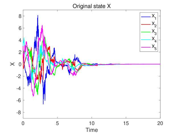
Figure 1: The trajectory $X$ running with the initial stabilizer $(K^{(0)},\widehat{K}^{(0)})$.

Following Algorithm 1, we update the policy to reinforce the target functions (28)-(29) to obtain $(P^{*},\widehat{P}^{*})$. From (53) and (55), we obtain

$$P^{*}=\begin{bmatrix}0.4152&0.3890&0.2068&0.0161&-0.4060\\ 0.3890&2.7211&1.9100&-2.6077&-0.7757\\ 0.2068&1.9100&1.8537&-1.8333&-0.8980\\ 0.0161&-2.6077&-1.8333&4.2409&-0.2664\\ -0.4060&-0.7757&-0.8980&-0.2664&2.1540\end{bmatrix},$$

and

$$\widehat{P}^{*}=\begin{bmatrix}0.6147&0.5721&0.2644&-0.1456&-0.6138\\ 0.5721&4.2583&2.8709&-4.4162&-0.6536\\ 0.2644&2.8709&2.6761&-2.6656&-1.0890\\ -0.1456&-4.4162&-2.6656&6.8164&-1.0676\\ -0.6138&-0.6536&-1.0890&-1.0676&3.1644\end{bmatrix}.$$

after 6 iterations for $P$ and 7 iterations for $\widehat{P}$.

To check whether $(P^{*},\widehat{P}^{*})$ is the solution of SAREs, we define

$$\left\{\begin{aligned} \mathcal{R}(P)&=A^{\top}P+PA+C^{\top}PC+Q-\big{(}PB+C^{\top}P+S^{\top}\big{)}\big{(}D^{\top}PD+R\big{)}^{-1}\big{(}B^{\top}P+D^{\top}PC+S\big{)},\\ \widehat{\mathcal{R}}(P,\widehat{P})&=\widehat{A}^{\top}\widehat{P}+\widehat{A}\widehat{P}+\widehat{C}^{\top}P\widehat{C}+\widehat{Q}-\big{(}\widehat{P}\widehat{B}+\widehat{C}^{\top}P\widehat{D}+\widehat{S}^{\top}\big{)}\big{(}\widehat{D}^{\top}P\widehat{D}+\widehat{R}\big{)}^{-1}\big{(}\widehat{B}^{\top}\widehat{P}+\widehat{D}^{\top}P\widehat{C}+\widehat{S}\big{)},\end{aligned}\right.$$

which are indeed the left sides of (11)-(12). Inserting $(P^{*},\widehat{P}^{*})$ into them, we obtain

$$\mathcal{R}(P^{*})=10^{-3}\cdot\begin{bmatrix}-0.2610&0.0466&0.0709&0.0414&0.0693\\ 0.0466&-0.0088&-0.0120&-0.0123&-0.0143\\ 0.0709&-0.0120&-0.0197&-0.0055&-0.0165\\ 0.0414&-0.0123&-0.0055&-0.0498&-0.0285\\ 0.0693&-0.0143&-0.0165&-0.0285&-0.0255\end{bmatrix},$$

and

$$\widehat{\mathcal{R}}(P^{*},\widehat{P}^{*})=10^{-7}\cdot\begin{bmatrix}-0.1213&0.0619&0.0734&0.0188&-0.0966\\ 0.0619&-0.0011&-0.0174&-0.0308&0.0401\\ 0.0734&-0.0174&0.2476&-0.0542&-0.1463\\ 0.0188&-0.0308&-0.0542&-0.0294&0.0817\\ -0.0966&0.0401&-0.1463&0.0817&0.0188\end{bmatrix}.$$

Also, the optimal control is $u^{*}=K\big{(}X^{*}-{\mathbb{E}_{t}}[X^{*}]\big{)}+\widehat{K}{\mathbb{E}_{t}}[X^{*}]$ with

$$K^{*}=\begin{bmatrix}-0.3575&0.0228&0.1682&-0.1102&-0.1300\\ 0.2188&0.6072&0.6793&-0.7718&-0.3158\end{bmatrix},$$

and

$$\widehat{K}^{*}=\begin{bmatrix}-0.3738&0.1098&0.2808&-0.0192&-0.1781\\ 0.1925&0.4796&0.6026&-0.6293&-0.2933\end{bmatrix}.$$

The optimal trajectory is shown in Figure 2.

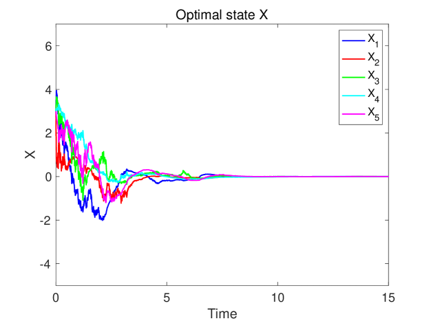
Figure 2: The trajectory $X$ running with the pre-commitment optimal control $u^{*}$.

Comparing the original state running with stabilizer $(K^{(0)},\widehat{K}^{(0)})$ to the optimal state with stabilizer $(K^{*},\widehat{K}^{*})$, we can see that the pre-commitment optimal trajectory converges to zero more quickly than the original state in Figure 1.

References

- [1] M. Ait Rami and X. Y. Zhou, “Linear matrix inequalities, Riccati equations, and indefinite stochastic linear quadratic controls”, IEEE Trans. Automat. Contr., vol. 45, pp. 1131-1143, 2000.
- [2] D. Andersson and B. Djehiche, “A maximum principle for SDEs of mean-field type”, Applied Mathematics and Optimization, vol. 63, pp. 341-356, 2011.
- [3] L. C. Baird, “Reinforcement learning in continuous time: Advantage updating,” in Proc. IEEE Int. Conf. Neural Netw., pp. 2448-2453, 1994.
- [4] S. J. Bradtke, B. E. Ydestie and A. G. Barto, “Adaptive linear quadratic control using policy iteration,” in Proc. Amer. Control Conf., pp. 3475-3476, 1994.
- [5] T. Bian, Y. Jiang and Z. P. Jiang, “Adaptive dynamic programming for stochastic systems with state and control dependent noise”, IEEE Trans. Automat. Contr., vol. 61, pp. 4170-4175, 2016.
- [6] S. J. Bradtke and M. O. Duff, “Reinforcement learning methods for continuous-time Markov decision problems”. In G. Tesauro, D. S. Touretzky, and T. K. Leen (Eds.), Advances in neural information processing systems, vol. 7 pp. 393-400. Cambridge, MA: MIT Press, 1995.
- [7] A. Bensoussan, J. Frehse and P. Yam, Mean Field Games and Mean Field Type Control Theory, SpringerBriefs in Mathematics, Springer, 2013.
- [8] R. Buckdahn, B. Djehiche and J. Li, “A general stochastic maximum principle for SDEs of mean-field type”, Applied Mathematics and Optimization, vol. 64, pp. 197-216, 2011.
- [9] X. Chen, G. Qu, Y. Tang, S. Low and N. Li, “Reinforcement learning for decision-making and control in power systems: Tutorial, review, and vision”, IEEE Trans. Smart Grid, to be published, doi: 10.1109/TSG.2022.3154718.
- [10] K. Du, Q. Meng and F. Zhang, “A Q-learning algorithm for discrete-time linear-quadratic control with random parameters of unknown distribution: convergence and stabilization”, vol. 60, pp.1991-2015, 2022.
- [11] R. Elliott, X. Li and Y. H. Ni, “Discrete time mean-field stochastic linear-quadratic optimal control problems”, Automatica, vol. 49, pp. 3222-3233, 2013.
- [12] W. Gao and Z. P. Jiang, “Learning-based adaptive optimal output regulation of linear and nonlinear systems: an overview”, Control Theory and Technology, vol. 20, pp. 1-19, 2022.
- [13] X. Gao, Z. Q. Xu and X. Y. Zhou, “State-dependent temperature control for Langevin diffusions”, SIAM J. Control Optimiz., vol. 60, pp. 1250-1268, 2022.
- [14] J. Huang, X. Li and J, Yong, “A Linear-quadratic optimal control problem for mean-field stochastic differential equations in infinite horizon”, Math. Control Relat. F., vol. 5, pp. 97-139, 2015.
- [15] M. Huang, P. E. Caines and Malhamé, R. P., “Large-population cost-coupled LQG problems with nonuniform agents: individual-mass behavior and decentralized -nash equilibria”, IEEE Transactions on Automatic Control, vol. 52(9), 1560–1571, 2007.
- [16] Y. Jia and X. Y. Zhou, “Policy evaluation and temporal-difference learning in continuous time and space: a martingale approach”, arXiv:2108.06655.
- [17] J. M. Lasry and P. L. Lions, “Mean field games”, JPN J. Math., vol. 2, pp. 229–260, 2007.
- [18] F. L. Lewis, D. Vrabie and K. G. Vamvoudakis, “Reinforcement learning and Feedback Control”, IEEE Contr. Syst. Mag., vol. 32, pp.76-105, 2012.
- [19] N. Li, X. Li, J. Peng and Z. Q. Xu, “Stochastic linear quadratic optimal control problem: A reinforcement learning method”, IEEE Trans. Automat. Contr., vol. 67, pp. 5009-5016, 2022.
- [20] N. Li, X. Li and Z. Yu, “Indefinite mean-field type linear–quadratic stochastic optimal control problems”, Automatica, vol. 122, 109267, 2020.
- [21] X. Li, J. Shi and J. Yong, “Mean-field linear-quadratic stochastic differential games in an infinite horizon”, ESAIM Contr. Optim. Ca, vol. 27, pp. 1-39, 2021.
- [22] Y. Li, Q. Song, F. Wu and G. Yin, “Solving a Class of Mean-Field LQG Problems”, IEEE Trans. Automat. Contr., Vol. 67, pp. 1579-1602, 2022.
- [23] Y. Lin, T. Zhang and W. Zhang, “Pareto-based guaranteed cost control of the uncertain mean-field stochastic systems in infinite horizon”, Automatica, vol. 92, pp. 197-209, 2018.
- [24] M. L. Minsky, “Theory of neural-analog reinforcement systems and its application to the brain model problem,” Ph.D. dissertation, Princeton University, 1954.
- [25] J. Moon and H. J. Yang, “Linear-quadratic time-inconsistent mean-field type Stackelberg differential games: time-consistent open-loop solutions”, IEEE Trans. Automat. Contr., vol. 66, pp. 375-382, 2021.
- [26] J. J. Murray, C. J. Cox, G. G. Lendaris and R. Saeks, “Adaptive dynamic programming”, IEEE T. Syst. Man Cy-S, vol. 32, pp. 140-153, 2002.
- [27] Y. H. Ni, R. Elliott and X. Li, “Discrete-time mean-field Stochastic linear–quadratic optimal control problems, II: Infinite horizon case”, Automatica, vol. 49, pp. 65-77, 2015.
- [28] B. Recht, “A Tour of Reinforcement Learning: The View from Continuous Control”, Annu. Rev. Contr. Robot, vol. 2, pp.253-279, 2019.
- [29] J. Sun, “Mean-field stochastic linear quadratic optimal control problems: Open-loop solvabilities”, ESAIM Contr. Optim. Ca., vol. 23, pp. 1099-1127, 2017.
- [30] R.S. Sutton, A.G. Barto, “Reinforcement learning: An introduction”, MIT Press, Cambridge, Second Edition, 2018.
- [31] R. Tian, Z. Yu and R. Zhang, “A closed-loop saddle point for zero-sum linear-quadratic stochastic differential games with mean-field type”, Syst. Control Lett., vol. 136, 104624, 2020.
- [32] H. Wang, T. Zariphopoulou and X. Y. Zhou, “Reinforcement learning in continuous time and space: A stochastic control approach”, Journal of Machine Learning Research, vol. 21, pp. 1-34, 2020.
- [33] H. Wang and X. Y. Zhou, “Continuous-time mean–variance portfolio selection: A reinforcement learning framework”, Mathematical Finance, vol. 30, pp. 1273-1308, 2020.
- [34] Y. Wang, Y. H. Ni, Z. Chen and J. F. Zhang, “Probabilistic framework of Howard’s policy iteration: BML evaluation and robust convergence analysis”, arXiv:2210.07473v1, 2022.
- [35] J. Yong, “Linear-Quadratic Optimal Control Problems for Mean-Field Stochastic Differential Equations”, SIAM J. Control Optimiz., vol. 51, pp. 2809-2838, 2013.
- [36] J. Yong, “Linear-Quadratic Optimal Control Problems for Mean-Field Stochastic Differential Equations-Time-Consistent solutions”, T. Am. Math. Soc., vol. 369, pp. 5467-5523, 2017.
- [37] J. Yong and X. Y. Zhou, Stochastic controls: Hamiltonian systems and HJB equations, Applications of Mathematics (New York), 43, Springer-Verlag, New York, 1999.
- [38] X. Y. Zhou and D. Li, “Continuous-Time Mean-Variance Portfolio Selection: A Stochastic LQ Framework”, Appl. Math. Optim., vol. 42, pp. 19-33, 2000.