Quaternion Matrix Completion Using Untrained Quaternion Convolutional Neural Network for Color Image Inpainting

Abstract

The use of quaternions as a novel tool for color image representation has yielded impressive results in color image processing. By considering the color image as a unified entity rather than separate color space components, quaternions can effectively exploit the strong correlation among the RGB channels, leading to enhanced performance. Especially, color image inpainting tasks are highly beneficial from the application of quaternion matrix completion techniques, in recent years. However, existing quaternion matrix completion methods suffer from two major drawbacks. First, it can be difficult to choose a regularizer that captures the common characteristics of natural images, and sometimes the regularizer that is chosen based on empirical evidence may not be the optimal or efficient option. Second, the optimization process of quaternion matrix completion models is quite challenging because of the non-commutativity of quaternion multiplication. To address the two drawbacks of the existing quaternion matrix completion approaches mentioned above, this paper tends to use an untrained quaternion convolutional neural network (QCNN) to directly generate the completed quaternion matrix. This approach replaces the explicit regularization term in the quaternion matrix completion model with an implicit prior that is learned by the QCNN. Extensive quantitative and qualitative evaluations demonstrate the superiority of the proposed method for color image inpainting compared with some existing quaternion-based and tensor-based methods.

1 Introduction

Color image inpainting is used to repair missing or damaged areas of a color image caused by sensor noise, compression artifacts, or other distortion. It can also restore color images with missing regions due to occlusions or other factors. In general, image inpainting can be used to improve the visual quality and completeness of images, and it is a useful tool for many fields including photography, film, and video production, as well as medical imaging and forensics.

Various methods have been proposed to address color image inpainting, with some of the popular ones including deep learning-based techniques [1, 2, 3], tensor completion methods [4, 5, 6, 7], and quaternion matrix completion methods [8, 9, 10, 11, 12]. These methods have been extensively researched and have shown significant improvement in the performance of color image inpainting tasks. Although deep learning-based methods often exhibit highly competitive results in color image inpainting, they still have some limitations in some cases. Firstly, training in deep learning methods requires a large amount of labeled data, which may be difficult to obtain in some scenarios. Secondly, deep learning methods often require a significant amount of computational resources and time for training and inference, which may be infeasible for resource-constrained applications that require fast image inpainting. Moreover, since deep learning methods are often trained based on specific data distributions [13], they may perform poorly under different data distributions. Therefore, non-deep learning methods based on tensor completion and quaternion matrix completion are highly popular in the application of color image inpainting due to their fast computation speed, good interpretability, and excellent performance on small datasets.

Although both third-order tensors and quaternion matrices can be used to represent color images, quaternion matrices, as a novel representation, have more reasonable characteristics and advantages in representing color images. When processing color pixels with RGB channels, third-order tensors may not be able to fully utilize the high correlation among the three channels. This is because the third-order tensors represent color images by simply stacking RGB channels together, which treats the relationship between the RGB channels (referred to as the ”intra-channel relationship”) and the relationship between pixels (referred to as the ”spatial relationship”) equally. Figure 1(a) shows the tensor perspective. Therefore, any unfolding (matrixization or vectorization) operation of the tensor can break this intra-channel relationship because it is not treated differently from the spatial relationship under the tensor perspective. By contrast, the quaternion always treats the three channels of color pixels as a whole [14, 9, 12], so it can preserve this intra-channel relationship well; see Figure 1(b), showing the quaternion perspective.

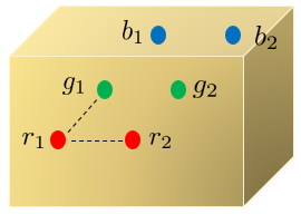
(a) Color pixels in tensor perspective.

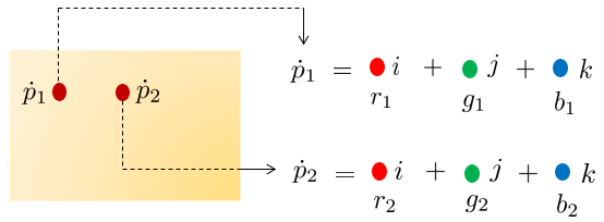
(b) Color pixels in quaternion perspective.

Figure 1: The difference between tensors and quaternions representing color pixels. $r_{m}$, $g_{m}$, and $b_{m}$ respectively denote the RGB channels of the color pixel $\mathbf{p}_{m}=(r_{m},g_{m},b_{m})$ under tensor perspective (or $\dot{p}_{m}=r_{m}i+g_{m}j+b_{m}k$ under quaternion perspective) for $m=1,2$. The relationship between pixels, e.g., $\mathbf{p}_{1}$ and $\mathbf{p}_{2}$ (or $\dot{p}_{1}$ and $\dot{p}_{2}$ in the quaternion matrix), is called “spatial relationship”, and the relationship between color channels is called “intra-channel relationship”. Under tensor perspective (a), the intra-channel and spatial relationships are obviously treated equally; that is, the relationship between $r_{1}$ and $g_{1}$ is the same as that between $r_{1}$ and $r_{2}$, which may not be appropriate. Under quaternion perspective (b), the three channels are always treated as a whole, and the intra-channel relationship (bundling with the three imaginary parts of a quaternion) is distinguished from the spatial relationship and can be maintained well.

Due to the superiority of quaternions in representing color pixels, quaternion matrix completion methods have recently achieved excellent results in color image inpainting. To complete quaternion matrices, there are primarily two approaches: minimizing the nuclear norm of the quaternion matrix [15, 8, 16] or decomposing the matrix into low-rank quaternion matrices [9, 12]. Nevertheless, currently available techniques for completing quaternion matrices have two notable limitations. Firstly, selecting an appropriate regularizer to capture the fundamental features of color images can be problematic, and in some cases, the selected regularizer (e.g. rank functions or total variation norm [17]) based on empirical observations may not be the most efficient or optimal. Secondly, the optimization process for quaternion matrix completion models is arduous due to the non-commutative nature of quaternion multiplication. Consequently, this paper aims to overcome the limitations of the current quaternion matrix completion methods mentioned above by utilizing an untrained quaternion convolutional neural network (QCNN) to produce the completed quaternion matrix directly. The proposed method has the following advantages: $1)$ Compared with traditional deep learning-based methods, our method directly exploits the deep priors of color images [18], and does not require a large amount of data to pre-train the network. $2)$ Using a network based on QCNN [19, 20, 21] to generate color images has advantages over traditional CNN, including prevention of overfitting, fewer parameters, and most importantly, the ability to fully simulate the inherent relationships between color image channels. A detailed explanation of QCNN can be found in Section 2.2. $3)$ This method will effectively avoid the limitations of existing quaternion matrix completion methods. Specifically, the QCNN learns an implicit prior that replaces the explicit regularization term in the quaternion matrix completion model, which will liberate researchers from the anguish of searching for suitable regularization terms and designing complex optimization algorithms for quaternion matrix completion models.

The remaining chapters of this paper are organized as follows: Section 2 introduces quaternions and QCNN. Section 3 provides details of the proposed color image inpainting approach. The qualitative and quantitative experiments are presented and analyzed in Section 4. Finally, some conclusions are drawn in Section 5.

2 Quaternions and Quaternion Convolutional Neural Network

In this section, we will provide a concise overview of quaternion algebra before delving into a thorough analysis of the key components that make up the QCNN.

2.1 Quaternion Algebra

As a natural extension of the complex domain, a quaternion $\dot{q}\in\mathbb{H}$ consisting of one real part and three imaginary parts is defined as

$$\dot{q}=\underbrace{q_{0}}_{{\rm{Re}}(\dot{q})}+\underbrace{q_{1}\texttt{i}+q_{2}\texttt{j}+q_{3}\texttt{k}}_{{\rm{Im}}(\dot{q})},$$ (1)

where $q_{l}\in\mathbb{R}\>(l=0,1,2,3)$, and $\texttt{i},\texttt{j},\texttt{k}$ are imaginary number units and obey the quaternion rules that

$$\left\{\begin{array}[]{lc}\texttt{i}^{2}=\texttt{j}^{2}=\texttt{k}^{2}=\texttt{i}\texttt{j}\texttt{k}=-1,\\ \texttt{i}\texttt{j}=-\texttt{j}\texttt{i}=\texttt{k},\texttt{j}\texttt{k}=-\texttt{k}\texttt{j}=\texttt{i},\texttt{k}\texttt{i}=-\texttt{i}\texttt{k}=\texttt{j}.\end{array}\right.$$

If the real part $q_{0}:={\rm{Re}}(\dot{q})=0$, then $\dot{q}=q_{1}\texttt{i}+q_{2}\texttt{j}+q_{3}\texttt{k}:={\rm{Im}}(\dot{q})$ is named a pure quaternion. The conjugate and the modulus of a quaternion $\dot{q}$ are, respectively, defined as

$$\dot{q}^{\ast}=q_{0}-q_{1}\texttt{i}-q_{2}\texttt{j}-q_{3}\texttt{k}\quad\text{and}\quad|\dot{q}|=\sqrt{q_{0}^{2}+q_{1}^{2}+q_{2}^{2}+q_{3}^{2}}.$$

Given two quaternions $\dot{p}$ and $\dot{q}\in\mathbb{H}$, the multiplication of them is

$$\begin{split}\dot{p}\dot{q}=&(p_{0}q_{0}-p_{1}q_{1}-p_{2}q_{2}-p_{3}q_{3})\\ &+(p_{0}q_{1}+p_{1}q_{0}+p_{2}q_{3}-p_{3}q_{2})\texttt{i}\\ &+(p_{0}q_{2}-p_{1}q_{3}+p_{2}q_{0}+p_{3}q_{1})\texttt{j}\\ &+(p_{0}q_{3}+p_{1}q_{2}-p_{2}q_{1}+p_{3}q_{0})\texttt{k},\end{split}$$ (2)

which is also referred to as Hamilton product [19]. Analogously, a quaternion matrix $\dot{\mathbf{Q}}=(\dot{q}_{mn})\in\mathbb{H}^{M\times N}$ is written as $\dot{\mathbf{Q}}=\mathbf{Q}_{0}+\mathbf{Q}_{1}\texttt{i}+\mathbf{Q}_{2}\texttt{j}+\mathbf{Q}_{3}\texttt{k}$, where $\mathbf{Q}_{l}\in\mathbb{R}^{M\times N}\>(l=0,1,2,3)$, $\dot{\mathbf{Q}}$ is named a pure quaternion matrix when $\mathbf{Q}_{0}={\rm{Re}}(\dot{\mathbf{Q}})=\mathbf{0}$.

2.2 Quaternion Convolutional Neural Networks

QCNN has quaternionic model parameters, inputs, activations, and outputs. In the following, we recall and analyze the key components used in this paper of QCNN, e.g., quaternion convolution, quaternion activation functions, and quaternion-valued backpropagation.

2.2.1 Quaternion Convolution

Convolution in the quaternion domain formally can be defined the same as that in the real domain [20, 22, 23]. Letting $\dot{\mathbf{K}}=(\dot{k}_{mn})=\mathbf{K}_{0}+\mathbf{K}_{1}\texttt{i}+\mathbf{K}_{2}\texttt{j}+\mathbf{K}_{3}\texttt{k}$ be a quaternion convolution kernel matrix, and $\dot{\mathbf{Y}}=(\dot{y}_{mn})=\mathbf{Y}_{0}+\mathbf{Y}_{1}\texttt{i}+\mathbf{Y}_{2}\texttt{j}+\mathbf{Y}_{3}\texttt{k}$ be a quaternion input matrix, their convolution in deep learning is computed as

$$(\dot{\mathbf{K}}\circledast\dot{\mathbf{Y}})(r_{1},r_{2})=\sum_{m}\sum_{n}\dot{k}_{mn}\dot{y}_{r_{1}+m,r_{2}+n},$$ (3)

where $\circledast$ denotes convolution operation. Deconvolution, strided convolution, dilated convolution, and padding in quaternion domain are also defined analogously to real-valued convolution. Assume that $\dot{\mathbf{X}}=\mathbf{X}_{0}+\mathbf{X}_{1}\texttt{i}+\mathbf{X}_{2}\texttt{j}+\mathbf{X}_{3}\texttt{k}$ is a certain window (patch) of $\dot{\mathbf{Y}}$, and has the same size as $\dot{\mathbf{K}}$. Based on the Hamilton product (2), the convolution of $\dot{\mathbf{K}}$ and $\dot{\mathbf{X}}$ can be written as

$$\begin{split}\dot{\mathbf{K}}\circledast\dot{\mathbf{X}}=&(\mathbf{K}_{0}\circledast\mathbf{X}_{0}-\mathbf{K}_{1}\circledast\mathbf{X}_{1}-\mathbf{K}_{2}\circledast\mathbf{X}_{2}-\mathbf{K}_{3}\circledast\mathbf{X}_{3})\\ &+(\mathbf{K}_{0}\circledast\mathbf{X}_{1}+\mathbf{K}_{1}\circledast\mathbf{X}_{0}+\mathbf{K}_{2}\circledast\mathbf{X}_{3}-\mathbf{K}_{3}\circledast\mathbf{X}_{2})\texttt{i}\\ &+(\mathbf{K}_{0}\circledast\mathbf{X}_{2}-\mathbf{K}_{1}\circledast\mathbf{X}_{3}+\mathbf{K}_{2}\circledast\mathbf{X}_{0}+\mathbf{K}_{3}\circledast\mathbf{X}_{1})\texttt{j}\\ &+(\mathbf{K}_{0}\circledast\mathbf{X}_{3}+\mathbf{K}_{1}\circledast\mathbf{X}_{2}-\mathbf{K}_{2}\circledast\mathbf{X}_{1}+\mathbf{K}_{3}\circledast\mathbf{X}_{0})\texttt{k}.\end{split}$$ (4)

From (4), one can see that if $\dot{\mathbf{X}}$ and $\dot{\mathbf{K}}$ are real-valued matrices, i.e., $\mathbf{X}_{1}=\mathbf{X}_{2}=\mathbf{X}_{3}=\mathbf{K}_{1}=\mathbf{K}_{2}=\mathbf{K}_{3}=\mathbf{0}$, then the convolution degrades into the traditional real-valued case. Labeling $\dot{\mathbf{K}}\circledast\dot{\mathbf{X}}={\rm{Re}}(\dot{\mathbf{K}}\circledast\dot{\mathbf{X}})+{\rm{Im}}_{1}(\dot{\mathbf{K}}\circledast\dot{\mathbf{X}})\texttt{i}+{\rm{Im}}_{2}(\dot{\mathbf{K}}\circledast\dot{\mathbf{X}})\texttt{j}+{\rm{Im}}_{3}(\dot{\mathbf{K}}\circledast\dot{\mathbf{X}})\texttt{k}$, and using a matrix to represent the components of the convolution, we express the quaternion convolution formula (4) in the following way similar to matrix multiplication:

$$\begin{bmatrix}{\rm{Re}}(\dot{\mathbf{K}}\circledast\dot{\mathbf{X}})\\ {\rm{Im}}_{1}(\dot{\mathbf{K}}\circledast\dot{\mathbf{X}})\\ {\rm{Im}}_{2}(\dot{\mathbf{K}}\circledast\dot{\mathbf{X}})\\ {\rm{Im}}_{3}(\dot{\mathbf{K}}\circledast\dot{\mathbf{X}})\end{bmatrix}=\begin{bmatrix}\mathbf{K}_{0}&-\mathbf{K}_{1}&-\mathbf{K}_{2}&-\mathbf{K}_{3}\\ \mathbf{K}_{1}&\mathbf{K}_{0}&-\mathbf{K}_{3}&\mathbf{K}_{2}\\ \mathbf{K}_{2}&\mathbf{K}_{3}&\mathbf{K}_{0}&-\mathbf{K}_{1}\\ \mathbf{K}_{3}&-\mathbf{K}_{2}&\mathbf{K}_{1}&\mathbf{K}_{0}\end{bmatrix}\circledast\begin{bmatrix}\mathbf{X}_{0}\\ \mathbf{X}_{1}\\ \mathbf{X}_{2}\\ \mathbf{X}_{3}\end{bmatrix}.$$ (5)

In addition, one can visually see the differences between real-valued convolution and quaternion convolution in Figure 2. From formula (5) and Figure 2, we can notice that the quaternion convolution forces each component of the quaternion kernel $\dot{\mathbf{K}}$ to interact with each component of the input quaternion feature map $\dot{\mathbf{X}}$. This kind of interaction mechanism forces the kernel to capture internal latent relations among different channels of the feature map since each characteristic in a channel will have an influence on the other channels through the common kernel. Different from real-valued convolution, which simply multiplies each kernel with the corresponding feature map, the quaternion convolution is similar to a mixture of standard convolution. Such a mixture can perfectly simulate the potential relationship between color image channels. This may be the fundamental reason why QCNN is more suitable for generating color images. No real-valued CNN would make such connections without the inspiration from quaternion convolutions, although it is feasible to incorporate this mixture into three real-valued CNNs using supplementary connections. Furthermore, when the quaternion convolution layer has the same output dimensions (a quaternion has four dimensions) as the real-valued convolution layer, for the quaternion convolution, the parameters that need to be learned are only $\frac{1}{4}$ of the real-valued convolution, which has great potential to avoid the over-fitting phenomenon. These exciting characteristics of quaternion convolution are our main motivation for designing QCNN to color image inpainting tasks.

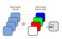
(a) Real-valued convolution

(b) Quaternion convolution

Figure 2: The differences between (a) real-valued convolution and (b) quaternion convolution.

2.2.2 Quaternion activation functions

Many quaternion activation functions have been investigated, whereas the split activation [19, 24], a more frequent and simpler solution, is applied in our proposed model. Let $Q_{\mathfrak{f}}(\dot{\mathbf{Y}})$ be a split activation function applied to the quaternion $\dot{\mathbf{Y}}=\mathbf{Y}_{0}+\mathbf{Y}_{1}\texttt{i}+\mathbf{Y}_{2}\texttt{j}+\mathbf{Y}_{3}\texttt{k}$, such that

$$Q_{\mathfrak{f}}(\dot{\mathbf{Y}})=\mathfrak{f}(\mathbf{Y}_{0})+\mathfrak{f}(\mathbf{Y}_{1})\texttt{i}+\mathfrak{f}(\mathbf{Y}_{2})\texttt{j}+\mathfrak{f}(\mathbf{Y}_{3})\texttt{k},$$

with $\mathfrak{f}$ corresponding to any traditional real-valued activation function, e.g., ReLU, LeakyReLU, sigmoid, etc. Thus, $Q_{\mathfrak{f}}$ can be, $Q_{ReLU}$, $Q_{LeakyReLU}$, $Q_{sigmoid}$, $Q_{Tanh}$, etc.

2.2.3 Quaternion-Valued Backpropagation

The quaternion-valued backpropagation is just an extension of the method for its real-valued counterpart [19]. The gradient of a general quaternion loss function $\mathcal{L}$ is computed for each component of the quaternion kernel matrix $\dot{\mathbf{K}}$ as

$$\frac{\nabla\mathcal{L}}{\nabla\dot{\mathbf{K}}}=\frac{\nabla\mathcal{L}}{\nabla\mathbf{K}_{0}}+\frac{\nabla\mathcal{L}}{\nabla\mathbf{K}_{1}}\texttt{i}+\frac{\nabla\mathcal{L}}{\nabla\mathbf{K}_{2}}\texttt{j}+\frac{\nabla\mathcal{L}}{\nabla\mathbf{K}_{3}}\texttt{k},$$

where $\nabla$ denotes gradient operator. Afterwards, the gradient is propagated back based on the chain rule. Thus, QCNN can be easily trained as real-valued CNN following the backpropagation.

3 Color Image Inpainting

As quaternions offer a superior method of representing color pixels, every pixel in an RGB color image can be encoded as a pure quaternion. That is

$$\dot{q}=0+q_{r}\texttt{i}+q_{g}\texttt{j}+q_{b}\texttt{k},$$ (6)

where $\dot{q}$ denotes a color pixel, $q_{r}$, $q_{g}$, and $q_{b}$ are respectively the pixel values in red, green, and blue channels. Naturally, the given color image with spatial resolution of $M\times N$ pixels can be represented by a pure quaternion matrix $\dot{\mathbf{Q}}=(\dot{q}_{mn})\in\mathbb{H}^{M\times N}$, $1\leq m\leq M$, $1\leq n\leq N$ as follows:

$$\dot{\mathbf{Q}}=\mathbf{0}+\mathbf{Q}_{r}\texttt{i}+\mathbf{Q}_{g}\texttt{j}+\mathbf{Q}_{b}\texttt{k},$$ (7)

where $\mathbf{Q}_{r},\mathbf{Q}_{g},\mathbf{Q}_{b}\in\mathbb{R}^{M\times N}$ containing respectively the pixel values in red, green, and blue channels. Figure 3 shows an example of using a quaternion matrix to represent a color image.

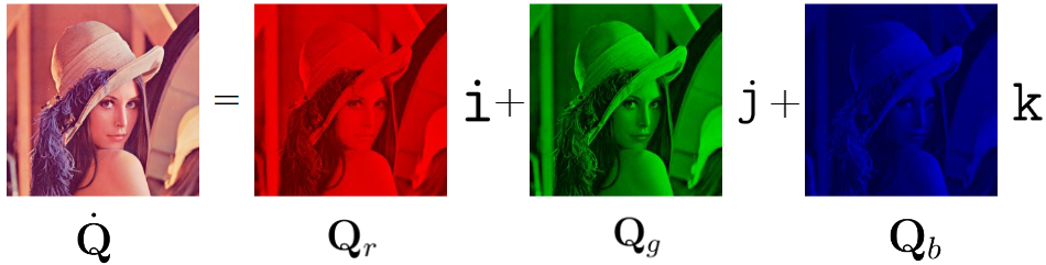
Figure 3: Color image represented by quaternion matrix.

3.1 Optimization Model

In the quaternion domain, a general quaternion matrix completion model for color image inpainting can be developed as

$$\mathop{{\rm{min}}}\limits_{\dot{\mathbf{X}}}\ \frac{1}{2}\|\mathcal{P}_{\Omega}(\dot{\mathbf{X}}-\dot{\mathbf{Q}})\|_{F}^{2}+\lambda\Phi(\dot{\mathbf{X}}),$$ (8)

where $\lambda$ is a nonnegative parameter, $\dot{\mathbf{X}}\in\mathbb{H}^{M\times N}$ is a desired output completed quaternion matrix, $\dot{\mathbf{Q}}\in\mathbb{H}^{M\times N}$ is an observed quaternion matrix with missing entries, $\Phi(\cdot)$ is a regularization operator, and $\mathcal{P}_{\Omega}$ is the unitary projection onto the linear space of matrices supported on the entries set $\Omega$, defined as

$$(\mathcal{P}_{\Omega}(\dot{\mathbf{X}}))_{mn}=\left\{\begin{array}[]{c}\!\!\!\dot{x}_{mn},\qquad(m,n)\in\Omega,\\ 0,\qquad\quad\>(m,n)\notin\Omega.\end{array}\right.$$

In model (8), $\Phi(\cdot)$ can be the rank function, as used in recent quaternion matrix completion models [15, 25, 26], or any other suitable regularizer, or a combination of them. However, selecting an appropriate regularizer to capture the generic prior of natural images can be challenging, and in some cases, the empirically chosen regularizer may not be the most suitable or effective one. Furthermore, optimizing regularizers in the quaternion domain is a challenging task because of the non-commutativity of quaternion multiplication. Thus, in this paper, we propose to replace the explicit regularization term $\Phi(\cdot)$ with an implicit prior learned by the QCNN. As a result, the model (8) becomes

$$\mathop{{\rm{min}}}\limits_{\dot{\mathbf{\theta}}}\ \|\mathcal{P}_{\Omega}(f_{\dot{\mathbf{\theta}}}(\dot{\mathbf{Z}})-\dot{\mathbf{Q}})\|_{F}^{2},\quad\text{and}\quad\dot{\mathbf{X}}_{opt}=f_{\dot{\mathbf{\theta}}_{opt}}(\dot{\mathbf{Z}}),$$ (9)

where $\dot{\mathbf{Z}}$, a random initialization with the same size as $\dot{\mathbf{Q}}$, is passed as input to the QCNN $f_{\dot{\mathbf{\theta}}}(\dot{\mathbf{Z}})$ which is parameterized by $\dot{\mathbf{\theta}}$. Since there should not be any change in the uncorrupted regions, the final output pixels outside of the corrupted areas are replaced with the original input values. Therefore, once we get $\dot{\mathbf{X}}_{opt}$, the final inpainted color image is

$$\dot{\mathbf{X}}_{inpainted}=\mathcal{P}_{\Omega}(\dot{\mathbf{Q}})+\mathcal{P}_{\Omega^{c}}(\dot{\mathbf{X}}_{opt}),$$ (10)

where $\Omega^{c}$ is the complement of $\Omega$.

3.2 The Designed QCNN

The designed QCNN is an encoder-decoder, which includes an encoding part with four times downsampling and a decoding part with four quaternion deconvolution (Qdeconv) layers for backing to the original size of the color image. The architecture and details of the designed QCNN can be seen in Figure 4 and Table 1, respectively. The quaternion batch normalization (QBN) method studied in [20, 27] is also used in the designed QCNN to stabilize and speed up the process of generating the quaternion matrix $\dot{\mathbf{X}}_{opt}$.

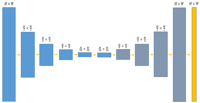
Figure 4: The architecture of the designed QCNN.

Table 1: The details of the designed QCNN.

Module types	Kernel size	Stride	Output channels
Qconv+QBN+$Q_{LeakyReLU}$	$3\times 3$	$1\times 1$	$64$
Qconv+QBN+$Q_{LeakyReLU}$	$3\times 3$	$2\times 2$	$64$
Qconv+QBN+$Q_{LeakyReLU}$	$3\times 3$	$2\times 2$	$64$
Qconv+QBN+$Q_{LeakyReLU}$	$3\times 3$	$2\times 2$	$64$
Qconv+QBN+$Q_{LeakyReLU}$	$3\times 3$	$2\times 2$	$64$
Qconv+QBN+$Q_{LeakyReLU}$	$3\times 3$	$1\times 1$	$64$
Qdeconv+QBN+$Q_{LeakyReLU}$	$3\times 3$	$2\times 2$	$64$
Qdeconv+QBN+$Q_{LeakyReLU}$	$3\times 3$	$2\times 2$	$64$
Qdeconv+QBN+$Q_{LeakyReLU}$	$3\times 3$	$2\times 2$	$64$
Qdeconv+QBN+$Q_{LeakyReLU}$	$3\times 3$	$2\times 2$	$64$
Qconv	$3\times 3$	$1\times 1$	$1$

4 Experiments

4.1 Experiment Settings

The experiments for our proposed QCNN-based method for color image inpainting were conducted in an environment with “torch==1.13.1+cu116”. During backpropagation, we have chosen the Adam optimizer with a learning rate of 0.01. In addition, the input of the QCNN, $\dot{\mathbf{Z}}$, is a random quaternion matrix with the same spatial size as the color image to be inpainted. The output of the QCNN is a completed quaternion matrix whose imaginary parts correspond to the inpainted RGB color image.

4.2 Datasets

We evaluate the proposed method on eight common-used color images (including “baboon”, “monarch”, “airplane”, “peppers”, “sailboat”, “lena”, “panda”, and “barbara”, see Figure 5) with spatial size $256\times 256$.

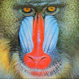
(a) baboon

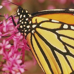
(b) monarch

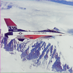
(c) airplane

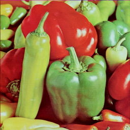
(d) peppers

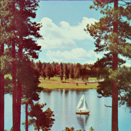
(e) sailboat

(f) lena

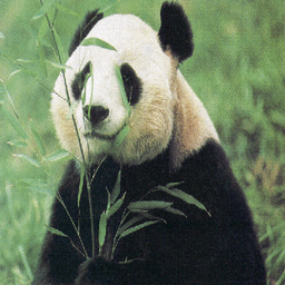
(g) panda

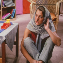
(h) barbara

Figure 5: Tested color images.

For random missing, we set three levels of sampling rates (SRs) which are ${\rm{SR}}=10\%$, ${\rm{SR}}=30\%$, and ${\rm{SR}}=50\%$. For structural missing, we use two kinds of cases, see the observed color images in Figure 10.

4.3 Comparison

We compare our QCNN-based method with its real-domain counterpart, i.e., the CNN-based method with the same number of learnable parameters as our model. Additionally, we compare our method with several well-known tensor and quaternion-based techniques that utilize low-rank regularization, namely t-SVD [28], TMac-TT [29], LRQA-2 [15], LRQMC [9], and TQLNA [30]. The implementation of all the comparison methods follow their original papers and source codes. For measuring the quality of the results, two metrics, peak signal-to-noise ratio (PSNR) and structure similarity index (SSIM) [31] are used in this paper.

Table 2: The PSNR and SSIM values of different methods on the eight color images with three levels of sampling rates (the format is PSNR/SSIM, and bold fonts denote the best performance).

Methods:	CNN	t-SVD [28]	TMac-TT [29]	LRQA-2 [15]	LRQMC [9]	TQLNA [30]	Ours
Images:	${\rm{SR}}=10\%$
baboon	18.456/0.572	17.325/0.505	19.242/0.579	17.941/0.527	18.065/0.546	18.075/0.537	20.301/0.647
monarch	19.589/0.860	17.325/0.643	17.306/0.763	14.561/0.642	14.752/0.684	13.534/0.579	20.292/0.874
airplane	21.001/0.675	17.765/0.377	20.503/0.588	18.601/0.424	18.715/0.480	18.442/0.416	22.258/0.715
peppers	23.328/0.929	15.993/0.718	20.416/0.871	17.111/0.761	16.206/0.740	17.145/0.764	23.672/0.932
sailboat	20.018/0.781	16.514/0.502	17.606/0.670	17.103/0.550	17.295/0.581	16.711/0.526	20.714/0.785
lena	22.773/0.913	17.659/0.798	21.616/0.877	18.607/0.811	18.553/0.825	18.528/0.802	23.724/0.925
panda	23.399/0.695	18.074/0.492	22.518/0.628	19.205/0.514	19.212/0.562	19.149/0.513	24.408/0.764
barbara	21.524/0.754	16.894/0.513	20.373/0.723	17.917/0.533	17.947/0.585	17.996/0.527	22.943/0.783
Images:	${\rm{SR}}=30\%$
baboon	21.800/0.761	20.657/0.703	21.801/0.751	20.685/0.695	21.279/0.727	20.878/0.705	22.565/0.775
monarch	25.163/0.950	19.003/0.833	22.487/0.910	19.582/0.842	19.725/0.851	19.876/0.848	25.278/0.952
airplane	25.301/0.843	22.555/0.671	24.096/0.821	22.982/0.681	23.183/0.724	23.250/0.702	26.119/0.852
peppers	28.281/0.973	22.287/0.908	25.458/0.951	23.330/0.923	23.671/0.930	23.976/0.934	28.536/0.976
sailboat	24.374/0.904	20.958/0.767	22.819/0.862	21.343/0.779	21.634/0.806	21.609/0.792	24.723/0.906
lena	27.519/0.963	23.217/0.917	26.136/0.951	23.729/0.921	24.173/0.931	24.059/0.927	27.730/0.966
panda	27.416/0.850	23.698/0.730	26.602/0.837	24.297/0.739	24.479/0.772	24.721/0.753	27.828/0.862
barbara	25.804/0.875	22.737/0.771	25.338/0.866	23.403/0.781	23.584/0.799	23.885/0.797	26.550/0.883
Images:	${\rm{SR}}=50\%$
baboon	24.263/0.858	21.837/0.764	23.547/0.839	23.004/0.812	23.704/0.839	23.099/0.816	24.588/0.865
monarch	28.834/0.976	23.558/0.927	26.256/0.957	24.089/0.932	24.079/0.935	24.587/0.938	29.015/0.977
airplane	29.525/0.928	26.626/0.835	28.217/0.922	26.768/0.822	27.195/0.869	27.438/0.850	29.705/0.931
peppers	31.622/0.987	27.287/0.966	29.461/0.980	27.936/0.971	28.171/0.973	28.749/0.976	31.675/0.989
sailboat	27.541/0.950	24.723/0.890	26.251/0.932	25.000/0.892	25.525/0.910	25.414/0.902	27.816/0.953
lena	30.749/0.980	27.385/0.962	29.360/0.975	27.476/0.962	28.189/0.968	28.128/0.967	30.991/0.982
panda	30.414/0.914	27.746/0.856	29.458/0.905	27.985/0.853	28.438/0.880	28.438/0.865	30.548/0.916
barbara	28.259/0.924	26.838/0.884	27.836/0.918	27.252/0.888	27.891/0.905	27.719/0.897	29.041/0.931

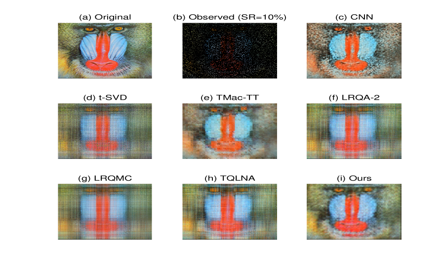
(a) baboon

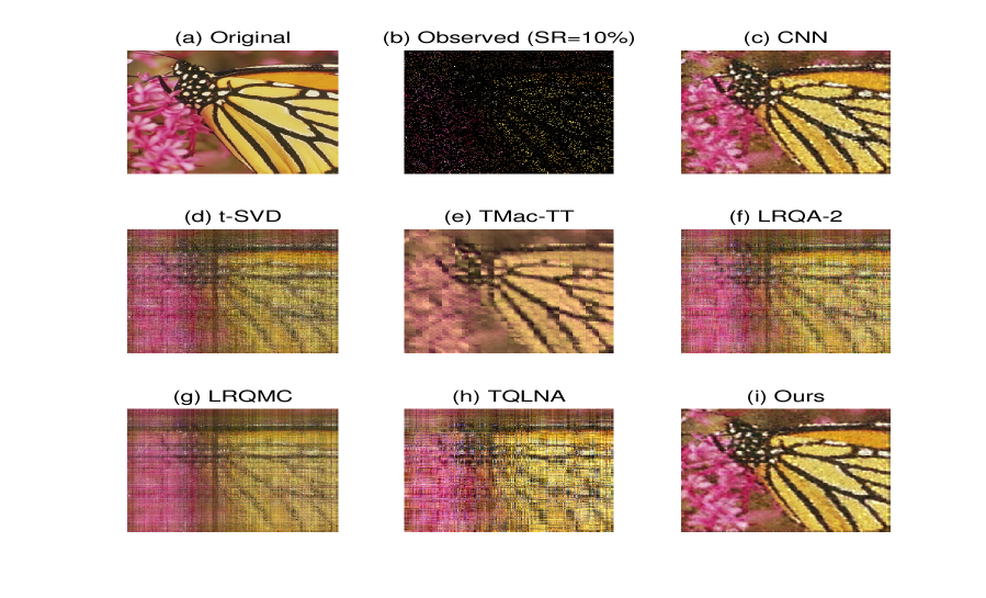
(b) monarch

Figure 6: Recovered two color images (baboon and monarch) for random missing with ${\rm{SR}}=10\%$.

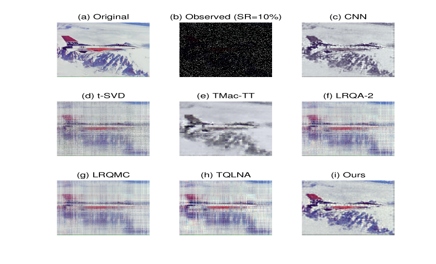
(a) airplane

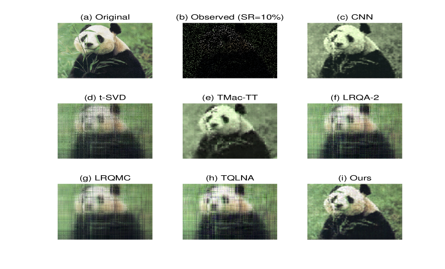
(b) panda

Figure 7: Recovered two color images (airplane and panda) for random missing with ${\rm{SR}}=10\%$.

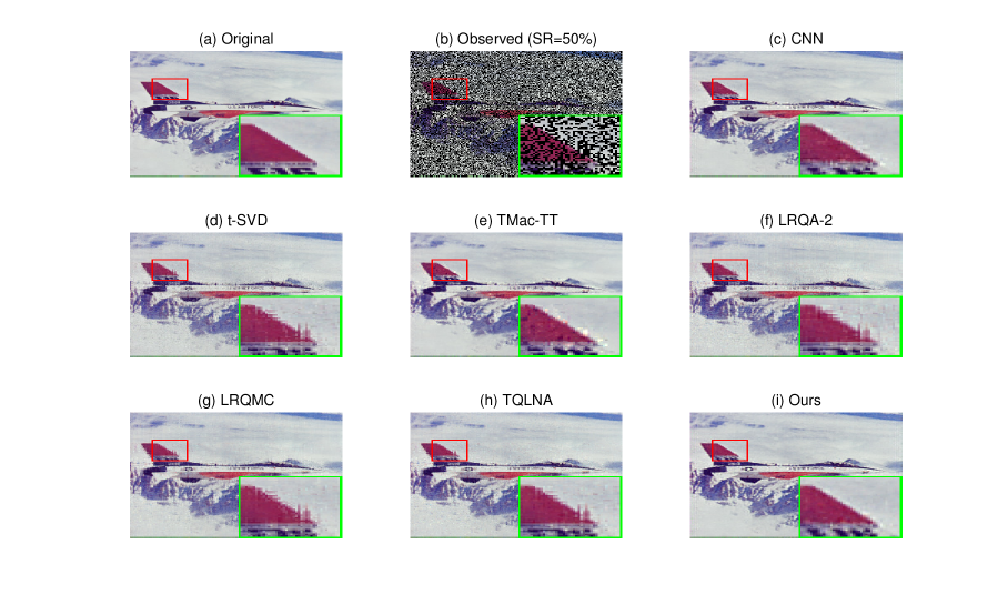
(a) airplane

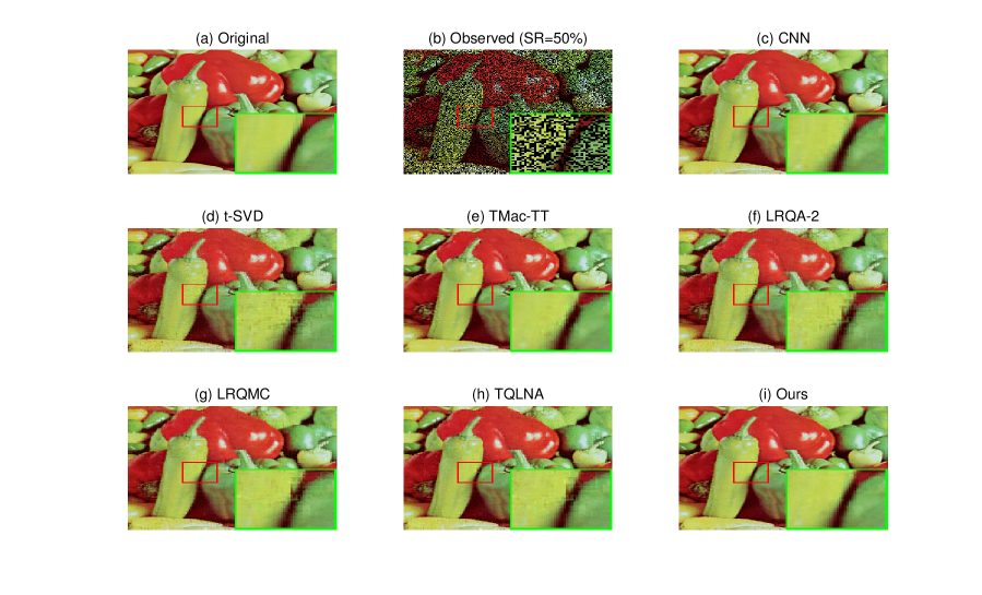
(b) peppers

Figure 8: Recovered two color images (airplane and peppers) for random missing with ${\rm{SR}}=50\%$.

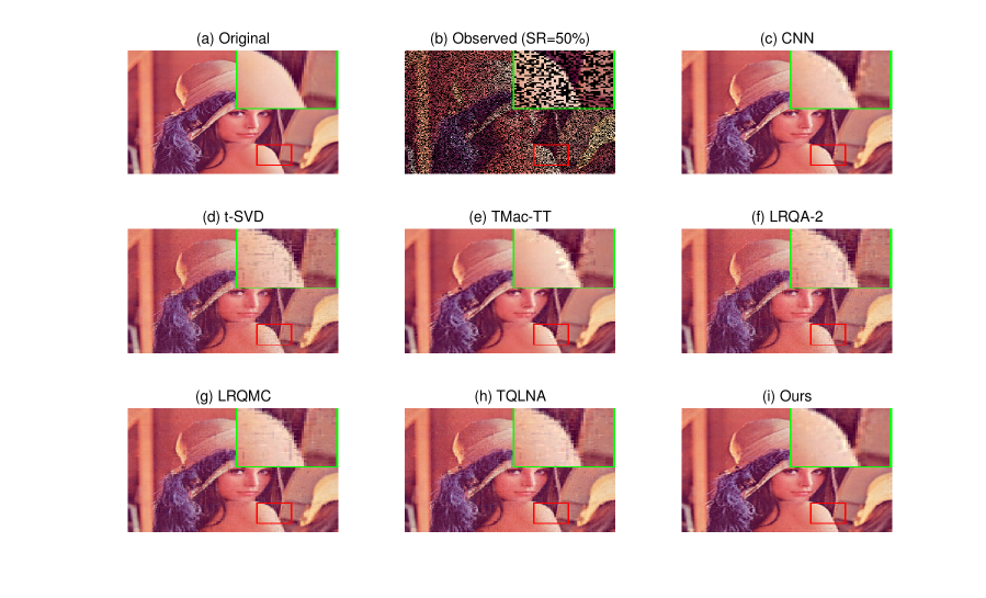
(a) lena

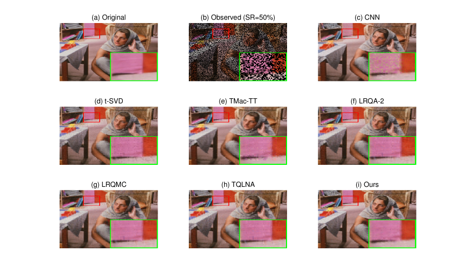
(b) barbara

Figure 9: Recovered two color images (lena and barbara) for random missing with ${\rm{SR}}=50\%$.

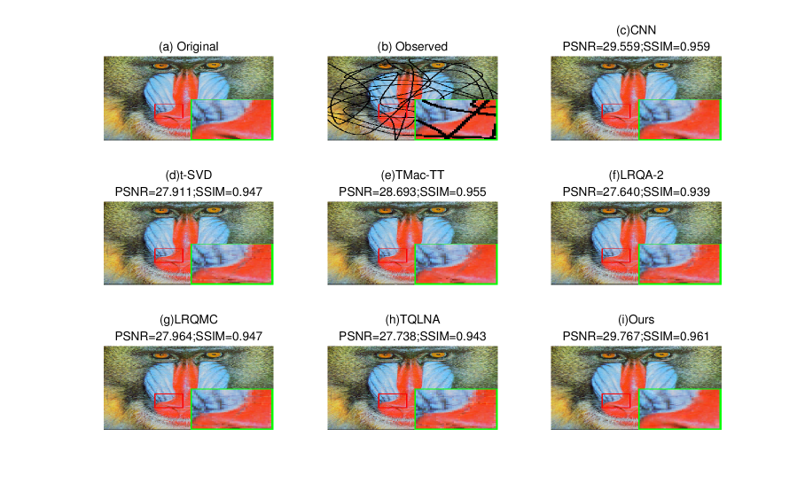
(a) baboon

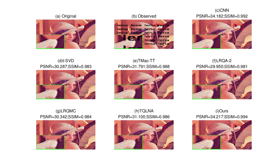
(b) lena

Figure 10: Recovered two color images (baboon and lena) for structural missing pixels.

4.4 Results Analysis

Table 2 lists the PSNR and SSIM values of different methods on the eight color images with three levels of sampling rates. Figure 6 and Figure 7 display the recovered results of four color images by different methods for random missing with ${\rm{SR}}=10\%$. Figure 8 and Figure 9 display the recovered results of four color images by different methods for random missing with ${\rm{SR}}=50\%$. Experimental results of two kinds of structural missing cases are given in Figure 10. From all the experimental results, we can observe and summarize the following points:

• Our QCNN-based color image inpainting method has advantages over the CNN-based method, especially in the case of a large number of lost pixels (e.g., SR=10%), the advantages of our QCNN-based method are obvious. As shown in Figures 6 and 7, when SR=10%, the color images generated by the CNN-based method shows an obvious color difference compared with the original images. In addition, our QCNN-based method has advantages over CNN-based methods in preserving color image details (see Figures 8 and 9). The QCNN-based method has advantages over the CNN-based method mainly because the CNN-based method, for each kernel, simply merges the RGB three channels to sum the convolution results up, without considering the complicated interrelationship between different channels. This may result in the loss of important structural information.

• Compared with existing methods based on low-rank approximation of quaternion matrices, our QCNN-based method replaced the explicit regularization term with an implicit prior learned by the QCNN. Therefore, our QCNN-based method has obvious advantages over the existing methods based on quaternion matrix low-rank approximation, both in terms of evaluation indicators and visually (see Table 2 and Figures 6-10).

5 Conclusion

For color image inpainting, this paper has proposed a quaternion matrix completion method using untrained QCNN. This approach enhances the quaternion matrix completion model by substituting the explicit regularization term with an implicit prior, which is acquired through learning by the QCNN. This method eliminates the need for researchers to spend time searching for appropriate regularization terms and designing intricate optimization algorithms for quaternion matrix completion models. From the experimental results, it can be seen that the method is very competitive with the existing quaternion matrix completion methods in the task of color image inpainting.

This paper represents the first attempt to apply QCNN to the quaternion matrix completion problem, and may therefore provide new insights for researchers exploring quaternion matrix completion methods, as well as other quaternion matrix optimization problems.

References

- [1] Tao Yu, Zongyu Guo, Xin Jin, Shilin Wu, Zhibo Chen, Weiping Li, Zhizheng Zhang, and Sen Liu. Region normalization for image inpainting. In Proceedings of the AAAI conference on artificial intelligence, volume 34, pages 12733–12740, 2020.
- [2] Weize Quan, Ruisong Zhang, Yong Zhang, Zhifeng Li, Jue Wang, and Dong-Ming Yan. Image inpainting with local and global refinement. IEEE Transactions on Image Processing, 31:2405–2420, 2022.
- [3] Cai Ran, Xinfu Li, and Fang Yang. Multi-step structure image inpainting model with attention mechanism. Sensors, 23(4):2316, 2023.
- [4] Wenjin Qin, Hailin Wang, Feng Zhang, Jianjun Wang, Xin Luo, and Tingwen Huang. Low-rank high-order tensor completion with applications in visual data. IEEE Transactions on Image Processing, 31:2433–2448, 2022.
- [5] Hongjin He, Chen Ling, and Wenhui Xie. Tensor completion via a generalized transformed tensor t-product decomposition without t-svd. Journal of Scientific Computing, 93(2):47, 2022.
- [6] Yu-Bang Zheng, Ting-Zhu Huang, Teng-Yu Ji, Xi-Le Zhao, Tai-Xiang Jiang, and Tian-Hui Ma. Low-rank tensor completion via smooth matrix factorization. Applied Mathematical Modelling, 70:677–695, 2019.
- [7] Ben-Zheng Li, Xi-Le Zhao, Jian-Li Wang, Yong Chen, Tai-Xiang Jiang, and Jun Liu. Tensor completion via collaborative sparse and low-rank transforms. IEEE Transactions on Computational Imaging, 7:1289–1303, 2021.
- [8] Zhigang Jia, Michael K Ng, and Guang-Jing Song. Robust quaternion matrix completion with applications to image inpainting. Numerical Linear Algebra with Applications, 26(4):e2245, 2019.
- [9] Jifei Miao and Kit Ian Kou. Color image recovery using low-rank quaternion matrix completion algorithm. IEEE Transactions on Image Processing, 31:190–201, 2021.
- [10] Junren Chen and Michael K Ng. Color image inpainting via robust pure quaternion matrix completion: Error bound and weighted loss. SIAM Journal on Imaging Sciences, 15(3):1469–1498, 2022.
- [11] Zhigang Jia, Qiyu Jin, Michael K Ng, and Xi-Le Zhao. Non-local robust quaternion matrix completion for large-scale color image and video inpainting. IEEE Transactions on Image Processing, 31:3868–3883, 2022.
- [12] Jifei Miao and Kit Ian Kou. Quaternion-based bilinear factor matrix norm minimization for color image inpainting. IEEE Transactions on Signal Processing, 68:5617–5631, 2020.
- [13] Yoshua Bengio, Aaron Courville, and Pascal Vincent. Representation learning: A review and new perspectives. IEEE transactions on pattern analysis and machine intelligence, 35(8):1798–1828, 2013.
- [14] Jifei Miao, Kit Ian Kou, and Wankai Liu. Low-rank quaternion tensor completion for recovering color videos and images. Pattern Recognition, 107:107505, 2020.
- [15] Yongyong Chen, Xiaolin Xiao, and Yicong Zhou. Low-rank quaternion approximation for color image processing. IEEE Transactions on Image Processing, 29:1426–1439, 2019.
- [16] Chaoyan Huang, Zhi Li, Yubing Liu, Tingting Wu, and Tieyong Zeng. Quaternion-based weighted nuclear norm minimization for color image restoration. Pattern Recognition, 128:108665, 2022.
- [17] Zhigang Jia, Michael K Ng, and Wei Wang. Color image restoration by saturation-value total variation. SIAM Journal on Imaging Sciences, 12(2):972–1000, 2019.
- [18] Dmitry Ulyanov, Andrea Vedaldi, and Victor Lempitsky. Deep image prior. In Proceedings of the IEEE conference on computer vision and pattern recognition, pages 9446–9454, 2018.
- [19] Titouan Parcollet, Mohamed Morchid, and Georges Linarès. A survey of quaternion neural networks. Artificial Intelligence Review, 53:2957–2982, 2020.
- [20] Chase J Gaudet and Anthony S Maida. Deep quaternion networks. In 2018 International Joint Conference on Neural Networks (IJCNN), pages 1–8. IEEE, 2018.
- [21] Titouan Parcollet, Mirco Ravanelli, Mohamed Morchid, Georges Linarès, Chiheb Trabelsi, Renato De Mori, and Yoshua Bengio. Quaternion recurrent neural networks. arXiv preprint arXiv:1806.04418, 2018.
- [22] Titouan Parcollet, Ying Zhang, Mohamed Morchid, Chiheb Trabelsi, Georges Linarès, Renato de Mori, and Yoshua Bengio. Quaternion convolutional neural networks for end-to-end automatic speech recognition. In Interspeech 2018, 19th Annual Conference of the International Speech Communication Association, Hyderabad, India, 2-6 September 2018, pages 22–26. ISCA, 2018.
- [23] Yu Zhou, Lianghai Jin, Hong Liu, and Enmin Song. Color facial expression recognition by quaternion convolutional neural network with gabor attention. IEEE Transactions on Cognitive and Developmental Systems, 13(4):969–983, 2020.
- [24] Titouan Parcollet, Mohamed Morchid, and Georges Linares. Deep quaternion neural networks for spoken language understanding. In 2017 IEEE Automatic Speech Recognition and Understanding Workshop (ASRU), pages 504–511. IEEE, 2017.
- [25] Guangjing Song, Weiyang Ding, and Michael K Ng. Low rank pure quaternion approximation for pure quaternion matrices. SIAM Journal on Matrix Analysis and Applications, 42(1):58–82, 2021.
- [26] Liqiao Yang, Kit Ian Kou, and Jifei Miao. Weighted truncated nuclear norm regularization for low-rank quaternion matrix completion. Journal of Visual Communication and Image Representation, 81:103335, 2021.
- [27] Qilin Yin, Jinwei Wang, Xiangyang Luo, Jiangtao Zhai, Sunil Kr Jha, and Yun-Qing Shi. Quaternion convolutional neural network for color image classification and forensics. IEEE Access, 7:20293–20301, 2019.
- [28] Zemin Zhang and Shuchin Aeron. Exact tensor completion using t-svd. IEEE Transactions on Signal Processing, 65(6):1511–1526, 2016.
- [29] Johann A Bengua, Ho N Phien, Hoang Duong Tuan, and Minh N Do. Efficient tensor completion for color image and video recovery: Low-rank tensor train. IEEE Transactions on Image Processing, 26(5):2466–2479, 2017.
- [30] Liqiao Yang, Jifei Miao, and Kit Ian Kou. Quaternion-based color image completion via logarithmic approximation. Information Sciences, 588:82–105, 2022.
- [31] Zhou Wang, Alan C Bovik, Hamid R Sheikh, and Eero P Simoncelli. Image quality assessment: from error visibility to structural similarity. IEEE transactions on image processing, 13(4):600–612, 2004.