Optimal tests following sequential experiments

Abstract.

Recent years have seen tremendous advances in the theory and application of sequential experiments. While these experiments are not always designed with hypothesis testing in mind, researchers may still be interested in performing tests after the experiment is completed. The purpose of this paper is to aid in the development of optimal tests for sequential experiments by analyzing their asymptotic properties. Our key finding is that the asymptotic power function of any test can be matched by a test in a limit experiment where a Gaussian process is observed for each treatment, and inference is made for the drifts of these processes. This result has important implications, including a powerful sufficiency result: any candidate test only needs to rely on a fixed set of statistics, regardless of the type of sequential experiment. These statistics are the number of times each treatment has been sampled by the end of the experiment, along with final value of the score (for parametric models) or efficient influence function (for non-parametric models) process for each treatment. We then characterize asymptotically optimal tests under various restrictions such as unbiasedness, $\alpha$-spending constraints etc. Finally, we apply our our results to three key classes of sequential experiments: costly sampling, group sequential trials, and bandit experiments, and show how optimal inference can be conducted in these scenarios.

1. Introduction

Recent years have seen tremendous advances in the theory and application of sequential/adaptive experiments. Such experiments are now used being in a wide variety of fields, ranging from online advertising (Russo et al., 2017), to dynamic pricing (Ferreira et al., 2018), drug discovery (Wassmer and Brannath, 2016), public health (Athey et al., 2021), and economic interventions (Kasy and Sautmann, 2019). Compared to traditional randomized trials, these experiments allow one to target and achieve a more efficient balance of welfare, ethical, and economic considerations. In fact, starting from the Critical Path Initiative in 2006, the FDA has actively promoted the use of sequential designs in clinical trials for reducing trial costs and risks for participants (CBER, 2016). For instance, group-sequential designs, wherein researchers conduct interim analyses at predetermined stages of the experiment, are now routinely used in clinical trials. If the analysis suggests a significant positive or negative effect from the treatment, the trial may be stopped early. Other examples of sequential experiments include bandit experiments (Lattimore and Szepesvári, 2020), best-arm identification (Russo and Van Roy, 2016) and costly sampling (Adusumilli, 2022), among many others.

Although hypothesis testing is not always the primary goal of sequential experiments, one may still desire to conduct a hypothesis test after the experiment is completed. For example, a pharmaceutical company may conduct an adaptive trial for drug testing with the explicit goal of maximizing welfare or minimizing costs, but may nevertheless be required to test the null hypothesis of a zero average treatment effect for the drug after the trial. Despite the practical importance of such inferential methods, there are currently few results characterizing optimal tests, or even identifying which sample statistics to use when conducting tests after sequential experiments. This paper aims to fill this gap.

To this end, we follow the standard approach in econometrics and statistics (see, e.g., Van der Vaart, 2000, Chapter 14) of studying the properties of various candidate tests by characterizing their power against local alternatives, also known as Pitman alternatives. These are alternatives that converge to the null at the parametric, i.e., $1/\sqrt{n}$ rate, leading to non-trivial asymptotic power. Here, $n$ is typically the sample size, although it can have other interpretations in experiments which are open-ended, see Section 2 for a discussion. The main finding of this paper is that the asymptotic power function of any test can be matched by that of a test in a limit experiment where one observes a Gaussian process for each treatment, and the aim is to conduct inference on the drifts of the Gaussian processes.

As a by-product of this equivalence, we show that the power function of any candidate test (which may employ additional information beyond the sufficient statistics) can be matched asymptotically by one that only depends on a finite set of sufficient statistics. In the most general scenario, the sufficient statistics are the number of times each treatment has been sampled by the end of the experiment, along with final value of the score (for parametric models) or efficient influence function (for non-parametric models) process for each treatment. However, even these statistics can be further reduced under additional assumptions on the sampling and stopping rules. Our results thus show that a substantial dimension reduction is possible, and only a few statistics are relevant for conducting tests.

Furthermore, we characterize the optimal tests in the limit experiment. We then show that finite sample analogues of these are asymptotically optimal under the original sequential experiment. Our results can also be used to compute the power envelope, i.e., an upper bound on the asymptotic power function of any test. Although a uniformly most powerful test in the limit experiment may not always exist, some positive results are obtained for testing linear combinations under unbiasedness or $\alpha$-spending restrictions. Alternatively, one may impose less stringent criteria for optimality, like weighted average power, and we show how to compute optimal tests under such criteria as well.

We provide two new asymptotic representation theorems (ARTs) for formalizing the equivalence of tests between the original and limit experiments. The first applies to ‘stopping-time experiments’, where the sampling rule is fixed beforehand but the stopping rule (which describes when the experiment is to be terminated) is fully adaptive (i.e., it can be updated after every new observation). Our second ART allows for the sampling rule to be adaptive as well, but we require the sampling and stopping decision to be updated only a finite number of times, after observing the data in batches. While constraining attention to batched experiments is undoubtedly a limitation, practical considerations often necessitate conducting sequential experiments in batches anyway. Also, as shown in Adusumilli (2021), any fully adaptive experiment can be approximated by a batched experiment with a sufficiently large number of batches. Our second ART builds on, and extends, the recent work of Hirano and Porter (2023) on asymptotic representations. We refer to Sections 1.1 and 5.1 for a detailed comparison.

Importantly, our framework covers both parametric and non-parametric settings. Finally, we apply our results to three important examples of sequential experiments: costly sampling, group sequential trials and bandit experiments, and suggest new inferential procedures for these experiments that are asymptotically optimal under different scenarios.

1.1. Related literature

Despite the vast amount of work on the development of sequential learning algorithms, the literature on inference following the use of such algorithms is relatively sparse. One approach gaining some popularity in computer-science is called ‘any-time inference’. Here, one seeks to construct tests and confidence intervals that are correctly sized no matter how, or when, the experiment is stopped. We refer to Ramdas et al. (2022) for a survey and to Grünwald et al. (2020), Howard et al. (2021), Johari et al. (2022) for some recent contributions. The uniform-in-time size constraint is a stringent requirement, and this comes at the expense of lower power than could be achieved otherwise. By contrast, our focus in this paper is on classical notions of testing, where size control is only achieved when the experimental protocol, i.e., the specific sampling rule and stopping time, is followed exactly. In essence, this requires the decision maker to pre-register the experiment and fully commit to the protocol. We believe this is valid assumption in most applications; adaptive experiments are usually constructed with the explicit goal of welfare maximization, so there is little incentive to deviate from the protocol as long as the preferences of the experimenter and the end-user of the experiment are aligned (e.g., in the case of online marketplaces they would be the same entity). In other situations, pre-registration of the experimental design is usually mandatory, see, e.g., the FDA guidance on sequential designs (CBER, 2016).

There are other recent papers which propose inferential methods under the ‘classical’ hypothesis-testing framework. Zhang et al. (2020) and Hadad et al. (2021) suggest asymptotically normal tests for some specific classes of sequential experiments. These tests are based on re-weighing the observations. There are also a number of methods for group sequential and linear boundary designs commonly used in clinical trials, see Hall (2013) for a review. However, it is not clear if any of them are optimal even within their specific use cases.

Finally, in prior and closely related work to our own, Hirano and Porter (2023) obtain an Asymptotic Representation Theorem (ART) for batched sequential experiments that is different from ours and apply this to testing. The ART of Hirano and Porter (2023) is a lot more general than our own, e.g., it can be used to determine optimal conditional tests given outcomes from previous stages. However, this generality comes at a price as the state variables increase linearly with the number of batches. Here, we build on and extend these results to show that only a fixed number of sufficient statistics are needed to match the unconditional asymptotic power of any test, irrespective of the number of batches (our results also apply to asymptotic power conditional on stopping times). We also derive a number of additional results that are new to this literature: First, our ART for stopping-time experiments applies to fully adaptive experiments (this result is not based on Hirano and Porter, 2023; rather, it makes use of a representation theorem for stopping times due to Le Cam, 1979). Second, our analysis covers non-parametric models, which is important for applications. Third, we characterize the properties of optimal tests in a number of different scenarios, e.g., for testing linear combinations of parameters, or under unbiased and $\alpha$-spending requirements. This is useful as UMP tests do not generally exist otherwise.

As noted earlier, this paper employs the local asymptotic power criterion to rank tests. This criterion naturally leads to ‘diffusion asymptotics’, where the limit experiment consists of Gaussian diffusions. Diffusion asymptotics were first introduced by Wager and Xu (2021) and Fan and Glynn (2021) to study the properties of a class of sequential algorithms. In previous work (Adusumilli, 2021), this author demonstrated some asymptotic equivalence results for comparing the Bayes and minimax risk of bandit experiments. Here, we apply the techniques devised in those papers to study inference.

1.2. Examples

Before describing our procedures, it can be instructive to consider some examples of sequential experiments.

1.2.1. Costly sampling

Consider a sequential experiment in which sampling is costly, and the aim is to select the best of two possible treatments. Previous work by this author (Adusumilli, 2022) showed that the minimax optimal strategy in this setting involves a fixed sampling rule (the Neyman allocation) and stopping when the average difference in treatment outcomes multiplied by the number of observations exceeds a specific threshold. In fact, the stopping rule here has the same form as the SPRT procedure of Wald (1947), even though the latter is motivated by very different considerations. SPRT is itself a special case of ‘fully sequential linear boundary designs’, as discussed, e.g., in Whitehead (1997). Typically these procedures recommend sampling the two treatments in equal proportions instead of the Neyman allocation. In Section 6, we show that for ‘horizontal fully sequential boundary designs’ with any fixed sampling rule (including, but not restricted to, the Neyman allocation), the most powerful unbiased test for treatment effects depends only on the stopping time and rejects when it is below a specific threshold.

1.2.2. Group sequential trials

In many applications, it is not feasible to employ continuous-time monitoring designs that update the decision rule after each observation. Instead, one may wish to stop the experiment only at a limited number of pre-specified times. Such designs are known as group-sequential trials, see Wassmer and Brannath (2016) for a textbook treatment. Recently, these experiments have become very popular for conducting clinical trials; they have been used, e.g., to test the efficacy of Coronavirus vaccines (Zaks, 2020). While a number of methods have been proposed for inference following these experiments, as reviewed, e.g., in Hall (2013), it is not clear which, if any, are optimal. In Section 6, we derive optimal non-parametric tests and confidence intervals for such designs under an $\alpha$-spending size criterion (see, Section 2.4).

1.2.3. Bandit experiments

In the previous two examples, the decision maker could choose when to end the experiment, but the sampling strategy was fixed beforehand. In many experiments however, the sampling rule can also be modified based on the information revealed from past data. Bandit experiments are a canonical example of these. Previously, Hirano and Porter (2023) derived asymptotic power envelopes for any test following batched parametric bandit experiments. In this paper, we refine the results of Hirano and Porter (2023) further by showing that only a finite number of sufficient statistics are needed for testing, irrespective of the number of batches. Our results apply to non-parametric models as well.

2. Optimal tests in experiments involving stopping times

In this section we study the asymptotic properties of tests for parametric stopping-time experiments, i.e., sequential experiments that involve a pre-determined stopping time.

2.1. Setup and assumptions

Consider a decision-maker (DM) who wishes to conduct an experiment involving some outcome variable $Y$. Before starting the experiment, the DM registers a stopping time, $\hat{\tau}$, that describes the eventual sample size in multiples of $n$ observations (see below for the interpretation of $n$). The choice of $\hat{\tau}$ may involve a balancing a number of considerations such as costs, ethics, welfare etc. Here, we abstract away from these issues and take $\hat{\tau}$ as given. In the course of the experiment, the DM observes a sequence of outcomes $Y_{1},Y_{2},\dots$ . The experiment ends in accordance with $\hat{\tau}$, which we assume to be adapted to the filtration generated by the outcome observations. Let $P_{\theta}$ denote a parametric model for the outcomes. Our interest in this section is in testing $H_{0}:\theta=\Theta_{0}$ vs $H_{1}:\theta\in\Theta_{1}$ where $\Theta_{0}\cap\Theta_{1}=\emptyset$. Let $\theta_{0}\in\Theta_{0}$ denote some reference parameter in the null set.

There are two notions of asymptotics one could employ in this setting, and consequently, two different interpretations of $n$. In many settings, e.g., group sequential trials, there is a limit on the maximum number of observations that can be collected; this limit is pre-specified and we take it to be $n$. Consequently, in these experiments, $\hat{\tau}\in[0,1]$. Alternatively, we may have open-ended experiments where the stopping time is determined by balancing the benefit of experimentation with the cost for sampling each additional unit of observation. In this case, we employ small-cost asymptotics and $n$ then indexes the rate at which the sampling costs go to $0$ (alternatively, we can relate $n$ to the population size in the implementation phase following the experiment, see Adusumilli, 2022). The results in this section apply to both asymptotic regimes.

Let $\varphi_{n}\in[0,1]$ denote a candidate test. It is required to be measurable with respect to $\sigma\{Y_{1},\dots,Y_{\left\lfloor n\tau\right\rfloor}\}$. Now, it is fairly straightforward to construct tests that have power 1 against any fixed alternative as $n\to\infty$. Consequently, to obtain a more fine-grained characterization of tests, we consider their performance against local perturbations of the form $\{\theta_{0}+h/\sqrt{n};h\in\mathbb{R}^{d}\}$. Denote $P_{h}:=P_{\theta_{0}+h/\sqrt{n}}$ and let $\mathbb{E}_{h}^{(a)}[\cdot]$ denote its corresponding expectation. Also, let $\nu$ denote a dominating measure for $\{P_{\theta}:\theta\in\mathbb{R}\}$, and set $p_{\theta}:=dP_{\theta}/d\nu$. We impose the following regularity conditions on the family $P_{\theta}$, and the stopping time $\hat{\tau}$:

Assumption 1.

The class $\{P_{\theta}:\theta\in\mathbb{R}^{d}\}$ is differentiable in quadratic mean around $\theta_{0}$, i.e., there exists a score function $\psi(\cdot)$ such that for each $h\in\mathbb{R}^{d},$

$$\int\left[\sqrt{p_{\theta_{0}+h}}-\sqrt{p_{\theta_{0}}}-\frac{1}{2}h^{\intercal}\psi\sqrt{p_{\theta_{0}}}\right]^{2}d\nu=o(|h|^{2}).$$ (2.1)

Assumption 2.

There exists $T<\infty$ independent of $n$ such that $\hat{\tau}\leq T$.

Both assumptions are fairly innocuous. As noted previously, in many examples we already have $\tau\leq 1$.

Let $P_{nt,h}$ denote the joint probability measure over the iid sequence of outcomes $Y_{1},\dots,Y_{nt}$ and take $\mathbb{E}_{nt,\bm{h}}[\cdot]$ to be its corresponding expectation. Define the (standardized) score process $x_{n}(t)$ as

$$x_{n}(t)=\frac{I^{-1/2}}{\sqrt{n}}\sum_{i=1}^{\left\lfloor nt\right\rfloor}\psi(Y_{i}),$$

where $I:=\mathbb{E}_{0}[\psi(Y_{i})\psi(Y_{i})^{\intercal}]$ is the information matrix. It is well known, see e.g., Van der Vaart (2000, Chapter 7), that quadratic mean differentiability implies $\mathbb{E}_{nT,0}[\psi(Y_{i})]=0$ and that $I$ exists. Then, by a functional central limit theorem,

$$x_{n}(\cdot)\xrightarrow[P_{nT,0}]{d}x(\cdot);\ x(\cdot)\sim W(\cdot).$$ (2.2)

Here, and in what follows, $W(\cdot)$ denotes the standard $d$-dimensional Brownian motion. Assumption 1 also implies the important property of Sequential Local Asymptotic Normality (SLAN; Adusumilli, 2021): for any given $h\in\mathbb{R}^{d}$,

$$\sum_{i=1}^{\left\lfloor nt\right\rfloor}\ln\frac{dp_{\theta_{0}+h/\sqrt{n}}}{dp_{\theta_{0}}}=h^{\intercal}I^{1/2}x_{n}(t)-\frac{t}{2}h^{\intercal}Ih+o_{P_{nT,0}}(1),\ \textrm{uniformly over }t\leq T.$$ (2.3)

The above states that the likelihood ratio admits a quadratic approximation uniformly over all $t$.

2.2. Asymptotic representation theorem

In what follows, take $U$ to be a $\textrm{Uniform}[0,1]$ random variable that is independent of the process $x(\cdot)$, and define $\mathcal{F}_{t}:=\sigma\{x(s),U;s\leq t\}$ to be the filtration generated by $U$ and the stochastic process $x(\cdot)$ until time $t$.

Consider a limit experiment where one observes $U$ and a Gaussian diffusion $x(t):=I^{1/2}ht+W(t)$ with some unknown $h$, and constructs a test statistic $\varphi$ based on knowledge only of (i) an $\mathcal{F}_{t}$-adapted stopping time $\tau$ that is the limiting version of $\hat{\tau}$ (in a sense made precise below); and (ii) the stopped process $x(\tau)$. Let $\mathbb{P}_{h}$ denote the induced probability over the sample paths of $x(\cdot)$ given $h$, and $\mathbb{E}_{h}[\cdot]$ its corresponding expectation. The following theorem relates the original testing problem to the one in such a limit experiment:

Theorem 1.

Suppose Assumptions 1 and 2 hold. Let $\varphi_{n}$ be some test function defined on the sample space $Y_{1},\dots,Y_{n\hat{\tau}}$, and $\beta_{n}(h)$, its power against $P_{nT,h}$. Then, for every sequence $\{n_{j}\}$, there is a further sub-sequence $\{n_{j_{m}}\}$ such that:
(i) (Le Cam, 1979) There exists an $\mathcal{F}_{t}$-adapted stopping time $\tau$ for which $(\hat{\tau},x_{n}(\hat{\tau}))\xrightarrow[P_{nT,0}]{d}(\tau,x(\tau))$ on this sub-sequence.
(ii) There exists a test $\varphi$ in the limit experiment depending only on $\tau,x(\tau)$ such that $\beta_{n_{j_{m}}}(h)\to\beta(h)$ for every $h\in\mathbb{R}^{d}$, where $\beta(h):=\mathbb{E}_{h}[\varphi(\tau,x(\tau))]$ is the power of $\varphi$ in the limit experiment.

The first part of Theorem 1 is essentially due to Le Cam (1979).

To the best of our knowledge, the second part of Theorem 1 is new. Previously, Le Cam (1979) showed that for $\{P_{\theta}\}$ in the exponential family of distributions,

$$\ln\frac{dP_{n\hat{\tau}.,h}}{dP_{n\hat{\tau},0}}\left({\bf y}_{n\hat{\tau}}\right)\xrightarrow[P_{nT,0}]{d}h^{\intercal}I^{1/2}x(\tau)-\frac{\tau}{2}h^{\intercal}Ih.$$

Here, we extend the above to general families of distributions satisfying Assumption 1. We then derive an asymptotic representation theorem for $\varphi_{n}$ as a consequence of this result.

Note that in the second part of Theorem 1, $\tau$ is taken as given (this mirrors how $\hat{\tau}$ is taken as given in the context of the original experiment). It is chosen so that the first part of the theorem is satisfied. In order to derive optimal tests, one would need to know the joint distribution of $\tau,x(\tau)$. Unfortunately, the first part of Theorem 1 does not provide a characterization of $\tau$; it only asserts that such a stopping time must exist. Fortunately, in practice, most stopping times are functions, $\hat{\tau}=\tau(x_{n}(\cdot))$, of the score process, e.g., the optimal stopping time under costly sampling is given by $\hat{\tau}=\inf\{t:|x_{n}(t)|\geq\gamma\}$. Indeed, previous work by this author (Adusumilli, 2022) and others has shown that if the stopping time is to be chosen according some notion of Bayes or minimax risk, then it is sufficient to restrict attention to stopping times that depend only on $x_{n}(\cdot)$. In such cases, the continuous mapping theorem allows us to determine $\tau$ as $\tau=\tau(x(\cdot))$.

2.3. Characterization of optimal tests in the limit experiment

2.3.1. Testing a parameter vector

The simplest hypothesis testing problem in the limit experiment concerns testing $H_{0}:h=0$ vs $H_{1}:h=h_{1}$. By the Neyman-Pearson lemma, the uniformly most powerful (UMP) test is

$$\varphi_{h_{1}}^{*}=\mathbb{I}\left\{h_{1}^{\intercal}I^{1/2}x(\tau)-\frac{\tau}{2}h_{1}^{\intercal}Ih_{1}\geq\gamma_{h_{1}}\right\},$$

where $\gamma_{h_{1}}\in\mathbb{R}$ is chosen by the size requirement. Let $\beta^{*}(h_{1})$ denote the power function of $\varphi_{h_{1}}^{*}$. Then, by Theorem 1, $\beta^{*}(\cdot)$ is an upper bound on the limiting power function of any test of $H_{0}:\theta=\theta_{0}$.

2.3.2. Testing linear combinations

We now consider tests of linear combinations of $h$, i.e., $H_{0}:a^{\intercal}h=0$, in the limit experiment. In this case, a further dimension reduction is possible if the stopping time is also dependent on a reduced set of statistics.

Define $\sigma^{2}:=a^{\intercal}I^{-1}a$, $\tilde{x}(t):=\sigma^{-1}a^{\intercal}I^{-1/2}x(t)$, let $U_{1}$ denote a $\textrm{Uniform}[0,1]$ random variable independent of $\tilde{x}(\cdot)$, and take $\tilde{\mathcal{F}}_{t}$ to be the filtration generated by $\sigma\{U_{1},\tilde{x}(s):s\leq t\}$. Note that $\tilde{x}(\cdot)\sim W(\cdot)$ under the null; hence, it is pivotal.

Proposition 1.

Suppose that the stopping time $\tau$ in Theorem 1 is $\tilde{\mathcal{F}}_{t}$-adapted. Then, the UMP test of $H_{0}:a^{\intercal}h=0$ vs $H_{1}:a^{\intercal}h=c$ in the limit experiment is

$$\varphi_{c}^{*}(\tau,\tilde{x}(\tau))=\mathbb{I}\left\{c\tilde{x}(\tau)-\frac{c^{2}}{2\sigma}\tau\geq\gamma_{c}\right\}.$$

In addition, suppose Assumptions 1 and 2 hold, let $\beta^{*}(c)$ denote the power of $\varphi_{c}^{*}$ for a given $c$, and $\beta_{n}(h)$ the power of some test, $\varphi_{n}$, of $H_{0}:a^{\intercal}\theta=0$ in the original experiment against local alternatives $\theta\equiv\theta_{0}+h/\sqrt{n}$ . Then, for each $h\in\mathbb{R}^{d}$ , $\lim_{n\to\infty}\beta_{n}(h)\leq\beta^{*}(a^{\intercal}h)$.

The above result suggests that $\tilde{x}(\tau)$ and $\tau$ are sufficient statistics for the optimal test. An important caveat, however, is that the class of stopping times are further constrained to only depend on $\tilde{x}(t)$ in the limit. In practice, this would happen if the stopping time $\hat{\tau}$ in the original experiment is a function only of $\hat{\tilde{x}}_{n}(\cdot):=\sigma^{-1}a^{\intercal}I^{-1/2}x_{n}(\cdot)$. Fortunately, this is the case in a number of examples.

It is straightforward to show that the same power envelope, $\beta^{*}(\cdot)$, also applies to tests of the composite hypothesis $H_{0}:a^{\intercal}\theta\leq 0$.

2.3.3. Unbiased tests

A test is said to be unbiased if its power is greater than size under all alternatives. The following result describes a useful property of unbiased tests in the limit experiment:

Proposition 2.

Any unbiased test of $H_{0}:h=0$ vs $H_{1}:h\neq 0$ in the limit experiment must satisfy $\mathbb{E}_{0}[x(\tau)\varphi(\tau,x(\tau))]=0$.

See Section 6.1 for an application of the above result.

2.3.4. Weighted average power

Suppose we specify a weight function, $w(\cdot)$, over alternatives $h\neq 0$. Then, the test of $H_{0}:h=0$ in the limit experiment that maximizes weighted average power is given by

$$\varphi_{w}^{*}(\tau,x(\tau))=\mathbb{I}\left\{\int e^{h^{\intercal}I^{1/2}x(\tau)-\frac{\tau}{2}h^{\intercal}Ih}dw(h)\geq\gamma\right\}.$$

The value of $\gamma$ is determined by the size requirement.

2.4. Alpha-spending criterion

In this section, we study inference under a stronger version of the size constraint, inspired by the $\bm{\alpha}$-spending approach in group sequential trials (Gordon Lan and DeMets, 1983). Suppose that the stopping time is discrete, taking only the values $t=1,2,\dots,T$. Then, instead of an overall size constraint of the form $\mathbb{E}_{nT,\bm{0}}[\varphi_{n}]\leq\alpha$, we may specify a ‘spending-vector’ $\bm{\alpha}:=(\alpha_{1},\dots,\alpha_{T})$ satisfying $\sum_{t=1}^{T}\alpha_{t}=\alpha$, and require

$$\mathbb{E}_{nT,\bm{0}}[\mathbb{I}\{\hat{\tau}=t\}\varphi_{n}]\leq\alpha_{t}\ \forall\ t.$$ (2.4)

In what follows, we call a test, $\varphi_{n}$, satisfying (2.4) a level-$\bm{\alpha}$ test (with a boldface $\bm{\alpha}$). Intuitively, if each $t$ corresponds to a different stage of the experiment, the $\bm{\alpha}$-spending constraint prescribes the maximum amount of Type-I error that may be expended at stage $t$. As a practical matter, it enables us to characterize a UMP or UMP unbiased test in settings where such tests do not otherwise exist. We also envision the criterion as a useful conceptual device: even if we are ultimately interested in a standard level-$\alpha$ test, we can obtain this by optimizing a chosen power criterion (average power, etc.) over the spending vectors $\bm{\alpha}:=(\alpha_{1},\dots,\alpha_{K})$ satisfying $\sum_{k}\alpha_{k}\leq\alpha$.

A particularly interesting example of an $\bm{\alpha}$-spending vector is $(\alpha P_{nT,0}(\hat{\tau}=1),\dots,\alpha P_{nT,0}(\hat{\tau}=k))$; this corresponds to the requirement that $\mathbb{E}_{nT,\bm{0}}\left[\left.\varphi_{n}\right|\hat{\tau}=t\right]\leq\alpha$ for all $t$, i.e., the test be conditionally level-$\alpha$ given any realization of the stopping time. This may have some intuitive appeal, though it does disregard any information provided by the stopping time for discriminating between the hypotheses.

Under the $\bm{\alpha}$-spending constraint, a test that maximizes expected power also maximizes expected power conditional on each realization of stopping time. This is a simple consequence of the law of iterated expectations. Consequently, we focus on conditional power in this section. Our main result here is a generalization of Theorem 1 to $\bm{\alpha}$-spending restrictions. The limit experiment is the same as in Section 2.2.

Theorem 2.

Suppose Assumptions 1, 2 hold, and the stopping times are discrete, taking only the values $1,2,\dots,T$. Let $\varphi_{n}$ be some level-$\bm{\alpha}$ test defined on the sample space $Y_{1},\dots,Y_{n\hat{\tau}}$, and $\beta_{n}(h|t)$, its conditional power against $P_{nT,h}$ given $\hat{\tau}=t$. Then, there exists a level-$\bm{\alpha}$ test, $\varphi(\cdot)$, in the limit experiment depending only on $\tau,x(\tau)$ such that, for every $h\in\mathbb{R}^{d}$ and $t\in\{1,2,\dots,T\}$ for which $\mathbb{P}_{0}(\tau=t)\neq 0$, $\beta_{n}(h|t)$ converges to $\beta(h|t)$ on subsequences, where $\beta(h|t):=\mathbb{E}_{h}[\varphi(\tau,x(\tau))|\tau=t]$ is the conditional power of $\varphi(\cdot)$ in the limit experiment.

It may be possible to extend the above result to continuous stopping times using Le Cam’s discretization device, though we do not take this up here.

2.4.1. Power envelope

By the Neyman-Pearson lemma, the uniformly most powerful level-$\bm{\alpha}$ (UMP-$\bm{\alpha}$) test of $H_{0}:h=0$ vs $H_{1}:h=h_{1}$ in the limit experiment is given by

$$\varphi_{h_{1}}^{*}(t,x(t))=\begin{cases}1&\textrm{if }\mathbb{P}_{0}(\tau=t)\leq\alpha_{t}\\ \mathbb{I}\left\{h_{1}^{\intercal}I^{1/2}x(t)\geq\gamma(t)\right\}&\textrm{if }\mathbb{P}_{0}(\tau=t)>\alpha_{t}\end{cases}.$$

Here, $\gamma(t)\in\mathbb{R}$ is chosen by the $\bm{\alpha}$-spending requirement that $\mathbb{E}_{0}[\varphi_{h_{1}}^{*}(\tau,x(\tau))|\tau=t]\leq\alpha_{t}/\mathbb{P}_{0}(\tau=t)$ for each $t$. If we take $\beta^{*}(h_{1}|t)$ to be the power function of $\varphi_{h_{1}}^{*}(\cdot)$, Theorem 2 implies $\beta^{*}(\cdot|t)$ is an upper bound on the limiting conditional power function of any level-$\bm{\alpha}$ test of $H_{0}:\theta=\theta_{0}$.

2.4.2. Testing linear combinations

A stronger result is possible for tests of linear combinations of $\theta$. Recall the definitions of $\tilde{x}(t)$ and $\tilde{\mathcal{F}_{t}}$ from Section 2.3.2. If the limiting stopping time is $\tilde{\mathcal{F}_{t}}$ -adapted, we have, as in Proposition 1, that the sufficient statistics are only $\tilde{x}(\tau),\tau$, and the UMP-$\bm{\alpha}$ test of $H_{0}:a^{\intercal}h=0$ vs $H_{1}:a^{\intercal}h=c\ (>0)$ in the limit experiment is

$$\breve{\varphi}^{*}(t,\tilde{x}(t))=\begin{cases}1&\textrm{if }\mathbb{P}_{0}(\tau=t)\leq\alpha_{t}\\ \mathbb{I}\left\{c\tilde{x}(t)\geq\gamma_{c}(t)\right\}\equiv\mathbb{I}\left\{\tilde{x}(t)\geq\tilde{\gamma}(t)\right\}&\textrm{if }\mathbb{P}_{0}(\tau=t)>\alpha_{t}\end{cases}.$$

Here, $\tilde{\gamma}(t)$ is chosen such that $\mathbb{E}_{0}[\breve{\varphi}^{*}(\tau,\tilde{x}(\tau))|\tau=t]=\alpha_{t}/\mathbb{P}_{0}(\tau=t)$. Clearly, $\tilde{\gamma}(t)$ it is independent of $c$ for $c>0$. Since $\breve{\varphi}^{*}(\cdot)$ is thereby also independent of $c$ for $c>0$, we conclude that it is UMP-$\bm{\alpha}$ for testing the composite one-sided alternative $H_{0}:a^{\intercal}h=0$ vs $H_{1}:a^{\intercal}h>0$. Thus, a UMP-$\bm{\alpha}$ test exists in this scenario even as a UMP test doesn’t. What is more, by Theorem 2, the conditional power function, $\breve{\beta}^{*}(c|t)$, of $\breve{\varphi}^{*}(\cdot)$ is an asymptotic upper bound on the conditional power of any level-$\bm{\alpha}$ test, $\varphi_{n}$, of $H_{0}:a^{\intercal}\theta=0$ vs $H_{1}:a^{\intercal}\theta>0$ in the original experiment against local alternatives $\theta\equiv\theta_{0}+h/\sqrt{n}$ satisfying $a^{\intercal}\theta=c/\sqrt{n}$.

2.4.3. Conditionally unbiased tests

We call a test conditionally unbiased if it is unbiased conditional on any possible realization of the stopping time. In analogy with Proposition 2, a necessary condition for $\varphi(\cdot)$ being conditionally unbiased in the limit experiment is that

$$\mathbb{E}_{0}\left[x(\tau)\left(\varphi(\tau,x(\tau))-\alpha\right)|\tau=t\right]=0\ \forall\ t.$$ (2.5)

Then, by a similar argument as in Lehmann and Romano (2005, Section 4.2), the UMP conditionally unbiased (level-$\bm{\alpha}$) test of $H_{0}:a^{\intercal}h=0$ vs $H_{1}:a^{\intercal}h\neq 0$ in the limit experiment can be shown to be

$$\bar{\varphi}^{*}(t,\tilde{x}(t))=\begin{cases}1&\textrm{if }\mathbb{P}_{0}(\tau=t)\leq\alpha_{t}\\ \mathbb{I}\left\{\tilde{x}(t)\notin\left[\gamma_{L}(t),\gamma_{U}(t)\right]\right\}&\textrm{if }\mathbb{P}_{0}(\tau=t)>\alpha_{t}\end{cases}.$$

The quantities $\gamma_{L}(t),\gamma_{U}(t)$ are chosen to satisfy both (2.4) and (2.5). In practice, this requires simulating the distribution of $\tilde{x}(\tau)$ given $\tau=t$. Also, $\gamma_{L}(\cdot)=-\gamma_{U}(\cdot)$ if the distribution of $\tilde{x}(\tau)$ given $\tau=t$ is symmetric around 0 under the null.

2.5. On the choice of $\theta_{0}$ and employing a drifting null

Earlier in this section, we took $\theta_{0}\in\Theta_{0}$ to be some reference parameter in the null set. However, such a choice may result in the limiting stopping time, $\tau$, collapsing to $0$. Consider, for example, the case of costly sampling (Example 1 in Section 1.2). In this experiment, the stopping time, $\hat{\tau}$, is itself chosen around a reference parameter $\theta_{0}$ (typically chosen so that the effect of interest is $0$ at $\theta_{0}$). But suppose we are interested in testing $H_{0}:\theta=\bar{\theta}_{0}$, for some $\bar{\theta}_{0}\neq\theta_{0}$. Under this null, $\hat{\tau}$ converges to $0$ in probability as $\bar{\theta}_{0}$ is a fixed distance away from $\theta_{0}$. This issue with the stopping time arises because the null hypothesis and the stopping time are not centered around the same reference parameter.

One way to still provide inference in such settings is to set the reference parameter to $\theta_{0}$, but employ a drifting null $H_{0}:h=h_{0}/\sqrt{n}$, where $h_{0}$ is taken to be fixed over $n$, and is calibrated as $\sqrt{n}(\bar{\theta}-\theta_{0})$. The null, $H_{0}$, thus changes with $n$, but for the observed sample size we are still testing $\theta=\bar{\theta}_{0}$. It is then straightforward to show that Theorems 1 and 2 continue to apply in this setting; asymptotically, the inference problem is equivalent to testing that the drift of $x(\cdot)$ is $I^{1/2}h_{0}$ in the limit experiment. The asymptotic approximation is expected to be more accurate the closer $\bar{\theta}_{0}$ is to $\theta_{0}$; but for distant values of $\bar{\theta}_{0}$, we caution that local asymptotics may not provide a good approximation.

2.6. Attaining the bound

So far we have described upper bounds on the asymptotic power functions of tests. Now, given a UMP test, $\varphi^{*}(\tau,x(\tau))$, in the limit experiment, we can construct a finite sample version of this, $\varphi_{n}^{*}:=\varphi^{*}(\hat{\tau},x_{n}(\hat{\tau}))$, by replacing $\tau,x(\tau)$ with $\hat{\tau},x_{n}(\hat{\tau})$. Since $x_{n}(\hat{\tau})$ depends on the information matrix, $I$, one would need to either calibrate it to $I(\theta_{0})$ (if $\theta_{0}$ is known), or replace it with a consistent estimate. We discuss variance estimators in Appendix B.1.

The test, $\varphi_{n}^{*}$, would then be asymptotically optimal, in the sense of attaining the power envelope, under mild assumptions. In particular, we only require that $\varphi^{*}(\cdot,\cdot)$ satisfy the conditions for an extended continuous mapping theorem. Together with (2.3) and the first part of Theorem 1, this implies

$$\left(\begin{array}[]{c}\varphi^{*}(\hat{\tau},x_{n}(\hat{\tau}))\\ \sum_{i=1}^{\left\lfloor n\hat{\tau}\right\rfloor}\ln\frac{dp_{\theta_{0}+h/\sqrt{n}}}{dp_{\theta_{0}}}(Y_{i})\end{array}\right)\xrightarrow[P_{nT,0}]{d}\left(\begin{array}[]{c}\varphi^{*}(\tau,x(\tau))\\ h^{\intercal}I^{1/2}x(\tau)-\frac{\tau}{2}h^{\intercal}Ih\end{array}\right),$$

for any $h\in\mathbb{R}^{d}$. Then, a similar argument as in the proof of Theorem 1 shows that the local power of $\varphi_{n}^{*}$ converges to that of $\varphi^{*}$ in the limit experiment.

3. Testing in non-parametric settings

We now turn to the setting where the distribution of outcomes is non-parametric. Let $\mathcal{P}$ denote a candidate class of probability measures for the outcome $Y$, with bounded variance, and dominated by some measure $\nu$. We are interested in conducting inference on some regular functional, $\mu:=\mu(P)$, of the unknown data distribution $P\in\mathcal{P}$. We assume for simplicity that $\mu$ is scalar. Let $P_{0}\in\mathcal{P}$ denote some reference probability distribution on the boundary of the null hypothesis so that $\mu(P_{0})=0$. Following Van der Vaart (2000, Section 25.6), we consider the power of tests against smooth one-dimensional sub-models of the form $\{P_{s,h}:s\leq\eta\}$ for some $\eta>0$, where $h(\cdot)$ is a measurable function satisfying

$$\int\left[\frac{dP_{s,h}^{1/2}-dP_{0}^{1/2}}{s}-\frac{1}{2}hdP_{0}^{1/2}\right]^{2}d\nu\to 0\ \textrm{as}\ s\to 0.$$ (3.1)

By Van der Vaart (2000), (3.1) implies $\int hdP_{0}=0$ and $\int h^{2}dP_{0}<\infty$. The set of all such candidate $h$ is termed the tangent space $T(P_{0})$. This is a subset of the Hilbert space $L^{2}(P_{0})$, endowed with the inner product $\left\langle f,g\right\rangle=\mathbb{E}_{P_{0}}[fg]$ and norm $\left\|f\right\|=\mathbb{E}_{P_{0}}[f^{2}]^{1/2}$. For any $h\in T(P_{0})$, let $P_{nT,h}$ denote the joint probability measure over $Y_{1},\dots,Y_{nT}$, when each $Y_{i}$ is an iid draw from $P_{1/\sqrt{n},h}$. Also, take $\mathbb{E}_{nT,h}[\cdot]$ to be its corresponding expectation. An important implication of (3.1) is the SLAN property that for all $h\in T(P_{0})$,

$$\sum_{i=1}^{\left\lfloor nt\right\rfloor}\ln\frac{dP_{1/\sqrt{n},h}}{dP_{0}}(Y_{i}) =\frac{1}{\sqrt{n}}\sum_{i=1}^{\left\lfloor nt\right\rfloor}h(Y_{i})-\frac{t}{2}\left\|h\right\|^{2}+o_{P_{nT,0}}(1),\ \textrm{ uniformly over }t.$$ (3.2)

See Adusumilli (2021, Lemma 2) for the proof.

Let $\psi\in T(P_{0})$ denote the efficient influence function corresponding to estimation of $\mu$, in the sense that for any $h\in T(P_{0})$,

$$\frac{\mu(P_{s,h})-\mu(P_{0})}{s}-\left\langle\psi,h\right\rangle=o(s).$$ (3.3)

Denote $\sigma^{2}=\mathbb{E}_{P_{0}}[\psi^{2}]$. The analogue of the score process in the non-parametric setting is the efficient influence function process

$$x_{n}(t):=\frac{\sigma^{-1}}{\sqrt{n}}\sum_{i=1}^{\left\lfloor nt\right\rfloor}\psi(Y_{i}).$$

At a high level, the theory for inference in non-parametric settings is closely related to that for testing linear combinations in parametric models (see, Section 2.3). It is not entirely surprising, then, that the assumptions described below are similar to those used in Proposition 1:

Assumption 3.

(i) The sub-models $\{P_{s,h};h\in T(P_{0})\}$ satisfy (3.1). Furthermore, they admit an efficient influence function, $\psi$, such that (3.3) holds.

(ii) The stopping time $\hat{\tau}$ is a continuous function of $x_{n}(\cdot)$ in the sense that $\hat{\tau}=\tau(x_{n}(\cdot))$, where $\tau(\cdot)$ satisfies the conditions for an extended continuous mapping theorem (Van Der Vaart and Wellner, 1996, Theorem 1.11.1).

Assumption 3(i) is a mild regularity condition that is common in non-parametric analysis. Assumption 3(ii), which is substantive, states that the stopping times depend only on the efficient influence function process. This is indeed the case for the examples considered in Section 6. More generally, however, it may be that $\hat{\tau}$ depends on other statistics beyond $x_{n}(\cdot)$. In such situations, the set of asymptotically sufficient statistics should be expanded to include these additional ones. We remark that an extension of our results to these situations is straightforward, see Section 5.3 for an illustration.

We call a test, $\varphi_{n}$, of $H_{0}:\mu=0$ asymptotically level-$\alpha$ if

$$\sup_{\left\{h\in T(P_{0}):\left\langle\psi,h\right\rangle=0\right\}}\limsup_{n}\int\varphi_{n}dP_{nT,h}\leq\alpha.$$

Our first result in this section is a power envelope for asymptotically level-$\alpha$ tests. Consider a limit experiment where one observes a stopping time $\tau$, which is the weak limit of $\hat{\tau}$, and a Gaussian process $x(\cdot)\sim\sigma^{-1}\mu\cdot+W(\cdot)$, where $W(\cdot)$ denotes 1-dimensional Brownian motion. By Assumption 3(ii), $\tau$ is adapted to the filtration generated by the sample paths of $x(\cdot)$. For any $\mu\in\mathbb{R}$, let $\mathbb{E}_{\mu}[\cdot]$ denote the induced distribution over the sample paths of $x(\cdot)$ between $[0,T]$. Also, define

$$\varphi_{\mu}^{*}(\tau,x(\tau)):=\mathbb{I}\left\{\mu x(\tau)-\frac{\mu^{2}}{2\sigma}\tau\geq\gamma\right\},$$ (3.4)

with $\gamma$ being determined by the requirement $\mathbb{E}_{0}[\varphi_{\mu}^{*}]=\alpha$, and set $\beta^{*}(\mu):=\mathbb{E}_{\mu}[\varphi_{\mu}^{*}]$.

Proposition 3.

Suppose Assumption 3 holds. Let $\beta_{n}(h)$ the power of some asymptotically level-$\alpha$ test, $\varphi_{n}$, of $H_{0}:\mu=0$ against local alternatives $P_{\delta/\sqrt{n},h}$. Then, for every $h\in T(P_{0})$ and $\mu:=\delta\left\langle\psi,h\right\rangle$, $\limsup_{n\to\infty}\beta_{n}(h)\leq\beta^{*}\left(\mu\right)$.

A similar result holds for unbiased tests. Following Choi et al. (1996), we say that a test $\varphi_{n}$ of $H_{0}:\mu=0$ vs $H_{1}:\mu\neq 0$ is asymptotically unbiased if

$$\sup_{\left\{h\in T(P_{0}):\left\langle\psi,h\right\rangle=0\right\}}\limsup_{n}\int\varphi_{n}dP_{nT,h} \leq\alpha,\ \textrm{and}$$

$$\inf_{\left\{h\in T(P_{0}):\left\langle\psi,h\right\rangle\neq 0\right\}}\liminf_{n}\int\varphi_{n}dP_{nT,h} \geq\alpha.$$

The next result states that the local power of such a test is bounded by that of a best unbiased in the limit experiment, assuming one exists.

Proposition 4.

Suppose Assumption 3 holds and there exists a best unbiased test, $\tilde{\varphi}^{*}$, in the limit experiment with power function $\bar{\beta}^{*}(\mu)$. Let $\beta_{n}(h)$ denote the power of some asymptotically unbiased test, $\varphi_{n}$, of $H_{0}:\mu=0$ vs $H_{1}:\mu\neq 0$ over local alternatives $P_{\delta/\sqrt{n},h}$. Then, for every $h\in T(P_{0})$ and $\mu:=\delta\left\langle\psi,h\right\rangle$, $\limsup_{n\to\infty}\beta_{n}(h)\leq\tilde{\beta}^{*}\left(\mu\right)$.

The proof is analogous to that of Proposition 3, and is therefore omitted. Also, both propositions can be extended to $\bm{\alpha}$-spending constraints but we omit formal statements for brevity.

By similar reasoning as in Section 2.6 (using parametric sub-models), it follows that we can attain the power bounds $\beta^{*}(\cdot),\tilde{\beta}^{*}(\cdot)$ by employing plug-in versions of the corresponding UMP tests. This process simply involves replacing $\tau,x(\tau)$ with $\hat{\tau},x_{n}(\hat{\tau})$. The statistic $x_{n}(\hat{\tau})$ depends on the variance, $\sigma$, so we must substitute it with a consistent estimate. We discuss various estimators for $\sigma$ in Appendix B.1.

4. Non-parametric two-sample tests

In many sequential experiments it is common to test two treatments simultaneously. We may then be interested in conducting inference on the difference between some regular functionals of the two treatments. A salient example of this is inference on the expected treatment effect.

To make matters precise, let $a\in\{0,1\}$ denote the two treatments, with $P^{(a)}$ being the corresponding outcome distribution. Suppose that at each period, the experimenter samples treatment 1 at some fixed proportion $\pi$. It is without loss of generality to suppose that the outcomes from the two treatments are independent as we can only ever observe the effect of a single treatment. We are interested in conducting inference on the difference, $\mu(P^{(1)})-\mu(P^{(0)})$, where $\mu(\cdot)$ is some regular functional of the data distribution. As before, we take $\mu$ to be scalar.

Let $P_{0}^{(1)},P_{0}^{(0)}$ denote some reference probability distributions on the boundary of the null hypothesis so that $\mu(P_{0}^{(1)})-\mu(P_{0}^{(0)})=0$. Following Van der Vaart (2000, Section 25.6), we consider the power of tests against smooth one-dimensional sub-models of the form $\left\{\left(P_{s,h_{1}}^{(1)},P_{s,h_{0}}^{(0)}\right):s\leq\eta\right\}$ for some $\eta>0$, where $h_{a}(\cdot)$ is a measurable function satisfying

$$\int\left[\frac{\sqrt{dP_{s,h_{a}}^{(a)}}-\sqrt{dP_{0}^{(a)}}}{s}-\frac{1}{2}h_{a}\sqrt{dP_{0}^{(a)}}\right]^{2}d\nu\to 0\ \textrm{as}\ s\to 0.$$ (4.1)

As before, the set of all possible $h_{a}$ satisfying $\int h_{a}dP_{0}^{(a)}=0$ and $\int h_{a}^{2}dP_{0}^{(a)}<\infty$ forms a tangent space $T(P_{0}^{(a)})$. This is a subset of the Hilbert space $L^{2}(P_{0}^{(a)})$, endowed with the inner product $\left\langle f,g\right\rangle_{a}=\mathbb{E}_{P_{0}^{(a)}}[fg]$ and norm $\left\|f\right\|_{a}=\mathbb{E}_{P_{0}^{(a)}}[f^{2}]^{1/2}$. Let $\psi_{a}\in T(P_{0}^{(a)})$ denote the efficient influence function satisfying

$$\frac{\mu(P_{s,h_{a}}^{(a)})-\mu(P_{0}^{(a)})}{s}-\left\langle\psi_{a},h_{a}\right\rangle_{a}=o(s)$$ (4.2)

for any $h_{a}\in T(P_{0}^{(a)})$. Denote $\sigma_{a}^{2}=\mathbb{E}_{P_{0}^{(a)}}[\psi_{a}^{2}]$. The sufficient statistic here is the differenced efficient influence function process

$$x_{n}(t):=\frac{1}{\sigma}\left(\frac{1}{\pi\sqrt{n}}\sum_{i=1}^{\left\lfloor n\pi t\right\rfloor}\psi_{1}(Y_{i}^{(1)})-\frac{1}{(1-\pi)\sqrt{n}}\sum_{i=1}^{\left\lfloor n(1-\pi)t\right\rfloor}\psi_{0}(Y_{i}^{(0)})\right),$$ (4.3)

where $\sigma^{2}:=\left(\frac{\sigma_{1}^{2}}{\pi}+\frac{\sigma_{0}^{2}}{1-\pi}\right)$. Note that the number of observations from each treatment at time $t$ is $\left\lfloor n\pi t\right\rfloor,\left\lfloor n(1-\pi)t\right\rfloor$. The assumptions below are analogous to Assumption 3:

Assumption 4.

(i) The sub-models $\{P_{s,h_{a}}^{(a)};h_{a}\in T(P_{0}^{(a)})\}$ satisfy (4.1). Furthermore, they admit an efficient influence function, $\psi_{a}$, such that (4.2) holds.

(ii) The stopping time $\hat{\tau}$ is a continuous function of $x_{n}(\cdot)$ in the sense that $\hat{\tau}=\tau(x_{n}(\cdot))$, where $\tau(\cdot)$ satisfies the conditions for an extended continuous mapping theorem (Van Der Vaart and Wellner, 1996, Theorem 1.11.1).

Set $\mu_{a}:=\mu(P^{(a)})$. A test, $\varphi_{n}$, of $H_{0}:\mu_{1}-\mu_{0}=0$ is asymptotically level-$\alpha$ if

$$\sup_{\left\{\bm{h}:\left\langle\psi_{1},h_{1}\right\rangle_{1}-\left\langle\psi_{0},h_{0}\right\rangle_{0}=0\right\}}\limsup_{n}\int\varphi_{n}dP_{nT,\bm{h}}\leq\alpha.$$ (4.4)

Similarly, a test, $\varphi_{n}$, of $H_{0}:\mu_{1}-\mu_{0}=0$ vs $H_{1}:\mu_{1}-\mu_{0}\neq 0$ is asymptotically unbiased if

$$\sup_{\left\{\bm{h}:\left\langle\psi_{1},h_{1}\right\rangle_{1}-\left\langle\psi_{0},h_{0}\right\rangle_{0}=0\right\}}\limsup_{n}\int\varphi_{n}dP_{nT,\bm{h}} \leq\alpha,\ \textrm{and}$$

$$\inf_{\left\{\bm{h}:\left\langle\psi_{1},h_{1}\right\rangle_{1}-\left\langle\psi_{0},h_{0}\right\rangle_{0}\neq 0\right\}}\liminf_{n}\int\varphi_{n}dP_{nT,\bm{h}} \geq\alpha.$$ (4.5)

Consider the limit experiment where one observes $x(\cdot)\sim\sigma^{-1}(\mu_{1}-\mu_{0})\cdot+W(\cdot)$ and a $\mathcal{F}_{t}\equiv\sigma\{x(s);s\leq t\}$ adapted stopping time $\tau$ that is the weak limit of $\hat{\tau}$. Then, setting $\mu:=\mu_{1}-\mu_{0}$, define the power functions $\beta^{*}(\cdot),\tilde{\beta}^{*}(\cdot)$ as in the previous section. The following results provide upper bounds on asymptotically level-$\alpha$ and asymptotically unbiased tests.

Proposition 5.

Suppose Assumption 4 holds. Let $\beta_{n}(\bm{h})$ the power of some asymptotically level-$\alpha$ test, $\varphi_{n}$, of $H_{0}:\mu_{1}-\mu_{0}=0$ against local alternatives $P_{\delta_{1}/\sqrt{n},h_{1}}^{(1)}\times P_{\delta_{0}/\sqrt{n},h_{0}}^{(0)}$. Then, for every $\bm{h}\in T(P_{0}^{(1)})\times T(P_{0}^{(0)})$ and $\mu:=\delta_{1}\left\langle\psi_{1},h_{1}\right\rangle_{1}-\delta_{0}\left\langle\psi_{0},h_{0}\right\rangle_{0}$, $\limsup_{n\to\infty}\beta_{n}(\bm{h})\leq\beta^{*}\left(\mu\right)$.

Proposition 6.

Suppose Assumption 4 holds and there exists a best unbiased test $\tilde{\varphi}^{*}$ in the limit experiment. Let $\beta_{n}(\bm{h})$ the power of some asymptotically unbiased test, $\varphi_{n}$, of $H_{0}:\mu_{1}-\mu_{0}=0$ vs $H_{1}:\mu_{1}-\mu_{0}\neq 0$ against local alternatives $P_{\delta_{1}/\sqrt{n},h_{1}}^{(1)}\times P_{\delta_{0}/\sqrt{n},h_{0}}^{(0)}$. Then, for every $\bm{h}\in T(P_{0}^{(1)})\times T(P_{0}^{(0)})$ and $\mu:=\delta_{1}\left\langle\psi_{1},h_{1}\right\rangle_{1}-\delta_{0}\left\langle\psi_{0},h_{0}\right\rangle_{0}$, $\limsup_{n\to\infty}\beta_{n}(\bm{h})\leq\tilde{\beta}^{*}\left(\mu\right)$.

We prove Proposition 5 in Appendix A. The proof of Proposition 6 is similar and therefore omitted. Both Propositions 5 and 6 can be extended to $\bm{\alpha}$-spending constraints. We omit the formal statements for brevity.

5. Optimal tests in batched experiments

We now analyze sequential experiments with multiple treatments and where the sampling rule, i.e., the number of units allocated to each treatment, also changes over the course of the experiment. Since our results here draw on Hirano and Porter (2023), we restrict attention to batched experiments, where the sampling strategy is only allowed to be changed at some fixed, discrete set of times.

Suppose there are $K$ treatments under consideration. We take $K=2$ to simplify the notation, but all our results extend to any fixed $K$. The outcomes, $Y^{(a)}$, under treatment $a\in\{0,1\}$ are distributed according to some parametric model $\{P_{\theta^{(a)}}^{(a)}\}$. Here $\theta^{(a)}\in\mathbb{R}^{d}$ is some unknown parameter vector; we assume for simplicity that the dimension of $\theta^{(1)},\theta^{(0)}$ is the same, but none of our results actually require this. It is without loss of generality to suppose that the outcomes from each treatment are independent conditional on $\theta^{(1)},\theta^{(0)}$, as we only ever observe one of the two potential outcomes for any given observation. In the batch setting, the DM divides the observations into batches of size $n$, and registers a sampling rule $\{\hat{\pi}_{j}^{(a)}\}_{j}$ that prescribes the fraction of observations allocated to treatment $a$ in batch $j$ based on information from the previous batches $1,\dots,j-1$. The experiment ends after $J$ batches. It is possible to set $\pi_{j}^{(a)}=0$ for some or all treatments (e.g., the experiment may be stopped early); we only require $\sum_{a}\hat{\pi}_{j}^{(a)}\leq 1$ for each $j$. We develop asymptotic representation theorems for tests of $H_{0}:\theta=\Theta_{0}$ vs $H_{1}:\theta\in\Theta_{1}$, where $\theta:=(\theta^{(1)},\theta^{(0)})$. Let $(\theta_{0}^{(1)},\theta_{0}^{(0)})\in\Theta_{0}$ denote some reference parameter in the null set.

Take $\hat{q}_{j}^{(a)}$ to be the proportion of observations allocated to treatment $a$ up-to batch $j$, as a fraction of $n$. Let $Y_{j}^{(a)}$ denote the $j$-th observation of treatment $a$ in the experiment. Any candidate test, $\delta(\cdot)$, is required to be

$$\sigma\left\{\left(Y_{1}^{(0)},\dots,Y_{nq_{J}^{(0)}}^{(0)}\right),\left(Y_{1}^{(1)},\dots,Y_{nq_{J}^{(1)}}^{(1)}\right)\right\}$$

measurable. As in the previous sections, we measure the performance of tests against local perturbations of the form $\{\theta_{0}^{(a)}+h_{a}/\sqrt{n};h_{a}\in\mathbb{R}^{d}\}$. Let $\nu$ denote a dominating measure for $\{P_{\theta}^{(a)}:\theta\in\mathbb{R}^{d},a\in\{0,1\}\}$, and set $p_{\theta}^{(a)}:=dP_{\theta}^{(a)}/d\nu$. We require $\{P_{\theta}^{(a)}\}$ to be quadratically mean differentiable (qmd):

Assumption 5.

The class $\{P_{\theta}^{(a)}:\theta\in\mathbb{R}^{d}\}$ is qmd around $\theta_{0}^{(a)}$ for each $a\in\{0,1\}$, i.e., there exists a score function $\psi_{a}(\cdot)$ such that for each $h_{a}\in\mathbb{R}^{d},$

$$\int\left[\sqrt{p_{\theta_{0}^{(a)}+h_{a}}^{(a)}}-\sqrt{p_{\theta_{0}^{(a)}}^{(a)}}-\frac{1}{2}h_{a}^{\intercal}\psi_{a}\sqrt{p_{\theta_{0}^{(a)}}}\right]^{2}d\nu=o(|h_{a}|^{2}).$$

Furthermore, the information matrix $I_{a}:=\mathbb{E}_{0}[\psi_{a}\psi_{a}^{\intercal}]$ is invertible for $a\in\{0,1\}$.

Define $z_{j,n}^{(a)}(\hat{\pi}_{j})$ as the standardized score process from each batch, where

$$z_{j,n}^{(a)}(t):=\frac{I_{a}^{-1/2}}{\sqrt{n}}\sum_{i=1}^{\left\lfloor nt\right\rfloor}\psi_{a}(Y_{i,j}^{(a)})$$

for each $t\in[0,1]$. Let $Y_{i,j}^{(a)}$ denote the $i$-th outcome observation from arm $a$ in batch $j$. At each batch $j$, one can imagine that there is a potential set of outcomes, $\{{\bf y}_{j}^{(1)},{\bf y}_{j}^{(0)}\}$ with ${\bf y}_{j}^{(a)}:=\{Y_{i,j}^{(a)}\}_{i=1}^{n}$, that could be sampled from both arms, but only a sub-collection, $\{Y_{i,j}^{(a)};i=1,\dots,n\hat{\pi}_{j}^{(a)}\}$, of these are actually sampled. Let $\bm{h}:=(h_{1},h_{0})$, take $P_{n,\bm{h}}$ to be the joint probability measure over

$$\{{\bf y}_{1}^{(1)},{\bf y}_{1}^{(0)},\dots,{\bf y}_{J}^{(1)},{\bf y}_{J}^{(0)}\}$$

when each $Y_{i,j}^{(a)}\sim P_{\theta_{0}^{(a)}+h_{a}/\sqrt{n}}$, and take $\mathbb{E}_{n,\bm{h}}[\cdot]$ to be its corresponding expectation. Then, by a standard functional central limit theorem,

$$z_{j,n}^{(a)}(t)\xrightarrow[P_{n,0}]{d}z(t);\ z(\cdot)\sim W_{j}^{(a)}(\cdot),$$ (5.1)

where $\{W_{j}^{(a)}\}_{j,a}$ are independent $d$-dimensional Brownian motions.

5.1. Asymptotic representation theorem

Consider a limit experiment where $\bm{h}:=(h_{1},h_{0})$ is unknown, and for each batch $j$, one observes the stopped process $z_{j}^{(a)}(\pi_{j}^{(a)})$, where

$$z_{j}^{(a)}(t):=I_{a}^{1/2}h_{a}t+W_{j}^{(a)}(t),$$ (5.2)

and $\{W_{j}^{(a)};j=1,\dots,J;a=0,1\}$ are independent Brownian motions. Each $\pi_{j}^{(a)}$ is required to satisfy $\sum_{a}\pi_{j}^{(a)}\leq 1$ and also to be

$$\sigma\left\{(z_{1}^{(1)},z_{1}^{(0)},U_{1}),\dots,(z_{j-1}^{(1)},z_{j-1}^{(0)},U_{j-1})\right\}$$

measurable, where $U_{j}\sim\textrm{Uniform}[0,1]$ is exogenous to all the past values $\left\{z_{j^{\prime}}^{(a)},U_{j^{\prime}}:j^{\prime}<j\right\}$. Let $\varphi$ denote a test statistic for $H_{0}:h=0$ that depends only on: (i) $q_{a}=\sum_{j}\pi_{j}^{(a)}$, i.e., the number of times each arm was pulled; and (ii) $x_{a}=\sum_{j}z_{j}^{(a)}(\pi_{j}^{(a)})$, i.e., the sum of outcomes from each arm. Let $\mathbb{P}_{\bm{h}}$ denote the joint probability measure over $\{z_{j}^{(a)}(\cdot);a\in\{0,1\},j\in\{1,\dots,J\}\}$ when each $z_{j}^{(a)}(\cdot)$ is distributed as in (5.2), and take $\mathbb{E}_{\bm{h}}[\cdot]$ to be its corresponding expectation.

The following theorem shows that the power function of any test $\varphi_{n}$ in the original testing problem can be matched by one such test, $\varphi$, in the limit experiment.

Theorem 3.

Suppose Assumption 5 holds. Let $\varphi_{n}$ be some test function in the original batched experiment, and $\beta_{n}(\bm{h})$, its power against $P_{n,\bm{h}}$. Then, for every sequence $\{n_{j}\}$, there is a further sub-sequence $\{n_{j_{m}}\}$ such that:
(i) (Hirano and Porter, 2023) There exists a batched policy function $\pi=\{\pi_{j}^{(a)}\}_{j}$ and processes $\{z_{j}^{(a)}(\cdot)\}_{j,a}$ defined on the limit experiment for which

$$\left(\left(\hat{\pi}_{1}^{(1)},\hat{\pi}_{1}^{(0)},z_{1,n}^{(1)}(\hat{\pi}_{1}^{(1)}),z_{1,n}^{(0)}(\hat{\pi}_{1}^{(0)})\right),\dots,\left(\hat{\pi}_{J}^{(1)},\hat{\pi}_{J}^{(0)},z_{J,n}^{(1)}(\hat{\pi}_{J}^{(1)}),z_{J,n}^{(0)}(\hat{\pi}_{J}^{(0)})\right)\right)$$

$$\xrightarrow[P_{n,0}]{d}\left(\left(\pi_{1}^{(1)},\pi_{1}^{(0)},z_{1}^{(1)}(\pi_{1}^{(1)}),z_{1}^{(0)}(\pi_{1}^{(0)})\right),\dots,\left(\pi_{J}^{(1)},\pi_{J}^{(0)},z_{J}^{(1)}(\pi_{J}^{(1)}),z_{J}^{(0)}(\pi_{J}^{(0)})\right)\right).$$

(ii) There exists a test $\varphi$ in the limit experiment depending only on $q_{1},q_{0},x_{1},x_{0}$ such that $\beta_{n_{j_{m}}}(\bm{h})\to\beta(\bm{h})$ for every $\bm{h}\in\mathbb{R}^{d}\times\mathbb{R}^{d}$, where $\beta(\bm{h}):=\mathbb{E}_{\bm{h}}[\varphi]$ is the power of $\varphi$ in the limit experiment.

The first part of Theorem 3 is due to Hirano and Porter (2023); we only modify the terminology slightly. Note that the results of Hirano and Porter (2023) already imply that any $\varphi_{n}$ can be asymptotically matched by a test $\varphi$ in the limit experiment that is $\sigma\left\{(z_{1}^{(1)},z_{1}^{(0)},U_{1}),\dots,(z_{J}^{(1)},z_{J}^{(0)},U_{J})\right\}$ measurable. The novel result here is the second part of Theorem 3, which shows that a further dimension reduction is possible. A naive application of Hirano and Porter (2023) would require sufficient statistics that grow linearly with the number of batches, leading to a vector of dimension $2dJ+1$ (the uniform random variables $U_{1},\dots,U_{J}$ can be subsumed into a single $U\sim\textrm{Uniform}[0,1]$). Here, we show that one only need condition on $q_{1},q_{0},x_{1},x_{0}$, which are of a fixed dimension $2d+2$ (or $2d+1$ if we impose $q^{(1)}+q^{(0)}=J$). This is a substantial reduction in dimension.

5.1.1. An alternative representation of the limit experiment

From the distribution of $z_{j}^{(a)}(\cdot)$ given in (5.2), it is easy to verify that

$$z_{j}^{(a)}(\pi_{j}^{(a)})\sim I_{a}^{1/2}h_{a}\pi_{j}^{(a)}+W_{j}^{(a)}(\pi_{j}^{(a)}).$$

Combined with the definition $q_{a}=\sum_{j}\pi_{j}^{(a)}$ and the fact $\{W_{j}^{(a)};j=1,\dots,J;a=0,1\}$ are independent Brownian motions, we obtain

$$x_{a}=\sum_{j}z_{j}^{(a)}(\pi_{j}^{(a)})\sim I_{a}^{1/2}h_{a}q_{a}+W_{a}(q_{a}),$$ (5.3)

where $W_{1}(\cdot).W_{0}(\cdot)$ are standard $d$-dimensional Brownian motions that are again independent of each other. In view of the above, we can alternatively think of the limit experiment as observing $\{q_{a}\}_{a}$ along with $\{x_{a}\}_{a}$, with the latter distributed as in (5.3). The advantage of this formulation is that it is independent of the number of batches. It therefore provides suggestive evidence that the asymptotic representation in Theorem 3 would remain valid under continuous experimentation (however, our proof only applies to a finite number of batches).

5.2. Characterization of optimal tests in the limit experiment

It is generally unrealistic in batched sequential experiments for the sampling rule to depend on fewer statistics than $q_{1},q_{0},x_{1},x_{0}$. Consequently, we do not have sharp results for testing linear combinations as in Proposition 1. We do, however, have analogues to the other results in Section 2.3.

5.2.1. Power envelope

Consider testing $H_{0}:\bm{h}=0$ vs $H_{1}:\bm{h}=\bm{h}_{1}$ in the limit experiment. By the Neyman-Pearson lemma, and the Girsanov theorem applied on (5.3), the optimal test is given by

$$\varphi_{\bm{h}_{1}}^{*}=\mathbb{I}\left\{\sum_{a\in\{0,1\}}\left(h_{a}^{\intercal}I_{a}^{1/2}x_{a}-\frac{q_{a}}{2}h_{a}^{\intercal}I_{a}h_{a}\right)\geq\gamma_{h_{1}}\right\},$$ (5.4)

where $\gamma_{\bm{h}_{1}}$ is chosen such that $\mathbb{E}_{0}[\varphi_{h_{1}}^{*}]=\alpha$. Take $\beta^{*}(\bm{h}_{1})$ to be the power function of $\varphi_{\bm{h}_{1}}^{*}$ against $H_{1}:\bm{h}=\bm{h}_{1}$. Theorem 3 shows that $\beta^{*}(\cdot)$ is an asymptotic power envelope for any test of $H_{0}:\theta=\theta_{0}$ in the original experiment.

5.2.2. Unbiased tests

Suppose $\varphi(q_{1},q_{0},x_{1},x_{0})$ is an unbiased test of $H_{0}:\bm{h}=0$ vs $H_{1}:\bm{h}\neq 0$ in the limit experiment. Then, in analogy with Proposition 2, it needs to satisfy the following property:

Proposition 7.

Any unbiased test of $H_{0}:\bm{h}=0$ vs $H_{1}:\bm{h}\neq 0$ in the limit experiment must satisfy $\mathbb{E}_{0}[x_{a}\varphi(q_{1},q_{0},x_{1},x_{0})]=0$ where $x_{a}\sim W_{a}(q_{a})$ under $\mathbb{P}_{0}$.

5.2.3. Weighted average power

Let $w(\cdot)$ denote a weight function over alternatives $\bm{h}\neq 0$. Then, the uniquely optimal test of $H_{0}:\bm{h}=0$ that maximizes weighted average power over $w(\cdot)$ is given by

$$\varphi_{w}^{*}=\mathbb{I}\left\{\int\exp\left\{\sum_{a\in\{0,1\}}\left(h_{a}^{\intercal}I_{a}^{1/2}x_{a}-\frac{q_{a}}{2}h_{a}^{\intercal}I_{a}h_{a}\right)\right\}dw(\bm{h})\geq\gamma\right\}.$$

The value of $\gamma$ is chosen to satisfy $\mathbb{E}_{0}[\varphi_{w}^{*}]=\alpha$. In practice, it can be computed by simulation.

5.3. Non-parametric tests

For the non-parametric setting, we make use of the same notation as in Section 4. We are interested in conducting inference on some regular vector of functionals, $\left(\mu(P^{(1)}),\mu(P^{(0)})\right)$, of the outcome distributions $P^{(1)},P^{(0)}$ for the two treatments. To simplify matters, we take $\mu_{a}:=\mu(P^{(a)})$ to be scalar. The definition of asymptotically level-$\alpha$ and unbiased tests is unchanged from (4.4) and (4.5).

Let $\psi_{a},\sigma_{a}$ be defined as in Section 4. Set

$$z_{j,n}^{(a)}:=\frac{1}{\sigma_{a}\sqrt{n}}\sum_{i=1}^{\left\lfloor nt\right\rfloor}\psi_{a}(Y_{i,j}^{(a)}),$$

and take $s_{n}(\cdot)=\left\{x_{n,1}(\cdot),x_{n,0}(\cdot),q_{n,1}(\cdot),q_{n,0}(\cdot)\right\}$ to be the vector of state variables, where

$$x_{n,a}(k) :=\sum_{j=1}^{k}z_{n,j}^{(a)}(\hat{\pi}_{j}^{(a)}),\ \textrm{and }\ q_{n,a}(k):=\sum_{j=1}^{k}\hat{\pi}_{j}^{(a)}.$$

Assumption 6.

(i) The sub-models $\{P_{s,h_{a}}^{(a)};h_{a}\in T(P_{0}^{(a)})\}$ satisfy (4.1). Furthermore, they admit an efficient influence function, $\psi_{a}$, such that (4.2) holds.

(ii) The sampling rule $\hat{\pi}_{j+1}$ in batch $j$ is a continuous function of $s_{n}(j)$ in the sense that $\hat{\pi}_{j+1}=\pi_{j+1}(s_{n}(j))$, where $\pi_{j+1}(\cdot)$ satisfies the conditions for an extended continuous mapping theorem (Van Der Vaart and Wellner, 1996, Theorem 1.11.1) for each $j=0,\dots,K-1$.

Assumption 6(i) is standard. Assumption 6(ii) implies that the sampling rule depends on a vector of four state variables. This is in contrast to the single sufficient statistic used in Section 4. We impose Assumption 6(ii) as it is more realistic; many commonly used algorithms, e.g., Thompson sampling, depend on all four statistics. The assumption still imposes a dimension reduction as it requires the sampling rule to be independent of the data conditional on knowing $s_{n}(\cdot)$. In practice, any Bayes or minimax optimal algorithm would only depend on $s_{n}(\cdot)$ anyway, as noted in Adusumilli (2021). In fact, we are not aware of any commonly used algorithm that requires more statistics beyond these four.

The reliance of the sampling rule on the vector $s_{n}(\cdot)$ implies that the optimal test should also depend on the full vector, and cannot be reduced further. The relevant limit experiment is the one described in Section 5.1.1, with $\mu_{a}$ replacing $h_{a}$. Also, let

$$\varphi_{\bar{\mu_{1}},\bar{\mu_{0}}}=\mathbb{I}\left\{\sum_{a\in\{0,1\}}\left(\frac{\bar{\mu_{a}}}{\sigma_{a}}x_{a}-\frac{q_{a}}{2\sigma_{a}^{2}}\bar{\mu}_{a}^{2}\right)\geq\gamma_{\bar{\mu}_{1},\bar{\mu}_{0}}\right\}$$

denote the Neyman-Pearson test of $H_{0}:(\mu_{1},\mu_{0})=(0,0)$ vs $H_{1}:(\mu_{1},\mu_{0})=(\bar{\mu}_{1},\bar{\mu}_{0})$ in the limit experiment, with $\gamma_{\bar{\mu}_{1},\bar{\mu}_{0}}$ determined by the size requirement. Take $\beta(\bar{\mu}_{1},\bar{\mu}_{0}$) to be its corresponding power.

Proposition 8.

Suppose Assumption 6 holds. Let $\beta_{n}(\bm{h})$ the power of some asymptotically level-$\alpha$ test, $\varphi_{n}$, of $H_{0}:(\mu_{1},\mu_{0})=(0,0)$ against local alternatives $P_{\delta_{1}/\sqrt{n},h_{1}}^{(1)}\times P_{\delta_{0}/\sqrt{n},h_{0}}^{(0)}$. Then, for every $\bm{h}\in T(P_{0}^{(1)})\times T(P_{0}^{(0)})$ and $\mu_{a}:=\delta_{a}\left\langle\psi_{a},h_{a}\right\rangle_{a}$ for $a\in\{0,1\}$, $\limsup_{n\to\infty}\beta_{n}(\bm{h})\leq\beta^{*}\left(\mu_{1},\mu_{0}\right)$.

Proposition 8 describes the power envelope for testing that the parameter vector takes on a given value. Suppose, however, that one is only interested in providing inference for single component of that vector, say $\mu_{1}$. Then $\mu_{0}$ is a nuisance parameter under the null, and one would need to employ the usual strategies for getting rid of the dependence on $\mu_{0}$, e.g., through conditional inference or minimax tests. We leave the discussion of these possibilities for future research.

6. Applications

6.1. Horizontal boundary designs

As a first illustration of our methods, consider the class of horizontal boundary designs with a fixed sampling rule, $\pi$, and the stopping time $\hat{\tau}=\inf\left\{t:|x_{n}(t)|\geq\gamma\right\}$, where $x_{n}(t)$ is defined as in (4.3). As a concrete example, suppose $\mu_{1},\mu_{0}$ denote the mean values of outcomes from each treatment, with $\sigma_{1},\sigma_{0}$ their corresponding standard deviations. If the goal of the experiment is to determine the treatment with the largest mean while minimizing the number of samples, which are costly, then, as shown in Adusumilli (2022), the minimax optimal sampling strategy is the Neyman allocation $\pi_{1}^{*}=\sigma_{1}/(\sigma_{1}+\sigma_{0})$, and optimal stopping rule is $\hat{\tau}=\inf\left\{t:|x_{n}(t)|\geq\gamma\right\}$ with the efficient influence functions $\psi_{1}(Y)=\psi_{0}(Y)=Y$.

We are interested in testing the null of no treatment effect, $H_{0}:\mu_{1}-\mu_{0}=0$ vs $H_{1}:\mu_{1}-\mu_{0}\neq 0$. Let $F_{\mu}(\cdot)$ denote the distribution of $\tau$ in the limit experiment where $x(t)\sim\sigma^{-1}\mu t+W(t)$ and $\tau=\inf\{t:|x(t)|\geq\gamma\}$. In Adusumilli (2022), this author suggested employing the test function $\hat{\varphi}=\mathbb{I}\{\hat{\tau}\leq F_{0}^{-1}(\alpha)\}$. This corresponds to the test $\varphi^{*}=\mathbb{I}\{\tau\leq F_{0}^{-1}(\alpha)\}$ in the limit experiment. However, no argument was given as to its optimality. The following result, proved in Appendix B.2, shows that $\hat{\varphi}$ is in fact the UMP asymptotically unbiased test.

Lemma 1.

Consider the sequential experiment described above with a fixed sampling rule $\pi$ and stopping time $\hat{\tau}=\inf\left\{t:|x_{n}(t)|\geq\gamma\right\}$. The test, $\hat{\varphi}=\mathbb{I}\{\hat{\tau}\leq F_{0}^{-1}(\alpha)\}$, is the UMP asymptotically unbiased test (in the sense that it attains the upper bound in Proposition 3) of $H_{0}:\mu_{1}=\mu_{0}$ vs $H_{1}:\mu_{1}\neq\mu_{0}$ in this experiment.

6.1.1. Numerical Illustration

To illustrate the finite sample performance of this test, we ran Monte-Carlo simulations with $Y_{i}^{(1)}=\delta+\epsilon_{i}^{(1)}$ and $Y_{i}^{(0)}=\epsilon_{i}^{(0)}$ where $\epsilon_{i}^{(1)},\epsilon_{i}^{(0)}\sim\sqrt{3}\times\textrm{Uniform}[-1,1]$. The threshold, $\gamma$, was taken to be $0.536$ (this corresponds to a sampling cost of $c=1$ for each observation in the costly sampling framework), and the treatments were sampled in equal proportions $(\pi=1/2$). Figure 6.1, Panel A plots the size of the test for different values of $n$ under the nominal $5\%$ significance level. Even for relatively small values of $n$, the size is close to nominal. We also plot the size of the standard two-sample test for comparison; due to the adaptive stopping rule, this test is not valid and its actual size is close to 9%. Panel B of the same figure plots the finite sample power functions for $\hat{\varphi}$ under different $n$. The power is computed against local alternatives; the reward gap in the figure is the scaled one, $\mu=\sqrt{n}|\delta|$. But for any given $n$, the actual difference in mean outcomes is $\mu/\sqrt{n}$. The same plot also displays the asymptotic power envelope for unbiased tests, obtained as the power function of the best unbiased test, $\varphi{}^{*}=\mathbb{I}\{\tau\leq F_{0}^{-1}(\alpha)\}$, in the limit experiment. Even for small samples, the power function of $\hat{\varphi}$ is close to the asymptotic upper bound.

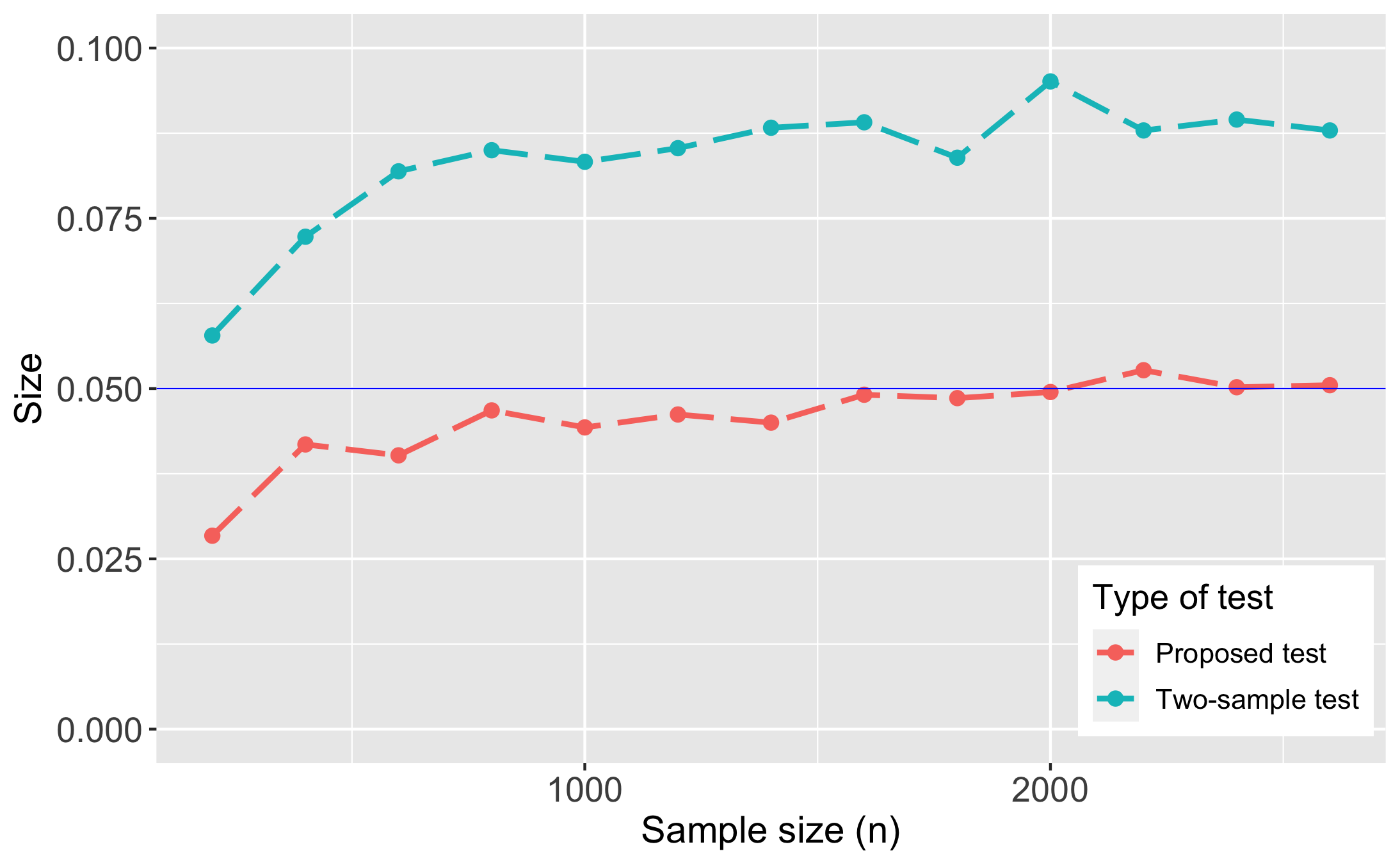
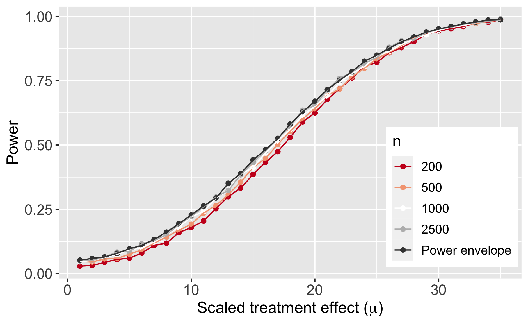
A: Size

B: Power function

Note: Panel A plots the size of $\hat{\varphi}$ along with that of the standard two-sample test at the nominal $5$% level (solid blue line) when the errors are drawn from a $\sqrt{3}\times\textrm{Uniform}[-1,1]$ distribution for each treatment. Panel B plots the finite sample power envelopes of $\hat{\varphi}$ under different $n$, along with asymptotic power envelope for unbiased tests. The scaled treatment effect is defined as $\mu=\sqrt{n}|\delta|$.

Figure 6.1. Finite sample performance of $\hat{\varphi}$ under horizontal boundary designs

6.2. Group sequential experiments

In this application, we suggest methods for inference on treatment effects following group sequential experiments. To simplify matters, suppose that the researchers assign the two treatments with equal probability in each stage. Let $\mu_{1},\mu_{0}$ denote the expectation of outcomes from the two treatments. Also, take $x_{n}(\cdot)$ to be the scaled difference in sample means, i.e., it is the quantity defined in (4.3) with $\psi_{1}(Y)=\psi_{0}(Y)=Y$. While there are a number of different group sequential designs, see, e.g., Wassmer and Brannath (2016) for a textbook overview, the general construction is that the experiment is terminated at the end of stage $t$ if $x_{n}(t)$ is outside some interval $\mathcal{I}_{t}$. The stopping time $\hat{\tau}$ thus satisfies $\{\hat{\tau}>t-1\}\equiv\cap_{l=1}^{t-1}\left\{x_{n}(l)\in\mathcal{I}_{l}\right\}$. The intervals $\{\mathcal{I}_{t}\}_{t=1}^{T}$ are pre-determined and chosen by balancing various ethical, cost and power criteria. We take them as given.

We are interested in testing the drifting hypotheses $H_{0}:\mu_{1}-\mu_{0}=\bar{\mu}/\sqrt{n}$ vs $H_{1}:\mu_{1}-\mu_{0}>\bar{\mu}/\sqrt{n}$ at some spending level $\bm{\alpha}$ that is chosen by experimenter. We can then invert these tests to obtain one-sided confidence intervals for the treatment effect $\mu_{1}-\mu_{0}$. The limit experiment in this setting consists of observing $x(t)\sim\sigma^{-1}\mu t+W(t)$, where $\mu:=\mu_{1}-\mu_{0}$, along with a discrete stopping time $\tau\in\{1,\dots,T\}$ such that $\{\tau>t-1\}$ if and only if $x(l)\in\mathcal{I}_{l}$ for all $l=1,\dots,t-1$. Let $\mathbb{P}_{\mu}(\cdot)$ denote the induced probability measure over the sample paths of $x(\cdot)$ between $0$ and $T$, and $\mathbb{E}_{\mu}[\cdot]$ its corresponding expectation. In view of the results in Section 2.4, the optimal level-$\bm{\alpha}$ test $\varphi^{*}(\cdot)$ of $H_{0}:\mu=\bar{\mu}$ vs $H_{1}:\mu>\bar{\mu}$ in the limit experiment is given by

$$\varphi^{*}(\tau,x(\tau))=\begin{cases}1&\textrm{if }\mathbb{P}_{\bar{\mu}}(\tau=t)\leq\alpha_{t}\\ \mathbb{I}\left\{x(t)\geq\gamma(t)\right\}&\textrm{if }\mathbb{P}_{\bar{\mu}}(\tau=t)>\alpha_{t},\end{cases}$$ (6.1)

where $\gamma(t)$ is chosen such that $\mathbb{E}_{\bar{\mu}}[\varphi^{*}(\tau,x(\tau))|\tau=t]=\alpha_{t}/\mathbb{P}_{\bar{\mu}}(\tau=t)$.

A finite sample version, $\hat{\varphi}$, of this test can be constructed by replacing $\tau,x(\tau)$ in $\varphi^{*}$ with $\hat{\tau},x_{n}(\hat{\tau})$. The resulting test would be asymptotically optimal under a suitable non-parametric version of the $\bm{\alpha}$-spending requirement. We refer to Appendix B.3 for the details and for the proof that $\hat{\varphi}$ is asymptotically optimal, in the sense that it attains the power of $\varphi^{*}$ in the limit experiment. A two-sided test for $H_{0}:\mu_{1}-\mu_{0}=\bar{\mu}/\sqrt{n}$ vs $H_{1}:\mu_{1}-\mu_{0}\neq\bar{\mu}/\sqrt{n}$ can be similarly constructed by imposing a conditional unbiasedness restriction as in Section 2.4.3.

6.2.1. Numerical Illustration

To illustrate the methodology, consider a group sequential trial based on the widely-used design of O’Brien and Fleming (1979), with $T=2$ stages. This corresponds to setting $\mathcal{I}_{1}=[-2.797,2.797]$. We would like to test $H_{0}:\mu_{1}-\mu_{0}=\bar{\mu}/\sqrt{n}$ vs $H_{1}:\mu_{1}-\mu_{0}>\bar{\mu}/\sqrt{n}$ at the spending level $(\alpha/\mathbb{P}_{\bar{\mu}}(\tau=1),\alpha/\mathbb{P}_{\bar{\mu}}(\tau=2))$, equivalent to a conditional size constraint, $\mathbb{P}_{\bar{\mu}}(\varphi=1|\tau=t)=\alpha\ \forall\ t$. Figure 6.2 Panel A plots the thresholds, $(\gamma(1),\gamma(2))$, for this test under $\alpha=0.05$ and $\sigma_{1}=\sigma_{0}=1$. Unsurprisingly, the thresholds are increasing in $\bar{\mu}$ , but it is interesting to observe that they cross at some $\bar{\mu}$.

To describe the finite sample performance of this test, we ran Monte-Carlo simulations with $Y_{i}^{(1)}=\bar{\mu}/\sqrt{n}+\epsilon_{i}^{(1)}$ and $Y_{i}^{(0)}=\epsilon_{i}^{(0)}$ where $\epsilon_{i}^{(1)},\epsilon_{i}^{(0)}\sim\sqrt{3}\times\textrm{Uniform}[-1,1]$. The treatments were sampled in equal proportions $(\pi=1/2$). Since $\sigma_{1},\sigma_{0}$ are unknown in practice, we estimate them using data from the first stage. Figure 6.2, Panel B plots the overall size of the test (which is the sum of the $\alpha$-spending values at each stage) for different values of $n$ and $\bar{\mu}$ under the nominal $\alpha$-spending level of $(0.05/\mathbb{P}_{\bar{\mu}}(\tau=1),0.05/\mathbb{P}_{\bar{\mu}}(\tau=2))$. We see that the asymptotic approximation worsens for larger values of $\bar{\mu}$, but overall, the size is close to nominal even for relatively small values of $n$.

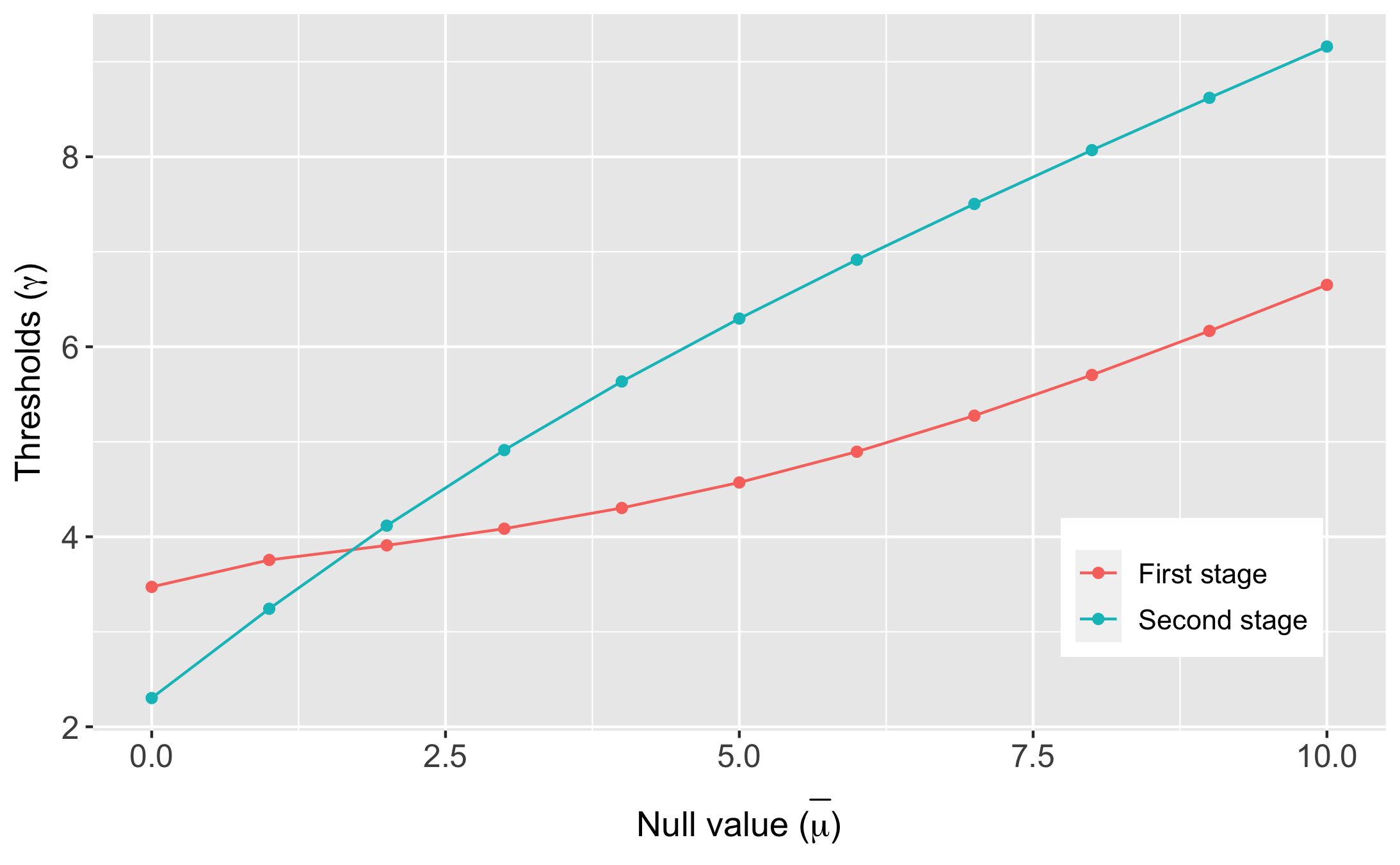
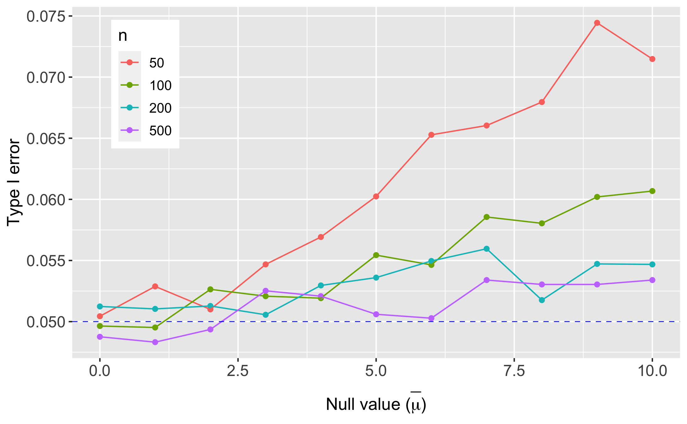
A: Critical values

B: Finite sample size

Note: Panel A plots the threshold values in each stage for the optimal, one-sided, level-$\bm{\alpha}$ test, (6.1), at the $(0.05/\mathbb{P}_{\bar{\mu}}(\tau=1),0.05/\mathbb{P}_{\bar{\mu}}(\tau=2))$ spending level. Panel B plots the overall type-I error in finite samples for different values of $n$ and null values, $\bar{\mu}$, when the errors are drawn from a $\sqrt{3}\times\textrm{Uniform}[-1,1]$ distribution for each treatment.

Figure 6.2. Testing in group sequential experiments

6.3. Bandit experiments

Here, we describe inferential procedures for the batched Thompson-sampling algorithm. For illustration, we employ $K=2$ treatments and $J=10$ batches. Let $(\bar{\mu}_{1},\bar{\mu}_{0})$ and $(\sigma_{1}^{2},\sigma_{0}^{2})$ denote the population means and variances for each treatment. For simplicity, we take $\sigma_{1}^{2}=\sigma_{0}^{2}=1$. The limit experiment can be described as follows: Suppose the decision maker (DM) employs the sampling rule $\pi_{j}^{(a)}$ in batch $j$. The DM then observes $Z_{j}^{(a)}\sim\mathcal{N}\left(\bar{\mu}_{a}\pi_{a},\pi_{a}\right)$ for $a\in\{0,1\}$ and updates the state variables $x_{a},q_{a}$ (which are initially set to $0$) as

$$x_{a}\leftarrow x_{a}+Z_{j}^{(a)},\quad q_{a}\leftarrow q_{a}+\pi_{a}.$$

Under an under-smoothed prior, suggested by Wager and Xu (2021), the Thompson sampling rule in batch $j+1$ is

$$\pi_{j+1}^{(1)}=\Phi\left(\frac{q_{1}^{-1}x_{1}-q_{0}^{-1}x_{0}}{\sqrt{j/q_{1}q_{0}}}\right).$$

We set $\pi_{1}^{(a)}=1/2$ for first batch. In what follows, we let $\mu_{a}:=J\bar{\mu}_{a}$. We are interested in testing $H_{0}:(\mu_{1},\mu_{0})=(0,0)$.

Figure 6.3, Panel A plots the asymptotic power envelope for testing $H_{0}:(\mu_{1},\mu_{2})=(0,0)$. Clearly, the envelope is not symmetric; distinguishing $(a,0)$ from $(0,0)$ is easier than distinguishing $(-a,0)$ from $(0,0)$ for any $a>0$. This is because of the asymmetry in treatment allocation under Thompson sampling; under $(-a,0)$, treatment 1 is sampled more often than treatment $0$ but the data from treatment $1$ is uninformative for distinguishing $(-a,0)$ from $(0,0)$.

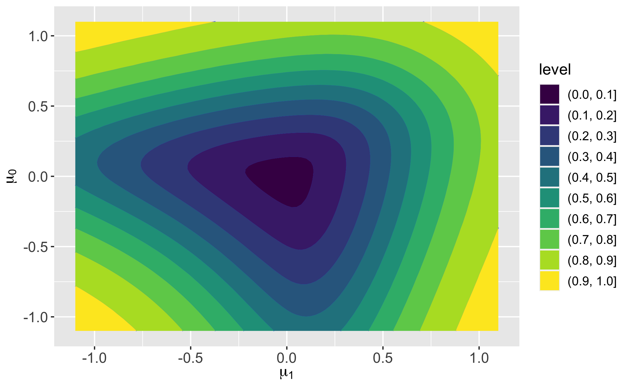
Note: The figure plots the asymptotic power envelope for any test of $H_{0}:(\mu,\mu)=(0,0)$ against different values $(\mu_{1},\mu_{0})$ under the alternative.

Figure 6.3. Power envelope for Thompson-sampling with $10$ batches

6.3.1. Numerical illustration

To determine the accuracy of our asymptotic approximations, we ran Monte-Carlo simulations with $Y_{i}^{(a)}=\mu_{a}+\epsilon_{i}^{(a)}$ where $\epsilon_{i}^{(1)},\epsilon_{i}^{(0)}\sim\sqrt{3}\times\textrm{Uniform}[-1,1]$. Figure 6.4, Panel A plots the finite sample performance of the Neyman-Pearson tests in the limit experiment for testing $H_{0}:(\mu_{1},\mu_{0})=(0,0)$ vs $H_{1}:(\mu_{1},\mu_{0})=(\mu,\mu)$ under various values of $\mu$ (due to symmetry, we only report the results for positive $\mu$). Panel B repeats the same calculation, but against alternatives of the form $H_{1}:(\mu,0)$. As noted earlier, power is higher here for $\mu>0$ as opposed to $\mu<0$. Both plots show that the asymptotic approximation is quite accurate even for $n$ as small as $20$ (note that the number of batches is $10$, so this corresponds to $200$ observations overall). The approximation is somewhat worse for testing $\mu<0$; this is because Thompson-sampling allocates much fewer units to treatment 0 in this instance, even though it is only data from this treatment that is informative for distinguishing the two hypotheses.

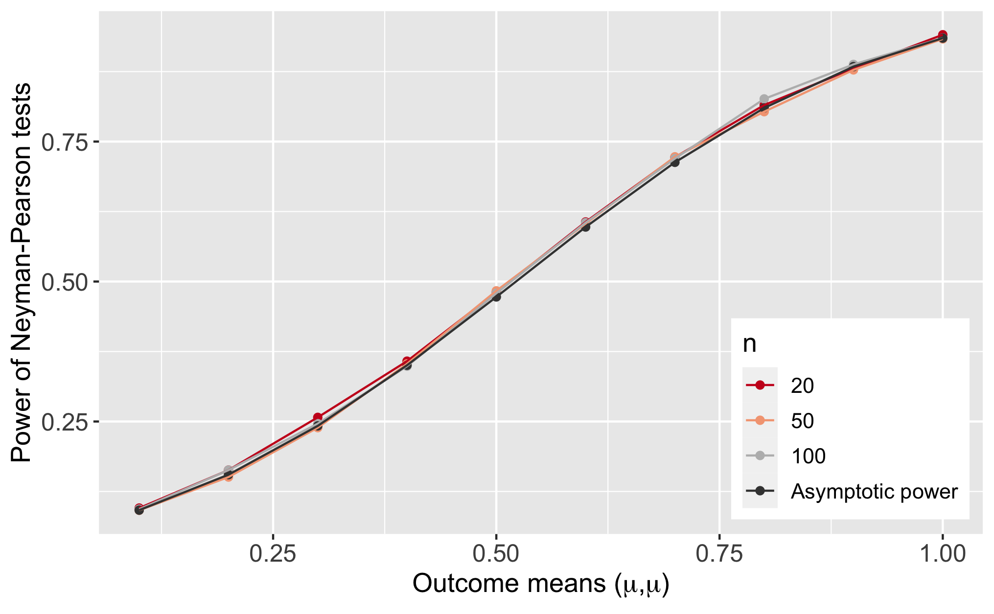
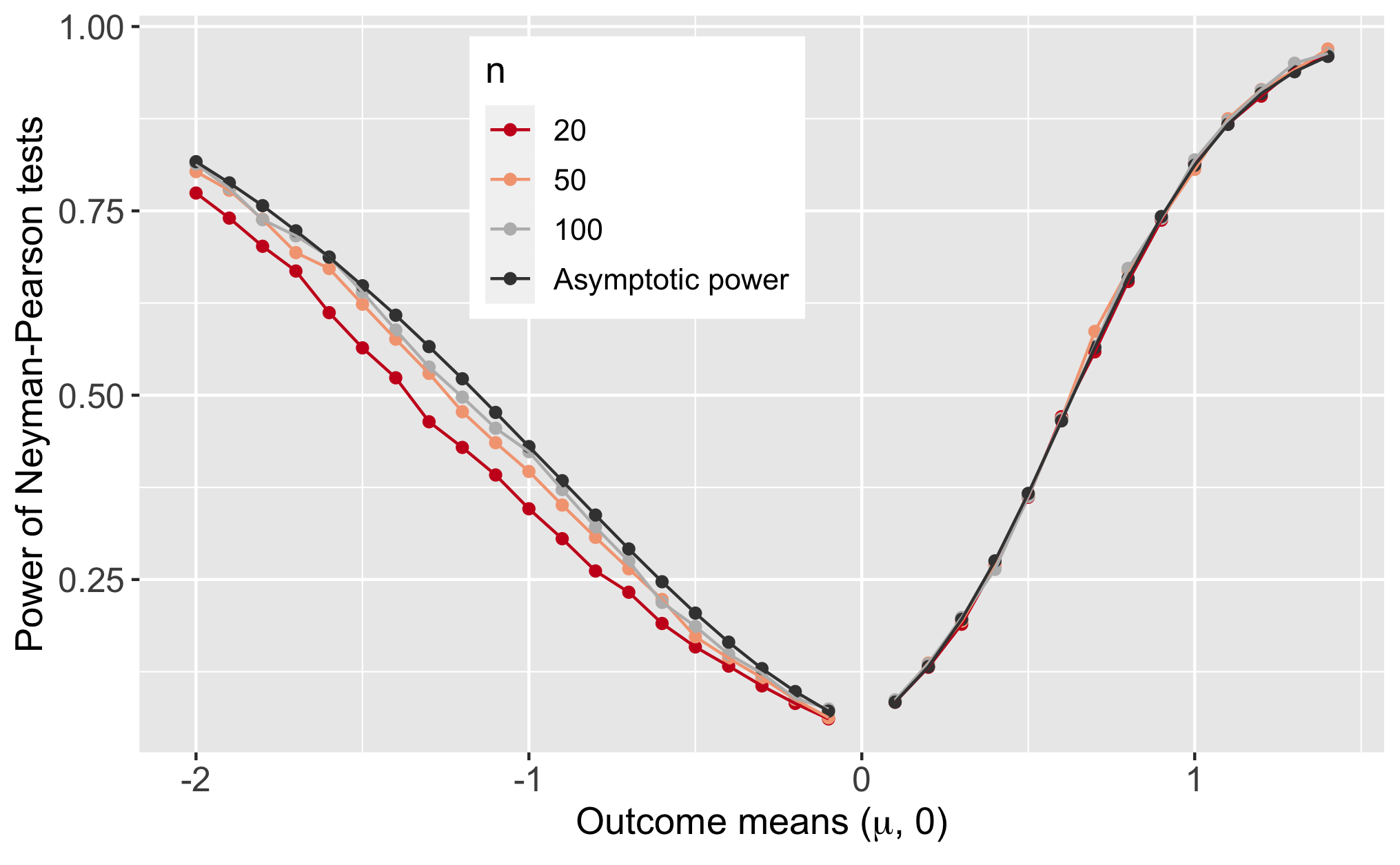
A: Power against $H_{1}:(\mu,\mu)$

B: Power against $H_{1}:(\mu,0)$

Note: Panel A plots the finite sample power of Neyman-Pearson tests at the nominal $5$% level (solid blue line) for testing $H_{0}:(\mu_{1},\mu_{0})=(0,0)$ against $H_{1}:(\mu_{1},\mu_{0})=(\mu,\mu)$ when the errors are drawn from a $\sqrt{3}\times\textrm{Uniform}[-1,1]$ distribution for each treatment. Panel B repeats the same calculation for alternatives of the form $H_{1}:(\mu_{1},\mu_{0})=(\mu,0)$. Both panels also display the asymptotic power envelope.

Figure 6.4. Finite sample performance of Neyman-Pearson tests in bandit experiments

7. Conclusion

Conducting inference after sequential experiments is a challenging task. However, significant progress can be made by analyzing the optimal inference problem under an appropriate limit experiment. We showed that the data from any sequential experiment can be condensed into a finite number of sufficient statistics, while still maintaining the power of tests. Furthermore, we were able to establish uniquely optimal tests under reasonable constraints such as unbiasedness and $\bm{\alpha}$-spending, in both parametric and non-parametric regimes. Taken together, these findings offer a comprehensive framework for conducting optimal inference following sequential experiments.

Despite these results, there are still several avenues for future research. While we believe that our results for experiments with adaptive sampling rules apply without batching, this needs be formally verified. Our characterization of uniquely optimal tests is also limited in this context, as $\bm{\alpha}$-spending restrictions are not feasible. Therefore, exploring other types of testing considerations such as invariance or conditional inference may be worthwhile. We believe that the techniques developed in this paper will prove useful for analyzing these other types of tests.

Appendix A Proofs

A.1. Proof of Theorem 1

To prove the first claim, observe that both $\hat{\tau}$ and $x_{n}(\hat{\tau})$ are tight under $P_{nT,0}$: the former by Assumption 2, and the latter by the fact $\max_{t\leq T}x_{n}(t)$ is tight (by the continuous mapping theorem it converges to the tight limit $\max_{t}x(t)$ under $P_{nT,0}$). Hence, the joint $(\hat{\tau},x_{n}(\hat{\tau}))$ is a also tight, and by Prohorov’s theorem, converges in distribution under sub-sequences. The first part of the theorem then follows from Le Cam (1979, Theorem 1).

To prove the second claim, denote ${\bf y}_{nt}=(Y_{1},\dots,Y_{nt})$. Defining

$$\ln\frac{dP_{nt,h}}{dP_{nt,0}}({\bf y}_{nt})=\sum_{i=1}^{\left\lfloor nt\right\rfloor}\ln\frac{dp_{\theta_{0}+h/\sqrt{n}}}{dp_{\theta_{0}}}(Y_{i}),$$

we have by the SLAN property, (2.3), and Assumption 1(i) that

$$\ln\frac{dP_{n\hat{\tau},h}}{dP_{n\hat{\tau},0}}({\bf y}_{n\hat{\tau}})=h^{\intercal}I^{1/2}x_{n}(\hat{\tau})-\frac{\hat{\tau}}{2}h^{\intercal}Ih+o_{P_{nT,0}}(1).$$

Combining the above with the first part of the theorem gives

$$\ln\frac{dP_{n\hat{\tau},h}}{dP_{n\hat{\tau},0}}({\bf y}_{n\hat{\tau}})\xrightarrow[P_{nT,0}]{d}h^{\intercal}I^{1/2}x(\tau)-\frac{\tau}{2}h^{\intercal}Ih,$$ (A.1)

where $x(\cdot)$ has the same distribution as $d$-dimensional Brownian motion.

Now, $\varphi_{n}$ is tight since $\varphi_{n}\in[0,1]$. Together with (A.1), this implies the joint $\left(\varphi_{n},\ln\frac{dP_{n\hat{\tau},h}}{dP_{n\hat{\tau},0}}({\bf y}_{n\hat{\tau}})\right)$ is also tight. Hence, by Prohorov’s theorem, given any sequence $\{n_{j}\}$, there exists a further sub-sequence $\{n_{j_{m}}\}$ - represented as $\{n\}$ without loss of generality - such that

$$\left(\begin{array}[]{c}\varphi_{n}\\ \frac{dP_{n\hat{\tau}.,h}}{dP_{n\hat{\tau},0}}\left({\bf y}_{n\hat{\tau}}\right)\end{array}\right)\xrightarrow[P_{nT,0}]{d}\left(\begin{array}[]{c}\bar{\varphi}\\ V\end{array}\right);\quad V\sim\exp\left\{h^{\intercal}I^{1/2}x(\tau)-\frac{\tau}{2}h^{\intercal}Ih\right\},$$ (A.2)

where $\bar{\varphi}\in[0,1]$. It is a well known property of Brownian motion that $M(t):=\exp\left\{h^{\intercal}I^{1/2}x(t)-\frac{t}{2}h^{\intercal}Ih\right\}$ is a martingale with respect to the filtration $\mathcal{F}_{t}$. Since $\tau$ is an $\mathcal{F}_{t}$-adapted stopping time, the optional stopping theorem then implies $E[V]\equiv E[M(\tau)]=E[M(0)]=1$.

We now claim that

$$\varphi_{n}\xrightarrow[P_{nT,h}]{d}L;\ \textrm{where }L(B):=E[\mathbb{I}\{\bar{\varphi}\in B\}V]\ \forall\ B\in\mathcal{B}(\mathbb{R}).$$ (A.3)

It is clear from $V\geq 0$ and $E[V]=1$ that $L(\cdot)$ is a probability measure, and that for every measurable function $f:\mathbb{R}\to\mathbb{R}$, $\int fdL=E[f(\bar{\varphi})V]$. Furthermore, for any $f(\cdot)$ lower-semicontinuous and non-negative,

$$\lim\inf\mathbb{E}_{nT,h}[f(\varphi_{n})] \geq\lim\inf\mathbb{E}_{nT,0}\left[f(\varphi_{n})\frac{dP_{nT,h}}{dP_{nT,0}}\right]$$

$$=\lim\inf\mathbb{E}_{nT,0}\left[f(\varphi_{n})\frac{dP_{n\hat{\tau},h}}{dP_{n\hat{\tau},0}}\right]\geq E[f(\bar{\varphi})V],$$

where the equality follows from the law of iterated expectations since $\varphi_{n}$ is a function only of ${\bf y}_{n\hat{\tau}}$ and $dP_{n\hat{\tau},h}/dP_{n\hat{\tau},0}$ is a martingale under $P_{nT,0}$; and the last inequality follows from applying the portmanteau lemma on (A.2). Finally, applying the portmanteau lemma again, in the converse direction, gives (A.3).

Since $\varphi_{n}$ is bounded, (A.3) implies

$$\lim_{n\to\infty}\beta_{n}(h):=\lim_{n\to\infty}\mathbb{E}_{nT,h}\left[\varphi_{n}\right]=E\left[\bar{\varphi}e^{h^{\intercal}I^{1/2}x(\tau)-\frac{\tau}{2}h^{\intercal}Ih}\right].$$ (A.4)

Define $\varphi(\tau,x(\tau)):=E[\bar{\varphi}|\tau,x(\tau)]$; this is a test statistic since $\varphi\in[0,1]$. The right hand side of (A.4) then becomes

$$E\left[\varphi(\tau,x(\tau))e^{h^{\intercal}I^{1/2}x(\tau)-\frac{\tau}{2}h^{\intercal}Ih}\right].$$

But by the Girsanov theorem, this is just the expectation, $\mathbb{E}_{h}[\varphi(\tau,x(\tau))]$, of $\varphi(\tau,x(\tau))$ when $x(t)$ is distributed as a Gaussian process with drift $I^{1/2}h$, i.e., when $x(t)\sim I^{1/2}ht+W(t)$.

A.2. Proof of Proposition 1

We start by proving the first claim. Denote $H_{0}\equiv\{h:a^{\intercal}h=0\}$ and $H_{1}\equiv\{h:a^{\intercal}h=c\}$. Let $\mathbb{P}_{h}$ denote the induced probability measure over the sample paths generated by $x(t)\sim I^{1/2}ht+W(t)$ between $t\in[0,T]$. As before, $\mathcal{F}_{t}$ denotes the filtration generated by $\{U,x(s):s\leq t\}$. Given any $h_{1}\in H_{1}$, define $h_{0}=h_{1}-(a^{\intercal}h_{1}/a^{\intercal}I^{-1}a)I^{-1}a$. Note that $a^{\intercal}h_{1}=c$ and $h_{0}\in H_{0}$. Let $\ln\frac{d\mathbb{P}_{h_{1}}}{d\mathbb{P}_{h_{0}}}(\mathcal{F}_{t})$ denote the likelihood ratio between the probabilities induced by the parameters $h_{1},h_{0}$ over the filtration $\mathcal{F}_{t}$. By the Girsanov theorem,

$$\ln\frac{d\mathbb{P}_{h_{1}}}{d\mathbb{P}_{h_{0}}}(\mathcal{F}_{\tau}) =\left(h_{1}^{\intercal}I^{1/2}x(\tau)-\frac{\tau}{2}h_{1}^{\intercal}Ih_{1}\right)-\left(h_{0}^{\intercal}I^{1/2}x(\tau)-\frac{\tau}{2}h_{0}^{\intercal}Ih_{0}\right)$$

$$=\frac{1}{\sigma}c\tilde{x}(\tau)-\frac{c^{2}}{2\sigma^{2}}\tau,$$

where $\tilde{x}(t):=\sigma^{-1}a^{\intercal}I^{-1/2}x(t)$. Hence, an application of the Neyman-Pearson lemma shows that the UMP test of $H_{0}^{\prime}:h=h_{0}$ vs $H_{1}^{\prime}:h=h_{1}$ is given by

$$\varphi_{c}^{*}=\mathbb{I}\left\{c\tilde{x}(\tau)-\frac{c^{2}}{2\sigma}\tau\geq\gamma\right\},$$

where $\gamma$ is chosen by the size requirement. Now, for any $h_{0}\in H_{0}$,

$$\tilde{x}(t)\equiv\sigma^{-1}a^{\intercal}I^{-1/2}x(t)\sim W(t).$$

Hence, the distribution of the sample paths of $\tilde{x}(\cdot)$ is independent of $h_{0}$ under the null. Combined with the assumption that $\tau$ is $\tilde{\mathcal{F}}_{t}$-adapted, this implies $\varphi_{c}^{*}$ does not depend on $h_{0}$ and, by extension, $h_{1}$, except through $c$. Since $h_{1}\in H_{1}$ was arbitrary, we are led to conclude $\varphi_{c}^{*}$ is UMP more generally for testing $H_{0}:a^{\intercal}h=0$ vs $H_{1}:a^{\intercal}h=c$.

The second claim is an easy consequence of the first claim and Theorem 1.

A.3. Proof of Proposition 2

By the Girsanov theorem,

$$\beta(h):=\mathbb{E}_{h}[\varphi]=\mathbb{E}_{0}\left[\varphi(\tau,x(\tau))e^{h^{\intercal}I^{1/2}x(\tau)-\frac{\tau}{2}h^{\intercal}Ih}\right].$$

It can be verified from the above that $\beta(h)$ is differentiable around $h=0$. But unbiasedness requires $\mathbb{E}_{h}[\varphi]\geq\alpha$ for all $h$ and $\mathbb{E}_{0}[\varphi]=\alpha$. This is only possible if $\beta^{\prime}(0)=0$, i.e., $\mathbb{E}_{0}[x(\tau)\varphi(\tau,x(\tau))]=0$.

A.4. Proof of Theorem 2

Since $\hat{\tau}$ is bounded, it follows by similar arguments as in the proof of Theorem 1 that $\left(\varphi_{n},\hat{\tau},\ln\frac{dP_{n\hat{\tau},h}}{dP_{n\hat{\tau},0}}({\bf y}_{n\hat{\tau}})\right)$ is tight. Consequently, by Prohorov’s theorem, given any sequence $\{n_{j}\}$, there exists a further sub-sequence $\{n_{j_{m}}\}$ - represented as $\{n\}$ without loss of generality - such that

$$\left(\begin{array}[]{c}\varphi_{n}\\ \hat{\tau}\\ \frac{dP_{n\hat{\tau}.,h}}{dP_{n\hat{\tau},0}}\left({\bf y}_{n\hat{\tau}}\right)\end{array}\right)\xrightarrow[P_{nT,0}]{d}\left(\begin{array}[]{c}\bar{\varphi}\\ \tau\\ V\end{array}\right);\quad V\sim\exp\left\{h^{\intercal}I^{1/2}x(\tau)-\frac{\tau}{2}h^{\intercal}Ih\right\}.$$ (A.5)

It then follows as in the proof of Theorem 1 that

$$\left(\begin{array}[]{c}\varphi_{n}\\ \hat{\tau}\end{array}\right)\xrightarrow[P_{nT,h}]{d}L;\ \textrm{where }L(B):=E[\mathbb{I}\{(\bar{\varphi},\tau)\in B\}V]\ \forall\ B\in\mathcal{B}(\mathbb{R}^{2}).$$ (A.6)

The above in turn implies

$$\lim_{n\to\infty}\mathbb{E}_{nT,h}\left[\varphi_{n}\mathbb{I}\{\hat{\tau}=t\}\right] =E\left[\bar{\varphi}\mathbb{I}\{\tau=t\}e^{h^{\intercal}I^{1/2}x(\tau)-\frac{\tau}{2}h^{\intercal}Ih}\right],\ \textrm{and }$$ (A.7)

$$\lim_{n\to\infty}\mathbb{E}_{nT,h}\left[\mathbb{I}\{\hat{\tau}=t\}\right] =E\left[\mathbb{I}\{\tau=t\}e^{h^{\intercal}I^{1/2}x(\tau)-\frac{\tau}{2}h^{\intercal}Ih}\right].$$ (A.8)

for every $t\in\{1,2,\dots,T\}$.

Denote $\varphi(\tau,x(\tau))=E[\bar{\varphi}|\tau,x(\tau)]$; this is a level-$\bm{\alpha}$ test, as can be verified by setting $h=0$ in (A.7). The right hand side of (A.7) then becomes

$$E\left[\varphi(\tau,x(\tau))\mathbb{I}\{\tau=t\}e^{h^{\intercal}I^{1/2}x(\tau)-\frac{\tau}{2}h^{\intercal}Ih}\right].$$

An application of the Girsanov theorem then shows that the right hand sides of (A.7) and (A.8) are just the expectations, $\mathbb{E}_{h}[\varphi(\tau,x(\tau))\mathbb{I}\{\tau=t\}]$ and $\mathbb{E}_{h}[\mathbb{I}\{\tau=t\}]$ when $x(t)\sim I^{1/2}ht+W(t)$. What is more, the measures $\mathbb{P}_{0}(\cdot),\mathbb{P}_{h}(\cdot)$ are absolutely continuous, so $\mathbb{P}_{0}(\tau=t)=0$ if and only if $\mathbb{P}_{h}(\tau=t)=0$ for any $h\in\mathbb{R}^{d}$. We are thus led to conclude that

$$\lim_{n\to\infty}\beta_{n}(h|t):=\lim_{n\to\infty}\frac{\mathbb{E}_{nT,h}\left[\varphi_{n}\mathbb{I}\{\hat{\tau}=t\}\right]}{\mathbb{E}_{nT,h}\left[\mathbb{I}\{\hat{\tau}=t\}\right]}=\frac{\mathbb{E}_{h}\left[\varphi_{n}\mathbb{I}\{\hat{\tau}=t\}\right]}{\mathbb{E}_{h}\left[\mathbb{I}\{\hat{\tau}=t\}\right]}:=\beta(h|t)$$

for every $h\in\mathbb{R}^{d}$, and $t\in\{1,2,\dots,T\}$ satisfying $\mathbb{P}_{0}(\tau=t)\neq 0$. This proves the desired claim.

A.5. Proof of Proposition 3

Fix some arbitrary $g_{1}\in T(P_{0})$. To simplify matters, we set $\delta=1$. The case of general $\delta$ can be handled by simply replacing $g_{1}$ with $g_{1}/\delta$. By standard results for Hilbert spaces, we can write $g_{1}=\sigma^{-1}\left\langle\psi,g\right\rangle(\psi/\sigma)+\tilde{g}_{1}$, where $\tilde{g}_{1}\perp(\psi/\sigma)$ . Define $\bm{g}:=\left(\psi/\sigma,\tilde{g}_{1}/\left\|\tilde{g}_{1}\right\|\right)^{\intercal}$, and consider sub-models of the form $P_{1/\sqrt{n},\bm{h}^{\intercal}\bm{g}}$ for $\bm{h}\in\mathbb{R}^{2}$. By (3.2),

$$\sum_{i=1}^{\left\lfloor nt\right\rfloor}\ln\frac{dP_{1/\sqrt{n},\bm{h}^{\intercal}\bm{g}}}{dP_{0}}(Y_{i})=\frac{\bm{h}^{\intercal}}{\sqrt{n}}\sum_{i=1}^{\left\lfloor nt\right\rfloor}\bm{g}(Y_{i})-\frac{t}{2}\bm{h}^{\intercal}\bm{h}+o_{P_{nT,0}}(1),\ \textrm{ uniformly over }t.$$ (A.9)

Comparing with (2.3), we observe that $\left\{P_{1/\sqrt{n},\bm{h}^{\intercal}\bm{g}}:\bm{h}\in\mathbb{R}^{2}\right\}$ is equivalent to a parametric model with score $\bm{g}(\cdot)$ and local parameter $\bm{h}$ (note that $\mathbb{E}_{P_{0}}[\bm{g}\bm{g}^{\intercal}]=I$). Let $G_{n}(t):=n^{-1/2}\sum_{i=1}^{n}\bm{g}(Y_{i})$ denote the score process. By the functional central limit theorem, $G_{n}(t)\xrightarrow[P_{nT,0}]{d}G(t)\equiv(x(t),\tilde{G}(t))$, where $x(\cdot),\tilde{G}(\cdot)$ are independent one-dimensional Brownian motions. Take $\mathcal{G}_{t}:=\sigma\{G(s):s\leq t\}$, $\mathcal{F}_{t}:=\sigma\{x(s):s\leq t\}$ to be the filtrations generated by $G(\cdot)$ and $x(\cdot)$ respectively until time $t$. Since the first component of $G_{n}(\cdot)$ is $x_{n}(\cdot)$ and $\hat{\tau}=\tau(x_{n}(\cdot))$ by Assumption 3(ii), the extended continuous mapping theorem implies

$$(G_{n}(\hat{\tau}),\hat{\tau})\xrightarrow[P_{nT,0}]{d}(G(\tau),\tau),$$ (A.10)

where $\tau$ is a $\mathcal{F}_{t}$-adapted stopping time, and therefore, $\mathcal{G}_{t}$-adapted by extension.

Consider the limit experiment where one observes a $\mathcal{F}_{t}$-adapted stopping time $\tau$ along with a diffusion process $G(t):=\bm{h}t+W(t)$, where $W(\cdot)$ is 2-dimensional Brownian motion. Using (A.9) and (A.10), we can argue as in the proof of Theorem 1 to show that any test in the parametric model $\left\{P_{1/\sqrt{n},\bm{h}^{\intercal}\bm{g}}:\bm{h}\in\mathbb{R}^{2}\right\}$ can be matched (along sub-sequences) by a test that depends only on $G(\tau),\tau$ in the limit experiment. Hence, $\beta_{n}\left(\bm{h}^{\intercal}\bm{g}\right):=\int\varphi_{n}dP_{nT,\bm{h}^{\intercal}\bm{g}}$ converges along sub-sequences to the power function, $\beta(\bm{h})$, of some test $\varphi(\tau,G(\tau))$ in the limit experiment. Note that by our definitions, $\left\langle\psi,\bm{h}^{\intercal}\bm{g}\right\rangle$ is simply the first component of $\bm{h}$ divided by $\sigma$. This in turn implies, as a consequence of the definition of asymptotically level-$\alpha$ tests, that $\varphi(\cdot)$ is level-$\alpha$ for testing $H_{0}:(1,0)^{\intercal}\bm{h}=0$ in the limit experiment.

Now, by a similar argument as in the proof of Proposition 1, along with the fact $(1,0)^{\intercal}G(t)=x(t)$, the optimal level-$\alpha$ test of $H_{0}:(1,0)^{\intercal}\bm{h}=0$ vs $H_{1}:(1,0)^{\intercal}\bm{h}=\mu_{1}/\sigma$ in the limit experiment is given by

$$\varphi_{\mu_{1}}^{*}(\tau,x(\tau)):=\mathbb{I}\left\{\mu_{1}x(\tau)-\frac{\mu_{1}^{2}}{2\sigma}\tau\geq\gamma\right\}.$$

For all $\bm{h}\in H_{1}\equiv\{\bm{h}:(1,0)^{\intercal}\bm{h}=\mu_{1}/\sigma\}$ satisfying the alternative hypothesis,

$$x(t)=(1,0)^{\intercal}G(t)\sim\sigma^{-1}\mu_{1}t+\tilde{W}(t),$$

where $\tilde{W}(\cdot)$ is 1-dimensional Brownian motion. As $\tau$ is $\mathcal{F}_{t}$-adapted, the joint distribution of $(\tau,x(\tau))$ therefore depends only on $\mu_{1}$ for $\bm{h}\in H_{1}$. Consequently, the power, $\mathbb{E}_{\bm{h}}[\varphi_{\mu_{1}}^{*}(\tau,x(\tau))]$, of $\varphi_{\mu_{1}}^{*}(\cdot)$ against such alternatives depends only on $\mu_{1}$, and is denoted by $\beta^{*}\left(\mu_{1}\right)$. Since $\varphi_{\mu_{1}}^{*}(\cdot)$ is the optimal test and $\mu_{1}=\left\langle\psi,\bm{h}^{\intercal}\bm{g}\right\rangle$, we conclude $\beta(\bm{h})\leq\beta^{*}\left(\left\langle\psi,\bm{h}^{\intercal}\bm{g}\right\rangle\right)$. This further implies $\lim\sup_{n}\beta_{n}(\bm{h}^{\intercal}\bm{g})\leq\beta^{*}\left(\left\langle\psi,\bm{h}^{\intercal}\bm{g}\right\rangle\right)$ for any $\bm{h}\in\mathbb{R}^{2}$. Setting $\bm{h}=\left(\left\langle\psi,g_{1}\right\rangle/\sigma,\left\|\tilde{g}_{1}\right\|\right)^{\intercal}$ then gives $\lim\sup_{n}\beta_{n}(g_{1})\leq\beta^{*}\left(\left\langle\psi,g_{1}\right\rangle\right)$. Since $g_{1}\in T(P_{0})$ was arbitrary, the claim follows.

A.6. Proof of Proposition 5

For some arbitrary $\bm{g}=(g_{1},g_{0})\in T(P_{0}^{(1)})\times T(P_{0}^{(0)})$. To simplify matters, we set $\delta_{1}=\delta_{0}=1$. The case of general $\delta$ can be handled by simply replacing $g_{a}$ with $g_{a}/\delta_{a}$. In what follows, let $\pi_{1}=\pi$ and $\pi_{0}=1-\pi$. The vectors ${\bf y}_{nt}^{(1)}=(Y_{1}^{(1)},\dots,Y_{n\pi_{1}t}^{(1)})$ and ${\bf y}_{nt}^{(0)}=(Y_{1}^{(0)},\dots,Y_{n\pi_{0}t}^{(0)})$ denote the collection of outcomes from treatments 1 and 0 until time $t$, and we set ${\bf y}_{nt}=({\bf y}_{nt}^{(1)},{\bf y}_{nt}^{(0)})$. Define $P_{nt,\bm{g}}$ as the joint probability measure over ${\bf y}_{nt}$ when each $Y_{i}^{(a)}$ is an iid draw from $P_{1/\sqrt{n},g_{a}}^{(a)}$.

As in the proof of Proposition 3, we can write $g_{a}=\sigma_{a}^{-1}\left\langle\psi_{a},g_{a}\right\rangle_{a}(\psi_{a}/\sigma_{a})+\tilde{g}_{a}$, where $\tilde{g}_{a}\perp(\psi_{a}/\sigma_{a})$. Define $\bm{g}_{a}:=\left(\psi_{a}/\sigma_{a},\tilde{g}_{a}/\left\|\tilde{g}_{a}\right\|_{a}\right)^{\intercal}$, and consider sub-models of the form $P_{1/\sqrt{n},\bm{h}_{1}^{\intercal}\bm{g}_{1}}\times P_{1/\sqrt{n},\bm{h}_{0}^{\intercal}\bm{g}_{0}}$ for $\bm{h}_{1},\bm{h}_{0}\in\mathbb{R}^{2}$. By the SLAN property, (3.2), and the fact that the treatments are independent,

$$\ln\frac{dP_{nt,(\text{$\bm{h}_{1}^{\intercal}\bm{g}_{1}$},\bm{h}_{0}^{\intercal}\bm{g}_{0})}}{dP_{nt,\bm{0}}}({\bf y}_{nt})=\frac{\bm{h}_{1}^{\intercal}}{\sqrt{n}}\sum_{i=1}^{\left\lfloor n\pi_{1}t\right\rfloor}\bm{g}_{1}(Y_{i}^{(1)})-\frac{\pi_{1}t}{2}\bm{h}_{1}^{\intercal}\bm{h}_{1}+\dots$$

$$\qquad\dots+\frac{\bm{h}_{0}^{\intercal}}{\sqrt{n}}\sum_{i=1}^{\left\lfloor n\pi_{0}t\right\rfloor}\bm{g}_{0}(Y_{i}^{(0)})-\frac{\pi_{0}t}{2}\bm{h}_{0}^{\intercal}\bm{h}_{0}+o_{P_{nT,0}}(1),\ \textrm{ uniformly over }t.$$ (A.11)

Let $G_{a,n}(t):=n^{-1/2}\sum_{i=1}^{\left\lfloor n\pi_{a}t\right\rfloor}\bm{g}_{a}(Y_{i}^{(a)})$ for $a\in\{0,1\}$. By a standard functional central limit theorem,

$$G_{a,n}(t)\xrightarrow[P_{nT,\bm{0}}]{d}G_{a}(t)\equiv(z_{a}(t),\tilde{G}_{a}(t)),$$

where $z_{a}(\cdot)/\sqrt{\pi_{a}},\tilde{G}_{a}(\cdot)/\sqrt{\pi_{a}}$ are independent 1-dimensional Brownian motions. Furthermore, since the treatments are independent of each other, $G_{1}(\cdot),G_{0}(\cdot)$ are independent Gaussian processes. Define $\sigma^{2}:=\left(\frac{\sigma_{1}^{2}}{\pi_{1}}+\frac{\sigma_{0}^{2}}{\pi_{0}}\right)$,

$$x(t):=\frac{1}{\sigma}\left(\frac{\sigma_{1}}{\pi_{1}}z_{1}(t)-\frac{\sigma_{0}}{\pi_{0}}z_{0}(t)\right)$$

and take $\mathcal{G}_{t}:=\sigma\{(G_{1}(s),G_{0}(s)):s\leq t\}$, $\mathcal{F}_{t}:=\sigma\{x(s):s\leq t\}$ to be the filtrations generated by $\bm{G}(\cdot):=(G_{1}(\cdot),G_{0}(\cdot))$ and $x(\cdot)$ respectively until time $t$. Using Assumption 3(ii), the extended continuous mapping theorem implies

$$(G_{1,n}(\hat{\tau}),G_{0,n}(\hat{\tau}),\hat{\tau})\xrightarrow[P_{nT,0}]{d}(G_{1}(\tau),G_{0}(\tau),\tau),$$ (A.12)

where $\tau$ is a $\mathcal{F}_{t}$-adapted stopping time, and thereby $\mathcal{G}_{t}$-adapted, by extension.

Consider the limit experiment where one observes a $\mathcal{G}_{t}$-adapted stopping time $\tau$ along with diffusion processes $G_{a}(t):=\pi_{a}\bm{h}_{a}t+\sqrt{\pi_{a}}W_{a}(t),\ a\in\{0,1\}$, where $W_{1}(\cdot),W_{0}(\cdot)$ are independent 2-dimensional Brownian motions. By Lemma 2 in Appendix B, any test in the parametric model $\left\{P_{1/\sqrt{n},\bm{h}_{1}^{\intercal}\bm{g}_{1}}\times P_{1/\sqrt{n},\bm{h}_{0}^{\intercal}\bm{g}_{0}}:\bm{h}_{1},\bm{h}_{0}\in\mathbb{R}^{2}\right\}$ can be matched (along sub-sequences) by a test that depends only on $\bm{G}(\tau),\tau$ in the limit experiment. Hence,

$$\beta_{n}(\text{$\bm{h}_{1}^{\intercal}\bm{g}_{1}$},\bm{h}_{0}^{\intercal}\bm{g}_{0}):=\int\varphi_{n}dP_{nT,(\text{$\bm{h}_{1}^{\intercal}\bm{g}_{1}$},\bm{h}_{0}^{\intercal}\bm{g}_{0})}$$

converges along sub-sequences to the power function, $\beta(\bm{h}_{1},\bm{h}_{0})$, of some test $\varphi(\tau,\bm{G}(\tau))$ in the limit experiment. Note that by our definitions, the first component of $\bm{h}_{a}$ is $\left\langle\psi_{a},\bm{h}_{a}^{\intercal}\bm{g}_{a}\right\rangle_{a}/\sigma_{a}$. This in turn implies, as a consequence of the definition of asymptotically level-$\alpha$ tests, that $\varphi(\cdot)$ is level-$\alpha$ for testing $H_{0}:(\sigma_{1},0)^{\intercal}\bm{h}_{1}-(\sigma_{0},0)^{\intercal}\bm{h}_{0}=0$ in the limit experiment.

Now, by Lemma 3 in Appendix B, the optimal level-$\alpha$ test of $H_{0}:(\sigma_{1},0)^{\intercal}\bm{h}_{1}-(\sigma_{0},0)^{\intercal}\bm{h}_{0}=0$ vs $H_{1}:(\sigma_{1},0)^{\intercal}\bm{h}_{1}-(\sigma_{0},0)^{\intercal}\bm{h}_{0}=\mu$ in the limit experiment is

$$\varphi_{\mu}^{*}(\tau,x(\tau)):=\mathbb{I}\left\{\mu x(\tau)-\frac{\mu^{2}}{2\sigma}\tau\geq\gamma\right\}.$$

For all $\bm{h}\in H_{1}\equiv\{\bm{h}:(\sigma_{1},0)^{\intercal}\bm{h}_{1}-(\sigma_{0},0)^{\intercal}\bm{h}_{0}=\mu\}$,

$$x(t) \sim\sigma^{-1}\mu t+\frac{1}{\sigma}\left(\sqrt{\frac{\sigma_{1}^{2}}{\pi_{1}}}(1,0)^{\intercal}W_{1}(t)-\sqrt{\frac{\sigma_{0}^{2}}{\pi_{0}}}(1,0)^{\intercal}W_{0}(t)\right)$$

$$\sim\sigma^{-1}\mu t+\tilde{W}(t),$$

where $\tilde{W}(\cdot)$ is standard 1-dimensional Brownian motion. As $\tau$ is $\mathcal{F}_{t}$-adapted, it follows that the joint distribution of $(\tau,x(\tau))$ depends only on $\mu$ for $\bm{h}\in H_{1}$. Consequently, the power, $\mathbb{E}_{\bm{h}}[\varphi_{\mu}^{*}(\tau,x(\tau))]$, of $\varphi_{\mu}^{*}$ against the values in the alternative hypothesis $H_{1}$ depends only on $\mu$, and is denoted by $\beta^{*}\left(\mu\right)$. Since $\varphi_{\mu}^{*}(\cdot)$ is the optimal test and $\mu\in\mathbb{R}$ is arbitrary, $\beta(\bm{h}_{1},\bm{h}_{0})\leq\beta^{*}(\mu)$, which further implies $\lim\sup_{n}\beta_{n}(\text{$\bm{h}_{1}^{\intercal}\bm{g}_{1}$},\bm{h}_{0}^{\intercal}\bm{g}_{0})\leq\beta^{*}(\mu)$ for any $\mu\in\mathbb{R}$ and $\bm{h}_{1},\bm{h}_{0}\in\mathbb{R}^{2}$ such that $\left\langle\psi_{1},\bm{h}_{1}^{\intercal}\bm{g}_{1}\right\rangle_{1}-\left\langle\psi_{0},\bm{h}_{0}^{\intercal}\bm{g}_{0}\right\rangle_{0}=\mu$. Setting $\bm{h}_{a}=\left(\sigma_{a}^{-1}\left\langle\psi_{a},g_{a}\right\rangle_{a},\left\|\tilde{g}_{a}\right\|_{a}\right)^{\intercal}$ for $a\in\{0,1\}$ then gives $\lim\sup_{n}\int\varphi_{n}dP_{nT,(g_{1},g_{0})}\leq\beta^{*}(\mu).$ Since $(g_{1},g_{0})\in T(P_{0}^{(1)})\times T(P_{0}^{(0)})$ was arbitrary, the claim follows.

A.7. Proof of Theorem 3

As noted previously, the first claim is shown in Hirano and Porter (2023). Consequently, we only focus on proving the second claim. Let ${\bf y}_{j,nq}^{(a)}$ denote the first $nq$ observations from treatment $a$ in batch $j$. Define

$$\ln\frac{dP_{n,\bm{h}}}{dP_{n,0}}({\bf y}_{j,nq}^{(a)})=\sum_{i=1}^{\left\lfloor nq\right\rfloor}\ln\frac{dp_{\theta_{0}^{(a)}+h_{a}/\sqrt{n}}}{dp_{\theta_{0}}}(Y_{i,j}^{(a)}).$$

By the SLAN property, which is a consequence of Assumption 3,

$$\ln\frac{dP_{n,\bm{h}}}{dP_{n,0}}({\bf y}_{j,n\hat{\pi}_{j}^{(a)}}^{(a)})=h_{a}^{\intercal}I_{a}^{1/2}z_{j,n}^{(a)}(\hat{\pi}_{j}^{(a)})-\frac{\hat{\pi}_{j}^{(a)}}{2}h_{a}^{\intercal}I_{a}h_{a}+o_{P_{n,0}}(1).$$ (A.13)

The above is true for all $j,a$.

Denote the observed set of outcomes by $\bar{{\bf y}}=\left({\bf y}_{1,n\hat{\pi}_{1}^{(1)}}^{(1)},{\bf y}_{1,n\hat{\pi}_{1}^{(0)}}^{(0)},\dots,{\bf y}_{J,n\hat{\pi}_{J}^{(1)}}^{(1)},{\bf y}_{J,n\hat{\pi}_{J}^{(0)}}^{(0)}\right)$. The likelihood ratio of the observations satisfies

$$\ln\frac{dP_{n,\bm{h}}}{dP_{n,0}}(\bar{{\bf y}}) =\sum_{j}\sum_{a\in\{0,1\}}\ln\frac{dP_{n,\bm{h}}}{dP_{n,0}}({\bf y}_{j,nq}^{(a)})$$

$$=\sum_{j}\sum_{a\in\{0,1\}}\left\{h_{a}^{\intercal}I_{a}^{1/2}z_{j,n}^{(a)}(\hat{\pi}_{j}^{(a)})-\frac{\hat{\pi}_{j}^{(a)}}{2}h_{a}^{\intercal}I_{a}h_{a}\right\},$$ (A.14)

where the second equality follows from (A.13). Combining the above with the first part of the theorem, we find

$$\ln\frac{dP_{n,\bm{h}}}{dP_{n,0}}(\bar{{\bf y}})\xrightarrow[P_{n,0}]{d}\sum_{j}\sum_{a\in\{0,1\}}\left\{h_{a}^{\intercal}I_{a}^{1/2}z_{j}^{(a)}(\pi_{j}^{(a)})-\frac{\pi_{j}^{(a)}}{2}h_{a}^{\intercal}I_{a}h_{a}\right\},$$ (A.15)

where $z_{j}^{(a)}(t)$ is distributed as $d$-dimensional Brownian motion.

Note that $\varphi_{n}$ is required to be measurable with respect to $\bar{{\bf y}}_{n}$. Furthermore, $\varphi_{n}$ is tight since $\varphi_{n}\in[0,1]$. Together with (A.15), this implies the joint $\left(\varphi_{n},\ln\frac{dP_{n,\bm{h}}}{dP_{n,0}}(\bar{{\bf y}})\right)$ is also tight. Hence, by Prohorov’s theorem, given any sequence $\{n_{j}\}$, there exists a further sub-sequence $\{n_{j_{m}}\}$ - represented as $\{n\}$ without loss of generality - such that

$$\left(\begin{array}[]{c}\varphi_{n}\\ \ln\frac{dP_{n,\bm{h}}}{dP_{n,0}}(\bar{{\bf y}})\end{array}\right)\xrightarrow[P_{n,0}]{d}\left(\begin{array}[]{c}\bar{\varphi}\\ V\end{array}\right);\quad V\sim\prod_{j=1,\dots,J}\prod_{a\in\{0,1\}}\exp\left\{h_{a}^{\intercal}I_{a}^{1/2}z_{j}^{(a)}(\pi_{j}^{(a)})-\frac{\pi_{j}^{(a)}}{2}h_{a}^{\intercal}I_{a}h_{a}\right\},$$ (A.16)

where $\bar{\varphi}\in[0,1]$. Define

$$V_{j}^{(a)}:=\exp\left\{h_{a}^{\intercal}I_{a}^{1/2}z_{j}^{(a)}(\pi_{j}^{(a)})-\frac{\pi_{j}^{(a)}}{2}h_{a}^{\intercal}I_{a}h_{a}\right\},$$

so that $V=\prod_{j=1,\dots,J}\prod_{a\in\{0,1\}}V_{j}^{(a)}$. By the definition of $z_{j}^{(a)}(\cdot)$ and $\pi_{j}^{(a)}$ in the limit experiment, we have that the Brownian motion $z_{j}^{(a)}(\cdot)$ is independent of data from the all past batches, and consequently, also independent of $\pi_{j}^{(a)}$. Hence, by the martingale property of $M_{j}^{(a)}(t):=\exp\left\{h_{a}^{\intercal}I_{a}^{1/2}z_{j}^{(a)}(t)-\frac{t}{2}h_{a}^{\intercal}I_{a}h_{a}\right\}$,

$$E[V_{j}^{(a)}|z_{1}^{(1)},z_{1}^{(0)},\pi_{1}^{(1)},\pi_{1}^{(0)}\dots,z_{j-1}^{(1)},z_{j-1}^{(0)},\pi_{j-1}^{(1)},\pi_{j-1}^{(0)}]=1$$

for all $j$ and $a\in\{0,1\}$. This implies, by an iterative argument, that $E[V]=1$. Consequently, we can employ similar arguments as in the proof of Theorem 1 to show that

$$\lim_{n\to\infty}\beta_{n}(\bm{h}) :=\lim_{n\to\infty}\mathbb{E}_{n,\bm{h}}\left[\varphi_{n}\right]$$

$$=E\left[\bar{\varphi}\prod_{j=1,\dots,J}\prod_{a\in\{0,1\}}e^{h_{a}^{\intercal}I_{a}^{1/2}z_{j}^{(a)}(\pi_{j}^{(a)})-\frac{\pi_{j}^{(a)}}{2}h_{a}^{\intercal}I_{a}h_{a}}\right]$$

$$=E\left[\bar{\varphi}\prod_{a\in\{0,1\}}e^{h_{a}^{\intercal}I_{a}^{1/2}x_{a}-\frac{q_{a}}{2}h_{a}^{\intercal}I_{a}h_{a}}\right],$$ (A.17)

where the last equality follows from the definition of $x_{a},q_{a}$. Define

$$\varphi\left(q_{1},q_{0},x_{1},x_{0}\right):=E[\bar{\varphi}|q_{1},q_{0},x_{1},x_{0}].$$

Then, the right hand side of (A.17) becomes

$$E\left[\varphi\left(q_{1},q_{0},x_{1},x_{0}\right)\prod_{a\in\{0,1\}}e^{h_{a}^{\intercal}I_{a}^{1/2}x_{a}-\frac{q_{a}}{2}h_{a}^{\intercal}I_{a}h_{a}}\right].$$

But by a repeated application of the Girsanov theorem, this is just the expectation, $\mathbb{E}_{\bm{h}}[\varphi]$, of $\varphi$ when each $z_{j}^{(a)}(t)$ is distributed as a Gaussian process with drift $I_{a}^{1/2}h_{a}$, i.e., when $z_{j}^{(a)}(t)\sim I_{a}^{1/2}h_{a}t+W_{j}^{(a)}(t)$, and $\{W_{j}^{(a)}(\cdot)\}_{j,a}$ are independent Brownian motions.

A.8. Proof of Proposition 8

Denote the observed set of outcomes by $\bar{{\bf y}}=\left({\bf y}_{1,n\hat{\pi}_{1}^{(1)}}^{(1)},{\bf y}_{1,n\hat{\pi}_{1}^{(0)}}^{(0)},\dots,{\bf y}_{J,n\hat{\pi}_{J}^{(1)}}^{(1)},{\bf y}_{J,n\hat{\pi}_{J}^{(0)}}^{(0)}\right)$. For some arbitrary $\bm{g}=(g_{1},g_{0})\in T(P_{0}^{(1)})\times T(P_{0}^{(0)})$. As in the proof of Proposition 5, we can write $g_{a}=\sigma_{a}^{-1}\left\langle\psi_{a},g_{a}\right\rangle_{a}(\psi_{a}/\sigma_{a})+\tilde{g}_{a}$, where $\tilde{g}_{a}\perp(\psi_{a}/\sigma_{a})$. Define $\bm{g}_{a}:=\left(\psi_{a}/\sigma_{a},\tilde{g}_{a}/\left\|\tilde{g}_{a}\right\|_{a}\right)^{\intercal}$, and consider sub-models of the form $P_{1/\sqrt{n},\bm{h}_{1}^{\intercal}\bm{g}_{1}}\times P_{1/\sqrt{n},\bm{h}_{0}^{\intercal}\bm{g}_{0}}$ for $\bm{h}_{1},\bm{h}_{0}\in\mathbb{R}^{2}$. Following similar rationales as in the proofs of Propositions 3 and 5, we set $\delta_{1}=\delta_{0}=1$ without loss of generality.

Let $P_{n,\bm{h}}$ and $P_{n,0}$ be defined as in Section 5.1, and set

$$\bm{Z}_{j,n}^{(a)}(t):=\frac{1}{\sqrt{n}}\sum_{i=1}^{\left\lfloor nt\right\rfloor}\bm{g}_{a}(Y_{i,j}^{(a)}),\ \textrm{and }\ z_{j,n}^{(a)}(t):=\frac{1}{\sigma_{a}\sqrt{n}}\sum_{i=1}^{\left\lfloor nt\right\rfloor}\psi_{a}(Y_{i,j}^{(a)}).$$

By similar arguments as that leading to (A.14), the likelihood ratio,

$$\ln\frac{dP_{n,(\text{$\bm{h}_{1}^{\intercal}\bm{g}_{1}$},\bm{h}_{0}^{\intercal}\bm{g}_{0})}}{dP_{n,0}}(\bar{{\bf y}}),$$

of all observations, $\bar{\bm{y}}$, under the sub-model $P_{1/\sqrt{n},\bm{h}_{1}^{\intercal}\bm{g}_{1}}\times P_{1/\sqrt{n},\bm{h}_{0}^{\intercal}\bm{g}_{0}}$ satisfies

$$\ln\frac{dP_{n,(\text{$\bm{h}_{1}^{\intercal}\bm{g}_{1}$},\bm{h}_{0}^{\intercal}\bm{g}_{0})}}{dP_{n,0}}(\bar{{\bf y}})=\sum_{a}\sum_{j}\left\{\frac{\bm{h}_{a}^{\intercal}}{\sqrt{n}}\bm{Z}_{j,n}^{(a)}(\hat{\pi}_{j}^{(a)})-\frac{\hat{\pi}_{j}^{(a)}}{2}\bm{h}_{a}^{\intercal}\bm{h}_{a}\right\}+o_{P_{nT,0}}(1).$$ (A.18)

Now, by iterative use of the functional central limit theorem and the extended continuous mapping theorem (using Assumption 6),

$$\left(\begin{array}[]{c}\hat{\pi}_{j}^{(a)}\\ \bm{Z}_{j,n}^{(a)}(\hat{\pi}_{j}^{(a)})\end{array}\right) \xrightarrow[P_{nT,\bm{0}}]{d}\left(\begin{array}[]{c}\pi_{j}^{(a)}\\ \bm{Z}_{j}^{(a)}(\pi_{j}^{(a)})\end{array}\right),\quad\bm{Z}_{j}^{(a)}(\cdot)\sim W_{a,j}(\cdot),$$ (A.23)

where $\{W_{a,j}\}_{a,j}$ are independent $2$-dimensional Brownian motions, and $\pi_{j}^{(a)}$ is measurable with respect to $\sigma\left\{z_{l}^{(a)}(\cdot);l\leq j-1\right\}$ since $\hat{\pi}_{j}^{(a)}$ is measurable with respect to $\sigma\left\{z_{l,n}^{(a)}(\cdot);l\leq j-1\right\}$.

Consider the limit experiment where one observes $q_{a}=\sum_{j}\pi_{j}^{(a)}$ and $x_{a}:=\sum_{j}z_{j}^{(a)}(\pi_{j}^{(a)})$, where

$$z_{j}^{(a)}(t):=\mu_{a}t+W_{j}^{(a)}(t),$$ (A.24)

and $\pi_{j}$ is measurable with respect to $\sigma\left\{z_{l}^{(a)}(\cdot);l\leq j-1\right\}$. Using (A.18), (A.23) and employing similar arguments as in Theorem 3, we find that any test in the parametric model $\left\{P_{1/\sqrt{n},\bm{h}_{1}^{\intercal}\bm{g}_{1}}\times P_{1/\sqrt{n},\bm{h}_{0}^{\intercal}\bm{g}_{0}}:\bm{h}_{1},\bm{h}_{0}\in\mathbb{R}^{2}\right\}$ can be matched (along sub-sequences) by a test that depends only on $\bm{G}_{1},\bm{G}_{0},q_{1},q_{0}$ in the limit experiment. Hence,

$$\beta_{n}(\text{$\bm{h}_{1}^{\intercal}\bm{g}_{1}$},\bm{h}_{0}^{\intercal}\bm{g}_{0}):=\int\varphi_{n}dP_{nT,(\text{$\bm{h}_{1}^{\intercal}\bm{g}_{1}$},\bm{h}_{0}^{\intercal}\bm{g}_{0})}$$

converges along sub-sequences to the power function, $\beta(\bm{h}_{1},\bm{h}_{0})$, of some test $\varphi(q_{1},q_{0},\bm{G}_{1},\bm{G}_{0})$ in the limit experiment. Note that by our definitions, the first component of $\bm{h}_{a}$ is $\left\langle\psi_{a},\bm{h}_{a}^{\intercal}\bm{g}_{a}\right\rangle_{a}/\sigma_{a}$. This in turn implies, as a consequence of the definition of asymptotically level-$\alpha$ tests, that $\varphi(\cdot)$ is level-$\alpha$ for testing

$$H_{0}:\left((\sigma_{1},0)^{\intercal}\bm{h}_{1},(\sigma_{0},0)^{\intercal}\bm{h}_{0}\right)=(0,0)$$

in the limit experiment.

Now, by Lemma 4 in Appendix B, the optimal level-$\alpha$ test of the null $H_{0}$ vs $H_{1}:\left((\sigma_{1},0)^{\intercal}\bm{h}_{1},(\sigma_{0},0)^{\intercal}\bm{h}_{0}\right)=(\mu_{1},\mu_{0})$ in the limit experiment is

$$\varphi_{\mu_{1},\mu_{0}}^{*}=\mathbb{I}\left\{\sum_{a\in\{0,1\}}\left(\frac{\mu_{a}}{\sigma_{a}}x_{a}-\frac{q_{a}}{2\sigma_{a}^{2}}\mu_{a}^{2}\right)\geq\gamma_{\mu_{1},\mu_{0}}\right\}.$$

Using (A.24) and the fact $\pi_{j}$ depends only on the past values of $z_{j}^{(a)}(\cdot)$, it follows that the joint distribution of $(q_{1},q_{0},x_{1},x_{0})$ depends only on $\mu_{1},\mu_{0}$ for $\bm{h}\in H_{1}$. Consequently, the power, $\mathbb{E}_{\bm{h}}\left[\varphi_{\mu_{1},\mu_{0}}^{*}\right]$, of $\varphi_{\mu_{1},\mu_{0}}^{*}$ against the values in the alternative hypothesis $H_{1}$ depends only on $(\mu_{1},\mu_{0})$, and is denoted by $\beta^{*}\left(\mu_{1},\mu_{0}\right)$. Since $\varphi_{\mu_{1},\mu_{0}}^{*}$ is the optimal test and $(\mu_{1},\mu_{0})\in\mathbb{R}^{2}$ is arbitrary, $\beta(\bm{h}_{1},\bm{h}_{0})\leq\beta^{*}(\mu_{1},\mu_{0})$. This further implies $\lim\sup_{n}\beta_{n}(\text{$\bm{h}_{1}^{\intercal}\bm{g}_{1}$},\bm{h}_{0}^{\intercal}\bm{g}_{0})\leq\beta^{*}(\mu_{1},\mu_{0})$ for any $(\mu_{1},\mu_{0})\in\mathbb{R}$ and $\bm{h}_{1},\bm{h}_{0}\in\mathbb{R}^{2}$ such that $\left\langle\psi_{a},\bm{h}_{a}^{\intercal}\bm{g}_{a}\right\rangle_{a}=\mu_{a}$. Setting $\bm{h}_{a}=\left(\sigma_{a}^{-1}\left\langle\psi_{a},g_{a}\right\rangle_{a},\left\|\tilde{g}_{a}\right\|_{a}\right)^{\intercal}$ for $a\in\{0,1\}$ then gives $\lim\sup_{n}\int\varphi_{n}dP_{nT,(g_{1},g_{0})}\leq\beta^{*}(\mu_{1},\mu_{0}).$ Since $(g_{1},g_{0})\in T(P_{0}^{(1)})\times T(P_{0}^{(0)})$ was arbitrary, the claim follows.

Appendix B Additional results

B.1. Variance estimators

The score/efficient influence function process $x_{n}(\cdot)$ depends on the information matrix $I$ (in the case of parametric models) or on the variance $\sigma$ (in the case of non-parametric models). For parametric models, if the reference parameter, $\theta_{0}$, is known, we could simply set $I=I(\theta_{0})$. In most applications, however, this would be unknown, and we would need to replace $I$ and $\sigma$ with consistent estimators. Here, we discuss various proposals for variance estimation (note that $I$ can be thought of as variance since $E_{0}[\psi\psi^{\intercal}]=I$).

Batched experiments.

If the experiment is conducted in batches, we can simply use the data from the first batch to construct consistent estimators of the variances. This of course has the drawback of not using all the data, but it is unbiased and $\sqrt{n}$-consistent under very weak assumptions (i.e., existence of second moments).

Running-estimator of variance.

For an estimator that is more generally valid and uses all the data, we recommend the running-variance estimate

$$\hat{\Sigma}_{a,t}=\frac{1}{nt}\sum_{i=1}^{\left\lfloor nt\right\rfloor}\psi_{a}(Y_{i}^{(a)})\psi_{a}(Y_{i}^{(a)})^{\intercal}-\left(\frac{1}{nt}\sum_{i=1}^{\left\lfloor nt\right\rfloor}\psi_{a}(Y_{i}^{(a)})\right)\left(\frac{1}{nt}\sum_{i=1}^{\left\lfloor nt\right\rfloor}\psi_{a}(Y_{i}^{(a)})\right)^{\intercal},$$ (B.1)

for each treatment $a$. The final estimate of the variance would then be $\hat{\Sigma}_{a,\hat{\tau}}$ for stopping-times experiments, and $\hat{\Sigma}_{a,q_{a}}$ for batched experiments. Let $\Sigma_{a}:=E_{0,a}[\psi_{a}\psi_{a}^{\intercal}]$ and suppose that $\psi_{a}\psi_{a}^{\intercal}$ is $\lambda$-sub-Gaussian for some $\lambda>0$. Then using standard concentration inequalities, see e.g., Lattimore and Szepesvári (2020, Corollary 5.5), we can show that

$$P_{nT,0}\left(\bigcup_{t=1}^{T}\left\{\left|\hat{\Sigma}_{a,t}-\Sigma_{a}\right|\geq C\sqrt{\frac{\ln(1/\delta)}{nt}}\right\}\right)\leq nT\delta\quad\forall\quad\delta\in[0,1],$$

where $C$ is independent of $n,t,\delta$ (but does depend on $\lambda$). Setting $\delta=n^{-a}$ for some $a>0$ then implies that $\hat{\Sigma}_{a,\hat{\tau}}$ and $\hat{\Sigma}_{a,q_{a}}$ are $\sqrt{n}$-consistent for $\Sigma_{a}$ (upto log factors) as long as $\hat{\tau},q_{a}>0$ almost-surely under $P_{nT,0}$.

Bayes estimators.

Yet a third alternative is to place a prior on $\Sigma_{a}$ and continuously update its value using posterior means. As a default, we suggest employing an inverse-Wishart prior and computing the posterior by treating the outcomes as Gaussian (this is of course justified in the limit). Since posterior consistency holds under mild assumptions, we expect this estimator to perform similarly to (B.1).

B.2. Supporting information for Section 6.1

In this section, we provide a proof of Lemma 1. The proof proceeds in two steps: First, we characterize the best unbiased test in the limit experiment described in Section 6.1. Then, we show that the finite sample counterpart of this test attains the power envelope for asymptotically unbiased tests.

Step 1:

Consider the problem of testing $H_{0}:\mu=0$ vs $H_{1}:\mu\neq 0$ in the limit experiment. Let $\mathbb{P}_{\mu}(\cdot)$ denote the induced probability measure over the sample paths of $x(\cdot)$ in the limit experiment, and $\mathbb{E}_{\mu}[\cdot]$ its corresponding expectation. Due to the nature of the stopping time, $x(\tau)$ can only take on two values $\gamma,-\gamma$. Let $\delta$ denote the sign of $x(\tau)$. Then, by sufficiency, any test $\varphi$, in the limit experiment can be written as a function only of $\tau,\delta$. Furthermore, by Proposition 2, any unbiased test, $\varphi(\tau,\delta)$, must satisfy $\mathbb{E}_{0}[\delta\varphi(\tau,\delta)]=0$.

Fix some alternative $\mu\neq 0$ and consider the functional optimization problem

$$\max_{\varphi(\cdot)}\mathbb{E}_{\mu}[\varphi(\tau,\delta)]\equiv\mathbb{E}_{0}\left[\varphi(\tau,\delta)e^{\frac{1}{\sigma}\mu\delta\gamma-\frac{\tau}{2\sigma^{2}}\mu^{2}}\right]$$ (B.2)

$$\textrm{s.t}\ \mathbb{E}_{0}[\varphi(\tau,\delta)]\leq\alpha\ \textrm{and }\ \mathbb{E}_{0}[\delta\varphi(\tau,\delta)]=0.$$

Here, and in what follows, it should implicitly understood that the candidate functions, $\varphi(\cdot)$, are tests, i.e., their range is $[0,1]$. Let $\varphi^{*}$ denote the optimal solution to (B.2). Note that $\varphi^{*}$ is unbiased since $\varphi=\alpha$ also satisfies the constraints in (B.2); indeed, $\mathbb{E}_{0}[\delta]=0$ by symmetry. Consequently, if $\varphi^{*}$ is shown to be independent of $\mu$, we can conclude that it is the best unbiased test.

Now, by Fudenberg et al. (2018), $\delta$ is independent of $\tau$ given $\mu$. Furthermore, by symmetry, $\mathbb{P}_{0}(\delta=1)=\mathbb{P}_{0}(\delta=-1)=1/2$ for $\mu=0$. Based on these results, we have

$$(0=)\mathbb{E}_{0}[\delta\varphi(\tau,\delta)] =\frac{1}{2}\int\left\{\varphi(\tau,1)-\varphi(\tau,0)\right\}dF_{0}(\tau),$$

$$\mathbb{E}_{0}[\varphi(\tau,\delta)] =\frac{1}{2}\int\left\{\varphi(\tau,1)+\varphi(\tau,0)\right\}dF_{0}(\tau),\ \textrm{and}$$

$$\mathbb{E}_{0}\left[\varphi(\tau,\delta)e^{\frac{1}{\sigma}\mu\delta\gamma-\frac{\tau}{2\sigma^{2}}\mu^{2}}\right] =\frac{e^{\mu\gamma/\sigma}}{2}\int\varphi(\tau,1)e^{-\frac{\tau}{2\sigma^{2}}\mu^{2}}dF_{0}(\tau)+\frac{e^{-\mu\gamma/\sigma}}{2}\int\varphi(\tau,0)e^{-\frac{\tau}{2\sigma^{2}}\mu^{2}}dF_{0}(\tau).$$

The first two equations above imply $\mathbb{E}_{0}[\varphi(\tau,1)]=\mathbb{E}_{0}[\varphi(\tau,0)]=\mathbb{E}_{0}[\varphi(\tau,\delta)]$. Hence, we can rewrite the optimization problem (B.2) as

$$\max_{\varphi(\cdot)}\left\{\frac{e^{\mu\gamma/\sigma}}{2}\int\varphi(\tau,1)e^{-\frac{\tau}{2\sigma^{2}}\mu^{2}}dF_{0}(\tau)+\frac{e^{-\mu\gamma/\sigma}}{2}\int\varphi(\tau,0)e^{-\frac{\tau}{2\sigma^{2}}\mu^{2}}dF_{0}(\tau)\right\}$$ (B.3)

$$\textrm{s.t.}\int\varphi(\tau,1)dF_{0}(\tau)\leq\alpha,\ \int\varphi(\tau,0)dF_{0}(\tau)\leq\alpha\ \textrm{and}$$

$$\quad\int\varphi(\tau,1)dF_{0}(\tau)=\int\varphi(\tau,0)dF_{0}(\tau).$$

Let us momentarily disregard the last constraint in (B.3). Then the optimization problem factorizes, and the optimal $\varphi(\cdot)$ can be determined by separately solving for $\varphi(\cdot,1),\varphi(\cdot,0)$ as the functions that optimize

$$\max_{\varphi(\cdot,a)}\int\varphi(\tau,a)e^{-\frac{\tau}{2\sigma^{2}}\mu^{2}}dF_{0}(\tau)\quad\textrm{s.t. }\ \int\varphi(\tau,a)dF_{0}(\tau)\leq\alpha$$

for $a\in\{0,1\}$. Let $\varphi^{*}(\cdot,a)$ denote the optimal solution. It is immediate from the optimization problem above that $\varphi^{*}(\tau,1)=\varphi^{*}(\tau,0):=\varphi^{*}(\tau)$, i.e., the optimal $\varphi^{*}$ is independent of $\delta$. Hence, the last constraint in (B.3) is satisfied. Furthermore, by the Neyman-Pearson lemma,

$$\varphi^{*}(\tau)=\mathbb{I}\left\{e^{-\frac{\tau}{2\sigma^{2}}\mu^{2}}\geq\gamma\right\}\equiv\mathbb{I}\left\{\tau\leq c\right\},$$

where $c=F_{0}^{-1}(\alpha)$ due to the requirement that $\int\varphi(\tau,a)dF_{0}(\tau)\leq\alpha$. Consequently, the solution, $\varphi^{*}(\cdot)$, to (B.2) is given by $\mathbb{I}\left\{\tau\leq F_{0}^{-1}(\alpha)\right\}$. This is obviously independent of $\mu$. We conclude that it is the best unbiased test in the limit experiment.

Step 2:

The finite sample counterpart of $\varphi^{*}(\cdot)$ is given by $\hat{\varphi}(\hat{\tau}):=\mathbb{I}\left\{\hat{\tau}\leq F_{0}^{-1}(\alpha)\right\}$, where it may be recalled that $\hat{\tau}=\inf\{t:|x_{n}(t)|\geq\gamma\}$. Fix some arbitrary $\bm{g}:=(g_{1},g_{0})\in T(P_{0}^{(1)})\times T(P_{0}^{(0)})$. Let $P_{nT,\bm{g}}$ be defined as in the proof of Proposition 5. By similar arguments as in the proofs of Adusumilli (2022, Theorems 3 and 5),

$$\hat{\tau}\xrightarrow[P_{nT,\bm{g}}]{d}\tau:=\inf\{t:|x(t)|\geq\gamma\}$$

along sub-sequences, where $x(t)\sim\sigma^{-1}\mu t+\tilde{W}(t)$ and $\mu:=\left\langle\psi_{1},g_{1}\right\rangle_{1}-\left\langle\psi_{0},g_{0}\right\rangle_{0}$. Hence,

$$\lim_{n\to\infty}\hat{\beta}(g_{1},g_{0}):=\lim_{n\to\infty}P_{nT,(g_{1},g_{0})}\left(\hat{\tau}\leq F_{0}^{-1}(\alpha)\right)=\mathbb{P}_{\mu}\left(\tau\leq F_{0}^{-1}(\alpha)\right),$$

where $\mathbb{P}_{\mu}(\cdot)$ is the probability measure defined in Step 1. But $\tilde{\beta}^{*}(\mu):=P_{\mu}\left(\tau\leq F_{0}^{-1}(\alpha)\right)$ is just the power function of the best unbiased test, $\varphi^{*}$, in limit experiment. Hence, $\hat{\varphi}(\cdot)$ is an asymptotically optimal unbiased test.

B.3. Supporting information for Section 6.2

B.3.1. Nonparametric level-$\bm{\alpha}$ and conditionally unbiased tests

Here, we define non-parametric versions of the level-$\bm{\alpha}$ and conditionally unbiased requirements. We follow the same notation as in Section 4. A test, $\varphi_{n}$, of $H_{0}:\mu_{1}-\mu_{0}=\mu/\sqrt{n}$ is said to asymptotically level-$\bm{\alpha}$ if

$$\sup_{\left\{\bm{h}:\left\langle\psi_{1},h_{1}\right\rangle_{1}-\left\langle\psi_{0},h_{0}\right\rangle_{0}=\mu\right\}}\limsup_{n}\int\mathbb{I}\{\hat{\tau}=k\}\varphi_{n}dP_{nT,\bm{h}}\leq\alpha_{k}\ \forall\ k.$$ (B.4)

Similarly, a test, $\varphi_{n}$, of $H_{0}:\mu_{1}-\mu_{0}=\mu/\sqrt{n}$ vs $H_{1}:\mu_{1}-\mu_{0}\neq\mu/\sqrt{n}$ is asymptotically conditionally unbiased if

$$\sup_{\left\{\bm{h}:\left\langle\psi_{1},h_{1}\right\rangle_{1}-\left\langle\psi_{0},h_{0}\right\rangle_{0}=\mu\right\}}\limsup_{n}\int\mathbb{I}\{\tau=k\}\varphi_{n}dP_{nT,\bm{h}}$$

$$\geq\inf_{\left\{\bm{h}:\left\langle\psi_{1},h_{1}\right\rangle_{1}-\left\langle\psi_{0},h_{0}\right\rangle_{0}\neq\mu\right\}}\liminf_{n}\int\varphi_{n}dP_{nT,\bm{h}}.$$

B.3.2. Attaining the bound

Recall the definition of $x_{n}(\cdot)$ in (4.3). While $x_{n}(\cdot)$ depends on the unknown quantities $\sigma_{1},\sigma_{0}$, we can replace them with consistent estimates $\hat{\sigma}_{1},\hat{\sigma}_{0}$ using data from the first batch without affecting the asymptotic results, so there is no loss of generality in taking them to be known. Let $\hat{\varphi}:=\varphi^{*}(\hat{\tau},x_{n}(\hat{\tau}))$ denote the finite sample counterpart of $\varphi^{*}$.

By an extension of Proposition 5 to $\alpha$-spending tests, as in Theorem 2, the conditional power function, $\beta^{*}(\mu|k)$, of $\varphi^{*}$ in the limit experiment is an upper bound on the asymptotic power function of any test in the original experiment. We now show that the local (conditional) power, $\hat{\beta}(g_{1},g_{0}|k)$, of $\hat{\varphi}$ against sub-models $P_{1/\sqrt{n},g_{1}}\times P_{1/\sqrt{n},g_{0}}$ converges to $\beta^{*}(\mu|k)$. This implies that $\hat{\varphi}$ is an asymptotically optimal level-$\bm{\alpha}$ test in this experiment.

Fix some arbitrary $\bm{g}:=(g_{1},g_{0})\in T(P_{0}^{(1)})\times T(P_{0}^{(0)})$. Let $P_{nT,\bm{g}}$ be defined as in the proof of Proposition 5. By similar arguments as in the proofs of Adusumilli (2022, Theorems 3 and 5),

$$x_{n}(\cdot)\xrightarrow[P_{nT,\bm{g}}]{d}x(\cdot)$$

along sub-sequences, where $x(t)\sim\sigma^{-1}\mu t+\tilde{W}(t)$ and $\mu:=\left\langle\psi_{1},g_{1}\right\rangle_{1}-\left\langle\psi_{0},g_{0}\right\rangle_{0}$. Since $\hat{\tau}$ is a function of $x_{n}(\cdot)$, the above implies, by an application of the extended continuous mapping theorem (Van Der Vaart and Wellner, 1996, Theorem 1.11.1), that

$$\lim_{n\to\infty}\int\mathbb{I}\{\hat{\tau}=k\}\hat{\varphi}P_{nT,(g_{1},g_{0})} =\int\mathbb{I}\{\tau=k\}\varphi^{*}d\mathbb{P}_{\mu},\ \textrm{and}$$

$$\lim_{n\to\infty}\int\mathbb{I}\{\hat{\tau}=k\}P_{nT,(g_{1},g_{0})} =\int\mathbb{I}\{\tau=k\}d\mathbb{P}_{\mu}.$$

Hence, as long as $\mathbb{P}_{0}(\tau=k)\neq 0$, by the definition of conditional power, we obtain

$$\lim_{n\to\infty}\hat{\beta}(g_{1},g_{0}|k)=\frac{\int\mathbb{I}\{\tau=k\}\varphi^{*}d\mathbb{P}_{\mu}}{\mathbb{I}\{\tau=k\}d\mathbb{P}_{\mu}}:=\beta^{*}(\mu|k),$$

for any $\mu\in\mathbb{R}$. This implies that $\hat{\varphi}$ is asymptotically level-$\bm{\alpha}$ (as can be verified by setting $\mu=0$ etc), and furthermore, its conditional power attains the upper bound $\beta^{*}(\cdot|k)$. Hence, $\hat{\varphi}$ is an asymptotically optimal level-$\bm{\alpha}$ test.

B.4. Supporting results for the proof of Proposition 5

Lemma 2.

Consider the setup in the proof of Proposition 5. Let $P_{1/\sqrt{n},\bm{h}_{a}^{\intercal}\bm{g}_{a}}^{(a)}$ denote the probability sub-model for treatment $a$, and suppose that it satisfies the SLAN property

$$\ln\frac{dP_{nt,\text{$\bm{h}_{a}^{\intercal}\bm{g}_{a}$}}}{dP_{nt,\bm{0}}}({\bf y}_{nt}^{(a)})=\frac{\bm{h}_{a}^{\intercal}}{\sqrt{n}}\sum_{i=1}^{\left\lfloor n\pi_{a}t\right\rfloor}\bm{g}_{a}(Y_{i}^{(a)})-\frac{\pi_{a}t}{2}\bm{h}_{a}^{\intercal}\bm{h}_{a}++o_{P_{nT,\bm{0}}}(1),\ \textrm{ uniformly over }t.$$

Then, any test in the parametric model $\left\{P_{1/\sqrt{n},\bm{h}_{1}^{\intercal}\bm{g}_{1}}\times P_{1/\sqrt{n},\bm{h}_{0}^{\intercal}\bm{g}_{0}}:\bm{h}_{1},\bm{h}_{0}\in\mathbb{R}^{2}\right\}$ can be matched (along sub-sequences) by a test that depends only on $\bm{G}(\tau),\tau$ in the limit experiment.

Proof.

Recall that $G_{a,n}(t):=n^{-1/2}\sum_{i=1}^{\left\lfloor n\pi_{a}t\right\rfloor}\bm{g}_{a}(Y_{i}^{(a)})$ for $a\in\{0,1\}$. Then, by the statement of the lemma, we have

$$\ln\frac{dP_{n\hat{\tau},\bm{h}_{a}^{\intercal}\bm{g}_{a}}}{dP_{n\hat{\tau},0}}({\bf y}_{n\hat{\tau}}^{(a)})=\bm{h}_{a}^{\intercal}G_{a,n}(\hat{\tau})-\frac{\pi_{a}\hat{\tau}}{2}\bm{h}_{a}^{\intercal}\bm{h}_{a}+o_{P_{nT,\bm{0}}}(1),$$ (B.5)

for $a\in\{0,1\}$. In the proof of Proposition 5, we argued that

$$(G_{1,n}(\hat{\tau}),G_{0,n}(\hat{\tau}),\hat{\tau})\xrightarrow[P_{nT,\bm{0}}]{d}(G_{1}(\tau),G_{0}(\tau),\tau),$$ (B.6)

where $G_{a}(t)\sim\sqrt{\pi_{a}}W_{a}(t)$ with $W_{1}(\cdot),W(\cdot)$ being independent $2$-dimensional Brownian motions; and $\tau$ is a $\mathcal{G}_{t}$-adapted stopping time. Equations (B.5) and (B.6) imply

$$\ln\frac{dP_{nt,(\text{$\bm{h}_{1}^{\intercal}\bm{g}_{1}$},\bm{h}_{0}^{\intercal}\bm{g}_{0})}}{dP_{nt,\bm{0}}}({\bf y}_{nt})\xrightarrow[P_{nT,\bm{0}}]{d}\sum_{a\in\{0,1\}}\left\{\bm{h}_{a}^{\intercal}G_{a}(\tau)-\frac{\pi_{a}\tau}{2}\bm{h}_{a}^{\intercal}\bm{h}_{a}\right\}.$$ (B.7)

Now, any two-sample test, $\varphi_{n}$, is tight since $\varphi_{n}\in[0,1]$. Then, as in the proof of Theorem 1, we find that given any sequence $\{n_{j}\}$, there exists a further sub-sequence $\{n_{j_{m}}\}$ - represented as $\{n\}$ without loss of generality - such that

$$\left(\begin{array}[]{c}\varphi_{n}\\ \frac{dP_{nt,(\text{$\bm{h}_{1}^{\intercal}\bm{g}_{1}$},\bm{h}_{0}^{\intercal}\bm{g}_{0})}}{dP_{nt,\bm{0}}}({\bf y}_{nt})\end{array}\right)\xrightarrow[P_{nT,\bm{0}}]{d}\left(\begin{array}[]{c}\bar{\varphi}\\ V\end{array}\right);\quad V\sim\exp\sum_{a}\left\{\bm{h}_{a}^{\intercal}G_{a}(\tau)-\frac{\pi_{a}\tau}{2}\bm{h}_{a}^{\intercal}\bm{h}_{a}\right\},$$ (B.8)

where $\bar{\varphi}\in[0,1]$. Now, given that $G_{a}(t)\sim\sqrt{\pi_{a}}W_{a}(t)$,

$$V\sim\exp\sum_{a}\left\{\sqrt{\pi_{a}}\bm{h}_{a}^{\intercal}W_{a}(\tau)-\frac{\pi_{a}\tau}{2}\bm{h}_{a}^{\intercal}\bm{h}_{a}\right\}.$$

Clearly, $V_{a}$ is the stochastic/Doléans-Dade exponential of $\sum_{a}\left\{\sqrt{\pi_{a}}\bm{h}_{a}^{\intercal}W_{a}(\tau)\right\}$. Since $W_{1}(\cdot),W_{0}(\cdot)$ are independent, the latter quantity is in turn distributed as $\left(\sum_{a}\pi_{a}\bm{h}_{a}^{\intercal}\bm{h}_{a}\right)^{1/2}\tilde{W}(t)$, where $\tilde{W}(\cdot)$ is standard 1-dimensional Brownian motion. Hence, by standard results on stochastic exponentials,

$$M(t):=\exp\sum_{a}\left\{\bm{h}_{a}^{\intercal}G_{a}(t)-\frac{\pi_{a}t}{2}\bm{h}_{a}^{\intercal}\bm{h}_{a}\right\}$$

is a martingale with respect to the filtration $\mathcal{\mathcal{G}}_{t}$. Since $\tau$ is an $\mathcal{G}_{t}$-adapted stopping time, $E[V]\equiv E[M(\tau)]=E[M(0)]=1$ using the optional stopping theorem.

The above then implies, as in the proof of Theorem 1, that

$$\lim_{n\to\infty}\beta_{n}(\text{$\bm{h}_{1}^{\intercal}\bm{g}_{1}$},\bm{h}_{0}^{\intercal}\bm{g}_{0}):=\lim_{n\to\infty}\int\varphi_{n}dP_{nT,(\text{$\bm{h}_{1}^{\intercal}\bm{g}_{1}$},\bm{h}_{0}^{\intercal}\bm{g}_{0})}=E\left[\bar{\varphi}e^{\sum_{a}\left\{\bm{h}_{a}^{\intercal}G_{a}(\tau)-\frac{\pi_{a}\tau}{2}\bm{h}_{a}^{\intercal}\bm{h}_{a}\right\}}\right].$$ (B.9)

Define $\varphi(\tau,\bm{G}(\tau)):=E[\bar{\varphi}|\tau,\bm{G}(\tau)]$; this is a test statistic since $\varphi\in[0,1]$. The right hand side of (B.9) then becomes

$$E\left[\varphi(\tau,\bm{G}(\tau))e^{\sum_{a}\left\{\bm{h}_{a}^{\intercal}G_{a}(\tau)-\frac{\pi_{a}\tau}{2}\bm{h}_{a}^{\intercal}\bm{h}_{a}\right\}}\right].$$

But by the Girsanov theorem, this is just the expectation, $\mathbb{E}_{\bm{h}}[\varphi(\tau,\bm{G}(\tau))]$, of $\varphi(\tau,\bm{G}(\tau))$ when $G_{a}(t)\sim\pi_{a}\bm{h}_{a}t+\sqrt{\pi_{a}}W_{a}(t)$ . This proves the desired claim. ∎

Lemma 3.

Consider the limit experiment where one observes a stopping time $\tau$ and independent diffusion processes $G_{1}(\cdot),G_{0}(\cdot)$, where $G_{a}(t):=\pi_{a}\bm{h}_{a}t+\sqrt{\pi_{a}}W_{a}(t)$. Let $\sigma$, $x(\cdot)$ and $\mathcal{F}_{t}$ be as defined in the proof of Proposition 5, and suppose that $\tau$ is $\mathcal{F}_{t}$-adapted. Then, the optimal level-$\alpha$ test of $H_{0}:(\sigma_{1},0)^{\intercal}\bm{h}_{1}-(\sigma_{0},0)^{\intercal}\bm{h}_{0}=0$ vs $H_{1}:(\sigma_{1},0)^{\intercal}\bm{h}_{1}-(\sigma_{0},0)^{\intercal}\bm{h}_{0}=\mu$ in the limit experiment is given by

$$\varphi_{\mu}^{*}(\tau,x(\tau)):=\mathbb{I}\left\{\mu x(\tau)-\frac{\mu^{2}}{2\sigma}\tau\geq\gamma\right\}.$$

Proof.

For each $a$ we employ a change of variables $\bm{h}_{a}\to\bm{\Delta}_{a}$ as $\bm{\Delta}_{a}=\Lambda_{a}\bm{h}_{a}$, where

$$\Lambda_{a}:=\left[\begin{array}[]{cc}\sigma_{a}&0\\ 0&1\end{array}\right].$$

Set $\bm{\Delta}:=(\bm{\Delta}_{1},\bm{\Delta}_{0})$. The null and alternative regions are then $H_{0}\equiv\{\bm{\Delta}:(1,0)^{\intercal}\bm{\Delta}_{1}-(1,0)^{\intercal}\bm{\Delta}_{0}=0\}$ and $H_{1}\equiv\{\bm{\Delta}:(1,0)^{\intercal}\bm{\Delta}_{1}-(1,0)^{\intercal}\bm{\Delta}_{0}=\mu\}$. Let $\mathbb{P}_{\bm{\Delta}}\equiv\mathbb{P}_{\bm{h}}$ denote the induced probability measure over the sample paths generated by $G_{1}(\cdot),G_{0}(\cdot)$ between $t\in[0,T]$, when $G_{a}(t)\sim\pi_{a}\Lambda_{a}^{-1}\bm{\Delta}_{a}t+\sqrt{\pi_{a}}W_{a}(t)$. Also, recall that

$$x(t):=\frac{1}{\sigma}\left(\frac{\sigma_{1}}{\pi_{1}}z_{1}(t)-\frac{\sigma_{0}}{\pi_{0}}z_{0}(t)\right),$$

where $z_{1}(\cdot),z_{2}(\cdot)$ are the first components of $G_{1}(\cdot),G_{0}(\cdot)$.

Fix some $\bar{\bm{\Delta}}:=(\bm{\bar{\Delta}}_{1},\bm{\bar{\Delta}}_{0})\in H_{1}$. Let $\bar{\Delta}_{11}$ and $\bar{\Delta}_{01}$ denote the first components of $\bm{\bar{\Delta}}_{1},\bm{\bar{\Delta}}_{0}$, and define $\gamma,\eta$ so that

$$(\bar{\Delta}_{11},\bar{\Delta}_{01})=\left(\gamma+\frac{\sigma_{1}^{2}\eta}{\pi_{1}},\gamma-\frac{\sigma_{0}^{2}\eta}{\pi_{0}}\right).$$ (B.10)

Clearly, $\eta=\mu/\sigma^{2}$ and $\gamma=\bar{\Delta}_{11}-\sigma_{1}^{2}\eta/\pi_{1}$. Now construct $\tilde{\bm{\Delta}}=(\tilde{\bm{\Delta}}_{1},\tilde{\bm{\Delta}}_{0})$ as follows: The second components of $\tilde{\bm{\Delta}}_{1},\tilde{\bm{\Delta}}_{0}$ are the same as that of $\bm{\bar{\Delta}}_{1},\bm{\bar{\Delta}}_{0}$. As for the first components, $\tilde{\Delta}_{11},\tilde{\Delta}_{01}$ of $\tilde{\bm{\Delta}}_{1},\tilde{\bm{\Delta}}_{0}$ , take them to be

$$(\tilde{\Delta}_{11},\tilde{\Delta}_{01})=\left(\gamma,\gamma\right).$$ (B.11)

By construction, $(\tilde{\bm{\Delta}}_{1},\tilde{\bm{\Delta}}_{0})\in H_{0}$.

Consider testing $H_{0}^{\prime}:\bm{\Delta}=\tilde{\bm{\Delta}}$ vs $H_{1}^{\prime}:\bm{\Delta}=\bar{\bm{\Delta}}$. Let $\ln\frac{d\mathbb{P}_{\bar{\bm{\Delta}}}}{d\mathbb{P}_{\tilde{\bm{\Delta}}}}(\mathcal{G}_{t})$ denote the likelihood ratio between the probabilities induced by the parameters $\tilde{\bm{h}},\bar{\bm{h}}$ over the filtration $\mathcal{G}_{t}$. Since $G_{1}(\cdot),G_{0}(\cdot)$ are independent, the Girsanov theorem gives

$$\ln\frac{d\mathbb{P}_{\bar{\bm{\Delta}}}}{d\mathbb{P}_{\tilde{\bm{\Delta}}}}(\mathcal{G}_{t}) =\left(\bm{\bar{\Delta}}_{1}^{\intercal}\Lambda_{1}^{-1}G_{1}(\tau)-\frac{\pi_{1}\tau}{2}\bar{\bm{\Delta}}_{1}^{\intercal}\Lambda_{1}^{-2}\bm{\bar{\Delta}}_{1}\right)-\left(\tilde{\bm{\Delta}}_{1}^{\intercal}\Lambda_{1}^{-1}G_{1}(\tau)-\frac{\pi_{1}\tau}{2}\bm{\tilde{\Delta}}_{1}^{\intercal}\Lambda_{1}^{-2}\bm{\tilde{\Delta}}_{1}\right)$$

$$\quad+\left(\bm{\bar{\Delta}}_{0}^{\intercal}\Lambda_{0}^{-1}G_{0}(\tau)-\frac{\pi_{0}\tau}{2}\bar{\bm{\Delta}}_{0}^{\intercal}\Lambda_{0}^{-2}\bm{\bar{\Delta}}_{0}\right)-\left(\bm{\tilde{\Delta}}_{0}^{\intercal}\Lambda_{0}^{-1}G_{0}(\tau)-\frac{\pi_{0}\tau}{2}\bm{\tilde{\Delta}}_{0}^{\intercal}\Lambda_{0}^{-2}\bm{\tilde{\Delta}}_{0}\right)$$

$$=\sigma\eta x(\tau)-\frac{\eta^{2}\sigma^{2}}{2}\tau,$$

where the last step follows from some algebra after making use of (B.10) and (B.11). Based on the above, an application of the Neyman-Pearson lemma shows that the UMP test of $H_{0}^{\prime}:\bm{\Delta}=\tilde{\bm{\Delta}}$ vs $H_{1}^{\prime}:\bm{\Delta}=\bar{\bm{\Delta}}$ is given by

$$\varphi_{\mu}^{*}=\mathbb{I}\left\{\sigma\eta x(\tau)-\frac{\eta^{2}\sigma^{2}}{2}\tau\geq\tilde{\gamma}\right\}=\mathbb{I}\left\{\mu x(\tau)-\frac{\mu^{2}}{2\sigma}\tau\geq\gamma\right\}.$$

Here, $\gamma$ is to be determined by the size requirement. Now, for any $\bm{\Delta}\in H_{0}$,

$$x(t)\equiv\frac{1}{\sigma}\left(\sqrt{\frac{\sigma_{1}^{2}}{\pi_{1}}}(1,0)^{\intercal}W_{1}(t)-\sqrt{\frac{\sigma_{0}^{2}}{\pi_{0}}}(1,0)^{\intercal}W_{0}(t)\right)\sim\tilde{W}(t),$$

where $\tilde{W}(\cdot)$ is standard 1-dimensional Brownian motion. Hence, the distribution of the sample paths of $x(\cdot)$ is independent of $\bm{\Delta}$ under the null. Combined with the assumption that $\tau$ is $\mathcal{F}_{t}$-adapted, this implies $\varphi_{\mu}^{*}$ does not depend on $\tilde{\bm{\Delta}}$ and, by extension, $\bar{\bm{\Delta}}$, except through $\mu$. Since $\bar{\bm{\Delta}}\in H_{1}$ was arbitrary, we are led to conclude $\varphi_{\mu}^{*}$ is UMP more generally for testing $H_{0}\equiv\{\bm{\Delta}:(1,0)^{\intercal}\bm{\Delta}_{1}-(1,0)^{\intercal}\bm{\Delta}_{0}=0\}$ vs $H_{1}\equiv\{\bm{\Delta}:(1,0)^{\intercal}\bm{\Delta}_{1}-(1,0)^{\intercal}\bm{\Delta}_{0}=\mu\}$. ∎

B.5. Supporting results for the proof of Proposition 8

Lemma 4.

Consider the limit experiment where one observes $q_{a}=\sum_{j}\pi_{j}^{(a)}$ and $x_{a}:=(1,0)^{\intercal}\sum_{j}\bm{Z}_{j}^{(a)}(\pi_{j}^{(a)})$, where

$$\bm{Z}_{j}^{(a)}(t):=\bm{h}_{a}t+W_{j}^{(a)}(t),$$

and $\pi_{j}$ is measurable with respect to

$$\mathcal{F}_{j-1}\equiv\sigma\left\{(1,0)^{\intercal}\bm{Z}_{l}^{(a)}(\cdot);l\leq j-1,a\in\{0,1\}\right\}.$$

Then, the optimal level-$\alpha$ test of $H_{0}:\left((1,0)^{\intercal}\bm{h}_{1},(1,0)^{\intercal}\bm{h}_{0}\right)=(0,0)$ vs $H_{1}:\left((1,0)^{\intercal}\bm{h}_{1},(1,0)^{\intercal}\bm{h}_{0}\right)=(\mu_{1},\mu_{0})$ in the limit experiment is

$$\varphi_{\mu_{1},\mu_{0}}^{*}=\mathbb{I}\left\{\sum_{a\in\{0,1\}}\left(\mu_{a}x_{a}-\frac{q_{a}}{2}\mu_{a}^{2}\right)\geq\gamma_{\mu_{1},\mu_{0}}\right\}.$$

Proof.

Denote

$$H_{0} \equiv\left\{\bm{h}:\left((1,0)^{\intercal}\bm{h}_{1},(1,0)^{\intercal}\bm{h}_{0}\right)=(0,0)\right\},\ \textrm{ and}$$

$$H_{1} \equiv\left\{\bm{h}:\left((1,0)^{\intercal}\bm{h}_{1},(1,0)^{\intercal}\bm{h}_{0}\right)=(\mu_{1},\mu_{0})\right\}.$$

Let $\mathbb{P}_{h}$ denote the induced probability measure over the sample paths generated by $\{z_{j}^{(a)}(t):t\leq\pi_{j}^{(a)}\}_{j,a}$.

Given any $(\bm{h}_{1},\bm{h}_{0})\in H_{1}$, define $\tilde{\bm{h}}_{a}=\bm{h}_{a}-(1,0)^{\intercal}\bm{h}_{a}(1,0)$ for $a\in\{0,1\}$. Note that $(\tilde{\bm{h}}_{1},\tilde{\bm{h}}_{0})\in H_{0}$ and $(1,0)^{\intercal}\bm{h}_{a}=\mu_{a}$. Let

$$\ln\frac{d\mathbb{P}_{(\tilde{\bm{h}}_{1},\tilde{\bm{h}}_{0})}}{d\mathbb{P}_{(\bm{h}_{1},\bm{h}_{0})}}(\mathcal{G})$$

denote the likelihood ratio between the probabilities induced by the parameters $(\tilde{\bm{h}}_{1},\tilde{\bm{h}}_{0}),(\bm{h}_{1},\bm{h}_{0})$ over the filtration

$$\mathcal{\mathcal{G}}\equiv\sigma\left\{\bm{Z}_{j}^{(a)}(t):t\leq\pi_{j}^{(a)};j=1,\dots,J;a\in\{0,1\}\right\}.$$

By the Girsanov theorem, noting that $\{z_{j}^{(a)}(t):t\leq\pi_{j}^{(a)}\}_{j}$ are independent across $a$ and defining $G_{a}:=\sum_{j}\bm{Z}_{j}^{(a)}(\pi_{j}^{(a)})$, we obtain after some straightforward algebra that

$$\ln\frac{d\mathbb{P}_{(\tilde{\bm{h}}_{1},\tilde{\bm{h}}_{0})}}{d\mathbb{P}_{(\bm{h}_{1},\bm{h}_{0})}}(\mathcal{F}) =\sum_{a}\left\{\left(\tilde{\bm{h}}_{a}^{\intercal}G_{a}-\frac{q_{a}}{2}\tilde{\bm{h}}_{a}^{\intercal}\tilde{\bm{h}}_{a}\right)-\left(\bm{h}_{a}^{\intercal}G_{a}-\frac{q_{a}}{2}\bm{h}_{a}^{\intercal}\bm{h}_{a}\right)\right\}$$

$$=\sum_{a}\left(\mu_{a}x_{a}(\tau)-\frac{\mu_{a}^{2}}{2}q_{a}\right),$$

where $x_{a}$ is the first component of $G_{a}$. Hence, an application of the Neyman-Pearson lemma shows that the UMP test of $H_{0}^{\prime}:\bm{h}=(\tilde{\bm{h}}_{1},\tilde{\bm{h}}_{0})$ vs $H_{1}^{\prime}:\bm{h}=(\bm{h}_{1},\bm{h}_{0})$ is given by

$$\varphi_{\mu_{1},\mu_{0}}^{*}=\mathbb{I}\left\{\sum_{a}\left(\mu_{a}x_{a}(\tau)-\frac{\mu_{a}^{2}}{2}q_{a}\right)\geq\gamma\right\},$$

where $\gamma$ is determined by the size requirement.

Now, for any $\bm{h}\in H_{0}$, both $x_{a}$ and $q_{a}$ measurable with respect to $\mathcal{F}$ by assumption. Since $(1,0)^{\intercal}\bm{Z}_{j}^{(a)}(\cdot)$ is independent of $\bm{h}_{a}$ given $\mu_{a}$ for all $j,a$, it follows that the distribuion of $x_{a},q_{a}$ is independent of $\bm{h}\in H_{0}$ under the null. This implies that $\varphi_{\mu_{1},\mu_{0}}^{*}$ does not depend on $(\tilde{\bm{h}}_{1},\tilde{\bm{h}}_{0})$ and, by extension, $(\bm{h}_{1},\bm{h}_{0})$, except through $(\mu_{1}\mu_{0})$. Since $(\bm{h}_{1},\bm{h}_{0})\in H_{1}$ was arbitrary, we are led to conclude $\varphi_{\mu_{1},\mu_{0}}^{*}$ is UMP more generally for testing the composite hypotheses $H_{0}$ vs $H_{1}$. ∎

References

• Adusumilli (2021) K. Adusumilli, “Risk and optimal policies in bandit experiments,” arXiv preprint arXiv:2112.06363, 2021.
• Adusumilli (2022) ——, “How to sample and when to stop sampling: The generalized wald problem and minimax policies,” arXiv preprint arXiv:2210.15841, 2022.
• Athey et al. (2021) S. Athey, K. Bergstrom, V. Hadad, J. C. Jamison, B. Özler, L. Parisotto, and J. D. Sama, “Shared decision-making,” Development Research, 2021.
• CBER (2016) CBER, FDA draft guidance.   Center for Biologics Evaluation and Research (CBER), 2016.
• Choi et al. (1996) S. Choi, W. J. Hall, and A. Schick, “Asymptotically uniformly most powerful tests in parametric and semiparametric models,” The Annals of Statistics, vol. 24, no. 2, pp. 841–861, 1996.
• Fan and Glynn (2021) L. Fan and P. W. Glynn, “Diffusion approximations for thompson sampling,” arXiv preprint arXiv:2105.09232, 2021.
• Ferreira et al. (2018) K. J. Ferreira, D. Simchi-Levi, and H. Wang, “Online network revenue management using thompson sampling,” Operations research, vol. 66, no. 6, pp. 1586–1602, 2018.
• Fudenberg et al. (2018) D. Fudenberg, P. Strack, and T. Strzalecki, “Speed, accuracy, and the optimal timing of choices,” American Economic Review, vol. 108, no. 12, pp. 3651–84, 2018.
• Gordon Lan and DeMets (1983) K. Gordon Lan and D. L. DeMets, “Discrete sequential boundaries for clinical trials,” Biometrika, vol. 70, no. 3, pp. 659–663, 1983.
• Grünwald et al. (2020) P. Grünwald, R. de Heide, and W. M. Koolen, “Safe testing,” in 2020 Information Theory and Applications Workshop (ITA).   IEEE, 2020, pp. 1–54.
• Hadad et al. (2021) V. Hadad, D. A. Hirshberg, R. Zhan, S. Wager, and S. Athey, “Confidence intervals for policy evaluation in adaptive experiments,” Proceedings of the national academy of sciences, vol. 118, no. 15, p. e2014602118, 2021.
• Hall (2013) W. J. Hall, “Analysis of sequential clinical trials,” Modern Clinical Trial Analysis, pp. 81–125, 2013.
• Hirano and Porter (2023) K. Hirano and J. R. Porter, “Asymptotic representations for sequential decisions, adaptive experiments, and batched bandits,” arXiv preprint arXiv:2302.03117, 2023.
• Howard et al. (2021) S. R. Howard, A. Ramdas, J. McAuliffe, and J. Sekhon, “Time-uniform, nonparametric, nonasymptotic confidence sequences,” The Annals of Statistics, vol. 49, no. 2, 2021.
• Johari et al. (2022) R. Johari, P. Koomen, L. Pekelis, and D. Walsh, “Always valid inference: Continuous monitoring of a/b tests,” Operations Research, vol. 70, no. 3, pp. 1806–1821, 2022.
• Kasy and Sautmann (2019) M. Kasy and A. Sautmann, “Adaptive treatment assignment in experiments for policy choice,” 2019.
• Lattimore and Szepesvári (2020) T. Lattimore and C. Szepesvári, Bandit algorithms.   Cambridge University Press, 2020.
• Le Cam (1979) L. Le Cam, “A Reduction Theorem for Certain Sequential Experiments. II,” The Annals of Statistics, vol. 7, no. 4, pp. 847 – 859, 1979.
• Lehmann and Romano (2005) E. L. Lehmann and J. P. Romano, Testing statistical hypotheses.   Springer, 2005, vol. 3.
• O’Brien and Fleming (1979) P. C. O’Brien and T. R. Fleming, “A multiple testing procedure for clinical trials,” Biometrics, pp. 549–556, 1979.
• Ramdas et al. (2022) A. Ramdas, P. Grünwald, V. Vovk, and G. Shafer, “Game-theoretic statistics and safe anytime-valid inference,” arXiv preprint arXiv:2210.01948, 2022.
• Russo and Van Roy (2016) D. Russo and B. Van Roy, “An information-theoretic analysis of thompson sampling,” The Journal of Machine Learning Research, vol. 17, no. 1, pp. 2442–2471, 2016.
• Russo et al. (2017) D. Russo, B. Van Roy, A. Kazerouni, I. Osband, and Z. Wen, “A tutorial on thompson sampling,” arXiv preprint arXiv:1707.02038, 2017.
• Van der Vaart (2000) A. W. Van der Vaart, Asymptotic statistics.   Cambridge university press, 2000.
• Van Der Vaart and Wellner (1996) A. W. Van Der Vaart and J. Wellner, Weak convergence and empirical processes: with applications to statistics.   Springer Science & Business Media, 1996.
• Wager and Xu (2021) S. Wager and K. Xu, “Diffusion asymptotics for sequential experiments,” arXiv preprint arXiv:2101.09855, 2021.
• Wald (1947) A. Wald, “Sequential analysis,” Tech. Rep., 1947.
• Wassmer and Brannath (2016) G. Wassmer and W. Brannath, Group sequential and confirmatory adaptive designs in clinical trials.   Springer, 2016, vol. 301.
• Whitehead (1997) J. Whitehead, The design and analysis of sequential clinical trials.   John Wiley & Sons, 1997.
• Zaks (2020) T. Zaks, “A phase 3, randomized, stratified, observer-blind, placebo-controlled study to evaluate the efficacy, safety, and immunogenicity of mrna-1273 sars-cov-2 vaccine in adults aged 18 years and older,” Protocol Number mRNA-1273-P301. ModernaTX (20 August 2020) https://www. modernatx. com/sites/default/files/mRNA-1273-P301-Protocol. pdf, 2020.
• Zhang et al. (2020) K. Zhang, L. Janson, and S. Murphy, “Inference for batched bandits,” Advances in neural information processing systems, vol. 33, pp. 9818–9829, 2020.