Zou, Chen, Zhou

Representing Additive Gaussian Processes by Sparse Matrices

Representing Additive Gaussian Processes by
Sparse Matrices

Lu Zou Information Hub, The Hong Kong University of Science and Technology (Guangzhou) Haoyuan Chen Department of Industrial and Systems Engineering Liang Ding School of Data Science, Fudan University, liang_ding@fudan.edu.cn

Among generalized additive models, additive Matérn Gaussian Processes (GPs) are one of the most popular for scalable high-dimensional problems. Thanks to their additive structure and stochastic differential equation representation, back-fitting-based algorithms can reduce the time complexity of computing the posterior mean from $\mathcal{O}(n^{3})$ to $\mathcal{O}(n\log n)$ time where $n$ is the data size. However, generalizing these algorithms to efficiently compute the posterior variance and maximum log-likelihood remains an open problem. In this study, we demonstrate that for Additive Matérn GPs, not only the posterior mean, but also the posterior variance, log-likelihood, and gradient of these three functions can be represented by formulas involving only sparse matrices and sparse vectors. We show how to use these sparse formulas to generalize back-fitting-based algorithms to efficiently compute the posterior mean, posterior variance, log-likelihood, and gradient of these three functions for additive GPs, all in $\mathcal{O}(n\log n)$ time. We apply our algorithms to Bayesian optimization and propose efficient algorithms for posterior updates, hyperparameters learning, and computations of the acquisition function and its gradient in Bayesian optimization. Given the posterior, our algorithms significantly reduce the time complexity of computing the acquisition function and its gradient from $\mathcal{O}(n^{2})$ to $\mathcal{O}(\log n)$ for general learning rate, and even to $\mathcal{O}(1)$ for small learning rate.

Bayesian optimization, Additive Gaussian processes, Matérn covariance, efficient computation

1 Introduction

Among generalized additive model Hastie (2017), additive GPs have gained popularity as priors in scalable problems due to their ability to accurately estimate targets with intrinsic low-dimensional structures (Kandasamy et al. 2015, Rolland et al. 2018, Delbridge et al. 2020). They have been applied to many field, such as Bayesian optimization (Kandasamy et al. 2015, Wang et al. 2017), simulation metamodeling(Chen and Tuo 2022), and bandits Cai and Pu (2022). However, for large data sizes, computing additive GP Bayesian optimization becomes inefficient, requiring $\mathcal{O}(n^{3})$ time for posterior updates and $\mathcal{O}(n^{2})$ time for prediction given the posterior. While backfitting-based algorithms and the stochastic differential equation representation of additive Matérn GPs have enabled efficient computation of the posterior mean (Gilboa et al. 2013, Saatçi 2012), generalizing these algorithms to efficiently compute the posterior variance and maximum log-likelihood remains an open problem.

The posterior variance and log-likelihood are crucial in the context of additive GPs. For instance, in Bayesian optimization, finding the next sampling point involves learning the hyperparameters by maximizing the log-likelihood and computing the acquisition function’s maximizer, which is a function of the posterior mean and variance. Gradient-based methods are typically employed for this purpose, where the gradient of the log-likelihood and acquisition function is iteratively computed to update information about the maximizer. However, as these computations involve large matrix inverses, determinants, and traces, each iteration in the search for the maximizer takes $\mathcal{O}(n^{3})$ time if direct computation is used. This high computational cost is impractical and significantly increases the time required to find the next sampling point.

In this study, we generalize back-fitting algorithms to compute the posterior and log-likelihood of additive Matérn GPs. Specifically, we demonstrate that the posterior mean, posterior variance, and log-likelihood of additive GPs and the gradient of these functions can all be expressed as summations of functions known as Kernel Packets (KPs) (Chen et al. 2022), which have compact and almost mutually disjoint supports. This allows us to reformulate the posterior, log-likelihood, and their gradient as multiplications of sparse matrices and vectors, which in turn enables us to generalize back-fitting algorithms for updating the posterior, learning hyperparameters, and computing the gradient of these functions with much greater efficiency than previous methods. In particular, our algorithms reduce the time complexity of computing the posterior mean, posterior variance, log-likelihood and their gradient from $\mathcal{O}(n^{3})$ to $\mathcal{O}(n\log n)$. When applying our algorithms to Bayesian optimization, time complexity of computing the acquisition function and its gradient can be reduced from $\mathcal{O}(n^{2})$ to $\mathcal{O}(\log n)$ and even to $\mathcal{O}(1)$ if the learning rate is small enough, given the posterior. These advantages make our approach a significant improvement over existing methods and greatly enhance the computational efficiency of additive GP Bayesian optimization.

2 Backgrounds

In this section, we provide a brief introduction to GP regression and review some existing methods in Bayesian optimization based on GPs.

2.1 Gaussian Processes

GP is a popular Bayesian method for nonparametric regression, which allows the specification of a prior distribution over continuous functions via a Gaussian process. A comprehensive treatment of GPs can be found in Rasmussen and Williams (2006). A GP is a distribution on function $\mathcal{G}(\cdot)$ over an input space $\mathbb{U}$ such that the distribution of $\mathcal{G}$ on any size-$n$ set of input points $\bm{X}=\{\bm{x}_{i}\}_{i=1}^{n}\subset\mathbb{U}$ is described by a multivariate Gaussian density over the associated targets, i.e.,

$$\operatorname{\mathbb{P}}\left(\mathcal{G}(\bm{x}_{1}),\cdots,\mathcal{G}(\bm{x}_{n})\right)=\mathcal{N}(m(\bm{X}),k(\bm{X},\bm{X}))$$

where $m(\bm{X})\in\mathbb{R}^{n}$ is an $n$-vector whose $i$-entry equals the value of a mean function $m$ on point $\bm{x}_{i}$ and $k(\bm{X},\bm{X})=[k(\bm{x}_{i},\bm{x}_{j})]_{i,j=1}^{n}\in\mathbb{R}^{n\times n}$ is an $n$-by-$n$ matrix whose $(i,j)$-entry equal the value of a positive definite kernel $k$ on $\bm{x}_{i}$ and $\bm{x}_{j}$ (Wendland 2004). Accordingly, a GP can be characterized by the mean function $m:\mathbb{U}\to\mathbb{R}$ and the kernel function $k:\mathbb{U}\times\mathbb{U}\to\mathbb{R}$. Also , the mean function is often set as $0$ when we have limited knowledge of the true function. Therefore, we can use kernel $k$ only to determine a GP.

We consider the case where what we observe is a noisy version of the underlying function, $\bm{y}_{i}=\mathcal{G}(\bm{x}_{i})+\varepsilon_{i}$, where $\varepsilon_{i}\sim\mathcal{N}(0,\sigma_{y}^{2})$ is i.i.d. Gaussian distributed error. Then, we can use standard identities of the multivariate Gaussian distribution to show that, conditioned on data $(\bm{X},\bm{Y})=\{(\bm{x}_{i},\bm{y}_{i})\}_{i=1}^{n}$, the posterior distribution at any point $\bm{x}^{*}$ also follows a Gaussian distribution: $\mathcal{G}(\bm{x}^{*})|\bm{X},\bm{Y}\sim\mathcal{N}(\mu_{n}(\bm{x}^{*}),{s}_{n}(\bm{x}^{*}))$, where

$$\mu_{n}(\bm{x}^{*})=k(\bm{x}^{*},\bm{X})\left[k(\bm{X},\bm{X})+\sigma_{y}^{2}\bm{\mathrm{I}}_{n}\right]^{-1}\bm{Y}$$

$$s_{n}(\bm{x}^{*})=k(\bm{x}^{*},\bm{x}^{*})-k(\bm{x}^{*},\bm{X})\left[k(\bm{X},\bm{X})+\sigma_{y}^{2}\bm{\mathrm{I}}_{n}\right]^{-1}k(\bm{X},\bm{x}^{*})$$ (1)

In the case kernel function $k(\cdot,\cdot|\bm{\theta})$ is parametrized by hyperparameters $\bm{\theta}$, we can optimize the following negative log marginal likelihood function with respective to $\bm{\theta}$:

$${l}(\bm{\theta})\propto-\bm{Y}^{T}\left[k(\bm{X},\bm{X}|{\bm{\theta}})+\sigma_{y}^{2}\bm{\mathrm{I}}_{n}\right]^{-1}\bm{Y}-\log|k(\bm{X},\bm{X}|{\bm{\theta}})+\sigma_{y}^{2}\bm{\mathrm{I}}_{n}|$$ (2)

In order to have accurate prediction, we first need to search the maximizer of (2): $\bm{\theta}^{*}=\arg\max_{\bm{\theta}}l(\bm{\theta})$, which involves computing the inverse matrix $\left[k(\bm{X},\bm{X}|{\bm{\theta}})+\sigma_{y}^{2}\bm{\mathrm{I}}_{n}\right]^{-1}$ and the determinant $|k(\bm{X},\bm{X}|{\bm{\theta}})+\sigma_{y}^{2}\bm{\mathrm{I}}_{n}|$. Then, we substitute the estimated $\bm{\theta}^{*}$ into (1) and compute the inverse matrix $\left[k(\bm{X},\bm{X}|{\bm{\theta}^{*}})+\sigma_{y}^{2}\bm{\mathrm{I}}_{n}\right]^{-1}$ and vector $\bm{b}_{\bm{Y}}=\left[k(\bm{X},\bm{X}|{\bm{\theta}}^{*})+\sigma_{y}^{2}\bm{\mathrm{I}}_{n}\right]^{-1}\bm{Y}$ associated to $\bm{\theta}^{*}$. These operations require $\mathcal{O}(n^{3})$ time complexity in general. At last, for a new predictive point $\bm{x}^{*}$, we can compute the posterior $\mathcal{N}(\mu_{n}(\bm{x}^{*}),s_{n}(\bm{x}^{*}))$, which involves matrix-vector multiplications $\left[k(\bm{X},\bm{X}|{\bm{\theta}})+\sigma_{y}^{2}\bm{\mathrm{I}}_{n}\right]^{-1}k(\bm{X},\bm{x}^{*})$ and vector multiplication $k(\bm{x}^{*},\bm{X})\bm{b}_{\bm{Y}}$. These matrix multiplications require $\mathcal{O}(n^{2})$ and $\mathcal{O}(n)$ time, respectively, given $\left[k(\bm{X},\bm{X}|{\bm{\theta}})+\sigma_{y}^{2}\bm{\mathrm{I}}_{n}\right]^{-1}$ and $\bm{b}_{\bm{Y}}$ are known.

2.2 Bayesian Optimization

In Bayesian optimization, we treat the unknown function $\mathcal{G}$ as GP and evaluate it over a set of input points, denoted by $\bm{x}_{1},\cdots,\bm{x}_{n}$. We call them the design points, because these points can be chosen according to the actual requirement. There are two categories of strategies to choose design points. Firstly, We can choose all the points before we evaluate $\mathcal{G}$ at any of them. Such a design set is call a fixed design. An alternative strategy is called sequential sampling, in which the design points are not fully determined at the beginning. Instead, points are added sequentially, guided by the information from the previous input points and the corresponding acquired function values. An instance algorithm defines a sequential sampling scheme which determines the next input point $\bm{x}_{n+1}$ by optimizing an acquisition function $\max_{\bm{x}\in U}A(x,\bm{X},\bm{Y})$ where $\bm{X}=\{\bm{x}_{i}\}_{i=1}^{n}$ consists of the previous selections and $\bm{Y}=\{\bm{y}_{i}\}_{i=1}^{n}$ are the noisy observations on $\bm{X}$ as defined before. A general Bayesian optimization procedure under sequential sampling scheme can be summarized as the following algorithm:

Algorithm 1 Bayesian Optimization

Input: Gaussian prior $\mathcal{G}$, initial data $(\bm{X}_{0},\bm{Y}_{0})$, and sampling budget $N$
      Output: maximizer of the posterior mean: $\bm{x}_{\text{max}}=\arg\max_{\bm{x}}\mu_{n}(\bm{x})$

$(\bm{X},\bm{Y})\leftarrow(\bm{X}_{0},\bm{Y}_{0})$

for $n=1$ to $N$ do

     search $\bm{x}_{n}=\arg\max_{\bm{x}}A(\bm{x},\bm{X},\bm{Y})$

     Sample $\bm{y}_{n}=\mathcal{G}(\bm{x}_{n})+\varepsilon_{n}$

     $(\bm{X},\bm{Y})\leftarrow(\bm{x}_{n},\bm{y}_{n})$

     Update posterior and hyperparameters $\bm{\theta}$ of $\mathcal{G}$ conditioned on $(\bm{X},\bm{Y})$

end for

The acquisition functions evaluate the “goodness” of a point $\bm{x}$ based on the posterior distribution defined by $\mu_{n}(\bm{x}),s_{n}(\bm{x})$ at some hyperparameters $\bm{\theta}^{*}$. The following two acquisition functions are among the most popular:

1. Gaussian process upper confidence bound (GP-UCB) (Srinivas et al. 2010) chooses the point at which the upper confidence bound is currently the highest in the $n$-th iteration. Its acquisition function is called the upper confidence bound and defined as $A(\bm{x},\bm{X},\bm{Y})=\mu_{n}(\bm{x})+\beta_{n}\sqrt{s_{n}(\bm{x})}$ where $\beta_{n}$ is the bandwidth hyperparameter.

2. Expected Improvement (EI) (Jones et al. 1998) evaluates the expected amount of improvement in the objective function and aims at selecting the point that maximizing the improvement. Its acquisition is called the expected improvement and defined as $A(x,\bm{X},\bm{Y})=\operatorname{\mathbb{E}}\left[(\mathcal{G}(\bm{x})-\max_{\bm{y}\in\bm{Y}}\bm{y})^{+}|\bm{X},\bm{Y}\right]$ where $(f)^{+}:=\max\{0,f\}$ denotes the non-negative part of $f$.

In order to search the next sampling point, we must compute gradient of the acquisition function with respective to $\bm{x}$: $\partial A/\partial\bm{x}$. This operation involves computing the gradient of the posterior mean

$$\frac{\partial\mu_{n}(\bm{x})}{\partial\bm{x}}=\sum_{i=1}^{n}\frac{\partial k(\bm{x}_{i},\bm{x})}{\partial\bm{x}}\bm{b}_{i},\quad\text{where}\quad\bm{b}=\left[k(\bm{X},\bm{X})+\sigma_{y}^{2}\bm{\mathrm{I}}_{n}\right]^{-1}\bm{Y},$$

and the gradient of the posterior variance

$$\frac{\partial s_{n}(\bm{x})}{\partial\bm{x}}=\frac{\partial k(\bm{x},\bm{x})}{\partial\bm{x}}-2\sum_{i,j=1}^{n}\frac{\partial k(\bm{x}_{i},\bm{x})}{\partial\bm{x}}\bm{M}_{i,j}k(\bm{x}_{j},\bm{x}),$$

where $\bm{M}=\left[k(\bm{X},\bm{X})+\sigma_{y}^{2}\bm{\mathrm{I}}_{n}\right]^{-1}.$ The above equations demonstrate that computing the gradient of the acquisition function $A(\bm{x},\bm{X},\bm{Y})$ requires a minimum of $\mathcal{O}(n^{2})$ time, assuming the inverse of posterior covariance matrix is known. In many large-scale problems, hundreds of thousands of gradient ascent steps may be necessary to search for the next sampling point, each of which also requires $\mathcal{O}(n^{2})$ time complexity. As the number of iterations $n$ increases, this time complexity can make the runtime of Bayesian optimization excessively long.

3 Additive Gaussian Processes

A $D$-dimensional additive GP can be seen as summation of $D$ one-dimensional GPs. In specific, we use the following model to describe the generation of oberavation $\bm{Y}$:

$$\bm{y}_{i}=\sum_{d=1}^{D}\mathcal{G}_{d}(\bm{x}_{i,d}|\bm{\theta}_{d})+\varepsilon_{i}$$ (3)

where $\mathcal{G}_{d}$ is a one-dimensional zero-mean GP characterized by kernel $k_{d}$, $\bm{\theta}_{d}$ is the hyperparameters for kernel $k_{d}$, and $\bm{x}_{i,d}$ is the $d$-th entry of the $D$-dimensional input point $\bm{x}_{i}$. Given data $(\bm{X},\bm{Y})$, we first use the following theorems to rewrite the posterior and log likelihood in forms that consist of one-dimensional GPs covariance matrices.

Theorem 3.1

Conditioned on data $(\bm{X},\bm{Y})$, the posterior distribution at any point $\bm{x}^{*}$ of an additive GP (3) follows a Gaussian distribution: $\mathcal{G}(\bm{x}^{*})|\bm{X},\bm{Y}\sim\mathcal{N}(\mu_{n}(\bm{x}^{*}),s_{n}(\bm{x}^{*}))$, where

$$\mu_{n}(\bm{x}^{*})=\bm{1}^{T}\bm{\gamma}_{\bm{x}^{*}}^{T}\bm{K}^{-1}[\bm{K}^{-1}+\frac{1}{\sigma_{y}^{2}}\bm{S}\bm{S}^{T}]^{-1}\bm{S}(\frac{1}{\sigma_{y}^{2}}\bm{\mathrm{I}}_{n})\bm{Y}$$

$$s_{n}(\bm{x}^{*})=\sum_{d=1}^{D}k_{d}(x^{*}_{d},\bm{x}^{*}_{d})-\bm{1}^{T}\bm{\gamma_{\bm{x}^{*}}}^{T}\bm{K}^{-1}\bm{\gamma_{\bm{x}^{*}}}\bm{1}$$

$$\quad\quad\quad\quad+\bm{1}^{T}\bm{\gamma}_{\bm{x}^{*}}^{T}\bm{K}^{-1}[\bm{K}^{-1}+\frac{1}{\sigma_{y}^{2}}\bm{S}\bm{S}^{T}]^{-1}\bm{K}^{-1}\bm{\gamma}_{\bm{x}^{*}}\bm{1}$$ (4)

and

$$\bm{K}=\begin{bmatrix}k_{1}(\bm{X}_{1},\bm{X}_{1})&&&\\ &k_{2}(\bm{X}_{2},\bm{X}_{2})&&\\ &&\ddots&\\ &&&k_{D}(\bm{X}_{D},\bm{X}_{D})\end{bmatrix}\in\mathbb{R}^{Dn\times Dn}$$

$$\bm{\gamma}_{\bm{x}^{*}}=\begin{bmatrix}k_{1}(\bm{X}_{1},x^{*}_{1})&&&\\ &k_{2}(\bm{X}_{2},x^{*}_{2})&&\\ &&\ddots&\\ &&&k_{D}(\bm{X}_{D},x^{*}_{D})\end{bmatrix}\in\mathbb{R}^{Dn\times D},$$

$\bm{X}_{d}=\{\bm{x}_{i,d}\}_{i=1}^{n}$ denotes the $d$-th dimension of all data points $\{\bm{x}_{i}\}$, $\bm{S}=[\bm{\mathrm{I}}_{n};\bm{\mathrm{I}}_{n};\cdots;\bm{\mathrm{I}}_{n}]\in\mathbb{R}^{Dn\times n}$, and $\mathbb{1}=[1;1;\cdots;1]$ denotes the vector with all entries equal 1.

Theorem 3.2

The likelihood can be written as

$$l(\bm{\theta})\propto-\frac{\bm{Y}}{D}^{T}\bm{S}^{T}\left(\bm{K}^{-1}_{\bm{\theta}}-\bm{K}^{-1}_{\bm{\theta}}[\bm{K}^{-1}_{\bm{\theta}}+\sigma_{y}^{-2}\bm{S}\bm{S}^{T}]^{-1}\bm{K}^{-1}_{\bm{\theta}}\right)\bm{S}\frac{\bm{Y}}{D}$$

$$\quad-\log|\left(\bm{K}^{-1}_{\bm{\theta}}+\sigma_{y}^{-2}\bm{S}\bm{S}^{T}\right)|+\log|\bm{K}_{\bm{\theta}}^{-1}|-2n\log\sigma_{y}$$ (5)

and its gradient with respective to $\bm{\theta}_{d}$ can be written as

$$\frac{\partial l}{\partial\bm{\theta}_{d}}\propto\bm{Y}^{T}R\big{[}\partial_{\bm{\theta}_{d}}k_{d}(\bm{X}_{d},\bm{X}_{d}|\bm{\theta}_{d})\big{]}R\bm{Y}-\text{Trace}\left[R\big{[}\partial_{\bm{\theta}_{d}}k_{d}(\bm{X}_{d},\bm{X}_{d}|\bm{\theta}_{d})\big{]}\right]$$ (6)

where $\bm{K}_{\bm{\theta}}$ is the $Dn$-by-$Dn$ covariance in (4) induced by kernel $k(\cdot,\cdot|\bm{\theta})$ and

$$R=[\bm{S}^{T}\bm{K}_{\bm{\theta}}\bm{S}+\sigma_{y}^{2}\bm{\mathrm{I}}_{n}]^{-1}=\frac{1}{\sigma_{y}^{2}}\bm{\mathrm{I}}_{n}-\frac{1}{\sigma_{y}^{2}}\bm{S}^{T}[\bm{K}_{\bm{\theta}}^{-1}+\frac{1}{\sigma_{y}^{2}}\bm{S}\bm{S}^{T}]^{-1}\bm{S}\frac{1}{\sigma_{y}^{2}}.$$

Proofs of Theorem 3.1 and Theorem 3.2 are left in Appendix. The block matrices associated with one-dimensional GPs in Theorem 3.1 and Theorem 3.2 demonstrate that the computation of an additive GP can be decomposed into computations of D one-dimensional GPs. If there is a sparse representation of the covariance matrix $k_{d}(\bm{X}_{d},\bm{X}_{d})$ for each $d$, we can accelerate the computation of additive GP.

4 Sparse Factorization

In this subsection, we show the sparse formulations of one-dimensional Matt́ern kernels. A one-dimensional Matérn kernel function (Wendland 2004) is written as:

$$k(x,x^{\prime})=\frac{2^{1-\nu}}{\Gamma(\nu)}\left(\sqrt{2\nu}{\omega}{\lvert x-x^{\prime}\rvert}\right)^{\nu}K_{\nu}\left(\sqrt{2\nu}{\omega}{\lvert x-x^{\prime}\rvert}\right),$$ (7)

for any $x,x^{\prime}\in\mathbb{R}$, where $\nu>0$ is the smoothness parameter, $\omega>0$ is the scale and $K_{\nu}$ is the modified Bessel function of the second kind. The smoothness parameter $\nu$ governs the smoothness of the GP; the scale parameter $\omega$ determines the spread of the covariance. Matérn covariances are widely used because of its great flexibility. Therefore, the hyperparameters of an additive Matérn-$\nu$ is the scale parameters of each dimension $\bm{\omega}=\{\omega_{d}\}_{d=1}^{D}$.

In particular, when the smoothness parameter equals half-integer, i.e., $\nu=1/2,3/2,5/2,\cdots$, Matérn kernel (7) can be written in closed form. Let $q=\nu+1/2$, then the Matérm-$\nu$ kernel with half-integer $\nu$ is the product of an exponential and a polynomial of order

$$k(x,x^{\prime})\propto\exp({-{\omega}{|x-x^{\prime}|}})\frac{q!}{2q!}\left(\sum_{l=0}^{q}\frac{(q+l)!}{l!(q-l)!}({2\omega}{|x-x^{\prime}|})^{q-l}\right).$$

The key idea of our sparse formulations are based on two functions. The first one is that for any half-integer Matérn-$\nu$ $k(\cdot,\cdot|\omega)$ kernel with scale parameter $\omega$ and any $2\nu+2$ points $x_{1},\cdots,x_{2\nu+2}$ sorted in increasing order, there exists $2\nu+2$ coefficients $a_{1},\cdots,a_{2\nu+2}$ such that the following function

$$\phi_{(x_{1},\cdots,x_{2\nu+2})}(\cdot)=\sum_{i=1}^{2\nu+2}a_{i}k(\cdot,x_{i}|\omega)$$

is non-zero only on the open interval $(x_{1},x_{2\nu+2})$. The second one is that for the derivative of $k(\cdot,\cdot|\omega)$ and any $2\nu+2$ with respective to $\omega$ and $2\nu+4$ points $x_{1},\cdots,x_{2\nu+4}$ sorted in increasing order, there exists $2\nu+4$ coefficients $a_{1},\cdots,a_{2\nu+4}$ such that the following function

$$\psi_{(x_{1},\cdots,x_{2\nu+4})}(\cdot)=\sum_{i=1}^{2\nu+4}a_{i}\frac{\partial k(\cdot,x_{i}|\omega)}{\partial\omega}$$

is non-zero only on the open interval $(x_{1},x_{2\nu+4})$. These two functions give rise to sparse factorization of covariance matrix and its derivative as product of banded matrix and inverse banded matrix. The first function is called Kernel packet (KP) and is derived in Chen et al. (2022). The second one is the generalization of KP and, hence, we call it generalized KP.

4.1 Covariance Matrix

Using KP, we can factorize any one-dimensional Matérn covariance matrix $k_{d}(\bm{X}_{d},\bm{X}_{d})$ as product of a banded matrix $\bm{\Phi}_{d}$ and the inverse of a banded matrix $\bm{A}_{d}$:

$$\bm{P}_{d}^{T}k_{d}(\bm{X}_{d},\bm{X}_{d})\bm{P}_{d}=\bm{A}_{d}^{-1}\bm{\Phi}_{d}$$ (8)

where $\bm{X}_{d}$ is any one-dimensional point set, $\bm{P}_{d}$ is the permutation that sorts $\bm{X}_{d}$ in increasing order, and the band widths of both $\bm{\Phi}_{d}$ and $\bm{A}_{d}$ are $\nu-1/2$ and $\nu+1/2$, respectively.

The basic idea of sparse factorization (8) relies on the following theorem regarding Matérm kernel with half-integer smoothness parameter. The theorem summarizes central, right, and left KPs in Chen et al. (2022).

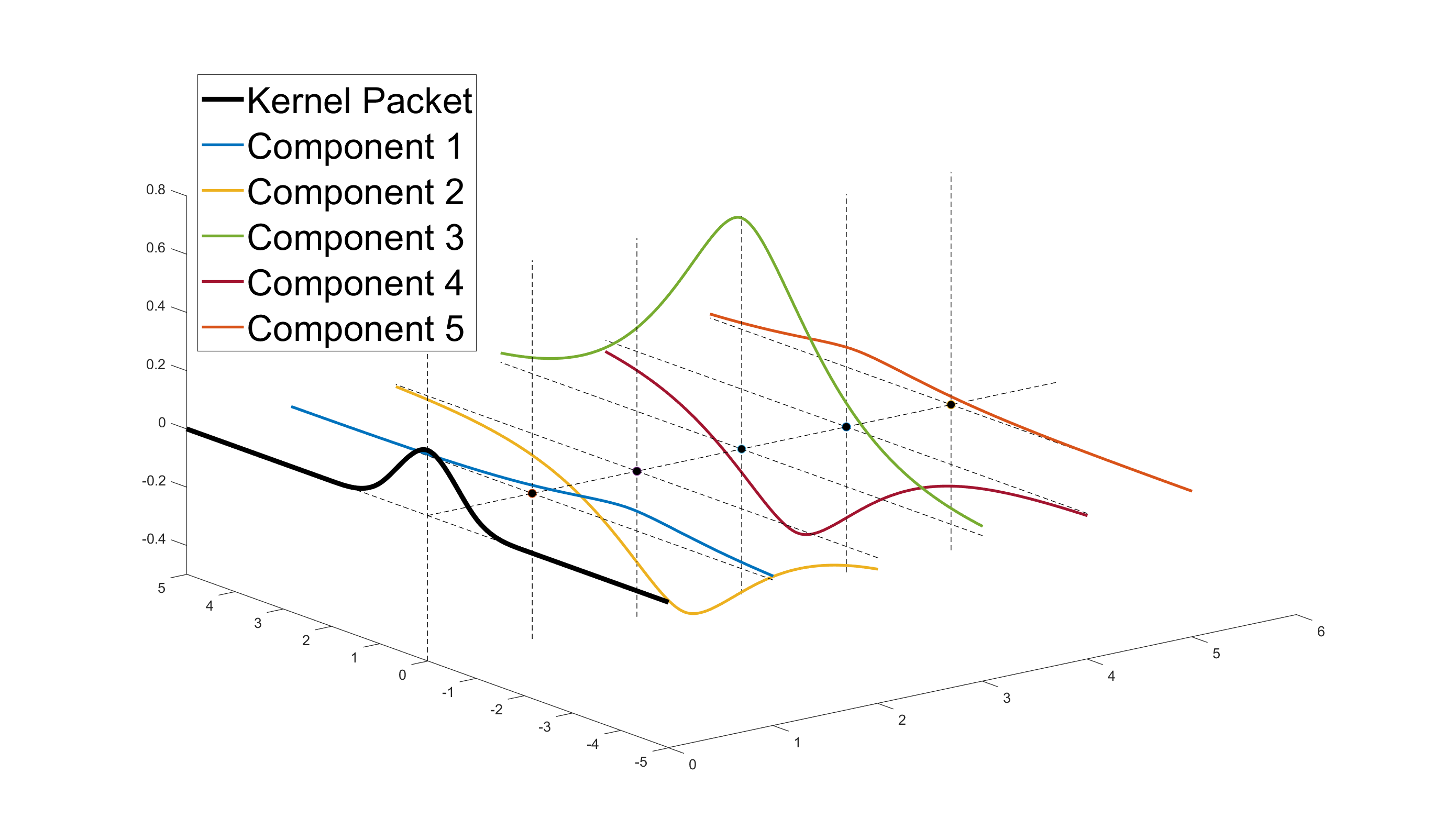
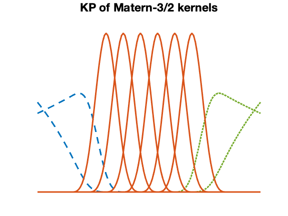
Figure 1: Left: the addition of five Matérn-$\frac{3}{2}$ kernels $a_{j}k(\cdot,x_{j})$ (colored lines, without compact supports) leads to a KP (black line, with a compact support); Right: converting 10 Matérn-$\frac{3}{2}$ kernel functions $\{k(\cdot,x_{i})\}_{i=1}^{10}$ to 10 KPs, where each KP is non-zeron on at most three points in $\{x_{i}\}_{i=1}^{10}$.

Theorem 4.1 (Chen et al. (2022))

Let $k$ be a Matérn-$\nu$ kernel with half-integer smoothness parameter $\nu$, i.e., $\nu=\frac{1}{2},\frac{3}{2},\cdots$. Let $(x_{1}<x_{2}<\cdots<x_{p})$ be any sorted one-dimensional points.

1. If $p=2\nu+2$, let $(a_{1},\cdots,a_{p})$ be the solution of the following system of equations:

   $$\sum_{i=1}^{p}a_{i}x_{i}^{l}\exp\{\delta cx_{i}\}=0,$$ (9)

   with $l=0,\ldots,(p-1)/2$, $c=2\nu\omega^{2}/(2\pi)^{2}$, and $\delta=\pm 1$. Then function: $\phi_{(x_{1},\cdots,x_{p})}=\sum_{i=1}^{p}a_{i}k(\cdot,x_{i})$ is non-zero only on interval $(x_{1},x_{p})$;

2. If $\nu+\frac{3}{2}\leq p<2\nu+2$, let $(a_{1},\cdots,a_{p})$ be the solution of the following system of equations

   $$\sum_{i=1}^{p}a_{i}x_{i}^{l}\exp\{hcx_{i}\}=0,\quad\sum_{i=1}^{p}a_{i}x_{i}^{r}\exp\{-hcx_{i}\}=0,$$ (10)

   where $l=0,\ldots,(2\nu-1)/2$, and the second term comprises auxiliary equations with $r=0,\ldots,p-\nu-5/2$ ( if $p-\nu-5/2<0$, skip the right side of (10) ). If $h=1$, then function: $\phi_{(x_{1},\cdots,x_{p})}=\sum_{i=1}^{p}a_{i}k(\cdot,x_{i})$ is non-zero only on interval $(-\infty,x_{p})$; If $h=-1$, then function: $\phi_{(x_{1},\cdots,x_{p})}=\sum_{i=1}^{p}a_{i}k(\cdot,x_{i})$ is non-zero only on interval $(x_{1},\infty)$.

Theorem 4.1 shows that for any $p$ sorted points $\{x_{i}\}_{i=1}^{p}$, there exists linear combination such that $\phi_{(x_{1},\cdots,x_{p})}=\sum_{i=1}^{p}a_{i}k(\cdot,x_{i})$ is non-zero only on $(x_{1},x_{p})$. Remind that the associated one-dimensional GP covariance matrix $k_{d}(\bm{X}_{d},\bm{X}_{d})$ can be viewed as the values of $n$ kernel functions $\{k(\cdot,x_{i})\}_{i=1}^{n}$ on $\{x_{i}\}_{i=1}^{n}$. We can convert these $n$ kernel functions to $n$ KPs and get the Gram matrix $\bm{\Phi}$ on $\{x_{i}\}_{i=1}^{n}$. Because each KP is non-zero only at $p$ points in $\{x_{i}\}_{i=1}^{n}$, $\bm{\Phi}$ must be a banded matrix. Algorithm 2 shows the factorization (8) explicitly.

Algorithm 2 Computing banded matrices $\bm{A}$ and $\bm{\Phi}$ such that $\bm{P}^{T}\bm{K}\bm{P}=\bm{A}^{-1}\bm{\Phi}$

Input: one-dimension Matérn-$\nu$ covariance matrix $\bm{K}$, scattered points $\{x_{i}\}_{i=1}^{n}$
      Output: banded matrices $\bm{A}$ and $\bm{\Phi}$, and permutation matrix $\bm{P}$

$\nu$ is a half-integer, $n\geq 2\nu+2$

Initialize $\bm{A},\bm{\Phi}\leftarrow\bm{0}\in\mathbb{R}^{n\times n}$

search permutation $\bm{P}$ to sort $\{x_{i}\}_{i=1}^{n}$ in increasing order

for $i=1$ to $\nu+\frac{1}{2}$ do

     Compute $\{a_{l}\}_{l=1}^{i+\nu+1/2}$ associated to $\{x_{l}\}_{l=1}^{i+\nu+1/2}$ via (10) with $h=1$

     $[\bm{A}]_{1:i+\nu+1/2,i}\leftarrow(a_{1},\cdots,a_{i+\nu+\frac{1}{2}})$ 

end for

for $i=\nu+3/2$ to $n-\nu-\frac{1}{2}$ do

     Compute $\{a_{l}\}_{l=1}^{2\nu+2}$ associated to $\{x_{l}\}_{l=i-\nu-1/2}^{i+\nu+1/2}$ via (9)

     $[\bm{A}]_{i-\nu-1/2:i+\nu+1/2,i}\leftarrow(a_{1},\cdots,a_{2\nu+2})$ 

end for

for $i=n-\nu+\frac{1}{2}$ to $n$ do

     Compute $\{a_{l}\}_{l=1}^{n-i+\nu+3/2}$ associated to $\{x_{l}\}_{l=i-\nu-1/2}^{n}$ via (10) with $h=-1$

     $[\bm{A}]_{i-\nu-1/2:n,i}\leftarrow(a_{1},\cdots,a_{n-i+\nu+3/2})$ 

end for

$\bm{\Phi}=\bm{A}\bm{P}^{T}\bm{K}\bm{P}$

We can analyze the time and space complexity of Algorithm 2. Firstly, sorting $n$ points in increasing order requires $\mathcal{O}(n\log n)$ time complexity. Secondly, the total $n$ iterations requires $\mathcal{O}(n)$ time complexity, as each iteration of the algorithm involves solving a $p\times p$ system of equations, which has a time complexity of $\mathcal{O}(1)$. We can also see that the matrices $\bm{A}$ is of band widths $\nu+1/2$ since at most $2\nu+2$ entries on the $i$-th row of $\bm{A}$ are flipped to non-zero in the $i$-th iteration. At last, the matrix $\bm{\Phi}$ is a $\nu-1/2$-banded matrix for the $i$-th row of $\Phi$ equals to the value of a KP on $\{x_{i}\}_{i=1}^{n}$, which has at most $2\nu$ non-zero entries. Therefore, the time and space complexity for computing $\bm{\Phi}=\bm{A}\bm{K}$ are both $\mathcal{O}(n)$. To summarize, the total time and space complexity of Algorithm 2 are $\mathcal{O}(n\log n)$ and $\mathcal{O}(n)$, respectively.

4.2 Derivative of Covariance Matrix

In this subsection, we generalized the theory of KP in Chen et al. (2022) to show that for any Matérn kernel with half-integer smoothness parameter $\nu$ and any $p=2\nu+4$ sorted points $\{x_{i}\}_{i=1}^{p}$, there exists linear combination such that

$$\psi_{(x_{1},\cdots,x_{p})}(x)=\sum_{i=1}^{p}b_{i}{\partial_{\omega}k(\omega|x-x_{i}|)}$$

is non-zero only on interval $(x_{1},x_{p})$. As a result, $\partial_{\omega}k_{d}(\omega|\bm{X}_{d}-\bm{X}_{d}|)$, the derivative of any one-dimensional Matérn covariance matrix with respective to the scale hyperparameter $\omega$, can also be factorized as product of a banded patrix $\bm{\Psi}_{d}$ and the inverse of a banded matrix $\bm{B}_{d}$:

$$\bm{P}_{d}^{T}\big{[}\partial_{\omega}k_{d}(\omega|\bm{X}_{d}-\bm{X}_{d}|)\big{]}\bm{P}_{d}=\bm{B}_{d}^{-1}\bm{\Psi}_{d}$$ (11)

where $\bm{X}_{d}$ is any one-dimensional point set, $\bm{P}_{d}$ is the permutation that sorts $\bm{X}_{d}$ in increasing order, and the band widths of both $\bm{\Psi}_{d}$ and $\bm{B}_{d}$ are $\nu+1/2$ and $\nu+3/2$, respectively.

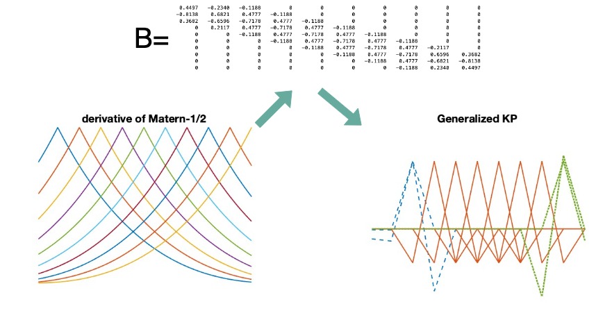
Figure 2: derivative of kernel functions: $\{{\partial_{\omega}k(\cdot,i/10)}\}_{i=1}^{10}$ can be converted to compactly support generalized KPs via a banded matrix $\bm{A}$

Figure 2 illustrates how to convert $\partial_{\omega}k_{d}(\omega|\bm{X}_{d}-\bm{X}_{d}|)$, the derivative of Matérn-$\frac{1}{2}$ matrix, with $\omega=1$ and $\bm{X}_{d}=\{.1,\cdots,1\}$ to the banded matrix $\bm{\Psi}_{d}$ via a specific banded matrix $\bm{B}$. The $(i,j)$-entry of $\partial_{\omega}k_{d}(\omega|\bm{X}_{d}-\bm{X}_{d}|)$ is equal to $\partial_{\omega}k_{d}(\omega|x_{i}-x_{j}|)=-|x_{i}-x_{j}|exp\{-|x_{i}-x_{j}|\}$ and, hence, the derivative matrix is dense. On the other hand, the $(i,j)$-entry of $\bm{\Psi}_{d}$ is equal to the value of generalized KP at $x_{j}$: $\psi_{(x_{i-2},x_{i-1},x_{i},x_{i+1},x_{i+2})}(x_{j})$. Therefore, $[\bm{\Psi}]_{i,j}$ is equal to $0$ if $|i-j|\geq 2$ because in this case $x_{j}$ is out of the support of generalize KP $\psi_{(x_{i-2},x_{i-1},x_{i},x_{i+1},x_{i+2})}$.

The construction of generalized KPs for the derivative of the Matérn kernel is very similar, except we treat the derivative of a Matérn-$\nu$ kernel as a Matérn-$(\nu+1)$ kernel and use Theorem 4.1 to compute the coefficients. The coefficients for constructing the KPs of the Matérn-$(\nu+1)$ kernel are also the coefficients for constructing the generalized KPs of the derivative of the Matérn-$\nu$ kernel. Formal theories are left in Appendix. We directly show Algorithm 3 for construction the sparse matrix factorization (11). The time and space complexity of Algorithm 3 are exactly the same as Algorithm 2, which is $\mathcal{O}(n\log n)$. We use the following theorem to summarize Algorithm 3.

Theorem 4.2

Let $\bm{\Psi}$, $\bm{B}$ be the outputs of Algorithm 3. Then $\bm{\Psi}$ is a $\nu+\frac{1}{2}$-banded matrix and $\bm{B}$ is a $\nu+\frac{3}{2}$-banded matrix. Moreover, for any set of scattered point $\{x_{i}\}_{i=1}^{n}$, $\bm{B}$ is invertable.

Algorithm 3 Computing banded matrices $\bm{B}$ and $\bm{\Psi}$ such that $\partial_{\omega}\bm{K}_{\omega}=\bm{B}^{-1}\bm{\Phi}$

Input: derivative of Matérn-$\nu$ covariance matrix $\partial_{\omega}\bm{K}_{\omega}$, scattered points $\{x_{i}\}_{i=1}^{n}$
      Output: banded matrices $\bm{B}$ and $\bm{\Psi}$, and permutation matrix $\bm{P}$

$\nu$ is a half-integer, $n\geq 2\nu+4$

Initialize $\bm{B},\bm{\Psi}\leftarrow\bm{0}\in\mathbb{R}^{n\times n}$

run Algorithm 2 for Matérn-$(\nu+1)$ covariance matrix on scatered points $\{x_{i}\}_{i=1}^{n}$

$\bm{P}$ is the output $\bm{P}$ of Algorithm 2

$\bm{B}\leftarrow\bm{A}$ where $\bm{A}$ is the output of Algorithm 2

$\bm{\Phi}=\bm{B}\bm{P}^{T}\partial_{\omega}\bm{K}_{\omega}\bm{P}$

In the following content, we will see that computing the gradient $\partial_{\omega}l$, we only need the banded matrices $\{\bm{\Psi}_{d}\}_{d=1}^{D}$ and $\{\bm{B}^{-1}_{d}\}_{d=1}^{D}$ associated to one-dimensional covariance matrices $\{\bm{K}_{d}\}$. Therefore, Theorem 4.2 guarantees that all the computations and banded solvers applied are feasible.

5 Fast Computation

As described in Hastie et al. (2009), Gilboa et al. (2013), the backfitting algorithm is a widely used approach for fitting additive models in high-dimensional spaces. In this algorithm, the additive model is constructed by fitting individual univariate nonparametric regression models to each variable in the $D$-dimensional input space. The backfitting algorithm iteratively refines these models by alternately updating the fit for each variable while holding the others fixed. Each iteration of the backfitting algorithm involves solving a set of univariate regression problems, which can be done efficiently with methods like kernel smoothing or least squares regression. For polynomial smoothers or Gauss-Markov models, each iteration requires $\mathcal{O}(n)$ time complexity. However, current backfittig algorithms for additive GPs are only for prediction, i.e., computing the posterior mean in (1). To the best of our knowledge, direct application of backfitting algorithm on computing the posterior variance in (1), the log-likelihood function $l$ in (5) and its gradient in (6) is still unknown.

Our algorithms, which are essentially based on iterative method, can compute the posterior mean, posterior variance, the log-likelihood $l$, and the gradient of $l$ efficiently. Before presenting our algorithm, we first directly substitute sparse factorization (8) into (4) and (5), and substitute sparse factorization (11) into(6) to rewrite them in the following forms:

$$\mu_{n}(\bm{x}^{*})=\bm{1}^{T}\bm{\phi}^{T}({\bm{x}^{*}})\bm{\Phi}^{-T}\bm{P}^{T}[\bm{P}\bm{\Phi}^{-1}\bm{A}\bm{P}^{T}+\frac{1}{\sigma_{y}^{2}}\bm{S}\bm{S}^{T}]^{-1}\bm{S}(\frac{1}{\sigma_{y}^{2}}\bm{\mathrm{I}}_{n})\bm{Y}$$ (12)

$$s_{n}(\bm{x}^{*})=\sum_{d=1}^{D}k_{d}(x^{*}_{d},\bm{x}^{*}_{d})-\sum_{d=1}^{D}\bm{\phi}^{T}_{d}(x^{*}_{d})\bm{\Phi}_{d}^{-T}\bm{A}_{d}^{-1}\bm{\phi}_{d}(x^{*}_{d})$$

$$\quad\quad+\bm{1}^{T}\bm{\phi}^{-T}({\bm{x}^{*}})\bm{\Phi}^{-T}\bm{P}^{T}[\bm{P}\bm{\Phi}^{-1}\bm{A}\bm{P}^{T}+\frac{1}{\sigma_{y}^{2}}\bm{S}\bm{S}^{T}]^{-1}\bm{P}\bm{\Phi}^{-1}\bm{\phi}({\bm{x}^{*}})\bm{1}$$ (13)

$$l(\bm{\omega},\sigma_{y})\propto\frac{\bm{Y}}{D}^{T}\bm{S}^{T}\bm{P}\bm{A}_{\bm{\theta}}^{T}\bm{\Phi}_{\bm{\theta}}^{-T}\bm{P}^{T}[\bm{P}\bm{\Phi}_{\bm{\theta}}^{-1}\bm{A}_{\bm{\theta}}\bm{P}^{T}+\frac{1}{\sigma_{y}^{2}}\bm{S}\bm{S}^{T}]^{-1}\bm{P}\bm{\Phi}_{\bm{\theta}}^{-1}\bm{A}_{\bm{\theta}}\bm{P}^{T}\bm{S}\frac{\bm{Y}}{D}$$

$$\quad\quad-\frac{\bm{Y}}{D}^{T}\bm{S}^{T}\bm{P}\bm{A}_{\bm{\theta}}^{T}\bm{\Phi}_{\bm{\theta}}^{-T}\bm{P}^{T}\bm{S}\frac{\bm{Y}}{D}-\log|\bm{\Phi}_{\bm{\theta}}^{-1}\bm{A}_{\bm{\theta}}+\frac{1}{\sigma_{y}^{2}}\bm{S}\bm{S}^{T}|$$

$$\quad\quad-\log|\bm{\Phi}_{\bm{\theta}}|+\log|\bm{A}_{\bm{\theta}}|-2n\log\sigma_{y}$$ (14)

$$\frac{\partial l}{\partial\omega_{d}}\propto\bm{Y}^{T}R\bm{B}_{d}^{-1}\bm{\Psi}_{d}R\bm{Y}-\text{Trace}\left[R\bm{B}_{d}^{-1}\bm{\Psi}_{d}\right]$$ (15)

where

$$\bm{\Phi}=\begin{bmatrix}\bm{\Phi}_{1}&&\\ &\ddots&\\ &&\bm{\Phi}_{D}\end{bmatrix},\quad\bm{A}=\begin{bmatrix}\bm{A}_{1}&&\\ &\ddots&\\ &&\bm{A}_{D}\end{bmatrix},\quad\bm{P}=\begin{bmatrix}\bm{P}_{1}&&\\ &\ddots&\\ &&\bm{P}_{D}\end{bmatrix}\in\mathbb{R}^{Dn\times Dn}$$

$$\bm{\phi}(\bm{x}^{*})=\bm{A}\bm{\gamma}_{\bm{x}^{*}}=\begin{bmatrix}\bm{\phi}_{1}(x^{*}_{1})&&\\ &\ddots&\\ &&\bm{\phi}_{D}(x^{*}_{D})\end{bmatrix}\in\mathbb{R}^{Dn\times D},$$

$$R=\frac{1}{\sigma_{y}^{2}}\bm{\mathrm{I}}_{n}-\frac{1}{\sigma_{y}^{2}}\bm{S}^{T}[\bm{P}\bm{\Phi}^{-1}\bm{A}\bm{P}^{T}+\frac{1}{\sigma_{y}^{2}}\bm{S}\bm{S}^{T}]^{-1}\bm{S}\frac{1}{\sigma_{y}^{2}},$$

$\{\bm{P}_{d}\}$ are the permutation matrices, $\{\bm{\Phi}_{d}\}$ and $\{\bm{A}_{d}\}$ are the banded matrices in factorization (8) for one-dimensional GP covariance matrix $k_{d}(\bm{X}_{d},\bm{X}_{d})$, $\{\bm{\Psi}_{d}\}$ and $\{\bm{B}_{d}\}$ are the banded matrices in factorization (11), $\bm{\phi}_{d}(x_{d}^{*})=\bm{A}_{d}k_{d}(\bm{X}_{d},x^{*}_{d})$ are values of KPs at the $d$-th dimension of input point $\bm{x}^{*}$, and $\bm{\Phi}_{\bm{\theta}}$ and $\bm{A}_{\bm{\theta}}$ are the $\bm{\Phi}$ and $\bm{A}$ induced by hyperparameters $\bm{\theta}$, respectively. The factorizations in (12),(13),(14), and (15) play key roles in our algorithms. In the following content, we first introduce the training part of our our algorithm and then the prediction part.

5.1 Training

In the training part, we propose a fast algorithm for matrix inverse and a fast algorithm for matrix determinant. We first introduce the algorithm for matrix inverse then the algorithm for matrix determinant.

5.1.1 Matrix Inverse

In the training part, all computations involving matrix inverse are among one of the following three operations

1. Computing vector $\bm{b}_{\bm{v}}=\bm{T}^{-1}\bm{v}$ for vector $\bm{v}$ where $\bm{T}$ is banded matrix $\bm{\Phi}$ or $\bm{B}_{d}$;

2. compute the inverse matrix $\bm{M}:=[\bm{P}\bm{\Phi}^{-1}\bm{A}\bm{P}^{T}+\frac{1}{\sigma_{y}^{2}}\bm{S}\bm{S}^{T}]^{-1}$;

3. compute vector $\bm{b}_{\bm{v}}:=[\bm{P}\bm{\Phi}^{-1}\bm{A}\bm{P}^{T}+\frac{1}{\sigma_{y}^{2}}\bm{S}\bm{S}^{T}]^{-1}\bm{v}$ for any vector $\bm{v}$ ;

4. compute the $(\nu+\frac{1}{2})$-band of matrix $\bm{\Phi}_{d}^{-T}\bm{A}_{d}^{-1}$ for $d=1,\cdots,D$ .

Operation 1 can be done in $\mathcal{O}(n)$ time by applying banded matrix solver. For example, the algorithm based on the LU decomposition in Davis (2006) can be applied to solve the equation $\bm{T}^{-1}\bm{b}=\bm{v}$ in $\mathcal{O}(n)$ time, where $\bm{b}$ is the unknown. MATLAB provides convenient and efficient builtin functions, such as mldivide or decomposition, to solve sparse banded linear system in this form.

Operation 2 and 4 are not necessary in many situations. However, if we want to reduce the computation time of $s_{n}(\bm{x}^{*})$ from $\mathcal{O}(n\log n)$to $\mathcal{O}(\log n)$ for randomly selected $\bm{x}^{*}$ after training, full knowledge of $\bm{M}$ and the $(\nu+\frac{1}{2})$-band of matrix $\bm{\Phi}_{d}^{-T}\bm{A}_{d}^{-1}$ must be given. For predetermined predictive point $\bm{x}^{*}$, operation 2 and 4 can be skipped and only operation 3 and 4 will involve in the whole computation process, which requires $\mathcal{O}(n\log n)$ time in total. The reason for operation 4 is that only the $(\nu+\frac{1}{2})$-band of matrix $\bm{\Phi}_{d}^{-T}\bm{A}_{d}^{-1}$ is required in the later prediction part.

Algorithm 4 Computing vector $\tilde{\bm{v}}:=[\bm{P}\bm{\Phi}^{-1}\bm{A}\bm{P}^{T}+\frac{1}{\sigma_{y}^{2}}\bm{S}\bm{S}^{T}]^{-1}\bm{v}$

Input: permutation matrices $\{\bm{P}_{d}\}_{d=1}^{D}$, banded matrices $\{\bm{\Phi}_{d}\}_{d=1}^{D}$ and $\{\bm{A}_{d}\}_{d=1}^{D}$, vector $\bm{v}$, observational noise variance $\sigma_{y}^{2}$
      Output: vector $\tilde{\bm{v}}$

Initialize $\tilde{\bm{v}}_{d}^{(0)}\leftarrow\bm{0}\in\mathbb{R}^{n}$, $d=1,\cdots,D$

for $t=1$ to $T$ do

     

$$\tilde{\bm{v}}_{d}^{(t+1)}=\bm{P}_{d}^{T}\bm{\Phi}_{d}[\sigma_{y}^{2}\bm{A}_{d}+\bm{\Phi}_{d}]^{-1}\bm{P}_{d}\left(\frac{1}{\sigma_{y}^{2}}\bm{v}_{d}-\sum_{d^{\prime}<d}\tilde{\bm{v}}_{d^{\prime}}^{(t+1)}-\sum_{d^{\prime}>d}\tilde{\bm{v}}_{d^{\prime}}^{(t)}\right)$$ (16)

     where $\bm{v}_{d}$ denotes the $(dn-n+1)$-th entry to the $dn$-th entry of $\bm{v}$

end for

return $\tilde{\bm{v}}=[\tilde{\bm{v}}_{d}^{(T)}]_{d}$

Fast computations of operation 2 and 3 rely on Algorithm 4. Algorithm 4 is based on the Gauss-Seidel method (Davis 2006) for computing the vector $\tilde{\bm{v}}=[\bm{K}+\sigma_{y}^{-2}\bm{S}\bm{S}^{T}]^{-1}\bm{v}$. What we have done is to decompose the following iterative step into block matrix operations:

$$\quad\begin{bmatrix}\sigma_{y}^{2}\bm{K}_{1}^{-1}+\bm{\mathrm{I}}_{n}&&&&\\ \bm{\mathrm{I}}_{n}&\sigma_{y}^{2}\ \bm{K}_{2}^{-1}+\bm{\mathrm{I}}_{n}&&&\\ \vdots&&&\ddots&\\ \bm{\mathrm{I}}_{n}&\cdots&&\bm{\mathrm{I}}_{n}&\sigma_{y}^{2}\bm{K}_{1}^{-1}+\bm{\mathrm{I}}_{n}\end{bmatrix}\tilde{\bm{v}}^{(t+1)}$$

$$=\sigma_{y}^{-2}\bm{v}-\begin{bmatrix}\bm{0}&\bm{\mathrm{I}}_{n}&\bm{\mathrm{I}}_{n}&\cdots&\bm{\mathrm{I}}_{n}\\ \bm{0}&\bm{0}&\bm{\mathrm{I}}_{n}&\cdots&\bm{\mathrm{I}}_{n}\\ &&\ddots&&\\ &&&&\bm{0}\end{bmatrix}\tilde{\bm{v}}^{(t)}.$$ (17)

Compared with direct Gauss-Seidel (17), the improvement in the iterative step (16) is that it can be computed in $\mathcal{O}(n)$ time complexity since $[\sigma_{y}^{2}\bm{A}_{d}+\bm{\Phi}_{d}]$ is a banded matrix and we can apply the banded matrix solver in operation 1 to compute (17) .

In practice,the number of iterations required in Algorithm 4 is far less than the number of data and usually set in the order of $\mathcal{O}(\log n)$ or even $\mathcal{O}(1)$ (Saatçi 2012). As a result, the over time complexity of Algorithm 4 is $\mathcal{O}(n)$.

Operation 3 can be computed directly by applying Algorithm 4 on associated vector. Inverse matrix $\bm{M}$ in operation 2 can be computed by applying Algorithm 4 on vectors $\bm{e}_{1},\cdots,\bm{e}_{n}$ where $\bm{e}_{i}$ is a zero vector with $1$ on its $i$-th entry. The $i$-th column of $\bm{M}$ is exactly the output of Algorithm 4 with input $\bm{e}_{i}$, i.e.,

$$\bm{M}_{:,i}=[\bm{P}\bm{\Phi}^{-1}\bm{A}\bm{P}^{T}+\frac{1}{\sigma_{y}^{2}}\bm{S}\bm{S}^{T}]^{-1}\bm{e}_{i}.$$

Because we need to apply Algorithm 4 $n$ times for computing matrix $\bm{M}$, the computational time complexity for operation 2 is $\mathcal{O}(n^{2})$.

Algorithm 5 Computing the $(\nu+\frac{1}{2})$-band of $\bm{\Phi}^{-T}_{d}\bm{A}_{d}^{-1}$

Input: banded matrices $\bm{\Phi}_{d}$ and $\bm{A}_{d}$
      Output: $[\bm{\Phi}^{-T}_{d}\bm{A}_{d}^{-1}]_{i,j}$ for $|i-j|\leq\nu+\frac{1}{2}$

Define matrix blocks $\bm{H}_{i}^{-},\bm{H}_{i},\bm{H}_{i}^{+}$ of $[h_{i,j}]:=\bm{A}_{d}\bm{\Phi}_{d}^{T}$ as

$$\bm{H}_{i}^{-}= \begin{bmatrix}h_{s_{i},s_{i}-2\nu}&\cdots&h_{s_{i},s_{i}-1}\\ &\ddots&\vdots\\ &&h_{s_{i+1}-1,s_{i}-1}\end{bmatrix},$$

$$\bm{H}_{i}= \begin{bmatrix}h_{s_{i},s_{i}}&\cdots&h_{s_{i},s_{i+1}-1}\\ \vdots&\ddots&\vdots\\ h_{s_{i+1}-1,s_{i}}&\cdots&h_{s_{i+1}-1,s_{i+1}-1}\end{bmatrix},$$

$$\bm{H}_{i}^{+}= \begin{bmatrix}h_{s_{i},s_{i+1}}&&\\ \vdots&\ddots&\\ h_{s_{i+1}-1,s_{i+1}}&\cdots&h_{s_{i+1}-1,s_{i+2}-1}\end{bmatrix}$$ (18)

where $i=1,\cdots,I$, $I=\lceil\frac{n}{2\nu}\rceil$, $s_{i}=(i-1)2\nu+1$, and $s_{I+1}-1=\min\{n,2\nu I\}$

$\triangleright$ $\bm{A}_{d}\bm{\Phi}_{d}^{T}$ is a $2\nu$-banded matrix, and $\bm{H}_{1}^{-}$ and $\bm{H}_{I}^{+}$ are null

Define matrix blocks $\bm{M}_{i}^{-},\bm{M}_{i},\bm{M}_{i}^{+}$ of $\bm{\Phi}^{-T}_{d}\bm{A}_{d}^{-1}$ corresponding to the same entry indices of $\bm{H}_{i}^{-},\bm{H}_{i},\bm{H}_{i}^{+}$

Solve $\bm{M}_{1}$, $\bm{M}_{1}^{+}$

for $j=2$ to $I$ do

     $\bm{M}_{j}^{-}=\bm{M}_{j-1}^{+}$ $\triangleright$ $\bm{A}_{d}\bm{\Phi}_{d}^{T}=\bm{A}_{d}\bm{K}_{d}\bm{A}^{T}_{d}$ is a symmetric matrix

     Solve auxiliary matrix $\bm{M}_{j}^{--}$:

$$\bm{H}_{j-1}^{-}\bm{M}_{j-2}+\bm{H}_{j-1}\bm{M}_{j-1}^{-}+\bm{H}_{j-1}^{+}\bm{M}_{j}^{--}=\bm{0}$$

$\triangleright$ skip for $j=2$

     Solve $\bm{M}_{j}:\bm{M}_{j}^{--}\bm{H}_{j-1}^{-}+\bm{M}_{j}^{-}\bm{H}_{j-1}+\bm{M}_{j}\bm{H}_{j-1}^{+}=\bm{0}$

     Solve $\bm{M}_{j}^{+}:\bm{M}_{j}^{-}\bm{H}_{j}^{-}+\bm{M}_{j}\bm{H}_{j}+\bm{M}_{j}^{+}\bm{H}_{j}^{+}=\bm{\mathrm{I}}_{2\nu}$ $\triangleright$ skip for $j=I$

end for

return $\bm{M}_{j}^{-},\bm{M}_{j},\bm{M}_{j}^{+},j=1,\cdots I$

Algorithm 5 is designed to perform operation 4 in $\mathcal{O}(\nu^{2}n)$ time. The main concept behind Algorithm 5 is that the multiplication of a $(\nu+1/2)$-banded matrix with a $(\nu-1/2)$-banded matrix results in a $2\nu$-banded matrix, which can be partitioned into a block-tridiagonal matrix $\bm{H}=\text{diag}[\bm{H}^{-}_{j},\bm{H}_{j},\bm{H}^{+}_{j}]$, where each block is a $2\nu$-by-$2\nu$ matrix. Since we only require the $(\nu+1/2)$-band of $\bm{\Phi}^{-T}_{d}\bm{A}_{d}^{-1}$, we can utilize the block-tridiagonal property of $\bm{H}$. This means that the multiplication of any row/column of $\bm{\Phi}^{-T}_{d}\bm{A}_{d}^{-1}$ by any column/row of $\bm{H}$ only involves three consecutive $2\nu$-by-$2\nu$ block matrices from $\bm{\Phi}^{-T}_{d}\bm{A}_{d}^{-1}$. The process of computing the band of $\bm{\Phi}^{-T}_{d}\bm{A}_{d}^{-1}$ is illustrated in Figure 3. Solving a $2\nu$-by-$2\nu$ matrix equation has a time complexity of $O(\nu^{3})$, and since we only need to solve $O(n/\nu)$ of these matrix equations, the total time complexity of Algorithm 5 is $O(\nu^{2}n)$.

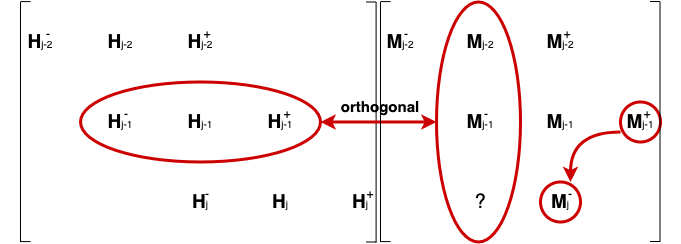
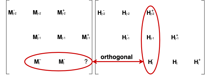
Figure 3: The time complexity of calculating any block matrix is $\mathcal{O}(\nu^{3})$, provided that it can be placed in a consecutive row/column with two other known block matrices. This is because $\bm{H}$ is a block-tridiagonal matrix. When working on the $j$-th column, we can get $\bm{M}_{j}^{-}=\bm{M}_{j-1}^{+}$ directly by symmetry and solve an auxiliary matrix $\bm{M}_{j}^{--}$ by putting $[\bm{M}_{j-2};\bm{M}_{j-1}^{-};\bm{M}_{j}^{--}]$ in a consecutive column (left); then we can first put $[\bm{M}_{j}^{--},\bm{M}_{j}^{-},\bm{M}_{j}]$ to solve $\bm{M}_{j}$ (middle), and then put $[\bm{M}_{j}^{-},\bm{M}_{j},\bm{M}_{j}^{+}]$ to solve $\bm{M}_{j}^{+}$ (right).

5.1.2 Matrix Determinant and Trace

Remind that for learning the hyperparameter, we must also compute the log-likelihood function (14) and its gradient (15), which involve computing matrix inverse, matrix determinants and matrix trace. All Matrix inversions in (14) and (15) can be computed by using Algorithm (4) and banded matrix solver. We also need to compute the following terms:

$$\log|\bm{\Phi}_{\bm{\theta}}^{-1}\bm{A}_{\bm{\theta}}+\frac{1}{\sigma_{y}^{2}}\bm{S}\bm{S}^{T}|,\quad\log|\bm{\Phi}_{\bm{\theta}}|,\quad\log|\bm{A}_{\bm{\theta}}|,\quad\text{Trace}\left[R\bm{B}_{d}^{-1}\bm{\Psi}_{d}\right].$$

The log determinant terms $\log|\bm{\Phi}_{\bm{\theta}}|$ and $\log|\bm{A}_{\bm{\theta}}|$ can also be computed in $\mathcal{O}(\nu^{2}n)$ time because both $\bm{A}_{\bm{\theta}}$ and $\bm{\Phi}_{\bm{\theta}}$ are $\nu+1/2$-banded matrix and $\nu-1/2$-banded matrix, respectively, and their determinants can be computed in $\mathcal{O}(\nu^{2}n)$ time by sequential methods (Kamgnia and Nguenang 2014).

For $\log|\bm{\Phi}_{\bm{\theta}}^{-1}\bm{A}_{\bm{\theta}}+\frac{1}{\sigma_{y}^{2}}\bm{S}\bm{S}^{T}|$, we first estimate its largest eigenvalue, and then we utilize the Taylor expansion of matrix log determinant to design an iterative method that resembles Algorithm 4, which enables us to estimate its value.

Algorithm 6 [Power Method] Computing the largest eigenvalue of $\bm{\Phi}_{\bm{\theta}}^{-1}\bm{A}_{\bm{\theta}}+\frac{1}{\sigma_{y}^{2}}\bm{S}\bm{S}^{T}$

Input: matrix $\bm{\Phi}_{\bm{\theta}}^{-1}\bm{A}_{\bm{\theta}}+\frac{1}{\sigma_{y}^{2}}\bm{S}\bm{S}^{T}$
      Output: largest eigenvalue of $\bm{\Phi}_{\bm{\theta}}^{-1}\bm{A}_{\bm{\theta}}+\frac{1}{\sigma_{y}^{2}}\bm{S}\bm{S}^{T}$

Initialize $\lambda_{\max}\leftarrow\bm{0}\in\mathbb{R}^{Dn}$

for $q=1$ to $Q$ do

     Initialize ${\bm{v}}^{(0)}$: each entry of ${\bm{v}}^{(0)}$ is uniformly distributed on $\{-1,1\}$

     for $s=1$ to $S$ do

         

$${\bm{v}}^{(s)}=[\bm{\Phi}_{\bm{\theta}}^{-1}\bm{A}_{\bm{\theta}}+\frac{1}{\sigma_{y}^{2}}\bm{S}\bm{S}^{T}]{\bm{v}}^{(s-1)}$$ (19)

     end for

     $\lambda=[\bm{v}^{(S)}]^{T}[\bm{\Phi}_{\bm{\theta}}^{-1}\bm{A}_{\bm{\theta}}+\frac{1}{\sigma_{y}^{2}}\bm{S}\bm{S}^{T}]{\bm{v}}^{(S)}/\|\bm{v}^{(S)}\|^{2}$

     If $\lambda>\lambda_{max}$: $\lambda_{\max}\leftarrow\lambda$

end for

return $\lambda_{max}$

To estimate the largest eigenvalue of $\bm{\Phi}_{\bm{\theta}}^{-1}\bm{A}_{\bm{\theta}}+\frac{1}{\sigma_{y}^{2}}\bm{S}\bm{S}^{T}$, we can simply use the power method Mises and Pollaczek-Geiringer (1929) as shown in Algorithm 6. Because both $\bm{\Phi}_{\bm{\theta}}$ and $\bm{A}_{\bm{\theta}}$ are banded matrices, (19) in each iteration can be computed in $\mathcal{O}(n)$ time using LU decomposition as discussed before. The number of iterations required in Algorithm 6 is independent of the data size $n$ for power method is essentially a Monte Carlo method.

After we estimate the largest eigenvalue of $\bm{\Phi}_{\bm{\theta}}^{-1}\bm{A}_{\bm{\theta}}+\frac{1}{\sigma_{y}^{2}}\bm{S}\bm{S}^{T}$, we can normalize it to a positive definite matrix with eigenvalue less than 1 and then apply the following Taylor expansion of log determinant to the normalized matrix:

$$\log|M|=-\sum_{s=1}^{\infty}\frac{1}{s}\text{trace}\left((\bm{\mathrm{I}}-M)^{s}\right)$$ (20)

where $M$ is any positive definite matrix with all eigenvalues less than $1$. The basic idea of computing the log determinant of $\bm{\Phi}_{\bm{\theta}}^{-1}\bm{A}_{\bm{\theta}}+\frac{1}{\sigma_{y}^{2}}\bm{S}\bm{S}^{T}$ numerically is to use a truncation of (20). The key ingredient for fast computation of (20) is efficient computation of the trace $\text{trace}\left((\bm{\mathrm{I}}-M)^{s}\right)$. Algorithm (7) in Avron and Toledo (2011) is a randomized algorithm for computing the trace of any symmetric positive definite (SPD) matrix. It has been proved in Avron and Toledo (2011) that the total number of iterations $Q$ required for a certain level of precision is independent of matrix size $n$. So time complexity of Algorithm 7 only depends on the time complexity for computing matrix multiplication (23).

Algorithm 7 [Avron and Toledo (2011)] Computing the trace of a matrix $\bm{M}$

Input: any SPD matrix $\bm{M}\in\mathbb{R}^{n\times n}$
      Output: trace of $\bm{M}$

$\gamma\leftarrow 0$

for $q=1$ to $Q$ do

     Initialize $\bm{v}_{q}\sim\mathcal{N}(0,\bm{\mathrm{I}}_{n})$

     

$$\gamma\leftarrow\bm{v}_{q}^{T}\bm{M}\bm{v}_{q}+\gamma$$ (21)

end for

$\gamma\leftarrow\frac{\gamma}{Q}$

return $\gamma$

Algorithm 8 combines Algorithm 6 and Algorithm 7 to numerically compute the log determinant of a matrix. The inner iteration number $S$ is in fact the truncated order of the Taylor expansion (20):

$$\log|\frac{1}{\lambda_{max}}\left(\bm{\Phi}_{\bm{\theta}}^{-1}\bm{A}_{\bm{\theta}}+\frac{1}{\sigma_{y}^{2}}\bm{S}\bm{S}^{T}\right)|\approx-\sum_{s=1}^{S}\frac{1}{s}\text{trace}\left(\frac{\bm{\Phi}_{\bm{\theta}}^{-1}\bm{A}_{\bm{\theta}}+\frac{1}{\sigma_{y}^{2}}\bm{S}\bm{S}^{T}}{\lambda_{max}}\right)$$ (22)

and the outer iteration number $Q$ is the number of samples for estimating the trace of a matrix. It has been proved in Boutsidis et al. (2017) that the truncation (22) converges to the true value exponential fast in truncation point $S$. Therefore, only $S=\mathcal{O}(\log n)$ is required for the inner iteration in Algorithm 8. Remind that $Q$ is independent of data size $n$ and (23) can be computed in $\mathcal{O}(n)$ time by banded matrix solver, Algorithm 8 require $\mathcal{O}(n\log n)$ time.

Algorithm 8 Computing $\log|\bm{\Phi}_{\bm{\theta}}^{-1}\bm{A}_{\bm{\theta}}+\frac{1}{\sigma_{y}^{2}}\bm{S}\bm{S}^{T}|$

Input: matrix $\bm{\Phi}_{\bm{\theta}}^{-1}\bm{A}_{\bm{\theta}}+\frac{1}{\sigma_{y}^{2}}\bm{S}\bm{S}^{T}$
      Output: $\log|\bm{\Phi}_{\bm{\theta}}^{-1}\bm{A}_{\bm{\theta}}+\frac{1}{\sigma_{y}^{2}}\bm{S}\bm{S}^{T}|$

use Algorithm 6 to estimate $\lambda_{max}$, the largest eigenvalue of $\bm{\Phi}_{\bm{\theta}}^{-1}\bm{A}_{\bm{\theta}}+\frac{1}{\sigma_{y}^{2}}\bm{S}\bm{S}^{T}$

$\bm{M}\leftarrow\bm{\mathrm{I}}_{Dn}-\frac{1}{\lambda_{max}}\left(\bm{\Phi}_{\bm{\theta}}^{-1}\bm{A}_{\bm{\theta}}+\frac{1}{\sigma_{y}^{2}}\bm{S}\bm{S}^{T}\right)$

$\gamma\leftarrow 0$

for $q=1$ to $Q$ do

     Initialize $\bm{v}_{0}\sim\mathcal{N}(0,\bm{\mathrm{I}}_{Dn})$

     for $s=1$ to $S$ do

         

$$\bm{v}_{s}=\bm{M}\bm{v}_{s-1}$$ (23)

         $\gamma\leftarrow\frac{1}{s}\bm{v}_{0}^{T}\bm{v}_{s}+\gamma$

     end for

end for

$\gamma\leftarrow nD\log\lambda_{max}-\frac{\gamma}{Q}$

return $\gamma$

For computing the trace term $\text{Trace}\left[R\bm{B}_{d}^{-1}\bm{\Psi}_{d}\right]$, we can directly use Algorithm 7. For any $\bm{v}_{q}$ in (21), we have

$$\bm{v}_{q}^{T}R\bm{B}_{d}^{-1}\bm{\Psi}_{d}\bm{v}_{q}=\frac{\bm{v}_{q}^{T}\bm{B}_{d}^{-1}\bm{\Psi}_{d}\bm{v}_{q}}{\sigma_{y}^{2}}-\frac{\bm{v}^{T}}{\sigma_{y}^{2}}\bm{S}^{T}[\bm{P}\bm{\Phi}^{-1}\bm{A}\bm{P}^{T}+\frac{1}{\sigma_{y}^{2}}\bm{S}\bm{S}^{T}]^{-1}\bm{S}\frac{\bm{B}_{d}^{-1}\bm{\Psi}_{d}\bm{v}_{q}}{\sigma_{y}^{2}}$$ (24)

The first term of (24) can be computed in $\mathcal{O}(n)$ using banded matrix solver. For the second term, we can first use bander matrix solver to get $\bm{B}_{d}^{-1}\bm{\Psi}_{d}\bm{v}_{q}$ and then use Algorithm 4, which take $\mathcal{O}(n)\log n$ time in total. Also, the number of iterations $Q$ in Algorithm 7 is independent of $n$ and, hence, the time complexity for computing the trace is $\mathcal{O}(n\log n)$

To summarize, the log determinant terms $\log|\bm{\phi}_{\bm{\theta}}|$ and $\log|\bm{A}_{\bm{\theta}}|$ can both be computed in $\mathcal{O}(\nu^{2}n)$ time using LU decomposition algorithm, while $\log|\bm{\Phi}_{\bm{\theta}}^{-1}\bm{A}_{\bm{\theta}}+\frac{1}{\sigma_{y}^{2}}\bm{S}\bm{S}^{T}|$ can be computed in $\mathcal{O}(n\log n)$ time using Algorithm 8 and $\text{Trace}\left[R\bm{B}_{d}^{-1}\bm{\Psi}_{d}\right]$ can be computed in $\mathcal{O}(n\log n)$ using Algoritm 7. Therefore, the total time complexity for computing all the determinant terms in the log-likelihood function (14) and its gradient is $\mathcal{O}(n\log n)$.

5.2 Prediction

Because the support of KP $[\bm{\phi}_{d}]_{i}$ is $(x_{i-\nu-1/2,d},x_{i+\nu+1/2,d})$ for any $i=1,\cdots,n$ and $d=1,\cdots,D$, so, for any predictive point $\bm{x}^{*}$ and dimension $d$, there must be at most $2\nu+1$ non-zero entries on $\bm{\phi}_{d}(x^{*}_{d})$ and these non-zero entries are also consecutive. This fact is the essential idea for fast computation of prediction. For a given $x^{*}_{d}$, searching the $2\nu+1$ consecutive non-zero entries on $\bm{\phi}_{d}(x^{*}_{d})$ is equivalent to searching the sorted data point $x_{i,d}$ such that $x_{i,d}<x^{*}_{d}<x_{i+1,d}$, which requires $\mathcal{O}(\log n)$ time complexity only.

For fixed hyperhyparameter $\bm{\theta}$ and predetermined predictive point $\bm{x}^{*}$, we can skip operation 2 and do operation 3 and 3 only in the training. In this case, we can first use Algorithm 4 and fast banded matrix solver to compute vectors $\bm{b}_{\bm{v}_{1}}:=\bm{\Phi}^{-T}\bm{P}^{T}[\bm{P}\bm{\Phi}^{-1}\bm{A}\bm{P}^{T}+\frac{1}{\sigma_{y}^{2}}\bm{S}\bm{S}^{T}]^{-1}\bm{S}(\frac{1}{\sigma_{y}^{2}}\bm{\mathrm{I}}_{n})\bm{Y}$ and $\bm{b}_{\bm{v}_{2}}:=\bm{\Phi}^{-T}\bm{P}^{T}[\bm{P}\bm{\Phi}^{-1}\bm{A}\bm{P}^{T}+\frac{1}{\sigma_{y}^{2}}\bm{S}\bm{S}^{T}]^{-1}\bm{P}\bm{\Phi}^{-1}\bm{\phi}({\bm{x}^{*}})$ in $\mathcal{O}(n\log n)$ time. For $\mu_{n}(\bm{x}^{*})$ in (12), because $\mu_{n}(\bm{x}^{*})$ equals sparse vector multiplication $\bm{1}^{T}\bm{\phi}^{T}({\bm{x}^{*}})\bm{b}_{\bm{v}_{1}}$, the prediction part only required $\mathcal{O}(1)$ time complexity. For $s_{n}(\bm{x}^{*})$ in (13), the third term equals $\bm{1}^{T}\bm{\phi}^{T}({\bm{x}^{*}})\bm{b}_{\bm{v}_{2}}$, which is also sparse matrix multiplication and can be computed in $\mathcal{O}(1)$ time. For the third term, we first use Algorithm 5 to get the $\nu+\frac{1}{2}$-band of $\bm{\Phi}_{d}^{-T}\bm{A}_{d}^{-1}$ for $d=1,\cdots,D$. This operation requires $\mathcal{O}(n)$ time. Suppose the $2\nu+1$ consecutive non-zeros entries on $\bm{\phi}(\bm{x}^{*})$ are with indices $\{i_{d}^{*},i^{*}_{d}+1,\cdots,i^{*}+2\nu\}_{d=1}^{D}$, then the second term of $s_{n}(\bm{x}^{*})$ is

$$\quad\sum_{d=1}^{D}\bm{\phi}_{d}^{T}(x^{*}_{d})\bm{\Phi}_{d}^{-T}\bm{A}^{-1}_{d}\bm{\phi}_{d}(x^{*}_{d})$$

$$=\sum_{d=1}^{D}\sum_{j=0}^{2\nu}\sum_{l=0}^{2\nu}[\bm{\phi}_{d}(x^{*}_{d})]_{i_{d}^{*}+j}[\bm{\phi}_{d}(x^{*}_{d})]_{i_{d}^{*}+l}[\bm{\Phi}_{d}^{-T}\bm{A}^{-1}_{d}]_{i_{d}^{*}+j,i_{d}^{*}+l}.$$ (25)

Obviously, there are at $D4\nu^{2}$ additions in the (25), and, as a result, computation of the second term is also $\mathcal{O}(1)$.

To summarize, the total time complexity for the case that hyperparameters and predictive point are fixed before training, the overall time complexity is $\mathcal{O}(n\log n)$ because operation 3 and 3 in training only requires $\mathcal{O}(n\log n)$ time and, except for searching the non-zero entries on $\bm{\phi}(\bm{x}^{*})$, which requires $\mathcal{O}(\log n)$ time, every other step in prediction part only requires $\mathcal{O}(1)$ time.

However, in many application, hyperparameters and predictive point cannot be known before training. For example, in Bayesian optimization, we need to estimate the hyperparameter for the model and then search an optimal point based on the posterior. In this case, we must compute the matrix $\bm{M}$ and $\tilde{\bm{M}}$ in operation 2 of the training part. Although the time complexity for computing $\bm{M}$ and $\tilde{\bm{M}}$ is increased to $\mathcal{O}(n^{2})$ compared with the previous case, time complexity for prediction part remains unchanged. Notice that vector $\bm{b}_{\bm{v}_{1}}:=\bm{\Phi}^{-T}\bm{P}^{T}[\bm{P}\bm{\Phi}^{-1}\bm{A}\bm{P}^{T}+\frac{1}{\sigma_{y}^{2}}\bm{S}\bm{S}^{T}]^{-1}\bm{S}(\frac{1}{\sigma_{y}^{2}}\bm{\mathrm{I}}_{n})\bm{Y}$ is independent of predictive point $\bm{x}^{*}$ so computation of $\mu_{n}(\bm{x}^{*})$ remains unchanged. Also, the sparsity in (25) remains unchanged. The only difference is that we now need to compute the term $\bm{1}^{T}\bm{\phi}^{T}({\bm{x}^{*}})\tilde{\bm{M}}\bm{\phi}({\bm{x}^{*}})\bm{1}$ with out using Algorithm 4 for otherwise every prediction require $\mathcal{O}(n)$ time. Similary to (25), we can see that the computation of $\bm{\phi}^{T}({\bm{x}^{*}})\tilde{\bm{M}}\bm{\phi}({\bm{x}^{*}})$ only involves $4D^{2}\nu^{2}$ addition as follows:

$$\sum_{d,d^{\prime}=1}^{D}\bm{\phi}_{d}^{T}({x^{*}_{d}})\tilde{\bm{M}}_{d,d^{\prime}}\bm{\phi}_{d^{\prime}}({x^{*}_{d^{\prime}}})$$

where $[\tilde{M}_{d,d^{\prime}}]_{d,d^{\prime}}$ is the partition of $\tilde{\bm{M}}$ into $D\times D$ block matrices and for any $(d,d^{\prime})$

$$\quad\bm{\phi}_{d}^{T}(x^{*}_{d})\tilde{M}_{d,d^{\prime}}\bm{\phi}_{d^{\prime}}(x^{*}_{d^{\prime}})$$

$$=\sum_{j=0}^{2\nu}\sum_{l=0}^{2\nu}[\bm{\phi}_{d}(x^{*}_{d})]_{i^{*}_{d}+j}[\bm{\phi}_{d^{\prime}}(x^{*}_{d^{\prime}})]_{i_{d^{\prime}}^{*}+l}[\tilde{M}_{d,d^{\prime}}]_{i_{d}^{*}+j,i_{d^{\prime}}^{*}+l}.$$ (26)

To summarize, the total time complexity for unknown hyperparameters and predictive point is $\mathcal{O}(n^{2})$ because operation 2 and computing $\partial l/\partial\bm{\theta}$ involve multiplications of dense matrices, which at least requires $\mathcal{O}(n^{2})$ time. Nonetheless, every step in prediction part remains unchanged, which only requires $\mathcal{O}(1)$ time.

5.3 Summary

We have proposed different algorithms for computing different terms in the posterior mean (12), posterior variance (4), the log-likelihood (14) and its gradient (15). To summarize the efficient computation of additive GPs, we first list all the terms we need to compute and use a table to briefly review their efficient computations.

$$\mu_{n}(\bm{x}^{*})=\bm{1}^{T}\bm{\phi}^{T}({\bm{x}^{*}})\underbrace{\bm{\Phi}^{-T}\bm{P}^{T}[\bm{P}\bm{\Phi}^{-1}\bm{A}\bm{P}^{T}+\frac{1}{\sigma_{y}^{2}}\bm{S}\bm{S}^{T}]^{-1}\bm{S}(\frac{1}{\sigma_{y}^{2}}\bm{\mathrm{I}}_{n})\bm{Y}}_{\bm{b}_{\bm{Y}}}$$

$$s_{n}(\bm{x}^{*})=\sum_{d=1}^{D}k_{d}(x^{*}_{d},\bm{x}^{*}_{d})-\sum_{d=1}^{D}\bm{\phi}^{T}_{d}(x^{*}_{d})\underbrace{\bm{\Phi}_{d}^{-T}\bm{A}_{d}^{-1}}_{\nu+1/2\ \text{band}}\bm{\phi}_{d}(x^{*}_{d})$$

$$\quad\quad+\bm{1}^{T}\bm{\phi}^{-T}({\bm{x}^{*}})\underbrace{\bm{\Phi}^{-T}\bm{P}^{T}[\bm{P}\bm{\Phi}^{-1}\bm{A}\bm{P}^{T}+\frac{1}{\sigma_{y}^{2}}\bm{S}\bm{S}^{T}]^{-1}\bm{P}\bm{\Phi}^{-1}}_{\bm{M}}\bm{\phi}({\bm{x}^{*}})\bm{1}$$

$$l(\bm{\theta})\propto\underbrace{\frac{\bm{Y}}{D}^{T}\bm{S}^{T}\bm{P}\bm{A}_{\bm{\theta}}^{T}\bm{\Phi}_{\bm{\theta}}^{-T}\bm{P}^{T}[\bm{P}\bm{\Phi}_{\bm{\theta}}^{-1}\bm{A}_{\bm{\theta}}\bm{P}^{T}+\frac{1}{\sigma_{y}^{2}}\bm{S}\bm{S}^{T}]^{-1}\bm{P}\bm{\Phi}_{\bm{\theta}}^{-1}\bm{A}_{\bm{\theta}}\bm{P}^{T}\bm{S}\frac{\bm{Y}}{D}}_{\text{quad}-\mathcal{A}}$$

$$\quad\quad-\underbrace{\frac{\bm{Y}}{D}^{T}\bm{S}^{T}\bm{P}\bm{A}_{\bm{\theta}}^{T}\bm{\Phi}_{\bm{\theta}}^{-T}\bm{P}^{T}\bm{S}\frac{\bm{Y}}{D}}_{\text{quad}-\mathcal{B}}-\underbrace{\log|\bm{\Phi}_{\bm{\theta}}^{-1}\bm{A}_{\bm{\theta}}-\frac{1}{\sigma_{y}^{2}}\bm{S}\bm{S}^{T}|}_{\text{log\ det}-\mathcal{A}}$$

$$\quad\quad-\underbrace{\log|\bm{\Phi}_{\bm{\theta}}|}_{\text{log\ det}-\mathcal{B}}+\underbrace{\log|\bm{A}_{\bm{\theta}}|}_{\text{log\ det}-\mathcal{C}}-2n\log\sigma_{y}$$

$$\frac{\partial l}{\partial\bm{\theta}_{d}}\propto\underbrace{\bm{Y}^{T}R\bm{B}_{d}^{-1}\bm{\Psi}_{d}R\bm{Y}}_{\text{quad}-\mathcal{D}}-\underbrace{\text{Trace}\left[R\bm{B}_{d}^{-1}\bm{\Psi}_{d}\right]}_{\text{Trace}}.$$

Table 1: Summary of computations for the posterior and log-likelihood

Term	Algorithm	Time Complexity
$\bm{b}_{\bm{y}}$	Algorithm 4 and LU decomposition	$\mathcal{O}(n\log n)$
$\bm{\phi}^{T}(\bm{x}^{*})\bm{b}_{\bm{y}}$	sparse vector multiplication	$\mathcal{O}(1)$ if $\bm{b}_{\bm{y}}$ and non-zero entries on $\bm{\phi}(\bm{x}^{*})$ are known; $\mathcal{O}(\log n)$ if $\bm{b}_{\bm{y}}$ is known but non-zero entries on $\bm{\phi}(\bm{x}^{*})$ are unknown
$(\nu+1/2$)-band of $\bm{\Phi}^{-T}_{d}\bm{A}^{-1}_{d}$	Algorithm 5	$\mathcal{O}(\nu^{2}n)$
$\bm{\phi}_{d}^{T}(x^{*}_{d})\bm{\Phi}^{-T}_{d}$ $\cdot\bm{A}^{-1}_{d}\bm{\phi}_{d}(x^{*}_{d})$	Sparse vector multiplication or LU decomposition	$\mathcal{O}(1)$ if the $(\nu+1/2$)-band of $\bm{\Phi}^{-T}_{d}\bm{A}^{-1}_{d}$ and non-zero entries on $\bm{\phi}(\bm{x}^{*})$ are known; $\mathcal{O}(\log n)$ if the $(\nu+1/2$)-band of $\bm{\Phi}^{-T}_{d}\bm{A}^{-1}_{d}$ are known but non-zero entries on $\bm{\phi}(\bm{x}^{*})$ are unknown; $\mathcal{O}(n\log n)$ if the $(\nu+1/2$)- band of $\bm{\Phi}^{-T}_{d}\bm{A}^{-1}_{d}$ are unknown
$\bm{M}$	Algorithm 4 and LU decomposition	$\mathcal{O}(n^{2})$
$\bm{\phi}^{T}(\bm{x}^{*})\bm{M}\bm{\phi}(\bm{x}^{*})$	sparse vector multiplication or Algorithm 4	$\mathcal{O}(1)$ if $\bm{M}$ and non-zero entries on $\bm{\phi}(\bm{x}^{*})$ are known; $\mathcal{O}(\log n)$ if $\bm{M}$ is known but non-zero entries on $\bm{\phi}(\bm{x}^{*})$ is unknown; $\mathcal{O}(n\log n)$ if $\bm{M}$ is unknown
quad-$\mathcal{A},\mathcal{B}$	Algorithm 4 and LU decomposition	$\mathcal{O}(n\log n)$
log det-$\mathcal{A}$	Algorithms 6, 8, and LU decomposition	$\mathcal{O}(n\log n)$
log det-$\mathcal{B},\mathcal{C}$	sequential method in Kamgnia and Nguenang (2014)	$\mathcal{O}(\nu^{2}n)$
quad-$\mathcal{D}$	Algorithm 4 and LU decomposition	$\mathcal{O}(n\log n)$
Trace	Algorithm 4 and 7	$\mathcal{O}(n\log n)$

6 Application to Bayesian Optimization

In this section, we use the sparsity nature of KP $\bm{\phi}(\cdot)$ to design a fast algorithm for searching the next sampling point in Bayesian optimization, i.e., searching $\bm{x}=\arg\max_{\bm{x}}A(\bm{x},\bm{X},\bm{Y})$. In short, write $A:=A(\cdot,\bm{X},\bm{Y})$. We use GP-UCB as an example to explicitly demonstrate our algorithm. Our algorithm can also be applied to general acquisition function, such as EI, as we will discuss later. Remind that the acquisition function of GP-UCB is

$$A(\bm{x})=\mu_{n}(\bm{x})+\beta_{n}\sqrt{s_{n}(\bm{x})}$$ (27)

where, in our setting, $\mu_{n}$ is the posterior mean and $s_{n}$ is the posterior variance of an additive GP with Matérn covariance. Updating the posterior in Algorithm 1 can be done by the training procedure in Section 5.1. We mainly introduce the gradient method for searching the maximizaer.

From Section 5.2, (27) can be written in a sparse form for any predictive point $\bm{x}^{*}$:

$$A(\bm{x}^{*}) =\underbrace{\sum_{d=1}^{D}\sum_{i=i^{*}}^{i*+2\nu}\bm{b}_{i,d}[\bm{\phi}_{d}(x^{*}_{d})]_{i}}_{\mu_{n}(\bm{x}^{*})}$$

$$\quad+\beta_{n}\underbrace{\sqrt{\sum_{d,d^{\prime}=1}^{D}\sum_{i,j=i^{*}}^{i^{*}+2\nu}[\bm{\phi}_{d}(x^{*}_{d})]_{i}[\bm{\phi}_{d^{\prime}}(x^{*}_{d^{\prime}})]_{j}m_{i,j,d,d^{\prime}}}}_{\sqrt{s_{n}(\bm{x}^{*})}}$$ (28)

where $\bm{b}_{i,d}$ is the entry on vector $\bm{\Phi}^{-T}\bm{P}^{T}[\bm{P}\bm{\Phi}^{-1}\bm{A}\bm{P}^{T}+\frac{1}{\sigma_{y}^{2}}\bm{S}\bm{S}^{T}]^{-1}\bm{S}(\frac{1}{\sigma_{y}^{2}}\bm{\mathrm{I}}_{n})\bm{Y}$ corresponding to $[\bm{\phi}_{d}(x^{*}_{d})]_{i}$ on $\bm{\phi}(\bm{x}^{*})$ in vector multiplication and, similarly, $m_{i,j,d,d^{\prime}}$ is the entry on matrix $\bm{\Phi}^{-T}\bm{A}^{-1}+\bm{\Phi}^{-T}\bm{P}^{T}[\bm{P}\bm{\Phi}^{-1}\bm{A}\bm{P}^{T}+\frac{1}{\sigma_{y}^{2}}\bm{S}\bm{S}^{T}]^{-1}\bm{P}\bm{\Phi}^{-1}$ corresponding to $[\bm{\phi}_{d}(x^{*}_{d})]_{i}$ on $\bm{\phi}^{T}(\bm{x}^{*})$ and $[\bm{\phi}_{d^{\prime}}(x^{*}_{d^{\prime}})]_{j}$ on $\bm{\phi}(\bm{x}^{*})$ in the quadratic form. Remind that, for any $d$, there are only $\mathcal{O}(1)$ non-zero entries on KPs $\bm{\phi}_{d}(x_{d}^{*})$. As a result, computing the gradient of $A$ at $\bm{x}^{*}$ only requires $\mathcal{O}(1)$ operations

$$\frac{\partial A}{\partial x^{*}_{d}}= \frac{\partial\mu_{n}}{\partial x^{*}_{d}}+\beta_{n}\frac{\partial\sqrt{s_{n}}}{\partial x^{*}_{d}}$$ (29)

where

$$\frac{\partial\mu_{n}}{\partial x^{*}_{d}}=\sum_{i=i^{*}}^{i*+2\nu}\bm{b}_{i,d}\frac{\partial[\bm{\phi}_{d}(x^{*}_{d})]_{i}}{\partial x^{*}_{d}}$$

$$\frac{\partial\sqrt{s_{n}}}{\partial x^{*}_{d}}=\frac{1}{2\sqrt{s_{n}(\bm{x}^{*})}}\bigg{(}2\sum_{d=1}^{D}\sum_{i,j=i^{*}}^{i^{*}+2\nu}\frac{\partial[\bm{\phi}_{d}(x^{*}_{d})]_{i}}{\partial x^{*}_{d}}[\bm{\phi}_{d^{\prime}}(x^{*}_{d^{\prime}})]_{j}m_{i,j,d,d}$$

$$\quad\quad+\sum_{d\neq d^{\prime}}^{D}\sum_{i,j=i^{*}}^{i^{*}+2\nu}\frac{\partial[\bm{\phi}_{d}(x^{*}_{d})]_{i}}{\partial x^{*}_{d}}[\bm{\phi}_{d^{\prime}}(x^{*}_{d^{\prime}})]_{j}m_{i,j,d,d^{\prime}}\bigg{)}$$

and the gradient of a KP at $x_{d}^{*}$ is

$$\frac{\partial[\bm{\phi}_{d}(x^{*}_{d})]_{i}}{\partial x_{d}^{*}}=\sum_{j=i^{*}-\nu-\frac{1}{2}}^{i^{*}+\nu+1/2}[\bm{A}_{d}]_{j,i}\frac{\partial k_{d}(x_{j},x^{*}_{d})}{\partial x^{*}_{d}}.$$

Recall that $s_{n}(\bm{x}^{*})$ is summation of finite term in (28), we can see that the number of additions in (29) is independent of the total number of data $n$. The gradient of $\mu_{n}(\bm{x}^{*})$ and $s_{n}(\bm{x}^{*})$ can be written in the following more compact matrix forms:

$$\nabla_{\bm{x}^{*}}\mu_{n}(\bm{x}^{*})=\bm{g}_{\footnotesize\bm{\phi}}^{T}({\bm{x}^{*}})\bm{\Phi}^{-T}\bm{P}^{T}\bm{M}\bm{S}(\frac{1}{\sigma_{y}^{2}}\bm{\mathrm{I}}_{n})\bm{Y},$$

$$\nabla_{\bm{x}^{*}}s_{n}(\bm{x}^{*})=\bm{g}_{\footnotesize\bm{\phi}}^{T}({\bm{x}^{*}})\left[-\bm{\Phi}^{-T}\bm{A}^{-1}+2\bm{\Phi}^{-T}\bm{P}^{T}\bm{M}\bm{P}\bm{\Phi}^{-1}\right]\bm{g}_{\footnotesize\bm{\phi}}({\bm{x}^{*}})\bm{1},$$ (30)

where

$$\bm{g}_{\footnotesize\bm{\phi}}({\bm{x}^{*}})=\begin{bmatrix}{\partial_{x^{*}_{1}}}\bm{\phi}_{1}(x^{*}_{1})&&&\\ &{\partial_{x^{*}_{2}}}\bm{\phi}_{2}(x^{*}_{2})&&\\ &&\ddots&\\ &&&{\partial_{x^{*}_{D}}}\bm{\phi}_{D}(x^{*}_{D})\end{bmatrix}\in\mathbb{R}^{Dn\times D},$$

$$\bm{M}=[\bm{P}\bm{\Phi}^{-1}\bm{A}\bm{P}^{T}+\frac{1}{\sigma_{y}^{2}}\bm{S}\bm{S}^{T}]^{-1}\in\mathbb{R}^{Dn\times Dn},$$

vector ${\partial_{x^{*}_{d}}}\bm{\phi}_{d}(x^{*}_{d})$ consists of derivative of $d$-dimensional KPs $\bm{\phi}_{d}$ at $x^{*}_{d}$, and $\bm{1}=[1,\cdots,1]^{T}$ is a $D$-vector with all entries equal $1$. (30) can be derived directly by applying matrix derivative laws on (12) and (13). Please refer to Petersen et al. (2008) for matrix calculus in details. So the gradient of $A$ in matrix form is

$$\nabla_{\bm{x}^{*}}A(\bm{x}^{*})=\nabla_{\bm{x}^{*}}\mu_{n}(\bm{x}^{*})+\frac{\beta_{n}}{2\sqrt{s_{n}(\bm{x}^{*})}}\nabla_{\bm{x}^{*}}s_{n}(\bm{x}^{*}).$$

In general, an acquisition function $A(\bm{x}^{*})$ is a composition function of the form $A(\bm{x}^{*},\mu_{n}(\bm{x}^{*}),s_{n}(\bm{x}^{*}))$ because the Gaussian posterior can be fully determined by the posterior mean $\mu_{n}$ and posterior variance $s_{n}$. In this case, the gradient of $A$ is

$$\nabla_{\bm{x}^{*}}A=[\frac{\partial A}{\partial x^{*}_{1}},\cdots,\frac{\partial A}{\partial x^{*}_{D}}]^{T}+\frac{\partial A}{\partial\mu_{n}}\nabla_{\bm{x}^{*}}\mu_{n}(\bm{x}^{*})+\frac{\partial A}{\partial s_{n}}\nabla_{\bm{x}^{*}}s_{n}(\bm{x}^{*}).$$

Because the derivatives of $A$ with respective to $x^{*}_{d}$, $\mu_{n}$, and $s_{n}$ are all independent of data size $n$, they all can be computed in $\mathcal{O}(1)$ time. The gradient $\nabla_{\bm{x}^{*}}\mu_{n}(\bm{x}^{*})$ and $\nabla_{\bm{x}^{*}}s_{n}(\bm{x}^{*})$ can also be computed in $\mathcal{O}(1)$ time as discussed previously. We can conclude that for any acquisition function $A$, its gradient with respective to $\bm{x}^{*}$ can be computed in $\mathcal{O}(1)$ time if our method is applied.

Indeed, when using gradient method for searching the maximizer of $A$, the time complexity of computing the posterior at each updated point $\bm{x}^{**}=\bm{x}^{*}+\delta\nabla_{\bm{x}^{*}}A(\bm{x}^{*})$ can be further reduced to $\mathcal{O}(1)$ when the learning rate $\delta$ satisfies

$$\delta\|\nabla_{\bm{x}^{*}}A(\bm{x}^{*})\|\leq{C}{\min_{i,j,d}|x_{i,d}-x_{j,d}|}$$

where $C$ is some constant independent of $n$. In this case, the updated point $\bm{x}^{**}$ is not a randomly selected new predictive point but a point near $\bm{x}^{*}$. Remind that the supports of KPs $\{[\bm{\phi}_{d}]_{i}\}_{i=1}^{n}$ are consecutive, it is straightforward to derive that indices for non-zero entries on $\bm{\phi}_{d}(x^{**}_{d})$ are within the $C=\frac{\|\delta\nabla_{\bm{x}^{*}}A(\bm{x}^{*},\bm{X},\bm{Y})\|}{\min_{i,j,d}|x_{i,d}-x_{j,d}|}$-nearest neighbors of indices for non-zero entries on $\bm{\phi}_{d}(x^{*}_{d})$. As a result, we can search the non-zero entries on $\bm{\phi}_{d}(\bm{x}^{**}_{d})$ by looking at the approximately all the $C$-nearest neighbors of $\bm{x}^{*}$, which requires $\mathcal{O}(1)$ time only. In generally, computing the value of acquisition $A$ at $\bm{x}^{**}$ requires $\mathcal{O}(\log n)$ time. This is because we need to search the $x_{i,d}$ that is closet to $x^{**}_{d}$ for all dimension $d$ as we have explained in section 5.2.

7 Numerial Experiments

In this section, we run our algorithms on the following test functions for prediction and Bayesian optimization:

$$f_{\text{Schwefel}}(\bm{x})=418.9829-\frac{1}{d}\sum_{d=1}^{D}x_{d}\sin(\sqrt{|x_{d}|}),\quad\bm{x}\in(-500,500)^{D},$$ (31)

$$f_{\text{Rastr}}(\bm{x})=10-\frac{1}{D}\sum_{d=1}^{D}\left(x_{d}^{2}-10\cos(2\pi x_{d})\right)\bm{x}\in(-5.12,5.12)^{D},$$ (32)

where (31) is the Schwefel function and (32) is the Rastr function. Both of them are complex functions with many local minima and, hence, ideal test functions for salable data. Figure 4 shows the two-dimensional projections of our test functions. All the observations are corrupted by a standard normal noise, i.e., $\bm{y}=f(\bm{x})+\varepsilon$, $\varepsilon\sim\mathcal{N}(0,1)$, for all $\bm{x}$.

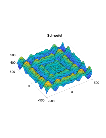
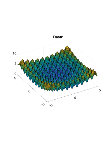
Figure 4: two-dimensional projections of ten-dimensional Schwefel (left) and Rastr (right)

We use Matérn-$\frac{1}{2}$ kernel for the covariance of GP:

$$k(\bm{x},\bm{x}^{\prime})=\sum_{d=1}^{D}\exp\left(-\theta|x_{d}-x_{d}^{\prime}|\right).$$

In this case, matrix $\bm{\Phi}$ is a diagonal matrix (with band width $0$) and matrix $\bm{A}$ is a tridiagonal matrix (with band width $3$) We first run our algorithm for prediction of ten and twenty dimensional Schwefel and Rastr functions conditioned on data of size up to $30000$. We then run our algorithm on GP-UCB for searching the global minimizer of five and ten dimensional Schwefel and Rastr functions with sampling budget up to $3000$.

All the experiments are implemented in Matlab (version 2018a) on a laptop computer with macOS, 3.3 GHz Intel Core i5 CPU, and 8 GB of RAM (2133 Mhz). The Matlab codes of the competing approaches are all publicly available.

7.1 Prediction

In this experiment, all the inputs $\bm{x}$ are uniformly generated from the domains of test function, i.e., $\bm{x}\sim\text{Unif}(-l,l)^{D}$ with $l=500,5.12$ and $D=10,20$. For dimension $D=10$, we examine our algorithm on all test functions with data size $n=3000,6000,\cdots,30000$. For dimension $D=20$, we examine our algorithm on all test functions with data size $n=2000,4000,\cdots,20000.$ We use our algorithms to first compute the scale parameter that maximizes the log-likelihood: $\omega^{*}=\max_{\omega>0}l(\omega)$. We then use our method to compute the posterior mean $\hat{f}$ on 100 randomly selected test points $\{\bm{x}_{i}^{*}\}_{i=1}^{100}$ and compute the following Root Mean Squared Error (RMSE) to test the performance of our method:

$$\text{RMSE}=\sqrt{\frac{1}{100}\sum_{i=1}^{100}[\hat{f}(\bm{x}^{*}_{i})-f(\bm{x}_{i}^{*})]^{2}}$$

where $f$ is the true test function. We repeated the experiments 100 times and recorded the standard deviation of the RMSE to test the stability of each prediction model:

$$\text{STD}=\sqrt{\frac{1}{100}\sum_{i=1}^{100}(\text{RMSE}-\overline{\text{RMSE}})^{2}}$$

where $\overline{\text{RMSE}}$ is the averaged RMSE over the 100 macro repetition. Averaged computational time for computing the MLE and prediction is also recorded. The following algorithms are used as benchmark:

1. Full GP (FGP) (Rasmussen and Williams 2006): naive implementation of GPs using GPML tool box.

2. Variational-Bayesian Expectation Maximization (VBEM) (Gilboa et al. 2013): a variational inference approach for approximation the log-likelihood and posterior variance of additive GP;

3. Inducing Points (IP): algorithm provided in the GPML tool box. The number of inducing points $m$ is set as $m=\sqrt{n}$, which is the choice to achieve the optimal approximation power for Matérn-$1/2$ correlation according to Burt et al. (2019).

We call our method generalized Kernel packet (GKP). The experimental results are shown in Figure 5.

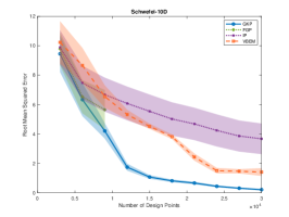
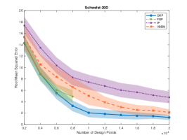
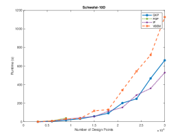
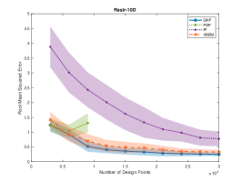
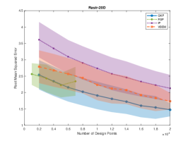
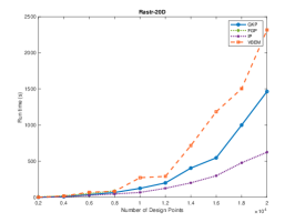
Figure 5: RMSE and computational time for test functions. The upper row corresponds to the Schwefel test function and the lower row corresponds to the Rastr test function. The three columns correspond to $d=10,20$ and computational time, respectively. The shaded areas areas represent standard deviation of the result

First, our approach GKP, in general, outperforms the others significantly in prediction accuracy. Not only does GKP yield the lowest RMSE in almost all the cases—regardless of the test function, dimensionality, or sample size—that are considered, but the corresponding STDs of RMSE also have the smallest widths. Because the STDs are calculated via multiple macro-replications in each of which a random set of prediction points are sampled, this suggests that the predictions given by GKP are more stable than the competing approaches.

Second, the right column in Figure 5 shows the average computational time of each approach in predicting the two test functions in different dimensions. Compared with the two approaches that are not based on matrix approximations (i.e., IP and VBEM) the advantage of GKP is clear, especially when the data size is large. However, compared with IP, the computational efficiency of GKP is lower but only by a small margin, especially when the sample size is large. This is not surprising because IP exploits low-rank approximations to accelerate matrix inversion. However, the acceleration in computation is achieved at the cost of prediction accuracy. Indeed, the RMSE associated with IP is markedly lower than that associated with both GKP and VBEM in almost all cases. In a nutshell, GKP achieves a much higher prediction accuracy with a slightly lower computational efficiency than the two approximation approaches.

7.2 Bayesion Optimization

In this experiment, we first randomly collect 100 sample points for the warm-up stage of Bayesian optimization algorithm. Then we use our algorithm GKP to compute the GP-UCB acquisition function for sequential samplings. At each sampling, we report the estimated minimizer of our algorithm. As a benchmark, we use full GP (FGP) to naively implement the GP-UCN algorithm. We set the search spaces as $(-500,500)^{D}$ with $D=10$ or $20$. In each iteration, we first learn the hyperparameter of the additive GP conditioned on current data. We then use our algorithms to search the point that maximizes the acquisition function of GP-UCB. At the end of each iteration, we samply noisy value at a point that maximized current acquisition function. For $D=10$, we set the simulation budget to be $N=300,6000,\cdots,30000$. For $D=20$, we set the simulation budget to be $N=2000,2000,\cdots,20000$. Note that both functions are minimized at $(420.9687,420.9687,\cdots,420.9687)$ and we have labeled the 2-D projection of the maximizer in the right column of 6.

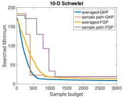
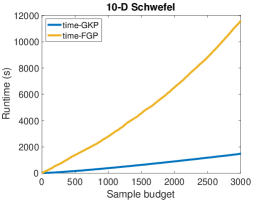
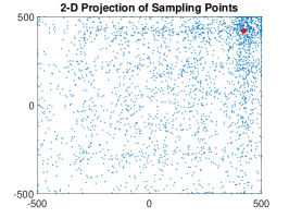
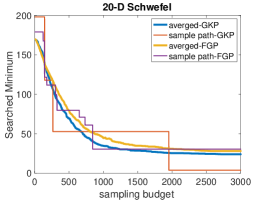
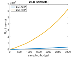
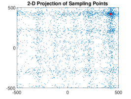
Figure 6: Searched Minimum, computational time, and sampling points. The upper row corresponds to the 10-dimensional Schwefel test function and the lower row corresponds to the 20-dimensional Schwefel test function. The left column is the minimum estimated by algorithms, the mideele is the computational times, the right column is the samples by GKP.

The results of our Bayesian optimization experiments are presented in Figure 6. Our algorithm, GKP, is shown to have higher computational accuracy due to its efficiency and sparsity. Moreover, our algorithm requires much lower time complexity. The left column of Figure 6 shows that GKP takes fewer iterations to estimate the minimizer, which, combined with the computational efficiency achieved by the sparsity of GKP, leads to its superior performance over FGP. As the data size increases during the sampling process, the advantage of GKP over FGP becomes even more evident. Finally, the right column of Figure 6 shows that GKP spends a large portion of the sampling budget around the true minimizer, which demonstrates the computational accuracy of our algorithm.

8 Conclusion

We present a novel approach to efficiently compute the posterior of an additive GP by decomposing it into a combination of one-dimensional GPs. Specifically, we leverage a recent development in sparse representation of one-dimensional Matérn GPs to represent the posterior of an additive GP as a formulation by sparse matrices. Our approach allows us to compute the posterior in $\mathcal{O}(n)$ time and, given the posterior, to compute any Bayesian optimization acquisition function and its associated gradient in $\mathcal{O}(\log n)$ or even $\mathcal{O}(1)$ time. We evaluate the performance of our algorithms on complex test functions with scalable data and demonstrate their effectiveness.

The current study can be extended in several ways, the first being the inference of additive GPs with sparse additive terms. While we have assumed a full additive model in our paper, some additive models (e.g., Raskutti et al. (2012), Cai and Pu (2022)) assume that there are only a small number of unknown effective additive terms. Therefore, our study can be extended to efficiently compute the inference of these effective terms. Secondly, it is worth noting that many current deep learning models can be viewed as compositions of additive models. As such, our proposed algorithms could be applied to efficient inference of these models, including deep Gaussian processes Damianou and Lawrence (2013) and Bayesian neural networks MacKay (1995), Neal (2012), Blundell et al. (2015). Finally, our current algorithms are only for additive GPs with Matérn covariances but we believe that our algorithms can be generalized to other commonly used covariances, such as integrated Brownian motion (Salemi et al. 2019), tensor Markov GPs Ding and Zhang (2022), and smoothing spline (Kimeldorf and Wahba 1970, Kim and Gu 2004).

9 Proof of Theorem 3.1

Proof 9.1

Proof. The intuition of (1) relies on representing the conditional distribution $\operatorname{\mathbb{P}}(\mathcal{G}(\bm{x}^{*})|\bm{X},\bm{Y})$ in the following form:

$$\quad\operatorname{\mathbb{P}}\left(\mathcal{G}(\bm{x}^{*})|\bm{X},\bm{Y}\right)$$

$$=\int\operatorname{\mathbb{P}}\left(\sum_{d=1}^{D}\mathcal{G}_{d}(x^{*}_{D})\bigg{|}\mathcal{G}_{1}(\bm{X}_{1}),\cdots,\mathcal{G}_{D}(\bm{X}_{D})\right)$$

$$\quad\cdot\operatorname{\mathbb{P}}\left(\mathcal{G}_{1}(\bm{X}_{1}),\cdots,\mathcal{G}_{D}(\bm{X}_{D})\bigg{|}\bm{Y}\right)d\mathcal{G}_{1}(\bm{X}_{1})\cdots d\mathcal{G}_{D}(\bm{X}_{D})$$

$$\propto\int\operatorname{\mathbb{P}}\left(\sum_{d=1}^{D}\mathcal{G}_{d}(x^{*}_{D})\bigg{|}\mathcal{G}_{1}(\bm{X}_{1}),\cdots,\mathcal{G}_{D}(\bm{X}_{D})\right)$$

$$\quad\cdot\operatorname{\mathbb{P}}\left(\bm{Y}|\mathcal{G}_{1}(\bm{X}_{1}),\cdots,\mathcal{G}_{D}(\bm{X}_{D})\right)\operatorname{\mathbb{P}}\left(\mathcal{G}_{1}(\bm{X}_{1}),\cdots,\mathcal{G}_{D}(\bm{X}_{D})\right)d\mathcal{G}_{1}(\bm{X}_{1})\cdots d\mathcal{G}_{D}(\bm{X}_{D})$$

where the first equality is from the formula of marginal distribution and the proportion relation is from Bayes rule. Remind that the $\mathcal{G}_{d}(\bm{X}_{d})$ above should be treated as a vector indexed by $\bm{X}_{d}$ instead of values of $\mathcal{G}_{d}$ on $\bm{X}_{d}$. To directly prove the theorem using the above identity involves long calculations. Therefore, we use algebraic calculations to show that the posterior variance in (4) is equivalent to the one in (1). Proof for the posterior mean is similarly.

Without loss of generality, assume $\sigma_{y}=1$, then

$$\bm{1}^{T}\bm{\gamma}_{\bm{x}^{*}}^{T}\bm{K}^{-1}[\bm{K}^{-1}+\bm{S}\bm{S}^{T}]^{-1}\bm{K}^{-1}\bm{\gamma}_{\bm{x}^{*}}\bm{1}$$

$$= \bm{1}^{T}\bm{\gamma}_{\bm{x}^{*}}^{T}\bm{K}^{-1}\left(\bm{K}-\bm{K}\bm{S}[\bm{\mathrm{I}}_{n}+\bm{S}^{T}\bm{K}\bm{S}]^{-1}\bm{S}^{T}\bm{K}\right)\bm{K}^{-1}\bm{\gamma}_{\bm{x}^{*}}\bm{1}$$

$$= \bm{1}^{T}\bm{\gamma_{\bm{x}^{*}}}^{T}\bm{K}^{-1}\bm{\gamma_{\bm{x}^{*}}}\bm{1}-\bm{1}^{T}\bm{\gamma}_{\bm{x}^{*}}^{T}\bm{S}[\bm{\mathrm{I}}_{n}+\bm{S}^{T}\bm{K}\bm{S}]^{-1}\bm{S}^{T}\bm{\gamma}_{\bm{x}^{*}}\bm{1}$$ (33)

where

$$[\bm{\mathrm{I}}_{n}+\bm{S}^{T}\bm{K}\bm{S}]^{-1}=\left[\sum_{d=1}^{D}k_{d}(\bm{X}_{d},\bm{X}_{d})+\bm{\mathrm{I}}_{n}\right]^{-1}$$

$$\bm{S}^{T}\bm{\gamma}_{\bm{x}^{*}}\bm{1}=\sum_{d=1}^{D}k_{d}(\bm{X}_{d},x^{*}_{d}).$$

Substitute (33) into (4), it is straightforward to check that (4) and (1) are equivalent.

10 Proof of Theorem 3.2

Proof 10.1

Proof. For (5), we can see in (2) that $l$ consists of the quadratic term and the log determinant term. For the quadratic term, we first use the following identity:

$$\quad\frac{\bm{Y}}{D}^{T}\bm{S}^{T}\bm{K}_{\bm{\theta}}^{-1}\left[\bm{K}_{\bm{\theta}}^{-1}+\sigma_{y}^{-2}\bm{S}\bm{S}^{T}\right]^{-1}\bm{K}_{\bm{\theta}}^{-1}\bm{S}\frac{\bm{Y}}{D}$$

$$=\frac{\bm{Y}}{D}^{T}\bm{S}^{T}\bm{K}_{\bm{\theta}}^{-1}\left(\bm{K}_{\bm{\theta}}-\bm{K}_{\bm{\theta}}\bm{S}\left[\bm{S}^{T}\bm{K}_{\bm{\theta}}\bm{S}+\sigma_{y}^{2}\bm{\mathrm{I}}_{n}\right]^{-1}\bm{S}^{T}\bm{K}_{\bm{\theta}}\right)\bm{K}_{\bm{\theta}}^{-1}\bm{S}\frac{\bm{Y}}{D}$$

$$=\frac{\bm{Y}}{D}^{T}\bm{S}^{T}\bm{K}_{\bm{\theta}}^{-1}\bm{S}\frac{\bm{Y}}{D}-\frac{\bm{Y}}{D}^{T}\bm{S}^{T}\bm{S}[\bm{S}^{T}\bm{K}_{\bm{\theta}}\bm{S}+\sigma^{2}\bm{\mathrm{I}}_{n}]^{-1}\bm{S}^{T}\bm{S}\frac{\bm{Y}}{D}$$ (34)

where the second line is from Woodbury matrix identity. Notice that

$$\frac{1}{D}\bm{S}^{T}\bm{S}\bm{Y}=\frac{1}{D}\sum_{d=1}^{D}\bm{Y}=\bm{Y}$$ (35)

So the quadratic term $\bm{Y}^{T}[k(\bm{X},\bm{X}|\bm{\theta}))+\sigma^{2}\bm{\mathrm{I}}_{n}]^{-1}\bm{Y}$ can be written as:

$$\quad\bm{Y}^{T}[k(\bm{X},\bm{X}|\bm{\theta})+\sigma^{2}\bm{\mathrm{I}}_{n}]^{-1}\bm{Y}$$

$$=\frac{\bm{Y}}{D}^{T}\bm{S}^{T}\bm{S}[\bm{S}^{T}\bm{K}_{\bm{\theta}}\bm{S}+\sigma^{2}\bm{\mathrm{I}}_{n}]^{-1}\bm{S}^{T}\bm{S}\frac{\bm{Y}}{D}$$

$$=\frac{\bm{Y}}{D}^{T}\bm{S}^{T}\bm{K}_{\bm{\theta}}^{-1}\bm{S}\frac{\bm{Y}}{D}-\frac{\bm{Y}}{D}^{T}\bm{S}^{T}\bm{K}_{\bm{\theta}}^{-1}\left[\bm{K}_{\bm{\theta}}^{-1}+\sigma_{y}^{-2}\bm{S}\bm{S}^{T}\right]^{-1}\bm{K}_{\bm{\theta}}^{-1}\bm{S}\frac{\bm{Y}}{D}$$

where the second line is from (35) and the third line is from (34). The above equation gives the quadratic term in (5).

For the log determinant term, we can use the matrix determinant lemma:

$$|\bm{S}^{T}\bm{K}_{\bm{\theta}}\bm{S}+\sigma_{y}^{2}\bm{\mathrm{I}}_{n}|=|\bm{K}_{\bm{\theta}}^{-1}+\sigma_{y}^{-2}\bm{S}\bm{S}^{T}|\cdot|\bm{K}_{\bm{\theta}}|\cdot|\sigma_{y}^{2}\bm{\mathrm{I}}_{n}|$$ (36)

which gives exactly the log determinant terms of (5).

For (6), we can use matrix derivative rules and apply Woodbury matrix identity to directly get the result.

11 Generalized Kernel Packet

The derivative of a Matérn kernel with half-integer smoothness parameter $\nu$ is of the following form:

$$k(x,x^{\prime}|\omega)=\sigma\exp({-{\omega}{|x-x^{\prime}|}})\frac{q!}{2q!}\left(\sum_{l=0}^{q}\frac{(q+l)!}{l!(q-l)!}({2\omega}{|x-x^{\prime}|})^{q-l}\right)$$ (37)

where $q=\nu-\frac{1}{2}$. Without loss of generality, we let $\sigma=1$. We first present the following theorem as a generalized version of 1 in Theorem 4.1.

Theorem 11.1 (Central )

Let $k(\cdot,\cdot|\omega)$ be a Matérn-$\nu$ kernel with half-integer $\nu$ and $q=\nu-1/2$. For any $p=2\nu+4$ points sorted in increasing order $\{x_{i}\}_{i=1}^{p}$, let $(b_{1},\cdots,b_{p})$ be the solution of the following system of equations:

$$\sum_{i=1}^{p}b_{i}x_{i}^{l}\exp(\delta\omega x_{i})=0,$$ (38)

with $l=0,\ldots,q+1$, and $\delta=\pm 1$. Then function: $\psi_{(x_{1},\cdots,x_{p})}=\sum_{i=1}^{p}b_{i}\partial_{\omega}k(\cdot,x_{i}|\omega)$ is non-zero only on interval $(x_{1},x_{p})$.

Proof 11.2

Proof. For any $x<x_{1}<x_{2}<\cdots,x_{p}$, we have

$$\partial_{\omega}k(x,x_{i}|\omega) =\partial_{\omega}\left(\exp\left({{\omega}(x-x_{i})}\right)\frac{q!}{2q!}\left(\sum_{l=0}^{q}\frac{(q+l)!}{l!(q-l)!}({2\omega}(x_{i}-x))^{q-l}\right)\right)$$

$$=(x-x_{i})\exp({{\omega}(x-x_{i})})\frac{q!}{2q!}\left(\sum_{l=0}^{q}\frac{(q+l)!}{l!(q-l)!}({2\omega}(x_{i}-x))^{q-l}\right)$$

$$\quad+\exp({{\omega}(x-x_{i})})\frac{q!}{2q!}\left(\sum_{l=0}^{q-1}\frac{(q+l)!}{l!(q-l-1)!}(2x_{i}-2x)^{q-l}\omega^{q-l-1}\right)$$

$$=-\exp(\omega(x-x_{i}))\frac{q!}{2q!}\sum_{s=2}^{q}\frac{(2q-s)!}{(q-s+1)!(s-2)!}(2\omega)^{s-1}(x_{i}-x)^{s}$$

$$\quad-\exp(\omega(x-x_{i}))\frac{q!2^{q}\omega^{q}}{2q!}(x_{i}-x)^{q+1}$$ (39)

where the first summation in (39) equals $0$ if $q\leq 1$. We can only consider the case $q\geq 2$. For $q\leq 1$, analysis i similar. When $q\geq 2$, (39) can be unified as

$$\partial_{\omega}k(x,x_{i}|\omega) =-\exp(\omega(x-x_{i}))\frac{q!}{2q!}\sum_{s=2}^{q+1}\frac{(2q-s)!}{(q-s+1)!(s-2)!}(2\omega)^{s-1}(x_{i}-x)^{s}$$

$$=-\exp(\omega(x-x_{i}))\frac{q!}{2q!}\sum_{s=2}^{q+1}\sum_{l=0}^{s}\frac{(2q-s)!}{(q-s+1)!(s-2)!}(2\omega)^{s-1}\frac{s!}{l!(s-l)!}x_{i}^{l}(-x)^{s-l}$$

$$=-\exp(\omega(x-x_{i}))\frac{q!}{2q!}\sum_{t=0}^{q+1}x_{i}^{l}\sum_{s=\max\{l,2\}}^{q+1}\frac{(2q-s)!}{(q-s+1)!(s-2)!}(2\omega)^{s-1}\frac{s!}{l!(s-l)!}(-x)^{s-l}$$

$$\coloneqq\sum_{l=0}^{q+1}x_{i}^{l}\exp(\omega(x-x_{i}))C(x,q,l)$$ (40)

where $C(x,q,t)$ in (40) is independent of $x_{i}$. Then for for any $\{b_{i}\}_{i=1}^{p}$ satisfying (38), we have

$$\psi_{(x_{1},\cdots,x_{p})}(x) =\sum_{i=1}^{p}b_{i}\partial_{\omega}k(x,x_{i}|\omega)$$

$$=\sum_{i=1}^{p}b_{i}\sum_{l=0}^{q+1}x_{i}^{l}\exp(\omega(x-x_{i}))C(x,q,l)$$

$$=\sum_{l=0}^{q+1}e^{\omega x}C(x,q,l)\sum_{i=1}^{p}b_{i}x_{i}^{l}e^{-\omega x_{i}}=0$$ (41)

where the second line is from (40) and the third line is from condition (38).

Similarly, for any $x>x_{p}>\cdots>x_{1}$, we have the identity

$$\partial_{\omega}k(x,x_{i}|\omega) =\partial_{\omega}\left(\exp\left({{\omega}(x_{i}-x)}\right)\frac{q!}{2q!}\left(\sum_{l=0}^{q}\frac{(q+l)!}{l!(q-l)!}({2\omega}(x-x_{i}))^{q-l}\right)\right)$$

$$=\sum_{l=0}^{q+1}x_{i}^{l}\exp(\omega(x_{i}-x))C^{\prime}(x,q,l)$$ (42)

and the same calculation as (41) shows

$$\psi_{(x_{1},\cdots,x_{p})}(x) =\sum_{l=0}^{q+1}e^{-\omega x}C^{\prime}(x,q,l)\sum_{i=1}^{p}b_{i}x_{i}^{l}e^{\omega x_{i}}=0.$$ (43)

Putting (41) and (43) together, we can have the final result.

The following Theorem is the generalization of 2 in Theorem 4.1.

Theorem 11.3 (One-sided)

Let $k(\cdot,\cdot|\omega)$ be a Matérn-$\nu$ kernel with half-integer $\nu$ and $q=\nu-1/2$. For any $p$ points sorted in increasing order $\{x_{i}\}_{i=1}^{p}$ with $\nu+\frac{5}{2}\leq p<2\nu+4$, let $(b_{1},\cdots,b_{p})$ be the solution of the following system of equations

$$\sum_{i=1}^{p}b_{i}x_{i}^{l}\exp\{h\omega x_{i}\}=0,\quad\sum_{i=1}^{p}b_{i}x_{i}^{r}\exp\{-h\omega x_{i}\}=0,$$ (44)

where $l=0,\ldots,q+1$, and the second term comprises auxiliary equations with $r=0,\ldots,p-\nu-7/2$ (if $p-\nu-7/2<0$, skip the right side of (44)). If $h=1$, then function: $\psi_{(x_{1},\cdots,x_{p})}=\sum_{i=1}^{p}b_{i}\partial_{\omega}k(\cdot,x_{i}|\omega)$ is non-zero only on interval $(-\infty,x_{p})$; If $h=-1$, then function: $\psi_{(x_{1},\cdots,x_{p})}=\sum_{i=1}^{p}b_{i}\partial_{\omega}k(\cdot,x_{i}|\omega)$ is non-zero only on interval $(x_{1},\infty)$.

Proof 11.4

Proof. We can use reasoning similar to the proof for Theorem 11.1. For any $x<x_{1}<\cdots<x_{p}$, according to (40),

$$\partial_{\omega}k(x,x_{i}|\omega)=\sum_{l=0}^{q+1}x_{i}^{l}\exp(\omega(x-x_{i}))C(x,q,l).$$

For any $\{b_{i}\}_{i=1}^{p}$ satisfying (44) with $h=-1$, we immediately have

$$\psi_{(x_{1},\cdots,x_{p})}(x)=\sum_{i=1}^{p}b_{i}\partial_{\omega}k(x,x_{i}|\omega)=\sum_{l=0}^{q+1}e^{\omega x}C(x,q,l)\sum_{i=1}^{p}b_{i}x_{i}^{l}e^{-\omega x_{i}}=0.$$

For any $x>x_{p}>\cdots>x_{1}$, we only need to switch the sign of $x$ and $x_{i}$ to get the final result.

Theorem 11.1 and 11.3 are exactly the same as Theorem 4.1 except that the coefficients $\{b_{i}\}_{i=1}^{p}$ for $\partial_{\omega}k(\cdot,\cdot|\omega)$ smoothness parameter $\nu$ are the coefficients $\{a_{i}\}_{i=1}^{p}$ for Matérn-$\nu+1$ kernel packet with the same scale hyperparameter $\omega$. Using Theorem 11.1, we can prove Theorem 4.2.

11.1 Proof of Theorem 4.2

Proof 11.5

Proof. The fact that $\bm{B}$ is a $\nu+\frac{3}{2}$-banded matrix is a direct result of (Chen et al. 2022, sec 3.1) by treating $\bm{B}$ as the coefficient matrix $\bm{A}$ for Matérn-$(\nu+1)$ KP. According to Algorithm 3, the $i$-th row of $\bm{\Psi}$ for $1\leq i\leq\nu+\frac{3}{2}$ is

$$[\bm{\Psi}]_{i,j}=\sum_{s=1}^{i+\nu+\frac{3}{2}}\bm{B}_{i,s}\partial_{\omega}k(x_{s},x_{j}|\omega)$$

According to Theorem 11.3, $[\bm{\Psi}]_{i,j}=0$ for any $j\geq i+\nu+\frac{3}{2}$ because $[\bm{\Psi}]_{i,j}$ is the value of a left-sided generalized KP associated to sorted points $\{x_{j}\}_{j=1}^{i+\nu+\frac{3}{2}}$.

For $\nu+\frac{3}{2}<i<n-\nu-\frac{1}{2}$, the $i$-th row of $\bm{\Psi}$ is

$$[\bm{\Psi}]_{i,j}=\sum_{s=i-\nu-\frac{3}{2}}^{i+\nu+\frac{3}{2}}\bm{B}_{i,s}\partial_{\omega}k(x_{s},x_{j}|\omega).$$

According to Theorem 11.1, $[\bm{\Psi}]_{i,j}=0$ for any $|j-i|\geq\nu+\frac{3}{2}$ because $[\bm{\Psi}]_{i,j}$ is the value of a central generalized KP associated to sorted points $\{x_{j}\}_{i-\nu-\frac{3}{2}}^{i+\nu+\frac{3}{2}}$.

For $i\geq n-\nu-\frac{1}{2}$, the $i$-th row of $\bm{\Psi}$ is

$$[\bm{\Psi}]_{i,j}=\sum_{s=i-\nu-\frac{3}{2}}^{n}\bm{B}_{i,s}\partial_{\omega}k(x_{s},x_{j}|\omega).$$

According to Theorem 11.3, $[\bm{\Psi}]_{i,j}=0$ for any $j\leq i-\nu-\frac{3}{2}$ because $[\bm{\Psi}]_{i,j}$ is the value of a right-sided generalized KP associated to sorted points $\{x_{j}\}_{j=i-\nu-\frac{3}{2}}^{n}$.

To summarise, $[\bm{\Psi}]_{i,j}=0$ for any $|j-i|>\nu+\frac{1}{2}$ so it is a $(\nu+\frac{1}{2})$-banded matrix.

To prove the invertibility of $\bm{B}$, we can use (Chen et al. 2022, Theorem 13 ), which states that the Gram matrix $\bm{B}\bm{K}$ is of full rank where $\bm{K}$ is the covariance matrix induced by Matern-$(\nu+1)$ kernel and any non-overlapped sorted points $\{x_{i}\}_{i=1}^{n}$. Therefore, $\bm{B}$ must bt invertible.

References

- Avron and Toledo (2011) Avron, Haim, Sivan Toledo. 2011. Randomized algorithms for estimating the trace of an implicit symmetric positive semi-definite matrix. Journal of the ACM (JACM), 58 (2), 1-34.
- Blundell et al. (2015) Blundell, Charles, Julien Cornebise, Koray Kavukcuoglu, Daan Wierstra. 2015. Weight uncertainty in neural network. International conference on machine learning. PMLR, 1613-1622.
- Boutsidis et al. (2017) Boutsidis, Christos, Petros Drineas, Prabhanjan Kambadur, Eugenia-Maria Kontopoulou, Anastasios Zouzias. 2017. A randomized algorithm for approximating the log determinant of a symmetric positive definite matrix. Linear Algebra and its Applications, 533 95-117.
- Burt et al. (2019) Burt, David, Carl Edward Rasmussen, Mark Van Der Wilk. 2019. Rates of convergence for sparse variational gaussian process regression. International Conference on Machine Learning. PMLR, 862-871.
- Cai and Pu (2022) Cai, T Tony, Hongming Pu. 2022. Stochastic continuum-armed bandits with additive models: Minimax regrets and adaptive algorithm. The Annals of Statistics, 50 (4), 2179-2204.
- Chen and Tuo (2022) Chen, Gecheng, Rui Tuo. 2022. Projection pursuit gaussian process regression. IISE Transactions, 1-11.
- Chen et al. (2022) Chen, Haoyuan, Liang Ding, Rui Tuo. 2022. Kernel packet: An exact and scalable algorithm for gaussian process regression with matérn correlations. Journal of machine learning research, 23 (127), 1-32.
- Damianou and Lawrence (2013) Damianou, Andreas, Neil D Lawrence. 2013. Deep gaussian processes. Artificial intelligence and statistics. PMLR, 207-215.
- Davis (2006) Davis, Timothy A. 2006. Direct methods for sparse linear systems. SIAM, Philadelphia, PA.
- Delbridge et al. (2020) Delbridge, Ian, David Bindel, Andrew Gordon Wilson. 2020. Randomly projected additive gaussian processes for regression. International Conference on Machine Learning. PMLR, 2453-2463.
- Ding and Zhang (2022) Ding, Liang, Xiaowei Zhang. 2022. Sample and computationally efficient stochastic kriging in high dimensions. Operations Research, .
- Gilboa et al. (2013) Gilboa, Elad, Yunus Saatçi, John Cunningham. 2013. Scaling multidimensional gaussian processes using projected additive approximations. International Conference on Machine Learning. PMLR, 454-461.
- Hastie et al. (2009) Hastie, Trevor, Robert Tibshirani, Jerome H Friedman, Jerome H Friedman. 2009. The elements of statistical learning: data mining, inference, and prediction, vol. 2. Springer, New York, NY.
- Hastie (2017) Hastie, Trevor J. 2017. Generalized additive models. Statistical models in S. Routledge, 249-307.
- Jones et al. (1998) Jones, Donald R, Matthias Schonlau, William J Welch. 1998. Efficient global optimization of expensive black-box functions. J. Glob. Optim., 13 (4), 455-492.
- Kamgnia and Nguenang (2014) Kamgnia, Emmanuel, Louis Bernard Nguenang. 2014. Some efficient methods for computing the determinant of large sparse matrices. Revue Africaine de la Recherche en Informatique et Mathématiques Appliquées, 17 73-92.
- Kandasamy et al. (2015) Kandasamy, Kirthevasan, Jeff Schneider, Barnabas Póczos. 2015. High dimensional Bayesian optimisation and bandits via additive models. Proceedings of the 32nd International Conference on Machine Learning. 295-304.
- Kim and Gu (2004) Kim, Young-Ju, Chong Gu. 2004. Smoothing spline gaussian regression: more scalable computation via efficient approximation. Journal of The Royal Statistical Society Series B: Statistical Methodology, 66 (2), 337-356.
- Kimeldorf and Wahba (1970) Kimeldorf, George S, Grace Wahba. 1970. A correspondence between bayesian estimation on stochastic processes and smoothing by splines. The Annals of Mathematical Statistics, 41 (2), 495-502.
- MacKay (1995) MacKay, David JC. 1995. Probable networks and plausible predictions-a review of practical bayesian methods for supervised neural networks. Network: computation in neural systems, 6 (3), 469.
- Mises and Pollaczek-Geiringer (1929) Mises, RV, Hilda Pollaczek-Geiringer. 1929. Praktische verfahren der gleichungsauflösung. ZAMM-Journal of Applied Mathematics and Mechanics/Zeitschrift für Angewandte Mathematik und Mechanik, 9 (1), 58-77.
- Neal (2012) Neal, Radford M. 2012. Bayesian learning for neural networks, vol. 118. Springer Science & Business Media, New York, NY.
- Petersen et al. (2008) Petersen, Kaare Brandt, Michael Syskind Pedersen, et al. 2008. The matrix cookbook. Technical University of Denmark, 7 (15), 510.
- Raskutti et al. (2012) Raskutti, Garvesh, Martin J Wainwright, Bin Yu. 2012. Minimax-optimal rates for sparse additive models over kernel classes via convex programming. Journal of machine learning research, 13 (2),.
- Rasmussen and Williams (2006) Rasmussen, C. E., K. I. Williams. 2006. Gaussian Processes for Machine Learning. MIT Press, Cambridge, MA.
- Rolland et al. (2018) Rolland, Paul, Jonathan Scarlett, Ilija Bogunovic, Volkan Cevher. 2018. High-dimensional Bayesian optimization via additive models with overlapping groups. Proceedings of the 21st International Conference on Artificial Intelligence and Statistics. 298-307.
- Saatçi (2012) Saatçi, Yunus. 2012. Scalable inference for structured gaussian process models. Ph.D. thesis, Citeseer.
- Salemi et al. (2019) Salemi, Peter, Jeremy Staum, Barry L. Nelson. 2019. Generalized integrated Brownian fields for simulation metamodeling. Oper. Res., 67 (3), 874-891.
- Srinivas et al. (2010) Srinivas, Niranjan, Andreas Krause, Sham Kakade, Matthias Seeger. 2010. Gaussian process optimization in the bandit setting: No regret and experimental design. Proceedings of the 27th International Conference on International Conference on Machine Learning. 1015-1022.
- Wang et al. (2017) Wang, Zi, Chengtao Li, Stefanie Jegelka, Pushmeet Kohli. 2017. Batched high-dimensional bayesian optimization via structural kernel learning. International Conference on Machine Learning. PMLR, 3656-3664.
- Wendland (2004) Wendland, Holger. 2004. Scattered Data Approximation. Cambridge university press, Cambridge, United Kingdom.