Change point detection in low-rank VAR processes

Abstract

Vector autoregressive (VAR) models are widely used in multivariate time series analysis for describing the short-time dynamics of the data. The reduced-rank VAR models are of particular interest when dealing with high-dimensional and highly correlated time series. Many results for these models are based on the stationarity assumption that does not hold in several applications when the data exhibits structural breaks. We consider a low-rank piecewise stationary VAR model with possible changes in the transition matrix of the observed process. We develop a new test of presence of a change-point in the transition matrix and show its minimax optimality with respect to the dimension and the sample size. Our two-step change-point detection strategy is based on the construction of estimators for the transition matrices and using them in a penalized version of the likelihood ratio test statistic. The effectiveness of the proposed procedure is illustrated on synthetic data.

1 Introduction

Vector autoregression (VAR) is a classical model of multivariate time series analysis that has been successfully used to model data in epidemiology (Khan et al., 2020), economics and finance (Fan et al., 2010), medical research (Wild et al., 2010), econometrics (Stock and Watson, 2001) and neuroscience (Gorrostieta et al., 2013). During the past two decades, a considerable interest has been focused on the problems of high-dimensional inference. High-dimensional multivariate time series have a large amount of variables but only a limited number of time steps. In such a situation the VAR model is ill-posed: it suffers from the over-parametrization issue as the number of parameters in the coefficient matrix is comparable to or much larger than the number of time series observations. To address this issue different structural assumptions on the transition matrix have been proposed. The idea is that one expects the system to be controlled primarily by a low-dimensional subset of variables. For example, in finance, the data can have a huge ambient dimension which includes financial instruments such as stocks, bonds, and etc. These financial instruments may be combined into a much smaller subset of macro-variables that actually govern the market.

A reduced-rank VAR model for multivariate time series analysis was first introduced by Velu et al., (1986) (see also (Reinsel and Velu, 1998, Lütkepohl, 2005) for detailed background). In (Velu et al., 1986) the authors show the consistency of the least squares estimator of the VAR transition matrix modeled by a product of two rectangular matrices. Ahn and Reinsel, (1988) generalize these results to nested low-rank autoregressive models. Negahban and Wainwright, (2011) propose a least-squares nuclear norm penalized estimator for the transition matrix and show its consistency in the Frobenius norm. Alquier et al., (2020) consider the problem of prediction for low-rank VAR modes. Their method is based on rank-penalized least-squares estimator. More recently Wang and Tsay, (2021) proposed a method of the transition matrix estimation using the constrained Yule-Walker equations and showed its optimality under the $\beta$-mixing dependency condition.

Another popular assumption on the matrix structure is the entry-wise sparsity. Under the entry-wise sparsity assumptions, She et al., (2015) estimate jointly the transition matrix and the precision matrix of the process using joint regularization; Basu and Michailidis, (2015) use an $\ell_{1}$-penalized log-likelihood for estimating the transition matrix and Melnyk and Banerjee, (2016) use a penalized log-likelihood estimator with $\ell_{1}$-norm penalization and the group lasso penalty. Finally, Basu et al., (2019) consider the VAR model under both sparsity and low rank assumptions. They assume that the transition matrix can be written as the sum of a sparse matrix and a low rank matrix. The proposed penalized least-squares estimator uses the nuclear norm penalty combined with the $\ell_{1}$-penalization.

Many of these results are based on the assumption of stationarity. However, in applications the data might exhibit structural breaks with several discontinuity points in the distribution and the stationarity assumption does not hold for the entire data set. In such situations a natural approach is to assume a piece-wise stationary model and apply existing methods to the intervals of stationarity. Then, the crucial question is that of the identification of change-points.

Detection of structural changes in multivariate time series is one of the major problems arising in applications. In neuroscience the breaks in the sequence of the electroencephalogram (EEG) signals correspond to changes in brain activity (Michel and Murray, 2012). In financial analysis the volatility of the market indexes might change at certain time points due to some external event (Aue et al., 2009). Efficient detection of such breaks heavily relies on the underlying mechanism of the data temporal evolution. The goal of this paper is to propose a procedure that allows to detect the presence of changes in the matrix parameter of a low-rank VAR process. Note that classical methods of multidimensional change-point detection (see, for example, (Basseville and Nikiforov, 1993)) are not applicable in the high-dimensional setting since the model dimension can be much larger than the sample size.

1.1 Low-rank VAR Model

We say that the process $\{X_{t}\}_{t\in\mathbb{Z}}$ is a $p$-dimensional vector autoregressive (VAR) process $\mathrm{VAR}_{p}(\Theta,\Sigma_{Z})$ with Gaussian innovations, if

$$X_{t+1}=\Theta\,X_{t}+Z_{t+1}\quad\forall t\in\mathbb{Z},$$ (1)

where $\Theta\in\mathbb{R}^{p\times p}$ is the transition matrix and $\{Z_{t}\}_{t\in\mathbb{Z}}$ is a $p$-dimensional centered Gaussian independent noise with the covariance matrix $\Sigma_{Z}\in\mathbb{R}^{p\times p}$, $Z_{t}\sim{\mathcal{N}}_{p}(0,\Sigma_{Z})$. We assume that the operator norm of $\Theta$ satisfies $\|\Theta\|_{\mathrm{op}}=\gamma<1$. Under this condition $\{X_{t}\}_{t\in\mathbb{Z}}$ is a stationary causal process (cf. (Lütkepohl, 2005) for more details on stationary VAR processes) and the covariance matrix $\Sigma$ of $X_{t}$ satisfies the Lyapunov equation

$$\Sigma=\Theta\Sigma\Theta^{{\mathrm{\scriptscriptstyle T}}}+\Sigma_{Z}.$$ (2)

If $\|\Theta\|_{\mathrm{op}}<1$, then (2) has a unique positive-definite solution $\Sigma$.

In a more general setting the transition matrix may change over time. In our problem we observe a trajectory ${\mathfrak{X}}=(X_{0},\dots,X_{T})$ of a piece-wise stationary centered $p$-dimensional Gaussian $\mathrm{VAR}_{p}(\Theta_{1},\Theta_{2},\Sigma_{Z})$ process,

$$X_{t+1}=\Theta^{t}\,X_{t}+Z_{t+1}\quad t=0,\dots,T-1,$$ (3)

where $Z_{t}\sim{\mathcal{N}}_{p}(0,\Sigma_{Z})$ are i.i.d. and

$$\Theta^{t}=\Theta_{1}{\mathbf{1}}_{\{0\leq t\leq\tau\}}+\Theta_{2}{\mathbf{1}}_{\{\tau+1\leq t\leq T\}}.$$

Here $\tau$ stands for the change-point in transition matrix. We assume that the transition matrices are of the rank at most $R$, $\mathrm{rank}(\Theta_{j})\leq R$ $\forall j=1,2$. In general, $\Sigma_{Z}$ can vary over segments, but we consider it to be fixed to avoid additional technicalities. In the following we assume that the system matrices $\Theta_{j}$ are stable:

Assumption 1.

For $j=1,2$ there exists $0<\gamma_{j}<1$ such that $\|\Theta_{j}\|_{{\mathrm{op}}}\leq\gamma_{j}$.

Note that under this assumption the matrices $\Theta_{j}$ satisfy the Lyapunov equation (2), its unique solution gives the corresponding covariance matrix $\Sigma_{j}$ of the VAR process.

1.2 Related work

The existing literature mainly considers the related question of change-point localization under entry-wise sparsity or entry-wise sparsity plus low-rank assumptions on the transition matrix. For example, under sparsity assumptions on the transition matrices Safikhani and Shojaie, (2022) use a fused Lasso approach to estimate the breakpoints as well as the process parameters. They obtain the localization error bound under the assumption that the minimum distance between two change-points is a sufficiently large constant independent of the number of observations. In the same setting, Wang et al., (2019) obtain a stronger result allowing decreasing distance between the change-points. Their estimator is based on the combination of the Lasso and group Lasso methods. Bai et al., (2020) assume that the transition matrices can be decomposed into a constant low-rank component and a sparse time evolving component. They develop a strategy for identification of change-points in the sparse component and provide probabilistic guarantees for the accuracy of their identification. More recently, Bai et al., (2022) considered the ”low rank plus sparse” VAR model where both matrix components may change with time under the assumption that the maximum absolute value of the entries of the low-rank component is bounded by $\Bigl{(}\dfrac{\log(pT)}{T}\Bigr{)}^{1/2}$, which goes to zero when the number of observations $T$ is growing. They propose a method of multiple change-point estimation based on the plug-in estimators obtained in (Basu et al., 2019) and provide its theoretical guarantees.

1.3 Our contributions

We consider the problem of testing the presence of a change in the low-rank transition matrix. Our testing procedure is based on the plug-in test statistic with the estimated low-rank matrices before and after an eventual change. We prove that our test allows for reliable change-point detection when the squared Frobenius norm of the change is larger then $\dfrac{Rp}{Tq^{2}(t/T)}$ (up to a logarithmic factor, for the precise statement see Theorem 1) where $q(t)=\sqrt{t(1-t)}$ for $t\in[0,1]$ controls the impact of the change-point location on the rate. An important point is that this result does not require any condition on the minimum spacing between the change-point and the boundaries of the interval of observations. We also show that our testing procedure is minimax-rate optimal both in terms of the dimension and the sample size (Theorem 2). As a bi-product of our analysis we provide a new result on the consistency of the nuclear norm-penalized estimator of the transition matrix in operator norm (see Proposition 6).

1.4 Notation

We start with basic notation used in this paper. For any matrix $M$, we denote by $M_{ij}$ its entry in the $i$th row and $j$th column and by $M_{i\cdot}$ its $i$th row. The notation ${\mathrm{diag}}(M)$ stands for the diagonal of a square matrix $M$ and $M^{{\mathrm{\scriptscriptstyle T}}}$ for the transpose of $M$. The column vector of dimension $n$ with unit entries is denoted by ${\mathbf{1}}_{n}=(1,\dots,1)^{\mathrm{\scriptscriptstyle T}}$ and the column vector of dimension $n$ with zero entries is denoted by $\bm{0}_{n}=(0,\dots,0)^{\mathrm{\scriptscriptstyle T}}$. The identity matrix of dimension $n$ is denoted by $\mathrm{id}_{n}$. For a set $A$, we denote by ${\mathbf{1}}_{A}$ its indicator function.

For any matrix $M\in\mathbb{R}^{d_{1}\times d_{2}}$, $\|M\|_{2}$ is its Frobenius norm, $\|M\|_{\mathrm{op}}$ is its operator norm (its largest singular value). We denote by $\sigma_{j}(M)$ the $j$th singular value and by $\sigma_{\max}(M)$ and $\sigma_{\min}(M)$ the largest and the smallest non-zero singular value of $M$. Assuming that matrix $M$ has rank $R$ we consider its ordered singular values $\sigma_{1}(M)\geq\sigma_{2}(M)\geq\dots\geq\sigma_{R}(M)>0$ and we denote the condition number of $M$ by $\kappa(M)={\sigma_{1}(M)}/{\sigma_{R}(M)}$.

For $M$, a $d_{1}\times d_{2}$ matrix, let $u_{j}(M)$ and $v_{j}(M)$ be respectively the left and right orthonormal singular vectors of $M$, $S_{1}(M)$ be the linear span of $\{u_{j}(M)\}$, $S_{2}(M)$ be the linear span of $\{v_{j}(M)\}$. We denote by $S^{\bot}$ the orthogonal complement of $S$. For $B$, a $d_{1}\times d_{2}$ matrix, let $\mathbf{Pr}_{M}(B)=B-\mathcal{P}_{S_{1}^{\bot}(M)}B\mathcal{P}_{S_{2}^{\bot}(M)}$ and $\mathbf{Pr}^{\bot}_{M}(B)=\mathcal{P}_{S_{1}^{\bot}(M)}B\mathcal{P}_{S_{2}^{\bot}(M)}$, where $\mathcal{P}_{S}$ is the orthogonal projector on the linear vector subspace $S$.

We write $X\lesssim Y$ and $X\gtrsim Y$ if $X\leq CY$ and, respectively, $X\geq CY$ for some absolute constant $C>0$.

We denote by $\mathcal{M}_{p}(R,\gamma)$ the set of all $p\times p$ real matrices of rank at most $R$ with the operator norm bounded by $\gamma$:

$$\mathcal{M}_{p}(R,\gamma)=\Bigl{\{}M\in\mathbb{R}^{p\times p}:{\rm rank}(M)\leq R\quad\mbox{and}\quad\|M\|_{\mathrm{op}}\leq\gamma\Bigr{\}}$$

For any $t\in\{1,\dots,T-1\}$, we introduce the following random matrices :

$${\mathfrak{X}}_{\geq t}:=\left(X_{t},\dots,X_{T-1}\right)\in\mathbb{R}^{p\times(T-t)}, \quad{\mathfrak{X}}_{<t}:=\left(X_{0},\dots,X_{t-1}\right)\in\mathbb{R}^{p\times t}$$

$$\mathfrak{Y}_{>t}:=\left(X_{t+1},\dots,X_{T}\right)\in\mathbb{R}^{p\times(T-t)}, \quad\mathfrak{Y}_{\leq t}:=\left(X_{1},\dots,X_{t}\right)\in\mathbb{R}^{p\times t}$$

$$\mathfrak{Z}_{\geq t}:=\left(Z_{t},\dots,Z_{T-1}\right)\in\mathbb{R}^{p\times(T-t)} ,\quad\mathfrak{Z}_{<t}:=\left(Z_{0},\dots,Z_{t-1}\right)\in\mathbb{R}^{p\times t}.$$

Here ${\mathfrak{X}}_{<t}$ (${\mathfrak{X}}_{\geq t}$) contains our observations before (after) a given time point $t$ and $\mathfrak{Z}_{\cdot}$ contains the innovation noise. $\mathfrak{Y}_{\cdot}$ is obtained from ${\mathfrak{X}}_{\cdot}$ by shifting our observations by one time step.

2 Change-point detection problem

We will consider the problem of detection of a single change-point in the VAR model (3) with the transition matrix $\Theta^{t}$ that can change at some unknown point $\tau\in\mathcal{D}_{T}\subseteq\{1,\dots,T-1\}$,

$$\Theta^{t}=\Theta_{1}{\mathbf{1}}_{\{0\leq t\leq\tau\}}+\Theta_{2}{\mathbf{1}}_{\{\tau+1\leq t\leq T\}}.$$

The difficulty of assessing the existence of a change-point can be quantified by what is called energy of the change point. It is defined as the product of the Frobenius norm of the jump in transition matrix and the function $q(t)=\sqrt{t(1-t)}$ for $t\in[0,1]$. The function $q(t)$ quantifies the impact of change-point location to the difficulty of detecting the change. Thus, we write the detection problem as the problem of testing whether the jump energy

$$\mathcal{E}(t,\Theta_{1},\Theta_{2})=q(t/T)\|\Theta_{1}-\Theta_{2}\|_{2}$$

is zero or not. To formulate the hypothesis testing problem, we define the set of all pairs of matrices with the operator norm bounded by $\gamma\in(0,1)$ before ($\Theta_{1}$) and after ($\Theta_{2}$) the change at the location $t$ such that the jump energy is at least $r>0$,

$$\mathcal{V}_{p,t}(r)=\Bigl{\{}\bigl{(}\Theta_{1},\Theta_{2}\bigr{)}\in\mathcal{M}_{p}^{\otimes 2}(R,\gamma):\ \mathcal{E}(t,\Theta_{1},\Theta_{2})\geq r\Bigr{\}}.$$ (4)

Let $\mathcal{V}_{p,0}$ denote the set without a jump:

$$\mathcal{V}_{p,0}=\Bigl{\{}\bigl{(}\Theta_{1},\Theta_{2}\bigr{)}\in\mathcal{M}_{p}^{\otimes 2}(R,\gamma):\Theta_{1}=\Theta_{2}\Bigr{\}}$$

We will test the null hypothesis of no-change

$${\mathrm{H}}_{0}:\ (\Theta_{1},\Theta_{2})\in\mathcal{V}_{p,0}$$ (5)

against the alternative hypothesis of a change in the transition matrix:

$${\mathrm{H}}_{1}:\ (\Theta_{1},\Theta_{2})\in\mathcal{V}_{p,\tau}(\mathcal{R}_{p,\mathcal{D}_{T}})\ \mbox{for some}\ \tau\in\mathcal{D}_{T},$$ (6)

where $\mathcal{R}_{p,\mathcal{D}_{T}}>0$ is the minimal amount of energy that guarantees the change-point detection and $\mathcal{D}_{T}\subseteq\{1,\dots,T-1\}$.

We construct a change-point detection procedure based on the penalized least-squares minimization approach. Our procedure has two steps. In the first step, for each $t\in\mathcal{D}_{T}$, we compute estimators of the transition matrix at each of the two intervals $[0,t]$ and $[t,T]$. Once equipped with such estimators we use an information criteria to build the test statistic and the change-point estimator. Our estimators of transition matrices are based on the nuclear norm minimization criteria which is a convex relaxation of the rank-constrained minimization problem. Note that the estimation of the transition matrix is easier if $t$ (respectively $T-t$) is large comparing to the matrix dimension $p$. For difficult cases of $t<p$ (respectively $T-t<p$) we use a slightly different penalization which allows us to cope with the lack of observations.

2.1 Transition matrix estimation

We start by giving a general construction of an estimator of the transition matrix $\Theta$ from the observations ${\mathfrak{X}}_{[t_{1},t_{2}]}=(X_{t_{1}},\dots,X_{t_{2}})\in{\mathbb{R}}^{p\times(t_{2}-t_{1}+1)}$ of a $\mathrm{VAR}_{p}(\Theta,\Sigma_{Z})$ process observed at the consecutive time moments $t_{1},t_{1}+1,\dots,t_{2}$. Later on, we will use the estimators of the transition matrices obtained withing the intervals $[0,t]$ and $[t,T]$ in order to construct our change-point detection procedure.

For $t_{2}-t_{1}>p$, we set

$$\varphi({\mathfrak{X}}_{[t_{1},t_{2}]},M)=\frac{1}{t_{2}-t_{1}}\sum_{i=t_{1}}^{t_{2}-1}\|X_{i+1}-MX_{i}\|_{2}^{2}+\lambda\|M\|_{*}$$ (7)

and for $t_{2}-t_{1}\leq p$,

$$\varphi({\mathfrak{X}}_{[t_{1},t_{2}]},M)=\frac{1}{t_{2}-t_{1}}\sum_{i=t_{1}}^{t_{2}-1}\|X_{i+1}-MX_{i}\|_{2}^{2}+\lambda\|M{\mathfrak{X}}_{[t_{1},t_{2}]}\|_{*}.$$ (8)

Here $\|\cdot\|_{*}$ stands for the nuclear norm and the regularization parameter$\lambda_{[t_{1},t_{2}]}$ is given by

$$\lambda=6c_{1}^{*}\sqrt{\|\Sigma_{Z}\|_{\mathrm{op}}}\frac{\sqrt{p}}{t_{2}-t_{1}}{\mathbf{1}}_{\{t_{2}-t_{1}\leq p\}}+2c_{2}^{*}\frac{\|\Sigma\|_{\mathrm{op}}}{1-\gamma}\sqrt{\frac{p}{t_{2}-t_{1}}}{\mathbf{1}}_{\{t_{2}-t_{1}>p\}},$$ (9)

where $c_{1}^{*}$ and $c_{2}^{*}$ are absolute constants provided in Lemmas 9 and 10.

We consider the following estimator of $\Theta$ within the interval $[t_{1},t_{2}]$:

$$\widehat{\Theta}\in\mathop{\rm arg\,min}_{M\in\mathbb{R}^{p\times p}}\varphi({\mathfrak{X}}_{[t_{1},t_{2}]},M).$$ (10)

Estimator (7) was first introduced in (Negahban and Wainwright, 2011). In the case of large number of observations $t_{2}-t_{1}\geq p$, with no change in the matrix of parameter,  Negahban and Wainwright, (2011) prove the estimator consistency in the Frobenius norm (see Proposition 5). Note that estimator provided by (10) is also consistent in the operator norm, see Proposition 6 in the Appendix.

2.2 Testing procedure

For any $t\in\mathcal{D}_{T}$, we will estimate the transition matrix on the intervals before and after the time $t$, $[0,t)$ and $[t,T)$ using, respectively, the observations ${\mathfrak{X}}_{\leq t}$ and ${\mathfrak{X}}_{\geq t}$. These estimators are obtained as the solutions of the SDP (7) or (8) depending on the proximity of the point $t$ to the endpoints of the observation interval $[0,T]$. Denote

$$\varphi_{1}^{t}({\mathfrak{X}},M)=\varphi({\mathfrak{X}}_{[0,t]},M)\quad\mbox{and}\quad\varphi_{2}^{t}({\mathfrak{X}},M)=\varphi({\mathfrak{X}}_{[t,T]},M).$$

Then the optimization programs for estimation of $\Theta_{1}$ and $\Theta_{2}$ can be written as

$$\widehat{\Theta}_{1}^{t}\in\mathop{\rm arg\,min}_{M\in\mathbb{R}^{p\times p}}\varphi_{1}^{t}({\mathfrak{X}},M)$$ (11)

and

$$\widehat{\Theta}_{2}^{t}\in\mathop{\rm arg\,min}_{M\in\mathbb{R}^{p\times p}}\varphi_{2}^{t}({\mathfrak{X}},M)$$ (12)

where

$$\varphi_{1}^{t}({\mathfrak{X}},M)=\frac{1}{t}\|\mathfrak{Y}_{\leq t}-M{\mathfrak{X}}_{<t}\|_{2}^{2}+\lambda_{1}^{t}\Bigl{(}\|M{\mathfrak{X}}_{<t}\|_{*}{\mathbf{1}}_{\{t\leq p\}}+\|M\|_{*}{\mathbf{1}}_{\{t>p\}}\Bigr{)}$$

and

$$\varphi_{2}^{t}({\mathfrak{X}},M)=\frac{1}{T-t}\|\mathfrak{Y}_{>t}-M{\mathfrak{X}}_{\geq t}\|_{2}^{2}+\lambda_{2}^{t}\Bigl{(}\|M{\mathfrak{X}}_{\geq t}\|_{*}{\mathbf{1}}_{\{T-t\leq p\}}+\|M\|_{*}{\mathbf{1}}_{\{T-t>p\}}\Bigr{)}$$

with the penalties

$$\lambda_{1}^{t} :=6c_{1}^{*}\sqrt{\|\Sigma_{Z}\|_{\mathrm{op}}}\frac{\sqrt{p}}{t}{\mathbf{1}}_{\{t\leq p\}}+2c_{2}^{*}\frac{\|\Sigma_{1}\|_{\mathrm{op}}}{1-\gamma_{1}}\sqrt{\frac{p}{t}}{\mathbf{1}}_{\{t>p\}}$$ (13)

$$\lambda_{2}^{t} :=6c_{1}^{*}\sqrt{\|\Sigma_{Z}\|_{\mathrm{op}}}\frac{\sqrt{p}}{T-t}{\mathbf{1}}_{\{T-t\leq p\}}+2c_{2}^{*}\frac{\|\Sigma_{2}\|_{\mathrm{op}}}{1-\gamma_{2}}\sqrt{\frac{p}{T-t}}{\mathbf{1}}_{\{T-t>p\}}.$$ (14)

Finally we define the following test statistic:

$$\mathcal{F}(t)=\left(\varphi^{t}_{1}({\mathfrak{X}},\widehat{\Theta}_{2}^{t})-\varphi^{t}_{1}({\mathfrak{X}},\widehat{\Theta}_{1}^{t})\right){\mathbf{1}}_{\{t<T/2\}}+\left(\varphi_{2}^{t}({\mathfrak{X}},\widehat{\Theta}_{1}^{t})-\varphi_{2}^{t}({\mathfrak{X}},\widehat{\Theta}_{2}^{t})\right){\mathbf{1}}_{\{t\geq T/2\}}.$$ (15)

Let $\mathcal{T}$ be a subset of $\mathcal{D}_{T}$ that approximates the set of possible change-point locations. In case of testing against a simple alternative of change at a given point $\tau$, we take $\mathcal{T}=\mathcal{D}_{T}=\{\tau\}$. In case of a composite alternative, we can choose $\mathcal{T}=\mathcal{D}_{T}$ or use an appropriate grid on $\mathcal{D}_{T}$. For a given significance level $\alpha\in(0,1)$ we introduce the test

$$\psi_{\alpha}({\mathfrak{X}})={\mathbf{1}}\Biggl{\{}\max_{t\in\mathcal{T}}\frac{\mathcal{F}(t)}{H_{\alpha,t}}>1\Biggr{\}}$$ (16)

where $H_{\alpha,t}$ is the threshold defined as follows:

$$H_{\alpha,t}=\begin{cases}C^{*}\frac{Rp}{Tq^{2}(t/T)}\Bigl{(}1+\frac{2}{1-\gamma}\frac{p+\log(8|\mathcal{T}|/\alpha)}{T}\Bigr{)},&t\wedge(T-t)\leq p\\ C^{*}\frac{Rp}{Tq^{2}(t/T)}\Biggl{(}1+\frac{2}{1-\gamma}\left(1+\frac{\log(8|\mathcal{T}|/\alpha)}{T}\right)\Biggr{)},&t\wedge(T-t)>p\\ \end{cases}$$ (17)

with $C^{*}=C\max\left(\|\Sigma_{Z}\|_{\mathrm{op}},\|\Sigma\|_{\mathrm{op}}\dfrac{\kappa^{2}(\Sigma)}{(1-\gamma)^{2}}\right)$ for an absolute constant $C$. Here $\Sigma$ is the covariance matrix of the VAR process under the null. We can estimate its operator norm from the Lyapunov equation (2) as $\|\Sigma\|_{\mathrm{op}}\leq\|\Sigma_{Z}\|_{\mathrm{op}}/(1-\gamma^{2})$ and its condition number as $\kappa(\Sigma)\leq\kappa(\Sigma_{Z})\frac{1+\gamma^{2}}{1-\gamma^{2}}$ using Lemma 13.

Theorem 1.

Let $\alpha,\beta\in(0,1)$ be given significance levels such that $p>C\log\left(\dfrac{|\mathcal{T}|}{\alpha\beta}\right)$ for some absolute constant $C>0$. Let $p\leq T/2$ and $(\Theta_{1},\Theta_{2})\in\mathcal{M}_{p}^{\otimes 2}(R,\gamma)$ be a couple of transition matrices with the change-point energy satisfying

$$\mathcal{E}^{2}(\tau,\Theta_{1},\Theta_{2})\geq\Xi\frac{Rp}{T}\left(1+\frac{1}{T}\log\left(\dfrac{64|\mathcal{T}|}{\alpha\beta}\right)\right),$$

where the constant $\Xi=\Xi(\Sigma_{1},\Sigma_{2},\Sigma,\gamma)$ is defined in Lemma 3. Then, the $\alpha$-level test $\psi_{\alpha}$ defined in (16) has the type II error smaller than $\beta$.

Proof.

The proof of Theorem 1 is based on Lemmas 2 and 3. Lemma 2 implies that $\alpha(\psi_{\alpha})\leq\alpha$. By Lemma 3, the type II error smaller than $\beta$ is guaranteed if $R_{p,\mathcal{D}_{T}}$ satisfies (24) which completes the proof of the theorem. ∎

Remark 1.

Note that the detection rate is of the order $\sqrt{Rp/T}$ in the case of testing at a given point $\tau$ and when $T>\log\left(\dfrac{T}{\alpha\beta}\right)$ in the case of undefined change-point location with $\mathcal{T}=\mathcal{D}_{T}=\{1,\dots,T-1\}$. For smaller $T$, we can replace $\log T$ by $\log\log T$ by taking the dyadic grid (see, for example, (Liu et al., 2021)) defined in the following way: $\mathcal{T}=\mathcal{T}^{L}\cup\mathcal{T}^{R}$, where

$$\mathcal{T}^{L}=\Bigl{\{}2^{k},\ k=0,\dots,\lfloor\log_{2}(T/2)\rfloor\},\quad\mathcal{T}^{R}=\Bigl{\{}T-2^{k},\ k=0,\dots,\lfloor\log_{2}(T/2)\rfloor\Bigr{\}}.$$ (18)

Remark 2.

The test defined in (16) detects the change-points $\tau$ located in any time point. If we know that the change-point belongs to the interval $(p,T-p)$, where the consistent estimation of the transition matrices is possible, then, we can define a penalized likelihood ratio statistic defined as

$$\mathcal{G}(t)=\frac{t}{T}\left(\varphi^{t}_{1}({\mathfrak{X}},\widehat{\Theta}_{2}^{t})-\varphi^{t}_{1}({\mathfrak{X}},\widehat{\Theta}_{1}^{t})\right)+\frac{T-t}{T}\left(\varphi_{2}^{t}({\mathfrak{X}},\widehat{\Theta}_{1}^{t})-\varphi_{2}^{t}({\mathfrak{X}},\widehat{\Theta}_{2}^{t})\right).$$ (19)

We can show, using exactly the same technique as in Lemmas 2 and 3 that the procedure will detect the change-point with the same detection rate $Rp/T$ up to the logarithmic term and with a slightly different constant.

We have the following optimality result on the minimal detectable change-point energy.

Theorem 2.

Let $\alpha\in(0,1)$ be given significance level. Assume that the change-point location satisfies the following condition:

$$\min(\tau/T,1-\tau/T)\geq h_{*}>0.$$

Let the change-point energy $\mathcal{E}(\tau,\Delta\Theta)=q(\tau/T)\|\Delta\Theta\|_{2}$ satisfy

1. $\lim\limits_{p,T\to\infty}\mathcal{E}(\tau,\Theta_{1},\Theta_{2})\Bigl{(}\frac{T}{p}\Bigr{)}^{1/2}=0$ if $p\lesssim\sqrt{T}$

2. $\lim\limits_{p,T\to\infty}\mathcal{E}(\tau,\Theta_{1},\Theta_{2})T^{1/4}=0$ if $p\gtrsim\sqrt{T}$.

Then, the type II error of any $\alpha$-level test $\psi_{\alpha}$ satisfies $\liminf\limits_{p,T\to\infty}\beta(\psi)\geq 1-\alpha$ and the lower bound on the testing rate is $\mathcal{R}_{p,\tau}=o\Bigl{(}\sqrt{\frac{p}{T}}\wedge\frac{1}{T^{1/4}}\Bigr{)}$.

For the matrices of dimension $p\lesssim\sqrt{T}$, Theorems 1 and 2 imply that the minimal detectable energy satisfies the condition

$$\sqrt{\frac{p}{T}}\lesssim\mathcal{E}(\tau,\Theta_{1},\Theta_{2})\lesssim\sqrt{\frac{Rp}{T}}$$

and our testing procedure is minimax rate optimal up to a possible loss of order $\sqrt{R}$ and a $\log$ term.

Remark 3.

We can construct a change-point estimator based on he statistic $\mathcal{G}(t)$ defined in (19):

$$\widehat{\tau}=\mathop{\rm arg\,max}\limits_{t\in\mathcal{D}_{T}}\mathcal{G}(t).$$

The consistency of the change-point localization can be proven under the condition that $\mathcal{E}(\tau,\Theta_{1},\Theta_{2})\gtrsim\sqrt{Rp(\log T)/T}$. Note that using the same technique as in Theorem 2, it can be shown that the consistent estimation is impossible if $\mathcal{E}(\tau,\Theta_{1},\Theta_{2})\lesssim\sqrt{p/T}$ for $p\lesssim\sqrt{T}$.

3 Simulations

We suppose that an eventual change-point is located within the interval $[Th,T-Th]$, where $p/T<h<1/2$ is given. The process is stationary within the intervals $[1,Th]$ and $[T-Th,T]$ that will be used for calibration of the quantiles and estimation of the transition matrices. We have implemented the testing procedure based on the test statistic $\mathcal{G}(t)$ defined in (19)

$$\mathcal{G}(t)=\frac{t}{T}\Bigl{(}\varphi_{1}^{t}({\mathfrak{X}},\widehat{\Theta}_{2}^{t})-\varphi_{1}^{t}({\mathfrak{X}},\widehat{\Theta}_{1}^{t})\Bigr{)}+\frac{T-t}{T}\Bigl{(}\varphi_{2}^{t}({\mathfrak{X}},\widehat{\Theta}_{1}^{t})-\varphi_{2}^{t}({\mathfrak{X}},\widehat{\Theta}_{2}^{t})\Bigr{)}$$

with the corresponding test

$$\psi_{\alpha}(\mathfrak{X})={\mathbf{1}}\left\{\max_{t\in\mathcal{T}}\frac{\mathcal{G}(t)}{q_{\alpha,t}}>1\right\},$$

where $\mathcal{T}$ is a grid approximating the set of possible change-points $\mathcal{D}_{T}\subseteq[Th,T-Th]$.

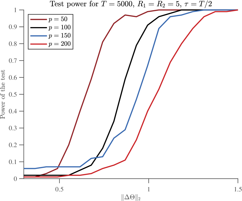
Figure 1: Test power depending on the dimension of transition matrices

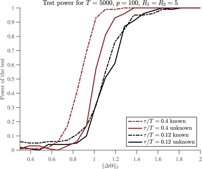
Figure 2: Test power for known or unknown location of the change-point

To calculate the test statistic $\mathcal{G}(t)$ we need to find the solutions $\widehat{\Theta}_{1}^{t}$ and $\widehat{\Theta}_{2}^{t}$ of the SDPs (11) and (12). The estimation quality of the transition matrices depends on the choice of constants in the regularization parameters $\lambda_{1}^{t}:=\tilde{c}_{1}\sqrt{p/t}$ and $\lambda_{2}^{t}:=\tilde{c}_{2}\sqrt{p/(T-t)}$. We tune the constants $\tilde{c}_{i}$ by cross-validation in the following way. We estimate the transition matrices $\Theta_{1}$ and $\Theta_{2}$ using, respectively, the first and the last $\lfloor\delta Th\rfloor$ observations $X_{1},\dots,X_{\lfloor\delta Th\rfloor}$ and $X_{T-\lfloor Th\rfloor},\dots,X_{T-\lfloor(1-\delta)Th\rfloor}$, where $\delta\in(0,1)$ is chosen a priori. Let $\widehat{\Theta}_{1,\tilde{c}_{1}}$ and $\widehat{\Theta}_{2,\tilde{c}_{2}}$ be the corresponding solutions of SDPs (11) and (12) with the regularization constants $\tilde{c}_{1}$ and $\tilde{c}_{2}$ varying within some appropriately chosen grid. The optimal constants $\tilde{c}_{1}^{*}$ and $\tilde{c}_{2}^{*}$ will minimize the least-squares criteria for $\widehat{\Theta}_{1,_{\tilde{c}_{1}}}$ and $\widehat{\Theta}_{2,\tilde{c}_{2}}$ calculated over the interval of size $(1-\delta)Th$ :

$$\tilde{c}_{1}^{*}=\mathop{\rm arg\,min}_{\tilde{c}_{1}\in\mathrm{grid}}\sum_{t=\lfloor\delta Th\rfloor}^{\lfloor Th\rfloor-1}\|X_{t+1}-\widehat{\Theta}_{1,\tilde{c}_{1}}X_{t}\|_{2}^{2},\quad\tilde{c}_{2}^{*}=\mathop{\rm arg\,min}_{\tilde{c}_{2}\in\mathrm{grid}}\sum_{t=T-\lfloor(1-\delta)Th\rfloor}^{T-1}\|X_{t+1}-\widehat{\Theta}_{2,\tilde{c}_{2}}X_{t}\|_{2}^{2}.$$

To obtain the plug-in estimates $\widehat{\Theta}_{1}^{t}$ and $\widehat{\Theta}_{2}^{t}$ used in $\mathcal{G}(t)$, we take the regularization parameters $\lambda_{1}^{t}$ and $\lambda_{2}^{t}$ with the constants $\tilde{c}_{1}^{*}$ and $\tilde{c}_{2}^{*}$. The numerical solution to the SDPs is calculated using the accelerated gradient decent algorithm of Ji and Ye, (2009).

The theoretical quantile of the change-point detection procedure depends on an unknown universal constant. In this study we use Monte-Carlo simulated quantiles $q_{\alpha,t}$. The details about the quantile simulation are provided in the Appendix.

We have performed 100 simulations of $T=5000$ observations of $\mathrm{VAR}_{p}(\Theta_{1},\Theta_{2},\Sigma_{Z})$ process with independent noise, $\Sigma_{Z}=\mathop{\rm id}\nolimits_{p}$ and transition matrices $\Theta_{1}$ and $\Theta_{2}$ of the same rank $R_{1}=R_{2}=5$. The significance level $\alpha$ is fixed to 0.05. We have chosen the intervals of size $Th=5p$ for the estimation of matrices $\Theta_{1}$ and $\Theta_{2}$ with $\delta=4/5$ for the constant calibration interval. We consider the problems of testing for a change-point at a given point $\tau\in\mathcal{D}_{T}$ and at an unknown point within the set $\mathcal{D}_{T}$. In the second case the dyadic grid defined in (18) was chosen as $\mathcal{T}$.

Fig. 2 shows the dependence of the test power on the Frobenius norm of the change in transition matrices, $\|\Delta\Theta\|_{2}$, for different values of $p$ varying from $50$ to $200$. Here we test at a given point located in the middle. We see that the power decreases if the dimension increases and the detection problem becomes harder for the matrices of larger dimension. This confirms our theoretical detection rate $C\sqrt{Rp/T}$. In Fig. 2 we compare our test’s performance for a given change-point versus an unknown change-point. In this simulation the dimension is fixed, $p=100$. The bold line corresponds to the test power within the dyadic grid for the case of unknown change-point location. We see that the adaptive test performs quite well with respect to testing at a known change-point location. We can also see the impact of the change-point location to the detection rate: the detection is harder near the boundary of $\mathcal{D}_{T}$ and easier in the middle of the interval. Additional simulation results can be found in the Appendix.

Appendix A Definitions from minimax testing theory

Let ${\mathfrak{X}}=(X_{0},\dots,X_{T})$ be observed data satisfying $\mathrm{VAR}_{p}(\Theta_{1},\Theta_{2},\Sigma_{Z})$ model (3) with the change at point $\tau$ and the transition matrices $\Theta_{1}$ and $\Theta_{2}$ before and after the change. Denote by ${\mathrm{P}}^{\tau}_{\Theta_{1},\Theta_{2}}$ the distribution of ${\mathfrak{X}}$. Let $\psi:{\mathfrak{X}}\to\{0,1\}$ be a test for the presence of a change. Define the testing errors of $\psi({\mathfrak{X}})$. The type I error is given by

$$\alpha(\psi)=\sup_{(\Theta_{1},\Theta_{2})\in\mathcal{V}_{p,0}}{\mathrm{P}}_{\Theta_{1},\Theta_{2}}\{\psi({\mathfrak{X}})=1\},$$

the type II error of testing at the given point $\tau$ is defined as

$$\beta(\psi,\mathcal{R}_{p,T}^{\tau})=\sup_{(\Theta_{1},\Theta_{2})\in\mathcal{V}_{p,\tau}(\mathcal{R}_{p,T}^{\tau})}{\mathrm{P}}^{\tau}_{\Theta_{1},\Theta_{2}}\{\psi({\mathfrak{X}})=0\},$$

and the type II error of testing at an unknown change-point $\tau\in\mathcal{D}_{T}$ is defined as

$$\beta(\psi,\mathcal{R}_{p,T})=\sup_{\tau\in\mathcal{D}_{T}}\sup_{(\Theta_{1},\Theta_{2})\in\mathcal{V}_{p,\tau}(\mathcal{R}_{p,T})}{\mathrm{P}}^{\tau}_{\Theta_{1},\Theta_{2}}\{\psi({\mathfrak{X}})=0\}.$$

Let $\alpha\in(0,1)$ be a given significance level. Denote by $\Psi_{\alpha}$ the set of all tests of level at most $\alpha$:

$$\Psi_{\alpha}=\left\{\psi:\ \alpha(\psi)\leq\alpha\right\}.$$

It is important to know what are the conditions on the jump matrix $\Delta\Theta$ and the radius $\mathcal{R}_{p,T}$ that allow to detect the change-point with a given significance level and reasonable type II error. These conditions are formulated in terms of the minimax separation rate.

Definition 1.

Let $\alpha,\beta\in(0,1)$ be given. We say that the radius $\mathcal{R}^{*}_{p,T}$ is $(\alpha,\beta)$-minimax detection boundary in problem of testing the hypothesis of no change against the alternative $\mathcal{V}_{p},\tau(\mathcal{R}_{p,\mathcal{D}_{T}})$ if

$$\mathcal{R}^{*}_{p,\mathcal{D}_{T}}=\inf_{\psi\in\Psi_{\alpha}}\mathcal{R}_{p,\mathcal{D}_{T}}(\alpha,\psi),$$

where

$$\mathcal{R}_{p,\mathcal{D}_{T}}(\alpha,\psi)=\inf\Bigl{\{}\mathcal{R}>0:\ \beta(\psi,\mathcal{R})\leq\beta\Bigr{\}}.$$

The minimax detection boundary is often written as the product $\mathcal{R}^{*}_{p,\mathcal{D}_{T}}=C\varphi_{p,\mathcal{D}_{T}}$, where $\varphi_{p,\mathcal{D}_{T}}$ is called minimax detection rate and $C$ is a constant independent of $p$ and $T$. We say that the radius $\mathcal{R}_{p,\mathcal{D}_{T}}$ satisfies the upper bound condition if there exists a constant $C^{*}>0$ and a test $\psi^{*}\in\Psi_{\alpha}$ such that $\forall C>C^{*}$ $\beta(\psi^{*},\mathcal{R}_{p,\mathcal{D}_{T}})\leq\beta$. We say that $\mathcal{R}_{p,\mathcal{D}_{T}}$ satisfies the lower bound condition if for any $0<C\leq C_{*}$ there is no test of level $\alpha$ with type II error smaller than $\beta$. Our goal is to find the minimax detection rate $\varphi_{p,\mathcal{D}_{T}}$ and two constants $C_{*}$ and $C^{*}$ such that

$$C_{*}\varphi_{p,\mathcal{D}_{T}}\leq\mathcal{R}^{*}_{p,\mathcal{D}_{T}}\leq C^{*}\varphi_{p,\mathcal{D}_{T}}.$$

Appendix B Proof of the upper bound

Denote

$${\mathcal{F}}_{1}(t)=\varphi^{t}_{1}({\mathfrak{X}},\widehat{\Theta}_{2}^{t})-\varphi^{t}_{1}({\mathfrak{X}},\widehat{\Theta}_{1}^{t})\quad\mbox{and}\quad{\mathcal{F}}_{2}(t)=\varphi^{t}_{2}({\mathfrak{X}},\widehat{\Theta}_{1}^{t})-\varphi^{t}_{2}({\mathfrak{X}},\widehat{\Theta}_{2}^{t})$$

Lemma 2 (Type I error).

Let $\alpha\in(0,1)$ be a given significance level. Assume that $T/2\geq p>\log\left(8|\mathcal{T}|/\alpha\right)$. If we solve (11)–(12) with $\lambda^{t}_{1}$ and $\lambda^{t}_{2}$ defined in (13)–(14), then the type I error of test (16) is bounded by $\alpha$.

Proof.

By the union bound, the type I error of the test $\psi_{\alpha}$ can be bounded as follows,

$$\alpha(\psi_{\alpha})=\sup_{(\Theta_{1},\Theta_{2})\in\mathcal{V}_{p}(\tau,0)}{\mathrm{P}}_{\Theta_{1},\Theta_{2}}\left(\max_{t\in\mathcal{T}}\frac{\mathcal{F}(t)}{H_{\alpha,t}}>1\right)\leq\sum_{t\in\mathcal{T}}\sup_{(\Theta_{1},\Theta_{2})\in\mathcal{V}_{p}(\tau,0)}{\mathrm{P}}_{\Theta_{1},\Theta_{2}}\Bigl{\{}\mathcal{F}(t)\geq H_{\alpha,t}\Bigr{\}}.$$

Denote by $\Theta:=\Theta_{1}=\Theta_{2}$ the transition matrix of the process under the null hypothesis. To provide an $\alpha$-level test, we need to show that the type I error of testing at each point $t\in\mathcal{T}$ is bounded by $\alpha/|\mathcal{T}|$:

$$\sup_{\Theta\in\mathcal{M}_{p}(R,\gamma)}{\mathrm{P}}_{\Theta}\Bigl{\{}\mathcal{F}(t)\geq H_{\alpha,t}\Bigr{\}}\leq\alpha/|\mathcal{T}|,$$

For any two matrices $A$ and $B$ we have

$$\sum_{i=t}^{T-1} \Bigl{(}\|X_{i+1}-AX_{i}\|_{2}^{2}-\|X_{i+1}-BX_{i}\|_{2}^{2}\Bigr{)}$$

$$=\sum_{i=t}^{T-1}\Bigl{(}\|\left(\Theta-A\right)X_{i}+Z_{i+1}\|_{2}^{2}-\|\left(\Theta-B\right)X_{i}+Z_{i+1}\|_{2}^{2}\Bigr{)}$$

$$=\sum_{i=t}^{T-1}\Bigl{(}\|(\Theta-A)X_{i}\|_{2}^{2}-\|\left(\Theta-B\right)X_{i}\|_{2}^{2}\Bigr{)}+2\sum_{i=t}^{T-1}\Bigl{(}\left\langle(\Theta-A)X_{i},Z_{i+1}\right\rangle-\left\langle(\Theta-B)X_{i},Z_{i+1}\right\rangle\Bigr{)}$$

$$=\|\left(\Theta-A\right){\mathfrak{X}}_{\geq t}\|_{2}^{2}-\|\left(\Theta-B\right){\mathfrak{X}}_{\geq t}\|_{2}^{2}+2\left\langle\left(B-A\right){\mathfrak{X}}_{\geq t},\mathfrak{Z}_{\geq t}\right\rangle.$$ (20)

A similar calculation provides

$$\sum_{i=0}^{t-1}\left(\|X_{i+1}-AX_{i}\|_{2}^{2}-\|X_{i+1}-BX_{i}\|_{2}^{2}\right)$$

$$\hskip 56.9055pt=\|\left(\Theta-A\right){\mathfrak{X}}_{<t}\|_{2}^{2}-\|\left(\Theta-B\right)X_{i}\|_{2}^{2}+2\left\langle\left(B-A\right){\mathfrak{X}}_{\geq t},\mathfrak{Z}_{\geq t}\right\rangle.$$ (21)

Since the test statistic $\mathcal{F}(t)$ depends on the location of $t$ with respect to the boundary, we will consider four following cases: (a) $t\geq T/2$ and $T-t\leq p$, $t\geq p$, (b) $t\geq T/2$ and $T-t\geq p$, (c) $t\leq T/2$ and $t\leq p$, $T-t\geq T-p$, and (d) $t\leq T/2$ and $t\geq p$.

Note that the assumption $p\leq T/2$ is important. It implies, for example, that $t\geq p$ if $T-t\leq p$ and $t\geq T/2$.

By symmetry, it is sufficient to consider the cases (a) and (b). Consider the case (a) when $t\geq T/2\geq p$ and $T-t\leq p$. Using (B) and (B) we have

$$\sum_{i=t}^{T-1}\left(\|X_{i+1}-\widehat{\Theta}_{1}^{t}X_{i}\|_{2}^{2}-\|X_{i+1}-\widehat{\Theta}_{2}^{t}X_{i}\|_{2}^{2}\right)$$

$$\hskip 28.45274pt=\|(\Theta-\widehat{\Theta}_{1}^{t}){\mathfrak{X}}_{\geq t}\|_{2}^{2}-\|(\Theta-\widehat{\Theta}_{2}^{t}){\mathfrak{X}}_{\geq t}\|_{2}^{2}+2\left\langle(\widehat{\Theta}_{2}^{t}-\widehat{\Theta}_{1}^{t}){\mathfrak{X}}_{\geq t},\mathfrak{Z}_{\geq t}\right\rangle.$$

Thus $\mathcal{F}(t)$ can be written as the sum of three terms,

$$\mathcal{F}(t) =\frac{1}{T-t}\left(\|(\Theta-\widehat{\Theta}_{1}^{t}){\mathfrak{X}}_{\geq t}\|_{2}^{2}-\|(\Theta-\widehat{\Theta}_{2}^{t}){\mathfrak{X}}_{\geq t}\|_{2}^{2}\right)+\frac{2}{T-t}\left\langle(\widehat{\Theta}_{2}^{t}-\widehat{\Theta}_{1}^{t}){\mathfrak{X}}_{\geq t},\mathfrak{Z}_{\geq t}\right\rangle.$$

$$+\lambda_{2}^{t}\left(\|\widehat{\Theta}_{1}^{t}\mathfrak{X}_{\geq t}\|_{*}-\|\Theta\mathfrak{X}_{\geq t}\|_{*}+\|\Theta\mathfrak{X}_{\geq t}\|_{*}-\|\widehat{\Theta}_{2}^{t}\mathfrak{X}_{\geq t}\|_{*}\right):=A+B+C.$$ (22)

Introduce the following random events,

$$\mathcal{A}=\left\{\|\mathfrak{Z}_{\geq t}\|_{\mathrm{op}}\leq c_{1}^{*}\sqrt{\|\Sigma_{Z}\|_{\mathrm{op}}}\left(\sqrt{T-t}+\sqrt{p}+\sqrt{\log\frac{8|\mathcal{T}|}{\alpha}}\right)\right\},$$

$$\mathcal{B}_{1}=\left\{\|\widehat{\Theta}_{1}^{t}-\Theta\|_{2}^{2}\leq c^{*}\frac{\kappa^{2}(\Sigma)}{(1-\gamma)^{2}}\frac{Rp}{t}\right\}\quad\mbox{and}\quad\mathcal{B}_{2}=\left\{\|\widehat{\Theta}_{2}^{t}-\Theta\|_{2}^{2}\leq c^{*}\frac{\kappa^{2}(\Sigma)}{(1-\gamma)^{2}}\frac{Rp}{T-t}\right\}$$

Lemma 9 implies that ${\mathrm{P}}(\mathcal{A})\geq 1-\dfrac{\alpha}{4|\mathcal{T}|}$ and Proposition 5 gives ${\mathrm{P}}(\mathcal{B}_{i})\geq 1-c_{2}\exp(-c_{3}p)\geq 1-\dfrac{\alpha}{4|\mathcal{T}|}$ for sufficiently large $p$. Thus, we have

$${\mathrm{P}}_{\Theta}\{\mathcal{F}(t)>H_{\alpha,t}\}\leq{\mathrm{P}}_{\Theta}\Bigl{\{}\{\mathcal{F}(t)>H_{\alpha,t}\}\cap\{\mathcal{A}\cap\mathcal{B}_{1}\cap\mathcal{B}_{2}\}\Bigr{\}}+{\mathrm{P}}(\mathcal{A}^{c})+{\mathrm{P}}_{\Theta}(\mathcal{B}_{1}^{c})+{\mathrm{P}}_{\Theta}(\mathcal{B}_{2}^{c}).$$

To show that the type I error is bounded by $\alpha$, we have to show that the first probability is bounded by $\alpha/(4|\mathcal{T}|)$.

Consider first the scalar product term $B$ in (22). We have

$$\left(\widehat{\Theta}_{2}^{t}-\widehat{\Theta}_{1}^{t}\right)\mathfrak{X}_{\geq t} =\left(\Theta-\widehat{\Theta}_{1}^{t}\right)\mathfrak{X}_{\geq t}+\left(\widehat{\Theta}_{2}^{t}-\Theta\right)\mathfrak{X}_{\geq t}$$

$$=\left(\Theta-\widehat{\Theta}_{1}^{t}\right)\mathfrak{X}_{\geq t}-\mathbf{Pr}_{\Theta\mathfrak{X}_{\geq t}}\Bigl{[}\Theta\mathfrak{X}_{\geq t}\Bigr{]}+\mathbf{Pr}_{\Theta\mathfrak{X}_{\geq t}}\Bigl{[}\widehat{\Theta}_{2}^{t}\mathfrak{X}_{\geq t}\Bigr{]}+\mathbf{Pr}^{\bot}_{\Theta\mathfrak{X}_{t}}\Bigl{[}\widehat{\Theta}_{2}^{t}\mathfrak{X}_{\geq t}\Bigr{]}.$$

Using this identity and the Hölder inequality, we obtain

$$\left\langle\left(\widehat{\Theta}_{2}^{t}-\widehat{\Theta}_{1}^{t}\right)\mathfrak{X}_{\geq t},\mathfrak{Z}_{\geq t}\right\rangle \leq\|\left(\widehat{\Theta}_{1}^{t}-\Theta\right)\mathfrak{X}_{\geq t}\|_{*}\|\mathfrak{Z}_{\geq t}\|_{\mathrm{op}}$$

$$+\|\mathbf{Pr}_{\Theta\mathfrak{X}_{\geq t}}\left[\left(\Theta-\widehat{\Theta}_{2}^{t}\right)\mathfrak{X}_{\geq t}\right]\|_{*}\|\mathfrak{Z}_{\geq t}\|_{\mathrm{op}}+\|\mathbf{Pr}^{\bot}_{\Theta\mathfrak{X}_{\geq t}}\left[\widehat{\Theta}_{2}^{t}\mathfrak{X}_{\geq t}\right]\|_{*}\|\mathfrak{Z}_{\geq t}\|_{\mathrm{op}}.$$

By Lemma 9, taking into account the fact that $p\geq T-t$ and $p>\log(8|\mathcal{T}|/\alpha)$, we obtain that with probability at least $1-\alpha/(4|\mathcal{T}|)$,

$$\frac{2}{T-t}\|\mathfrak{Z}_{\geq t}\|_{\mathrm{op}}\leq 6c_{1}^{*}\sqrt{\|\Sigma_{Z}\|_{\mathrm{op}}}\frac{\sqrt{p}}{T-t}=\lambda_{2}^{t}.$$

Thus, given $\mathcal{A}$, we have

$$B\leq\lambda^{t}_{2}\|(\widehat{\Theta}_{1}^{t}-\Theta)\mathfrak{X}_{\geq t}\|_{*}+\lambda^{t}_{2}\|\mathbf{Pr}_{\Theta\mathfrak{X}_{\geq t}}\left[(\Theta-\widehat{\Theta}_{2}^{t})\mathfrak{X}_{\geq t}\right]\|_{*}+\|\mathbf{Pr}^{\bot}_{\Theta\mathfrak{X}_{\geq t}}\left[\widehat{\Theta}_{2}^{t}\mathfrak{X}_{\geq t}\right]\|_{*}$$

Using the triangle inequality, $\|\widehat{\Theta}_{1}^{t}\mathfrak{X}_{\geq t}\|_{*}-\|\Theta\mathfrak{X}_{\geq t}\|_{*}\leq\|\left(\widehat{\Theta}_{1}^{t}-\Theta\right)\mathfrak{X}_{\geq t}\|_{*}$ and the fact that by (41), $\|\Theta\mathfrak{X}_{\geq t}\|_{*}-\|\widehat{\Theta}_{2}^{t}\mathfrak{X}_{\geq t}\|_{*}\leq\|\mathbf{Pr}_{\Theta\mathfrak{X}_{\geq t}}\left[\left(\Theta-\widehat{\Theta}_{2}^{t}\right)\mathfrak{X}_{\geq t}\right]\|_{*}-\|\mathbf{Pr}^{\bot}_{\Theta\mathfrak{X}_{\geq t}}\left[\left(\Theta-\widehat{\Theta}_{2}^{t}\right)\mathfrak{X}_{\geq t}\right]\|_{*}$, we obtain for the term $C$,

$$C\leq\lambda^{t}_{2}\|\left(\widehat{\Theta}_{1}^{t}-\Theta\right)\mathfrak{X}_{\geq t}\|_{*}+\lambda^{t}_{2}\|\mathbf{Pr}_{\Theta\mathfrak{X}_{\geq t}}\left[\left(\Theta-\widehat{\Theta}_{2}^{t}\right)\mathfrak{X}_{\geq t}\right]\|_{*}-\lambda^{t}_{2}\|\mathbf{Pr}^{\bot}_{\Theta\mathfrak{X}_{\geq t}}\left[\widehat{\Theta}_{2}^{t}\mathfrak{X}_{\geq t}\right]\|_{*}.$$

Gathering these bounds, we obtain that given $\mathcal{A}$,

$$\mathcal{F}(t) \leq\frac{1}{T-t}\|\left(\Theta-\widehat{\Theta}_{1}^{t}\right)\mathfrak{X}_{\geq t}\|_{2}^{2}-\frac{1}{T-t}\|\left(\Theta-\widehat{\Theta}_{2}^{t}\right)\mathfrak{X}_{\geq t}\|_{2}^{2}$$

$$+2\lambda^{t}_{2}\|\left(\widehat{\Theta}_{1}^{t}-\Theta\right)\mathfrak{X}_{\geq t}\|_{*}+2\lambda^{t}_{2}\|\mathbf{Pr}_{\Theta\mathfrak{X}_{\geq t}}\left[\left(\Theta-\widehat{\Theta}_{2}^{t}\right)\mathfrak{X}_{\geq t}\right]\|_{*}.$$ (23)

Using Lemma 7, we get the bound

$$\|\widehat{\Theta}_{1}^{t}-\Theta\|_{*}\leq\|\mathbf{Pr}^{\bot}_{\Theta}\left[\widehat{\Theta}_{1}^{t}-\Theta\right]\|_{*}+\|\mathbf{Pr}_{\Theta}\left[\widehat{\Theta}_{1}^{t}-\Theta\right]\|_{*}\leq 6\|\mathbf{Pr}_{\Theta}\left[\widehat{\Theta}_{1}^{t}-\Theta\right]\|_{*}.$$

Taking into account that ${\rm rank}\left(\mathbf{Pr}_{\Theta}\Bigl{[}\widehat{\Theta}_{1}^{t}-\Theta\Bigr{]}\right)\leq 2{\rm rank}(\Theta)=2R$, using $\|A\|_{*}^{2}\leq{\rm rank}(A)\|A\|_{2}^{2}$ and the trivial inequality $2ab\leq a^{2}+b^{2}$, we get

$$2\lambda^{t}_{2}\|\left(\widehat{\Theta}_{1}^{t}-\Theta\right)\mathfrak{X}_{\geq t}\|_{*} \leq 2\lambda^{t}_{2}\|\widehat{\Theta}_{1}^{t}-\Theta\|_{*}\|\mathfrak{X}_{\geq t}\|_{\mathrm{op}}$$

$$\leq 12\lambda^{t}_{2}\|\mathbf{Pr}_{\Theta}\left[\widehat{\Theta}_{1}^{t}-\Theta\right]\|_{*}\|\mathfrak{X}_{\geq t}\|_{\mathrm{op}}$$

$$\leq 12\lambda^{t}_{2}\sqrt{2R}\|\widehat{\Theta}_{1}^{t}-\Theta\|_{2}\|\mathfrak{X}_{\geq t}\|_{\mathrm{op}}$$

$$\leq 2\left(\lambda^{t}_{2}\right)^{2}R(T-t)+\dfrac{36}{T-t}\|\widehat{\Theta}_{1}^{t}-\Theta\|_{2}^{2}\|\mathfrak{X}_{\geq t}\|_{\mathrm{op}}^{2}.$$

Thus by Proposition 5, given $\mathcal{B}_{1}$ with probability at least $1-c_{2}\exp(-c_{3}p)\geq 1-\alpha/(4|\mathcal{T}|)$, we have

$2\lambda^{t}_{2}\|\left(\widehat{\Theta}_{1}^{t}-\Theta\right)\mathfrak{X}_{\geq t}\|_{*}\leq 2\left(\lambda^{t}_{2}\right)^{2}R(T-t)+\dfrac{36c^{*}Rp}{t(T-t)}\dfrac{\kappa^{2}(\Sigma)}{(1-\gamma)^{2}}\|\mathfrak{X}_{\geq t}\|_{\mathrm{op}}^{2}$

Since ${\rm rank}\left(\Theta\mathfrak{X}_{t}\right)\leq{\rm rank}(\Theta)$, we have, using the same argument as above, we have

$$2\lambda^{t}_{2}\|\mathbf{Pr}_{\Theta\mathfrak{X}_{\geq t}}\left[(\Theta-\widehat{\Theta}_{2}^{t})\mathfrak{X}_{\geq t}\right]\|_{*} \leq 2\lambda^{t}_{2}\sqrt{2R}\|(\Theta-\widehat{\Theta}_{2}^{t})\mathfrak{X}_{\geq t}\|_{2}$$

$$\leq 2\left(\lambda^{t}_{2}\right)^{2}R(T-t)+\frac{1}{T-t}\|(\Theta-\widehat{\Theta}_{2}^{t})\mathfrak{X}_{\geq t}\|_{2}^{2}.$$

Similarly, by Proposition 5, given $\mathcal{B}_{2}$ we have

$$\frac{1}{T-t}\|(\Theta-\widehat{\Theta}_{1}^{t})\mathfrak{X}_{\geq t}\|_{2}^{2}\leq\dfrac{c^{*}Rp}{t(T-t)}\dfrac{\kappa^{2}(\Sigma)}{(1-\gamma)^{2}}\|\mathfrak{X}_{\geq t}\|_{\mathrm{op}}^{2}$$

Finally, for sufficiently large $p$, with the probability at least $1-\alpha/(4|\mathcal{T}|)$, (23) and the above inequalities and the definition of $\lambda_{2}^{t}$ imply, given the event $\mathcal{A}\cap\mathcal{B}_{1}\cap\mathcal{B}_{2}$,

$$\mathcal{F}(t)\leq\dfrac{37c^{*}Rp}{t(T-t)}\dfrac{\kappa^{2}(\Sigma)}{(1-\gamma)^{2}}\|\mathfrak{X}_{\geq t}\|_{\mathrm{op}}^{2}+\dfrac{144(c_{1}^{*})^{2}\|\Sigma_{Z}\|_{\mathrm{op}}Rp}{T-t}.$$

Thus, for any $\Theta\in\mathcal{M}_{p}(R,\gamma)$,

$${\mathrm{P}}_{\Theta}\Bigl{\{}\{\mathcal{F}(t)>H_{\alpha,t}\} \cap\{\mathcal{A}\cap\mathcal{B}_{1}\cap\mathcal{B}_{2}\}\Bigr{\}}$$

$$\leq{\mathrm{P}}\left\{\dfrac{37c^{*}Rp}{t(T-t)}\dfrac{\kappa^{2}(\Sigma)}{(1-\gamma)^{2}}\|\mathfrak{X}_{\geq t}\|_{\mathrm{op}}^{2}+\dfrac{144(c^{*})^{2}Rp\|\Sigma_{Z}\|_{\mathrm{op}}}{T-t}>H_{\alpha,t}\right\}$$

$$\leq{\mathrm{P}}\left\{\frac{1}{T-t}\|\mathfrak{X}_{\geq t}\|_{\mathrm{op}}^{2}\geq 2\|\Sigma\|_{\mathrm{op}}\Bigl{(}1+\frac{c_{0}}{1-\gamma}\frac{p+\log(8|\mathcal{T}|/\alpha)}{T-t}\Bigr{)}\right\}\leq\frac{\alpha}{4|\mathcal{T}|},$$

where we used Lemma 8 with $\delta=\dfrac{\alpha}{8|\mathcal{T}|}$, $T-t\leq p$, $t\geq p$ and the fact that for a sufficiently large universal constant $C$ depending on $c^{*}$, $c_{0}$ and $c_{1}^{*}$, we have the bound

$$H_{\alpha,t} =C\max\Bigl{(}\|\Sigma_{Z}\|_{\mathrm{op}},\dfrac{\kappa^{2}(\Sigma)}{(1-\gamma)^{2}}\|\Sigma\|_{\mathrm{op}}\Bigr{)}\dfrac{Rp}{Tq^{2}(t/T)}\left(1+\frac{1}{1-\gamma}\dfrac{p+\log(8|\mathcal{T}|/\alpha)}{T}\right)$$

$$\geq\dfrac{144(c_{1}^{*})^{2}Rp\|\Sigma_{Z}\|_{\mathrm{op}}}{T-t}+\frac{74c^{*}Rp}{t}\dfrac{\kappa^{2}(\Sigma)}{(1-\gamma)^{2}}\|\Sigma\|_{\mathrm{op}}\Bigl{(}1+\frac{c_{0}}{1-\gamma}\frac{p+\log(8|\mathcal{T}|/\alpha)}{T-t}\Bigr{)}.$$

Let us turn to the case (b) of the candidate change-point located far from the endpoints of the interval, $T-t\geq p$ and $t\geq T/2$. Calculations similar to the case (a) imply

$$\mathcal{F}(t) =\frac{1}{T-t}\sum_{i=t}^{T-1}\left(\|\left(\Theta-\widehat{\Theta}_{1}^{t}\right)X_{i}\|_{2}^{2}-\|\left(\Theta-\widehat{\Theta}_{2}^{t}\right)X_{i}\|_{2}^{2}\right)+\frac{2}{T-t}\left\langle\left(\widehat{\Theta}_{2}^{t}-\widehat{\Theta}_{1}^{t}\right),\mathfrak{Z}_{\geq t}\mathfrak{X}^{{\mathrm{\scriptscriptstyle T}}}_{\geq t}\right\rangle$$

$$+\lambda_{2}^{t}\left(\|\widehat{\Theta}_{1}^{t}\|_{*}-\|\Theta\|_{*}+\|\Theta\|_{*}-\|\left(\widehat{\Theta}_{2}^{t}\right)\|_{*}\right)=A+B+C.$$

Introduce the random events

$$\mathcal{A}^{\prime}=\left\{\frac{1}{T-t}\|\mathfrak{Z}_{\geq t}\mathfrak{X}_{\geq t}^{{\mathrm{\scriptscriptstyle T}}}\|_{\mathrm{op}}\leq\frac{c_{2}^{*}\|\Sigma\|_{\mathrm{op}}}{1-\gamma}\sqrt{\frac{p}{T-t}}\right\}\quad\mbox{and}\quad\mathcal{D}=\left\{\frac{1}{T-t}\sigma_{\min}({\mathfrak{X}}_{\geq t}^{\mathrm{\scriptscriptstyle T}}{\mathfrak{X}}_{\geq t})\geq\frac{\sigma_{\min}(\Sigma_{2})}{4}\right\}.$$

Lemma 10 and Lemma 8 imply that ${\mathrm{P}}(\mathcal{A}^{\prime})\geq 1-\alpha/(8|\mathcal{T}|)$ and ${\mathrm{P}}(\mathcal{D}^{\prime})\geq 1-\alpha/(8|\mathcal{T}|)$ for sufficiently large such that$p\geq a_{1}\log(8|\mathcal{T}|/a_{2})$ for some universal constants $a_{1},a_{2}>0$. Similarly to the case (a), we have

$${\mathrm{P}}_{\Theta}\{\mathcal{F}(t)>H_{\alpha,t}\}\leq{\mathrm{P}}_{\Theta}\Bigl{\{}\{\mathcal{F}(t)>H_{\alpha,t}\}\cap\mathcal{A}^{\prime}\cap\mathcal{B}_{1}\cap\mathcal{B}_{2}\cap\mathcal{D}\Bigr{\}}+{\mathrm{P}}_{\Theta}((\mathcal{A}^{\prime})^{c})+{\mathrm{P}}_{\Theta}(\mathcal{B}_{1}^{c})+{\mathrm{P}}_{\Theta}(\mathcal{B}_{2}^{c})+{\mathrm{P}}_{\Theta}(\mathcal{D}^{c}).$$

We have to show that the first probability is bounded by $\alpha/(4|\mathcal{T}|)$. As in the previous case, we get using the Hölder inequality,

$$\left\langle\left(\widehat{\Theta}_{2}^{t}-\widehat{\Theta}_{1}^{t}\right),\mathfrak{Z}_{\geq t}\mathfrak{X}^{{\mathrm{\scriptscriptstyle T}}}_{\geq t}\right\rangle \leq\|\widehat{\Theta}_{1}^{t}-\Theta\|_{*}\|\mathfrak{Z}_{\geq t}\mathfrak{X}^{{\mathrm{\scriptscriptstyle T}}}_{\geq t}\|_{\mathrm{op}}$$

$$+\|\mathbf{Pr}_{\Theta}\left(\Theta-\widehat{\Theta}_{2}^{t}\right)\|_{*}\|\mathfrak{Z}_{\geq t}\mathfrak{X}^{{\mathrm{\scriptscriptstyle T}}}_{\geq t}\|_{\mathrm{op}}+\|\mathbf{Pr}^{\bot}_{\Theta}\left(\widehat{\Theta}_{2}^{t}\right)\|_{*}\|\mathfrak{Z}_{\geq t}\mathfrak{X}^{{\mathrm{\scriptscriptstyle T}}}_{\geq t}\|_{\mathrm{op}}.$$

Remind that $\lambda^{t}_{2}=\dfrac{2c_{2}^{*}\|\Sigma\|_{\mathrm{op}}}{1-\gamma}\sqrt{\displaystyle{\frac{p}{T-t}}}$. Lemma 10 implies that for sufficiently large $p$, with the probability at least $1-k_{1}\exp(-k_{2}p)$,

$$\dfrac{2}{T-t}\|\mathfrak{Z}_{\geq t}\mathfrak{X}^{{\mathrm{\scriptscriptstyle T}}}_{\geq t}\|_{\mathrm{op}}\leq\dfrac{2c_{2}^{*}\|\Sigma\|_{\mathrm{op}}}{1-\gamma}\sqrt{\dfrac{p}{T-t}}=\lambda_{2}^{t}.$$

Thus, given the event $\mathcal{A}^{\prime}$, we get $B\leq\lambda^{t}_{2}\|\widehat{\Theta}_{1}^{t}-\Theta\|_{*}+\lambda^{t}_{2}\|\mathbf{Pr}_{\Theta}\left[\Theta-\widehat{\Theta}_{2}^{t}\right]\|_{*}+\lambda^{t}_{2}\|\mathbf{Pr}^{\bot}_{\Theta}\left[\widehat{\Theta}_{2}^{t}\right]\|_{*}$. Similarly, for the term $C$, using the triangle inequality and the inequality (41) implying that $\|\Theta\|_{*}-\|\widehat{\Theta}_{2}^{t}\|_{*}\leq\|\mathbf{Pr}_{\Theta}\left[\Theta-\widehat{\Theta}_{2}^{t}\right]\|_{*}-\|\mathbf{Pr}^{\bot}_{\Theta}\left[\Theta-\widehat{\Theta}_{2}^{t}\right]\|_{*}$, we obtain

$$C\leq\lambda^{t}_{2}\|\widehat{\Theta}_{1}^{t}-\Theta\|_{*}+\lambda^{t}_{2}\|\mathbf{Pr}_{\Theta}\left[\Theta-\widehat{\Theta}_{2}^{t}\right]\|_{*}-\lambda^{t}_{2}\|\mathbf{Pr}^{\bot}_{\Theta}\left[\widehat{\Theta}_{2}^{t}\right]\|_{*}.$$

Thus, given $\mathcal{A}^{\prime}$, we have

$$\mathcal{F}(t)\leq\dfrac{1}{T-t}\|\left(\Theta-\widehat{\Theta}_{1}^{t}\right)\mathfrak{X}_{\geq t}\|_{2}^{2}-\dfrac{1}{T-t}\|\left(\Theta-\widehat{\Theta}_{2}^{t}\right)\mathfrak{X}_{\geq t}\|_{2}^{2}+2\lambda^{t}_{2}\|\widehat{\Theta}_{1}^{t}-\Theta\|_{*}+2\lambda^{t}_{2}\|\mathbf{Pr}_{\Theta}\left(\Theta-\widehat{\Theta}_{2}^{t}\right)\|_{*}.$$

As in the case (a), using Lemma 7 and $2ab\leq a^{2}+b^{2}$, we can bound the last two terms of this inequality

$$2\lambda^{t}_{2}\|\widehat{\Theta}_{1}^{t}-\Theta\|_{*}\leq 12\lambda^{t}_{2}\sqrt{2R}\|\widehat{\Theta}_{1}^{t}-\Theta\|_{2}\leq\dfrac{9R\left(\lambda^{t}_{2}\right)^{2}}{\sigma_{\min}(\Sigma)}+8\sigma_{\max}(\Sigma)\|\Theta-\widehat{\Theta}_{1}^{t}\|_{2}^{2}$$

and

$$2\lambda^{t}_{2}\|\mathbf{Pr}_{\Theta}\left(\Theta-\widehat{\Theta}_{2}^{t}\right)\|_{*}\leq 2\lambda^{t}_{2}\sqrt{2R}\|\widehat{\Theta}_{2}^{t}-\Theta\|_{2}\\ \leq\dfrac{8R\left(\lambda^{t}_{2}\right)^{2}}{\sigma_{\min}(\Sigma)}+\dfrac{\sigma_{\min}(\Sigma)}{4}\|\widehat{\Theta}_{2}^{t}-\Theta\|_{2}^{2}.$$

By Proposition 5, with probability at least $1-\alpha/(4|\mathcal{T}|)$,

$$\frac{1}{T-t}\|\left(\Theta-\widehat{\Theta}_{1}^{t}\right)\mathfrak{X}_{\geq t}\|_{2}^{2}\leq\dfrac{c^{*}Rp}{t(T-t)}\dfrac{\kappa^{2}(\Sigma)}{(1-\gamma)^{2}}\|\mathfrak{X}_{\geq t}\|_{\mathrm{op}}^{2}.$$

This implies that given $\mathcal{A}^{\prime}\cap\mathcal{B}_{1}$

$$\mathcal{F}(t) \leq\dfrac{c^{*}Rp}{t(T-t)}\dfrac{\kappa^{2}(\Sigma)}{(1-\gamma)^{2}}\|\mathfrak{X}_{\geq t}\|_{\mathrm{op}}^{2}-\dfrac{1}{T-t}\sigma_{\min}(\mathfrak{X}_{\geq t}^{{\mathrm{\scriptscriptstyle T}}}\mathfrak{X}_{\geq t})\|\Theta-\widehat{\Theta}_{2}^{t}\|_{2}^{2}+\dfrac{17R\left(\lambda^{t}_{2}\right)^{2}}{\sigma_{\min}(\Sigma)}$$

$$+8\sigma_{\max}(\Sigma)\|\Theta-\widehat{\Theta}_{1}^{t}\|_{2}^{2}+\dfrac{\sigma_{\min}(\Sigma)}{4}\|\widehat{\Theta}_{2}^{t}-\Theta\|_{2}^{2}.$$

Using the definition of $\lambda_{2}^{t}$, Lemma 8 and Proposition 5, we finally obtain that given $\mathcal{A}^{\prime}\cap\mathcal{B}_{1}\cap\mathcal{B}_{2}\cap\mathcal{D}$

$$\mathcal{F}(t) \leq\dfrac{c^{*}Rp}{t(T-t)}\dfrac{\kappa^{2}(\Sigma)}{(1-\gamma)^{2}}\|\mathfrak{X}_{\geq t}\|_{\mathrm{op}}^{2}+\dfrac{68(c_{2}^{*})^{2}\|\Sigma\|_{\mathrm{op}}^{2}}{(1-\gamma)^{2}\sigma_{\min}(\Sigma)}\frac{Rp}{T-t}+8c^{*}\sigma_{\max}(\Sigma)\frac{\kappa^{2}(\Sigma)}{(1-\gamma)^{2}}\frac{Rp}{t}$$

$$\leq\dfrac{c^{*}Rp}{t(T-t)}\dfrac{\kappa^{2}(\Sigma)}{(1-\gamma)^{2}}\|\mathfrak{X}_{\geq t}\|_{\mathrm{op}}^{2}+\max(c^{*},68(c_{2}^{*})^{2})\frac{\kappa^{2}(\Sigma)\|\Sigma\|_{{\mathrm{op}}}}{(1-\gamma)^{2}}\frac{Rp}{Tq^{2}(t/T)}$$

$$\leq C\frac{Rp}{Tq^{2}(t/T)}\dfrac{\kappa^{2}(\Sigma)}{(1-\gamma)^{2}}\left(\frac{1}{T}\|\mathfrak{X}_{\geq t}\|_{\mathrm{op}}^{2}+\|\Sigma\|_{{\mathrm{op}}}\right),$$

where $C$ is an absolute constant depending on $c^{*}$ and $c_{2}^{*}$. Note that since $T-t>p$ and $T-t\leq T/2$, we have the following bound for a sufficiently large universal constant $C$,

$$H_{\alpha,t} \geq C\dfrac{\kappa^{2}(\Sigma)\|\Sigma\|_{\mathrm{op}}}{(1-\gamma)^{2}}\dfrac{Rp}{Tq^{2}(t/T)}\left(1+\frac{T-t}{T}\left(1+\frac{c_{0}}{1-\gamma}\left(1+\dfrac{\log(8|\mathcal{T}|/\alpha)}{T-t}\right)\right)\right).$$

Using this fact and Lemma 8 with $\delta=\dfrac{\alpha}{8|\mathcal{T}|}$, we obtain that for any $\Theta\in\mathcal{M}_{p}(R,\gamma)$,

$${\mathrm{P}}_{\Theta}\Bigl{\{}\{\mathcal{F}(t)>H_{\alpha,t}\} \cap\{\mathcal{A}^{\prime}\cap\mathcal{B}_{1}\cap\mathcal{B}_{2}\}\Bigr{\}}\leq{\mathrm{P}}\left\{C\frac{Rp}{Tq^{2}(t/T)}\dfrac{\kappa^{2}(\Sigma)}{(1-\gamma)^{2}}\left(\frac{1}{T}\|\mathfrak{X}_{\geq t}\|_{\mathrm{op}}^{2}+\|\Sigma\|_{{\mathrm{op}}}\right)>H_{\alpha,t}\right\}$$

$$\leq{\mathrm{P}}\left\{\frac{1}{T-t}\|\mathfrak{X}_{\geq t}\|_{\mathrm{op}}^{2}\geq 2\|\Sigma\|_{\mathrm{op}}\left(1+\frac{c_{0}}{1-\gamma}\left(1+\frac{\log(8|\mathcal{T}|/\alpha)}{T-t}\right)\right)\right\}\leq\frac{\alpha}{4|\mathcal{T}|}$$

and the lemma follows. ∎

Lemma 3 (Type II error).

Let $\beta\in(0,1)$ be given significance level such that $p>\max\Bigl{(}k_{2}^{-1}\log(4k_{1}/\beta)\Bigr{)},\\ c_{3}^{-1}\log(4c_{2}/\beta),\log(8/\beta)\Bigr{)}$, where $k_{1},k_{2},c_{2},c_{3}$ are the constants from Proposition 5 and Lemma 10. Assume that

$$q^{2}\Bigl{(}\frac{\tau}{T}\Bigr{)}\|\Theta_{1}-\Theta_{2}\|_{2}^{2}\geq\Xi(\Sigma_{1},\Sigma_{2},\Sigma,\gamma)\frac{Rp}{T}\left(1+\frac{\log(8|\mathcal{T}|/\alpha)+\log(8/\beta)}{T}\right),$$ (24)

where, for some absolute constant $C^{*}$,

$$\Xi(\Sigma_{1},\Sigma_{2},\Sigma,\gamma)=\frac{C^{*}}{(1-\gamma)^{3}}\frac{\mathfrak{M}_{1}\vee\mathfrak{M}_{2}}{\mathfrak{m}}$$

with

$$\mathfrak{M}_{1} =\max\Bigl{(}\frac{\|\Sigma_{2}\|_{{\mathrm{op}}}^{2}}{\sigma_{\min}(\Sigma_{Z})\wedge\sigma_{\min}(\Sigma_{1})},\frac{\|\Sigma_{1}\|_{{\mathrm{op}}}^{2}}{\sigma_{\min}(\Sigma_{Z})\wedge\sigma_{\min}(\Sigma_{2})}\Bigr{)}$$ (25)

$$\mathfrak{M}_{2} =\max\Bigl{(}\kappa^{2}(\Sigma_{1})\|\Sigma_{2}\|_{{\mathrm{op}}},\kappa^{2}(\Sigma_{2})\|\Sigma_{1}\|_{{\mathrm{op}}},\kappa^{2}(\Sigma)\|\Sigma\|_{\mathrm{op}},\|\Sigma_{Z}\|_{\mathrm{op}}\Bigr{)}$$ (26)

and

$$\mathfrak{m}=\sigma_{\min}(\Sigma_{Z})\wedge\sigma_{\min}(\Sigma_{1})\wedge\sigma_{\min}(\Sigma_{2}).$$ (27)

Then, if we solve (11)–(12) with $\lambda^{t}_{1}$ and $\lambda^{t}_{2}$ given by (13) and (14), the type II error of the test $\psi_{\alpha}$ defined by (16) is bounded by $\beta$.

Proof.

We consider the case of $\mathcal{T}=\mathcal{D}_{T}$. Let $\tau\in\mathcal{D}_{T}$ be the true change-point. The type II error of the test $\psi_{\alpha}$ is defined as

$$\beta(\psi_{\alpha},\mathcal{R}_{\rho,\mathcal{D}_{T}}) =\sup_{\tau\in\mathcal{D}_{T}}\sup_{(\Theta_{1},\Theta_{2})\in V_{p}(\tau,\mathcal{R}_{p,\mathcal{D}_{T}})}{\mathrm{P}}_{\Theta_{1},\Theta_{2}}^{\tau}\Bigl{\{}\psi_{\alpha}=0\Bigr{\}}$$

$$=\sup_{\tau\in\mathcal{D}_{T}}\sup_{(\Theta_{1},\Theta_{2})\in V_{p}(\tau,\mathcal{R}_{p,\mathcal{D}_{T}})}{\mathrm{P}}_{\Theta_{1},\Theta_{2}}^{\tau}\Bigr{\{}\max_{t\in\mathcal{T}}\frac{\mathcal{F}(t)}{H_{\alpha,t}}<1\Bigr{\}}$$

$$\leq\inf_{t\in\mathcal{T}}\sup_{\tau\in\mathcal{D}_{T}}\sup_{(\Theta_{1},\Theta_{2})\in V_{p}(\tau,\mathcal{R}_{p,\mathcal{D}_{T}})}{\mathrm{P}}_{\Theta_{1},\Theta_{2}}^{\tau}\Bigr{\{}\mathcal{F}(t)<H_{\alpha,t}\Bigr{\}}$$

$$\leq\sup_{\tau\in\mathcal{D}_{T}}\sup_{(\Theta_{1},\Theta_{2})\in V_{p}(\tau,\mathcal{R}_{p,\mathcal{D}_{T}})}{\mathrm{P}}_{\Theta_{1},\Theta_{2}}^{\tau}\Bigr{\{}\mathcal{F}(\tau)<H_{\alpha,\tau}\Bigr{\}}.$$

We have to show that if the minimal jump energy satisfies condition (24), then the type II error of the test is at most $\beta$, ${\mathrm{P}}_{\Theta_{1},\Theta_{2}}^{\tau}\Bigr{\{}\mathcal{F}(\tau)<H_{\alpha,\tau}\Bigr{\}}\leq\beta$. As in the case of the type I error, we have to consider four cases of location of the change-point $\tau$ with respect to $T/2$ and the boundaries.

Consider the case (a) of $\tau\geq T/2$ and $T-\tau\leq p$. Let us introduce the events

$$\mathcal{A}=\left\{\|\mathfrak{Z}_{\geq t}\|_{\mathrm{op}}\leq c_{1}^{*}\sqrt{\|\Sigma_{Z}\|_{\mathrm{op}}}\left(\sqrt{T-\tau}+\sqrt{p}+\sqrt{\log\frac{8}{\beta}}\right)\right\},\quad\mathcal{B}_{1}=\left\{\|\widehat{\Theta}_{1}^{t}-\Theta_{1}\|_{2}^{2}\leq c^{*}\frac{\kappa^{2}(\Sigma_{1})}{(1-\gamma)^{2}}\frac{Rp}{t}\right\},$$

$$\mathcal{C}=\left\{\frac{1}{T-\tau}\|(\Theta_{1}-\Theta_{2}){\mathfrak{X}}_{\geq\tau}\|_{2}^{2}\geq\frac{\sigma_{\min}(\Sigma_{Z})\vee\sigma_{\min}(\Sigma_{2})}{2(\gamma^{2}+1)}\|\Theta_{1}-\Theta_{2}\|_{2}^{2}\right\}.$$

Lemma 9 implies that ${\mathrm{P}}(\mathcal{A})\geq 1-\beta/4$. Proposition 5 implies ${\mathrm{P}}(\mathcal{B}_{1})\geq 1-c_{2}\exp(-c_{3}p)\geq 1-\beta/4$ for sufficiently large $p$. Moreover, Lemma 11 implies that ${\mathrm{P}}(\mathcal{C})\geq 1-\beta/4$ under the condition

$$\|\Theta_{2}-\Theta_{1}\|_{2}>\frac{4\gamma(1+\gamma^{2})\sigma_{\max}(\Sigma_{2})}{\sigma_{\min}(\Sigma_{Z})\wedge\sigma_{\min}(\Sigma_{2})}\sqrt{\frac{1}{c}\frac{\log(8/\beta)}{T-\tau}}.$$ (28)

Note that (28) always holds under condition (24). We can write

$${\mathrm{P}}_{\Theta_{1},\Theta_{2}}^{\tau}\Bigr{\{}\mathcal{F}(\tau)<H_{\alpha,\tau}\Bigr{\}}\leq{\mathrm{P}}\Bigl{\{}\{\mathcal{F}(\tau)<H_{\alpha,\tau}\}\cap\mathcal{A}\cap\mathcal{B}_{1}\cap\mathcal{C}\}+{\mathrm{P}}(\mathcal{A}^{c})+{\mathrm{P}}(\mathcal{B}_{1}^{c})+{\mathrm{P}}(\mathcal{C}^{c}).$$

To bound the type II error by $\beta$, we need to show that the first probability is bounded by $\beta/4$.

By definition of $\widehat{\Theta}_{2}^{\tau}$, the test statistic can be bounded by

$$\mathcal{F}(\tau)=\varphi^{\tau}_{2}(\mathfrak{X},\widehat{\Theta}_{1}^{\tau})-\varphi^{\tau}_{2}(\mathfrak{X},\widehat{\Theta}_{2}^{\tau})\geq\varphi^{\tau}_{2}(\mathfrak{X},\widehat{\Theta}_{1}^{\tau})-\varphi^{\tau}_{2}(\mathfrak{X},\Theta_{2})$$

Taking into account that $\varphi^{\tau}_{2}(\mathfrak{X},\Theta_{2})=\dfrac{1}{T-\tau}\sum\limits_{i=\tau}^{T-1}\|Z_{i}\|_{2}^{2}+\lambda^{\tau}_{2}\|\Theta_{2}{\mathfrak{X}}_{\geq\tau}\|_{*}$ and

$$\varphi^{\tau}_{2}(\mathfrak{X},\widehat{\Theta}_{1}^{\tau}) =\dfrac{1}{T-\tau}\sum\limits_{i=\tau}^{T-1}\|\left(\Theta_{2}-\widehat{\Theta}_{1}^{\tau}\right)X_{i}\|_{2}^{2}+\dfrac{1}{T-\tau}\sum\limits_{i=\tau}^{T-1}\|Z_{i}\|_{2}^{2}$$

$$+\dfrac{2}{T-t}\left\langle\left(\Theta_{2}-\widehat{\Theta}_{1}^{\tau}\right){\mathfrak{X}}_{\geq\tau},\mathfrak{Z}_{-\tau}\right\rangle+\lambda_{2}^{\tau}\|\widehat{\Theta}_{1}^{\tau}{\mathfrak{X}}_{\geq\tau}\|_{*}$$

we obtain

$$\mathcal{F}(\tau) \geq\dfrac{1}{T-\tau}\sum\limits_{i=\tau}^{T-1}\|\left(\Theta_{2}-\widehat{\Theta}_{1}^{\tau}\right)X_{i}\|_{2}^{2}+\dfrac{2}{T-t}\left\langle\left(\Theta_{2}-\widehat{\Theta}_{1}^{\tau}\right){\mathfrak{X}}_{\geq\tau},\mathfrak{Z}_{-\tau}\right\rangle$$

$$+\lambda_{2}^{\tau}\left(\|\widehat{\Theta}_{1}^{\tau}{\mathfrak{X}}_{\geq\tau}\|_{*}-\|\Theta_{2}{\mathfrak{X}}_{\geq\tau}\|_{*}\right):=A+B+C.$$

Note that for any $i$ we have $\dfrac{1}{2}\|\left(\Theta_{2}-\Theta_{1}\right)X_{i}\|_{2}^{2}\leq\|\left(\Theta_{2}-\widehat{\Theta}_{1}^{\tau}\right)X_{i}\|_{2}^{2}+\|\left(\Theta_{1}-\widehat{\Theta}_{1}^{\tau}\right)X_{i}\|_{2}^{2}$. Thus

$$A\geq\dfrac{1}{2(T-\tau)}\sum\limits_{i=\tau}^{T-1}\|\left(\Theta_{2}-\Theta_{1}\right)X_{i}\|_{2}^{2}-\dfrac{1}{T-\tau}\sum\limits_{i=\tau}^{T-1}\|\left(\Theta_{1}-\widehat{\Theta}_{1}^{\tau}\right)X_{i}\|_{2}^{2}.$$

Next, by the Hölder inequality,

$$B\geq-\dfrac{2}{T-\tau}\|\left(\widehat{\Theta}_{1}^{\tau}-\Theta_{1}\right){\mathfrak{X}}_{\geq\tau}\|_{*}\|\mathfrak{Z}_{-\tau}\|_{\mathrm{op}}-\dfrac{2}{T-\tau}\|\left({\Theta}_{2}-\Theta_{1}\right){\mathfrak{X}}_{\geq\tau}\|_{*}\|\mathfrak{Z}_{-\tau}\|_{\mathrm{op}}.$$

Since $\lambda^{\tau}_{2}=\dfrac{6c_{1}^{*}\sqrt{\|\Sigma_{Z}\|_{\mathrm{op}}}\sqrt{p}}{T-\tau}$, using Lemma 9 we can show using $p\geq\log(8/\beta)$ and $T-\tau\leq p$ that $\lambda^{\tau}_{2}\geq\dfrac{2\|\mathfrak{Z}_{-\tau}\|_{\mathrm{op}}}{T-\tau}$ holds under the event $\mathcal{A}$. Consequently, given $\mathcal{A}$,

$$B \geq-\lambda^{\tau}_{2}\|\left(\widehat{\Theta}_{1}^{\tau}-\Theta_{1}\right){\mathfrak{X}}_{\geq\tau}\|_{*}-\lambda^{\tau}_{2}\|\left(\Theta_{2}-\Theta_{1}\right){\mathfrak{X}}_{\geq\tau}\|_{*}$$

$$=-\lambda^{\tau}_{2}\left(\|\mathbf{Pr}^{\bot}_{\Theta_{1}{\mathfrak{X}}_{\geq\tau}}\left[\left(\Theta_{1}-\widehat{\Theta}_{1}\right){\mathfrak{X}}_{\geq\tau}\right]\|_{*}+\|\mathbf{Pr}_{\Theta_{1}{\mathfrak{X}}_{\geq\tau}}\left[\left(\Theta_{1}-\widehat{\Theta}_{1}\right){\mathfrak{X}}_{\geq\tau}\right]\|_{*}+\|\left(\Theta_{2}-\Theta_{1}\right){\mathfrak{X}}_{\geq\tau}\|_{*}\right)$$

Similarly to Lemma 2 we can bound the term $C$ using the triangle inequality and (41):

$$C\geq\lambda^{\tau}_{2}\left(\|\mathbf{Pr}^{\bot}_{\Theta_{1}{\mathfrak{X}}_{\geq\tau}}\left[\left(\Theta_{1}-\widehat{\Theta}_{1}^{\tau}\right){\mathfrak{X}}_{\geq\tau}\right]\|_{*}-\|\left(\Theta_{2}-\Theta_{1}\right){\mathfrak{X}}_{\geq\tau}\|_{*}-\|\mathbf{Pr}_{\Theta_{1}{\mathfrak{X}}_{\geq\tau}}\left[\left(\Theta_{1}-\widehat{\Theta}_{1}\right){\mathfrak{X}}_{\geq\tau}\right]\|_{*}\right).$$

Gathering all these bounds, we obtain that given $\mathcal{A}\cap\mathcal{B}_{1}\cap\mathcal{C}$,

$$\mathcal{F}(t) \geq\frac{1}{2(T-\tau)}\sum_{i=\tau}^{T-1}\|\left(\Theta_{2}-\Theta_{1}\right)X_{i}\|_{2}^{2}-\frac{1}{T-\tau}\sum_{i=\tau}^{T-1}\|\left(\Theta_{1}-\widehat{\Theta}_{1}^{\tau}\right)X_{i}\|_{2}^{2}$$

$$-2\lambda^{\tau}_{2}\|\left(\Theta_{2}-\Theta_{1}\right){\mathfrak{X}}_{\geq\tau}\|_{*}-2\lambda^{\tau}_{2}\|\mathbf{Pr}_{\Theta_{1}{\mathfrak{X}}_{\geq\tau}}\left(\Theta_{1}-\widehat{\Theta}_{1}^{\tau}\right){\mathfrak{X}}_{\geq\tau}\|_{*}.$$

Using the trivial inequality $a^{2}+b^{2}\geq 2ab$ and the fact that ${\rm rank}(\Theta_{2}-\Theta_{1})\leq 2R$, we can show that

$$2\lambda^{\tau}_{2}\|\left(\Theta_{2}-\Theta_{1}\right){\mathfrak{X}}_{\geq\tau}\|_{*} \leq 2\lambda^{\tau}_{2}\sqrt{2{\rm rank}((\Theta_{2}-\Theta_{1}){\mathfrak{X}}_{\geq\tau})}\|\left(\Theta_{2}-\Theta_{1}\right){\mathfrak{X}}_{\geq\tau}\|_{2}$$

$$\leq 4\lambda^{\tau}_{2}\sqrt{R}\|\left(\Theta_{2}-\Theta_{1}\right){\mathfrak{X}}_{\geq\tau}\|_{2}$$

$$\leq 8\left(\lambda^{\tau}_{2}\right)^{2}R(T-\tau)+\dfrac{\|\left(\Theta_{2}-\Theta_{1}\right){\mathfrak{X}}_{\geq\tau}\|_{2}^{2}}{4(T-\tau)}$$

and

$$2\lambda^{\tau}_{2}\|\mathbf{Pr}_{\Theta_{1}{\mathfrak{X}}_{\geq\tau}}\left(\Theta_{1}-\widehat{\Theta}_{1}^{\tau}\right){\mathfrak{X}}_{\geq\tau}\|_{*} \leq 2\lambda^{\tau}_{2}\sqrt{2{\rm rank}(\Theta_{1}{\mathfrak{X}}_{\geq\tau})}\|\left(\Theta_{1}-\widehat{\Theta}_{1}^{\tau}\right){\mathfrak{X}}_{\geq\tau}\|_{2}$$

$$\leq 2\lambda^{\tau}_{2}\sqrt{2R}\|\left(\Theta_{1}-\widehat{\Theta}_{1}^{\tau}\right){\mathfrak{X}}_{\geq\tau}\|_{2}$$

$$\leq 2\left(\lambda^{\tau}_{2}\right)^{2}R(T-\tau)+\frac{1}{T-\tau}\|\left(\Theta_{1}-\widehat{\Theta}_{1}^{\tau}\right){\mathfrak{X}}_{\geq\tau}\|_{2}^{2}$$

Consequently, gathering the bounds, we get that given $\mathcal{A}\cap\mathcal{B}_{1}\cap\mathcal{C}$,

$$\mathcal{F}(\tau)\geq-\frac{2}{T-\tau}\|\left(\Theta_{1}-\widehat{\Theta}_{1}^{\tau}\right){\mathfrak{X}}_{\geq\tau}\|^{2}_{2}+\frac{1}{4(T-\tau)}\|\left(\Theta_{1}-\Theta_{2}\right){\mathfrak{X}}_{\geq\tau}\|^{2}_{2}-10\left(\lambda^{\tau}_{2}\right)^{2}R(T-\tau)$$

$$\geq-\frac{2}{T-\tau}\|{\mathfrak{X}}_{\geq\tau}\|_{{\mathrm{op}}}^{2}\|\Theta-\widehat{\Theta}_{1}^{\tau}\|_{2}^{2}+\frac{1}{4(T-\tau)}\|\left(\Theta_{1}-\Theta_{2}\right){\mathfrak{X}}_{\geq\tau}\|^{2}_{2}-10\left(\lambda^{\tau}_{2}\right)^{2}R(T-\tau)$$

By Proposition 5 and Lemma 11, we have, given $\mathcal{B}_{1}$ and $\mathcal{C}$, $\|\widehat{\Theta}_{1}^{\tau}-\Theta_{1}\|_{2}^{2}\leq c^{*}\dfrac{\kappa^{2}(\Sigma_{1})}{(1-\gamma)^{2}}\dfrac{Rp}{\tau}$ and

$$\dfrac{1}{4(T-\tau)}\|\left(\Theta_{1}-\Theta_{2}\right){\mathfrak{X}}_{\geq\tau}\|^{2}_{2} \geq\dfrac{\sigma_{\min}(\Sigma_{Z})\wedge\sigma_{\min}(\Sigma_{2})}{8(\gamma^{2}+1)}\|\Theta_{1}-\Theta_{2}\|^{2}_{2}$$

which implies, given the event $\mathcal{A}\cap\mathcal{B}_{1}\cap\mathcal{C}$,

$$\mathcal{F}(\tau)\geq-\frac{2c^{*}Rp}{\tau(T-\tau)}\dfrac{\kappa^{2}(\Sigma_{1})}{(1-\gamma)^{2}}\|{\mathfrak{X}}_{\geq\tau}\|_{\mathrm{op}}^{2}+\dfrac{\sigma_{\min}(\Sigma_{Z})\wedge\sigma_{\min}(\Sigma_{2})}{8(\gamma^{2}+1)}\|\Theta_{1}-\Theta_{2}\|^{2}_{2}-360\frac{Rp\|\Sigma_{Z}\|_{\mathrm{op}}}{T-\tau}.$$

Thus, to show that ${\mathrm{P}}\Bigl{\{}\mathcal{F}(\tau)\leq H_{\alpha,\tau}\Bigr{\}}\leq\beta$ we need to prove that under assumption (24)

$${\mathrm{P}}\Bigl{\{}-\frac{2c^{*}Rp}{\tau(T-\tau)}\dfrac{\kappa^{2}(\Sigma_{1})}{(1-\gamma)^{2}}\|{\mathfrak{X}}_{\geq\tau}\|_{\mathrm{op}}^{2}+\dfrac{\sigma_{\min}(\Sigma_{Z})\wedge\sigma_{\min}(\Sigma_{2})}{2(\gamma^{2}+1)}\|\Theta_{1}-\Theta_{2}\|^{2}_{2}-360\frac{Rp\|\Sigma_{Z}\|_{\mathrm{op}}}{T-\tau}\leq H_{\alpha,\tau}\Bigr{\}}\leq\beta/4.$$ (29)

Using Lemma 8 we can show that (29) holds under the condition

$$\dfrac{\sigma_{\min}(\Sigma_{Z})\wedge\sigma_{\min}(\Sigma_{2})}{2(\gamma^{2}+1)}\|\Theta_{1}-\Theta_{2}\|^{2}_{2} \geq H_{\alpha,\tau}+360\frac{Rp\|\Sigma_{Z}\|_{\mathrm{op}}}{T-\tau}$$

$$+\frac{4c^{*}Rp}{\tau}\dfrac{\kappa^{2}(\Sigma_{1})}{(1-\gamma)^{2}}\|\Sigma_{2}\|_{\mathrm{op}}\left(1+\frac{c_{0}}{1-\gamma}\frac{p+\log(8/\beta)}{T-\tau}\right).$$ (30)

Using the definition of $H_{\alpha,\tau}$ and the inequality

$$360\dfrac{Rp\|\Sigma_{Z}\|_{\mathrm{op}}}{T-\tau}+\frac{2c^{*}Rp}{\tau}\dfrac{\kappa^{2}(\Sigma_{1})\|\Sigma_{2}\|_{\mathrm{op}}}{(1-\gamma)^{2}}\leq\max(360,4c^{*})\max\Bigl{(}\|\Sigma_{Z}\|_{\mathrm{op}},\dfrac{\kappa^{2}(\Sigma_{1})\|\Sigma_{2}\|_{\mathrm{op}}}{(1-\gamma)^{2}}\Bigr{)}\frac{Rp}{Tq^{2}(\tau/T)}$$

we can bound the right-hand side of inequality (30) from above by

$$C\dfrac{Rp}{Tq^{2}(\tau/T)}\max\Bigl{(}\|\Sigma_{Z}\|_{\mathrm{op}},\frac{\kappa^{2}(\Sigma)\|\Sigma\|_{\mathrm{op}}}{(1-\gamma)^{2}},\frac{\kappa^{2}(\Sigma_{1})\|\Sigma_{2}\|_{\mathrm{op}}}{(1-\gamma)^{2}}\Bigr{)}\left(1+\frac{c_{0}}{1-\gamma}\frac{2p+\log(8|\mathcal{T}|/\alpha)+\log(8/\beta)}{T}\right),$$

where $C$ is a constant depending only on $c^{*}$, $c_{1}^{*}$ and $c_{2}^{*}$. Applying the condition $2p<T$ we obtain that (30) is guaranteed if assumption (24) on the norm of the matrix jump is satisfied. This implies (29).

Now we have to bound the type II error in case of $\dfrac{T}{2}\leq\tau<T-p$. Set

$$\mathcal{A}^{\prime}=\left\{\frac{1}{T-t}\|\mathfrak{Z}_{\geq t}\mathfrak{X}_{\geq\tau}^{{\mathrm{\scriptscriptstyle T}}}\|_{\mathrm{op}}\leq\frac{c_{2}^{*}\|\Sigma\|_{\mathrm{op}}}{1-\gamma}\sqrt{\frac{p}{T-\tau}}\right\}.$$

Lemma 10 implies that ${\mathrm{P}}(\mathcal{A}^{\prime})\geq 1-k_{1}\exp(-k_{2}p)\geq 1-\beta/4$ if $p\geq k_{2}^{-1}\log(4k_{1}/\beta)$. We have to show that ${\mathrm{P}}\{\{\mathcal{F}(\tau)<H_{\alpha,\tau}\}\cap\mathcal{A}^{\prime}\cap\mathcal{B}_{1}\cap\mathcal{C}\}\leq\beta/4$.

Using the same reasoning as above we obtain

$$\mathcal{F}(\tau) =\varphi^{\tau}_{2}(\mathfrak{X},\widehat{\Theta}_{1}^{\tau})-\varphi^{\tau}_{2}(\mathfrak{X},\widehat{\Theta}_{2}^{\tau})\geq\varphi^{\tau}_{2}(\mathfrak{X},\widehat{\Theta}_{1}^{\tau})-\varphi^{\tau}_{2}(\mathfrak{X},\Theta_{2}^{\tau})$$

$$=\frac{1}{T-\tau}\sum_{i=\tau}^{T-1}\|\left(\Theta_{2}-\widehat{\Theta}_{1}^{\tau}\right)X_{i}\|_{2}^{2}-\frac{2}{T-\tau}\left\langle\widehat{\Theta}_{1}^{\tau}-\Theta_{2},\mathfrak{Z}_{-\tau}{\mathfrak{X}}_{\geq\tau}^{{\mathrm{\scriptscriptstyle T}}}\right\rangle+\lambda^{\tau}_{2}\left(\|\widehat{\Theta}_{1}(\tau)\|_{*}-\|\Theta_{2}\|_{*}\right)$$

$$\geq\frac{1}{2(T-\tau)}\sum_{i=\tau}^{T-1}\|\left(\Theta_{2}-\Theta_{1}\right)X_{i}\|_{2}^{2}-\frac{1}{T-\tau}\sum_{i=\tau}^{T-1}\|\left(\Theta_{1}-\widehat{\Theta}_{1}^{\tau}\right)X_{i}\|_{2}^{2}+$$

$$\hskip 14.22636pt-\frac{2}{T-\tau}\|\widehat{\Theta}_{1}^{\tau}-\Theta_{1}\|_{*}\|\mathfrak{Z}_{-\tau}{\mathfrak{X}}_{\geq\tau}^{{\mathrm{\scriptscriptstyle T}}}\|_{\mathrm{op}}-\frac{2}{T-\tau}\|{\Theta}_{2}-\Theta_{1}\|_{*}\|\mathfrak{Z}_{-\tau}{\mathfrak{X}}_{\geq\tau}^{{\mathrm{\scriptscriptstyle T}}}\|_{\mathrm{op}}$$

$$\hskip 14.22636pt-\lambda^{\tau}_{2}\left(\|\Theta_{2}-\Theta_{1}\|_{*}+\|\mathbf{Pr}_{\Theta_{1}}\left[\Theta_{1}-\widehat{\Theta}_{1}\right]\|_{*}-\|\mathbf{Pr}^{\bot}_{\Theta_{1}}\left[\Theta_{1}-\widehat{\Theta}_{1}\right]\|_{*}\right).$$

Remind that $\lambda^{\tau}_{2}=2c_{2}^{*}\dfrac{\|\Sigma_{2}\|_{\mathrm{op}}}{1-\gamma}\sqrt{\dfrac{p}{T-\tau}}$. Using Lemma 10, we obtain that given $\mathcal{A}^{\prime}$,

$$\dfrac{2}{T-\tau}\|\mathfrak{Z}_{-\tau}{\mathfrak{X}}^{{\mathrm{\scriptscriptstyle T}}}_{\geq t}\|_{\mathrm{op}}\leq\dfrac{2c_{2}^{*}\|\Sigma_{2}\|_{\mathrm{op}}}{1-\gamma}\sqrt{\dfrac{p}{T-\tau}}=\lambda_{2}^{\tau}.$$

By Lemma 11 provided the condition (28), we have that given the event $\mathcal{C}$

$$\dfrac{1}{2(T-\tau)}\sum\limits_{i=\tau}^{T-1}\|\left(\Theta_{2}-\Theta_{1}\right)X_{i}\|_{2}^{2}\geq\dfrac{\sigma_{\min}(\Sigma_{Z})\wedge\sigma_{\min}(\Sigma_{2})}{4(1+\gamma^{2})}\|\Theta_{2}-\Theta_{1}\|_{2}^{2}.$$

Consequently, given the event $\mathcal{A}^{\prime}\cap\mathcal{B}_{1}\cap\mathcal{C}$,

$$\mathcal{F}(\tau) \geq\frac{1}{2(T-\tau)}\sum_{i=\tau}^{T-1}\|\left(\Theta_{2}-\Theta_{1}\right)X_{i}\|_{2}^{2}-\frac{1}{T-\tau}\sigma_{\max}({\mathfrak{X}}^{{\mathrm{\scriptscriptstyle T}}}_{\geq t}{\mathfrak{X}}^{{\mathrm{\scriptscriptstyle T}}}_{\geq t})\|\Theta_{1}-\widehat{\Theta}_{1}^{\tau}\|_{2}^{2}$$

$$-2\lambda^{\tau}_{2}\left(\|\Theta_{2}-\Theta_{1}\|_{*}+\|\mathbf{Pr}_{\Theta_{1}}\left(\Theta_{1}-\widehat{\Theta}_{1}\right)\|_{*}\right)$$

$$\geq\dfrac{\sigma_{\min}(\Sigma_{Z})\wedge\sigma_{\min}(\Sigma_{2})}{4(1+\gamma^{2})}\|\Theta_{2}-\Theta_{1}\|_{2}^{2}-\dfrac{1}{T-\tau}\|{\mathfrak{X}}_{\geq\tau}\|_{{\mathrm{op}}}^{2}c^{*}\frac{Rp}{\tau}\frac{\kappa^{2}(\Sigma_{1})}{(1-\gamma)^{2}}$$

$$-2\lambda^{\tau}_{2}\left(\|\Theta_{2}-\Theta_{1}\|_{*}+\|\mathbf{Pr}_{\Theta_{1}}\left(\Theta_{1}-\widehat{\Theta}_{1}^{\tau}\right)\|_{*}\right).$$

Next, as in the proof of the previous case we can obtain the following bounds given $\mathcal{B}_{1}$,

$$2\lambda^{\tau}_{2}\|\Theta_{2}-\Theta_{1}\|_{*} \leq 2\lambda^{\tau}_{2}\sqrt{2R}\|\Theta_{2}-\Theta_{1}\|_{2}$$

$$\leq\dfrac{16R(1+\gamma^{2})(\lambda^{\tau}_{2})^{2}}{\sigma_{\min}(\Sigma_{Z})\wedge\sigma_{\min}(\Sigma_{2})}+\dfrac{\sigma_{\min}(\Sigma_{Z})\wedge\sigma_{\min}(\Sigma_{2})}{8(1+\gamma^{2})}\|\Theta_{2}-\Theta_{1}\|_{2}^{2}$$

$$=\dfrac{64(c_{2}^{*})^{2}(1+\gamma^{2})\|\Sigma_{2}\|^{2}_{\mathrm{op}}}{(1-\gamma)^{2}(\sigma_{\min}(\Sigma_{Z})\wedge\sigma_{\min}(\Sigma_{2}))}\frac{Rp}{T-\tau}+\dfrac{\sigma_{\min}(\Sigma_{Z})\wedge\sigma_{\min}(\Sigma_{2})}{8(1+\gamma^{2})}\|\Theta_{2}-\Theta_{1}\|_{2}^{2}$$

and

$$2\lambda^{\tau}_{2}\|\mathbf{Pr}_{\Theta_{1}}\left(\Theta_{1}-\widehat{\Theta}_{1}^{\tau}\right)\|_{*} \leq 2\lambda^{\tau}_{2}\sqrt{2R}\|\Theta_{1}-\widehat{\Theta}_{1}^{\tau}\|_{2}$$

$$\leq 2c_{2}^{*}\sqrt{2c^{*}}\frac{\|\Sigma_{2}\|_{{\mathrm{op}}}\kappa(\Sigma_{1})}{(1-\gamma)^{2}}\frac{Rp}{Tq(\tau/T)}\leq\frac{\sqrt{2}}{2}c_{2}^{*}\sqrt{c^{*}}\frac{\|\Sigma_{2}\|_{{\mathrm{op}}}\kappa(\Sigma_{1})}{(1-\gamma)^{2}}\frac{Rp}{Tq^{2}(\tau/T)}.$$

Consequently, gathering all the above inequalities, we obtain

$$\Bigl{\{}\{{\mathcal{F}}(\tau)<H_{\alpha,\tau}\}\cap\mathcal{A}^{\prime}\cap\mathcal{B}_{1}\cap\mathcal{C}\Bigr{\}} \subseteq\Bigl{\{}H_{\alpha,\tau}>{\mathcal{F}}(\tau)\geq\dfrac{\sigma_{\min}(\Sigma_{Z})\wedge\sigma_{\min}(\Sigma_{2})}{8(1+\gamma^{2})}\|\Theta_{2}-\Theta_{1}\|_{2}^{2}\Bigr{.}$$

$$-\frac{2c^{*}Rp}{\tau(T-\tau)}\dfrac{\kappa^{2}(\Sigma_{1})}{(1-\gamma)^{2}}\|{\mathfrak{X}}_{\geq\tau}\|_{\mathrm{op}}^{2}-\frac{c_{2}^{*}\sqrt{2c^{*}}}{2}\frac{\|\Sigma_{2}\|_{{\mathrm{op}}}\kappa(\Sigma_{1})}{(1-\gamma)^{2}}\frac{Rp}{Tq^{2}(\tau/T)}$$

$$\Bigl{.}-\dfrac{64(c_{2}^{*})^{2}(1+\gamma^{2})\|\Sigma_{2}\|^{2}_{\mathrm{op}}}{(1-\gamma)^{2}(\sigma_{\min}(\Sigma_{Z})\wedge\sigma_{\min}(\Sigma_{2}))}\frac{Rp}{T-\tau}\Bigr{\}}.$$

Thus, to show that ${\mathrm{P}}_{\Theta_{1},\Theta_{2}}^{\tau}\Bigl{\{}\mathcal{F}(\tau)\leq H_{\alpha,\tau}\Bigr{\}}\leq\beta$ we need to prove that under assumption (24)

$${\mathrm{P}}\Bigl{\{} \frac{2c^{*}Rp}{\tau(T-\tau)}\dfrac{\kappa^{2}(\Sigma_{1})}{(1-\gamma)^{2}}\|{\mathfrak{X}}_{\geq\tau}\|_{\mathrm{op}}^{2}\geq\dfrac{\sigma_{\min}(\Sigma_{Z})\wedge\sigma_{\min}(\Sigma_{2})}{2(\gamma^{2}+1)}\|\Theta_{1}-\Theta_{2}\|^{2}_{2}\Bigr{.}$$

$$\Bigl{.}-\frac{c_{2}^{*}\sqrt{2c^{*}}}{2}\frac{\|\Sigma_{2}\|_{{\mathrm{op}}}\kappa(\Sigma_{1})}{(1-\gamma)^{2}}\frac{Rp}{Tq^{2}(\tau/T)}-\dfrac{64c_{1}^{2}(1+\gamma^{2})\|\Sigma_{2}\|^{2}_{\mathrm{op}}}{(1-\gamma)^{2}(\sigma_{\min}(\Sigma_{Z})\wedge\sigma_{\min}(\Sigma_{2}))}\frac{Rp}{T-\tau}-H_{\alpha,\tau}\Bigr{\}}\leq\beta/4.$$ (31)

By Lemma 8 and by the definition of $H_{\alpha,\tau}$, this bound holds if

$$\dfrac{\sigma_{\min}(\Sigma_{Z})\wedge\sigma_{\min}(\Sigma_{2})}{2(\gamma^{2}+1)}\|\Theta_{1}-\Theta_{2}\|^{2}_{2} \geq\frac{c_{2}^{*}\sqrt{2c^{*}}}{2}\frac{\|\Sigma_{2}\|_{{\mathrm{op}}}\kappa(\Sigma_{1})}{(1-\gamma)^{2}}\frac{Rp}{Tq^{2}(\tau/T)}+\dfrac{64c_{1}^{2}(1+\gamma^{2})\|\Sigma_{2}\|^{2}_{\mathrm{op}}}{(1-\gamma)^{2}(\sigma_{\min}(\Sigma_{Z})\wedge\sigma_{\min}(\Sigma_{2}))}\frac{Rp}{T-\tau}$$

$$+C\|\Sigma\|_{\mathrm{op}}\frac{\kappa^{2}(\Sigma)}{(1-\gamma)^{2}}\frac{Rp}{Tq^{2}(\tau/T)}\left(1+\frac{2}{1-\gamma}\left(1+\frac{\log(8|\mathcal{T}|/\alpha)}{T}\right)\right)$$

$$+\frac{2c^{*}\kappa^{2}(\Sigma_{1})}{(1-\gamma)^{2}}\frac{Rp}{\tau}\|\Sigma_{2}\|_{\mathrm{op}}\left(1+\frac{2}{1-\gamma}\left(1+\frac{\log(8/\beta)}{T-\tau}\right)\right).$$

In what follows $C$ denotes an absolute constant. Using the identity $\tau^{-1}(T-\tau)^{-1}=1/(T^{2}q^{2}(\tau/T))$ and the bound

$$\dfrac{64c_{1}^{2}(1+\gamma^{2})\|\Sigma_{2}\|^{2}_{\mathrm{op}}}{(1-\gamma)^{2}(\sigma_{\min}(\Sigma_{Z})\wedge\sigma_{\min}(\Sigma_{2}))}\frac{Rp}{T-\tau}+\frac{1+\gamma}{1-\gamma}\frac{2c^{*}\kappa^{2}(\Sigma_{1})\|\Sigma_{2}\|_{\mathrm{op}}}{(1-\gamma)^{2}}\frac{Rp}{\tau} \leq C\frac{\mathfrak{M}_{1}\vee\mathfrak{M}_{2}}{(1-\gamma)^{3}}\frac{Rp}{Tq^{2}(\tau/T)}.$$

We can show that (31) holds if

$$\dfrac{\sigma_{\min}(\Sigma_{Z})\wedge\sigma_{\min}(\Sigma_{2})}{2(\gamma^{2}+1)}\|\Theta_{1}-\Theta_{2}\|^{2}_{2}\geq C\frac{\mathfrak{M}_{1}\vee\mathfrak{M}_{2}}{(1-\gamma)^{3}}\frac{Rp}{Tq^{2}(\tau/T)}\left(1+\frac{\log(8|\mathcal{T}|/\alpha)+\log(8/\beta)}{T}\right).$$

which holds if assumption (24) on the norm of the matrix jump is satisfied. ∎

Appendix C Proof of the lower bound

Our goal is to show that there exists a sequence $\rho_{p,T}$ such that if $\mathcal{R}_{p,T}=o(\rho_{p,T})$ as $p,T\to\infty$, then

$$\liminf_{p,T\to\infty}\inf_{\psi\in\Psi_{\alpha}}\beta(\psi,\mathcal{R}_{p,T})\geq 1-\alpha.$$

Proof of Theorem 2.

Step 1. Reduction to Bayesian testing.

Let ${\mathfrak{X}}=(X_{0},\dots,X_{T})$, where the observations $X_{t}$ are defined on a probability space $(\Omega,\mathcal{A},{\mathrm{P}})$ and follow the $\mathrm{VAR}_{p}(\Theta_{1},\Theta_{2},\Sigma_{Z})$ model (3). Let $\pi_{p,0}^{T}$ and $\pi_{p,1}^{T}$ be two families of priors on the parameter $(\Theta^{t})_{0\leq t<T}$ under ${\mathrm{H}}_{0}$ and ${\mathrm{H}}_{1}$, respectively such that $\pi_{p,i}^{T}(\mathcal{M}_{p}(R,\gamma))\to 1$, $i=0,1$, $p,T\to\infty$ and $\pi_{p,1}^{T}(\Theta_{1},\Theta_{2})\in\mathcal{V}_{p,\tau}(\rho))\to 1$, $p,T\to\infty$, where $\rho=\mathcal{R}_{p,T}>0$ is the minimal detectable energy we are interested in.

Define the mixtures ${\mathrm{P}}_{\pi_{p,i}^{T}}={\mathrm{E}}_{\pi_{p,i}^{T}}{\mathrm{P}}(A)$, $A\in\mathcal{A}$. The standard technique to prove the lower bound (see, for example, (Ingster and Suslina, 2003)) consists in showing that the testing risk is bounded from below as follows,

$$\inf_{\psi_{p,T}\in\Psi_{\alpha}}\beta(\psi_{p,T},\mathcal{R}_{p,T}) \geq\beta(\psi_{p,T}^{*},{\mathrm{P}}_{\pi_{p,0}^{T}},{\mathrm{P}}_{\pi_{p,1}^{T}})+o(1)$$

$$\geq 1-\frac{1}{2}\|{\mathrm{P}}_{\pi_{p,1}^{T}}-{\mathrm{P}}_{\pi_{p,0}^{T}}\|_{\mathrm{TV}}-\alpha+o(1)$$

$$\geq 1-\frac{1}{2}\left({\mathrm{E}}_{\pi_{p,0}^{T}}\left[\frac{d{\mathrm{P}}_{\pi_{p,1}^{T}}}{d{\mathrm{P}}_{\pi_{p,0}^{T}}}({\mathfrak{X}})\right]^{2}-1\right)^{1/2}-\alpha+o(1).$$ (32)

Here $\psi_{p,T}^{*}$ is the optimal Bayesian test for the hypotheses ${\mathrm{H}}_{0}:\ {\mathrm{P}}={\mathrm{P}}_{\pi_{p,0}^{T}}$ against ${\mathrm{H}}_{1}:\ {\mathrm{P}}={\mathrm{P}}_{\pi_{p,1}^{T}}$ and $\beta(\psi_{p,T}^{*},{\mathrm{P}}_{\pi_{p,0}^{T}},{\mathrm{P}}_{\pi_{p,1}^{T}})$ its type II error. If, for the appropriately chosen priors $\pi_{p,1}^{T}$ and $\pi_{p,0}^{T}$, we can show that

$${\mathrm{E}}_{\pi_{p,0}^{T}}\left[\frac{d{\mathrm{P}}_{\pi_{p,1}^{T}}}{d{\mathrm{P}}_{\pi_{p,0}^{T}}}({\mathfrak{X}})\right]^{2}\leq 1+o(1),\quad p,T\to\infty$$

then (32) will imply $\inf\limits_{\psi_{p,T}\in\Psi_{\alpha}}\beta(\psi_{p,T},\mathcal{R}_{p,T})\geq 1-\alpha+o(1)$ and the lower bound will follow.

Step 2. Computation of the second moment of likelihood ratio.

Suppose that under ${\mathrm{H}}_{0}$ the transition matrix parameter is zero, $\Theta^{t}=0$ $\forall 0\leq t<T$ and under the alternative $\Theta^{t}=\Theta_{1}=-(1-\tau/T)\Delta\Theta$ for $0\leq t\leq\tau$ and $\Theta^{t}=\Theta_{2}=(\tau/T)\Delta\Theta$ for $\tau+1\leq t<T$. Assume that the change matrix $\Delta\Theta=\Theta_{2}-\Theta_{1}$ is distributed according to some prior distribution $\mu=\mu_{p,T}$ defined on $\mathcal{M}_{p}(R,\gamma)$ that will be chosen later. Define the corresponding likelihood ratio of mixtures under ${\mathrm{H}}_{1}$ and ${\mathrm{H}}_{0}$,

$$L=\frac{d{\mathrm{P}}_{\pi_{p,1}^{T}}}{d{\mathrm{P}}_{\pi_{p,0}^{T}}}({\mathfrak{X}}):={\mathrm{E}}_{\Delta\Theta\sim\mu}\Bigl{(}\frac{d{\mathrm{P}}_{\Delta\Theta}}{d{\mathrm{P}}_{0}}({\mathfrak{X}})\Bigr{)},$$

where ${\mathrm{P}}_{0}$ stands for the measure of $T$ i.i.d. $\mathcal{N}_{p}(0,\Sigma_{Z})$ Gaussian vectors and ${\mathrm{P}}_{\Delta}$ stands for the measure of $T$ consecutive $\mathrm{VAR}_{p}$ observations with the change-point at $\tau$ and the transition matrices $\Theta_{1}$ and $\Theta_{2}$ defined above. We have

$$\frac{d{\mathrm{P}}_{\Delta\Theta}}{d{\mathrm{P}}_{0}}({\mathfrak{X}}) =\exp\left\{-\frac{1}{2}\left(\Bigl{(}1-\frac{\tau}{T}\Bigr{)}^{2}\sum_{t=0}^{\tau-1}X_{t}^{{\mathrm{\scriptscriptstyle T}}}\Delta\Theta^{{\mathrm{\scriptscriptstyle T}}}\Sigma_{Z}^{-1}\Delta\Theta X_{t}+\Bigl{(}\frac{\tau}{T}\Bigr{)}^{2}\sum_{t=\tau}^{T-1}X_{t}^{{\mathrm{\scriptscriptstyle T}}}\Delta\Theta^{{\mathrm{\scriptscriptstyle T}}}\Sigma_{Z}^{-1}\Delta\Theta X_{t}\right.\right.$$

$$+\Bigl{(}1-\frac{\tau}{T}\Bigr{)}\sum_{t=0}^{\tau-1}(X_{t}^{{\mathrm{\scriptscriptstyle T}}}\Delta\Theta^{{\mathrm{\scriptscriptstyle T}}}\Sigma_{Z}^{-1}X_{t+1}+X_{t+1}^{{\mathrm{\scriptscriptstyle T}}}\Sigma_{Z}^{-1}\Delta\Theta X_{t})$$

$$\left.\left.-\Bigl{(}\frac{\tau}{T}\Bigr{)}\sum_{t=\tau}^{T-1}(X_{t}^{{\mathrm{\scriptscriptstyle T}}}\Delta\Theta^{{\mathrm{\scriptscriptstyle T}}}\Sigma_{Z}^{-1}X_{t+1}+X_{t+1}^{{\mathrm{\scriptscriptstyle T}}}\Sigma_{Z}^{-1}\Delta\Theta X_{t})\right)-\frac{1}{2}X_{0}^{{\mathrm{\scriptscriptstyle T}}}(\Sigma_{1}^{-1}-\Sigma_{Z}^{-1})X_{0}\right\}.$$

Here $\Sigma_{1}$ is the covariance matrix of the $\mathrm{VAR}_{p}(\Theta_{1})$ process with $\Theta_{1}=-(1-\frac{\tau}{T})\Delta\Theta$. Recall that $\Theta_{1}$ and $\Sigma_{1}$ satisfy the Lyapunov equation $\Sigma_{1}=\Theta_{1}\Sigma_{1}\Theta_{1}^{{\mathrm{\scriptscriptstyle T}}}+\Sigma_{Z}$ and, consequently, $\Sigma_{1}=(1-\frac{\tau}{T})^{2}\Delta\Theta\Sigma_{1}\Delta\Theta^{{\mathrm{\scriptscriptstyle T}}}+\Sigma_{Z}$.

Let $\Delta\tilde{\Theta}$ be an independent copy of $\Delta\Theta$ following the law $\mu$. Then the second moment of the likelihood ratio can be written as

$${\mathrm{E}}_{0}[L^{2}] ={\mathrm{E}}_{0}\Bigl{[}{\mathrm{E}}_{\Delta\Theta\sim\mu}\Bigl{(}\frac{d{\mathrm{P}}_{\Delta\Theta}}{d{\mathrm{P}}_{0}}({\mathfrak{X}})\Bigr{)}^{2}\Bigr{]}$$

$$={\mathrm{E}}_{0}\Bigl{[}{\mathrm{E}}_{\mu^{2}}\Bigl{(}\frac{d{\mathrm{P}}_{\Delta\Theta}}{d{\mathrm{P}}_{0}}({\mathfrak{X}})\frac{d{\mathrm{P}}_{\Delta\tilde{\Theta}}}{d{\mathrm{P}}_{0}}({\mathfrak{X}})\Bigr{)}\Bigr{]}={\mathrm{E}}_{\mu^{2}}{\mathrm{E}}_{0}\Bigl{(}\frac{d{\mathrm{P}}_{\Delta\Theta}}{d{\mathrm{P}}_{0}}({\mathfrak{X}})\frac{d{\mathrm{P}}_{\Delta\tilde{\Theta}}}{d{\mathrm{P}}_{0}}({\mathfrak{X}})\Bigr{)}$$

Thus, to bound from above ${\mathrm{E}}_{0}[L^{2}]$, we will have to bound ${\mathrm{E}}_{0}\Bigl{(}\frac{d{\mathrm{P}}_{\Delta\Theta}}{d{\mathrm{P}}_{0}}\frac{d{\mathrm{P}}_{\Delta\tilde{\Theta}}}{d{\mathrm{P}}_{0}}\Bigr{)}$. We have

$$\frac{dP_{\Delta\Theta}}{dP_{0}}\frac{dP_{\Delta\tilde{\Theta}}}{dP_{0}}({\mathfrak{X}}) =\exp\left\{-\frac{1}{2}\left(\Bigl{(}1-\frac{\tau}{T}\Bigr{)}^{2}\sum_{t=0}^{\tau-1}X_{t}^{{\mathrm{\scriptscriptstyle T}}}(\Delta\Theta^{{\mathrm{\scriptscriptstyle T}}}\Sigma_{Z}^{-1}\Delta\Theta+\Delta\tilde{\Theta}^{{\mathrm{\scriptscriptstyle T}}}\Sigma_{Z}^{-1}\Delta\tilde{\Theta})X_{t}\right.\right.$$

$$+\Bigl{(}\frac{\tau}{T}\Bigr{)}^{2}\sum_{t=\tau}^{T-1}X_{t}^{{\mathrm{\scriptscriptstyle T}}}(\Delta\Theta^{{\mathrm{\scriptscriptstyle T}}}\Sigma_{Z}^{-1}\Delta\Theta+\Delta\tilde{\Theta}^{{\mathrm{\scriptscriptstyle T}}}\Sigma_{Z}^{-1}\Delta\tilde{\Theta})X_{t}$$

$$+\Bigl{(}1-\frac{\tau}{T}\Bigr{)}\sum_{t=0}^{\tau-1}(X_{t}^{{\mathrm{\scriptscriptstyle T}}}(\Delta\Theta+\Delta\tilde{\Theta})^{{\mathrm{\scriptscriptstyle T}}}\Sigma_{Z}^{-1}X_{t+1}+X_{t+1}^{{\mathrm{\scriptscriptstyle T}}}\Sigma_{Z}^{-1}(\Delta\Theta+\Delta\tilde{\Theta})X_{t})$$

$$\left.\left.-\Bigl{(}\frac{\tau}{T}\Bigr{)}\sum_{t=\tau}^{T-1}(X_{t}^{{\mathrm{\scriptscriptstyle T}}}(\Delta\Theta+\Delta\tilde{\Theta})^{{\mathrm{\scriptscriptstyle T}}}\Sigma_{Z}^{-1}X_{t+1}+X_{t+1}^{{\mathrm{\scriptscriptstyle T}}}\Sigma_{Z}^{-1}(\Delta\Theta+\Delta\tilde{\Theta})X_{t})\right)\right.$$

$$\left.-\frac{1}{2}X_{0}^{{\mathrm{\scriptscriptstyle T}}}(\Sigma_{1}^{-1}+\tilde{\Sigma}_{1}^{-1}-2\Sigma_{Z}^{-1})X_{0}\right\}.$$

Since under ${\mathrm{H}}_{0}$ the observations are i.i.d. $X_{t}\sim{\mathcal{N}}_{p}(0,\Sigma_{Z})$, we can set $X_{t}=\Sigma_{Z}^{1/2}U_{t}$, where $U_{t}\sim{\mathcal{N}}_{p}(0,I_{p})$, $t=0,\dots,T$ are i.i.d. Denote for simplicity $\Omega=\Sigma_{Z}^{-1/2}\Delta\Theta\Sigma_{Z}^{1/2}$, $\tilde{\Omega}=\Sigma_{Z}^{-1/2}\Delta\tilde{\Theta}\Sigma_{Z}^{1/2}$. Then

$${\mathrm{E}}_{0}\Bigl{(}\frac{dP_{\Delta\Theta}}{dP_{0}}\frac{dP_{\Delta\tilde{\Theta}}}{dP_{0}}({\mathfrak{X}})\Bigr{)}={\mathrm{E}}\exp \left\{-\frac{1}{2}\left(\Bigl{(}1-\frac{\tau}{T}\Bigr{)}^{2}\sum_{t=0}^{\tau-1}U_{t}^{{\mathrm{\scriptscriptstyle T}}}(\Omega^{{\mathrm{\scriptscriptstyle T}}}\Omega+\tilde{\Omega}^{{\mathrm{\scriptscriptstyle T}}}\tilde{\Omega})U_{t}\right.\right.$$

$$+\Bigl{(}\frac{\tau}{T}\Bigr{)}^{2}\sum_{t=\tau}^{T-1}U_{t}^{{\mathrm{\scriptscriptstyle T}}}(\Omega^{{\mathrm{\scriptscriptstyle T}}}\Omega+\tilde{\Omega}^{{\mathrm{\scriptscriptstyle T}}}\tilde{\Omega})U_{t}$$

$$+\Bigl{(}1-\frac{\tau}{T}\Bigr{)}\sum_{t=0}^{\tau-1}(U_{t}^{{\mathrm{\scriptscriptstyle T}}}(\Omega+\tilde{\Omega})^{{\mathrm{\scriptscriptstyle T}}}U_{t+1}+U_{t+1}^{{\mathrm{\scriptscriptstyle T}}}(\Omega+\tilde{\Omega})U_{t})$$

$$\left.\left.-\Bigl{(}\frac{\tau}{T}\Bigr{)}\sum_{t=\tau}^{T-1}(U_{t}^{{\mathrm{\scriptscriptstyle T}}}(\Omega+\tilde{\Omega})^{{\mathrm{\scriptscriptstyle T}}}U_{t+1}+U_{t+1}^{{\mathrm{\scriptscriptstyle T}}}(\Omega+\tilde{\Omega})U_{t})\right)\right.$$

$$\left.-\frac{1}{2}U_{0}^{{\mathrm{\scriptscriptstyle T}}}(\Sigma_{Z}^{1/2}(\Sigma_{1}^{-1}+\tilde{\Sigma}_{1}^{-1})\Sigma_{Z}^{1/2}-2I_{p})U_{0}\right\}.$$

Denote by $\mathbf{u}=\mathrm{vec}(U_{0},\dots,U_{T})\in{\mathbb{R}}^{p(T+1)}$ the vector obtained by concatenation of $T+1$ vectors $U_{t}$ of dimension $p$. Then

$${\mathrm{E}}_{0}\Bigl{(}\frac{dP_{\Delta\Theta}}{dP_{0}}\frac{dP_{\Delta\tilde{\Theta}}}{dP_{0}}({\mathfrak{X}})\Bigr{)}={\mathrm{E}}\exp\Bigl{\{}-\frac{1}{2}\mathbf{u}^{{\mathrm{\scriptscriptstyle T}}}M\mathbf{u}\Bigr{\}}=\Bigl{(}\mathop{\rm det}(I_{T+1}\otimes I_{p}+M)\Bigr{)}^{-1/2},$$

where $\mathbf{u}\sim{\mathcal{N}}_{p(T+1)}(0,I_{T+1}\otimes I_{p})$ and $M=M(\Omega,\tilde{\Omega})$ is the following $p(T+1)\times p(T+1)$ block-tridiagonal symmetric matrix of blocks of size $p$:

$$M=\begin{pmatrix}D_{0}&L^{{\mathrm{\scriptscriptstyle T}}}&O_{p\times p}&\dots&\dots&\dots&O_{p\times p}&O_{p\times p}\\ L&D_{1}&L^{{\mathrm{\scriptscriptstyle T}}}&O_{p\times p}&\ddots&\ddots&\ddots&O_{p\times p}\\ O_{p\times p}&\ddots&\ddots&\ddots&\ddots&\ddots&\ddots&\vdots\\ O_{p\times p}&\ddots&L&D_{\tau-1}&L^{{\mathrm{\scriptscriptstyle T}}}&O_{p\times p}&\ddots&\vdots\\ \vdots&\ddots&\ddots&K&D_{\tau}&K^{{\mathrm{\scriptscriptstyle T}}}&\ddots&O_{p\times p}&\\ \vdots&\ddots&\ddots&\ddots&\ddots&\ddots&\ddots&O_{p\times p}\\ O_{p\times p}&\ddots&\ddots&\ddots&O_{p\times p}&K&D_{T-1}&K^{{\mathrm{\scriptscriptstyle T}}}\\ O_{p\times p}&O_{p\times p}&\dots&\dots&\dots&O_{p\times p}&K&D_{T}\end{pmatrix}$$

with $L=\Bigl{(}1-\dfrac{\tau}{T}\Bigr{)}(\Omega+\tilde{\Omega})$, $K=-\Bigl{(}\dfrac{\tau}{T}\Bigr{)}(\Omega+\tilde{\Omega})$, $D_{0}=\Bigl{(}1-\dfrac{\tau}{T}\Bigr{)}^{2}W+\Sigma_{Z}^{1/2}(\Sigma_{1}^{-1}+\tilde{\Sigma}_{1}^{-1})\Sigma_{Z}^{1/2}-2I_{p}$, $D_{T}=O_{p\times p}$ and

$$D_{t}=\Bigl{(}1-\dfrac{\tau}{T}\Bigr{)}^{2}W{{\mathbf{1}}}_{\{1\leq t<\tau\}}+\Bigl{(}\dfrac{\tau}{T}\Bigr{)}^{2}W{{\mathbf{1}}}_{\{\tau\leq t<T\}},$$

where $W=\Omega^{{\mathrm{\scriptscriptstyle T}}}\Omega+\tilde{\Omega}^{{\mathrm{\scriptscriptstyle T}}}\tilde{\Omega}$.

Step 3. Bounds on the determinants.

To calculate $\mathop{\rm det}(I_{T+1}\otimes I_{p}+M)$, we will use the determinant formula for block matrices: suppose that $F=\begin{pmatrix}A&B\\ C&D\end{pmatrix}$ and $D$ is invertible, then $\mathop{\rm det}(F)=\mathop{\rm det}(D)\mathop{\rm det}(A-BD^{-1}C)$. Applying $T$ times the block matrix determinant formula starting from the lower-right block matrix $I_{p}+D_{T}$, we obtain

$$\mathop{\rm det}(I_{T+1}\otimes I_{p}+M)=\prod_{k=0}^{T}\mathop{\rm det}(I_{p}+A_{k}),$$

where $A_{T}=O_{p\times p}$ and $A_{k}$ are defined recursively as follows,

$$A_{T-k}=\Bigl{(}\dfrac{\tau}{T}\Bigr{)}^{2}W-K^{{\mathrm{\scriptscriptstyle T}}}(I_{p}+A_{T-k+1})^{-1}K,\quad k=1,\dots,T-\tau-1$$ (33)

$$A_{\tau}=\Bigl{(}\dfrac{\tau}{T}\Bigr{)}^{2}W-L^{{\mathrm{\scriptscriptstyle T}}}(I_{p}+A_{\tau+1})^{-1}K$$

$$A_{\tau-k}=\Bigl{(}1-\dfrac{\tau}{T}\Bigr{)}^{2}W-L^{{\mathrm{\scriptscriptstyle T}}}(I_{p}+A_{\tau-k+1})^{-1}:L\quad k=1,\dots,\tau-1$$

$$A_{0}=\Sigma_{Z}^{1/2}(\Sigma_{1}^{-1}+\tilde{\Sigma}_{1}^{-1})\Sigma_{Z}^{1/2}-2I_{p}+\Bigl{(}1-\dfrac{\tau}{T}\Bigr{)}^{2}W-L^{{\mathrm{\scriptscriptstyle T}}}(I_{p}+A_{1})^{-1}L.$$

To bound the likelihood ratio from above, we have to calculate the lower bounds on the determinants $\mathop{\rm det}(I_{p}+A_{k})$ that are provided by Lemma 4. Let $\Omega$ and $\tilde{\Omega}$ be chosen in a way that $\|\Omega\|_{2}=\|\tilde{\Omega}\|_{2}=\delta$ for some $\delta>0$ (see Step 4). Using the identity

$$(T-\tau)\Bigl{(}\frac{\tau}{T}\Bigr{)}^{2}+\tau\Bigl{(}1-\frac{\tau}{T}\Bigr{)}^{2}=Tq^{2}\Bigl{(}\frac{\tau}{T}\Bigr{)}.$$

we obtain from Lemma 4 that for sufficiently small $\delta\in(0,1)$ satisfying the conditions of the lemma,

$$\prod_{k=0}^{T}\mathop{\rm det}(I+A_{k})^{-1/2} \leq\exp\left\{Tq^{2}\Bigl{(}\frac{\tau}{T}\Bigr{)}{\mathrm{tr}}(\Omega\tilde{\Omega}^{T})+3\kappa^{2}(\Sigma_{Z})\Bigl{(}1-\frac{\tau}{T}\Bigr{)}^{2}\delta^{2}\right.$$

$$\left.+16Tq^{2}\Bigl{(}\frac{\tau}{T}\Bigr{)}\delta^{4}+12\Bigl{(}1-\frac{\tau}{T}\Bigr{)}^{2}(1+\kappa^{2}(\Sigma_{Z}))^{2}\delta^{4}\right\}.$$

Consequently,

$${\mathrm{E}}_{0}[L^{2}]\leq\exp \Bigl{(}C_{1}\Bigl{(}1-\frac{\tau}{T}\Bigr{)}^{2}\delta^{2}+C_{2}\Bigl{(}1-\frac{\tau}{T}\Bigr{)}^{4}\delta^{4}+16Tq^{2}\Bigl{(}\frac{\tau}{T}\Bigr{)}\delta^{4}\Bigr{)}$$ (34)

$$\times{\mathrm{E}}_{(\Omega,\tilde{\Omega})}\exp\left\{Tq^{2}\Bigl{(}\frac{\tau}{T}\Bigr{)}{\mathrm{tr}}(\Omega\tilde{\Omega}^{{\mathrm{\scriptscriptstyle T}}})\right\},$$

where the constants $C_{1}$ and $C_{2}$ depend only $\Sigma_{Z}$.

Step 4. Prior on the jump matrix.

We define a low-rank prior $\mu$ on the matrix $\Omega$ as in (Carpentier and Nickl, 2015). Assume that $p$ is a multiple of the rank $R$. Let $v_{k}$, $k=1,\dots,R$ be random vectors of size $p$ consisting of $p$ independent Rademacher random entries taking values $\pm 1$ with probability 1/2. Let the matrix $H$ be composed of $R$ blocks $H_{k}$, $k=1,\dots,R$ of size $p\times(p/R)$ defined as $H_{k}=v_{k}\otimes\xi_{k}^{{\mathrm{\scriptscriptstyle T}}}$, where $\xi_{k}=(\xi_{1,k},\dots,\xi_{p/R,k})^{{\mathrm{\scriptscriptstyle T}}}$ is a random vector of size $p/R$ with the Rademacher independent entries $\xi_{1,k}$:

$$H=\begin{pmatrix}\underbrace{v_{1}\otimes\xi_{1}^{{\mathrm{\scriptscriptstyle T}}}}_{p\times p/R}&\underbrace{v_{2}\otimes\xi_{2}^{{\mathrm{\scriptscriptstyle T}}}}_{p\times p/R}&\dots&\underbrace{v_{R}\otimes\xi_{R}^{{\mathrm{\scriptscriptstyle T}}}}_{p\times p/R}\end{pmatrix}.$$

Set $\Omega=\dfrac{\delta_{p,T}}{p}H$ so that $\|\Omega\|_{\mathrm{op}}\leq\|\Omega\|_{2}=\delta_{p,T}=\delta$. Note that

$$\|\Omega\|_{2}=\|\Sigma_{Z}^{-1/2}\Delta\Theta\Sigma_{Z}^{1/2}\|_{2}\leq\kappa^{1/2}(\Sigma_{Z})\|\Delta\Theta\|_{2}$$

and

$$\|\Delta\Theta\|_{2}=\|\Sigma_{Z}^{1/2}\Omega\Sigma_{Z}^{-1/2}\|_{2}\leq\kappa^{1/2}(\Sigma_{Z})\|\Omega\|_{2}.$$

The corresponding matrix $\Delta\Theta$ belongs to $\mathcal{M}_{p}(R,\gamma)$ if $\delta<\gamma\kappa^{-1/2}(\Sigma_{Z})$ since in this case $\|\Delta\Theta\|_{\mathrm{op}}\leq\|\Delta\Theta\|_{2}\leq\kappa^{1/2}(\Sigma_{Z})\delta<\gamma$.

Step 5. Bound on the second moment of likelihood ratio.

Using exactly the same reasoning as in the proof of Theorem 1 in (Carpentier and Nickl, 2015) (see p. 2686) we can show that

$${\mathrm{E}}_{(\Omega,\tilde{\Omega})}\exp\left\{Tq^{2}(\tau/T){\mathrm{tr}}(\Omega\tilde{\Omega}^{{\mathrm{\scriptscriptstyle T}}})\right\}\leq 1+\frac{2}{\dfrac{p^{2}}{2T^{2}q^{4}(\tau/T)\delta^{4}}-1}.$$

Thus (34) implies that

$${\mathrm{E}}_{0}[L^{2}]\leq e^{\displaystyle{C_{1}\delta^{2}+C_{2}\delta^{4}+16Tq^{2}\Bigl{(}\frac{\tau}{T}\Bigr{)}\delta^{4}}}\left[1+2\Bigl{(}\dfrac{p^{2}}{2T^{2}q^{4}(\tau/T)\delta^{4}}-1\Bigr{)}^{-1}\right].$$

In order to analyze the decay of each term in this upper bound we consider two asymptotic regimes, $p\lesssim\sqrt{T}$ and $p\gtrsim\sqrt{T}$.

1. In the case of $p\lesssim\sqrt{T}$ and $q^{2}(\tau/T)\delta^{2}=o(p/T)$ we have $\dfrac{p^{2}}{T^{2}q^{4}(\tau/T)\delta^{4}}\to\infty$, as $p,T\to\infty$. Moreover, as $\min(\tau/T,1-\tau/T)\geq h_{*}>0$, we have that

   $$Tq^{2}\Bigl{(}\frac{\tau}{T}\Bigr{)}\delta^{4}=\frac{T}{q^{2}\Bigl{(}\dfrac{\tau}{T}\Bigr{)}}\left(q\Bigl{(}\frac{\tau}{T}\Bigr{)}\delta\right)^{4}=\frac{o(p^{2}/T)}{q^{2}\Bigl{(}\dfrac{\tau}{T}\Bigr{)}}=o(1)\quad\mbox{as $p,T\to\infty$}$$

   Since $\min(\tau/T,1-\tau/T)\geq h_{*}>0$, and $p\lesssim T$, $\delta^{2}=o(p/T)=o_{T}(T^{-1/2})$ as $p,T\to\infty$.

2. In the case of $p\gtrsim\sqrt{T}$ and $q^{2}(\tau/T)\delta^{2}=o(T^{-1/2})$ we have $\dfrac{p^{2}}{T^{2}q^{4}(\tau/T)\delta^{4}}\to\infty$, and

   $$Tq^{2}\Bigl{(}\frac{\tau}{T}\Bigr{)}\delta^{4}=\frac{T}{q^{2}\Bigl{(}\frac{\tau}{T}\Bigr{)}}\left(q\Bigl{(}\frac{\tau}{T}\Bigr{)}\delta\right)^{4}=\frac{o(T^{-1})}{q^{2}\Bigl{(}\frac{\tau}{T}\Bigr{)}}=o_{T}(1)\quad\mbox{as $p,T\to\infty$}$$

   Similary, using $\min(\tau/T,1-\tau/T)\geq h_{*}>0$, we obtain $\delta^{2}=o_{T}(T^{-1/2})$.

In both cases we have ${\mathrm{E}}_{0}[L^{2}]\leq 1+o(1)$ as $p,T\to\infty$ and

$$\kappa(\Sigma_{Z})\mathcal{E}(\tau,\Theta_{1},\Theta_{2})=\kappa(\Sigma_{Z})q^{2}\Bigl{(}\frac{\tau}{T}\Bigr{)}\|\Delta\Theta\|^{2}_{2}\geq q^{2}\Bigl{(}\frac{\tau}{T}\Bigr{)}\delta^{2}=o\Bigl{(}\frac{p}{T}\wedge T^{-1/2}\Bigr{)}.$$

Thus the rate satisfies

$$\mathcal{R}_{p,T}=\kappa^{-1/2}(\Sigma_{Z})o\Bigl{(}\sqrt{\frac{p}{T}}\wedge T^{-1/4}\Bigr{)}$$

and the theorem follows. ∎

The following lemma provides the upper bound on the determinant of the matrix $I+M$.

Lemma 4.

Let $\Omega$, $\tilde{\Omega}\in{\mathbb{R}}^{p\times p}$ be the matrices of rank $R$ with the same Frobenius norm, $\|\Omega\|_{2}=\|\tilde{\Omega}\|_{2}=\delta$, $0<\delta<1$ and with the operator norm bounded by $\gamma$. Let $L=\Bigl{(}1-\dfrac{\tau}{T}\Bigr{)}(\Omega+\tilde{\Omega})$, $K=-\Bigl{(}\dfrac{\tau}{T}\Bigr{)}(\Omega+\tilde{\Omega})$, $W=\Omega^{{\mathrm{\scriptscriptstyle T}}}\Omega+\tilde{\Omega}^{{\mathrm{\scriptscriptstyle T}}}\tilde{\Omega}$ and the matrices $A_{k}$, $k=0,\dots,T-1$ be defined in (33). Then

1. For any $0<\delta<1/4$ and any $1\leq k\leq T-1$, we have $\|A_{k}\|_{\mathrm{op}}\leq 4\delta^{2}$, and

   $$(\mathop{\rm det}(I_{p}+A_{k}))^{-1/2}\leq\begin{cases}\exp\Bigl{\{}\Bigl{(}1-\dfrac{\tau}{T}\Bigr{)}^{2}{\mathrm{tr}}(\Omega^{{\mathrm{\scriptscriptstyle T}}}\tilde{\Omega})+16\Bigl{(}1-\dfrac{\tau}{T}\Bigr{)}^{2}\delta^{4}\Bigr{\}},&k=1,\dots,\tau-1\\ \\ \exp\Bigl{\{}\Bigl{(}\dfrac{\tau}{T}\Bigr{)}^{2}{\mathrm{tr}}(\Omega^{{\mathrm{\scriptscriptstyle T}}}\tilde{\Omega})+16\Bigl{(}\dfrac{\tau}{T}\Bigr{)}^{2}\delta^{4}\Bigr{\}},&k=\tau,\dots,T-1.\end{cases}$$ (35)

2. For any $0<\delta<1/4$ and $\delta^{2}<\frac{1}{2}\left(4+3\kappa^{2}(\Sigma_{Z})\right)^{-1}$ we have

   $$(\mathop{\rm det}(I_{p}+A_{0}))^{-1/2} \leq\exp\left\{\Bigl{(}1-\dfrac{\tau}{T}\Bigr{)}^{2}{\mathrm{tr}}(\Omega^{{\mathrm{\scriptscriptstyle T}}}\tilde{\Omega})\right.$$

   $$\left.+3\Bigl{(}1-\dfrac{\tau}{T}\Bigr{)}^{2}\kappa^{2}(\Sigma_{Z})\delta^{2}+12\Bigl{(}1-\dfrac{\tau}{T}\Bigr{)}^{2}(1+\kappa^{2}(\Sigma_{Z}))^{2}\delta^{4}\right\}.$$ (36)

Proof.

To bound from below the determinants $\mathop{\rm det}(I_{p}+A_{k})$, we use the result of Lemma 12 from (Rump, 2018):

$$\mathop{\rm det}(I_{p}+A_{k})\geq\exp\Bigl{\{}{\mathrm{tr}}(A_{k})-\frac{\frac{1}{2}\|A_{k}\|_{2}^{2}}{1-\rho(A_{k})}\Bigr{\}}\geq\exp\Bigl{\{}{\mathrm{tr}}(A_{k})-\frac{\frac{1}{2}\|A_{k}\|_{2}^{2}}{1-\|A_{k}\|_{\mathrm{op}}}\Bigr{\}},$$

under the condition that $\|A_{k}\|_{\mathrm{op}}<1$. Let us start with $A_{T-1}$. We have

$$A_{T-1}=\Bigl{(}\dfrac{\tau}{T}\Bigr{)}^{2}(\Omega^{{\mathrm{\scriptscriptstyle T}}}\Omega+\tilde{\Omega}^{{\mathrm{\scriptscriptstyle T}}}\tilde{\Omega})-\Bigl{(}\dfrac{\tau}{T}\Bigr{)}^{2}(\Omega+\tilde{\Omega})^{{\mathrm{\scriptscriptstyle T}}}(\Omega+\tilde{\Omega})=-\Bigl{(}\dfrac{\tau}{T}\Bigr{)}^{2}(\Omega^{{\mathrm{\scriptscriptstyle T}}}\tilde{\Omega}+\tilde{\Omega}^{{\mathrm{\scriptscriptstyle T}}}\Omega)$$

We have ${\mathrm{tr}}(\Omega^{{\mathrm{\scriptscriptstyle T}}}\tilde{\Omega}+\tilde{\Omega}^{{\mathrm{\scriptscriptstyle T}}}\Omega)=2{\mathrm{tr}}(\Omega^{{\mathrm{\scriptscriptstyle T}}}\tilde{\Omega})$ and

$$\|\Omega^{{\mathrm{\scriptscriptstyle T}}}\tilde{\Omega}+\tilde{\Omega}^{{\mathrm{\scriptscriptstyle T}}}\Omega\|_{\mathrm{op}}\leq\|\Omega^{{\mathrm{\scriptscriptstyle T}}}\tilde{\Omega}+\tilde{\Omega}^{{\mathrm{\scriptscriptstyle T}}}\Omega\|_{2}\leq 2\|\Omega\|_{2}\|\tilde{\Omega}\|_{2}=2\delta^{2}.$$ (37)

Consequently, for any $0<\delta<1/\sqrt{2}$,

$$\mathop{\rm det}(I_{p}+A_{T-1}) =\mathop{\rm det}\Bigl{(}I_{p}-\Bigl{(}\dfrac{\tau}{T}\Bigr{)}^{2}(\Omega^{{\mathrm{\scriptscriptstyle T}}}\tilde{\Omega}+\tilde{\Omega}^{{\mathrm{\scriptscriptstyle T}}}\Omega)\Bigr{)}$$

$$\geq\exp\Bigl{\{}-\Bigl{(}\dfrac{\tau}{T}\Bigr{)}^{2}{\mathrm{tr}}(\Omega^{{\mathrm{\scriptscriptstyle T}}}\tilde{\Omega}+\tilde{\Omega}^{{\mathrm{\scriptscriptstyle T}}}\Omega)-\frac{\frac{1}{2}\Bigl{(}\dfrac{\tau}{T}\Bigr{)}^{4}\|(\Omega^{{\mathrm{\scriptscriptstyle T}}}\tilde{\Omega}+\tilde{\Omega}^{{\mathrm{\scriptscriptstyle T}}}\Omega\|_{2}^{2}}{1-\Bigl{(}\dfrac{\tau}{T}\Bigr{)}^{2}\|\Omega^{{\mathrm{\scriptscriptstyle T}}}\tilde{\Omega}+\tilde{\Omega}^{{\mathrm{\scriptscriptstyle T}}}\Omega\|_{\mathrm{op}}}\Bigr{\}}$$

$$\geq\exp\Bigl{\{}-2\Bigl{(}\dfrac{\tau}{T}\Bigr{)}^{2}{\mathrm{tr}}(\Omega^{{\mathrm{\scriptscriptstyle T}}}\tilde{\Omega})-\frac{2\Bigl{(}\dfrac{\tau}{T}\Bigr{)}^{4}\delta^{4}}{1-2\delta^{2}}\Bigr{\}},$$

where we used the fact that $\tau/T\leq 1$.

Let us turn to $\mathop{\rm det}(I_{p}+A_{T-k})$, where $k=1,\dots,T-\tau-1$. We will show by induction that $\|A_{T-k}\|_{\mathrm{op}}\leq 4\delta^{2}$ if $0<\delta<1/4$ . Note that $\|A_{T-1}\|_{\mathrm{op}}\leq 2\delta^{2}$. We have

$$A_{T-k} =\Bigl{(}\dfrac{\tau}{T}\Bigr{)}^{2}(\Omega^{{\mathrm{\scriptscriptstyle T}}}\Omega+\tilde{\Omega}^{{\mathrm{\scriptscriptstyle T}}}\tilde{\Omega})-\Bigl{(}\dfrac{\tau}{T}\Bigr{)}^{2}(\Omega+\tilde{\Omega})^{{\mathrm{\scriptscriptstyle T}}}(I_{p}+A_{T-k+1})^{-1}(\Omega+\tilde{\Omega})$$

$$=-\Bigl{(}\dfrac{\tau}{T}\Bigr{)}^{2}(\Omega^{{\mathrm{\scriptscriptstyle T}}}\tilde{\Omega}+\tilde{\Omega}^{{\mathrm{\scriptscriptstyle T}}}\Omega)-\Bigl{(}\dfrac{\tau}{T}\Bigr{)}^{2}(\Omega+\tilde{\Omega})^{{\mathrm{\scriptscriptstyle T}}}\left(\sum_{j=1}^{\infty}(-1)^{j}A_{T-k+1}^{j}\right)(\Omega+\tilde{\Omega}).$$

Suppose that $\|A_{T-k+1}\|_{\mathrm{op}}<4\delta^{2}<1/4$, where $0<\delta<1/4$. Then using (37), we get

$$\|A_{T-k}\|_{2} \leq 2\Bigl{(}\dfrac{\tau}{T}\Bigr{)}^{2}\delta^{2}+\Bigl{(}\dfrac{\tau}{T}\Bigr{)}^{2}\|\Omega+\tilde{\Omega}\|_{2}^{2}\sum_{j=1}^{\infty}\|A_{T-k+1}\|_{\mathrm{op}}^{j}$$

$$\leq\Bigl{(}\dfrac{\tau}{T}\Bigr{)}^{2}\left(2\delta^{2}+4\delta^{2}\frac{\|A_{T-k+1}\|_{\mathrm{op}}}{1-\|A_{T-k+1}\|_{\mathrm{op}}}\right)\leq 2\delta^{2}\Bigl{(}\dfrac{\tau}{T}\Bigr{)}^{2}\frac{1+\|A_{T-k+1}\|_{\mathrm{op}}}{1-\|A_{T-k+1}\|_{\mathrm{op}}}\leq 4\Bigl{(}\dfrac{\tau}{T}\Bigr{)}^{2}\delta^{2}.$$

Consequently, $\|A_{T-k}\|_{\mathrm{op}}\leq\|A_{T-k}\|_{2}\leq 4\Bigl{(}\dfrac{\tau}{T}\Bigr{)}^{2}\delta^{2}$.

To bound the trace of $A_{T-k}$ we use the fact that for any two square matrices $A$ and $B$, ${\mathrm{tr}}(AB)\leq\|A\|_{2}\|B\|_{2}$. Then, for $0<\delta<1/4$, since $\|A_{T-k+1}\|_{\mathrm{op}}\leq 4\delta^{2}$,

$${\mathrm{tr}}(A_{T-k}) =-2\Bigl{(}\dfrac{\tau}{T}\Bigr{)}^{2}{\mathrm{tr}}(\Omega^{{\mathrm{\scriptscriptstyle T}}}\tilde{\Omega})-{\mathrm{tr}}\left(\Bigl{(}\dfrac{\tau}{T}\Bigr{)}^{2}(\Omega+\tilde{\Omega})^{{\mathrm{\scriptscriptstyle T}}}\Bigl{(}\sum_{j=1}^{\infty}(-1)^{j}A_{T-k+1}^{j}\Bigr{)}(\Omega+\tilde{\Omega})\right)$$

$$\geq-2\Bigl{(}\dfrac{\tau}{T}\Bigr{)}^{2}{\mathrm{tr}}(\Omega^{{\mathrm{\scriptscriptstyle T}}}\tilde{\Omega})-\Bigl{(}\dfrac{\tau}{T}\Bigr{)}^{2}\|\Omega+\tilde{\Omega}\|_{2}^{2}\Big{\|}\sum_{j=1}^{\infty}(-1)^{j}A_{T-k+1}^{j}\Big{\|}_{\mathrm{op}}$$

$$\geq-2\Bigl{(}\dfrac{\tau}{T}\Bigr{)}^{2}{\mathrm{tr}}(\Omega^{{\mathrm{\scriptscriptstyle T}}}\tilde{\Omega})-\Bigl{(}\dfrac{\tau}{T}\Bigr{)}^{2}\|\Omega+\tilde{\Omega}\|_{2}^{2}\frac{\|A_{T-k+1}\|_{\mathrm{op}}}{1-\|A_{T-k+1}\|_{\mathrm{op}}}$$

$$\geq-2\Bigl{(}\dfrac{\tau}{T}\Bigr{)}^{2}{\mathrm{tr}}(\Omega^{{\mathrm{\scriptscriptstyle T}}}\tilde{\Omega})-4\Bigl{(}\dfrac{\tau}{T}\Bigr{)}^{2}\delta^{2}\dfrac{4\delta^{2}}{1-4\delta^{2}}$$

$$\geq-2\Bigl{(}\dfrac{\tau}{T}\Bigr{)}^{2}{\mathrm{tr}}(\Omega^{{\mathrm{\scriptscriptstyle T}}}\tilde{\Omega})-\frac{64}{3}\Bigl{(}\dfrac{\tau}{T}\Bigr{)}^{2}\delta^{4}.$$

Thus, using Lemma 12 we obtain for $0<\delta<1/4$ that

$$\mathop{\rm det}(I+A_{T-k}) \geq\exp\Biggl{\{}{\mathrm{tr}}(A_{T-k})-\frac{\frac{1}{2}\|A_{T-k}\|_{2}^{2}}{1-\|A_{T-k}\|_{\mathrm{op}}}\Biggr{\}}$$

$$\geq\exp\left\{-2\Bigl{(}\dfrac{\tau}{T}\Bigr{)}^{2}{\mathrm{tr}}(\Omega^{{\mathrm{\scriptscriptstyle T}}}\tilde{\Omega})-\frac{64}{3}\Bigl{(}\dfrac{\tau}{T}\Bigr{)}^{2}\delta^{4}-\frac{8\Bigl{(}\dfrac{\tau}{T}\Bigr{)}^{2}\delta^{4}}{1-4\delta^{2}}\right\}$$

$$\geq\exp\left\{-2\Bigl{(}\dfrac{\tau}{T}\Bigr{)}^{2}{\mathrm{tr}}(\Omega^{{\mathrm{\scriptscriptstyle T}}}\tilde{\Omega})-32\Bigl{(}\dfrac{\tau}{T}\Bigr{)}^{2}\delta^{4}\right\}.$$

Following the same approach, we obtain the same bound for $\mathop{\rm det}(I_{p}+A_{\tau})$. For $\mathop{\rm det}(I_{p}+A_{\tau-k})$, $k=1,\dots,\tau-1$ we have

$$\mathop{\rm det}(I+A_{T-k})\geq\exp\left\{-2\Bigl{(}1-\dfrac{\tau}{T}\Bigr{)}^{2}{\mathrm{tr}}(\Omega^{{\mathrm{\scriptscriptstyle T}}}\tilde{\Omega})-32\Bigl{(}1-\dfrac{\tau}{T}\Bigr{)}^{2}\delta^{4}\right\}.$$

Let us bound $\mathop{\rm det}(I+A_{0})$. We have

$$\|A_{0}\|_{2} \leq\|\Bigl{(}1-\frac{\tau}{T}\Bigr{)}^{2}(\Omega^{{\mathrm{\scriptscriptstyle T}}}\Omega+\tilde{\Omega}^{{\mathrm{\scriptscriptstyle T}}}\tilde{\Omega})-L^{{\mathrm{\scriptscriptstyle T}}}(I_{p}+A_{1})^{-1}L\|_{2}$$

$$+\|\Sigma_{Z}^{1/2}(\Sigma_{1}^{-1}-\Sigma_{Z}^{-1})\Sigma_{Z}^{1/2}\|_{2}+\|\Sigma_{Z}^{1/2}(\tilde{\Sigma}_{1}^{-1}-\Sigma_{Z}^{-1})\Sigma_{Z}^{1/2}\|_{2}$$

$$\leq 4\Bigl{(}1-\frac{\tau}{T}\Bigr{)}^{2}\delta^{2}+\|\Sigma_{Z}^{1/2}(\Sigma_{1}^{-1}-\Sigma_{Z}^{-1})\Sigma_{Z}^{1/2}\|_{2}+\|\Sigma_{Z}^{1/2}(\tilde{\Sigma}_{1}^{-1}-\Sigma_{Z}^{-1})\Sigma_{Z}^{1/2}\|_{2}$$

From the Lyapunov equation $\Sigma_{1}=\Bigl{(}1-\frac{\tau}{T}\Bigr{)}^{2}\Delta\Theta\Sigma_{1}\Delta\Theta^{{\mathrm{\scriptscriptstyle T}}}+\Sigma_{Z}$ it follows that

$$\Sigma_{Z}^{1/2}(\Sigma_{1}^{-1}-\Sigma_{Z}^{-1})\Sigma_{Z}^{1/2}=\Sigma_{Z}^{-1/2}(\Sigma_{Z}-\Sigma_{1})\Sigma_{1}^{-1}\Sigma_{Z}^{1/2}=-\Bigl{(}1-\frac{\tau}{T}\Bigr{)}^{2}\Sigma_{Z}^{1/2}\Delta\Theta\Sigma_{1}\Delta\Theta^{{\mathrm{\scriptscriptstyle T}}}\Sigma_{1}^{-1}\Sigma_{Z}^{1/2}$$

and

$$\|\Sigma_{Z}^{1/2}(\Sigma_{1}^{-1}-\Sigma_{Z}^{-1})\Sigma_{Z}^{1/2}\|_{2} =\Bigl{(}1-\frac{\tau}{T}\Bigr{)}^{2}\|\Sigma_{Z}^{-1/2}\Delta\Theta\Sigma_{1}\Delta\Theta^{{\mathrm{\scriptscriptstyle T}}}\Sigma_{1}^{-1}\Sigma_{Z}^{1/2}\|_{2}$$

$$=\Bigl{(}1-\frac{\tau}{T}\Bigr{)}^{2}\|\Omega\Sigma_{Z}^{-1/2}\Sigma_{1}\Sigma_{Z}^{-1/2}\Omega^{{\mathrm{\scriptscriptstyle T}}}\Sigma_{Z}^{1/2}\Sigma_{1}^{-1}\Sigma_{Z}^{1/2}\|_{2}$$

$$\leq\Bigl{(}1-\frac{\tau}{T}\Bigr{)}^{2}\|\Omega\|_{2}^{2}\kappa(\Sigma_{1})\kappa(\Sigma_{Z}).$$

Lemma 13 and $\|\Delta\Theta\|_{\mathrm{op}}\leq\kappa^{1/2}(\Sigma_{Z})\|\Omega\|_{\mathrm{op}}$ imply that for $\delta<\frac{1}{2}\kappa^{-1/2}(\Sigma_{Z})$,

$$\kappa(\Sigma_{1})\leq\kappa(\Sigma_{Z})\frac{1+\Bigl{(}1-\frac{\tau}{T}\Bigr{)}^{2}\|\Delta\Theta\|_{\mathrm{op}}^{2}}{1-\Bigl{(}1-\frac{\tau}{T}\Bigr{)}^{2}\|\Delta\Theta\|_{\mathrm{op}}^{2}}\leq\kappa(\Sigma_{Z})\frac{1+\Bigl{(}1-\frac{\tau}{T}\Bigr{)}^{2}\kappa(\Sigma_{Z})\delta^{2}}{1-\Bigl{(}1-\frac{\tau}{T}\Bigr{)}^{2}\kappa(\Sigma_{Z})\delta^{2}}\leq 3\kappa(\Sigma_{Z})$$

Therefore, for any $\delta<\frac{1}{2}\kappa^{-1/2}(\Sigma_{Z})$,

$$\|\Sigma_{Z}^{1/2}(\Sigma^{-1}-\Sigma_{Z}^{-1})\Sigma_{Z}^{1/2}\|_{2}\leq 3\Bigl{(}1-\frac{\tau}{T}\Bigr{)}^{2}\kappa^{2}(\Sigma_{Z})\delta^{2}.$$

Thus

$$\|A_{0}\|_{\mathrm{op}}\leq\|A_{0}\|_{2}\leq\Bigl{(}1-\frac{\tau}{T}\Bigr{)}^{2}(4+3\kappa^{2}(\Sigma_{Z}))\delta^{2}.$$ (38)

Next,

$${\mathrm{tr}}(A_{0}) ={\mathrm{tr}}\Bigl{(}\Bigl{(}1-\frac{\tau}{T}\Bigr{)}^{2}(\Omega^{{\mathrm{\scriptscriptstyle T}}}\Omega+\tilde{\Omega}^{{\mathrm{\scriptscriptstyle T}}}\tilde{\Omega})-L^{{\mathrm{\scriptscriptstyle T}}}(I_{p}+A_{1})^{-1}L\Bigr{)}$$

$$\quad\quad+{\mathrm{tr}}(\Sigma_{Z}^{1/2}(\Sigma_{1}^{-1}-\Sigma_{Z}^{-1})\Sigma_{Z}^{1/2})+{\mathrm{tr}}(\Sigma_{Z}^{1/2}(\tilde{\Sigma}_{1}^{-1}-\Sigma_{Z}^{-1})\Sigma_{Z}^{1/2})$$

$$={\mathrm{tr}}\Bigl{(}\Bigl{(}1-\frac{\tau}{T}\Bigr{)}^{2}(\Omega^{{\mathrm{\scriptscriptstyle T}}}\Omega+\tilde{\Omega}^{{\mathrm{\scriptscriptstyle T}}}\tilde{\Omega})-L^{{\mathrm{\scriptscriptstyle T}}}(I_{p}+A_{1})^{-1}L\Bigr{)}$$

$$\quad\quad-\Bigl{(}1-\frac{\tau}{T}\Bigr{)}^{2}{\mathrm{tr}}(\Sigma_{Z}^{-1/2}\Delta\Theta\Sigma_{1}\Delta\Theta^{{\mathrm{\scriptscriptstyle T}}}\Sigma_{1}^{-1}\Sigma_{Z}^{1/2})-\Bigl{(}1-\frac{\tau}{T}\Bigr{)}^{2}{\mathrm{tr}}(\Sigma_{Z}^{-1/2}\Delta\tilde{\Theta}\tilde{\Sigma}_{1}\Delta\tilde{\Theta}^{{\mathrm{\scriptscriptstyle T}}}\tilde{\Sigma}_{1}^{-1}\Sigma_{Z}^{1/2}).$$

We have for $\delta<\frac{1}{2}\kappa^{-1/2}(\Sigma_{Z})$,

$${\mathrm{tr}}(\Sigma_{Z}^{-1/2}\Delta\Theta\Sigma_{1}\Delta\Theta^{{\mathrm{\scriptscriptstyle T}}}\Sigma_{1}^{-1}\Sigma_{Z}^{1/2}) ={\mathrm{tr}}(\Delta\Theta\Sigma_{1}\Delta\Theta^{{\mathrm{\scriptscriptstyle T}}}\Sigma_{1}^{-1})\leq\|\Delta\Theta\Sigma_{1}\|_{2}\|\Delta\Theta^{{\mathrm{\scriptscriptstyle T}}}\Sigma_{1}^{-1}\|_{2}$$

$$\leq\|\Delta\Theta\|_{2}^{2}\|\Sigma_{1}\|_{\mathrm{op}}\|\Sigma_{1}^{-1}\|_{\mathrm{op}}=\|\Sigma_{Z}^{1/2}\Omega\Sigma_{Z}^{-1/2}\|_{2}^{2}\kappa(\Sigma_{1})$$

$$\leq\delta^{2}\kappa(\Sigma_{Z})\kappa(\Sigma_{1})\leq 3\delta^{2}\kappa^{2}(\Sigma_{Z}).$$

Thus, using the same reasoning as above to bound the first term of ${\mathrm{tr}}(A_{0})$, we get

$${\mathrm{tr}}(A_{0})\geq-2\Bigl{(}1-\dfrac{\tau}{T}\Bigr{)}^{2}{\mathrm{tr}}(\Omega^{{\mathrm{\scriptscriptstyle T}}}\tilde{\Omega})-\frac{64}{3}\Bigl{(}1-\dfrac{\tau}{T}\Bigr{)}^{2}\delta^{4}-6\Bigl{(}1-\frac{\tau}{T}\Bigr{)}^{2}\delta^{2}\kappa^{2}(\Sigma_{Z}).$$

If $\delta^{2}<\frac{1}{2}\Bigl{(}4+3\kappa^{2}(\Sigma_{Z})\Bigr{)}^{-1}$, then using (38) we obtain the bound

$$\frac{\frac{1}{2}\|A_{0}\|_{2}^{2}}{1-\|A_{0}\|_{\mathrm{op}}}\leq\Bigl{(}1-\dfrac{\tau}{T}\Bigr{)}^{2}\delta^{4}\Bigl{(}4+3\kappa^{2}(\Sigma_{Z})\Bigr{)}^{2}.$$

Taking into account that fact that $\frac{1}{4}\kappa^{-1}(\Sigma_{Z})>\frac{1}{2}\Bigl{(}4+3\kappa^{2}(\Sigma_{Z})\Bigr{)}^{-1}$ and that $64/3+\Bigl{(}4+3\kappa^{2}(\Sigma_{Z})<24(1+\kappa^{2}(\Sigma_{Z}))^{2}$, we obtain that for $\delta^{2}<\frac{1}{2}\Bigl{(}4+3\kappa^{2}(\Sigma_{Z})\Bigr{)}^{-1}$,

$$\mathop{\rm det}(I+A_{0}) \geq\exp\Bigl{\{}{\mathrm{tr}}(A_{0})-\frac{\frac{1}{2}\|A_{0}\|_{2}^{2}}{1-\|A_{0}\|_{\mathrm{op}}}\Bigr{\}}$$

$$\geq\exp\left\{-2\Bigl{(}1-\dfrac{\tau}{T}\Bigr{)}^{2}{\mathrm{tr}}(\Omega^{{\mathrm{\scriptscriptstyle T}}}\tilde{\Omega})-\frac{64}{3}\Bigl{(}1-\dfrac{\tau}{T}\Bigr{)}^{2}\delta^{4}\right.$$

$$\quad\quad\qquad\left.-6\Bigl{(}1-\frac{\tau}{T}\Bigr{)}^{2}\delta^{2}\kappa^{2}(\Sigma_{Z})-\Bigl{(}1-\dfrac{\tau}{T}\Bigr{)}^{2}\delta^{4}\Bigl{(}4+3\kappa^{2}(\Sigma_{Z})\Bigr{)}^{2}\right\}$$

$$\geq\exp\left\{-2\Bigl{(}1-\dfrac{\tau}{T}\Bigr{)}^{2}{\mathrm{tr}}(\Omega^{{\mathrm{\scriptscriptstyle T}}}\tilde{\Omega})-6\Bigl{(}1-\frac{\tau}{T}\Bigr{)}^{2}\delta^{2}\kappa^{2}(\Sigma_{Z})-24\Bigl{(}1-\dfrac{\tau}{T}\Bigr{)}^{2}\delta^{4}(1+\kappa^{2}(\Sigma_{Z}))^{2}\right\}.$$

and the lemma follows. ∎

Appendix D Results on the estimation of the transition matrix

The following result is a reformulation of Corollary 4 in (Negahban and Wainwright, 2011).

Proposition 5.

Let $(X_{0},\dots,X_{n})$ be $n$ consecutive realizations of a $\mathrm{VAR}_{p}(\Theta,\Sigma_{Z})$ stationary process (1) with the transition matrix $\Theta$ of rank at most $R$ and satisfying $\|\Theta\|_{{\mathrm{op}}}=\gamma<1$. Assume that $n\geq p$.

Let $\widehat{\Theta}$ be a solution of the SDP (10) with the regularization parameter $\lambda_{n}$ given by (9). Then there exist a universal constants $c^{*},c_{2},c_{3}$ such that

$$\|\widehat{\Theta}-\Theta\|_{2}^{2}\leq c^{*}\dfrac{\kappa^{2}(\Sigma)}{(1-\gamma)^{2}}\dfrac{Rp}{n}.$$ (39)

with probability greater than $1-c_{2}\exp(-c_{3}p)$.

The next proposition shows the consistency of the transition matrix estimator in the operator norm.

Proposition 6 (Operator norm consistency).

Let $(X_{0},\dots,X_{n})$ be consecutive realizations of a $\mathrm{VAR}_{p}(\Theta,\Sigma_{Z})$ stationary process (1) with the transition matrix $\Theta$ of rank at most $R$ satisfying $\|\Theta\|_{{\mathrm{op}}}=\gamma<1$. Assume that $n\geq p$. Let $\widehat{\Theta}$ be a solution of SDP (10) with the regularization parameter defined in (9). Then with probability at least $1-2/p$

$$\|\widehat{\Theta}-\Theta\|_{\mathrm{op}}\leq 8c_{1}\frac{\kappa(\Sigma)}{1-\gamma}\sqrt{\frac{p}{n}},$$

where $c_{1}$ is an absolute constant.

Proof.

We have

$$\frac{1}{n}\sum_{i=0}^{n-1}\|X_{i+1}-MX_{i}\|_{2}^{2}=\frac{1}{n}\|\mathfrak{Y}_{n}-M{\mathfrak{X}}_{n}\|_{2}^{2}.$$

Its the derivative with respect to $M$ is equal to $-\dfrac{2}{n}(\mathfrak{Y}-M{\mathfrak{X}}_{n}){\mathfrak{X}}_{n}^{{\mathrm{\scriptscriptstyle T}}}$. On the other hand, for any subgradient matrix $W\in\partial\|\widehat{\Theta}\|_{*}$, we are guaranteed $\|W\|_{\mathrm{op}}\leq 1$. By the Karush-Kuhn-Tucker condition, any solution $\widehat{\Theta}$ of (10) must satisfy

$$-\dfrac{2}{n}(\mathfrak{Y}_{n}-\widehat{\Theta}{\mathfrak{X}}_{n}){\mathfrak{X}}_{n}^{{\mathrm{\scriptscriptstyle T}}}+\lambda_{1}W=0.$$

Note that $\mathfrak{Y}_{n}=\Theta{\mathfrak{X}}_{n}+{\mathfrak{Z}}_{n}$, then we can rewrite the KKT condition as

$$\dfrac{2}{n}((\widehat{\Theta}-\Theta){\mathfrak{X}}_{n}-{\mathfrak{Z}}_{n}){\mathfrak{X}}_{n}^{{\mathrm{\scriptscriptstyle T}}}+\lambda_{1}W=0$$

It implies that

$$\widehat{\Theta}-\Theta=\left(\dfrac{2}{n}{\mathfrak{Z}}_{n}{\mathfrak{X}}_{n}^{{\mathrm{\scriptscriptstyle T}}}-\lambda_{1}W\right)\left(\dfrac{2}{n}{\mathfrak{X}}_{n}{\mathfrak{X}}_{n}^{{\mathrm{\scriptscriptstyle T}}}\right)^{-1}.$$

Thus, from Lemma 8 and Lemma 10 it follows that

$$\|\widehat{\Theta}-\Theta\|_{\mathrm{op}} =\Bigl{\|}\left(\dfrac{2}{n}{\mathfrak{Z}}_{n}{\mathfrak{X}}_{n}^{{\mathrm{\scriptscriptstyle T}}}-\lambda_{1}W\right)\left(\dfrac{2}{n}{\mathfrak{X}}_{n}{\mathfrak{X}}_{n}^{{\mathrm{\scriptscriptstyle T}}}\right)^{-1}\Bigr{\|}_{\mathrm{op}}\leq\left(2\Bigl{\|}\frac{1}{n}{\mathfrak{Z}}_{n}{\mathfrak{X}}_{n}^{{\mathrm{\scriptscriptstyle T}}}\Bigr{\|}_{\mathrm{op}}+\lambda_{1}\right)\Bigl{\|}\left(\dfrac{2}{n}{\mathfrak{X}}_{n}{\mathfrak{X}}_{n}^{{\mathrm{\scriptscriptstyle T}}}\right)^{-1}\Bigr{\|}_{\mathrm{op}}$$

$$\leq 2c_{2}^{*}\frac{\|\Sigma\|_{\mathrm{op}}}{1-\gamma}\sqrt{\frac{p}{n}}\sigma_{\min}^{-1}\Bigl{(}\dfrac{1}{n}{\mathfrak{X}}_{n}{\mathfrak{X}}_{n}^{{\mathrm{\scriptscriptstyle T}}}\Bigr{)}\leq 8c_{2}^{*}\frac{\kappa(\Sigma)}{1-\gamma}\sqrt{\frac{p}{n}}$$

with probability at least $1-2/p$. ∎

Appendix E Auxiliary results

Throughout this section ${\mathfrak{X}}_{n}=(X_{1},\dots,X_{n})$ denotes a $p\times n$ matrix of $n$ consecutive realizations $X_{t}$ of a $\mathrm{VAR}_{p}(\Theta,\Sigma_{Z})$ process defined in (1). The corresponding noise matrix $\mathfrak{Z}_{n}=(Z_{1},\dots,Z_{n})$ is a $p\times n$ matrix with i.i.d. Gaussian centered columns $Z_{t}$ with the covariance matrix $\Sigma_{Z}$.

Lemma 7.

Assume that we solve (11) - (15) with $\lambda^{t}_{1}\geq 3\|\mathfrak{Z}_{t}{\mathfrak{X}}_{t}^{{\mathrm{\scriptscriptstyle T}}}\|_{\mathrm{op}}$ and $\lambda^{t}_{2}\geq 3\|\mathfrak{Z}_{\geq t}{\mathfrak{X}}_{\geq t}^{{\mathrm{\scriptscriptstyle T}}}\|_{\mathrm{op}}$. Then, for $i=1,2$, we have

$$\|\mathbf{Pr}^{\bot}_{\Theta_{i}}\bigl{[}\Theta-\widehat{\Theta}_{i}(t)\bigr{]}\|_{*}\leq 5\|\mathbf{Pr}_{\Theta_{i}}\bigl{[}\Theta-\widehat{\Theta}_{i}(t)\bigr{]}\|_{*}.$$ (40)

Proof.

We will prove (40) for $i=1$. The proof for $i=2$ is completely analogous. Using the triangle inequality, for any two matrices $A$ and $B$ we easily get

$$\|A\|_{*}-\|B\|_{*}\leq\|\mathbf{Pr}_{A}\left[A-B\right]\|_{*}-\|\mathbf{Pr}^{\bot}_{A}\left[A-B\right]\|_{*}.$$ (41)

Indeed,

$$\|B\|_{*} =\|B+A-A\|_{*}=\|A+\mathbf{Pr}_{A}\left[B-A\right]+\mathbf{Pr}^{\bot}_{A}\left[B-A\right]\|_{*}$$

$$\geq\|A+\mathbf{Pr}^{\bot}_{A}\left[B-A\right]\|_{*}-\|\mathbf{Pr}_{A}\left[B-A\right]\|_{*}$$

$$=\|A\|_{*}+\|\mathbf{Pr}^{\bot}_{A}\left[B-A\right]\|_{*}-\|\mathbf{Pr}_{A}\left[B-A\right]\|_{*}$$

which implies (41).

Now, by convexity of $\|\mathfrak{Y}_{t}-\Theta{\mathfrak{X}}_{t}\|^{2}_{2}$ we have

$$\|\mathfrak{Y}_{t}-\widehat{\Theta}_{1}^{t}{\mathfrak{X}}_{t}\|^{2}_{2}-\|\mathfrak{Y}_{t}-{\Theta}{\mathfrak{X}}_{t}\|^{2}_{2} \geq-2\left\langle\mathfrak{Y}_{t}-{\Theta}{\mathfrak{X}}_{t},\left(\widehat{\Theta}_{1}^{t}-\Theta\right){\mathfrak{X}}_{t}\right\rangle$$

$$=-2\left\langle\mathfrak{Z}_{t}{\mathfrak{X}}_{t}^{{\mathrm{\scriptscriptstyle T}}},\widehat{\Theta}_{1}^{t}-\Theta\right\rangle$$

$$\geq-2\|\widehat{\Theta}_{1}^{t}-\Theta\|_{*}\|\mathfrak{Z}_{t}{\mathfrak{X}}_{t}^{{\mathrm{\scriptscriptstyle T}}}\|_{\mathrm{op}}\geq-\dfrac{2}{3}\lambda^{t}_{1}\|\widehat{\Theta}_{1}^{t}-\Theta\|_{*}.$$

On the other hand, using the definition of $\widehat{\Theta}_{1}$ we compute

$$\lambda^{t}_{1}\|\widehat{\Theta}_{1}(t)\|_{*}-\lambda^{t}_{1}\|\Theta\|_{*} \leq\|\mathfrak{Y}_{t}-{\Theta}{\mathfrak{X}}_{t}\|^{2}_{2}-\|\mathfrak{Y}_{t}-\widehat{\Theta}_{1}^{t}{\mathfrak{X}}_{t}\|^{2}_{2}\leq\dfrac{2}{3}\lambda^{t}_{1}\|\widehat{\Theta}_{1}^{t}-\Theta\|_{*},$$

which combined with (41) proves (40). ∎

The following result about the largest and smallest eigenvalue of empirical covariance matrix of the process (3) follows from Lemma 4 of (Negahban and Wainwright, 2011).

Lemma 8.

Let $\delta\in(0,1)$ and $c_{0}>0$ be a universal constant. The operator norm of the matrix $\frac{1}{n}{\mathfrak{X}}_{n}{\mathfrak{X}}_{n}^{{\mathrm{\scriptscriptstyle T}}}$ is well controlled in terms of the covariance matrix $\Sigma$:

$${\mathrm{P}}\left\{\sigma_{\max}\left(\frac{1}{n}{\mathfrak{X}}_{n}{\mathfrak{X}}_{n}^{{\mathrm{\scriptscriptstyle T}}}\right)\leq 2\|\Sigma\|_{\mathrm{op}}\left[1+\dfrac{c_{0}}{1-\gamma}\left(\dfrac{p}{n}\vee 1-\dfrac{\log(\delta)}{n}\right)\right]\right\}\geq 1-2\delta$$ (42)

and, if $n>p$, for some constants $c_{1},c_{2}>0$,

$${\mathrm{P}}\left\{\sigma_{\min}\left(\frac{1}{n}{\mathfrak{X}}_{n}{\mathfrak{X}}_{n}^{{\mathrm{\scriptscriptstyle T}}}\right)\geq\dfrac{\sigma_{\min}(\Sigma)}{4}\right\}\geq 1-c_{1}e^{-c_{2}p}.$$ (43)

Proof.

We follow the proof of Lemma 4 from (Negahban and Wainwright, 2011). The only difference is that we allow the dimension $p$ to be greater than the number of observations, $p>n$.

Let $u\in\mathbb{R}^{p}$ with $\|u\|_{2}=1$ and $Y\in\mathbb{R}^{n}$ be a random vector with elements $Y_{i}=\langle u,X_{i}\rangle$. By the covering argument from the proof of Lemma 4 from (Negahban and Wainwright, 2011), it can be shown that

$${\mathrm{P}}\left\{\frac{1}{n}\sigma_{\max}({\mathfrak{X}}_{n}{\mathfrak{X}}_{n}^{T})>t\right\}\leq 4^{p}\max_{u\in\mathcal{A}}{\mathrm{P}}\left\{\frac{1}{n}\sum_{i=1}^{n}\langle u,X_{i}\rangle^{2}>t/2\right\},$$

where $\mathcal{A}$ is a $1/2$-cover of $S^{p-1}$. Thus, we need to bound $\dfrac{1}{n}\|Y\|_{2}^{2}$. Note that $Y\sim\mathcal{N}_{n}(0,R)$ with the covariance matrix $R$ with the elements $R_{ij}=u^{\mathrm{\scriptscriptstyle T}}\Sigma(\Theta^{\mathrm{\scriptscriptstyle T}})^{|i-j|}u$. By the Hanson-Wright inequality, we have

$${\mathrm{P}}\left(|\|Y\|_{2}^{2}-\mathrm{tr}(R)\mid>x\right)\leq 2\exp\left[-c\min\left(\frac{x^{2}}{\|R\|_{2}^{2}},\frac{x}{\|R\|_{\mathrm{op}}}\right)\right].$$

Let $x=\dfrac{2\|R\|_{\mathrm{op}}}{c}\Bigl{(}(p\vee n)-\frac{1}{2}\log\delta\Bigr{)}$. Then

$${\mathrm{P}}\left(\frac{1}{n}\|Y\|_{2}^{2}>\frac{1}{n}{\mathrm{tr}}(R)+\dfrac{2\|R\|_{\mathrm{op}}}{cn}\left(p\vee n-\frac{1}{2}\log\delta\right)\right)\leq 2\delta e^{-2(p\vee n)}.$$

Using the bounds $\|R\|_{2}^{2}\leq n\|R\|_{\mathrm{op}}^{2}$, $\|R\|_{\mathrm{op}}\leq\dfrac{2\|\Sigma\|_{\mathrm{op}}}{1-\gamma}$, and ${\mathrm{tr}}(R)/n\leq\|\Sigma\|_{\mathrm{op}}$, we obtain (42). ∎

Lemma 9.

Let $\mathfrak{Z}_{n}$ be a $p\times n$ matrix with $n$ i.i.d. Gaussian columns with zero mean and covariance matrix $\Sigma_{Z}$. For any $\delta\in(0,1)$, there exists a universal constant $c_{*}$ independent of $p$, $n$ and $\Sigma_{Z}$ such that

$${\mathrm{P}}\left\{\|\mathfrak{Z}_{n}\|_{{\mathrm{op}}}\leq c_{1}^{*}\sqrt{\|\Sigma_{Z}\|_{\mathrm{op}}}\left(\sqrt{n}+\sqrt{p}+\sqrt{\log(2/\delta)}\right)\right\}\geq 1-\delta.$$

Proof follows from Theorem 4.4.5 in Vershynin, (2018).

The following lemma reformulates Lemma 5 in (Negahban and Wainwright, 2011).

Lemma 10.

Let ${\mathfrak{X}}_{n}=(X_{1},\dots,X_{n})\in{\mathbb{R}}^{p\times n}$ be a realization of $n$ observations of a $\mathrm{VAR}_{p}(\Theta,\Sigma)$ process (1) and $\mathfrak{Z}_{n}$ be the corresponding $p\times n$ matrix with i.i.d. columns of Gaussian ${\mathcal{N}}_{p}(0,\Sigma_{Z})$ noise. There exist universal constants $c_{2}^{*}$, $k_{1},k_{2}$ (independent of $p$, $n$, $\Sigma$ and $\Sigma_{Z}$) such that

$${\mathrm{P}}\left\{\frac{1}{n}\|\mathfrak{Z}_{n}{\mathfrak{X}}_{n}^{{\mathrm{\scriptscriptstyle T}}}\|_{{\mathrm{op}}}\geq\dfrac{c_{2}^{*}\|\Sigma\|_{{\mathrm{op}}}}{1-\gamma}\sqrt{\dfrac{p}{n}}\right\}\leq k_{1}\exp\left(-k_{2}p\right).$$

The proof of the following lemma is based on the Hanson–Wright inequality.

Lemma 11.

Let $\delta\in(0,1)$ and $A\in\mathbb{R}^{p\times p}$. Let $X=(X_{1},\dots,X_{n})$ be a realization of a $\mathrm{VAR}_{p}(\Theta,\Sigma)$ process defined in (1). Assume that for some universal constant $c>0$,

$$\frac{\|A\|_{2}}{\|A\|_{\mathrm{op}}}\geq\dfrac{2(1+\gamma^{2})\sigma_{\max}(\Sigma)}{\sigma_{\min}(\Sigma_{Z})\wedge\sigma_{\min}(\Sigma)}\sqrt{\frac{1}{c}\dfrac{\log(2/\delta)}{n}}.$$ (44)

Then for any $\delta>0$

$${\mathrm{P}}\left[\frac{1}{n}\sum_{t=1}^{n}\|AX_{t}\|_{2}^{2}\geq\dfrac{\sigma_{\min}(\Sigma_{Z})\wedge\sigma_{\min}(\Sigma)}{2(1+\gamma^{2})}\|A\|^{2}_{2}\right] \geq 1-\delta.$$

Proof.

Recall that $X_{t+1}=\Theta X_{t}+Z_{t}$, where $Z_{t}$ are i.i.d. Gaussian vectors with the covariance matrix $\Sigma_{Z}$. We can write

$$\sum_{t=1}^{n}\|AX_{t}\|_{2}^{2}=\|B\mathbb{X}\|_{2}^{2},$$

where $B$ is a $pn\times pn$ block-diagonal matrix with the identical diagonal blocks $A$ and $\mathbb{X}$ is the $pn$-dimensional Gaussian vector obtained by concatenation of the vectors $X_{t}$, $t=1,\dots,n$. Denote the covariance matrix of $\mathbb{X}$ by $\mathbb{\Sigma}$, thus $\mathbb{X}\sim\mathcal{N}_{pn}(0,\mathbb{\Sigma})$.

It can be easily seen that the covariance matrix of $\mathbb{X}$

$$\mathbb{\Sigma}=\mathbb{E}(\mathbb{X}\mathbb{X}^{{\mathrm{\scriptscriptstyle T}}})=\Bigl{(}\mathbb{E}(X_{i}X_{j}^{{\mathrm{\scriptscriptstyle T}}})\Bigr{)}_{1\leq i,j\leq n}$$

is a symmetric block-Toeplitz matrix with the blocks

$$\mathbb{E}(X_{i}X_{j}^{{\mathrm{\scriptscriptstyle T}}})=\Sigma{\mathbf{1}}_{\{i=j\}}+\Theta^{i-j}\Sigma{\mathbf{1}}_{\{i>j\}}+\Sigma\bigl{(}\Theta^{j-i}\bigr{)}^{{\mathrm{\scriptscriptstyle T}}}{\mathbf{1}}_{\{i<j\}}.$$

Using the representation $\mathbb{X}=\mathbb{\Sigma}^{1/2}W$, where $W\sim\mathcal{N}_{pn}(0,I_{pn})$ is a $pn$-dimensional Gaussian vectors with i.i.d. entries, we see that $B\mathbb{X}=(B\sqrt{\mathbb{\Sigma}})W\sim\mathcal{N}_{pn}(0,B\mathbb{\Sigma}B^{{\mathrm{\scriptscriptstyle T}}})$. Note that $\mathbb{E}(\|B\mathbb{X}\|_{2}^{2})=\mathbb{E}\|B\sqrt{\mathbb{\Sigma}}W\|_{2}^{2})={\mathrm{tr}}(B\mathbb{\Sigma}B^{{\mathrm{\scriptscriptstyle T}}})$. Then, using the Hanson-Wright inequality we get

$${\mathrm{P}}\left(\Bigl{|}\|B\mathbb{X}_{T}\|_{2}^{2}-{\mathrm{tr}}(B\mathbb{\Sigma}B^{{\mathrm{\scriptscriptstyle T}}})\Bigr{|}>x\right)\leq 2\exp\left[-c\min\left(\frac{x^{2}}{\|B\mathbb{\Sigma}B^{{\mathrm{\scriptscriptstyle T}}}\|_{2}^{2}},\frac{x}{\|B\mathbb{\Sigma}B^{{\mathrm{\scriptscriptstyle T}}}\|_{\mathrm{op}}}\right)\right],$$ (45)

where $c>0$ is a universal constant.

Note that ${\mathrm{tr}}(\mathbb{\Sigma}B^{{\mathrm{\scriptscriptstyle T}}}B)\geq\sigma_{\min}(\mathbb{\Sigma}){\mathrm{tr}}(B^{{\mathrm{\scriptscriptstyle T}}}B)$, since ${\mathrm{tr}}((\mathbb{\Sigma}-\sigma_{\min}(\mathbb{\Sigma})I_{d})B^{{\mathrm{\scriptscriptstyle T}}}B)\geq 0$. Thus,

$${\mathrm{tr}}(B\mathbb{\Sigma}B^{{\mathrm{\scriptscriptstyle T}}})\geq\sigma_{\min}(\mathbb{\Sigma})n\|A\|_{2}^{2}.$$

Set $x=\|\mathbb{\Sigma}\|_{\mathrm{op}}\|A\|_{\mathrm{op}}\|A\|_{2}\sqrt{\log(2/\delta)n/c}$. We have $\|B\mathbb{\Sigma}B^{{\mathrm{\scriptscriptstyle T}}}\|_{\mathrm{op}}\leq\|\mathbb{\Sigma}\|_{\mathrm{op}}\|A\|_{\mathrm{op}}^{2}$. Consequently, the condition

$$\frac{\|A\|_{2}}{\|A\|_{\mathrm{op}}}\geq\sqrt{\frac{\log(2/\delta)}{nc}}$$ (46)

implies $\dfrac{cx}{\|B\mathbb{\Sigma}B^{{\mathrm{\scriptscriptstyle T}}}\|_{\mathrm{op}}}>\log(2/\delta)$. On the other hand, we have

$$\|B\mathbb{\Sigma}B^{{\mathrm{\scriptscriptstyle T}}}\|_{2}^{2}\leq\|\mathbb{\Sigma}B^{{\mathrm{\scriptscriptstyle T}}}B\|_{2}^{2}\|\leq\|\mathbb{\Sigma}\|_{\mathrm{op}}^{2}\|B\|_{\mathrm{op}}^{2}\|B\|_{2}^{2}\leq\|\mathbb{\Sigma}\|_{\mathrm{op}}^{2}\|A\|_{\mathrm{op}}^{2}n\|A\|_{2}^{2}$$

which implies $\dfrac{cx^{2}}{\|B\mathbb{\Sigma}B^{{\mathrm{\scriptscriptstyle T}}}\|_{2}^{2}}\geq\log(2/\delta)$. In addition,

$$\frac{\|A\|_{2}}{\|A\|_{\mathrm{op}}}\geq 2\kappa(\mathbb{\Sigma})\sqrt{\dfrac{\log(2/\delta)}{nc}}$$ (47)

immediately implies that ${\mathrm{tr}}(B\mathbb{\Sigma}B^{{\mathrm{\scriptscriptstyle T}}})-x\geq\dfrac{{\mathrm{tr}}(B\mathbb{\Sigma}B^{{\mathrm{\scriptscriptstyle T}}})}{2}$. Thus, (45) implies

$${\mathrm{P}}\left(\|B\mathbb{X}_{T}\|_{2}^{2}\leq\frac{\sigma_{\min}(\mathbb{\Sigma})}{2}\|A\|_{2}^{2}\right)\leq{\mathrm{P}}\left(\|B\mathbb{X}_{T}\|_{2}^{2}\leq\frac{1}{2}{\mathrm{tr}}(B\mathbb{\Sigma}B^{{\mathrm{\scriptscriptstyle T}}})\right)\leq\delta$$

We can bound the maximal eigenvalue of $\mathbb{\Sigma}$ using the decomposition $\mathbb{\Sigma}=\Lambda+\Lambda^{{\mathrm{\scriptscriptstyle T}}}$ into the sum of a lower and upper triangular parts of $\mathbb{\Sigma}$ where the matrices $\Lambda$ and $\Lambda^{{\mathrm{\scriptscriptstyle T}}}$ have the same diagonal blocks $\frac{1}{2}\Sigma$. Then $\sigma_{\max}(\mathbb{\Sigma})=\sigma_{\max}(\Lambda+\Lambda^{{\mathrm{\scriptscriptstyle T}}})\leq 2\sigma_{\max}(\Lambda)\leq\sigma_{\max}(\Sigma).$

To bound $\sigma_{\min}(\mathbb{\Sigma})$, note that $\sigma_{\min}(\mathbb{\Sigma})=(\sigma_{\max}(\mathbb{\Sigma}^{-1}))^{-1}$ where the inverse matrix $\Sigma$ has a simple block-tridiagonal with constant upper and lower diagonal blocks $-\Theta^{{\mathrm{\scriptscriptstyle T}}}\Sigma_{Z}^{-1}$ and $-\Theta^{{\mathrm{\scriptscriptstyle T}}}\Sigma_{Z}^{-1}$, respectively. On the diagonal of this matrix we have the same first $T-1$ blocks $\Theta^{{\mathrm{\scriptscriptstyle T}}}\Sigma_{Z}^{-1}\Theta+\Sigma^{-1}$ and the last block is equal to $\Sigma_{Z}^{-1}$. Using the same reasoning as above, we see that

$$\sigma_{\max}(\mathbb{\Sigma}^{-1}) \leq\max\Bigl{(}\|\Theta^{{\mathrm{\scriptscriptstyle T}}}\Sigma_{Z}^{-1}\Theta+\Sigma^{-1}\|_{\mathrm{op}},\|\Theta^{{\mathrm{\scriptscriptstyle T}}}\Sigma_{Z}^{-1}\Theta+\Sigma_{Z}^{-1}\|_{\mathrm{op}},\|\Sigma_{Z}^{-1}\|_{\mathrm{op}}\Bigr{)}$$

$$\leq\gamma^{2}\|\Sigma_{Z}^{-1}\|_{\mathrm{op}}+\max(\|\Sigma_{Z}^{-1}\|_{\mathrm{op}},\|\Sigma^{-1}\|_{\mathrm{op}}).$$

Therefore $\sigma_{\min}(\mathbb{\Sigma})\geq\dfrac{\sigma_{\min}(\Sigma_{Z})\wedge\sigma_{\min}(\Sigma)}{1+\gamma^{2}}$ and

$$\kappa(\mathbb{\Sigma})\leq\dfrac{(1+\gamma^{2})\sigma_{\max}(\Sigma)}{\sigma_{\min}(\Sigma_{Z})\wedge\sigma_{\min}(\Sigma)}.$$

Finally, these estimates together with condition (44) imply (46) and (47) and the statement of the lemma follows. ∎

The following lemma is from (Rump, 2018):

Lemma 12.

Let $A$ be real or complex $n\times n$ matrix. Then

1. $|\mathop{\rm det}(I+A)|\leq\exp\Bigl{\{}\mathrm{Re}({\mathrm{tr}}(A))+\frac{1}{2}\|A\|_{2}^{2}\Bigr{\}}$

2. Suppose the eigenvalues $\lambda_{k}$ of $A$ satisfy $\mathrm{Re}(\lambda_{k})>-1$, denote $\mu_{k}=\min(0,\mathrm{Re}(\lambda_{k}))$. Then

   $$|\mathop{\rm det}(I+A)|\geq\exp\Bigl{\{}\mathrm{Re}({\mathrm{tr}}(A))-\frac{\frac{1}{2}\|A\|_{2}^{2}}{1+\min_{k}\mu_{k}}\Bigr{\}}$$

3. Let $\rho(A)$ be spectral radius of $A$ and $\rho(A)<1$. Then

   $$|\mathop{\rm det}(I+A)|\geq\exp\Bigl{\{}\mathrm{Re}({\mathrm{tr}}(A))-\frac{\frac{1}{2}\|A\|_{2}^{2}}{1-\rho(A)}\Bigr{\}}.$$

The following lemma is the result of Theorem 1.1 of Tippett et al., (2000) reformulated in the notation of our paper.

Lemma 13.

Let $\Theta$ be a stable matrix, $\|\Theta\|_{\mathrm{op}}=\gamma<1$. Let $\Sigma=\Sigma^{{\mathrm{\scriptscriptstyle T}}}>0$ be the solution of the Lyapunov equation $\Sigma=\Theta\Sigma\Theta^{{\mathrm{\scriptscriptstyle T}}}+\Sigma_{Z}$, where $\Sigma_{Z}$ is symmetric positive definite. Then

$$\kappa(\Sigma)\leq\kappa(\Sigma_{Z})\frac{1+\gamma^{2}}{1-\gamma^{2}}.$$ (48)

Appendix F Additional simulation results

We consider the situation of uncorrelated Gaussian noise, $\Sigma_{Z}=\mathop{\rm id}\nolimits_{p}$. We report the results of 100 simulations. The transition matrices $\Theta_{1}$ and $\Theta_{2}$ are defined as follows:

$$\Theta_{1}=UD_{1}U^{{\mathrm{\scriptscriptstyle T}}},\quad\Theta_{2}=UD_{2}U^{{\mathrm{\scriptscriptstyle T}}},$$

where $U$ is a unitary matrix, $D_{1}$ and $D_{2}$ are diagonal matrices with the largest absolute eigenvalues $\gamma_{1}$ and $\gamma_{2}$, respectively. Thus the Frobenius norm of the change is expressed in terms of the eigenvalues of $D_{1}$ and $D_{2}$: $\|\Delta\Theta\|_{2}=\|D_{1}-D_{2}\|_{2}$.

F.1 Quantile of the test statistic under the null

To simulate the quantile, we need to sample the test statistic $\mathcal{G}(t)$ under the null with the transition matrices estimated from the data. Since we do not know whether our data contains a change-point or not, we will sample the quantiles of $\mathcal{G}(t)$ based on the distribution $\mathrm{VAR}_{p}(\widehat{\Theta}_{1},\Sigma_{Z})$ and on the distribution $\mathrm{VAR}_{p}(\widehat{\Theta}_{2},\Sigma_{Z})$, where $\widehat{\Theta}_{1}$ and $\widehat{\Theta}_{2}$ are estimations of $\Theta_{1}$ and $\Theta_{2}$ obtained from the first $\lfloor Th\rfloor$ and the last $\lfloor Th\rfloor$ observations of the process. To guarantee the stability of simulated processes, these two estimators are adjusted to have the operator norm to be equal to $\gamma_{1}$ and $\gamma_{2}$, respectively. Thus, we will have two quantiles of level $1-\alpha$, the first one is based on the hypothesis that the true parameter matrix is the one of the first $\lfloor Th\rfloor$ observations and the other one is based on the hypothesis that the true parameter matrix equals to the one of the last $\lfloor Th\rfloor$ observations. The quantile simulation from a given data subsample $\breve{\mathfrak{X}}$ is presented in Algorithm 1.

Data: $\breve{\mathfrak{X}}$, $\Theta$, $\Sigma_{Z}$, $\alpha$, $t$

Result: Quantile $q_{\alpha,t}$ of the distrbution of $\mathcal{G}(t)$

S=1500;

s=1;

while $s<S$ do

       Sample $\tilde{X}_{0}$ from $\breve{\mathfrak{X}}$ with replacement;

       Sample observations $\tilde{\mathfrak{X}}=(\tilde{X}_{0},\tilde{X}_{1},\dots,\tilde{X}_{T})$ from $\mathrm{VAR}_{p}(\Theta,\Sigma_{Z})$;

       Fing the SDP solutions $\widetilde{\Theta}_{1}^{t}={\mathrm{arg}}\min\limits_{M\in{\mathbb{R}}^{p\times p}}\varphi_{1}^{t}(\tilde{\mathfrak{X}},M)$ and $\widetilde{\Theta}_{2}^{t}={\mathrm{arg}}\min\limits_{M\in{\mathbb{R}}^{p\times p}}\varphi_{2}^{t}(\tilde{\mathfrak{X}},M)$;

       Calculate

$$\mathcal{G}_{s}(t)=\frac{t}{T}\Bigl{(}\varphi_{1}^{t}(\tilde{\mathfrak{X}},\widetilde{\Theta}_{2}^{t})-\varphi_{1}^{t}(\tilde{\mathfrak{X}},\widetilde{\Theta}_{1}^{t})\Bigr{)}+\frac{T-t}{T}\Bigl{(}\varphi_{2}^{t}(\tilde{\mathfrak{X}},\widetilde{\Theta}_{1}^{t})-\varphi_{2}^{t}(\tilde{\mathfrak{X}},\widetilde{\Theta}_{2}^{t})\Bigr{)}$$

s=s+1;

      

end while

Calculate the $1-\alpha$ level empirical quantile $q_{\alpha,t}$ from the sample $\mathcal{G}_{1}(t),\dots,\mathcal{G}_{S}(t)$

Algorithm 1 Simulation of $1-\alpha$ quantile of $\mathcal{G}(t)$

F.2 Algorithm of testing for a change-point

We propose the following practical testing procedure. For each value of a possible change-point $t\in\mathcal{T}$, we calculate the value of the test statistic $\mathcal{G}(t)$. The details about estimation of the transition matrices using the SDP programs are given in Section 3. We simulate the empirical quantiles $q_{\alpha,t}^{(1)}$ and $q_{\alpha,t}^{(2)}$ of the test statistic distribution under the null based on the first and last portions of observations. We detect a change if for some $t\in\mathcal{T}$ the test statistic $\mathcal{G}(t)$ is greater that $q_{\alpha,t}=\max(q_{\alpha,t}^{(1)},q_{\alpha,t}^{(2)})$. The details are presented in Algorithm 2.

Data: $\mathfrak{X}=(X_{1},\dots,X_{T})$, $\gamma_{1}$, $\gamma_{2}$, $\mathcal{T}$, $h$

Result: $\psi=1$ if there is a change-point, otherwise $\psi=0$

for $t\in\mathcal{T}$ do

      

      Estimate $\breve{\Theta}_{1}$ using $X_{1},\dots,X_{\lfloor Th\rfloor}$;

       Estimate $\breve{\Theta}_{2}$ using $X_{T-{\lfloor Th\rfloor}+1},\dots,X_{T}$;

       Adjustement of estimators:

$$\widehat{\Theta}_{1}=\gamma_{1}\frac{\breve{\Theta}_{1}}{\|\breve{\Theta}_{1}\|_{\mathrm{op}}},\quad\widehat{\Theta}_{2}=\gamma_{2}\frac{\breve{\Theta}_{2}}{\|\breve{\Theta}_{2}\|_{\mathrm{op}}}$$

      Generate quantile $q^{(1)}_{\alpha,t}$ using $\mathfrak{X}^{(1)}=(X_{0},\dots,X_{\lfloor Th\rfloor})$ and $\widehat{\Theta}_{1}$;

       Generate quantile $q^{(2)}_{\alpha,t}$ based on $\mathfrak{X}^{(2)}=(X_{T-{\lfloor Th\rfloor}},\dots,X_{T})$ and $\widehat{\Theta}_{2}$;

       Calculate $\widehat{\Theta}_{1}^{t}={\mathrm{arg}}\min\limits_{M\in{\mathbb{R}}^{p\times p}}\varphi_{1}^{t}(\mathfrak{X},M)$ and $\widehat{\Theta}_{2}^{t}={\mathrm{arg}}\min\limits_{M\in{\mathbb{R}}^{p\times p}}\varphi_{2}^{t}(\mathfrak{X},M)$;

       Calculate the test statstic

$$\mathcal{G}(t)=\frac{t}{T}\Bigl{(}\varphi_{1}^{t}(\mathfrak{X},\widehat{\Theta}_{2}^{t})-\varphi_{1}^{t}(\mathfrak{X},\widehat{\Theta}_{1}^{t})\Bigr{)}+\frac{T-t}{T}\Bigl{(}\varphi_{2}^{t}(\mathfrak{X},\widehat{\Theta}_{1}^{t})-\varphi_{2}^{t}(\mathfrak{X},\widehat{\Theta}_{2}^{t})\Bigr{)}$$

      $\psi_{t}=0$;

       if $\mathcal{G}(t)>q^{(1)}_{\alpha,t}\vee q^{(2)}_{\alpha,t}$ then

            $\psi_{t}=1$

       end if

      t=t+1;

      

end for

$\psi=\max\limits_{t=1,\dots,T-1}\psi_{t}$

Algorithm 2 VAR change-point detection

F.3 Simulation results

We provide the power of the test obtained for different simulation scenarios with the quantiles simulated at the level $\alpha=0.05$. We consider the VAR processes of dimension $p=100$.

First, we consider the case of the change-point location in the middle, $\tau=T/2$ for the number of observations $T$ varying from 1500 to 5000 with $\gamma_{1}=\gamma_{2}=0.9$ and the ranks $R_{1}=R_{2}=4$. The results in Fig. 4 demonstrate that the detection becomes easier for a larger number of observations $T$. The red curve corresponds to the case of $T=1500$, the black one stands for $T=6000$.

Next, we consider the case of $T=5000$ observations of the VAR process with $\gamma_{1}=\gamma_{2}=0.9$ and the ranks $R_{1}=R_{2}=5$. The change-point location $\tau/T$ varies from 0.1 to 0.9. The results in Fig. 4 show that the detection of the change-point is easier if it is located in the middle and harder when the change-point is close to the interval boundaries. We can also see that the power curves for $\tau/T=0.1$ and $\tau=0.9$ are almost identical and the same holds for $\tau/T=0.3$ and $\tau/T=0.7$. This simulation result is in line with the definition of the jump energy $q(\tau/T)\|\Delta\Theta\|_{2}$ that is symmetric with respect to $\tau=T/2$.

Figure 3: The test power for known location of the change-point and different number of observations $T$

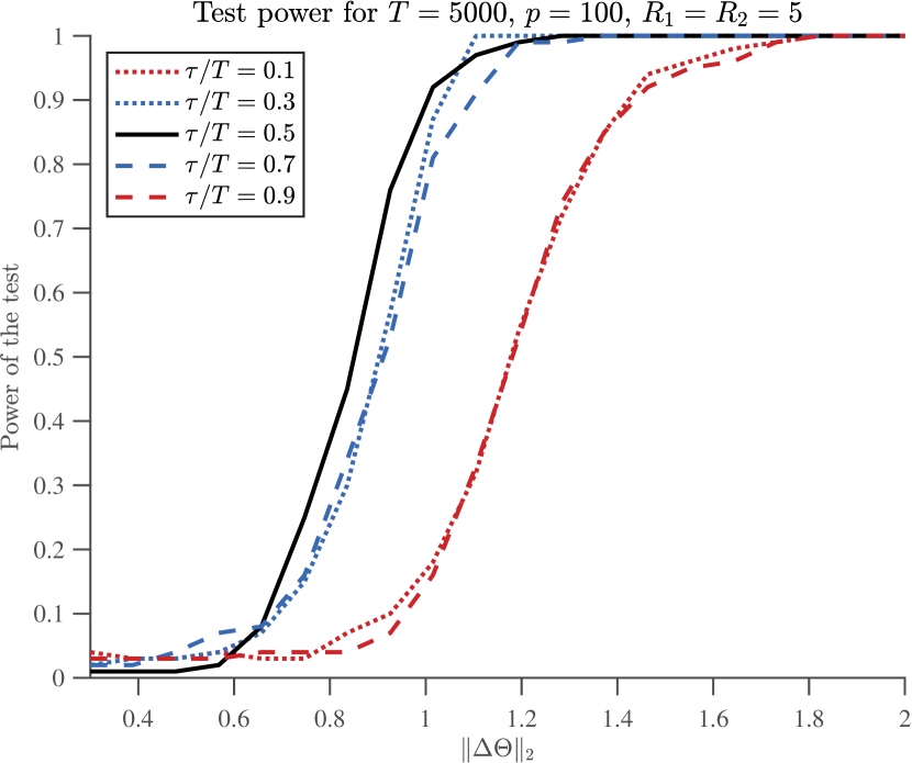
Figure 4: Dependence of the test power on different locations of the change-point

Finally, we consider $T=5000$ observations with fixed values $\gamma_{1}=\gamma_{2}=0.9$ and varying matrix ranks $R_{1}=R_{2}=R\in\{5,9,17,25\}$. The results in Fig. 5 demonstrate that the detection is easier for smaller rank of the matrices which is in line with the obtained detection rate of order $Rp/T$.

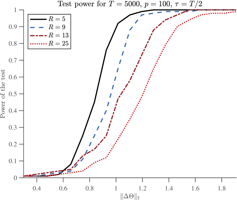
Figure 5: The test power depending on rank of the transition matrices

References

- Ahn and Reinsel, (1988) Ahn, S. K. and Reinsel, G. C. (1988). Nested reduced-rank autogressive models for multiple time series. Journal of the American Statistical Association, 83(403):849–856.
- Alquier et al., (2020) Alquier, P., Bertin, K., Doukhan, P., and Garnier, R. (2020). High-dimensional VAR with low-rank transition. Stat. Comput., 30(4):1139–1153.
- Aue et al., (2009) Aue, A., Hörmann, S., Horváth, L., and Reimherr, M. (2009). Break detection in the covariance structure of multivariate time series models. The Annals of Statistics, 37(6B):4046 – 4087.
- Bai et al., (2020) Bai, P., Safikhani, A., and Michailidis, G. (2020). Multiple Change Points Detection in Low Rank and Sparse High Dimensional Vector Autoregressive Models. IEEE Transactions on Signal Processing, 68:3074–3089.
- Bai et al., (2022) Bai, P., Safikhani, A., and Michailidis, G. (2022). Multiple change point detection in reduced rank high dimensional vector autoregressive models. Journal of the American Statistical Association, 0(ja):1–42.
- Basseville and Nikiforov, (1993) Basseville, M. and Nikiforov, I. V. (1993). Detection of Abrupt Changes: Theory and Application. Prentice-Hall, Inc., USA.
- Basu et al., (2019) Basu, S., Li, X., and Michailidis, G. (2019). Low rank and structured modeling of high-dimensional vector autoregressions. IEEE Transactions on Signal Processing, 67(5):1207–1222.
- Basu and Michailidis, (2015) Basu, S. and Michailidis, G. (2015). Regularized estimation in sparse high-dimensional time series models. The Annals of Statistics, 43(4):1535 – 1567.
- Carpentier and Nickl, (2015) Carpentier, A. and Nickl, R. (2015). On signal detection and confidence sets for low rank inference problems. Electronic Journal of Statistics, 9(2):2675 – 2688.
- Fan et al., (2010) Fan, J., Lv, J., and Qi, L. (2010). Sparse High Dimensional Models in Economics. SSRN Electronic Journal.
- Gorrostieta et al., (2013) Gorrostieta, C., Fiecas, M., Ombao, H., Burke, E., and Cramer, S. (2013). Hierarchical vector auto-regressive models and their applications to multi-subject effective connectivity. Frontiers in Computational Neuroscience, 7.
- Ingster and Suslina, (2003) Ingster, Y. I. and Suslina, I. A. (2003). Nonparametric Goodness-of-Fit Testing Under Gaussian Models. Springer New York.
- Ji and Ye, (2009) Ji, S. and Ye, J. (2009). An accelerated gradient method for trace norm minimization. In International Conference on Machine Learning, pages 457 – 464. ACM.
- Khan et al., (2020) Khan, F., Saeed, A., and Ali, S. (2020). Modelling and forecasting of new cases, deaths and recover cases of COVID-19 by using Vector Autoregressive model in Pakistan. Chaos, Solitons & Fractals, 140:110189.
- Liu et al., (2021) Liu, H., Gao, C., and Samworth, R. J. (2021). Minimax rates in sparse, high-dimensional change point detection. The Annals of Statistics, 49(2):1081–1112.
- Lütkepohl, (2005) Lütkepohl, H. (2005). New Introduction to Multiple Time Series Analysis. Springer.
- Melnyk and Banerjee, (2016) Melnyk, I. and Banerjee, A. (2016). Estimating structured vector autoregressive models. In Balcan, M. F. and Weinberger, K. Q., editors, Proceedings of The 33rd International Conference on Machine Learning, volume 48 of Proceedings of Machine Learning Research, pages 830–839, New York, New York, USA. PMLR.
- Michel and Murray, (2012) Michel, C. M. and Murray, M. M. (2012). Towards the utilization of eeg as a brain imaging tool. NeuroImage, 61(2):371–385.
- Negahban and Wainwright, (2011) Negahban, S. and Wainwright, M. J. (2011). Estimation of (near) low-rank matrices with noise and high-dimensional scaling. Ann. Statist., 39(2):1069–1097.
- Reinsel and Velu, (1998) Reinsel, G. C. and Velu, R. P. (1998). Multivariate Reduced-Rank Regression: Theory and Applications. ISBN: 9781475728538 OCLC: 1159215349.
- Rump, (2018) Rump, S. M. (2018). Estimates of the determinant of a perturbed identity matrix. Linear Algebra and its Applications, 558:101–107.
- Safikhani and Shojaie, (2022) Safikhani, A. and Shojaie, A. (2022). Joint structural break detection and parameter estimation in high-dimensional nonstationary var models. Journal of the American Statistical Association, 117(537):251–264.
- She et al., (2015) She, Y., He, Y., Li, S., and Wu, D. (2015). Joint association graph screening and decomposition for large-scale linear dynamical systems. IEEE Transactions on Signal Processing, 63(2):389–401.
- Stock and Watson, (2001) Stock, J. H. and Watson, M. W. (2001). Vector autoregressions. Journal of Economic Perspectives, 15(4):101–115.
- Tippett et al., (2000) Tippett, M. K., Cohn, S. E., Todling, R., and Marchesin, D. (2000). Conditioning of the stable, discrete-time lyapunov operator. SIAM Journal on Matrix Analysis and Applications, 22(1):56–65.
- Velu et al., (1986) Velu, R. P., Reinsel, G. C., and Wichern, D. W. (1986). Reduced rank models for multiple time series. Biometrika, 73(1):105–118.
- Vershynin, (2018) Vershynin, R. (2018). High-Dimensional Probability: An Introduction with Applications in Data Science. Cambridge Series in Statistical and Probabilistic Mathematics. Cambridge University Press.
- Wang and Tsay, (2021) Wang, D. and Tsay, R. S. (2021). Rate-optimal robust estimation of high-dimensional vector autoregressive models.
- Wang et al., (2019) Wang, D., Yu, Y., Rinaldo, A., and Willett, R. (2019). Localizing changes in high-dimensional vector autoregressive processes.
- Wild et al., (2010) Wild, B., Eichler, M., Friederich, H.-C., Hartmann, M., Zipfel, S., and Herzog, W. (2010). A graphical vector autoregressive modelling approach to the analysis of electronic diary data. BMC Medical Research Methodology, 10(1):28.