On the dual advantage of placing observations through forward sensitivity analysis

Abstract

The four-dimensional variational data assimilation methodology for assimilating noisy observations into a deterministic model has been the workhorse of forecasting centers for over three decades. While this method provides a computationally efficient framework for dynamic data assimilation, it is largely silent on the important question concerning the minimum number and placement of observations. To answer this question, we demonstrate the dual advantage of placing the observations where the square of the sensitivity of the model solution with respect to the unknown control variables, called forward sensitivities, attains its maximum. Therefore, we can force the observability Gramian to be of full rank, which in turn guarantees efficient recovery of the optimal values of the control variables, which is the first of the two advantages of this strategy. We further show that the proposed strategy of placing observations has another inherent optimality: the square of the sensitivity of the optimal estimates of the control with respect to the observations (used to obtain these estimates) attains its minimum value, a second advantage that is a direct consequence of the above strategy for placing observations. Our analytical framework and numerical experiments on linear and nonlinear systems confirm the effectiveness of our proposed strategy.

Keywords optimal sensor placement, forward sensitivity analysis, dynamic data assimilation, inverse problems, estimation, control

1 Introduction

Estimating the unknown parameters and initial/boundary conditions (collectively known as the control) of a dynamic model based on a finite set of noisy observations constitutes an important class of inverse problems of interest in a variety of disciplines [1, 2, 3, 4, 5, 6, 7, 8, 9, 10, 11, 12, 13]. At its core, this class of inverse problems gives rise to at least four question levels: (1) observability, (2) algorithmic path to estimate the model control, (3) observation count and placement of observation, and (4) assessing the quality of the estimates. At the first level, the observability question may be stated as follows: given the model dynamics and the observation operator, which relates the state of the dynamics to the observable, under what condition is it possible to estimate the unknowns based on a finite set of noisy observation? In a fundamental paper, Kalman [14] first provided a binary yes or no answer to this question based on the rank of the observability matrix derived from the linear model dynamics and the linear observation operator. Since then, this basic rank condition has been extended in several directions, including local and global observability of nonlinear systems [15, 16]. Furthermore, building upon the traditions in stability theory [17], researchers have proposed the concept of the degree of observability and scalar measures to quantify this degree [18, 19, 20, 21].

At the second level, given that a system is observable, the question is: what is an efficient algorithmic pathway to compute the estimates of the unknowns? Within the context of geosciences, a variational framework known as the four-dimensional variational data assimilation (4-D VAR) provides an answer in two steps. In the first step, a cost functional is defined by the weighted sum of squared differences between the actual and model counterpart of the observation at the time of the observation. The gradient of this cost functional (also known as the adjoint gradient) is computed using a forward run of the model and a backward sweep of its adjoint model. This process is referred to as the adjoint method (refer to Chapters 22-25 in Lewis et al. [4] for details). In the second step, this gradient is used in a minimization algorithm (Chapters 9-12, Lewis et al. [4]) to find an update of the control. These two steps are repeated until the desired convergence is reached.

The 4-D VAR based approach has been the workhorse of weather forecasting centers around the world since its introduction [22]. Despite its grand success in delivering forecast products for public consumption for decades, the 4-D VAR framework works with a given set of observations and is largely silent on the third level of inquiry, namely, what is the minimum number of observations required and their placement in the spatiotemporal domain to maximize the effectiveness of computing the estimates? At this juncture, it is useful to review the impact of the number of observations in general. Thanks to advances in the sensor, wireless communication, mass storage, and powerful computing technologies, we are steadily moving away from data-sparse to data-rich regimes. The ability to sample spatiotemporal fields at very high frequency (resulting from ever decreasing sampling intervals) has resulted in truly large datasets that are several orders of magnitude greater than what was available a decade ago. This growth has resulted in two side effects. First, the data exhibit very high correlations, which implies that more data does not translate into more information. Second, it is computationally demanding to ingest all the available data into an assimilation algorithm. These latter considerations highlight the importance of identifying smaller and independent subsets of observations to be used in estimation, which has resulted in a growing body of literature on “thinning” and creating of “super observations” [23].

In Lakshmivarahan et al. [24, 25], a strategy for answering this third level of question within the 4-D VAR framework was provided for the first time. An analysis based on the forward sensitivity method (FSM) has shown that the observability Gramian, $G$, is a good approximation to the Hessian of the cost function (it is exact for the linear case). In addition, the observability Gramian admits an additive decomposition: $G=\sum_{i=1}^{N}G_{i}$, where $G_{i}$ is the contribution to the overall Gramian at the $i^{th}$ observation time and $N$ is the number of observations. While each of these components is symmetric and positive semi-definite, it is shown in [24, 25] that we can indeed force the Gramian $G$ to be positive definite by placing the $N=(n+p)$ observations where the squares of the forward sensitivities of the model solution (with respect to $n$ components of the initial condition and $p$ parameters including the boundary conditions) attain their maxima. This strategy avoids flat patches in the cost functional by bounding the norm of the adjoint gradient away from zero. This is the first of the two advantages referred to in the title of this paper. The papers by Lewis et al. [26, 27] and Ahmed et al. [28, 29] contain several applications of this strategy.

At the fourth question level, the emphasis shifts to analyzing the quality of the resulting estimates of the control variables. There are two primary ways to approach this question. The first is to theoretically quantify the asymptotic distribution of the estimates by letting the number of observations increase without bounds. Within the context of time series analysis dealing with linear, discrete time, and stochastic dynamic models of the auto regressive integrated moving average (ARIMA) types, there is vast literature relating to the asymptotic analysis of the estimates of the parameters of these models [30, 31]. Likewise, there is a large body of results relating to static nonlinear models [32, 33]. But to our knowledge, there is no such theory of estimates for large-scale nonlinear dynamic models of interest in the geosciences. In the absence of such a statistical theory, we settle for the next best option—an analytical approach to quantify the sensitivity of the estimates with respect to the observations. This quantity is particularly important when the given dynamic model exhibits high sensitivity to errors in the control. In this paper, we prove that the sensitivity of the estimates with respect to the observations attains their minimum value when we place the observations where the squares of the forward sensitivities are maximized as in [24, 25]. The positive definite Gramian resulting from the proposed strategy for observation placement determines the control estimates that exhibit the smallest possible sensitivity to observations. This is the second advantage of setting the observation placement strategy using the forward sensitivity analysis.

1.1 Historical remarks

The four levels of inquiry described above have natural connections to many different areas of the data assimilation and parameter estimation in dynamical systems literature spanning several decades. First is the fundamental structural identifiability question examined by Bellman and Astrom [34], where it was shown that certain types of model parametrization do not admit a unique solution to the parameter estimation problem. Furthermore, there is extensive literature on lumped parameter system identification [35] and adaptive control [36] dealing with parameter estimation. A recent paper by Villaverde [37] contains an extensive analysis of observability and identification of nonlinear systems of interest in mathematical biology.

Within the parlance of distributed parameter systems, especially in the context of process control in chemical engineering, there is an extensive body of results relating to parameter estimation, placement of observations, and analysis of the sensitivity of parameter estimates with respect to observations. We refer to the monograph by Ucinski [38] and papers by Alaña [39] and Christopher and Fathalla [40] for more details. The results in the present paper share some connections with the developments in Christopher and Fathalla [40] and Alaña [39]. Nonetheless, these two papers deal only with parameter estimation for distributed parameter systems, while the present study addresses the mutual estimation of initial conditions and parameters (denoted as control) in the same footing for systems described by ordinary/partial differential equations (ODEs/PDEs). For general treatment of sensitivity-based methods, we refer to the foundational works by Cacuci and co-workers [41, 42]. Some of the ideas developed in the current study can be also connected to the vast and growing literature on adjoint-based analysis of targeted observations and adaptive observations [43, 44, 45, 46, 47, 48] as well as ensemble-based approaches to observation impact analysis [49, 50].

1.2 Significance

This paper addresses, for the first time, key questions related to the simultaneous estimate of unknown initial conditions and model parameters in variational data assimilation frameworks. The main questions that we answer correspond to observation count and optimal placement as well as the subsequent quality of the inverse problem solution. We present a mathematically concrete strategy for selecting the observation locations by tracking the model forward sensitivity metrics, namely the forecast sensitivity with respect to the initial condition and to the model parameters. Because these sensitivities can generally be positive or negative, we opt for placing the observations at points where the squares of the forward sensitivities attain their maximum. We support the proposed observation placement strategy with a clear theoretical analysis to understand the consequences of this strategy. In particular, we demonstrate both theoretically and empirically that the advocated observation placement methodology has two main advantages as follows.

First, by placing the observations where the forward sensitivities are maximized, we enforce the observability Gramian matrix to be positive definite. We illustrate that this Gramian is closely related to the adjoint gradient of the cost function. Specifically, a positive definite observability Gramian leads to non-zero values of the adjoint gradient norm, which accelerates the optimization algorithm that is used to estimate the unknown initial conditions and model parameters. We highlight that the choice of observation locations controls the shape of the resulting cost function (defined using a weighted sum of the squared differences between the collected measurements and the model counterpart of the observation). Placing the observations using the presented forward sensitivity analysis avoids flat regions of the cost function, which would negatively affect the algorithm convergence.

Second, we demonstrate that the optimal estimates of the initial conditions and model parameters are sensitive to the locations where measurements are collected. More specifically, we prove that the sensitivities of those estimates (with respect to the observations themselves) reach their minimum values when the forecast sensitivities (with respect to the control) reach their maximum values. In other words, by placing the observations where the squares of forecast sensitivities with respect to the unknown control are maximized, we guarantee that the solution of the inverse problem is the most robust to small perturbations in observation values. This second result has significant merit in practice, considering the inevitably noisy sensor data with different levels of uncertainties. We back up the analytical framework with numerical experiments using representative systems exhibiting linear and nonlinear dynamics with unknown initial conditions and model parameters.

1.3 Organization of the paper

In Section 2, we provide a succinct version of the statement of the inverse problem of interest in this paper. In Section 3, we introduce an optimal observation placement strategy using the forward sensitivity analysis that links the observability Gramian and the adjoint gradient. We lay out the analytical framework for defining the dual advantages of the proposed observation placement strategy in Section 3 and Section 4. In the latter, we provide a theoretical analysis for evaluating the sensitivity of the control estimates with respect to the observation. In Section 5, we illustrate the theory of observation placement through the forward sensitivity analysis using examples corresponding to scalar linear and nonlinear dynamical systems with two elements of control—the initial condition and model parameterization—as well as two systems governed by PDEs in one and two spatial dimensions. We draw concluding remarks about the derived optimality conditions for observation placement and the associated twin advantages in Section 6.

2 Mathematical Preliminaries

We start with a description of the model. Our primary goal is to bring out the beauty and elegance of the underlying ideas and results using simple, easily understandable models. Therefore, we first derive the analytical framework and perform the theoretical analysis using a scalar (one-dimensional) dynamical system with a single parameter. After that, we provide extensions and insights regarding the higher-dimensional cases.

2.1 Model

Let $\mathcal{I}\subset\mathbb{R}$ and $\mathcal{P}\subset\mathbb{R}$ be two subsets of the real line representing the set of all allowed values of the initial condition $x(0)$ and parameter $\alpha$ of a dynamic model, respectively. The state, $x(t)\in\mathbb{R}$, evolves according to the following nonlinear, time-invariant, ordinary differential equation (ODE):

$$\dot{x}=f(x,\alpha),$$ (1)

where $f:\mathbb{R}\times\mathbb{R}\to\mathbb{R}$, $x(0)\in\mathcal{I}$, and $\alpha\in\mathcal{P}$. Henceforth, the triplet $(f,\mathcal{I},\mathcal{P})$ denotes a class of models of interest. Let $x(t)=x(t,x_{0},\alpha)$ denote the solution of Eq. 1. Because the solution depends on $x(0)$ and $\alpha$, the vector $c=(x_{0},\alpha)^{\mkern-1.5mu\mathsf{T}}\in\mathbb{R}^{2}$ is called the control and in the rest of the paper, we use $x(t)$ and $x(t,c)$ interchangeably.

For the FSM theoretical analysis that we carry out, in addition to the existence and uniqueness of the solution of Eq. 1, we are also interested in the smoothness of the solution regarding the existence of continuous (mixed) partial derivatives of $x(t)$ with respect to $x_{0}$ and $\alpha$ of order $K\geq 1$. In this context, we recall that a function $g:\mathbb{R}\to\mathbb{R}$ belongs to the class $C^{k}$ if $g$ and its first $K$ derivatives are continuous. According to a theorem in Chapter 2, Section 7 in Arnold [51], the solution $x(t)$ of Eq. 1 belongs to $C^{K}$ for some integer $K\geq 1$ if $f(x,\alpha)$ belongs to the same class $C^{K}$. We define $\mathcal{S}(f)=\{x(t,c)|c\in\mathcal{I}\times\mathcal{P}\}$ as the ensemble of all possible solutions of Eq. 1 for a given $f(x,\alpha)\in C^{K}$, where $x(0)$ and $\alpha$ are varied in $\mathcal{I}$ and $\mathcal{P}$. For example, if $\dot{x}=ax$, $\mathcal{I}=\mathbb{R}^{+}$ (the positive real line), and $\mathcal{P}=[-1,1]$, then $\mathcal{S}(f=ax)$ is the set of all exponentials of the form $x(t)=e^{at}x(0)$ where $a\in[-1,1]$ and $x(0)\in\mathbb{R}^{+}$.

The forward sensitivities of the solution at time $t>0$ with respect to the initial condition $x_{0}$ and parameter $\alpha$ can be defined as follows:

$$u(t)=\dfrac{\partial x(t)}{\partial x_{0}},\quad\text{and}\quad v(t)=\dfrac{\partial x(t)}{\partial\alpha}.$$ (2)

By differentiating Eq. 1 with respect to $x(0)$ and $\alpha$, it can be verified that $u(t)$ and $v(t)$ evolve according to linear non-autonomous systems given by

$$\dot{u}(t) =D_{f}(x(t))u(t),\quad u(0)=1,$$ (3)

$$\dot{v}(t) =D_{f}(x(t))v(t)+D_{f}^{\alpha}(x(t)),\quad v(0)=0,$$

where

$$D_{f}(x)=\dfrac{\partial f}{\partial x},\quad\text{and}\quad D_{f}^{\alpha}(x)=\dfrac{\partial f}{\partial\alpha}.$$ (4)

We refer to [52, 53] for the derivation of the forward sensitivity method. By solving Eqs. 1 and 3, we can compute the evolution of the solution $x(t)$ and its sensitivities with respect to time.

2.2 Observations

It is assumed that there is an underlying physical process and that the model $(f,\mathcal{I},\mathcal{P})$ defined above is faithful to this process in the sense that all the large features of the process are captured by the model. Let $\bar{x}(t)$ for $t\geq 0$ be the true (yet unknown) state of the system under consideration. It is often the case that we may not be able to observe $\bar{x}(t)$ but only a certain function of it at discrete points in time and space. In addition, observations get corrupted by device errors and measurement noise that is usually modeled as additive Gaussian noise with zero mean and known variance $\sigma^{2}$.

Let $h:\mathbb{R}\to\mathbb{R}$, where $h\in C^{K}$, be the function that maps the true state $\bar{x}(k)$ into the observables $z(k)$ as follows:

$$z(k)=h(\bar{x}(k))+\eta(k),$$ (5)

where $k$ is the discrete time index and $\eta(k)$ is white noise, meaning that the observation $z(k)$ contains noisy information about the (unknown) true state. Finally, we define $\mathcal{O}=\{z(k_{i})|1\leq i\leq N\}$ as the set of $N$ observations at discrete times given by $0\leq k_{1}\leq k_{2}\leq\dots\leq k_{N}$.

2.3 Statement of the problem

Given the model, Eq. 1, and the set $\mathcal{O}$ of observations, our goal is to find the initial condition $x(0)\in\mathcal{I}$ and parameter $\alpha\in\mathcal{P}$ such that the solution $x(t)$ of Eq. 1 starting with $c=(x_{0},\alpha)^{\mkern-1.5mu\mathsf{T}}$ minimizes the weighted sum of squared error between $z(k)$ and $h(x(k))$. To this end, we define a cost functional as follows:

$$J(c)=\dfrac{1}{2\sigma^{2}}\sum_{i=1}^{N}[z(k_{i})-h(x(k_{i}))]^{2}.$$ (6)

The problem of minimizing $J(c)$ can be solved by computing the gradient $\nabla J(c)\in\mathbb{R}^{2}$, called the adjoint gradient, and the minimizer can be sought by using the adjoint gradient in an iterative minimization algorithm [4].

3 Observability Gramian and Adjoint Gradient

We first examine the fine structure of the adjoint gradient and its dependence on the observability Gramian using the forward sensitivity analysis [24, 25]. Let $x(t)$ and $\bar{x}(t)$ be the solution of Eq. 1 starting from $c=(x_{0},\alpha)^{\mkern-1.5mu\mathsf{T}}$ and $\bar{c}=(\bar{x}_{0},\bar{\alpha})^{\mkern-1.5mu\mathsf{T}}$, respectively, where the perturbations in the initial conditions and the parameter are given by:

$$\delta x(0)=\bar{x}_{0}-x_{0},\qquad\delta\alpha=\bar{\alpha}-\alpha,\qquad\delta c=(\delta x_{0},\delta\alpha)^{\mkern-1.5mu\mathsf{T}}.$$ (7)

The induced first variation in the solution of Eq. 1 resulting from the initial perturbation $\delta c$ in the control $c$ is defined as follows:

$$\delta x(k)=\bar{x}(k)-x(k).$$ (8)

The forecast error, also known as the innovation, can be thus computed as follows:

$$e(k)=z(k)-h(x(k))=h(\bar{x}(k))-h(x(k))+\eta(k).$$ (9)

Because $h\in C^{K}$ and by substituting Eq. 8 in Eq. 9 and applying first-order Taylor expression, the deterministic component of $e(k)$ can be written as follows:

$$e(k)=D_{h}(x(k))\delta x(k),$$ (10)

where $D_{h}(x)=\dfrac{\partial h}{\partial x}$. Also, recall from first principles $\delta x(k)=u(k)\delta x(0)+v(k)\delta\alpha=F\delta c$, where

$$F=[u,v]\in\mathbb{R}^{1\times 2}.$$ (11)

From Eqs. 10 and 11, we get:

$$e(k)=D_{h}(x(k))F\delta c.$$ (12)

Now, let $\delta J$ be the induced variation in $J(c)$ resulting from the initial perturbation $\delta c$ in $c$. Then, it can be verified that [4]:

$$\delta J=-\dfrac{1}{\sigma^{2}}\sum_{i=1}^{N}e(k_{i})D_{h}(x(k_{i}))\delta x(k)=-\dfrac{1}{\sigma^{2}}\sum_{i=1}^{N}e(k_{i})D_{h}(x(k_{i}))F\delta c.$$ (13)

Substituting for $e(k)$ using Eq. 12, we get an alternative expression for $\delta J$ as follows:

$$\delta J=-\dfrac{1}{\sigma^{2}}\delta c^{\mkern-1.5mu\mathsf{T}}G\delta c,$$ (14)

where

$$G=\sum_{i=1}^{N}G_{i}\in\mathbb{R}^{2\times 2}\quad\text{and }G_{i}=F^{\mkern-1.5mu\mathsf{T}}D_{h}^{2}(x(k_{i}))F\in\mathbb{R}^{2\times 2}.$$ (15)

The $2\times 2$ matrix $G$ is known as the observability Gramian, which is always symmetric and, in general, positive semi-definite. The problem of placing observations is determining the minimum number of observations required and where to place them in order to make $G$ positive definite. To this and, we rewrite $G$ as

$$G=\sum_{i=1}^{N}D^{2}_{h}(x(k_{i}))\begin{bmatrix}u^{2}(k_{i})&u(k_{i})v(k_{i})\\ v(k_{i})u(k_{i})&v^{2}(k_{i})\end{bmatrix}.$$ (16)

Under the regularity assumption that $D_{h}(x)$ does not vanish along the solution in the set $\mathcal{S}(f)$ in Section 2.1 and that $D^{2}_{h}(x(k_{i}))$ is positive, a good rule is to place the observations where $u^{2}(k_{i})$ and $v^{2}(k_{i})$ attain their maximum value. Clearly, in this case, we would need only $N=2$ observations: one at the maximum of $u^{2}(k)$ and another at the maximum of $v^{2}(k)$. We note that by placing the observations where $u^{2}$ and $v^{2}$ attain their maximum values, the observability Gramian $G$ becomes positive definite, which in turn bounds the norm of the adjoint gradient away from zero (see Eq. 14). By doing so, flat patches of the cost functional are avoided and the convergence of the optimization algorithm is improved.

4 Natural Consequence of the Placement Strategy: A Theoretical Analysis

The strategy of placing observations where the square of the forward sensitivities attains a maximum has another natural optimality property. To examine this inherent optimality, we seek an expression for the adjoint gradient starting from the fact that $\delta J=\langle\nabla J(c),\delta c\rangle$ and at the extremum $\nabla J(c)=0$, where $\langle\cdot,\cdot\rangle$ denotes the inner product. Combining this with Eq. 13, we obtain the following conditions for the optimality:

$$g_{1} =\dfrac{\partial J}{\partial x_{0}}=-\dfrac{1}{\sigma^{2}}\sum_{i=1}^{N}(z(k_{i})-h(x(k_{i})))D_{h}(x(k_{i}))U(k_{i})=0,$$ (17)

$$g_{2} =\dfrac{\partial J}{\partial\alpha}=-\dfrac{1}{\sigma^{2}}\sum_{i=1}^{N}(z(k_{i})-h(x(k_{i})))D_{h}(x(k_{i}))V(k_{i})=0.$$ (18)

Because the maps $f$ in Eq. 1 and $h$ in Eq. 5 are fixed, it can be verified that $g_{i}=g_{i}(z,x_{0},\alpha)$ is a function of $z,x_{0},\alpha$, where $z=(z(k_{1}),\dots,z(k_{N}))^{\mkern-1.5mu\mathsf{T}}\in\mathbb{R}^{N}$. In the following analysis, we consider two cases corresponding to a single observation with a linear observation operator and multiple observations with a generic nonlinear observation operator. Although the former is a subset of the latter, we begin with the simpler case to define the main quantities that enable us to understand and analyze the second advantage of the given observation placement strategy.

4.1 Case 1: scalar dynamical systems with unknown initial condition

In the first case, we consider a single observation (i.e., $N=1$), known model parameter $\alpha$, and unknown initial condition $x_{0}$. Moreover, we assume that the model state is directly observable (i.e., $h(x)=x$, and $D_{h}(x)=1$). Thus, the optimality condition in Eq. 17 can be reduced to the following:

$$-\sigma^{2}g_{1}(z,k)=[z(k)-x(k)]u(k)=0.$$ (19)

Because $f$, $h$, and $\alpha$ are invariant, solving Eq. 19 yields an optimal value of $x_{0}=x_{0}(z,k)$ as a function of $z(k)$ and $k$. We are interested in quantifying the sensitivity of the optimal estimate of $x_{0}$ with respect to the observation $z$ at time $k$ as follows:

$$y(k)=\dfrac{\partial x_{0}(z,k)}{\partial z}.$$ (20)

To this end, by differentiating both sides of Eq. 19 with respect to $z=z(k)$, we obtain

$$0=-\sigma^{2}\dfrac{\partial g_{1}}{\partial z}=[1-u(k)\dfrac{\partial x_{0}}{\partial z}]u(k)+[z(k)-x(k)]\dfrac{\partial u(k)}{\partial x_{0}}\dfrac{\partial x_{0}}{\partial z}.$$ (21)

Solving Eq. 21, we obtain the required expression:

$$y(k)=\dfrac{\partial x_{0}}{\partial z}=\dfrac{u(k)}{u^{2}(k)-e(k)\dfrac{\partial u(k)}{\partial x_{0}}}.$$ (22)

A little reflection reveals that when $x(t)$ is the optimal trajectory, $e(k)=z(k)-x(k)$ is small and can be set to zero in Eq. 22 to give the following approximation:

$$y(k)=\dfrac{\partial x_{0}}{\partial z}\approx\dfrac{u(k)}{u^{2}(k)}=\dfrac{sign(u(k))}{|u(k)|}.$$ (23)

Equation 23 implies that $y(k)$ is minimum where $u^{2}(k)$ attains its maximum value. In other words, placing the single observation at time $k^{*}$, where $u^{2}(k)$ attains its maximum value, ensures that the sensitivity $y(k^{*})$ takes its minimum value.

For the complementary case when $\alpha$ is not known but $x_{0}$ is known, the optimality condition in Eq. 18 becomes:

$$0=\sigma^{2}g_{2}(z,k)=[z(k)-x(k)]v(k).$$ (24)

Through similar arguments, it can be verified that the optimal $\alpha$ that satisfies Eq. 24 is a function of $z$ and $k$. We define the sensitivity of the optimal $\alpha$ with respect to the observation $z(k)$ as follows:

$$w(k)=\dfrac{\partial\alpha(z,k)}{\partial z}.$$ (25)

Differentiating Eq. 24 with respect to $z$ and simplifying using the same reasoning used in obtaining Eq. 23, we get:

$$w(k)=\dfrac{v(k)}{v^{2}(k)-e(k)\dfrac{\partial v(k)}{\partial\alpha}}\approx{\color[rgb]{0,0,0}\dfrac{sign(v(k))}{|v(k)|}}.$$ (26)

Thus, $w(k)$ takes on its minimum value at $k=k^{*}$ where $v^{2}(k)$ attains its maximum value, implying that the proposed observation placement strategy (i.e., where $v^{2}(k)$ attains its maximum value) leads to the minimum value of $w(k)$.

4.2 Case 2: scalar dynamical systems with unknown parameter and initial condition

Next, we extend our theoretical analysis to consider the simultaneous estimation of unknown initial conditions and model parameters in the general case of multiple observations and arbitrary observation operators. Solving Eqs. 17 and 18, it follows that the optimal estimates $x_{0}=x_{0}(z)$ and $\alpha=\alpha(z)$ are functions of the observations, where $z=(z(k_{1}),\dots,z(k_{N}))^{\mkern-1.5mu\mathsf{T}}\in\mathbb{R}^{N}$. Let $x=x(t,x_{0}(z),\alpha(z))$ be the optimal solution of Eq. 1, starting from the optimal control $c(z)=(x_{0}(z),\alpha(z))^{\mkern-1.5mu\mathsf{T}}$. In addition, we suppose that $u(t)=u(t,x_{0}(z),\alpha(z))$, $v(t)=v(t,x_{0}(z),\alpha(z))$, and $D_{h}(x(t))$ are evaluated along the optimal trajectory $x(t)$.

To bring out the key ideas and simplify the algebra, without loss of generality, we set $N=2$ and denote $k_{i}$ by $i$. Then, the optimality conditions given by Eqs. 17 and 18 for $i=1,2$ can be rewritten as follows:

$$\sigma^{2}g_{1} =H_{1}=H_{11}+H_{12}=0,$$ (27)

$$\sigma^{2}g_{2} =H_{2}=H_{21}+H_{22}=0,$$

where

$$H_{11} =[z(1)-h(x(1))]D_{h}(x(1))u(1), \quad H_{12} =[z(2)-h(x(2))]D_{h}(x(2))u(2),$$ (28)

$$H_{21} =[z(1)-h(x(1))]D_{h}(x(1))v(1), \quad H_{22} =[z(2)-h(x(2))]D_{h}(x(2))v(2),$$ (29)

where $z(i)$, $x(i)$, $u(i)$, and $v(i)$ are the values of the respective quantities evaluated at time $t=k_{i}=i$, $1\leq i\leq 2$. We define the sensitivities of $x_{0}(z)$ and $\alpha(z)$ with respect to $z_{i}$ for $i=1,2$ as follows:

$$y_{i}=\dfrac{\partial x_{0}(z)}{\partial z_{i}},\quad\text{and }w_{i}=\dfrac{\partial\alpha(z)}{\partial z_{i}}.$$ (30)

Our goal is to relate the sensitivities in Eq. 30 to the forecast sensitivities $u(k)$ and $v(k)$. As illustrated in Case 1 above, this can be accomplished by computing the derivatives of $H_{i}=0$ in Eq. 27 with respect to $z_{i}$ for $1\leq i\leq 2$, which, when simplified, gives the sought after relation. The details of this derivation are given in Appendix A. From Eq. 74–Eq. 75 of this appendix, we get the following:

$$G\begin{bmatrix}y_{i}\\ w_{i}\end{bmatrix}=D_{h}(i)\begin{bmatrix}u_{i}\\ v_{i}\end{bmatrix},$$ (31)

for $i=1,2$, where $G=G_{1}+G_{2}$, $F(i)=[u(i),v(i)]\in\mathbb{R}^{1\times 2}$. The observability Gramian decomposition $G_{i}$ can be evaluated as follows:

$$G_{i}=F^{\mkern-1.5mu\mathsf{T}}(i)D_{h}^{2}(i)F(i)$$ (32)

where it is assumed that $D_{h}^{2}(i)=D_{h}^{2}(x(i))>0$ along the trajectory of $x$ in Eq. 1. Consequently, the inverse of $G$ controls the behavior of $y_{i}$ and $w_{i}$. Setting $D_{h}^{2}(i)=d_{i}$ for simplicity in notation, it can be verified that

$$G=\begin{bmatrix}d_{1}^{2}u_{1}^{2}+d_{2}^{2}u_{2}^{2}&d_{1}^{2}u_{1}v_{1}+d_{2}^{2}u_{2}v_{2}\\ d_{1}^{2}u_{1}v_{1}+d_{2}^{2}u_{2}v_{2}&d_{1}^{2}v_{1}^{2}+d_{2}^{2}v_{2}^{2}\end{bmatrix}$$ (33)

and its determinant is given by

$$|G|=d_{1}^{2}d_{2}^{2}(u_{1}v_{2}-u_{2}v_{1})^{2}.$$ (34)

Because the sensitivities can generally be positive or negative, for definiteness, our strategy is based on the square of the sensitivities. Therefore, placing the first observation $z_{1}$ at the maximum value of $u_{1}^{2}$ and the second observation $z_{2}$ at the maximum value of $v_{2}^{2}$ maximizes $|G|$. This in turn reduces the magnitudes of $y_{i}$ and $w_{i}$ as desired, per Cramer’s rule. Table 1 provides expressions for $y(i)$ and $w(i)$ for $i=1,2$.

Remark 4.1 —

For an increased number of observations, it is crucial to guarantee that the observation placement strategy does not lead to a singular Gramian matrix. In Appendix B, we prove that the forecast sensitivities with respect to the initial condition and parameter cannot be linearly dependent and that the resulting Gramian is therefore non-singular.

Table 1: Expressions for $y(i)$ and $w(i)$ for $i=1,2$.

	$y$	$w$
$i=1$	$\dfrac{v_{2}(u_{1}v_{2}-u_{2}v_{1})}{|G|}$	$\dfrac{u_{2}(u_{2}v_{1}-u_{1}v_{2})}{|G|}$
$i=2$	$\dfrac{v_{1}(u_{2}v_{1}-u_{1}v_{2})}{|G|}$	$\dfrac{u_{1}(u_{1}v_{2}-u_{2}v_{1})}{|G|}$

4.3 Extensions to high-dimensional systems

We consider the case for which the state variable $\mathbf{x}$ is represented by a vector (i.e., $\mathbf{x}\in\mathbb{R}^{n}$, where $n$ is the number of degrees of freedom of the system) and $\boldsymbol{\alpha}\in\mathbb{R}^{p}$. The discrete-time version of the model in Eq. 1 for $\mathbf{x}\in\mathbb{R}^{n}$ can be written as follows:

$$\mathbf{x}_{k+1}=\boldsymbol{M}(\mathbf{x}_{k},\boldsymbol{\alpha}),$$ (35)

where $\boldsymbol{M}:\mathbb{R}^{n}\times\mathbb{R}^{p}\to\mathbb{R}^{n}$ defines the one-time step mapping defined by applying a temporal integration scheme (e.g., $\boldsymbol{M}(x_{k},\boldsymbol{\alpha})=\mathbf{x}_{k}+(t_{k+1}-t_{k})\boldsymbol{f}(\mathbf{x}_{k},\boldsymbol{\alpha})$ for a first-order Euler integrator). Equation 3 for the dynamics of $\mathbf{u}(t)\in\mathbb{R}^{n\times n}$ and $\mathbf{v}(t)\in\mathbb{R}^{n\times p}$ can be rewritten as follows:

$$\mathbf{u}_{k+1}=\mathbf{D}_{\mathbf{M}}(k)\mathbf{u}_{k},\qquad\text{and}\qquad\mathbf{v}_{k+1}=\mathbf{D}_{\mathbf{M}}(k)\mathbf{v}_{k}+\mathbf{D}_{\mathbf{M}}^{\boldsymbol{\alpha}}(\mathbf{x}_{k}),$$ (36)

where

$$\bigg{[}\mathbf{D}_{\mathbf{M}}(k)\bigg{]}_{i,j}=\dfrac{\partial M_{i}}{\partial x_{j}}\bigg{|}_{\mathbf{x}=\mathbf{x}_{k}},\qquad\text{and}\qquad\bigg{[}\mathbf{D}_{\mathbf{M}}^{\boldsymbol{\alpha}}(k)\bigg{]}_{i,j}=\dfrac{\partial M_{i}}{\partial\alpha_{j}}\bigg{|}_{\mathbf{x}=\mathbf{x}_{k}}.$$ (37)

Without loss of generality, we focus our analysis on estimating the model’s initial condition $\mathbf{x}_{0}$ from a set of measurements, $\mathbf{z}\in\mathbb{R}^{m}$, (i.e., the control is $\mathbf{c}=\mathbf{x}_{0}$).

4.3.1 Linear dynamics (vector)

We first consider a linear dynamical system:

$$\mathbf{x}_{k+1}=\mathbf{M}\mathbf{x}_{k},$$ (38)

where $\mathbf{M}\in\mathbb{R}^{n\times n}$ is a square matrix with rank $n$. Furthermore, we suppose that the measurement vector $\mathbf{z}\in\mathbb{R}^{m}$ is related to the state $\mathbf{x}$ by a linear operator $\mathbf{H}\in\mathbb{R}^{m\times n}$ as follows:

$$\mathbf{z}_{k}=\mathbf{H}\mathbf{x}_{k}+\boldsymbol{\eta}_{k},$$ (39)

where $\boldsymbol{\eta}_{k}\in\mathbb{R}^{m}$ represents an additive measurement noise. The cost function for the inverse problem can be written as:

$$J(\mathbf{c}) =\dfrac{1}{2}\sum_{i=1}^{N}[\mathbf{z}_{i}-\mathbf{H}\mathbf{x}_{i}]^{\mkern-1.5mu\mathsf{T}}R^{-1}[\mathbf{z}_{i}-\mathbf{H}\mathbf{x}_{i}].$$ (40)

From Eq. 38, we can relate the prediction $\mathbf{x}_{i}$ to the initial condition $\mathbf{x}_{0}=\mathbf{c}$ as $\mathbf{x}_{i}=\mathbf{M}^{i}\mathbf{x}_{0}=\mathbf{M}^{i}\mathbf{c}$ and $\mathbf{x}_{i}^{\mkern-1.5mu\mathsf{T}}=\mathbf{c}^{\mkern-1.5mu\mathsf{T}}(\mathbf{M}^{i})^{\mkern-1.5mu\mathsf{T}}=\mathbf{c}^{\mkern-1.5mu\mathsf{T}}(\mathbf{M}^{\mkern-1.5mu\mathsf{T}})^{i}$. We also note that the forward sensitivity of the model forecast with respect to its initial condition can be defined as $\mathbf{u}_{i}=\mathbf{M}^{i}$ because the model Jacobian is $\mathbf{D}_{\mathbf{M}}=\mathbf{M}$ and $\mathbf{u}_{0}=\mathbf{I}$ (the identity matrix). Therefore, Eq. 40 and its gradient can be rewritten as:

$$J(\mathbf{c}) =\dfrac{1}{2}\sum_{i=1}^{N}\bigg{[}\mathbf{z}_{i}^{\mkern-1.5mu\mathsf{T}}\mathbf{R}^{-1}\mathbf{z}_{i}-2\mathbf{z}_{i}^{\mkern-1.5mu\mathsf{T}}\mathbf{R}^{-1}\mathbf{H}\mathbf{M}^{i}\mathbf{c}+\mathbf{c}^{\mkern-1.5mu\mathsf{T}}\big{(}(\mathbf{M}^{\mkern-1.5mu\mathsf{T}})^{i}\mathbf{H}^{\mkern-1.5mu\mathsf{T}}\mathbf{R}^{-1}\mathbf{H}\mathbf{M}^{i}\big{)}\mathbf{c}\bigg{]},$$ (41)

$$\nabla_{\mathbf{c}}J =\sum_{i=1}^{N}[(\mathbf{M}^{\mkern-1.5mu\mathsf{T}})^{i}\mathbf{H}^{\mkern-1.5mu\mathsf{T}}\mathbf{R}^{-1}[\mathbf{H}\mathbf{M}^{i}\mathbf{c}-\mathbf{z}_{i}].$$ (42)

Setting the gradient $\nabla_{\mathbf{c}}J$ in Eq. 42 to zero, we get an optimal expression for $\mathbf{c}$ as follows:

$$\sum_{i=1}^{N}(\mathbf{M}^{\mkern-1.5mu\mathsf{T}})^{i}\mathbf{H}^{\mkern-1.5mu\mathsf{T}}\mathbf{R}^{-1}\mathbf{H}\mathbf{M}^{i}\mathbf{c}=\sum_{i=1}^{N}(\mathbf{M}^{\mkern-1.5mu\mathsf{T}})^{i}\mathbf{H}^{\mkern-1.5mu\mathsf{T}}\mathbf{R}^{-1}\mathbf{z}_{i}.$$ (43)

The observability Gramian is now defined as $\mathbf{G}=\sum_{i=1}^{N}\mathbf{G}_{i}$, where $\mathbf{G}_{i}=(\mathbf{M}^{\mkern-1.5mu\mathsf{T}})^{i}\mathbf{H}^{\mkern-1.5mu\mathsf{T}}\mathbf{R}^{-1}\mathbf{H}\mathbf{M}^{i}$. Thus, the optimal $\mathbf{c}$ is given by

$$\mathbf{c}=\mathbf{G}^{-1}\sum_{i=1}^{N}(\mathbf{M}^{\mkern-1.5mu\mathsf{T}})^{i}\mathbf{H}^{\mkern-1.5mu\mathsf{T}}\mathbf{R}^{-1}\mathbf{z}_{i}.$$ (44)

Differentiating both sides of Eq. 44 with respect to $\mathbf{z}_{i}$ yields the following expression for the sensitivity of the optimal estimate of the control $\mathbf{c}$ to the measurements:

$$\dfrac{\partial\mathbf{c}}{\partial\mathbf{z}_{i}}=\mathbf{G}^{-1}(\mathbf{M}^{\mkern-1.5mu\mathsf{T}})^{i}\mathbf{H}^{\mkern-1.5mu\mathsf{T}}\mathbf{R}^{-1}.$$ (45)

Maximizing the square of the forward sensitivity of the model forecast with respect to the control yields a Gramian matrix $\mathbf{G}$ with the largest determinant, which minimizes the sensitivity of the optimal estimate of the control to the actual measurements.

We note that the minimum number of observation times $N$ to yield a well-posed inverse problem is defined as $N=\dfrac{n}{m}$. However, we highlight that due to the existence of measurement noise and correlations between measurement components, a regularization is often imposed for the solution of the inverse problem. For the special case of $m=n$, we place a single measurement $\mathbf{z}_{i}\in\mathbb{R}^{n}$ at arbitrary time $i$. Assuming $\mathbf{H}=\mathbf{I}$ and $\mathbf{R}^{-1}=\dfrac{1}{\sigma^{2}}\mathbf{I}$, we get the following expressions for the Gramian and the sensitivity of the optimal estimate of the control $\mathbf{c}$ with respect to the measurement $\mathbf{z}_{i}$:

$$\mathbf{G}=\dfrac{1}{\sigma^{2}}(\mathbf{M}^{\mkern-1.5mu\mathsf{T}})^{i}\mathbf{M}^{i}\qquad\text{and}\qquad\dfrac{\partial\mathbf{c}}{\partial\mathbf{z}_{i}}=\mathbf{M}^{-i}.$$ (46)

As noted above, the forecast sensitivity with respect to the initial conditions can be written as $\mathbf{u}_{i}=\mathbf{M}^{i}$ in the linear dynamics case. Therefore, the sensitivity $\dfrac{\partial\mathbf{c}}{\partial\mathbf{z}_{i}}$ is inversely proportional to the sensitivity of $\mathbf{x}_{i}$ with respect to $\mathbf{c}$.

Remark 4.2 —

The system matrix $\mathbf{M}$ in Eq. 38 is a real matrix and it may or may not be diagonalizable. For the latter, it is similar to the Jordan normal form. For the case where $\mathbf{M}$ is diagonalizable, there exists a non-singular matrix $P$ such that

$$\Lambda=\mathbf{P}^{-1}\mathbf{M}\mathbf{P},$$ (47)

where $\Lambda$ is a diagonal matrix of the real eigenvalues of $\mathbf{M}$. Therefore, $\mathbf{M}^{i}=\mathbf{P}\Lambda^{i}\mathbf{P}^{-1}$, where $\Lambda^{i}=\text{Diag}(\lambda_{1}^{i},\lambda_{2}^{i},\dots,\lambda_{n}^{i})$, where $\lambda_{1}\geq\lambda_{2}\geq\dots\geq\lambda_{n}$. In this case, Eq. 46 can be rewritten as follows:

$$\mathbf{P}^{-1}\bigg{[}\dfrac{\partial\mathbf{c}}{\partial\mathbf{z}_{i}}\bigg{]}\mathbf{P}=\lambda^{-i}.$$ (48)

Therefore, if $|\lambda_{k}|>1$, $\lambda_{k}^{i}$ is large (as well as the square of forward sensitivities because $\mathbf{u}_{i}=\mathbf{M}^{i}$) and $\dfrac{\partial\mathbf{c}}{\partial\mathbf{z}_{i}}$ decreases. In addition, Eq. 48 shows that the basis $\mathbf{P}$ that diagonalizes $\mathbf{M}$ also diagonalizes the matrix $\bigg{[}\dfrac{\partial\mathbf{c}}{\partial\mathbf{z}_{i}}\bigg{]}_{n\times n}$, which implies that $\bigg{[}\dfrac{\partial\mathbf{c}}{\partial\mathbf{z}_{i}}\bigg{]}_{n\times n}$ is similar to a diagonal matrix.

4.3.2 Nonlinear dynamics (vector)

We consider the nonlinear case of Eq. 38 as follows:

$$\mathbf{x}_{k+1}=M(\mathbf{x}_{k}),\qquad z_{k}=h(\mathbf{x}_{k})+\eta_{k}.$$ (49)

The forecast error is defined as $e_{k}=z_{k}-h(\mathbf{x}_{k})$, and the cost function can be written as follows:

$$J(\mathbf{c})=\dfrac{1}{2}\sum_{i=1}^{N}e_{k}^{\mkern-1.5mu\mathsf{T}}R^{-1}e_{k}=\sum_{i=1}^{N}J_{k}(\mathbf{c}),$$ (50)

where $J_{k}(\mathbf{c})=\dfrac{1}{2}e_{k}^{\mkern-1.5mu\mathsf{T}}R^{-1}e_{k}$. To simplify our analysis, we assume $R=\sigma^{2}I$, which gives the following:

$$J_{k}(\mathbf{c})=\dfrac{1}{2\sigma^{2}}e_{k}^{\mkern-1.5mu\mathsf{T}}e_{k}=\dfrac{1}{2\sigma^{2}}\sum_{j=1}^{m}(z_{i,j}-h_{j}(x_{i}))^{2},$$ (51)

where $z_{i,j}$ is the $j^{th}$ component of the measurement vector $z_{i}$ at time $t_{i}$. Thus, the cost function $J(c)$ can be written as follows:

$$J(c)=\dfrac{1}{2\sigma^{2}}\sum_{i=1}^{N}\sum_{j=1}^{m}(z_{i,j}-h_{j}(\mathbf{x}_{i}))^{2}.$$ (52)

In other words, $J(\mathbf{c})$ is additive in $J_{k,i}:=\dfrac{1}{2\sigma^{2}}(z_{i,j}-h_{j}(\mathbf{x}_{i}))^{2}$. Therefore, it is sufficient to investigate $J_{k,i}$ for the analysis of the dual advantages of the proposed forward sensitivity observation placement strategy. The analysis of $J_{k,i}$ is similar to the analysis of $J(c)$ for the scalar case presented in Section 4 and Appendix A.

5 Numerical Experiments

In this section, we consolidate the results related to the application of the theoretical analysis carried out in Sections 3 and 4 to the dynamical system introduced in Section 2. First, we explore the advantages of observation placement using the forward sensitivity method with two test cases for linear and nonlinear scalar dynamical systems. In both cases, the initial condition and model parameter represent the control variable. We investigate the dependence of the optimal estimate of the sought control variable on the time instants at which measurements are collected. The forward sensitivities (i.e., $u$ and $v$) as well as the sensitivities of the control variable estimates with respect to the different measurements are computed to analyze the effect of observation placement on solving the inverse problem. After that, we showcase the success of the FSM-based observation placement strategy using two problems governed by PDEs, namely the one-dimensional (1D) Burgers and the two-dimensional (2D) advection diffusion test cases.

5.1 Linear dynamics (scalar)

The first example that we consider is an exponential decay model defined as follows:

$$\dot{x}=ax,$$ (53)

where $x$ is the model state and $a<0$ is the decay parameter. It can be verified that the analytic solution of this ODE is $x(t)=x_{0}e^{at}$, where $x(0)=x_{0}$ is the initial condition. For our numerical experiments, we set the true controls as $\bar{c}=[\bar{x}_{0},\bar{a}]^{\mkern-1.5mu\mathsf{T}}=[2,-1]^{\mkern-1.5mu\mathsf{T}}$. These are assumed to be unknown, and instead the initial guessed values are given by $c=[x_{0},a]^{\mkern-1.5mu\mathsf{T}}=[1.8,-0.8]^{\mkern-1.5mu\mathsf{T}}$. The dynamical evolution of the decay in response to the true and guess controls is shown in Fig. 1.

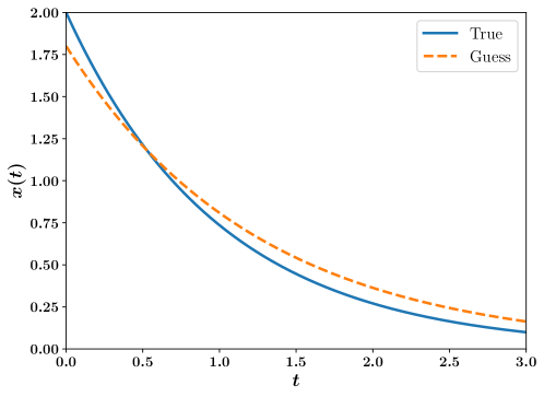
Figure 1: Solution of the decay model using the true and guess controls.

Synthetic observations are created from the true state with added noise of zero mean and a standard deviation $10\%$ of the model state at times when the observations are made. We follow the proposed methodology for placing the observation where the forward sensitivities attain their maximum values. For the considered exponential decay model, the forward sensitivities of the model predictions with respect to the control variables can be written as follows:

$$u(t)=e^{at},\quad v(t)=te^{at}x_{0}=tx(t).$$ (54)

With $a<0$, $u(t)=e^{-|a|t}$ attains the maximum at $t=0$ and $v(t)=te^{-|a|t}x$ attains the maximum at $t^{*}=\dfrac{1}{|a|}$. To avoid a zero value of $v(t)$, we avoid placing observations at $t=0$. Moreover, it can be verified from Eq. 34 that $|G|=0$ if $t_{1}=t_{2}$. Therefore, we can place the two observations at $t_{1}=\epsilon>0$ where $\epsilon$ is a small value (as opposed to having the observation coincide with the initial time) and $t_{2}=t^{*}=\dfrac{1}{|a|}$. In this case, it can be shown that $G$ is given by

$$G=e^{-2|a|\epsilon}\begin{bmatrix}1&\epsilon x_{0}\\ \epsilon x_{0}&\epsilon^{2}x_{0}^{2}\end{bmatrix}+e^{-2|a|t^{*}}\begin{bmatrix}1&t^{*}x_{0}\\ t^{*}x_{0}&t^{*2}x_{0}^{2}\end{bmatrix},$$ (55)

which is positive definite. The plots of forecast sensitivities to initial condition $x_{0}$ and decay parameter $a$ are shown in Fig. 2 for the true and guessed values of control $c$. In order to optimize the solution of the inverse problem, observation sites are chosen where the forecast sensitivities to control reach a maximum (i.e., $u^{2}(t)$ and $v^{2}(t)$ exhibit maxima). In particular, we place an observation at $t_{1}=k_{1}=\epsilon=0.1$ (to avoid singularity of the Gramian, G, in Eq. 34) and at $t_{2}=k_{2}=1.0$.

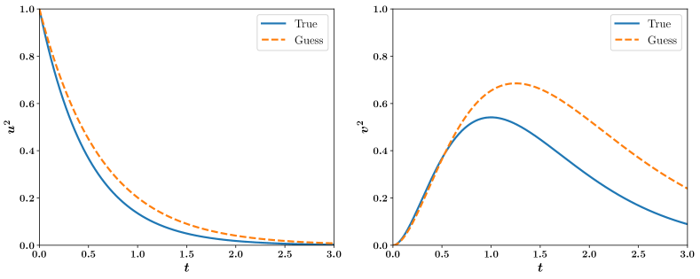
Figure 2: Model sensitivity with respect to (a) initial condition $x_{0}$ (left) and (b) the decay parameter $a$ (right).

The resulting cost function is displayed in Fig. 3 for different control values where the minimum value occurs around the true values of the control. Numerically, the search for the minimum can be made using Newton’s method, leading to optimal estimates of the control values as $c=(x_{0},a)=(1.7329,-0.7256)$.

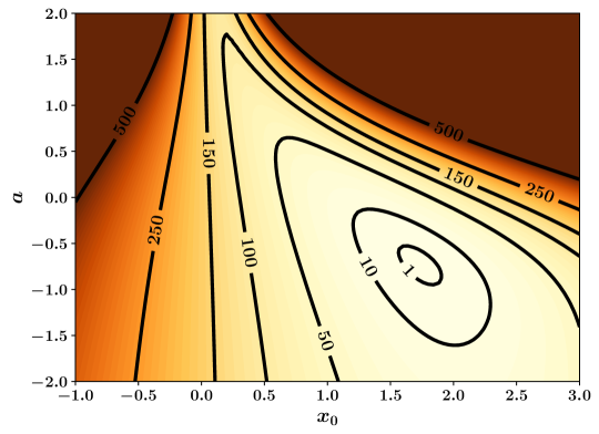
Figure 3: Cost function for exponential decay model.

Plots of sensitivity of the optimal control estimates with respect to observations (i.e., $y_{1}^{2}(t)$, $w_{1}^{2}(t)$, $y_{2}^{2}(t)$, and $w_{2}^{2}(t)$) are given in Fig. 4 through Fig. 7. Figure 4 shows the contour plot of $y_{1}^{2}(t)$ as well as the cross sections of this contour at the observation times (i.e., $t_{1}=0.1$ and $t_{2}=1.0$). Similar plots for $w_{1}^{2}(t)$ are covered in Fig. 5. It can be seen that maximum values of the sensitivity of the optimal estimate of $x_{0}$ with respect to the first observation occur when $t_{1}$ and $t_{2}$ are close to each other. For example, by selecting $t_{1}=0.1$, placing the second observation at earlier times (e.g., $t_{2}<0.5$) leads to very high sensitivity of the optimal estimate of $x_{0}$ and $a$ with respect to the first observation location. Thus, larger values of $t_{2}$ are to be sought to minimize $y_{1}^{2}$.

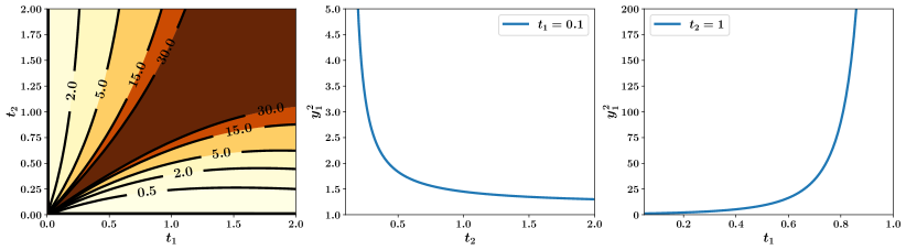
Figure 4: Sensitivity of the optimal estimates of the initial condition $x_{0}$ to the first observation $z_{1}$. Left: contour plot of $y_{1}^{2}(t)$ at different values of $t_{1}$ and $t_{2}$. Middle: $y_{1}^{2}(t)$ values at $t_{1}=0.1$ and different values of $t_{2}$. Right: $y_{1}^{2}(t)$ values at $t_{2}=1.0$ and different values of $t_{1}$. Note that minimum values of $y_{1}^{2}$ are obtained at $t_{1}=0.1$ and $t_{2}=1.0$.

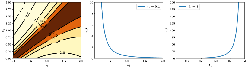
Figure 5: Sensitivity of the optimal estimates of the decay parameter $a$ to the first observation $z_{1}$. Left: contour plot of $w_{1}^{2}(t)$ at different values of $t_{1}$ and $t_{2}$. Middle: $y_{1}^{2}(t)$ values at $t_{1}=0.1$ and different values of $t_{2}$. Right: $w_{1}^{2}(t)$ values at $t_{2}=1.0$ and different values of $t_{1}$. Note that minimum values of $w_{1}^{2}$ are obtained at $t_{1}=0.1$ and $t_{2}=1.0$.

Likewise, Fig. 6 describes the properties of $y_{2}^{2}(t)$ and Fig. 7 displays properties of $w_{2}^{2}(t)$. As expected from the theory, the sensitivity of the optimal control estimates with respect to the observations exhibit minimum values at the two times where the observation sites were chosen. For example, by selecting $t_{1}=0.1$, $y_{2}^{2}$ and $w_{2}^{2}$ approach their minimum values at $t_{2}=1$. In a similar way, by selecting $t_{2}=1$, $y_{2}^{2}$ and $w_{2}^{2}$ are minimized by placing the first observation at very small values of $t_{1}$.

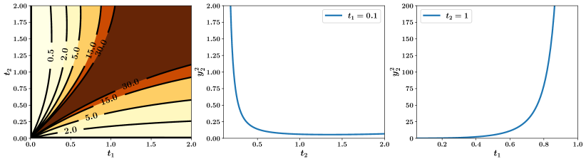
Figure 6: Sensitivity of the optimal estimates of the initial condition $x_{0}$ to the second observation $z_{2}$. Left: contour plot of $y_{2}^{2}(t)$ at different values of $t_{1}$ and $t_{2}$. Middle: $y_{2}^{2}(t)$ values at $t_{1}=0.1$ and different values of $t_{2}$. Right: $y_{1}^{2}(t)$ values at $t_{2}=1.0$ and different values of $t_{1}$. Note that minimum values of $y_{2}^{2}$ are obtained at $t_{1}=0.1$ and $t_{2}=1.0$.

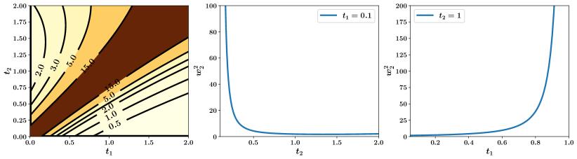
Figure 7: Sensitivity of the optimal estimates of the decay parameter $a$ to the second observation $z_{2}$. Left: contour plot of $w_{2}^{2}(t)$ at different values of $t_{1}$ and $t_{2}$. Middle: $y_{1}^{2}(t)$ values at $t_{1}=0.1$ and different values of $t_{2}$. Right: $w_{1}^{2}(t)$ values at $t_{2}=1.0$ and different values of $t_{1}$. Note that minimum values of $w_{2}^{2}$ are obtained at $t_{1}=0.1$ and $t_{2}=1.0$.

5.2 Nonlinear dynamics (scalar)

We extend our analysis and consider a system governed by nonlinear dynamics as follows:

$$\dot{x}=ax^{2},$$ (56)

where $x\in\mathbb{R}$ is the state variable and $a\in\mathbb{R}$ is the model parameter. It can be further shown that the solution of this system is given by $x(t)=\dfrac{x_{0}}{1-ax_{0}t}$. The true and guessed controls are defined as $\bar{c}=[\bar{x}_{0},\bar{a}]^{\mkern-1.5mu\mathsf{T}}=[2,-1]^{\mkern-1.5mu\mathsf{T}}$ and $c=[x_{0},a]^{\mkern-1.5mu\mathsf{T}}=[1.75,-0.75]^{\mkern-1.5mu\mathsf{T}}$, respectively. The dynamical evolution of the nonlinear decay system in response to the true and guess controls is shown in Fig. 8.

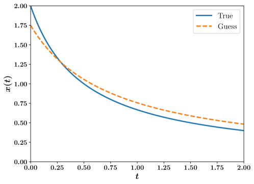
Figure 8: Solution of the nonlinear decay model using the true and guess controls.

The sensitivity of the model forecast with respect to the initial condition and model parameter can be written as follows:

$$u(t)=\dfrac{1}{(1-ax_{0}t)^{2}},\quad v(t)=\dfrac{x_{0}^{2}t}{(1-ax_{0}t)^{2}}.$$ (57)

The evolution of these sensitivities with time is depicted in Fig. 9. We note that similar figures can be obtained by solving Eq. 3 numerically, where $D_{f}(x)=2ax$ and $D_{f}^{a}(x)=x^{2}$.

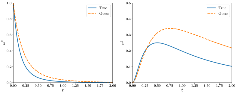
Figure 9: Model sensitivity with respect to (a) initial condition $x_{0}$ (left) and (b) the decay parameter $a$ (right) for $\dot{x}=ax^{2}$.

Although the maximum value of $u^{2}$ occurs at $t=0$, it corresponds to a zero value of $v^{2}$. Thus, we avoid placing observations at the initial time and we select $t_{1}=\epsilon=0.1>0$. Moreover, we select $t_{2}=0.5$ to maximize the value of $v^{2}$. We follow a twin experiment approach to generate synthetic observations by adding white Gaussian noise to the true system state (corresponding to the true controls). The resulting cost function is depicted in Fig. 10, where Newton’s method can be followed to obtain the optimal values of $x_{0}$ and $a$.

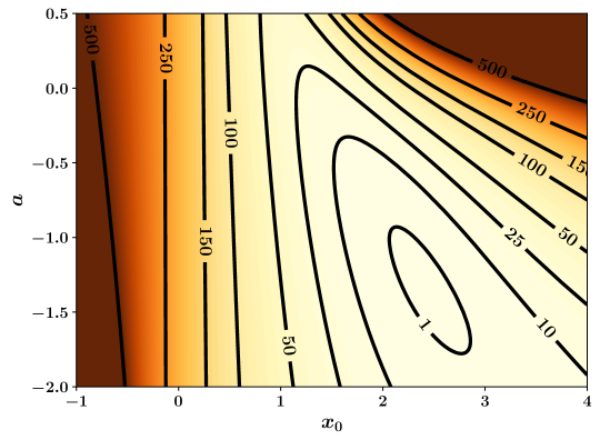
Figure 10: Cost function for nonlinear decay model: $\dot{x}=\alpha x^{2}$.

As highlighted before, we place the observations where the squares of the forward sensitivities of the model forecast with respect to the control are maximized. This guarantees that the observability Gramian is positive definite and subsequently keeps the adjoint gradient away from zero, which in turn accelerates the search for optimal estimates of the control. The second advantage of the proposed observation placement strategy is related to the robustness of the solution of the inverse problems against small perturbations to the collected measurement data. Figure 11 depicts the sensitivity of the optimal estimate of initial condition with respect to the first observation, considering a total of two observations at $t_{1}$ and $t_{2}$. From the contour plots of $y_{1}^{2}$, we see that collecting the two observations at close time instants results in higher sensitivity of the estimated initial condition to the measurement itself. Similar observations are obtained from Fig. 12 for $w_{1}^{2}$, where $w_{1}$ denotes the sensitivity of the optimal estimate of the model parameter with respect to the first observation. This is in agreement with the fact that highly correlated measurements do not add valuable information to the inversion problem. Moreover, from Eq. 34, when $t_{1}$ and $t_{2}$ coincide, the determinant of the observability Gramian vanishes, resulting in extreme values of the sensitivities $y_{i}$ and $w_{i}$ for $i=1,2$.

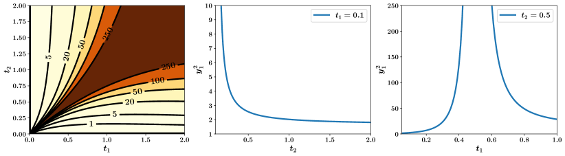
Figure 11: Sensitivity of the optimal estimates of the initial condition $x_{0}$ to the first observation $z_{1}$ for the nonlinear system $\dot{x}=\alpha x^{2}$. Left: contour plot of $y_{1}^{2}(t)$ at different values of $t_{1}$ and $t_{2}$. Middle: $y_{1}^{2}(t)$ values at $t_{1}=0.1$ and different values of $t_{2}$. Right: $y_{1}^{2}(t)$ values at $t_{2}=0.5$ and different values of $t_{1}$.

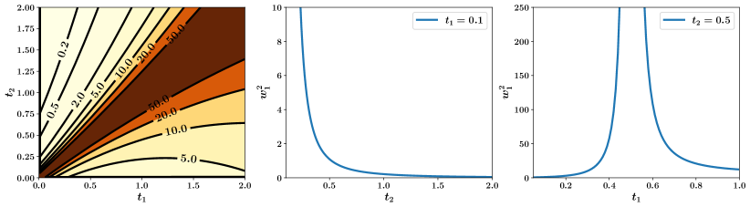
Figure 12: Sensitivity of the optimal estimates of the decay parameter $a$ to the first observation $z_{1}$ for the nonlinear system $\dot{x}=\alpha x^{2}$. Left: contour plot of $w_{1}^{2}(t)$ at different values of $t_{1}$ and $t_{2}$. Middle: $y_{1}^{2}(t)$ values at $t_{1}=0.1$ and different values of $t_{2}$. Right: $w_{1}^{2}(t)$ values at $t_{2}=0.5$ and different values of $t_{1}$.

Figures 13 and 14 display the sensitivity of the inferred initial condition and model parameter, respectively, to the second observation value at $t_{2}$. Similar to $y_{1}^{2}$ and $w_{1}^{2}$ plots, we see that maximum values of $y_{2}^{2}$ and $w_{2}^{2}$ occur when $t_{1}$ and $t_{2}$ are close to each other. In addition, looking at $y_{2}^{2}$ and $w_{2}^{2}$ values at $t_{1}=0.1$, it is clear that $y_{2}^{2}$ and $w_{2}^{2}$ exhibit very large values at small values of $t_{2}$, then decrease to attain their minima around $t_{2}=0.5$ before slightly increasing again at larger values of $t_{2}$. In a similar fashion, through an investigation of $y_{2}^{2}$ and $w_{2}^{2}$ at $t_{2}=0.5$ with varying $t_{1}$, we observe that maximum values occur when $t_{1}=t_{2}=0.5$. On the other hand, minimum values of the sensitivity of the control estimate with respect to the second measurement $z_{2}$ at $t_{2}=0.5$ occur when the first measurement is collected earlier at small values of $t_{1}$. The numerical investigations of the sensitivity of the inverse problem solution to the observation values and locations confirm that they are minimized when the observations are placed using the proposed forward sensitivity analysis. By placing the observations at points where the squares of the forward sensitivities of the forecast are maximized, we (1) control the shape of the cost function in such a way that flat patches (with zero gradients) are avoided, which improves the convergence characteristics of solving the inverse problem, and (2) guarantee that the sensitivities of the estimated control values (solution to the inverse problem) with respect to the measurement values are minimized, which enhances the robustness of the inversion framework against possible perturbations in the collected sensor data.

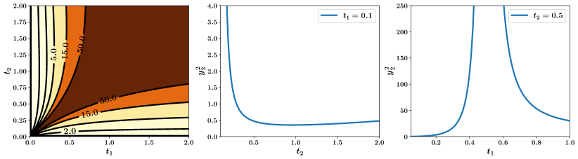
Figure 13: Sensitivity of the optimal estimates of the initial condition $x_{0}$ to the second observation $z_{2}$ for the nonlinear system $\dot{x}=\alpha x^{2}$. Left: contour plot of $y_{2}^{2}(t)$ at different values of $t_{1}$ and $t_{2}$. Middle: $y_{2}^{2}(t)$ values at $t_{1}=0.1$ and different values of $t_{2}$. Right: $y_{1}^{2}(t)$ values at $t_{2}=0.5$ and different values of $t_{1}$.

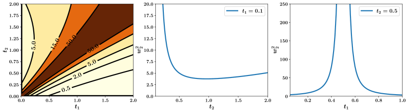
Figure 14: Sensitivity of the optimal estimates of the decay parameter $a$ to the second observation $z_{2}$ for the nonlinear system $\dot{x}=\alpha x^{2}$. Left: contour plot of $w_{2}^{2}(t)$ at different values of $t_{1}$ and $t_{2}$. Middle: $y_{1}^{2}(t)$ values at $t_{1}=0.1$ and different values of $t_{2}$. Right: $w_{1}^{2}(t)$ values at $t_{2}=0.5$ and different values of $t_{1}$.

5.3 1D Burgers problem

Our third test case is an advection shock problem governed by the 1D viscous Burgers equation as follows:

$$\dfrac{\partial u}{\partial t}+u\dfrac{\partial u}{\partial x}=\dfrac{1}{\text{Re}}\dfrac{\partial^{2}u}{\partial x^{2}},$$ (58)

where $u(x,t)$ is the velocity field and Re is the dimensionless Reynolds number, defined as the ratio of inertial effects to viscous effects. We first perform spatial discretization by defining the velocity field at $n$ discrete locations, equally spaced in the domain $L$. We apply a second-order centered finite difference scheme for the linear term and use the skew-symmetric formulation by Aref and Daripa’s scheme [54] for the nonlinear term as follows:

$$\dfrac{\partial u_{i}}{\partial t}=-\dfrac{1}{3}\dfrac{(u_{i+1}+u_{i-1}+u_{i})(u_{i+1}-u_{i-1})}{2\Delta x}+\dfrac{1}{\text{Re}}\dfrac{u_{i+1}-2u_{i}+u_{i-1}}{\Delta x^{2}},$$ (59)

where $\Delta x$ is the grid spacing, $\Delta x=x_{i+1}-x_{i}$. By arranging the velocity field in a column vector, Eq. 59 is equivalent to Eq. 35. We define a domain of length $L=1$ and enforce zero Dirichlet boundary conditions, $u(0,t)=u(1,t)=0$. A twin experiment is employed to generate observational data and assess the quality of the solution to inverse problems. In particular, the ground truth corresponds to $\text{Re}=500$ and the following initial condition [55]:

$$u(x,0)=\dfrac{x}{1+\exp{\left(\dfrac{\text{Re}}{16}\left(4x^{2}-1\right)\right)}},$$ (60)

while the background solution corresponds to a sinusoidal wave as $u(x,0)=\sin(2\pi x/L)$. Because it is unfeasible to track individual components of the forecast sensitivity matrices, we focus on the following two quantities:

$$I_{1}=\text{trace}\big{(}\mathbf{u}^{\mkern-1.5mu\mathsf{T}}\mathbf{u}\big{)},\qquad I_{2}=\dfrac{1}{2}\Bigg{(}\bigg{(}\text{trace}\big{(}\mathbf{u}^{\mkern-1.5mu\mathsf{T}}\mathbf{u}\big{)}\bigg{)}^{2}-\text{trace}\bigg{(}\big{(}\mathbf{u}^{\mkern-1.5mu\mathsf{T}}\mathbf{u}\big{)}^{2}\bigg{)}\Bigg{)}.$$ (61)

Figure 15 shows the time variation of $I_{1}$ and $I_{2}$ for the 1D Burgers problem. Both quantities attain their largest values near the initial time along with an additional bump around $t=0.35$.

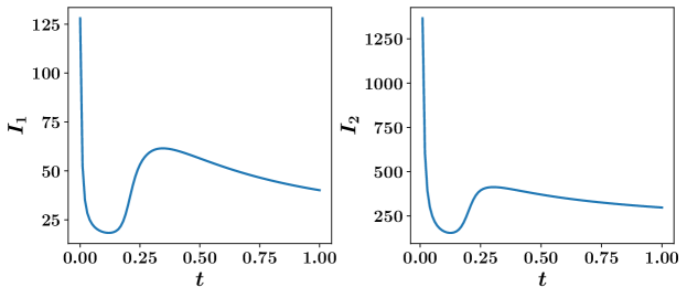
Figure 15: The first two invariants for the model forecast sensitivities with respect to the initial condition for the 1D viscous Burgers problem.

We empirically explore the advantages of the FSM-based observation placement strategy by considering different scenarios. The first two rows in Fig. 16 correspond to placing the observations by tracing the model forecast sensitivities. In particular, our first experiment corresponds to placing the observations near the initial time at $t=0.01$ and $t=0.05$. The second experiment corresponds to placing one observation at $t=0.01$ and another at $t=0.35$ near the second peak in Fig. 15. We test the quality of the inverse problem solution with different levels of measurement noise. Figure 16 demonstrates that the FSM placement strategy enables the accurate inference of the unknown initial condition even with large levels of noise. In this figure and the remaining discussion, we use standard terminology from data assimilation studies, where “background” refers to the estimated guess of unknown initial conditions and/or parameters. This estimate could be based on previous model predictions, historical data, or an intelligent guess. Thus, the background solution is the model forecast based on these supposedly inaccurate estimates. On the other hand, “analysis” refers to the solution of the inverse problem (e.g., for unknown initial conditions and/or parameters) after assimilating observation data. We highlight that we apply a truncated singular value decomposition as a regularization technique for solving the inverse problem. Our third experiment corresponds to arbitrarily placing the observations at $t=0.25$ and $t=0.50$ while we place them at $t=0.50$ and $t=1.0$ in our fourth experiment. We can see that both cases result in an inaccurate solution of the inverse problem. It is worth noting that this inaccuracy is in part due to the off-target background information (the sinusoidal wave). However, this exaggeration is intentional to show the benefits of the proposed placement strategy even in challenging situations. Finally, the predicted velocity fields are depicted in Fig. 17, where placing the observations closer to the maximum values of the forecast sensitivities yields improved results.

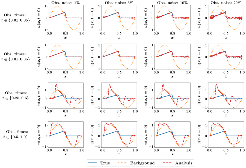
Figure 16: A comparison between inverse problem solutions (for initial conditions) at different observation placement times and varying levels of noise for the 1D viscous Burgers problem. Background refers to the guessed (inaccurate) initial conditions while the analysis refers to the solution of the inverse problem after observations have been assimilated.

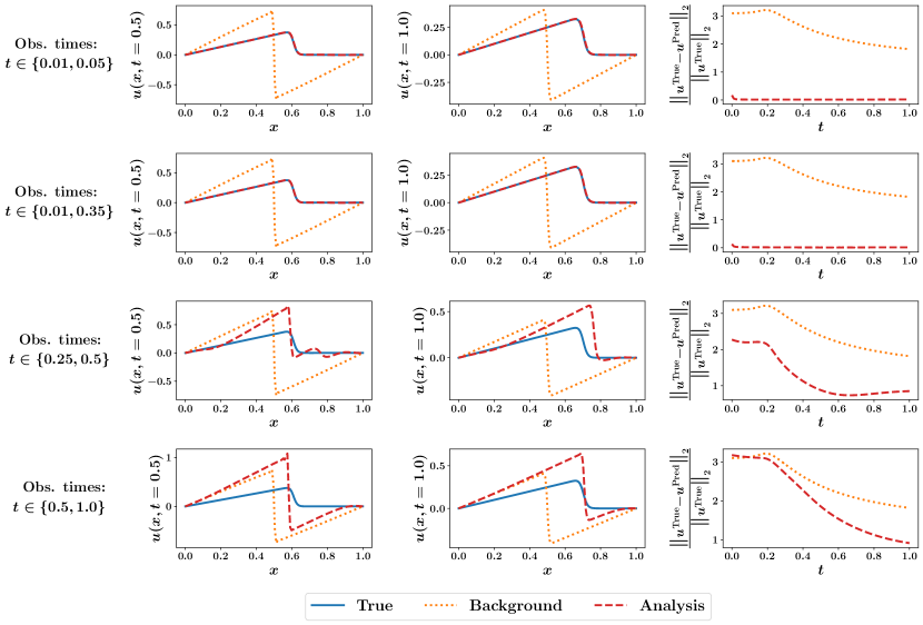
Figure 17: The predicted velocity field at $t=0.5$ (left) and $t=1.0$ (middle) for the 1D viscous Burgers problem with different observation placement times with $10\%$ measurement noise along with the relative $\ell_{2}$ error of the predicted velocity field at different times (right). Background solution refers to the forecast using the guessed (inaccurate) initial conditions while the analysis refers to the forecast after observations have been assimilated.

5.4 2D advection diffusion problem

Our last test case is the 2D advection diffusion equation as follows:

$$\dfrac{\partial u}{\partial t}+c_{x}\dfrac{\partial u}{\partial x}+c_{y}\dfrac{\partial u}{\partial y}=\nu\Big{(}\dfrac{\partial^{2}u}{\partial x^{2}}+\dfrac{\partial^{2}u}{\partial y^{2}}\Big{)}.$$ (62)

Equation 62 can be used to describe the evolution of the concentration of a substance under convection and diffusion effects, and the inversion of unknown initial conditions can be particularly important in the context of (contaminant) leak detection. Thus, variants of this test case have been used extensively in the literature of data assimilation and optimal experimental designs [56, 57, 58]. We use $c_{x}=c_{y}=0.5$ and $\nu=0.01$ and consider an initial condition of Gaussian distribution centered at $(x_{0},y_{0})$ as $u(x,y,0)=e^{-\frac{1}{\nu}\big{(}(x-x_{0})^{2}+(y-y_{0})^{2}\big{)}}$. The true field corresponds to $(x_{0},y_{0})=(0.25,0.25)$ while the background (guess) solution corresponds to $(x_{0},y_{0})=(0.5,0.5)$.

Figure 18 illustrates that the model forecast sensitivity with respect to the initial conditions exhibits maximum values near the initial time. In Fig. 19, we repeat the solution of the inverse problems whilst varying the times at which we place our observations. While it might not be possible in practice to place all observations near the initial time, Fig. 18 gives theoretical guidelines to prioritize observations at specific time instants over others. For instance, it is evident from Fig. 19 that placing observations at $t=0.5$ and $t=1.0$ (corresponding to minimum values of forecast sensitivities) produce erroneous initial conditions. On the other hand, collecting data at $t=0.1$ and $t=0.2$ (where the forward sensitivities are relatively larger) results in a better inference of the unknown initial condition. Finally, the predicted solution at $t=1$ is shown in Fig. 20 where observations are placed at $t=0.01$ and $t=0.05$.

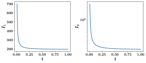
Figure 18: The first two invariants for the model forecast sensitivities with respect to initial conditions for the 2D advection diffusion problem.

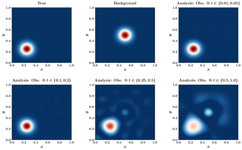
Figure 19: A comparison between inverse problem solutions (for initial conditions) at different observation placement times with $10\%$ measurement noise for the 2D advection diffusion problem. Background refers to the guessed (inaccurate) initial conditions while the analysis refers to the solution of the inverse problem after observations have been assimilated.

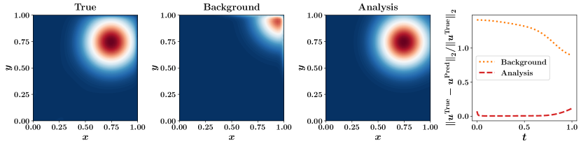
Figure 20: The predicted solution at $t=1$ for the 2D advection diffusion problem following the proposed observation placement strategy (with $10\%$ measurement noise) along with the relative $\ell_{2}$ error of the predicted velocity field at different times (right). Background solution refers to the forecast using the guessed (inaccurate) initial conditions while the analysis refers to the forecast after observations have been assimilated.

6 Conclusions

This paper systematically introduces a unified notion in the analysis and application of FSM to various questions related to forecast error correction using dynamic data assimilation [53]. We propose a strategy based on maximizing the square of the forward sensitivities, which guarantees efficient recovery of control variables and minimizes the sensitivity of optimal control estimates with respect to observations. First and foremost, the contribution of this paper can be better understood when compared with our ongoing efforts dedicated to the development of the FSM framework. In Lakshmivarahan and Lewis [52], we first proved the equivalence between FSM and the 4-D VAR method. In Lakshmivarahan et al. [24, 25] by relating the observability Gramian to the forward sensitivities, we derived an intrinsic expression for the adjoint sensitivity in terms of the observability Gramian. By exploiting the structure of the observability Gramian, we then derived a strategy to place observations where the squares of the forward sensitivities attain maximum values.

In this paper, we provide a detailed analysis of this observation placement strategy and show that it provides two crucial advantages in the context of inverse problems. First, we demonstrate that the FSM observation placement strategy avoids the occurrence of flat patches in the cost functional and improves the effectiveness of the minimization algorithm. Second, we also prove that it minimizes the sensitivity of the estimates (of the inverted quantities) with respect to the observations. The smallness of these quantitative measurements of the sensitivity of the estimates to observations supports determining observation sites using forward sensitivities. An advantage of the FSM analysis is that it does not require the adjoint code. However, computing the forward sensitivities is computationally demanding, but once done, we can solve two related problems. First, we can place the observations where the forward sensitivity attains a maximum value. Second, we can compute the optimal estimates of the control using FSM.

Appendix A – Proof of the second advantage of the FSM observation placement strategy: Scalar case

In this Appendix, we derive an intrinsic relation that exists between the sensitivities of the estimates of the control with respect to the observations, namely $y_{j}$ and $w_{j}$ for $1\leq j\leq 2$, and the forward sensitivities $u(k)$ and $v(k)$.

• Step 1: Derivatives of $x(t)$, $u(t)$, $v(t)$, and $D_{h}(x(t))$ with respect to the observation $z_{j}$ for $1\leq j\leq 2$ are given by

  $$\dfrac{\partial x(t)}{\partial z_{j}}=u(t)y_{j}+v(t)w_{j},\qquad\dfrac{\partial u(t)}{\partial z_{j}}=\dfrac{\partial u(t)}{\partial x_{0}}y_{j}+\dfrac{\partial u(t)}{\partial\alpha}w_{j},\qquad\dfrac{\partial v(t)}{\partial z_{j}}=\dfrac{\partial v(t)}{\partial x_{0}}y_{j}+\dfrac{\partial v(t)}{\partial\alpha}w_{j},$$ (63)

  $$\dfrac{\partial D_{h}(x(t))}{\partial z_{j}}=D_{h}^{(2)}(x(t))\dfrac{\partial x(t)}{\partial z_{j}},\qquad\text{where }D_{h}^{(2)}(x)=\dfrac{\partial^{2}h}{\partial x^{2}}\neq\left(\dfrac{\partial h}{\partial x}\right)^{2}.$$

• Step 2: From the definition of $e(t)$ in Eq. 9, we get

  $$\dfrac{\partial e(t)}{\partial z_{j}}=\delta_{tj}-D_{h}(x(t))\dfrac{\partial x(t)}{\partial z_{j}},$$ (64)

  where $\delta_{tj}$ is the Kronecker delta (i.e., $\delta_{tj}=1$ if $t=j$ and $\delta_{tj}=0$ otherwise).

• Step 3: Differentiating $H_{1j}$ in Eq. 28 with respect to $z_{p}$, we get the following:

  $$\left(\delta_{jp}-D_{h}(x(j))\dfrac{\partial x(j)}{\partial z_{p}}\right)D_{h}(x(j))u(j)+e(j)\dfrac{\partial D_{h}(x(j))}{\partial z_{p}}u(j)+e(j)D_{h}(x(j))\dfrac{\partial u(j)}{\partial z_{p}}=0.$$ (65)

• Step 4: Differentiating $H_{2j}$ in Eq. 29 with respect to $z_{p}$, we get the following:

  $$\left(\delta_{jp}-D_{h}(x(j))\dfrac{\partial x(j)}{\partial z_{p}}\right)D_{h}(x(j))v(j)+e(j)\dfrac{\partial D_{h}(x(j))}{\partial z_{p}}v(j)+e(j)D_{h}(x(j))\dfrac{\partial v(j)}{\partial z_{p}}=0.$$ (66)

• Step 5: When $x(t)$ is optimal, a little reflection reveals that $e(k)$ along the optimal path is small, and henceforth it is set to zero in Eqs. 65 and 66. Thus, the approximate expressions for $\dfrac{\partial H_{ij}}{\partial z_{p}}$ can be given as listed in Table 2.

  Table 2: Expressions for $\dfrac{\partial H_{ij}}{\partial z_{p}}$ for $i,j,p\in\{1,2\}$.

  		$j=1$	$j=2$
  $i=1$	$p=1$	$\left(1-D_{h}(1)\dfrac{\partial x(1)}{\partial z_{1}}\right)D_{h}(1)u(1)$	$-D_{h}^{2}(2)\dfrac{\partial x(2)}{\partial z_{1}}u(2)$
  	$p=2$	$-D_{h}^{2}(1)\dfrac{\partial x(1)}{\partial z_{2}}u(1)$	$\left(1-D_{h}(2)\dfrac{\partial x(2)}{\partial z_{2}}\right)D_{h}(2)u(2)$
  $i=2$	$p=1$	$\left(1-D_{h}(1)\dfrac{\partial x(1)}{\partial z_{1}}\right)D_{h}(1)v(1)$	$-D_{h}^{2}(2)\dfrac{\partial x(2)}{\partial z_{1}}v(2)$
  	$p=2$	$-D_{h}^{2}(1)\dfrac{\partial x(1)}{\partial z_{2}}v(1)$	$\left(1-D_{h}(2)\dfrac{\partial x(2)}{\partial z_{2}}\right)D_{h}(2)v(2)$

• Step 6: The optimality conditions (i.e., $\dfrac{\partial H_{i}}{\partial z_{p}}=\dfrac{\partial H_{i1}}{\partial z_{p}}+\dfrac{\partial H_{i2}}{\partial z_{p}}$) reduce to the following:

  $$D_{h}(1)u(1) =D_{h}^{2}(1)\dfrac{\partial x(1)}{\partial z_{1}}u(1)+D_{h}^{2}(2)\dfrac{\partial x(2)}{\partial z_{1}}u(2),$$ (67)

  $$D_{h}(2)u(2) =D_{h}^{2}(1)\dfrac{\partial x(1)}{\partial z_{2}}u(1)+D_{h}^{2}(2)\dfrac{\partial x(2)}{\partial z_{2}}u(2),$$ (68)

  $$D_{h}(1)v(1) =D_{h}^{2}(1)\dfrac{\partial x(1)}{\partial z_{1}}v(1)+D_{h}^{2}(2)\dfrac{\partial x(2)}{\partial z_{1}}v(2),$$ (69)

  $$D_{h}(2)v(2) =D_{h}^{2}(1)\dfrac{\partial x(1)}{\partial z_{2}}v(1)+D_{h}^{2}(2)\dfrac{\partial x(2)}{\partial z_{2}}v(2).$$ (70)

• Step 7: Substituting for $\dfrac{\partial x(t)}{\partial z_{j}}$ using Eq. 63 in Eqs. 67 and 69, we get

  $$D_{h}(1)u(1)=D_{h}^{2}(1)\left(u^{2}(1)+u(1)v(1)\right)y(1)+D_{h}^{2}(2)\left(u^{2}(2)+u(2)v(2)\right)w(1),$$ (71)

  $$D_{h}(1)v(1)=D_{h}^{2}(1)\left(u(1)v(1)+v^{2}(1)\right)y(1)+D_{h}^{2}(2)\left(u(2)v(2)+v^{2}(2)\right)w(1).$$ (72)

Referring to Eqs. 11 and 15, we define $F(i)=[u(i),v(i)]^{\mkern-1.5mu\mathsf{T}}\in\mathbb{R}^{2\times 1}$ and $G(i)=F^{\mkern-1.5mu\mathsf{T}}(i)D_{h}^{2}(i)F(i)\in\mathbb{R}^{2\times 2}$. Thus, Eq. 71 and Eq. 72 can be rewritten as

$$D_{h}(1)\begin{bmatrix}u(1)\\ v(1)\end{bmatrix}=G\begin{bmatrix}y_{1}\\ w_{1}\end{bmatrix},$$ (73)

where $G=G(1)+G(2)$. Therefore, $y_{1}$ and $w_{1}$ can be obtained as

$$\begin{bmatrix}y_{1}\\ w_{1}\end{bmatrix}=G^{-1}D_{h}(1)\begin{bmatrix}u(1)\\ v(1)\end{bmatrix}.$$ (74)

Similarly, from Eqs. 68 and 70 and using the same procedure, we get

$$\begin{bmatrix}y_{2}\\ w_{2}\end{bmatrix}=G^{-1}D_{h}(2)\begin{bmatrix}u(2)\\ v(2)\end{bmatrix}.$$ (75)

Appendix B – Linear independence of the forward sensitivities of the model forecast at different times with respect to the control

The discrete-time version of the model given in Eq. 1 can be written as:

$$x_{k+1}=M(x_{k},\alpha),$$ (76)

where $M:\mathbb{R}\times\mathbb{R}\to\mathbb{R}$ defines the one-time step mapping defined by applying a temporal integration scheme. Equation 3 for the dynamics of $u(t)$ and $v(t)$ can be rewritten as follows:

$$u_{k+1} =D_{M}(k)u_{k},\quad u_{0}=1,$$ (77)

$$v_{k+1} =D_{M}(k)v_{k}+D_{M}^{\alpha}(x_{k}),\quad v_{0}=0,$$

where

$$D_{M}(k)=\dfrac{\partial M}{\partial x}\bigg{|}_{x=x_{k}},\quad\text{and}\quad D_{M}^{\alpha}(k)=\dfrac{\partial M}{\partial\alpha}\bigg{|}_{x=x_{k}}.$$ (78)

For simplicity of notation, let $a_{k}:=D_{M}(k)$ and $b_{k}:=D_{M}^{\alpha}(k)$. Thus, the sequence of $u_{k}$ can be a written as follows:

$$u_{k} =a_{k-1}a_{k-2}\dots a_{1}a_{0},\qquad\text{for }\quad k\geq 1.$$ (79)

Similarly, the sequence of $v_{k}$ can be expanded as follows:

$$v_{k} =(a_{k-1}a_{k-2}\dots a_{1}b_{0})+(a_{k-1}a_{k-2}\dots a_{2}b_{1})+(a_{k-1}a_{k-2}\dots a_{3}b_{2})+\dots$$ (80)

$$+(a_{k-1}a_{k-2}b_{k-3})+(a_{k-1}b_{k-2})+(b_{k-1}),\qquad\text{for }\quad k\geq 1.$$

For the Gramian matrix $G$ in Eq. 33 to be singular (i.e., the determinant in Eq. 34 equals zero), the vectors $[u_{1},u_{2}]^{\mkern-1.5mu\mathsf{T}}$ and $[v_{1},v_{2}]^{\mkern-1.5mu\mathsf{T}}$ ought to be linearly dependent. In what follows, we show that this situation cannot happen. For the vectors $[u_{1},u_{2}]^{\mkern-1.5mu\mathsf{T}}$ and $[v_{1},v_{2}]^{\mkern-1.5mu\mathsf{T}}$ to be linearly dependent, we get $u_{k}=Cv_{k}$ for all $k$ where $C$ is a non-zero constant, then we can write the following:

$$u_{1} =Cv_{1}\Longleftrightarrow a_{0}=Cb_{0},$$ (81)

$$u_{2} =Cv_{2}\Longleftrightarrow a_{1}a_{0}=Ca_{1}b_{0}+Cb_{1}.$$ (82)

Because $a_{0}=Cb_{0}$, Eq. 82 can be rewritten as $a_{1}a_{0}=a_{1}a_{0}+Cb_{1}$, leading to $b_{1}=0$. Similarly,

$$u_{3} =Cv_{3}\Longleftrightarrow a_{2}a_{1}a_{0}=Ca_{2}a_{1}b_{0}+Ca_{2}b_{1}+Cb_{2}.$$ (83)

With $a_{0}=Cb_{0}$ and $b_{1}=0$, we also get $b_{2}=0$. Following the same procedure, this leads to $b_{k}=D_{M}^{\alpha}(k)=0$ for all $k\neq 0$. In other words, this implies that the sensitivity of the model $M$ with respect to the parameter $\alpha$ equals zero along the trajectory except at $t=0$. However, this cannot be the case because a model cannot be sensitive to its parameters at $t=0$ and not sensitive at other times. Therefore, the vectors of $u_{k}$ and $v_{k}$ cannot be linearly dependent, and the proposed observation placement strategy thus does not lead to a singular observability Gramian.

Data Availability

The data that support the findings of this study are available within the article.

References

- [1] A Tarantola. Inverse problem theory. Elsevier, New York, 1987.
- [2] Eugenia Kalnay. Atmospheric modeling, data assimilation and predictability. Cambridge University Press, 2003.
- [3] Jari Kaipio and Erkki Somersalo. Statistical and computational inverse problems, volume 160. Springer, Berlin, 2006.
- [4] John M Lewis, Sivaramakrishnan Lakshmivarahan, and Sudarshan Dhall. Dynamic data assimilation: a least squares approach, volume 104. Cambridge University Press, Cambridge, 2006.
- [5] George Biros, Omar Ghattas, Matthias Heinkenschloss, David Keyes, Bani Mallick, Luis Tenorio, Bart van Bloemen Waanders, Karen Willcox, Youssef Marzouk, and Lorenz Biegler. Large-scale inverse problems and quantification of uncertainty. John Wiley & Sons, 2011.
- [6] Christopher A Edwards, Andrew M Moore, Ibrahim Hoteit, and Bruce D Cornuelle. Regional ocean data assimilation. Annual Review of Marine Science, 7:21–42, 2015.
- [7] Mark Asch, Marc Bocquet, and Maëlle Nodet. Data assimilation: methods, algorithms, and applications. SIAM, 2016.
- [8] Andreas Vieli, Antony J Payne, Zhijun Du, and Andrew Shepherd. Numerical modelling and data assimilation of the larsen b ice shelf, antarctic peninsula. Philosophical Transactions of the Royal Society A: Mathematical, Physical and Engineering Sciences, 364(1844):1815–1839, 2006.
- [9] Peter L Houtekamer and Fuqing Zhang. Review of the ensemble kalman filter for atmospheric data assimilation. Monthly Weather Review, 144(12):4489–4532, 2016.
- [10] RN Bannister. A review of operational methods of variational and ensemble-variational data assimilation. Quarterly Journal of the Royal Meteorological Society, 143(703):607–633, 2017.
- [11] Alberto Carrassi, Marc Bocquet, Laurent Bertino, and Geir Evensen. Data assimilation in the geosciences: An overview of methods, issues, and perspectives. Wiley Interdisciplinary Reviews: Climate Change, 9(5):e535, 2018.
- [12] AJ Geer. Learning earth system models from observations: machine learning or data assimilation? Philosophical Transactions of the Royal Society A, 379(2194):20200089, 2021.
- [13] Julien Brajard, Alberto Carrassi, Marc Bocquet, and Laurent Bertino. Combining data assimilation and machine learning to infer unresolved scale parametrization. Philosophical Transactions of the Royal Society A, 379(2194):20200086, 2021.
- [14] Rudolf E Kalman. On the general theory of control systems. In Proceedings First International Conference on Automatic Control Congress, Moscow, USSR, pages 481–492, 1960.
- [15] John L Casti. Nonlinear systems theory. Academic Press, New York, 1985.
- [16] Alberto Isidori. Nonlinear control systems. Springer, Berlin, 1985.
- [17] Richard Bellman. Stability of differential equations. McGraw Hill, New York, 1953.
- [18] RG Brown. Not just observable, but how observable. In Proceedings of the 1966 National Electronics Conference, Volume 22, Chicago, IL, pages 709–714, 1966.
- [19] Wei Kang and Liang Xu. A quantitative measure of observability and controllability. In Proceedings of the 48h IEEE Conference on Decision and Control, Shanghai, China, pages 6413–6418, 2009.
- [20] Wei Kang and Liang Xu. Optimal placement of mobile sensors for data assimilations. Tellus A: Dynamic Meteorology and Oceanography, 64(1):17133, 2012.
- [21] Sarah King, Wei Kang, and Liang Xu. Observability for optimal sensor locations in data assimilation. International Journal of Dynamics and Control, 3(4):416–424, 2015.
- [22] François-Xavier Le Dimet and Olivier Talagrand. Variational algorithms for analysis and assimilation of meteorological observations: theoretical aspects. Tellus A: Dynamic Meteorology and Oceanography, 38(2):97–110, 1986.
- [23] Tilo Ochotta, Christoph Gebhardt, Dietmar Saupe, and Werner Wergen. Adaptive thinning of atmospheric observations in data assimilation with vector quantization and filtering methods. Quarterly Journal of the Royal Meteorological Society, 131(613):3427–3437, 2005.
- [24] S Lakshmivarahan, John M Lewis, and Junjun Hu. On controlling the shape of the cost functional in dynamic data assimilation: guidelines for placement of observations and application to Saltzman’s model of convection. Journal of the Atmospheric Sciences, 77(8):2969–2989, 2020.
- [25] S Lakshmivarahan, John M Lewis, and Sai Kiran Reddy Maryada. Observability Gramian and its role in the placement of observations in dynamic data assimilation. In Data Assimilation for Atmospheric, Oceanic and Hydrologic Applications (Vol. IV), pages 215–257. Springer, 2022.
- [26] John M Lewis, S Lakshmivarahan, Junjun Hu, and Robert Rabin. Placement of observations to correct return-flow forecasts. Electronic Journal of Severe Storms Meteorology, 15:1––20, 2020.
- [27] John M Lewis, S Lakshmivarahan, and Sai Kiran R Maryada. Placement of observations for variational data assimilation: application to Burgers’ equation and Seiche phenomenon. In Data Assimilation for Atmospheric, Oceanic and Hydrologic Applications (Vol. IV), pages 259–275. Springer, 2022.
- [28] Shady E Ahmed, Kinjal Bhar, Omer San, and Adil Rasheed. Forward sensitivity approach for estimating eddy viscosity closures in nonlinear model reduction. Physical Review E, 102(4):043302, 2020.
- [29] Shady E Ahmed, Omer San, and Sivaramakrishnan Lakshmivarahan. Forward sensitivity analysis of the FitzHugh–Nagumo system: Parameter estimation. In Advances in Nonlinear Dynamics, pages 93–103. Springer, 2022.
- [30] Wayne A Fuller. Introduction to statistical time series. Wiley, New York, 1976.
- [31] Peter J Brockwell and Richard A Davis. Time series: theory and methods (second edition). Springer, New York, 2006.
- [32] G A Seber and Wild C J. Nonlinear regression. Wiley Intersciences, New York, 1988.
- [33] A R Gallant. Nonlinear statistical models. Wiley, New York, 1987.
- [34] Ror Bellman and Karl Johan Åström. On structural identifiability. Mathematical Biosciences, 7(3-4):329–339, 1970.
- [35] Lennart Ljung. System identification. Prentice Hall, Englewood Cliff, NJ, 1999.
- [36] Kumpati S Narendra and Anuradha M Annaswamy. Stable adaptive systems. Prentice Hall, Englewood Cliff, NJ, 1989.
- [37] Alejandro F Villaverde. Observability and structural identifiability of nonlinear biological systems. Complexity, 2019:8497093, 2019.
- [38] Dariusz Ucinski. Optimal measurement methods for distributed parameter system identification. CRC Press, Baton Rouge, 2004.
- [39] J E Alaña. Optimal measurement locations for parameter estimation of non linear distributed parameter systems. Brazilian Journal of Chemical Engineering, 27:627–642, 2010.
- [40] T H Christopher and A R Fathalla. Sensitivity analysis of parameters in modelling with delay-differential equations. Manchester Center for Computational Mathematics, Numerical Analysis Reports, report no. 349, The University of Manchester, England, pages 180–199, 1999.
- [41] Dan G Cacuci. Sensitivity & uncertainty analysis, volume I: theory, volume 1. CRC Press, Boca Raton, 2003.
- [42] Dan G Cacuci, Mihaela Ionescu-Bujor, and Ionel Michael Navon. Sensitivity and uncertainty analysis, volume II: applications to large-scale systems, volume 2. CRC Press, Boca Raton, 2005.
- [43] Nancy L Baker and Roger Daley. Observation and background adjoint sensitivity in the adaptive observation-targeting problem. Quarterly Journal of the Royal Meteorological Society, 126(565):1431–1454, 2000.
- [44] Rolf H Langland and Nancy L Baker. Estimation of observation impact using the NRL atmospheric variational data assimilation adjoint system. Tellus A: Dynamic Meteorology and Oceanography, 56(3):189–201, 2004.
- [45] Dacian N Daescu. On the sensitivity equations of four-dimensional variational (4D-Var) data assimilation. Monthly Weather Review, 136(8):3050–3065, 2008.
- [46] Carla Cardinali. Monitoring the observation impact on the short-range forecast. Quarterly Journal of the Royal Meteorological Society, 135(638):239–250, 2009.
- [47] Ronald Gelaro and Yanqiu Zhu. Examination of observation impacts derived from observing system experiments (OSEs) and adjoint models. Tellus A: Dynamic Meteorology and Oceanography, 61(2):179–193, 2009.
- [48] Sharanya J Majumdar. A review of targeted observations. Bulletin of the American Meteorological Society, 97(12):2287–2303, 2016.
- [49] Brian Ancell and Gregory J Hakim. Comparing adjoint-and ensemble-sensitivity analysis with applications to observation targeting. Monthly Weather Review, 135(12):4117–4134, 2007.
- [50] Junjie Liu and Eugenia Kalnay. Estimating observation impact without adjoint model in an ensemble Kalman filter. Quarterly Journal of the Royal Meteorological Society, 134(634):1327–1335, 2008.
- [51] Vladimir I Arnold. Ordinary differential equations. Springer Science & Business Media, New York, 1992.
- [52] S Lakshmivarahan and John M Lewis. Forward sensitivity approach to dynamic data assimilation. Advances in Meteorology, 2010, 2010.
- [53] Sivaramakrishnan Lakshmivarahan, John M Lewis, and Rafal Jabrzemski. Forecast error correction using dynamic data assimilation. Springer, New York, 2017.
- [54] H Aref and PK Daripa. Note on finite difference approximations to Burgers’ equation. SIAM Journal on Scientific and Statistical Computing, 5(4):856–864, 1984.
- [55] Shady E Ahmed, Omer San, Adil Rasheed, and Traian Iliescu. A long short-term memory embedding for hybrid uplifted reduced order models. Physica D: Nonlinear Phenomena, 409:132471, 2020.
- [56] Noei Petra and Georg Stadler. Model variational inverse problems governed by partial differential equations. Technical report, Texas University at Austin Institute for Computational Engineering and Sciences, 2011.
- [57] Ahmed Attia, Sven Leyffer, and Todd S Munson. Stochastic learning approach for binary optimization: Application to Bayesian optimal design of experiments. SIAM Journal on Scientific Computing, 44(2):B395–B427, 2022.
- [58] Ahmed Attia and Shady E Ahmed. Pyoed: An extensible suite for data assimilation and model-constrained optimal design of experiments. arXiv preprint arXiv:2301.08336, 2023.