Refermionized theory of the edge modes of a fractional quantum Hall cloud

Abstract

Making use of refermionization techniques, we map the nonlinear chiral Luttinger liquid model of the edge modes of a spatially confined fractional quantum Hall cloud developed in our recent work [Phys. Rev. A 107, 033320 (2023)] onto a one-dimensional system of massive and interacting chiral fermions, whose mass and interactions are set by the filling factor of the quantum Hall fluid and the shape of the external anharmonic confining potential at the position of the edge. As an example of the predictive power of the refermionized theory, we report a detailed study of the dynamic structure factor and of the spectral function of a fractional quantum Hall cloud. Among other features, our refermionized theory provides a physical understanding of the effective decay of the edge excitations and of the universal power-law exponents at the thresholds of the dynamic structure factor. The quantitative accuracy of the refermionized theory is validated against full two-dimensional calculation based on a combination of exact diagonalization and Monte-Carlo sampling.

I Introduction

The fractional quantum Hall (FQH) effect is among the most fascinating concepts of modern quantum condensed matter physics Jain (2007); Prange et al. (2012), being a prototypical example of strongly correlated and incompressible quantum liquid exhibiting topological order Wen (2019). Such a state of matter was originally observed more than $40$ years ago in semiconductor hetero-structures hosting a two-dimensional electron gas subject to a strong perpendicular magnetic fields Tsui et al. (1982). Still now, it keeps attracting a strong attention due to its rich emergent physics, such as fractionally charged excitations Laughlin (1983); Tsui et al. (1982) with fractional Arovas et al. (1984) or even non-Abelian Nayak et al. (2008) exchange statistics, and gapless edge modes chirally propagating along the one-dimensional edge of the system Wen (1990a, b, 1991a, 1995, 1992); Chang (2003). Over the years, these latter modes have been a powerful probe of the system, providing evidence of the topological order of the bulk Wen (1995) via the observation of fractional charge in shot-noise experiments de-Picciotto et al. (1997) and of non-trivial power-law exponents in the $I$-$V$ characteristic of tunneling junctions Chang et al. (1996); Chang (2003), via thermal Hall conductance measurements Banerjee et al. (2018); Aharon Melcer et al. (2023), and, more recently, via direct measurements of the exchange statistics of the bulk quasiparticles Nakamura et al. (2020); Bartolomei et al. (2020). All these features are theoretically captured by a simple one-dimensional model, the chiral Luttinger liquid ($\chi$LL) theory Wen (1995), which provides an accurate description of the edge dynamics in the long-wavelength, low-energy, weak excitation limit.

While the FQH was originally observed in two-dimensional electron systems, a strong experimental attention is currently being devoted to the possibility of realizing FQH states in synthetic quantum matter systems, such as gases of ultra-cold atoms under synthetic magnetic fields Cooper (2008); Bloch et al. (2008); Cooper et al. (2019); Goldman et al. (2014) or fluids of strongly interacting photons in nonlinear topological photonics devices Carusotto et al. (2020); Carusotto and Ciuti (2013); Ozawa et al. (2019). Important experimental steps in this direction have been recently reported in both atomic Gemelke et al. (2010); Fletcher et al. (2021); Tai et al. (2017); Léonard et al. (2022) and photonic systems Schine et al. (2016); Clark et al. (2020); Roushan et al. (2017). These setups are very interesting not only because they would allow for the realization of novel FQH states of bosonic particles, but also because they typically offer more flexibility in the control of the system parameters as well as a wider variety of experimental tools as compared to the traditional transport and optical probes of electronic systems. In particular, while the generation and diagnostics of neutral edge excitations in electronic systems requires ultrafast tools that are presently being developed with state-of-the-art electronic and optical technologies Kamiyama et al. (2022); Ashoori et al. (1992), arbitrary space- and time-dependent potentials Gauthier et al. (2016) can be straightforwardly applied to synthetic systems and high-resolution detection tools at the single-particle level are available Gross and Bakr (2021).

With an eye to these on-going experimental developments, we are carrying out a long-term project devoted to the study of the quantum dynamics of a FQH edge beyond the $\chi$LL description. As a first step, in Nardin and Carusotto (2020) we investigated the linear and nonlinear dynamics of the edge of an Integer Quantum Hall (IQH) fluid. In the following work Nardin and Carusotto (2023), we extended the study to anharmonically trapped FQH clouds: based on the outcome of numerical calculations of the dynamics of two-dimensional FQH fluid, carried out via a novel combination of exact diagonalization with a Monte-Carlo sampling of the matrix elements, we highlighted novel features such as a sizable group velocity dispersion and nonlinear effects for the edge modes. This allowed us to develop a generalized nonlinear chiral Luttinger liquid (NL-$\chi$LL) theory able to quantitatively reproduce the numerical predictions.

In this work, we make a further step forward in this long-haul program by showing how the NL-$\chi$LL theory introduced in Nardin and Carusotto (2023) can be mapped onto a model of one-dimensional interacting chiral fermions. This allows to use techniques originally developed for Tomonaga-Luttinger liquids to shine qualitative and quantitative light on crucial features of the edge dynamics such as the broadening of the dynamic structure factor (DSF) and the spectral function (SF) of the FQH fluid, the appearance of universal power law exponents at spectral edges, and the fine structure of the microscopic eigenstates.

The structure of the article is the following. In Sec. II we describe the physical system under investigation and we briefly review the NL-$\chi$LL description we introduced in Nardin and Carusotto (2023). In Sec. III we present the reformulation of the problem in terms of a one-dimensional Tomonaga-Luttinger liquid model of massive and interacting chiral fermions. In Sec.IV we make use of the refermionized model to shine physical light on the predictions of the NL-$\chi$LL model and of the full 2D numerical calculations. Conclusions are finally given in section V.

II The physical system and the nonlinear chiral Luttinger liquid description

We consider a model of $N$ quantum particles of mass $m$ moving within a continuous two-dimensional plane, displaying short-range repulsive interactions, and subject to a uniform magnetic field $B$ orthogonal to the plane. As usual, the single-particle states in a uniform $B$ organize in highly degenerate and uniformly separated Landau levels: in what follows, energies are measured in units of the cyclotron splitting between Landau levels $\hbar\omega_{c}=\hbar\,qB/m$ and lengths in units of the magnetic length $\ell_{B}=\sqrt{\hbar/m\omega_{c}}$. Here $q$ is the charge of the particles. In the case of synthetic quantum matter, $qB$ is determined by the particular realization of the artificial gauge field. For example, in the case of rapidly rotating neutral atomsCooper (2008), $qB=2m\Omega_{r}$, $\Omega_{r}$ being the rotation frequency. We also adopt the usual complex-valued shorthand $z=x+iy$.

Two-body interactions lift the macroscopic degeneracy of Landau levels and lead to the formation of highly-correlated incompressible ground states. The simplest examples of such states are the celebrated Laughlin states Laughlin (1983); Halperin and Jain (2020)

$$\Psi_{L}(\left\{z_{i}\right\})=\prod_{i<j}(z_{i}-z_{j})^{1/\nu}\,\exp\left(-\frac{1}{4}\sum_{i}\left|z_{i}\right|^{2}\right),$$ (1)

which entirely sit within the lowest Landau level. While the Laughlin state at filling $\nu=1/2$ is the exact ground state for contact-interacting bosons Wilkin et al. (1998), other $\nu\neq 1/2$ Laughlin states are the exact ground state of certain bosonic or fermionic toy model Hamiltonians Haldane (1983); Trugman and Kivelson (1985); Simon et al. (2007a, b) and turn out to be excellent approximations of the ground state of more realistic problems. In the presence of a spatial in-plane confinement, the bulk of the FQH fluid maintains its incompressible nature, the ground state being separated by a finite energy gap from excited states, while the boundary hosts one-dimensional gapless chiral edge excitations Wen (1991a).

In this work, we focus our attention on the edge excitations of a FQH fluid, with a particular attention to the $\nu=1/2$ Laughlin state which is most relevant for cold bosonic matter subject to a strong synthetic magnetic field. These excitations correspond to chirally-propagating surface deformations of the incompressible cloud and, in the long-wavelength, low-energy, weak excitation limit, are accurately described by the $\chi$LL model Wen (1995, 1992); Chang (2003); Cazalilla (2003). On the other hand, the incompressible bulk only hosts gapped excitations, namely charged quasihole and quasielectrons Laughlin (1983) and neutral magneto-roton-like density excitations Girvin et al. (1986a). The magnitude of the many-body (or Laughlin) energy gap separating them from the ground state is set by the interparticle interactions.

In our previous work Nardin and Carusotto (2023) we considered a FQH cloud confined by a generic weakly anharmonic trap potential

$$V_{\text{conf}}(r)=\lambda r^{\delta}.$$ (2)

Under the assumption of a shallow trap and of moderate excitation strength, mixing with states above the many-body energy gap can be neglected and the dynamics is confined to the subspace of many-body wavefunctions obtained by multiplying the Laughlin wavefunction by holomorphic symmetric polynomials $P_{\alpha}\left(\left\{z_{i}\right\}\right)$ of the particle coordinates Stone (1990); Wen (1995); Halperin and Jain (2020),

$$\Psi_{\alpha}(\left\{z_{i}\right\})=P_{\alpha}\left(\left\{z_{i}\right\}\right)\,\Psi_{L}(\left\{z_{i}\right\}).$$ (3)

As long as we consider polynomials $P_{\alpha}$ of degree much smaller than the number of particles, these wavefunctions describe charge neutral excitations of the edge.

The temporal dynamics of the cloud was simulated by restricting to the class of states (3), evaluating the matrix elements by Monte Carlo sampling of the wavefunctions, and then performing the time-evolution on the restricted Hamiltonian with standard numerical techniques. The result of these full 2D numerical calculations was used to inspect the linear and non-linear dynamics of the edge modes in response to a spatially-dependent and pulsed excitation. This allowed us to identify new features of the dynamics beyond the standard $\chi$LL theory and, in particular, we showed that the low-energy, long-wavelength, weak-excitation physics of the FQH edge is successfully captured by a NL-$\chi$LL Hamiltonian of the form

$$\hat{H}=\int d\theta\left(\pi\,\frac{\Omega}{\nu}\,\hat{\rho}^{2}+\frac{c}{\nu^{2}}\,\frac{2\pi^{2}}{3}\,\hat{\rho}^{3}-\pi\frac{\beta_{\nu}}{\nu}\frac{c}{R_{cl}}\,\left(\partial_{\theta}\hat{\rho}\right)^{2}\right)$$ (4)

where the edge-density operators $\hat{\rho}$ obey the standard bosonic commutation relations Wen (1995)

$$[\hat{\rho}(\theta),\hat{\rho}(\theta^{\prime})]=-i\frac{\nu}{2\pi}\partial_{\theta}\delta(\theta-\theta^{\prime}).$$ (5)

of a $\chi$LL. In addition to this, the Hamiltonian Eq. (4) includes boson-boson interactions proportional to $\hat{\rho}^{3}$ and a surface-tension-like term proportional to $(\partial_{\theta}\hat{\rho})^{2}$, which causes a modification to the dispersion of linear waves. The parameter $\beta_{\nu}$ is a filling-dependent constant characteristic of Laughlin FQH states. From the microscopic calculations we performed it turns out to be approximately equal to $\beta_{\nu}\simeq\frac{\pi}{8}\frac{1-\nu}{\nu}$: while no solid theoretical explanation is yet available for this remarkably simple form, we conjecture that it may be justified by relating it to the viscosity of quantum Hall fluids Avron et al. (1995) and the gapped magneto-roton excitations of the bulk Girvin et al. (1986b).

The quantitative agreement of the NL-$\chi$LL theory with the full 2D numerical calculation is all the way more surprising given that it is a straightforward generalization of Wen’s $\chi$LL theory that, for a given topological state of filling factor $\nu$, only involves two non-universal parameters $\Omega$ and $c$ characterizing the confinement potential at the position of the cloud’s edge. These parameters physically correspond to the angular velocity of the edge modes

$$\Omega=R_{cl}^{-1}\partial_{r}V_{\text{conf}}|_{R_{cl}}=\lambda\,\delta\,R_{cl}^{\delta-2},$$ (6)

i.e. the force exerted by the confinement potential [Eq. (2)] at the classical radius $R_{cl}=\sqrt{2N/\nu}$ of the cloud, and to the radial gradient

$$c=R_{cl}^{-1}\partial_{r}\Omega|_{R_{cl}}=\lambda\,\delta(\delta-2)\,R_{cl}^{\delta-4}$$ (7)

of this force. In this work, we will restrict our attention to the case of positive-curvature confinement potentials with $c>0$. The different behaviours that occur for other forms of the potential will be explored in a forthcoming work.

In view of following developments, it is useful to note how the evolution of the edge-density operator under the NL-$\chi$LL Hamiltonian is the quantum analog of a Korteweg-de Vries equation of classical fluid dynamics

$$\partial_{t}\hat{\rho}=i[\hat{H},\hat{\rho}]=-\Omega\partial_{\theta}\hat{\rho}-\frac{\pi c}{\nu}\,\partial_{\theta}\hat{\rho}^{2}-\alpha\partial_{\theta}^{3}\hat{\rho}.$$ (8)

For the sake of completeness, it is worth noting that non-universal corrections to the $\chi$LL Hamiltonian analogous to Eq.(4) have been investigated also in the different context of reconstructed edges Yang (2003). Here, however, the non-trivial dispersion was the result of a gradient expansion of the non-local Coulomb interaction between electrons rather than an intrinsic property of strongly correlated FQH liquids with short-range interactions. Finally, a summary of all possible irrelevant perturbations to the $\chi$LL Hamiltonian allowed by symmetries was extensively discussed from a conformal-field theory perspective in Fern et al. (2018).

III The refermionization procedure

Starting from the NL-$\chi$LL theory reviewed in the previous section, we now show how the quantum dynamics of the neutral edge excitations of a FQH cloud can be exactly mapped onto an equivalent model of one-dimensional, massive and interacting chiral fermions, for which one can make use of the artillery of techniques developed in the context of non-linear Luttinger liquids Imambekov and Glazman (2009); Imambekov et al. (2012).

By rescaling the bosonic field as $\hat{\rho}^{\prime}=\hat{\rho}/\sqrt{\nu}$, the Hamiltonian of Eq. (4) can be written as

$$\hat{H}=\int d\theta\left(\pi\,\Omega\,\hat{\rho}^{\prime 2}+\frac{c}{\sqrt{\nu}}\,\frac{2\pi^{2}}{3}\,\hat{\rho}^{\prime 3}-\pi\alpha\left(\partial_{\theta}\hat{\rho}^{\prime}\right)^{2}\right),$$ (9)

where for convenience we introduced the shorthand $\alpha=\beta_{\nu}{c}/{R_{cl}}$, and the commutatation relations Eq. (5) are correspondingly rescaled to

$$[\hat{\rho}^{\prime}(\theta),\hat{\rho}^{\prime}(\theta^{\prime})]=-i\frac{1}{2\pi}\partial_{\theta}\delta(\theta-\theta^{\prime}),$$ (10)

which is the standard commutation rule of bosonized density modes in a Tomonaga-Luttinger model Haldane (1981); Giamarchi and Press (2004).

The similarity with the Tomonaga-Luttinger model does not stop here, and standard bosonization identitites Giamarchi and Press (2004) can be used to show  that the full rescaled Hamiltonian Eq. (9) is the bosonized version of a model of one-dimensional (chiral) fermions with Hamiltonian

$$\hat{H}^{\prime}=\sum_{l}\epsilon_{l}\hat{R}^{\dagger}_{l}\hat{R}^{\vphantom{\dagger}}_{l}-\frac{\alpha}{2}\sum_{l}l^{2}\hat{\rho}_{l}\hat{\rho}_{-l}\,,$$ (11)

where the free-fermion dispersion

$$\epsilon_{l}=\Omega l+\frac{l(l-1)}{2m^{*}}$$ (12)

has a quadratic contribution with an effective mass $m^{*}=(c/\sqrt{\nu})^{-1}$ and interactions occur via the short-range potential $V_{12}(\theta_{1}-\theta_{2})=-2\pi\,\alpha\,\delta^{\prime\prime}(\theta_{1}-\theta_{2})$. As usual, the fermionic creation (annihilation) operators $\hat{R}_{l}^{\dagger}$ ($\hat{R}_{l}$) obey anticommutation rules

$$\{R^{\vphantom{\dagger}}_{l},R^{\dagger}_{l^{\prime}}\}=\delta_{l,l^{\prime}}\,,$$ (13)

and $\rho_{l}=\sum_{l^{\prime}}\hat{R}^{\dagger}_{l-l^{\prime}}\hat{R}^{\vphantom{\dagger}}_{l^{\prime}}$ is the Fourier transform of the density operator $\hat{\rho}$.

It is interesting to note that the term proportional to $\hat{\rho}^{3}$ describing the interactions between the bosonic modes in Eq. (4) translates into the non-interacting mass term in the refermionized Eq. (12). Vice-versa, the quadratic term proportional to $(\partial_{\theta}\hat{\rho})^{2}$ describing the group velocity dispersion of the bosons translates into an interaction term in the fermionic picture.

In the regime we are investigating here the ground state $\ket{0}$ of the fermionic Hamiltonian Eq. (11) is a Fermi sea filling all the states below the Fermi point $l_{F}=0$

$$\begin{cases}R_{l\leq 0}^{\dagger}\ket{0}=0\\ R_{l>0}\ket{0}=0\end{cases}$$ (14)

and is the only available state for its value of the angular momentum .

To conclude this Section, it is important to note that density-related observables of the physical FQH system directly map onto the density operator of the refermionized model, showing that the charge-zero sector of the FQH edge theory maps (at low energies) onto a chiral generalization of the non-linear Luttinger model of one-dimensional fermions Imambekov and Glazman (2009); Imambekov et al. (2012). On the other hand, the creation/annihilation operators of the physical particles forming the FQH fluid cannot be mapped in a simple way to fermionic creation/annihilation operators. As we are going to see in the next Section, this mathematical fact makes the refermionization approach a useful tool for characterizing the DSF – and similarly all density-related observables – much more than the SF.

IV Applications

After having introduced in the previous Section the general formalism of the refermionization procedure, we are now going to apply it to the study of two physical quantities of actual experimental interest, in particular the DSF characterizing the spatio-temporal dynamics of neutral edge excitations and, then, the SF characterizing the energetics of particle removal processes.

IV.1 Dynamic structure factor

The linear response of the edge-density to a perturbation that couples to the edge-density operator is encoded in the DSF for the edge modes, mathematically defined as

$$S_{l}(\omega)=\int\frac{dt}{2\pi}\,e^{i\omega t}\braket{e^{i\hat{H}t}\delta\hat{\rho}_{l}e^{-i\hat{H}t}\delta\hat{\rho}_{-l}}\,.$$ (15)

Here, $\delta\hat{\rho}_{l}$ is the $l$-th component of the angular Fourier transform of the edge-density variation with respect to the Laughlin ground state, defined as

$$\delta\hat{\rho}(\theta)=\int_{0}^{\infty}(\hat{\rho}-\braket{\hat{\rho}}_{GS})\,r\,dr.$$ (16)

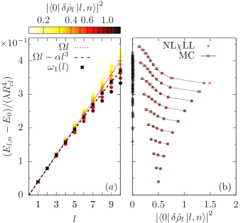
Figure 1: (a) Numerical results for the energy spectrum $E_{l,n}-E_{0}$ of a FQH cloud confined by a quartic $V_{\rm conf}(r)=\lambda r^{4}$ trap. Eigenstates are plotted against their angular momentum $l$ and are coloured according to their DSF weight $|\bra{0}\delta\hat{\rho}_{l}\ket{l,n}|^{2}$. The red dotted line is the linear dispersion of the edge modes, $\Omega l$; the black line includes the cubic correction, $\Omega l-\alpha l^{3}$. Black circles with crosses indicate the center-of-mass (18) of the DSF. (b) Plot of the DSF (on the $x$-axis) against the excitation energies $E_{l,n}-E_{0}$ (on the $y$-axis). The black circles are the result of full 2D numerical calculations, while the red crosses are the predictions of the NL-$\chi$LL  model of Eq. (4). For each angular momentum $l$, the main emerging structures have been joined with black-dashed lines as a guide for the eye. Both panels are for $N=25$ bosons at $\nu=1/2$ filling.

As long as we neglect the coupling to states above the many-body energy gap and we restrict to excitation frequencies $\omega$ below the many-body energy gap, the DSF (15) can be rewritten by introducing a projector onto the relevant low-energy subspace, which gives

$$S_{l}(\omega)=\sum_{n}\,\delta\left(\omega-\omega_{l,n}\right)\left|\bra{0}\delta\hat{\rho}_{l}\ket{l,n}\right|^{2}\,.$$ (17)

Here, $n$ runs through the excited states of angular momentum $l$ and $\omega_{l,n}=E_{l,n}-E_{0}$ is their energy difference from the Laughlin ground state. In our previous work Nardin and Carusotto (2023), we computed this quantity both via a full 2D numerical calculation of the FQH cloud and via the NL-$\chi$LL  model of Eq. (4). As it is displayed in Fig. 1, the results of the two methods are in excellent quantitative agreement.

We here wish to highlight the importance of the dispersion and interaction terms in Eq. (4). Even though for a fixed $l$ most of the DSF weight is concentrated in the lowest energy states, a non-zero weight is present in higher energy states as well. As a result, the dispersion of linear waves, defined as the center-of-mass of the DSF

$$\omega_{1}(l)=\frac{\int\omega S_{l}(\omega)d\omega}{\int S_{l}(\omega)d\omega},$$ (18)

does not coincide with the lowest energy state at $E_{-}(l)$. It is henceforth not possible to identify this state with a single boson excitation at the same angular momentum $l$, as previously done Stone et al. (1992); Wan et al. (2003, 2008); Jolad and Jain (2009); Jolad et al. (2010). The boson-boson interaction term proportional to $\hat{\rho}^{3}$ in the NL-$\chi$LL  model of Eq. (4) is therefore playing a crucial role in spreading the DSF over a finite range of energies. Furthermore, as we are going to see in the next Sections, the fact that $\omega_{1}(l)$ deviates from a linear behaviour highlights the importance of the dispersive term proportional to $(\partial_{\theta}\hat{\rho})^{2}$.

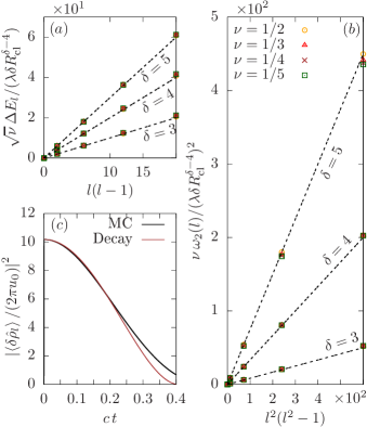
Figure 2: (a) Plot of the (normalized) total width $E_{+}(l)-E_{-}(l)$ defined in Eq. (21) as a function of the (rescaled) angular momentum $l(l-1)$. The results of full 2D numerical calculations for various values of $\nu$ and $\delta$ accurately follow the behaviour $\sqrt{\nu}\Delta E_{l}/(\lambda\delta R_{cl}^{\delta-4})=(\delta-2)l(l-1)$ predicted by Eq. (21) together with Eq. (7), shown here as black-dashed lines. (b) Plot of the second moment $\omega_{2}(l)$ of the DSF as a function of the (rescaled) angular momentum $l^{2}(l^{2}-1)$. The results of the full 2D numerical calculations for various values of $\nu$ and $\delta$ accurately follow the behaviour $\nu\omega_{2}(l)/(\lambda\delta R_{cl}^{\delta-4})^{2}=(\delta-2)^{2}l^{2}(l^{2}-1)/12$ predicted by Eq. (24) together with Eq. (7), shown here as black-dashed lines. (c) Time-evolution of the square modulus of the fundamental component of the edge-density response in response of a weak pulsed excitation of strength $u_{0}$ and angular momentum $l=3$. The black curve is the result of the full 2D numerical calculation, while the brown curve is the the short-time decay prediction of Eq. (28). In all panels, a FQH cloud of $N=25$ particles is considered.

IV.1.1 Broadening of the dynamic structure factor

As a first application of the refermionized Hamiltonian Eq. (11), we look at the broadening of the DSF that is well visible in Fig. 1 and manifests as a progressive spreading of the energies with the angular momentum $l$ of the cloud.

In order to get a simple picture of the underlying physics, we start by making the approximation of neglecting the interactions between fermions described by the last term of the Hamiltonian (11). This leaves us with a free fermion model of dispersion $\epsilon_{l}$ whose excitations consist of particle-hole pairs around the Fermi level, taken to be at $l_{F}=0$. Within this approximation, for a given value of the angular momentum $l$ of the excitation, the DSF has a flat profile in between the least and the most energetic excitations, whose energies are respectively equal to

$$E_{+}(l) = \epsilon_{l}-\epsilon_{0}$$ (19)

$$E_{-}(l) = \epsilon_{1}-\epsilon_{1-l}\,.$$ (20)

Taking the difference of these energies gives an estimate for the total broadening

$$\Delta E_{l}=E_{+}(l)-E_{-}(l)=\frac{c}{\sqrt{\nu}}\,l(l-1),$$ (21)

which is proportional to the trap curvature parameter $c$ and grows quadratically with the excitation angular momentum $l$. Interestingly, the prefactor depends on the filling fraction of the underlying FQH state. Notice that the normalized first moment of the DSF $\omega_{1}(l)$ Eq. (18) coincides in this simple case with the average

$$\omega_{1}(l)=\frac{E_{+}+E_{-}}{2}=\Omega l$$ (22)

which highlights, as we foretold above, the importance of the fermion interaction term, or, equivalently, of the additional bosonic dispersive term.

An alternative measure of the DSF broadening is provided by the second moment of the DSF

$$\omega_{2}(l)=\frac{\int(\omega-\omega_{1}(l))^{2}S_{l}(\omega)\,d\omega}{\int S_{l}(\omega)d\omega}\,,$$ (23)

which, for the flat DSF of non-interacting fermions, is equal to

$$\omega_{2}(l)=\frac{c^{2}}{\nu}\,\frac{l^{2}(l^{2}-1)}{12}.$$ (24)

The two broadening measures Eq. (21) and Eq. (24) are compared with microscopic Monte Carlo data for different values of the exponent $\delta$ of the confinement potential and of the filling factor $\nu$ in Fig. 2(a) and Fig. 2(b) respectively. For both quantities, the analytical predictions appear to accurately capture the numerical data, especially for low values of the filling fraction $\nu$ and of the confinement exponent $\delta$: this regime allows in fact to minimize effects caused by the gradient of the curvature parameter $c$, which is neglected in our NL-$\chi$LL  theory. As a further evidence in support of our conclusions, more numerical results on the quartic $\delta=4$ case are shown in Appendix A.

From an experimental perspective, besides the spectroscopic measurements of Fabbri et al. (2015) the second moment Eq. (24) of the DSF can be indirectly measured by looking at the short- and moderate-time part of the temporal decay of edge-density excitations on top of the FQH cloud. Consider that the cloud is excited via a time-dependent perturbation $U(\theta,t)$ whose strength is almost constant in the vicinity of the classical radius. Using linear perturbation theory, we obtain the following result for the edge-density response

$$\braket{\delta\hat{\rho}(\theta,t)}=\frac{1}{\pi}\Im\left[\sum_{l}e^{il\theta}\int\widetilde{U}_{l}(\omega)\,S_{l}(\omega)\,e^{-i\omega t}\,d\omega\right]$$ (25)

where $\widetilde{U}_{l}(\omega)$ is the Fourier transform of the excitation potential and $S_{l}(\omega)$ the DSF defined in Eq. (15).

Assuming that the spectrum $\widetilde{U}_{l}(\omega)$ of the perturbation is approximately constant across the peak of $S_{l}(\omega)$ (this requires that the excitation pulse is sufficiently short compared to the characteristic time-scale of the edge dynamics), we can approximate the integral appearing on the right-hand side of (25) as

$$\widetilde{U}_{l}(\omega_{1}(l))e^{-i\omega_{1}(l)t}\int\,S_{l}(\omega)\,e^{-i(\omega-\omega_{1}(l))t}\,d\omega.$$ (26)

Up to not-too-large times, the exponential inside this integral can be expanded to second order, which gives

$$\widetilde{U}_{l}(\omega_{1}(l))e^{-i\omega_{1}(l)t}\times\\ \times\int\,S_{l}(\omega)\,\left(1-\frac{(\omega-\omega_{1}(l))^{2}t^{2}}{2}\right)\,d\omega\,.$$ (27)

Then, using the sum-rule $\int S_{l}(\omega)\,d\omega=\nu l\,\Theta(l)$ for the static structure factor of a FQH cloud in the thermodynamic limit ($\Theta$ is here the Heaviside step function), we finally get

$$\braket{\delta\hat{\rho}(\theta,t)}\simeq-\frac{\nu}{\pi}\sum_{l>0}\left(1-\frac{\omega_{2}(l)t^{2}}{2}\right)\times\\ \times\frac{\partial}{\partial\theta}\,\Re\left[e^{i(l\theta-\omega_{1}(l)t)}\widetilde{U}_{l}(\omega_{1}(l))\right]\,:$$ (28)

at short times after the excitation, the decay of density modes follows a quadratic law. Its time-scale is set by the second moment of the DSF which, in turn, depends on the curvature parameter $c$ and on the filling fraction of the bulk, $\nu$ according to Eq.(23). As a sidenote, notice that it is indeed $\omega_{1}(l)$ [Eq. (18)] which sets the propagation velocity.

The accuracy of the approximated expression Eq. (28) at short times is successfully validated against the exact evolution in Fig. 2(c), where we plot the response of the edge modes to an excitation carrying definite angular momentum. These results support a physical interpretation of the edge excitation decay as the result of the decoherence of the different particle-hole excitations that we originally proposed in Nardin and Carusotto (2020) for the IQH case.

To conclude this Subsection, it is interesting to highlight that the formulas Eq. (21) and Eq. (24) for the DSF broadening, obtained neglecting interactions between fermions, remain accurate well outside the regime where interactions are irrelevant. The non-interacting fermion approximation predicts in fact the DSF to be flat and centered at the linear $\chi$LL dispersion [Eq. (22)] $\omega_{1}(l)=\Omega l$; however, as one can see in Fig. 1, while $\omega_{1}(l)$ only slightly deviates from the linear behaviour over the values of $l$ considered in Fig. 2, the DSF rapidly starts acquiring a highly non-trivial lineshape much before the non-interacting fermion approximation for the broadening breaks down. Analogously, while the broadening $\Delta E_{l}$ in Eq.(21) compares remarkably well with the full 2D numerical calculation, the threshold energies $E_{\pm}$ predicted by the non interacting model Eq. (19) separately do not.

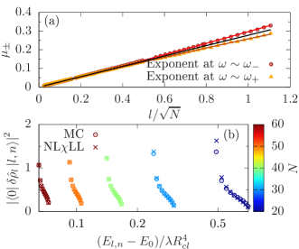
Figure 3: (a) Plot of the DSF threshold exponents $\mu_{\pm}$ as a function of the excitation momentum $q=l/R_{cl}\propto l/\sqrt{N}$, numerically extracted from the predictions of the NL-$\chi$LL model of Eq. (4) by means of a power-law fit to the DSF data close to the lower and upper threshold. The extracted exponents at the lower and upper thresholds are shown as red circles and yellow triangles, respectively, and are quite successfully compared to the mobile-impurity result of Eq. (30) shown as a black line. An even better agreement is found including a phenomenological quadratic correction as done in Eq. (31) (red and brown lines). (b) Comparison between the microscopic DSF weigths extracted from full 2D numerical calculations (circles) and those obtained from the NL-$\chi$LL model Eq. (4) (crosses) for different particle numbers $N$ (colorscale) at a fixed angular momentum $l=10$. The DSF weights are plotted against the excitation energies in a logarithmic scale.

IV.1.2 Threshold singularities of the dynamic structure factor

On top of the broadening effect discussed in the previous Subsection, the curves for the DSF plotted in Fig. 1(b) for growing $l$ clearly show the appearance of some peculiar singular behaviours close to the spectral thresholds. Such features are reminiscent of those emerging from the theory of non-linear (non-chiral) Luttinger liquids Imambekov et al. (2012).

The main challenge in the theoretical study of both the bosonic and fermionic models of Eq. (4) and Eq. (11) comes from the fact that both the group velocity dispersion and the non-linearity are proportional to the same curvature parameter $c$. For this reason, perturbative approaches based on a hydrodynamic formulation where dispersion dominates over interactions Price and Lamacraft (2014, 2015) do not give consistent results. On the other hand, many features of the fermionic theory Eq. (11), in particular the behaviour around the energy thresholds, can be be successfully studied making use of so-called “mobile-impurity” approaches.

Within a non-interacting fermion model, the lower threshold corresponds to the displacement of a particle from deep below the Fermi point to right above it and, correspondingly, the upper threshold corresponds to the displacement of a particle initially located at the Fermi point up to high energy states. These processes can be seen as the creation of a deep-hole or a high-energy-particle accompanied by a slight shift of the Fermi point (sketched in the last or first row of Fig. 4, respectively). Once we include again interactions, if we focus on the threshold regions, the interacting fermion theory of Eq. (11) can be replaced by an effective two-band model, namely a (chiral) Luttinger liquid at $l\sim 0$ and a single deep-hole/high-energy-particle at $l$ Pustilnik et al. (2006); Khodas et al. (2007); Imambekov et al. (2012). This latter then acts as an impurity off which particles close to the Fermi point, that is the Luttinger liquid, can perform small-momentum-transfer scattering processes. As it is discussed in detail in Pustilnik et al. (2006), such processes lead to a power-law enhancement of the DSF close to the lower-energy threshold $\omega_{-}(l)$ and a corresponding power-law suppression at the high-energy threshold $\omega_{+}(l)$. In formulas, we have that

$$\begin{cases}S_{l}(\omega\sim\omega_{-})\propto\theta(\omega-\omega_{-})\left(\frac{1}{\omega-\omega_{-}}\right)^{\mu_{-}}\\ S_{l}(\omega\sim\omega_{+})\propto\theta(\omega_{+}-\omega)\left(\omega_{+}-\omega\right)^{\mu_{+}}\end{cases}$$ (29)

where the exponents

$$\mu_{+}\simeq\mu_{-}\simeq\frac{2\alpha l}{c/\sqrt{\nu}}=2\beta_{\nu}\sqrt{\nu}\,\frac{l}{R_{cl}}$$ (30)

only depend on the excitation momentum $l/R_{cl}$ and the bulk filling fraction $\nu$, but not on the specific values of the non-universal trap parameters $\Omega$ and $c$. Even though a finite value of $c$ is essential for the emergence of the singular power-law behaviour, the value of the exponents turn out to be universal properties of strongly correlated FQH fluids with short-ranged interactions, a manifestation of strong bulk correlations extending all the way through the edge. This peculiar universal behaviour emerges because the exponent is set by $2m^{*}\alpha$, but both the effective mass $m^{*}$ and the interaction strength proportional to $\alpha$ emerge because of the presence of the trap causing a gradient of angular velocity at the cloud’s edge. So, while $\alpha$ is directly proportional to $c$, the effective mass $m^{*}$ is inversely proportional to it: the curvature parameter $c$ therefore cancels out from the exponents $\mu_{\pm}$.

A direct validation of the power-law behaviour via full two-dimensional simulations of the FQH clould is made difficult by the fast, almost exponential ($\log\mathcal{D}\propto\sqrt{l}$) growth of the Hilbert space dimension $\mathcal{D}$ at the large angular momentum $l$ values that are needed to interpolate power-law behaviours at both thresholds.

In our previous work Nardin and Carusotto (2023) and in the previous Sections, we have seen a quantitative agreement between full two-dimensional numerical simulations and the predictions of the NL-$\chi$LL theory of Eq. (4). This statement is further validated in Fig. 3(b) where we compare the DSF weights for increasing number of particles $N$ at fixed angular momentum $l$: as the excitation wavevector $q=l/R_{cl}\propto l/\sqrt{N}$ decreases the NL-$\chi$LL model becomes even more accurate, so we can expect it to correctly account for the behaviour of the DSF in the thermodynamic limit. On this basis, we restrict our numerical analysis to the NL-$\chi$LL theory which grants us access to the large $l$ values that are needed to precisely extract the power law exponents.

The numerical predictions for the exponents at the lower and higher thresholds are plotted in Fig. 3(a): a good agreement with the analytical prediction of Eq. (30) is found for small values of the wavevector $q$, with quadratic corrections at higher $q$ phenomenologically compatible with the form

$$\mu_{\mp}=\pm\left[\left(1\pm\frac{\alpha l}{c/\sqrt{\nu}}\right)^{2}-1\right].$$ (31)

These results illustrate the power of the refermionized theory in capturing the peculiar behaviour of the neutral edge excitations of a FQH cloud and show that the FQH edges indeed behave as a peculiar example of nonlinear Luttinger liquid Imambekov et al. (2012).

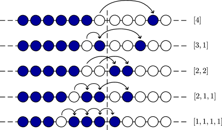
Figure 4: Schematic diagram of the different particle-hole excitations (black-arrows) across the Fermi point (vertical-dashed lines) at a fixed angular momentum $l=4$. For each state, the corresponding partition of $l=4$ are indicated on the right-hand side of the plot.

IV.1.3 Fine structure of the dynamic structure factor

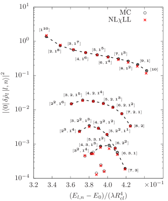
Figure 5: Plot of the DSF weights $|\bra{0}\delta\hat{\rho}_{l}\ket{l,n}|^{2}$ against the excitation energy $E_{l,n}-E_{0}$ for a $l=10$ excitation of a FQH cloud of $N=25$ bosons at filling $\nu=1/2$ confined by a quartic $\delta=4$ trap. The black circles are the result of a full 2D numerical calculation and are compared to the predictions of the NL-$\chi$LL  model of Eq. (4). Differently from Fig. 1(b), the weights are plotted here in logarithmic scale. All points with a sizable DSF weight are labeled in terms of the partition $\eta$ corresponding to the particle-hole excitation which has a strongest overlap with the eigenstate.

Going beyond the mesoscopic quantities investigated in the previous Subsections, it is interesting to see how the refermionized theory provides an interesting physical interpretation also for the microscopic structure of the eigenstates, in particular the values of the matrix elements $|\bra{0}\delta\hat{\rho}_{l}\ket{l,n}|^{2}$ entering the DSF. As an example, a plot of these matrix elements is displayed in Fig. 5 for the $l=10$ case.

Within the fermionic model, we expect that at the level of the free fermion approximation, the $\delta\hat{\rho}_{l}$ operator only connects the ground state Fermi sea to the single particle-hole states on top of it (first, second, fourth and fifth rows of Fig. 4) and that the $l$ such transitions have the same amplitude. This simple picture is of course modified by the presence of fermionic interactions, so that non-zero matrix elements may appear also for states corresponding to several particle-hole excitations (third line of Fig. 4).

This expectation is fully confirmed by the numerical data shown in Fig. 5. As it is displayed in Fig.10 of Appendix C, the interacting eigenstates are found to maintain a dominant weight on the particle-hole basis of non-interacting fermions. On this basis, in Fig. 5 we keep labelling the states in terms of the partition $\eta$ of the non-interacting particle-hole state which has the largest weight on the eigenstate. As usual, a partition $\eta=[\eta_{1},\eta_{2},\eta_{3}\ldots]$ is defined to have $\eta_{1}\geq\eta_{2}\geq\eta_{3}\geq\ldots$ and corresponds to a state where, starting from a filled Fermi sea, the highest energy particle is promoted by $\eta_{1}$ orbitals, the second-highest one by $\eta_{2}$ orbitals and so on: for the sake of clarity, a few examples of partitions and of the corresponding states are illustrated in Fig. 4.

From Fig. 5, it is apparent how the matrix elements tend to organize in a hierarchical way. Besides the principal sequence of highest-weight states corresponding to single particle-hole excitations discussed above, well-distinguishable secondary sequences of states are visible, carrying a much weaker DSF weight. For all these data-points, an excellent agreement is found between the NL-$\chi$LL model and the full two-dimensional calculation.

While this latter method gets quickly impracticable for larger values of $l$, the NL-$\chi$LL model provides a manageable and reliable approach up to much larger $l$ values. An example of such calculation is displayed in Fig.6: thanks to the larger $l=20$ value, a larger number of secondary structures is clearly discernible. Interestingly, these structures can be grouped together (black-dashed lines) by considering squeezing processes in which the high-energy fermion looses one unit of angular momentum by exciting one more fermion across the Fermi point that delimits the Fermi sea of filled states, e.g. $[7,3]\rightarrow[6,3,1]\rightarrow[5,3,1,1]\rightarrow\ldots[3,3,1,1,1,1]$.

As a final point, it is interesting to look at these structure from the point of view of the two-dimensional FQH cloud. Remarkably, we find a large overlap ($\gtrsim 95\%$ for the considered system sizes) between the eigenstates of the 2D FQH system and Jack polynomial states Macaluso and Carusotto (2017, 2018) labeled by the same partitions $\eta$. The interested reader can find a color plot of the overlap matrix in Fig.9 of Appendix C, together with a brief description of the numerical method used to compute them. While no complete explanation of this remarkable result is available yet, it hints at a deep relation between the Pauli principle for the fermions of the refermionized theory and the generalized Pauli principle naturally implemented by the Jacks Bernevig and Haldane (2008). A complete understanding of this relation will be the subject of future work.

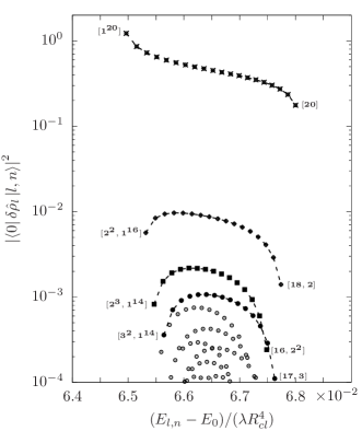
Figure 6: Plot of the DSF weights $|\bra{0}\delta\hat{\rho}_{l}\ket{l,n}|^{2}$ against the excitation energy $E_{l,n}-E_{0}$ for a $l=20$ excitation of a FQH cloud of $N=300$ bosons at filling $\nu=1/2$ confined by a quartic $\delta=4$ trap. The points have been computed via the NL-$\chi$LL  model of Eq. (4).

IV.2 Spectral function

Another quantity of great interest in the study of Luttinger liquids is the SF, which describes the probability of removing a particle from the system at a given energy. This quantity is relevant for the study of particle tunneling into $\chi$LL and is connected to power-laws in the current-voltage characteristic of FQH systems Wen (1991b). Recently it was shown to contain relevant information on Haldane fractional exclusion statistics Cooper and Simon (2015) and to be directly accessible to experiments in various synthetic setups Cooper and Simon (2015); Umucal ılar and Carusotto (2017).

Focusing on the $\nu=1/2$ bosonic Laughlin state at $\nu=1/2$, in this Subsection we show how the results of the full two-dimensional calculation of the SF are quantitatively captured by NL-$\chi$LL model of Eq. (4) once this is supplemented with the bosonized form of the particle annihilation operator Wen (1992)

$$\hat{\psi}(\theta)=e^{-i\hat{\phi}(\theta)/\nu}$$ (32)

in terms of a bosonic phase operator $\hat{\phi}$ related to the density through $\hat{\rho}=-\partial_{\theta}\hat{\phi}/2\pi$ Wen (1992, 1995). The refermionized approach is then used to shine physical light on the peculiar properties of the SF.

IV.2.1 Comparison with full 2D numerical calculations

As usual, we define the SF as

$$A_{l}(\omega)=\sum_{f}\left|\bra{f}\hat{a}_{(N-1)/\nu-l}\ket{0}\right|^{2}\delta(\omega-\omega_{f,0}).$$ (33)

where the sum runs over all $N-1$ particle states $\ket{f}$ and $\ket{L_{N}}$ is the $N$ particle Laughlin ground state. Here, $\hat{a}_{(N-1)/\nu-l}$ annihilates a particle with angular momentum $(N-1)/\nu-l=\Delta l$. The reason behind this notation for the angular momentum will be clarified shortly.

Let us first notice that, provided the anharmonic confinement does not induce mixing of the low-lying edge excitations with states above the many-body gap, the frequency-integrated SF $A_{l}=\int d\omega\,A_{l}(\omega)$ at fixed $l$ is independent of the specific confinement as the eigenstates $\ket{f}$ are connected by a unitary transformation. The standard $\chi$LL result $A_{l}\propto l^{1/\nu-1}$ (at small values of $l$) is therefore maintained in spite of the SF being broadened and having a highly non-trivial line-shape. As such, we focus here on the energy-resolved $A_{l}(\omega)$.

The initial $N$ particle Laughlin state has total angular momentum $L_{0}^{(N)}=N(N-1)/(2\nu)$. The occupied single-particle orbital of largest angular momentum has angular momentum $(N-1)/\nu$, so the angular momentum $L_{f}$ of the final state after removing one particle lies in the range

$$\frac{(N-1)(N-2)}{2\nu}\leq L_{f}\leq\frac{N(N-1)}{2\nu}\,,$$ (34)

that is, between $L_{0}^{(N-1)}$ and $L_{0}^{(N)}$. For convenience, we will focus our attention on the removal of a particle close to the edge of the system. Since such a particle carries a large angular momentum $\lesssim(N-1)/\nu$, the final state can be seen as a low-angular-momentum edge-excitation with angular momentum $l$ with respect to the $N-1$ particles-Laughlin ground state; therefore, the relevant matrix elements can be studied through the NL-$\chi$LL  model of (4).

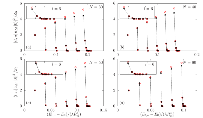
Figure 7: SF weight $|\bra{f}\hat{a}_{(N-1)/\nu-l}\ket{0}|^{2}$, normalized to the $l=0$ Laughlin-Laughlin matrix element $Z_{0}=|\bra{f}\hat{a}_{(N-1)/\nu}\ket{0}|^{2}$. Black points are the result of the full 2D numerical calculation for bosons at a constant filling $\nu=1/2$ in a quartic $\delta=4$ trap but different numbers of particles in each panel: (a) $N=30$, (b) $N=40$, (c) $N=50$ and (d) $N=60$. The red circles display the predictions of the NL-$\chi$LL model of Eq. (4). The insets display a magnified view of the $l=6$ curves. Amplitudes relative to different $l$-sectors ($l=1\ldots 6$) have been joined with black dashed lines as a guide for the eye. The point corresponding to $l=0$ is not shown as it equals $1$ by definition due to the normalization factor.

Within our theoretical framework, we calculate the matrix elements appearing in Eq. 33 through a Monte-Carlo sampling of the full two-dimensional wavefunctions, as described in Appendix D. The results of this microscopic calculation are shown in Fig. 7 and are compared to the prediction of the NL-$\chi$LL model. In this latter calculation, the single-particle destruction operators $\hat{a}_{\Delta l}$ of the full two-dimensional theory are interpreted within the $\chi$LL framework as

$$\hat{a}_{\Delta l}=\int d\theta\,\frac{e^{i\,\Delta l\,\theta}}{\sqrt{2\pi}}\,\hat{\psi}(\theta)\,,$$ (35)

where the bosonized form Eq.(32) of the annihilation operator is used. In order to remove an overall normalization factor which ambiguously depends on the cutoff length-scale of the effective edge-boson theory Palacios and MacDonald (1996); Jolad et al. (2007); Jolad and Jain (2009); Jolad et al. (2010); Giamarchi and Press (2004), all matrix elements have been normalized to the Laughlin-Laughlin transition matrix element $Z_{0}=|\bra{L_{N-1}}a_{(N-1)/\nu}\ket{L_{N}}|^{2}$. As expected, only a limited number of states within each angular momentum $L_{f}=L_{0}^{(N-1)}+l$ sector have a significant matrix element.

A good qualitative and quantitative agreement between the two theories is clearly visible in Fig. 7, in particular for the low-energy states at low $l$. At large $l$, a good agreement is recovered as the system is made larger and the wavelenght gets correspondingly longer. Most interestingly, these numerical results prove the correctness of the exponential expression Eq.(32) for the particle annihilation operator in terms of the bosonic field within our NL-$\chi$LL model Eq. (4).

IV.2.2 Behaviour of the SF at the energy thresholds

Following Cooper and Simon (2015) and based on the microscopic insight discussed in the previous Sec.IV.1.3, we can identify the states corresponding to the energetic thresholds of $A_{l}(\omega)$: the lower threshold corresponds to the state labelled by the partition $[1^{l}]$, while the upper threshold corresponds to the state of partition $[2^{l/2}]$ if $l$ is even or $[2^{(l-1)/2},1]$ if $l$ is odd. These partitions have a simple interpretation in terms of the fermionic model: as in the DSF case, the state at the lower threshold of the SF has a deep-hole at $\sim-l$ (an impurity) off which particles at the Fermi point at $l=0$ (i.e. the Luttinger liquid) can scatter with small angular momentum exchanges. On the other hand, the state at the upper threshold displays a pair of deep holes at $\sim-l/2$ and dramatically differs from the (higher energy) state with a high-energy particle at $\sim l$ related to the upper threshold of the DSF. Therefore, the upper threshold of the SF does not correspond to the highest energy eigenstate at the given angular momentum $l$.

For small systems, our results are in agreement with exact diagonalization results and with the counting prescription derived from Haldane’s fractional exclusion statistics principle Haldane (1991); Bernevig and Haldane (2008) as discussed in Cooper and Simon (2015). Thanks to the larger values of $N$ accessible to our calculations, we find that this counting prescription remains accurate for odd values of $l$ for growing $N$, while for even $l$ one state ends up eventually losing all its SF weight. A precursor of this difference can already be appreciated for the moderate system sizes considered in Cooper and Simon (2015): a single state has a systematically smaller spectral weight for even $l$ than for odd $l$ values. This different behaviour can be attributed to the qualitatively different structure of the state with the smallest possible SF weight at a given $l$, that is the state closest to the upper threshold, which corresponds to the $[2^{l/2}]$ and $[2^{(l-1)/2},1]$ partitions for respectively even and odd values of $l$. This unexpected suppression of the spectral weight is even more remarkable if one thinks the state of partition $[2^{l/2}]$ as the result of removing one particle of well-defined angular momentum $(N-1)/\nu-l$ from the $N$ particle Laughlin state partition, which is equivalent to the creation of a double quasihole at the same angular momentum. All other states with non-zero spectral weight correspond instead to the insertion of two quasiholes with distinct values of the angular momentum.

In analogy to the DSF shown in Fig. 1, also the SF displays a marked singularity at the lower threshold within each $l$ sector. The characterization of the functional form of the threshold behaviour however appears to be far more challenging than in the DSF case, and no robust conclusion can yet be drawn from the available theoretical insight and numerical data.

From the theoretical side, a study of the SF threshold within the bosonized theory is made difficult by the exponential form Eq. (32) of the single-particle annihilation operator, to be contrasted to the expression (15) of the DSF that directly involves the density operator $\hat{\rho}$. It is reasonable to think that the refermionized model may still be relevant for extracting information on the SF, especially at the lower energy threshold which, as we discussed above, corresponds to a simple situation in which a Luttinger liquid scatters from a deep-hole. However, a naive attempt to express the bosonized form of the particle annihilation operator Eq. (32) in terms of the fermions $e^{-i\hat{\phi}(\theta)/\nu}=e^{-i\hat{\phi^{\prime}}(\theta)/\sqrt{\nu}}\sim\Psi^{1/\sqrt{\nu}}$ leads to an ill-defined operator, whose value to characterize the SF singularities using a mobile-impurity model Imambekov et al. (2012) is far from obvious and calls for more sophisticated treatment.

Serious difficulties are also present from the numerical side. Testing the power-law behaviour by fitting the SF $A_{l}(\omega)$ computed with the NL-$\chi$LL model requires working at even larger $l$ values than for the DSF case as the number of points that are available to the fit for given $l$ is roughly halved as compared to the DSF case. Moving to higher $l$ values forces to work in larger Hilbert spaces leading to an intractable numerical complexity of the calculation.

In spite of these theoretical difficulties, the SF remains a quantity of key experimental interest. On one hand, it can be directly probed in the single-particle spectroscopy experiments proposed for FQH clouds of atoms or photons in Cooper and Simon (2015); Umucal ılar and Carusotto (2017). Specially in the photonic case the SF is directly observable from the emission spectrum of the fluid, so our predictions are of direct application to the experiments. On the other hand, a complete understanding of the SF will be instrumental to attack the harder questions related to the non-perturbative dynamics of the edge: large density dips at the edge of the FQH cloud can in fact be be produced by selectively removing particles close to the edge of the cloud. It is therefore very interesting to investigate the emerging non-linear Korteweg-de Vries hydrodynamics described by Eq. (4), which, analogously to what occurs at the classical level, may lead to shockwaves and solitons that chirally propagate along the edge, a possibility already pointed out in Bettelheim et al. (2006); Wiegmann (2012).

V Conclusions

In this work we have shown how the nonlinear chiral Luttinger liquid description of the low-energy dynamics of the edge modes of a fractional quantum Hall cloud introduced in Nardin and Carusotto (2023) can be conveniently reformulated in terms of a model of massive and interacting chiral fermions in one-dimension. Exploiting the physical insight offered by applying Tomonaga-Luttinger liquid techniques to the refermionized theory, we investigate the dynamic structure factor and the spectral function of the fractional quantum Hall fluid, providing quantitative explanations to the numerical predictions of full two-dimensional simulations of the fractional quantum Hall cloud. In particular, our refermionized theory offers a physical interpretation to the dynamic structure factor broadening, which sets the edge-mode-decay time-scale. Building on established results for quantum impurity models in Luttinger liquids Imambekov et al. (2012), we then investigate momentum-dependent power-law behaviour shown by the DSF close to its spectral edge: the exponents turn out to be universal, for they only depend on the bulk filling fraction $\nu$ but are otherwise independent on the details of the confinement potential. We then show how the nonlinear chiral Luttinger liquid model provides accurate information also on the spectral function describing the energy-dependence of the particle removal process. The quantitative agreement with the full 2D numerical calculation showcase the accuracy of the exponential form of the bosonized destruction operator within the nonlinear chiral Luttinger liquid theory. Since the equation of motion of the edge-density operator has a Korteweg-de Vries form in the classical limit, and such an equation is well-known to admit solitonic solutions, a future task will be to address the emergent dynamics of the large density depletions caused by the removal of a particle close to the edge and investigate whether shock-wave-like behaviours can lead to the formation of solitons Bettelheim et al. (2006); Wiegmann (2012).

Since our conclusions are based on a very generic model with short-ranged interactions, we anticipate that they straightforwardly apply to fractional quantum Hall fluids in either atomic or photonic synthetic quantum matter. As such, they are ready to be experimentally verified with state-of-the-art technology and hold a great promise as a novel probe of the bulk topological order and its anyonic excitations. Future efforts will be devoted to the generalization of our approach to the study of long-range interacting systems, to understand the interplay between the confinement-induced physics studied here and the non-vanishing interaction energy in a two-dimensional electron gas in solid-state devices. Further steps will address exotic non-abelian quantum Hall states, such as the Moore-Read Moore and Read (1991), which do host a more complex manifold of edge modes. On a longer run, we believe our results will contribute paving the way towards the study of fractional quantum Hall fluids as a novel platform for nonlinear quantum optics of edge excitations with unprecedented dynamical and statistical properties.

Appendix A DSF broadening in a quartic trap

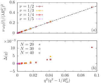
Figure 8: (a) Plot of the (normalized) second moment $\omega_{2}$ of the DSF in a quartic $\delta=4$ trap, for different system sizes $N$ and filling fractions $\nu$. In order to highlight the long-wavelength limiting behaviour, we plot $\omega_{2}$ as a function of $q^{2}(q^{2}-1/R_{cl}^{2})$ rather than $l^{2}(l^{2}-1)$ where $q$ is the physical wavevector $q=l/R_{cl}$ of the edge excitation. The result of the full 2D numerical calculation (symbols) is compared with the analytical prediction Eq. (24) of the non-interacting fermion approximation (black-dashed line). (b) Difference between the numerical and the analytical results shown in (a): the difference tends to zero in the $q\to 0$ long wavelength limit.

In this first Appendix A, we present a more detailed analysis of the second moment

$$\omega_{2}(l)=\frac{\int(\omega-\omega_{1}(l))^{2}S_{l}(\omega)d\omega}{\int S_{l}(\omega)d\omega}$$ (36)

of the edge DSF in the case of a weak quartic $V_{\text{conf}}=\lambda r^{4}$ potential confining the FQH cloud and we compare the result to the theoretical prediction of Eq. (24). This case is particularly simple: in the quartic trap, the angular velocity gradient (the second derivative with respect to the angular momentum $\partial_{l}=\frac{\partial r}{\partial l}\,\partial_{r}\approx r^{-1}\partial_{r}$) at the position of the cloud’s edge is in fact constant and position independent [Eq. (7)],

$$c=\left.(r^{-1}\partial_{r})^{2}\,V_{\text{conf}}\right|_{r=R_{cl}}=8\lambda$$ (37)

so we have [Eq. (24)]

$$\omega_{2}(l)=\frac{16\lambda^{2}}{3\nu}\,l^{2}(l^{2}-1)\,.$$ (38)

When the product $\nu\times\omega_{2}(l)$ is plotted, data from different filling factors $\nu$ are expected to collapse on the same curve. In order to better highlight the long-wavelength limit, data for different values of the particle number $N$ and filling factor $\nu$ are plotted in terms of $q^{2}(q^{2}-R_{cl}^{-2})$, where $q=l/R_{cl}$ is the physical wavevector of the edge excitation: it is apparent how all points accurately fall on the expected straight line Eq. (38). The difference $\Delta(q)$ from this line are shown in the bottom panel: the difference is always small and tends to zero in the long-wavelength limit.

Appendix B Full 2D simulations: the numerical method

In this second Appendix B we briefly describe the numerical method used in the full two-dimensional calculations. While the general idea of the method was first introduced in Nardin and Carusotto (2023), here we made a few additions to it.

In the absence of any confinement potential, the Laughlin state Eq. (1) and its edge-excitations Eq. (3) are degenerate zero-energy eigenstates of specific model Hamiltonians with short-range interactions Haldane (1983); Trugman and Kivelson (1985); Simon et al. (2007a, b).When we include a cylindrically-symmetric confinement $V_{\text{conf}}(r)$ potential, the eigenstates of the system can be still labeled by an angular momentum quantum number $L=L_{0}+l$, where $L_{0}$ is the angular momentum of the Laughlin ground state and $l\geq 0$ the additional angular momentum carried by the chiral edge excitation. We furthermore consider the confinement to be weak compared to the interaction energy, $V_{\text{conf}}(R_{cl})\ll V_{\text{int}}$, and radially smooth, so that mixing with states above the many-body energy gap can be neglected.

Under this simplifying assumption each many-body eigenstate $\ket{l,n}$ can be expanded over the Laughlin states basis as

$$\ket{l,n}=\sum\sum_{\alpha_{l}}C_{\alpha_{l}}^{[l,n]}\frac{\ket{\alpha_{l},l}}{\sqrt{\braket{\alpha_{l},l}{\alpha_{l},l}}}$$ (39)

where the states $\ket{\alpha_{l},l}$ are a basis of linearly independent but not necessarily orthogonal states spanning the space of edge excitations at angular momentum $L_{0}+l$.

In particular, the index $\alpha_{l}$ runs through the $p_{N}(l)$ states corresponding to the integer partitions of $l$ of length smaller or equal to $N$. In practice, the $P_{\alpha}$ polynomials of Eq. (3) at a given angular momentum Halperin and Jain (2020) are expanded in a basis formed by all the degree-$l$ polynomials that are generated as a product of several power-sum symmetric polynomials. We remark that with such a choice the states $\ket{\alpha_{l},l}$ are orthogonal only in the thermodynamic limit.

Projecting the many-body time-independent Schrödinger equation $H\ket{l,n}=E_{l,n}\ket{l,n}$ over these basis states, we obtain a Schrödinger equation in the form of a generalized eigenvalue problem for the expansion coefficients $C_{\alpha_{l}}^{[l,n]}$ appearing in Eq. (39),

$$\mathds{H}_{\beta_{l},\alpha_{l}}C_{\alpha_{l}}^{[l,n]}=E_{l,n}\,\mathds{M}_{\beta_{l},\alpha_{l}}C_{\alpha_{l}}^{[l,n]}\,.$$ (40)

Here, the matrix elements $\mathds{H}$ and $\mathds{M}$ are defined as

$$\begin{cases}\mathds{H}_{\beta_{l},\alpha_{l}}=\frac{\bra{\beta_{l},l}H\ket{\alpha_{l},l}}{\sqrt{\braket{\beta_{l}}{\beta_{l}}\braket{\alpha_{l}}{\alpha_{l}}}}\\ \mathds{M}_{\beta_{l},\alpha_{l}}=\frac{\braket{\beta_{l},l}{\alpha_{l},l}}{\sqrt{\braket{\beta_{l}}{\beta_{l}}\braket{\alpha_{l}}{\alpha_{l}}}}.\end{cases}$$ (41)

Since the kinetic energy is constant within the lowest Landau level and the two-body interaction energy is assumed to be negligible within the subspace of Laughlin-like states (it is exactly zero for the case of contact-interacting bosons at $\nu=1/2$, or for specific short-ranged interactions at more general $\nu$), the effective Hamiltonian $\mathds{H}$ only includes the confinement potential $V_{\rm conf}(r)$, while the non-orthonormality of the basis wavefunctions is accounted for by the “metric” $\mathds{M}$.

The high-dimensional integrals in Eq. (41) are computed by means of a standard Metropolis-Monte Carlo sampling  Metropolis and Ulam (1949); Metropolis et al. (1953); Hastings (1970). Since the states $\ket{\alpha_{l},l}$ and $\ket{\beta_{l},l}$ are polynomials of not-too-large degree with a Laughlin wavefunction Eq. (1) as common factor, they share most of their zeros, so the sampling procedure is highly efficient.

All other matrix elements, e.g. those appearing in the DSF and in the SF are computed in an analogous way. This calculation is performed by first using the basis $\ket{\alpha_{l},l}$ of power-sum polynomials, and then rotating the results onto the basis of system eigenstates via the eigenvector matrix Eq. (39). This eigenvector matrix thus requires to be computed with high accuracy, which typically requires a much larger number of Monte Carlo realizations than just obtaining the eigenvalues.

Appendix C Overlaps with Jack polynomials

Figure 9: Overlap matrix between the numerically obtained eigenstates $\ket{l,n}$ for a FQH cloud at $\nu=1/2$ in a quartic trap $V_{\text{conf}}=\lambda r^{4}$ and the (normalized) Jack polynomials $J_{\Omega+\eta}^{\alpha}$ with $\alpha=-2/(r-1)$ and $r=1/\nu$. On the $x$ axis, the system’s eigenvectors $\ket{l,n}$ are ordered by increasing eigenvalue number $n$. On the $y$ axis we report the Jack edge-partitions $\eta$ with which the overlap has been computed. The edge-partitions $\eta$, on the $y$-axis, have been ordered in such a way that the the largest overlap (close to $1$) lies on the diagonal.

In this third Appendix C, we explicitly show how the eigenmodes at filling $\nu=1/2$ in the quartic trap have large overlaps with a single Jack polynomial Lee et al. (2014); Macaluso and Carusotto (2017, 2018) of parameter $\alpha=-2/(r-1)$ with $r=1/\nu=2$ and labelled by a $(1,r)$-admissible root-configuration $\Omega^{\prime}$.

We expand $\Omega^{\prime}=\Omega+\eta$, where $\Omega$ is the Laughlin state root partition Bernevig and Haldane (2008) and $\eta$ is the edge-partition, labelling a basis of edge excitations at angular momentum $l$. As described in Lee et al. (2014), analogously to Eq. (3), we then have $J_{\Omega+\eta}^{\alpha}=J_{\eta}^{\beta}J_{\Omega}^{\alpha}$ where $\beta=2/(r+1)$ and $J_{\Omega}^{\alpha}$ is the Laughlin state at filling $1/r=1/2$ in our case.

Since the Laughlin state factors out, the overlaps between the eigenstates $\ket{l,n}$ and the edge-Jacks $J_{\Omega^{\prime}}^{\alpha}$ are easily computed by means of a generalization of the Monte Carlo sampling discussed above. We start by expanding the eigenstates at angular momentum $l$ as in Eq. (39) $\ket{l,n}=\sum_{\alpha_{l}}C_{\alpha_{l}}^{[l,n]}\frac{\ket{\alpha_{l},l}}{\sqrt{\braket{\alpha_{l},l}{\alpha_{l},l}}}$, so that we can express the properly-normalized matrix elements of interest as

$$\frac{\braket{l,n}{J_{\Omega^{\prime}}^{-2}}}{\sqrt{\braket{J_{\Omega^{\prime}}^{-2}}{J_{\Omega^{\prime}}^{-2}}}}=\sum_{\alpha_{l}}C_{\alpha_{l}}^{[l,n]*}\,\underbrace{\frac{\braket{\alpha_{l},l}{J_{\Omega^{\prime}}^{-2}}}{\sqrt{\braket{\alpha_{l},l}{\alpha_{l},l}\braket{J_{\Omega^{\prime}}^{-2}}{J_{\Omega^{\prime}}^{-2}}}}}_{O_{\alpha_{l};\eta}}.$$ (42)

Introducing the normalized probability density function

$$\mathcal{P}_{\alpha_{l}}(z)=\frac{|P_{\alpha_{l}}(z)\Psi_{L}(z)|^{2}}{\int|P_{\alpha_{l}}(z)\Psi_{L}(z)|^{2}\mathcal{D}z}$$ (43)

where $z$ is a shorthand for $z_{1},\ldots,z_{N}$, $\mathcal{D}z=d^{2}z_{1}\ldots d^{2}z_{N}$ and $\braket{z}{\alpha_{l},l}=P_{\alpha_{l}}(z)\Psi_{L}(z)$, the normalized overlaps $O_{\alpha_{l};\eta}$ appearing on the right-hand side of Eq. (42) read

$$O_{\alpha_{l};\eta}=\frac{\int\mathcal{P}_{\alpha_{l}}(z)\frac{J_{\eta}^{\beta}(z)}{P_{\alpha_{l}}(z)}\mathcal{D}z}{\sqrt{\int\mathcal{P}_{\alpha_{l}}(z)\left|\frac{J_{\eta}^{\beta}(z)}{P_{\alpha_{l}}(z)}\right|^{2}\mathcal{D}z}}\,.$$ (44)

These can be computed through Monte-Carlo sampling: once again, since the states $J_{\Omega+\eta}^{\alpha}$ and $P_{\alpha_{l}}\Psi_{L}$ are polynomials of not-too-large degree with a Laughlin wavefunction Eq. (1) as common factor, they share most of their zeros and the sampling procedure is highly efficient. Finally, the Jack polynomials $J_{\eta}^{\beta}$ are computed by expanding them in the basis of power-sum symmetric polynomials seen above, $J_{\eta}^{\beta}(z)=\sum_{\alpha_{l}}j_{\eta}^{[\alpha_{l}]}\,P_{\alpha_{l}}(z)$.

The results for the overlaps matrix are shown in Fig. 9. On the $x$ axis, the system’s eigenvectors $\ket{l,n}$ are ordered by increasing eigenvalue number $n$ (which is, by increasing energy eigenvalue). On the $y$ axis we show the edge-partition $\eta$ labelling a specific Jack; we ordered the partitions along the $y$-axis so that the largest overlap lies on the diagonal. It is apparent how the eigenstates of our system have a large overlap ($\gtrsim 0.95$) with a single Jack polynomial, while the largest off-diagonal component remains $\lesssim 0.2$.

Finally, we want to compare the partitions $\eta$ labelling the Jacks with those labelling particle-hole excitations in the refermionized model [Eq. (11)]. In order to do so, in Fig. 10 we show the overlaps between the eigenstates $\ket{l,n}_{F}$ of the fermionic model with the non-interacting particle-hole excitations labelled by a partition $\eta$ and carrying the same angular momentum $l$, $\ket{l,\eta}$. On the $x$ axis, the system’s eigenvectors $\ket{l,n}_{F}$ are ordered by increasing eigenvalue number $n$ (which is, by increasing energy eigenvalue). On the $y$ axis we show the partitions $\eta$ labelling the particle-hole states; the same ordering is adopted as in Fig. 9. It is apparent from Fig. 10 how each eigenstate of the refermionized model has a dominant ($\gtrsim 90\%$) overlap with a single non-interacting particle-hole state. Remarkably, the fact that the weight is concentrated on the main diagonal of the overlap matrix, together with the energies of the NL-$\chi$LL being in good agreement with those of the full 2D FQH, shows that the partition $\eta$ labelling the fermionic state through a non-interacting particle-hole state which satisfies the Pauli exclusion principle is the same as the one labelling the full 2D FQH eigenstates through a Jack polynomial satisfying a generalized exclusion principle Bernevig and Haldane (2008).

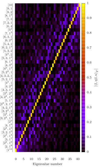
Figure 10: Overlap matrix between the numerically obtained eigenstates $\ket{l,n}_{F}$ of the fermionic model [Eq. (11)] and the non-interacting particle-hole states labelled by the partition $\eta$ shown on the $y$ axis. On the $x$ axis, the states are ordered by increasing $n$. The partitions $\eta$ on the $y$ axis have been ordered in the same way as in Fig.9. Note how this choice leads to the largest overlap being on the main diagonal.

Appendix D Monte Carlo calculation of the matrix elements of the spectral function

In this last Appendix D we briefly describe how the matrix elements appearing in the SF Eq. (33) can be written in a way which is amenable of Monte Carlo sampling. We expand the annihilation operators at angular momentum $\Delta l=(N-1)/\nu-l$ as

$$\hat{a}_{\Delta l}=\int dz_{1}\Phi_{\Delta l}^{*}(z_{1})\hat{\psi}(z_{1}),$$ (45)

where $\Phi_{\Delta l}(z_{1})$ are the single-particle lowest Landau level orbitals in the circular gauge $\Phi_{\Delta l}(z_{1})=\left(z_{1}/\sqrt{2}\right)^{\Delta l}\exp(-|z_{1}|^{2}/4)/\sqrt{2\pi\Delta l!}$. We then write the matrix elements explicitly in first quantization language as

$$\bra{f}\hat{a}_{\Delta l}\ket{0}=\\ =\sqrt{N}\int\Phi_{\Delta l}(z_{1})^{*}\frac{{\Psi_{f}^{[N-1]}}(z^{\prime})^{*}}{\mathcal{N}_{f}}\frac{\Psi_{0}^{[N]}(z)}{\mathcal{N}_{0}}\,\mathcal{D}z$$ (46)

where $z$ is a shorthand for the the particle coordinates $z=\{z_{1},\ldots,z_{N}\}$ and $z^{\prime}$ a shorthand for all the particle coordinates exception made for $z_{1}$, $z^{\prime}=\{z_{2},\ldots,z_{N}\}$, and we define the normalization factors as

$$\mathcal{N}_{0}=\left[\int\mathcal{D}z\,\left|\Psi_{0}^{[N]}(z)\right|^{2}\right]^{1/2}$$ (47)

and

$$\mathcal{N}_{f}=\left[\int\mathcal{D}z^{\prime}\,\left|\Psi_{f}^{[N-1]}(z^{\prime})\right|^{2}\right]^{1/2}.$$ (48)

The final states $\Psi_{f}$ are expanded as power-sum symmetric polynomials multiplying a $(N-1)$-particles Laughlin wavefunction $\Psi_{L}^{[N-1]}(z^{\prime})$. We find that the Monte Carlo sampling of the integrals is strongly facilitated by introducing the probability distribution function

$$\mathcal{P}(z)=\frac{|\Psi_{0}^{[N]}(z_{1}\ldots z_{N})\Psi_{0}^{[N-1]}(z_{2}\ldots z_{N})|}{\int|\Psi_{0}^{[N]}(z_{1}\ldots z_{N})\Psi_{0}^{[N-1]}(z_{2}\ldots z_{N})|\mathcal{D}z}$$ (49)

since in this way we have zeros of the correct order at each particle’s position, which makes the sampling more effective. The obvious disadvantage is that, since not all the coordinates are treated on an equal footing, the relevant matrix element which needs to be sampled [Eq. (46)] cannot be symmetrized over all the coordinates: we however empirically find the usage of Eq. (49) to be a compromise worth the additional computational price.

References

- Jain (2007) J. K. Jain, Composite Fermions (Cambridge University Press, 2007).
- Prange et al. (2012) R. Prange, M. Cage, K. Klitzing, S. Girvin, A. Chang, F. Duncan, M. Haldane, R. Laughlin, A. Pruisken, and D. Thouless, The Quantum Hall Effect, Graduate Texts in Contemporary Physics (Springer New York, 2012), ISBN 9781461233503, URL https://books.google.it/books?id=mxrSBwAAQBAJ.
- Wen (2019) X.-G. Wen, Science 363, eaal3099 (2019), eprint https://www.science.org/doi/pdf/10.1126/science.aal3099, URL https://www.science.org/doi/abs/10.1126/science.aal3099.
- Tsui et al. (1982) D. C. Tsui, H. L. Stormer, and A. C. Gossard, Phys. Rev. Lett. 48, 1559 (1982), URL https://link.aps.org/doi/10.1103/PhysRevLett.48.1559.
- Laughlin (1983) R. B. Laughlin, Phys. Rev. Lett. 50, 1395 (1983), URL https://link.aps.org/doi/10.1103/PhysRevLett.50.1395.
- Arovas et al. (1984) D. Arovas, J. R. Schrieffer, and F. Wilczek, Phys. Rev. Lett. 53, 722 (1984), URL https://link.aps.org/doi/10.1103/PhysRevLett.53.722.
- Nayak et al. (2008) C. Nayak, S. H. Simon, A. Stern, M. Freedman, and S. D. Sarma, Reviews of Modern Physics 80, 1083 (2008), URL https://doi.org/10.1103%2Frevmodphys.80.1083.
- Wen (1990a) X. G. Wen, Phys. Rev. Lett. 64, 2206 (1990a), URL https://link.aps.org/doi/10.1103/PhysRevLett.64.2206.
- Wen (1990b) X. G. Wen, Phys. Rev. B 41, 12838 (1990b), URL https://link.aps.org/doi/10.1103/PhysRevB.41.12838.
- Wen (1991a) X. G. Wen, Phys. Rev. B 43, 11025 (1991a), URL https://link.aps.org/doi/10.1103/PhysRevB.43.11025.
- Wen (1995) X.-G. Wen, Adv. Phys. 44, 405 (1995), eprint cond-mat/9506066.
- Wen (1992) X.-G. Wen, International Journal of Modern Physics B 06, 1711 (1992).
- Chang (2003) A. M. Chang, Rev. Mod. Phys. 75, 1449 (2003), URL https://link.aps.org/doi/10.1103/RevModPhys.75.1449.
- de-Picciotto et al. (1997) R. de-Picciotto, M. Reznikov, M. Heiblum, V. Umansky, G. Bunin, and D. Mahalu, Nature (London) 389, 162 (1997).
- Chang et al. (1996) A. M. Chang, L. N. Pfeiffer, and K. W. West, Phys. Rev. Lett. 77, 2538 (1996), URL https://link.aps.org/doi/10.1103/PhysRevLett.77.2538.
- Banerjee et al. (2018) M. Banerjee, M. Heiblum, V. Umansky, D. E. Feldman, Y. Oreg, and A. Stern, Nature (London) 559, 205 (2018), eprint 1710.00492.
- Aharon Melcer et al. (2023) R. Aharon Melcer, S. Konyzheva, M. Heiblum, and V. Umansky, Nature Physics (2023), ISSN 1745-2481.
- Nakamura et al. (2020) J. Nakamura, S. Liang, G. C. Gardner, and M. J. Manfra, Nature Physics 16, 931 (2020), eprint 2006.14115.
- Bartolomei et al. (2020) H. Bartolomei, M. Kumar, R. Bisognin, A. Marguerite, J. M. Berroir, E. Bocquillon, B. Plaçais, A. Cavanna, Q. Dong, U. Gennser, et al., Science 368, 173 (2020), eprint 2006.13157.
- Cooper (2008) N. Cooper, Advances in Physics 57, 539 (2008), URL https://doi.org/10.1080%2F00018730802564122.
- Bloch et al. (2008) I. Bloch, J. Dalibard, and W. Zwerger, Rev. Mod. Phys. 80, 885 (2008), URL https://link.aps.org/doi/10.1103/RevModPhys.80.885.
- Cooper et al. (2019) N. R. Cooper, J. Dalibard, and I. B. Spielman, Rev. Mod. Phys. 91, 015005 (2019), URL https://link.aps.org/doi/10.1103/RevModPhys.91.015005.
- Goldman et al. (2014) N. Goldman, G. Juzeliū nas, P. Öhberg, and I. B. Spielman, Reports on Progress in Physics 77, 126401 (2014), URL https://doi.org/10.1088%2F0034-4885%2F77%2F12%2F126401.
- Carusotto et al. (2020) I. Carusotto, A. Houck, A. Kollár, P. Roushan, D. Schuster, and J. Simon, Nature Physics 16, 268 (2020), ISSN 1745-2473.
- Carusotto and Ciuti (2013) I. Carusotto and C. Ciuti, Rev. Mod. Phys. 85, 299 (2013), URL https://link.aps.org/doi/10.1103/RevModPhys.85.299.
- Ozawa et al. (2019) T. Ozawa, H. M. Price, A. Amo, N. Goldman, M. Hafezi, L. Lu, M. C. Rechtsman, D. Schuster, J. Simon, O. Zilberberg, et al., Rev. Mod. Phys. 91, 015006 (2019), URL https://link.aps.org/doi/10.1103/RevModPhys.91.015006.
- Gemelke et al. (2010) N. Gemelke, E. Sarajlic, and S. Chu, Rotating few-body atomic systems in the fractional quantum hall regime (2010), URL https://arxiv.org/abs/1007.2677.
- Fletcher et al. (2021) R. J. Fletcher, A. Shaffer, C. C. Wilson, P. B. Patel, Z. Yan, V. Cré pel, B. Mukherjee, and M. W. Zwierlein, Science 372, 1318 (2021), URL https://doi.org/10.1126%2Fscience.aba7202.
- Tai et al. (2017) M. E. Tai, A. Lukin, M. Rispoli, R. Schittko, T. Menke, Dan Borgnia, P. M. Preiss, F. Grusdt, A. M. Kaufman, and M. Greiner, Nature (London) 546, 519 (2017), eprint 1612.05631.
- Léonard et al. (2022) J. Léonard, S. Kim, J. Kwan, P. Segura, F. Grusdt, C. Repellin, N. Goldman, and M. Greiner (2022), URL https://arxiv.org/abs/2210.10919.
- Schine et al. (2016) N. Schine, A. Ryou, A. Gromov, A. Sommer, and J. Simon, Nature (London) 534, 671 (2016), eprint 1511.07381.
- Clark et al. (2020) L. W. Clark, N. Schine, C. Baum, N. Jia, and J. Simon, Nature (London) 582, 41 (2020), eprint 1907.05872.
- Roushan et al. (2017) P. Roushan, C. Neill, A. Megrant, Y. Chen, R. Babbush, R. Barends, B. Campbell, Z. Chen, B. Chiaro, A. Dunsworth, et al., Nature Physics 13, 146 (2017), eprint 1606.00077.
- Kamiyama et al. (2022) A. Kamiyama, M. Matsuura, J. N. Moore, T. Mano, N. Shibata, and G. Yusa, Physical Review Research 4, L012040 (2022), eprint 2201.10180.
- Ashoori et al. (1992) R. C. Ashoori, H. L. Stormer, L. N. Pfeiffer, K. W. Baldwin, and K. West, Phys. Rev. B 45, 3894 (1992).
- Gauthier et al. (2016) G. Gauthier, I. Lenton, N. M. Parry, M. Baker, M. Davis, H. Rubinsztein-Dunlop, and T. Neely, Optica 3, 1136 (2016).
- Gross and Bakr (2021) C. Gross and W. S. Bakr, Nature Physics 17, 1316 (2021).
- Nardin and Carusotto (2020) A. Nardin and I. Carusotto, Europhysics Letters 132, 10002 (2020), URL https://dx.doi.org/10.1209/0295-5075/132/10002.
- Nardin and Carusotto (2023) A. Nardin and I. Carusotto, Phys. Rev. A 107, 033320 (2023), URL https://link.aps.org/doi/10.1103/PhysRevA.107.033320.
- Halperin and Jain (2020) B. I. Halperin and J. K. Jain, Fractional Quantum Hall Effects (WORLD SCIENTIFIC, 2020), URL https://doi.org/10.1142%2F11751.
- Wilkin et al. (1998) N. K. Wilkin, J. M. F. Gunn, and R. A. Smith, Phys. Rev. Lett. 80, 2265 (1998), URL https://link.aps.org/doi/10.1103/PhysRevLett.80.2265.
- Haldane (1983) F. D. M. Haldane, Phys. Rev. Lett. 51, 605 (1983), URL https://link.aps.org/doi/10.1103/PhysRevLett.51.605.
- Trugman and Kivelson (1985) S. A. Trugman and S. Kivelson, Phys. Rev. B 31, 5280 (1985), URL https://link.aps.org/doi/10.1103/PhysRevB.31.5280.
- Simon et al. (2007a) S. H. Simon, E. H. Rezayi, and N. R. Cooper, Phys. Rev. B 75, 075318 (2007a), URL https://link.aps.org/doi/10.1103/PhysRevB.75.075318.
- Simon et al. (2007b) S. H. Simon, E. H. Rezayi, and N. R. Cooper, Phys. Rev. B 75, 195306 (2007b), URL https://link.aps.org/doi/10.1103/PhysRevB.75.195306.
- Cazalilla (2003) M. A. Cazalilla, Phys. Rev. A 67, 063613 (2003), URL https://link.aps.org/doi/10.1103/PhysRevA.67.063613.
- Girvin et al. (1986a) S. M. Girvin, A. H. MacDonald, and P. M. Platzman, Phys. Rev. B 33, 2481 (1986a), URL https://link.aps.org/doi/10.1103/PhysRevB.33.2481.
- Stone (1990) M. Stone, Phys. Rev. B 42, 8399 (1990), URL https://link.aps.org/doi/10.1103/PhysRevB.42.8399.
- Avron et al. (1995) J. E. Avron, R. Seiler, and P. G. Zograf, Phys. Rev. Lett. 75, 697 (1995), URL https://link.aps.org/doi/10.1103/PhysRevLett.75.697.
- Girvin et al. (1986b) S. M. Girvin, A. H. MacDonald, and P. M. Platzman, Phys. Rev. B 33, 2481 (1986b), URL https://link.aps.org/doi/10.1103/PhysRevB.33.2481.
- Yang (2003) K. Yang, Phys. Rev. Lett. 91, 036802 (2003), URL https://link.aps.org/doi/10.1103/PhysRevLett.91.036802.
- Fern et al. (2018) R. Fern, R. Bondesan, and S. H. Simon, Phys. Rev. B 98, 155321 (2018), URL https://link.aps.org/doi/10.1103/PhysRevB.98.155321.
- Imambekov and Glazman (2009) A. Imambekov and L. I. Glazman, Science 323, 228 (2009), URL https://doi.org/10.1126%2Fscience.1165403.
- Imambekov et al. (2012) A. Imambekov, T. L. Schmidt, and L. I. Glazman, Rev. Mod. Phys. 84, 1253 (2012), URL https://link.aps.org/doi/10.1103/RevModPhys.84.1253.
- Haldane (1981) F. D. M. Haldane, Journal of Physics C: Solid State Physics 14, 2585 (1981), URL https://dx.doi.org/10.1088/0022-3719/14/19/010.
- Giamarchi and Press (2004) T. Giamarchi and O. U. Press, Quantum Physics in One Dimension, International Series of Monographs on Physics (Clarendon Press, 2004), ISBN 9780198525004, URL https://books.google.it/books?id=1MwTDAAAQBAJ.
- Stone et al. (1992) M. Stone, H. W. Wyld, and R. L. Schult, Phys. Rev. B 45, 14156 (1992), URL https://link.aps.org/doi/10.1103/PhysRevB.45.14156.
- Wan et al. (2003) X. Wan, E. H. Rezayi, and K. Yang, Phys. Rev. B 68, 125307 (2003), URL https://link.aps.org/doi/10.1103/PhysRevB.68.125307.
- Wan et al. (2008) X. Wan, Z.-X. Hu, E. H. Rezayi, and K. Yang, Phys. Rev. B 77, 165316 (2008), URL https://link.aps.org/doi/10.1103/PhysRevB.77.165316.
- Jolad and Jain (2009) S. Jolad and J. K. Jain, Phys. Rev. Lett. 102, 116801 (2009), URL https://link.aps.org/doi/10.1103/PhysRevLett.102.116801.
- Jolad et al. (2010) S. Jolad, D. Sen, and J. K. Jain, Phys. Rev. B 82, 075315 (2010), URL https://link.aps.org/doi/10.1103/PhysRevB.82.075315.
- Fabbri et al. (2015) N. Fabbri, M. Panfil, D. Clément, L. Fallani, M. Inguscio, C. Fort, and J.-S. Caux, Phys. Rev. A 91, 043617 (2015), URL https://link.aps.org/doi/10.1103/PhysRevA.91.043617.
- Price and Lamacraft (2014) T. Price and A. Lamacraft, Phys. Rev. B 90, 241415 (2014), URL https://link.aps.org/doi/10.1103/PhysRevB.90.241415.
- Price and Lamacraft (2015) T. Price and A. Lamacraft, Quantum hydrodynamics in one dimension beyond the luttinger liquid (2015), URL https://arxiv.org/abs/1509.08332.
- Pustilnik et al. (2006) M. Pustilnik, M. Khodas, A. Kamenev, and L. I. Glazman, Phys. Rev. Lett. 96, 196405 (2006), URL https://link.aps.org/doi/10.1103/PhysRevLett.96.196405.
- Khodas et al. (2007) M. Khodas, M. Pustilnik, A. Kamenev, and L. I. Glazman, Phys. Rev. B 76, 155402 (2007), URL https://link.aps.org/doi/10.1103/PhysRevB.76.155402.
- Macaluso and Carusotto (2017) E. Macaluso and I. Carusotto, Phys. Rev. A 96, 043607 (2017), URL https://link.aps.org/doi/10.1103/PhysRevA.96.043607.
- Macaluso and Carusotto (2018) E. Macaluso and I. Carusotto, Phys. Rev. A 98, 013605 (2018), URL https://link.aps.org/doi/10.1103/PhysRevA.98.013605.
- Bernevig and Haldane (2008) B. A. Bernevig and F. D. M. Haldane, Phys. Rev. Lett. 100, 246802 (2008), URL https://link.aps.org/doi/10.1103/PhysRevLett.100.246802.
- Wen (1991b) X.-G. Wen, Phys. Rev. B 44, 5708 (1991b), URL https://link.aps.org/doi/10.1103/PhysRevB.44.5708.
- Cooper and Simon (2015) N. R. Cooper and S. H. Simon, Phys. Rev. Lett. 114, 106802 (2015), URL https://link.aps.org/doi/10.1103/PhysRevLett.114.106802.
- Umucal ılar and Carusotto (2017) R. O. Umucal ılar and I. Carusotto, Phys. Rev. A 96, 053808 (2017), URL https://link.aps.org/doi/10.1103/PhysRevA.96.053808.
- Palacios and MacDonald (1996) J. J. Palacios and A. H. MacDonald, Phys. Rev. Lett. 76, 118 (1996), URL https://link.aps.org/doi/10.1103/PhysRevLett.76.118.
- Jolad et al. (2007) S. Jolad, C.-C. Chang, and J. K. Jain, Phys. Rev. B 75, 165306 (2007), URL https://link.aps.org/doi/10.1103/PhysRevB.75.165306.
- Haldane (1991) F. D. M. Haldane, Phys. Rev. Lett. 67, 937 (1991), URL https://link.aps.org/doi/10.1103/PhysRevLett.67.937.
- Bettelheim et al. (2006) E. Bettelheim, A. G. Abanov, and P. Wiegmann, Phys. Rev. Lett. 97, 246401 (2006), URL https://link.aps.org/doi/10.1103/PhysRevLett.97.246401.
- Wiegmann (2012) P. Wiegmann, Phys. Rev. Lett. 108, 206810 (2012), URL https://link.aps.org/doi/10.1103/PhysRevLett.108.206810.
- Moore and Read (1991) G. Moore and N. Read, Nuclear Physics B 360, 362 (1991).
- Metropolis and Ulam (1949) N. Metropolis and S. Ulam, Journal of the American Statistical Association 44, 335 (1949), pMID: 18139350, eprint https://www.tandfonline.com/doi/pdf/10.1080/01621459.1949.10483310, URL https://www.tandfonline.com/doi/abs/10.1080/01621459.1949.10483310.
- Metropolis et al. (1953) N. Metropolis, A. W. Rosenbluth, M. N. Rosenbluth, A. H. Teller, and E. Teller, The Journal of Chemical Physics 21, 1087 (1953), eprint https://doi.org/10.1063/1.1699114, URL https://doi.org/10.1063/1.1699114.
- Hastings (1970) W. K. Hastings, Biometrika 57, 97 (1970), ISSN 00063444, URL http://www.jstor.org/stable/2334940.
- Lee et al. (2014) K. H. Lee, Z.-X. Hu, and X. Wan, Phys. Rev. B 89, 165124 (2014), URL https://link.aps.org/doi/10.1103/PhysRevB.89.165124.