Sedimentation of spheroids in Newtonian fluids with spatially varying viscosity

Abstract

This paper examines the rigid body motion of a spheroid sedimenting in a Newtonian fluid with a spatially varying viscosity field. The fluid is at zero Reynolds number, and the viscosity varies linearly in space in an arbitrary direction with respect to the external force. First, we obtain the correction to the spheroid’s rigid body motion in the limit of small viscosity gradients, using a perturbation expansion combined with the reciprocal theorem. Next, we determine the general form of the particle’s mobility tensor relating its rigid body motion to an external force and torque. The viscosity gradient does not alter the force/translation and torque/rotation relationships, but introduces new force/rotation and torque/translation couplings that are determined for a wide range of particle aspect ratios. Finally, we discuss results for the spheroid’s rotation and center-of-mass trajectory during sedimentation. Depending on the viscosity gradient direction and particle shape, a steady orientation may arise at long times or the particle may tumble continuously. These results are significantly different than when no viscosity gradient is present, where the particle stays at its initial orientation for all times. The particle’s center of mass trajectory can also be altered depending on the particle’s orientation behavior –- for example giving rise to diagonal motion or zig-zagging motion. We summarize the observations for prolate and oblate spheroids for different viscosity gradient directions and provide phase plots delineating different dynamical regimes. We also provide guidelines to extend the analysis when the viscosity gradient exhibits a more complicated spatial behavior.

1 Introduction

Fluids with inhomogeneous viscosity fields are ubiquitous around us. For example, certain biological fluids like mucus and extracellular microbial polymers are mixtures of fluids with different viscosities (Howard Berg, 2004), and therefore exhibit variable viscosity, either with (Esparza López et al., 2021) or without sharp viscosity gradients (Du et al., 2012). Similarly, gradients in temperature, salinity, or concentration may induce spatial variation in viscosity, most commonly observed in marine ecosystems (Arrigo et al., 1999). Finally, suspensions of particles in Newtonian fluids (both active and passive) may be treated at the continuum level as fluids with viscosity varying with local volume fraction (Rafaï et al., 2010; Hatwalne et al., 2004).

In this manuscript, we will examine an idealized problem of a single spheroid sedimenting in a spatially varying viscosity field. We will discuss the dynamics that are observed, and how they differ from other situations studied in the literature. By now, it is well-known that in Stokes flow, a spheroid in gravity does not change its orientation due to the particle symmetry and the reversibility of the Stokes equations. If the orientation starts out neither parallel or perpendicular to the gravity direction, the particle will move in a straight diagonal line, the direction of which is determined by the resistances parallel and perpendicular to the particle’s orientation vector (Fig. 1a). These dynamics will change only when symmetry breaking is present in the system. One way in which symmetry breaking occurs is if fluid inertia is present (Cox, 1965; Khayat & Cox, 1989; Auguste et al., 2013), or if the suspending fluid has normal stresses due to the presence of polymers (Kim, 1986; Galdi, 2000; Galdi et al., 2011). For example, small fluid inertia generates a torque that orients the spheroid’s longest axis perpendicular to the external force – the so-called “broad side on” configuration (Dabade et al., 2015). Conversely, fluid viscoelasticity orients the spheroid such that its longest axis is along the force direction – i.e., an “edge wise” configuration (Dabade et al., 2015; Kim, 1986). These effects markedly change the particle trajectory as well as the sedimentation speed (Fig. 1), since the particle’s drag coefficient is a function of orientation and is minimized when the longest axis is along the force direction.

Figure 1: Illustration of spheroid orientation and trajectory during sedimentation in (a) Stokes flow (zero Reynolds number), (b) fluid with finite inertia, and (c) polymeric fluid with normal stresses (large Elasticity number). This paper investigates the behavior when viscosity stratification is present – i.e., case (d)

Another way in which symmetry breaking could occur is if there is a stratified fluid – i.e., variations in density, viscosity, or other fluid properties that alter the force and torque on the particle (More & Ardekani, 2022). This area of research is relatively modern, and most of the efforts have examined the effect of density stratification on particle dynamics (Doostmohammadi et al., 2014; Ardekani et al., 2017). When density increases along the gravity direction, it is found that the drag on a sphere is enhanced as confirmed by theory (Mehaddi et al., 2018), experiments (YICK et al., 2009; Lofquist & Purtell, 1984) and simulations (Hanazaki et al., 2009; More et al., 2021). The buoyancy force also leads to continuous deceleration and absence of a terminal velocity (Doostmohammadi et al., 2014). For anisotropic particles like spheroids, there has been some research to understand their settling behavior in density stratified fluids. Using a reciprocal theorem based approach, Varanasi and Subramanian (Varanasi & Subramanian, 2022) showed that the hydrostatic torque due to buoyancy originating from density stratification tends to rotate the particle in a broad side on configuration (similar to inertia), which had earlier been also shown by Dandekar et al (Dandekar et al., 2020). In the cited papers, it was assumed that the fluid density is not altered by the presence of the particle, and gives rise to a so-called “hydrostatic torque”. However, the particle itself can alter the density field, and this additional effect can modify the particle torque (Varanasi & Subramanian, 2022; More et al., 2021). For example, density is often linked to a scalar field like temperature, which depends on a convection-diffusion equation. Depending on the Peclet number, the density around the particle may or may not be coupled with the fluid flow. In the low Peclet number limit, this additional torque is opposite the hydrostatic torque (Varanasi & Subramanian, 2022; More et al., 2021).

Despite the advances in understanding microhydrodynamics of particles in density stratified fluids, there is a relative lack of literature examining viscosity stratified fluids, even though there is recent evidence suggesting that these effects would be more important than those due to variations in density in a variety of applications (Dandekar & Ardekani, 2020; Jacquemin et al., 2006). For example, viscosity gradients are present in the swimming of micro-organisms, and it is of much interest to biologists to understand how organisms move in such complex environments (Hatwalne et al., 2004; Liebchen et al., 2018; Rafaï et al., 2010; Sokolov & Aranson, 2009), as well as roboticists who design microrobots in such fluids (Zhuang et al., 2017; Nelson et al., 2010; Kim et al., 2016; Palagi et al., 2013; Asghar et al., 2020; Li et al., 2017). Some questions that arise are: how does a spatially varying fluid viscosity affect the common swimming speed, propulsion, and efficiency (Gagnon & Arratia, 2016)? Do microswimmers orient themselves in preferable positions in response to the viscosity gradients (Takabe et al., 2017)? The common approach is to leverage a prototypical swimmer model (squirmers (Shaik & Elfring, 2021; Datt & Elfring, 2019), swimming sheet (Dandekar & Ardekani, 2020; Eastham & Shoele, 2020), Purcell’s swimmer (Qin & Pak, 2023), cilia (Asghar et al., 2020; Palagi et al., 2013)) and then couple it to the Stokes flow field with a variable viscosity. Currently, work has been performed on the the motion of a single sphere in a viscosity varying fluid (Datt & Elfring, 2019), but the effect of particle shape has yet to be considered. We note that the authors in the cited paper found that viscosity gradients give rise to force/rotation and torque/translation coupling for the sphere’s motion, which would otherwise not exist if the viscosity gradient were absent. This type of coupling is likely to give rise to unique rotational dynamics for orientable particles, which we will investigate in this paper.

With this motivation in mind, this manuscript will examine a problem of a single spheroid sedimenting in a Newtonian fluid with a spatially varying viscosity field. The viscosity field varies linearly in space, and its gradient points in an arbitrary direction with respect to the direction of sedimentation (external force). Sec. 2 outlines the particle geometry and equations of motion. Sec. 3 numerically solves for the particle’s rigid body motion in the limit of weak viscosity gradient using the reciprocal theorem. Sec. 4 uses the principles of symmetry to obtain a general expression for the particle mobility tensor relating the particle’s rigid body motion with the force and torque on the spheroid. The force/translation and torque/rotation relationships are unaltered due to the presence of a viscosity gradient, but the viscosity gradient gives rise to new force/rotation and torque/translation coupling terms that depend on three undetermined coefficients. We determine the values of these coefficients numerically, and thus are able to solve the rigid body problem for arbitrary set of forcing, viscosity gradient direction, and particle geometry. Sec. 5 discusses some illustrative examples, wherein the orientations and trajectories of settling spheroids are analysed for different directions of the viscosity gradient. We find that depending on the viscosity gradient direction, particle shape (prolate vs. oblate spheroid), and particle aspect ratio, the spheroid can take on different steady orientation angles, and sometimes experience no steady orientation. The section concludes on how to extend the analysis to more complicated situations, followed by Sec. 6 which summarizes all results.

We note that although this work primarily focuses on passive particles in viscosity stratified fluids, the results here will likely be important in a variety of contexts beyond this work. For example, scientists are interested in quantifying the swimming of particles in viscosity varying fluids, and the mobility relationships developed here can be used for such applications. Furthermore, understanding the rotation behavior and velocity field from a single, orientable particle can help understand their far-field hydrodynamic interactions in a dilute suspension, which is important in understanding concentration instabilities that arise in fibrous suspensions (Koch & Shaqfeh, 1989; Herzhaft & Guazzelli, 1999; Butler & Shaqfeh, 2002; Kuusela et al., 2003; Koch & Shaqfeh, 1991; Nicolai et al., 1998; Shin et al., 2006, 2009; Vishnampet & Saintillan, 2012). We will not comment on this point further, noting that the work acts as a stepping stone for these more complicated problems when viscosity gradients are present.

2 Problem Statement

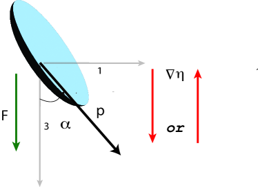
(a) Prolate spheroid

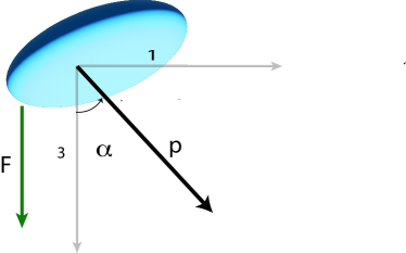
(b) Oblate spheroid

Figure 2: Schematic of a prolate and oblate spheroid falling under an external force acting in the 3-direction. The viscosity gradient is along the 3-direction (parallel or anti-parallel). The particle’s orientation vector $\bm{p}$ makes a polar angle $\alpha\in[0,\pi]$ with respect to the sedimentation direction.

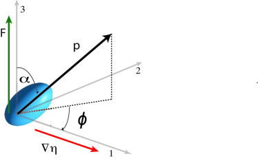
(a) Prolate spheroid

(b) Oblate spheroid

Figure 3: Schematic of a prolate and oblate spheroid falling under an external force $\bm{F}$ acting in the $3$-direction, while the viscosity varies spatially in the $1$-direction. The particle’s orientation $\bm{p}$ makes a polar angle $\alpha\in[0,\pi]$ with respect to the 3-direction, and makes an azimuthal angle $\phi\in[0,2\pi)$ in the 1-2 plane.

2.1 Problem Geometry

The schematic of our system is shown in Figs. 2 and 3. We consider a torque-free spheroid under an external force $\bm{F}$ in a Newtonian fluid with a constant viscosity gradient $\bm{\nabla}\eta$. The force is in the positive 3-direction. The viscosity gradient $\bm{\nabla}\eta$ can be co-linear with the force (Fig. 2, where $\bm{\nabla}\eta$ is in the $\pm$3-direction) or perpendicular to the force (Fig. 3, where $\nabla\eta$ is in the $+$1-direction). The spheroid has three semi-major axes of lengths ($a,b,c$), with $a\neq b=c$. The initial center of mass of the spheroid is $(x_{01},x_{02},x_{03})=(0,0,0)$.

We will define the spheroid’s orientation vector $\bm{p}$ as the direction along its unequal axis (i.e., the $a$-axis). Two different cases arise. A prolate spheroid has $\bm{p}$ along its longest axis, while an oblate spheroid has $\bm{p}$ along its shortest axis. Another way to parameterize the particle shape is through an aspect ratio parameter $A_{R}$ and equivalent radius $R$. Here, $A_{R}$ is the ratio $a/b$, while $R$ is the radius of an equivalent sphere with the same volume.

$$A_{R}=\frac{a}{b}\qquad R=(abc)^{1/3}$$ (1)

The two systems of parameterization are connected by the following relationship:

$$a=RA_{R}^{2/3},\quad b=c=RA_{R}^{-1/3}$$ (2)

Evidently, a prolate particle has its aspect ratio parameter $A_{R}>1$, while an oblate particle has its aspect ratio parameter $A_{R}<1$. Figs.  2 and 3 describe the polar and azimuthal angles $\alpha\in[0,\pi]$ and $\phi\in[0,2\pi)$ for the particle orientation. The next section discusses the equations of motion and the rheology of the fluid.

2.2 Equations of motion and fluid rheology

The fluid surrounding the particle is incompressible and Newtonian. The fluid also has negligible inertia – in other words, the Reynolds number based on the particle’s largest length scale $Re=(\rho_{f}UL_{\text{max}})/\eta_{0}\approx 0$. Here, $\rho_{f}$ is the density of the fluid surrounding the particle, $U$ is the translation speed of the particle, $L_{\text{max}}=max(a,b)$ is the largest axis of the particle, and $\eta_{0}$ is fluid’s viscosity at the origin if the particle were absent.

When these conditions hold, the momentum and mass balance equations in the fluid are given as:

$$\frac{\partial\sigma_{ij}}{\partial x_{j}}=0;\qquad\frac{\partial v_{i}}{\partial x_{i}}=0$$ (3)

where $\sigma_{ij}$ is the stress tensor and $v_{i}$ is the velocity field. Einstein summation convention is assumed – i.e., repeated indices are summed. The stress tensor takes the following form:

$$\sigma_{ij}=-p\delta_{ij}+\eta(\bm{x})\dot{\gamma}_{ij}$$ (4)

where $p$ is the pressure, $\dot{\gamma}_{ij}=\frac{\partial v_{j}}{\partial x_{i}}+\frac{\partial v_{i}}{\partial x_{j}}$ is twice the strain rate tensor and $\eta$ is the viscosity of the medium. In this problem, the viscosity is independent of the strain rate, unlike shear thinning (Anand, 2014; Anand & Christov, 2019b) and viscoelastic (Anand, 2016)fluids, but exhibits a spatial dependence. The viscosity field is:

$$\eta(\bm{x})=\eta_{0}\left(1+\frac{\beta}{R}\bm{\hat{d}}\cdot\bm{x}\right)$$ (5)

In the above equation, $\eta_{0}$ is the viscosity at the origin and $\nabla\eta=\frac{\eta_{0}}{R}\beta\bm{\hat{d}}$ is a constant viscosity gradient with dimensionless magnitude $\beta$ and unit direction $\bm{\hat{d}}$.

The goal of the problem is to solve Eqs. (3), (4), and (5) for the stress and velocity around the particle. The equations have to be solved with the following boundary conditions:

$$v_{i}\rightarrow 0,\qquad|x_{i}|\rightarrow\infty$$ (6a)

$$v_{i}=U_{i}+\epsilon_{ijk}\omega_{j}(x_{k}-x_{k}^{cm}),\qquad x_{i}\in S_{p}$$ (6b)

where $(U_{i},\omega_{i})$ are the rigid body velocities of the particle, $S_{p}$ is the particle surface, $x_{k}^{cm}$ is the center of mass, and $\epsilon_{ijk}$ is the Levi-Civita symbol. An additional constraint is that the particle’s external force and torque are specified. These are:

$$F_{i}=-\int_{S_{p}}\sigma_{ij}n_{j}dS,\quad T_{i}=-\int_{S_{p}}\epsilon_{ikl}(x_{k}-x_{k}^{\text{cm}})\sigma_{lj}n_{j}dS,$$ (7)

where $n_{i}$ is the outward-pointing vector on the particle surface. For this problem, $T_{i}=0$.

In this problem, we specify the viscosity field to have a constant gradient, while for other problems the viscosity field is often found by solving a scalar quantity like temperature or concentration that is a solution to a convection-diffusion equation around the particle. For such problems in the limit of small Peclet number (one-way coupling), the results will be very similar to the problem formulated here, albeit with minor quantitative differences. A more detailed discussion will be provided at the end of the manuscript (Sec. 5.4).

Irrespective of the rheology of the fluid, due to the introduction of the particle, the flow around the particle changes to satisfy the no slip boundary condition on the surface of the particle. The flow , in turn, applies hydrodynamic force (and torque) on the particle, thereby affecting the translation and rotation of the particle, and if the particle is soft, also its deformation. This interaction between the fluid flow and the particle means that the current problem may also be interpreted as a fluid-structure interaction (FSI) problem . FSI problems have already been studied extensively in the case of deformable channels (Anand et al., 2019; Venkatesh et al., 2022)and tubes (Anand & Christov, 2021, 2019a, 2020) conveying Newtonian and non Newtonian fluids in steady as well as transient conditions.

2.3 Non dimensionalization, dimensionless numbers and perturbation expansion

Unless otherwise noted, all quantities from here on out will be written in non-dimensional form. Lengths will be scaled by the average particle size $R$, forces by its magnitude $F$, and viscosities by its value at the origin $\eta_{0}$. Velocities will be scaled by the Newtonian sedimentation velocity $U=\frac{F}{6\pi\eta_{0}R}$ , times by $t_{c}=R/U$, strain rates and rotational velocities by $\dot{\gamma}_{c}=1/t_{c}$, stresses and pressures by $\eta_{0}\dot{\gamma}_{c}$, and torques (if present) by $FR$.

The dynamics of the spheroid will depend on the following dimensionless quantities – the particle aspect ratio parameter $A_{R}$, the particle orientation $\bm{p}$ (characterized by angles $\alpha$ and $\phi$), and the non-dimensional viscosity gradient $\bm{\nabla}\eta$ (characterized by magnitude $\beta$ and direction $\bm{\hat{d}}$):

$$A_{R}=\frac{b}{a};\qquad\bm{p}=[\sin\alpha\cos\phi,\sin\alpha\sin\phi,\cos\alpha];\qquad\nabla\eta=\beta\bm{\hat{d}}$$ (8)

In dimensionless form, the viscosity of the fluid in Figs. 2 and 3 is the following:

$$\eta=1\pm\beta x_{3}\qquad\eta=1+\beta x_{1}$$ (9)

where the first case corresponds to the case where the viscosity gradient is parallel ($+3$ direction) or anti-parallel ($-3$ direction) to the external force, and the second case where the viscosity gradient is perpendicular to the external force. For a general viscosity gradient $\bm{\nabla}\eta$, the particle motion will be a superposition of the solutions for the two cases listed above. We will examine particle dynamics in the limit of small viscosity gradient:

$$Re\ll\beta\ll 1$$ (10)

The above condition indicates that one can neglect fluid inertia and perform a regular perturbation expansion in $\beta$. We will solve for the rigid body motion up to $\mathcal{O}(\beta)$, both numerically and semi-analytically using symmetry arguments listed in the next sections.

3 Numerical solution to particle dynamics

3.1 Reciprocal theorem

We will determine the rigid body motion of the spheroid by performing a perturbation expansion in the non-dimensional viscosity gradient $\beta\ll 1$. We perturb the dependent variables as follows:

$$\begin{split}{\{v_{i},p,\sigma_{ij},\dot{\gamma}_{ij},F_{i},U_{i},\omega_{i}\}}=&\left\{v_{i}^{(0)},p^{(0)},\sigma_{ij}^{(0)},\dot{\gamma}_{ij}^{(0)},F_{i}^{(0)},U_{i}^{(0)},\omega_{i}^{(0)}\right\}\\ &+\beta\left\{u_{i}^{(1)},p^{(1)},\tau_{ij}^{(1)},\dot{\gamma}_{ij}^{(1)},F_{i}^{(1)},U_{i}^{(1)},\omega_{i}^{(1)}\right\}+\ldots\end{split}$$ (11)

and solve for the momentum and mass balances Eqs. (3) - (7) at each order in $\beta$. At leading order, the spheroid sediments in a zero Reynolds number fluid with a constant, non-dimensional viscosity $\eta=1$ and a non-dimensional external force $F=1$:

$$\frac{\partial^{2}v_{i}^{(0)}}{\partial x_{k}\partial x_{k}}-\frac{\partial p^{(0)}}{\partial x_{i}}=0;\qquad\frac{\partial v_{i}^{(0)}}{\partial x_{i}}=0;\qquad F_{i}=\delta_{i3};\qquad T_{i}=0$$ (12)

The solution to the above problem is given in many classical texts (for example see (Kim & Karilla, 2005)). The velocity field is presented in Appendix A, while the rigid body motion satisfies the classical resistance relationship:

$$\left(\begin{array}[]{cc}\bm{R}^{FU}&\bm{R}^{F\omega}\\ \bm{R}^{TU}&\bm{R}^{T\omega}\\ \end{array}\right)\cdot\left(\begin{array}[]{c}\bm{U}^{(0)}\\ \omega^{(0)}\\ \end{array}\right)=\left(\begin{array}[]{c}\bm{F}\\ \bm{T}\\ \end{array}\right)$$ (13)

In this equation, $(\bm{R}^{FU},\bm{R}^{F\omega},\bm{R}^{TU},\bm{R}^{T\omega})$ are the resistance tensors for a spheroid, which are given in Appendix B. The external force and torque are given in Eq. (12) .

At the next order of approximation $\mathcal{O}(\beta)$, the momentum and mass balance equations become Stokes flow with an extra fluid body force $b_{i}$:

$$\frac{\partial^{2}v_{i}^{(1)}}{\partial x_{k}\partial x_{k}}-\frac{\partial p^{(1)}}{\partial x_{i}}+b_{i}=0;\qquad\frac{\partial v_{i}^{(1)}}{\partial x_{i}}=0$$ (14)

Here the body force is due to the spatially varying viscosity field:

$$b_{i}=\frac{\partial\tau_{ij}^{ex}}{\partial x_{j}};\qquad\tau_{ij}^{ex}=(\bm{\hat{d}}\cdot\bm{x})\dot{\gamma}_{ij}^{(0)}$$ (15)

In the above Eq. (15), $\tau_{ij}^{ex}$ is the extra stress tensor, and $\dot{\gamma}^{(0)}_{ij}$ is twice the rate of strain tensor from the leading order velocity field.

We employ the reciprocal theorem to solve for the translational and rotational velocity for the $\mathcal{O}(\beta)$ problem. This theorem has a storied history in the Stokes flow community, as is often used to solve for the rigid body motion of particles in Stokes flow with a fluid body force. The derivation is stated in Appendix C and we present the main results below. In brief, the translational and rotational velocities follow a resistance relationship similar to Eq. (13), except the forces and torques are replaced by an effective polymeric force and torque:

$$\left(\begin{array}[]{cc}\bm{R}^{FU}&\bm{R}^{F\omega}\\ \bm{R}^{TU}&\bm{R}^{T\omega}\\ \end{array}\right)\cdot\left(\begin{array}[]{c}\bm{U}^{(1)}\\ \omega^{(1)}\\ \end{array}\right)=\left(\begin{array}[]{c}\bm{F}^{poly}\\ \bm{T}^{poly}\\ \end{array}\right)$$ (16)

The polymeric force and torque are given as follows:

$$F_{i}^{poly}=-\int_{V_{out}}\frac{\partial v_{ki}^{trans}}{\partial x_{j}}\tau_{kj}^{ex}dV;\qquad T_{i}^{poly}=-\int_{V_{out}}\frac{\partial v_{ki}^{rot}}{\partial x_{j}}\tau_{kj}^{ex}dV$$ (17)

where the integrals are evaluated over the volume $V_{out}$ outside the particle. The quantities $v_{ki}^{trans}$ and $v_{ki}^{trans}$ are the Stokes flow velocity fields around a spheroid in the $k$ direction due to unit translation or unit rotation in the $i$ direction. These quantities are derived from the same velocity fields listed in Appendix A.

3.2 Numerical implementation:

The volume integrals in the Eq. (17) are difficult to evaluate analytically. A custom-made MATLAB code was written to calculate the spheroid’s rigid body motion. This code is similar to the approach used in our prior papers to investigate the motion of ellipsoids in weakly viscoelastic fluids (Wang et al., 2020), except that here the extra stress is modified to account for the viscosity gradient. First, we transform from the laboratory frame to the particle frame of reference where that the origin is at the particle’s center of mass and the Cartesian coordinate axes align with the particle’s principle axes. We then evaluate the volume integrals in Eq. (17) for the polymeric force and torque, using an elliptical coordinate system and performing Gaussian quadrature via Legendre polynomials. We then solve the matrix equations Eq. (13) and Eq. (16) for the rigid body motions at $\mathcal{O}(1)$ and $\mathcal{O}(\beta)$, and transform back to the laboratory frame. The particle’s center of mass and orientation are evolved by solving the rigid body dynamics:

$$\frac{d\bm{x}^{cm}}{dt}=\bm{U};\qquad\quad\frac{d\bm{p}}{dt}=\bm{\omega}\times\bm{p}$$ (18)

We use a forward Euler scheme with $\Delta t=0.01$. More details are found in our prior publications (Wang et al., 2020; Anand & Narsimhan, 2023).

3.2.1 Verification of code

For the case of a sphere sedimenting in a linear, imposed viscosity gradient, we refer to the work by (Datt & Elfring, 2019). Specifically, Eqs.$(7,8)$ in (Datt & Elfring, 2019) are the resistance relationships for the external force $\bm{F}$ and torque $\bm{T}$ on a sphere of radius $a$ in a fluid with a constant viscosity gradient $\bm{\nabla}\eta$, with translational velocity $\bm{U}$ and rotational velocity $\bm{\omega}$. For convenience, these equations are reproduced in dimensional form here:

$$\bm{F}=6\pi a\eta_{0}\bm{U}-2\pi a^{3}\bm{\nabla}\eta\times\bm{\omega}$$

$$\bm{T}=2\pi a^{3}\bm{\nabla}\eta\times\bm{U}+8\pi\eta_{0}a^{3}\bm{\omega}$$

1. Spatial variation in $y$ direction: For a torque-free $(\bm{T}=0)$ sphere sedimenting in the $x$-direction where the dimensional viscosity gradient is along the $y$-direction $\bm{\nabla}\eta=\beta\frac{\eta_{0}}{a}\bm{\hat{y}}$, the above equations give us:

   $$U_{x}=\frac{F_{x}}{\pi a\eta_{0}(6-0.5\beta^{2})};\qquad U_{y}=U_{z}=0$$ (19)

   $$\omega_{x}=\omega_{y}=0\qquad\omega_{z}=0.25\beta\frac{F_{x}}{\pi\eta_{0}a^{2}(6-0.5\beta^{2})}$$ (20)

   The analytical result for $\omega_{z}$ in Eq. (20) is compared against the results of the numerical simulation and the comparison is shown in Fig. 4(a) showing an accurate match.

2. Spatial variation in $x$ direction: Similarly, for a torque-free sphere sedimenting in the $x$-direction where the dimensional viscosity gradient is along the $x$-direction $\bm{\nabla}\eta=\beta\frac{\eta_{0}}{a}\bm{\hat{x}}$, the above equations give:

   $$U_{x}=\frac{F_{x}}{6\pi a\eta_{0}};\qquad U_{y}=U_{z}=0$$ (21)

   $$\omega_{x}=\omega_{y}=\omega_{z}=0$$ (22)

   We compare the results of the simulation against Eq. (21) in Fig 4(b) where a good match is seen.

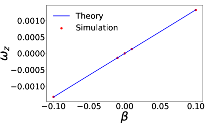
(a) $\bm{F}\propto\bm{\hat{x}}$, $\bm{\nabla}\eta\propto\beta\bm{\hat{y}}$

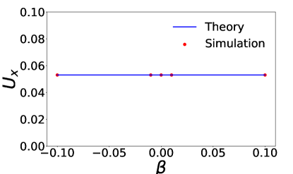
(b) $\bm{F}\propto\bm{\hat{x}}$, $\bm{\nabla}\eta\propto\beta\bm{\hat{x}}$

Figure 4: Code validation for a sphere sedimenting in a fluid with a prescribed viscosity gradient in the (a) $y$-direction and (b) $x$-direction. For all the cases, the external force is a unit vector acting in the $x$-direction, while the external torque is $\bm{T}=0$. The radius and fluid viscosity are $a=1$ and $\eta_{0}=1$, respectively. The results of the theory are from (Datt & Elfring, 2019), expanded in Sec. 3.2.1.

4 Semi analytical theory

4.1 Introduction and motivation

The simulations described in the previous section solve the rigid body motion of the particle, but are computationally intensive. At each timestep, one has to evaluate six volume integrals in Eq. (17) to obtain the polymeric force and torque. Furthermore, a new time sweep has to be performed if one examines a different viscosity gradient direction and magnitude.

An alternative approach to obtain the same dynamics is to develop a semi-analytical theory based on the symmetry of the problem. Such a theory will give the general form of the particle’s motion in terms of three undetermined constants, which in turn can be found by performing simulations at three specific configurations. The result of this analysis is that one can cheaply obtain the particle’s motion for an arbitrary set of particle orientations, forcing, and viscosity gradients.

What we are doing is essentially finding the general form of the mobility tensor when a viscosity gradient is present. Thus, the analysis below will not only give general information about the force-rotation coupling of these orientable particles, but can also give results for the case when a torque is applied – for example, the torque-translation coupling. A description is below.

4.2 General form of mobility tensor

The governing momentum and continuity Eqns. (3) - (7) are linear in the external force and torque $(\bm{F},\bm{T})$. Thus, the translational and rotational velocities $(\bm{U},\bm{\omega})$ are also linear in these quantities and obey the following relationship:

$$\left(\begin{array}[]{c}\bm{U}\\ \omega\\ \end{array}\right)=\left(\begin{array}[]{cc}\bm{A}&\bm{B}\\ \bm{B}^{T}&\bm{D}\\ \end{array}\right)\cdot\left(\begin{array}[]{c}\bm{F}\\ \bm{T}\\ \end{array}\right)$$ (23)

Here, $(\bm{A},\bm{B},\bm{D})$ are mobility tensors that are non-dimensionalized by $\left(\frac{U}{F},\frac{U}{FR},\frac{U}{FR^{2}}\right)=\left(\frac{1}{6\pi\eta_{0}R},\frac{1}{6\pi\eta_{0}R^{2}},\frac{1}{6\pi\eta_{0}R^{3}}\right)$, respectively . In a constant viscosity fluid, these tensors are only a function of the particle shape and orientation, characterised by the aspect ratio parameter $A_{R}$ and the orientation vector $\bm{p}$. If a viscosity gradient is present, the tensors will also be a function of the non-dimensional viscosity gradient $\bm{\nabla}\eta=\beta\bm{\hat{d}}$. Note: the the off-diagonal terms of the matrix in Eq. (23) are transposes of each other as can be proved by the reciprocal theorem (not shown here).

In the limit of $\beta\ll 1$, we expand the mobility tensors in a Taylor series as follows:

$$\left\{{A}_{ij},{B}_{ij},{D}_{ij}\right\}=\left\{{A}^{(0)}_{ij},{B}^{(0)}_{ij},{D}^{(0)}_{ij}\right\}+\beta\left\{{A}^{(1)}_{ij},{B}^{(1)}_{ij},{D}^{(1)}_{ij}\right\}$$ (24)

At leading order ($O(1)$), the tensors are the same as those for the particle in a constant viscosity fluid. These quantities are well-characterized and formulas are given in Appendix B for a general ellipsoid. Specifically, for the case where the particle has an orientation vector $\bm{p}$, they take the form:

$${A}^{(0)}_{ij} =c_{1}\left(\delta_{ij}-{p_{i}}{p_{j}}\right)+c_{2}{p_{i}}{p_{j}}$$ (25a)

$${D}^{(0)}_{ij} =c_{3}\left(\delta_{ij}-{p_{i}}{p_{j}}\right)+c_{4}{p_{i}}{p_{j}}$$ (25b)

$${B}^{(0)}_{ij} =0$$ (25c)

where $c_{1},c_{2},c_{3}$ and $c_{4}$ are functions of the apsect ratio parameter and are given in Appendix B.

At $\mathcal{O}(\beta)$, the motion will be linear in $\bm{\nabla}\eta$. Thus, in non-dimensional form, the mobility tensors take the following structure:

$$A_{ij}^{(1)} =\alpha_{ijk}\hat{d}_{k}$$ (26a)

$$D_{ij}^{(1)} =\beta_{ijk}\hat{d}_{k}$$ (26b)

$$B_{ji}^{(1)} =M_{ikj}\hat{d}_{k}$$ (26c)

where $\hat{d}_{k}$ is the direction of the viscosity gradient. Therefore the problem of finding the mobility matrices $(A_{ij}^{(1)},B_{ij}^{(1)},{D}_{ij}^{(1)})$ reduces to the problem of finding $\alpha_{ijk}$,$\beta_{ijk}$ and $M_{ijk}$. For a spheroid, these third order tensors depend on the orientation product $p_{i}p_{j}$, since fore-aft symmetry dictates that changing $p_{i}$ to $-p_{i}$ will not alter the results. Noting that $(\alpha_{ijk},\beta_{ijk})$ are third order true tensors, and such tensors cannot be formed from $p_{i}p_{j}$, we obtain the result:

$$\alpha_{ijk}=\beta_{ijk}=0$$ (27)

The above relationship means that at $\mathcal{O}(\beta)$, the force-velocity coupling and torque-angular velocity coupling are unchanged. However, as we will see next, the force-rotation coupling and torque-velocity coupling will change. $B_{ji}$ is a pseudo tensor since it connects a pseudo vector (angular velocity) with a true vector (force). Therefore, $M_{ikj}$ is a third order pseudo tensor, which depends on the orientation product $p_{i}p_{j}$. The general form of $M_{ijk}$ is given below as:

$$M_{ijk}=\lambda_{1}\epsilon_{ijk}+\lambda_{2}p_{i}\epsilon_{jkq}p_{q}+\lambda_{3}p_{j}\epsilon_{ikq}p_{q}+\lambda_{4}p_{k}\epsilon_{ijq}p_{q}$$ (28)

where $\lambda_{1},\lambda_{2},\lambda_{3},\lambda_{4}$ are dimensionless coefficients that depend only on the aspect ratio parameter $A_{R}$. One can show that without loss of generality $\lambda_{2}=0$ (see Appendix D) and therefore the problem reduces to finding the coefficients $\lambda_{1},\lambda_{3},\lambda_{4}$. In other words, Eq. (28) reduces to

$$M_{ijk}=\lambda_{1}\epsilon_{ijk}+\lambda_{3}p_{j}\epsilon_{ikq}p_{q}+\lambda_{4}p_{k}\epsilon_{ijq}p_{q}$$ (29)

In summary, the mobility relationships up to $\mathcal{O}(\beta)$ reduce to:

$$U_{i}=A_{ij}^{(0)}F_{j}+\beta M_{jki}\hat{d}_{k}T_{j}$$ (30a)

$$\omega_{i}=\beta M_{ikj}\hat{d}_{k}F_{j}+D_{ij}^{(0)}T_{j}$$ (30b)

where $A_{ij}^{(0)}$,$D_{ij}^{(0)}$ are the known mobility tensors for a spheroid without a viscosity gradient, given by Eq. (25), while $M_{ijk}$ is the cross-coupling term given by Eq. (29). The unknown coefficients for the tensor $M_{ijk}$ are $(\lambda_{1},\lambda_{3},\lambda_{4})$, which are functions of the aspect ratio parameter $A_{R}$ for the spheroid. The next section discusses how we determine these coefficients.

4.3 Determining coefficients $\lambda_{1},\lambda_{3},\lambda_{4}$ for the mobility matrix $M_{ijk}$(force-rotation and torque-translation coupling)

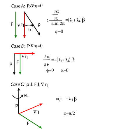
Figure 5: Simulations carried out to estimate the parameters $(\lambda_{1},\lambda_{3},\lambda_{4})$ in the third order pseudo tensor $M_{ijk}$ given by Eq. (29). The orientation angles $(\alpha,\phi)$ are defined in Figs. 2 and 3 respectively.

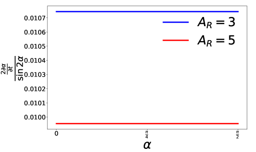
Figure 6: Verification of theory by plotting of Eq. (33) for different values of $\alpha$, for a prolate spheroid with external force $\bm{F}$ and viscosity gradient $\bm{\nabla}\eta$ in the positive $z$-direction. This situation corresponds to Case A shown in Fig. 5a.

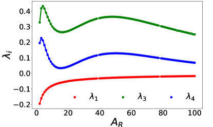
(a) Prolate spheroid

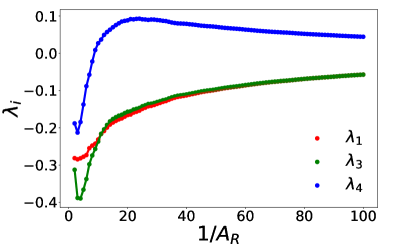
(b) Oblate spheroid

Figure 7: Computed values of $(\lambda_{1},\lambda_{3},\lambda_{4})$ for prolate and oblate spheroids for different values of aspect ratio parameters $A_{R}$.

Fig 5 outlines the simulations we perform to obtain the coefficients $(\lambda_{1},\lambda_{3},\lambda_{4})$ for $M_{ijk}$ in Eq. (29). We examine a torque-free particle $(T_{i}=0)$ and quantify its angular velocity $\omega_{i}$ for the three specific geometries listed below. We note that the angular velocity can cause two effects – it can change the spheroid’s orientation or it can keep the orientation the same but spin it along its axis. The rate of change of the orientation is given by:

$$\frac{dp_{i}}{dt}=\epsilon_{ijk}\omega_{j}p_{k}$$ (31)

while the rate of spinning is:

$$\Omega=\omega_{i}p_{i}$$ (32)

These quantities are computed for the cases below:

1. Case A: $\bm{\nabla}\eta\times\bm{F}=0$: Here, we examine the situation in Fig  5a where the external force and viscosity gradient are in the same direction – i.e., $\bm{F}=\bm{\hat{d}}=\bm{\hat{z}}$. The particle has its orientation in the $x-z$ plane with an angle $\alpha$ with respect to the force direction – i.e., $\bm{p}=[\sin\alpha,0,\cos\alpha]$. Using Eqs. (29), (30b), and (31), one finds the angular velocity to be:

   $$\omega_{2}=-\frac{d\alpha}{dt}=-\frac{1}{2}\beta\left(\lambda_{3}+\lambda_{4}\right)\sin({2\alpha})$$ (33)

   Thus, performing one simulation at a specific polar angle and viscosity gradient magnitude (say $\alpha=\pi/4,\beta=0.1)$ allows us to obtain $(\lambda_{3}+\lambda_{4})$. In Fig 6, we plot simulations of $2\frac{\frac{d\alpha}{dt}}{\sin{2\alpha}}$ for many values of angles $\alpha$ and non-dimensional viscosity gradients $\beta$. This quantity is constant for all values of $\alpha$ and $\beta$, but is a function of the aspect ratio parameter $A_{R}$, which is consistent with the expression listed above.
   

2. Case B: $\bm{\nabla}\eta\cdot\bm{F}=0,\bm{p}\times\bm{F}=0$: We examine the situation in Fig  5b where the external force and viscosity gradient are perpendicular to each other – i.e., $\bm{F}=\bm{\hat{z}}$, $\bm{\hat{d}}=\bm{\hat{x}}$. The particle has its orientation along the force direction – i.e., $\bm{p}=[0,0,1]$ – which corresponds to the polar and azimuthal angles of $\alpha=\phi=0$ in Fig 3. Using Eqs. (29), (30b), and (31), one finds the angular velocity to be:

   $$\omega_{2}=\frac{d\alpha}{dt}|_{\alpha=\phi=0^{\circ}}=-\beta(\lambda_{1}-\lambda_{3}+\lambda_{4})$$ (34)

   Performing one simulation at a specific value of $\beta$ (e.g., $\beta=0.1$) allows us to obtain $(\lambda_{1}-\lambda_{3}+\lambda_{4})$.
   

3. Case C: $\bm{\nabla}\eta\perp\bm{F}\perp\bm{p}$: We examine case in Fig  5c where the orientation, viscosity gradient, and force are all perpendicular to each other – i.e., $\bm{F}=\bm{\hat{z}}$, $\bm{\hat{d}}=\bm{\hat{x}}$, $\bm{p}=\bm{\hat{y}}$. Here, the particle will spin but not change orientation. Using Eqs. (29), (30b), and (32), we find the spinning rate to be:

   $$\Omega=\omega_{2}=-\beta\lambda_{1}$$ (35)

   Performing one simulation at a specific value of $\beta$ (e.g., $\beta=0.1$) allows us to obtain $\lambda_{1}$.
   

The three simulations listed above yield a linear system of equations for the coefficients $(\lambda_{1},\lambda_{3},\lambda_{4})$ that can be solved. Fig 7 shows the values of the coefficients for different values of the aspect ratio parameter $A_{R}$, for both prolate and oblate spheroids. Once these coefficients are tabulated, one has a general form for the rigid body motion (Eq. (30)) for spheroids that can be solved for arbitrary viscosity gradient, orientation, aspect ratio, and external force/torque.

5 Results and illustrative examples

In Sec. 4, we developed a theory to describe the rigid body motion of a spheroid in a spatially varying viscosity field. The general form of the translational and rotational velocities is given in Eq. (30), where $A_{ij}^{(0)}$ and $D_{ij}^{(0)}$ are the standard mobility tensors for force/translation and torque/rotation in Stokes flow, and $M_{ijk}$ is a newly introduced coupling tensor between force/rotation and torque/translation that arises due to viscosity gradients. The tensor $M_{ijk}$ is given in Eq.  (29) in terms of three coefficients $(\lambda_{1},\lambda_{3},\lambda_{4})$ that are only functions of the spheroid aspect ratio parameter $A_{R}$. These coefficients are estimated numerically using the reciprocal theorem (see Sec. 3 and Fig. 7).

In this section, we investigate the spheroid’s dynamics for some special cases and discuss the physics that arise. Details are below.

5.1 Viscosity gradient is along or opposite the force direction

5.1.1 Governing equations

Let us examine the situation in Fig. 2 where the external force is in the positive $z$-direction, and the viscosity gradient is either parallel to the force (positive $z$-direction) or anti-parallel to the force (negative $z$-direction). In this case, the particle orientation only has one degree of freedom, namely the polar angle $\alpha$ measured from the $z$-axis. Without loss of generality, we will state that $\bm{p}$ lies in the $x-z$ plane, and thus $\bm{p}=[\sin\alpha,0,\cos\alpha]$. From our theory (Eqs. (29), (30b), and (31)), the orientation angle obeys the following equation:

$$\frac{d\alpha}{dt}=\pm\frac{1}{2}\beta(\lambda_{3}+\lambda_{4})\sin(2\alpha)$$ (36)

where $\pm$ illustrates the cases where the viscosity gradient is parallel ($+$) or anti-parallel ($-$) to the force. The translational motion of the particle obeys:

$$\frac{dx}{dt}=\frac{1}{2}(c_{2}-c_{1})\sin(2\alpha);\qquad\frac{dz}{dt}=c_{1}\sin^{2}\alpha+c_{2}\cos^{2}\alpha$$ (37)

where $c_{1}$ and $c_{2}$ are the mobility coefficients for spheroid translation in Stokes flow (given in Appendix B in dimensional form). Major conclusions are given below.

5.1.2 Particle takes a stable orientation depending on its shape and viscosity gradient direction

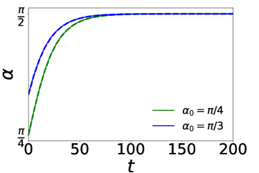
(a) Prolate, parallel

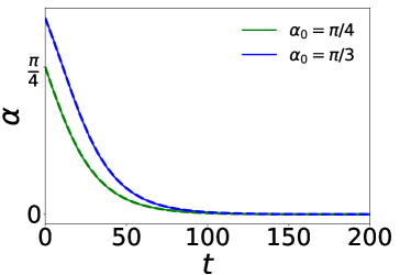
(b) Oblate, parallel

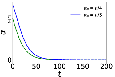
(c) Prolate, anti-parallel

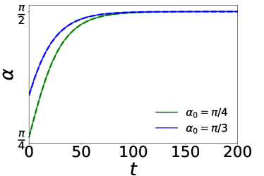
(d) Oblate, anti-parallel

Figure 8: Orientation angle $\alpha$ vs. time for prolate and oblate spheroids when the external force $\bm{F}$ and viscosity gradient $\bm{\nabla}\eta$ are parallel or anti-parallel to each other. The left figures (a,c) correspond to prolate spheroids with $A_{R}=5$, while those the right figures (b,d) correspond to oblate spheroids with $A_{R}=1/5$. The top row (a,b) is the case when the $\bm{F}$ and $\bm{\nabla}\eta$ are in the same direction, while the bottom row (b,d) is the case when they are in opposite directions. The solid curves are from full numerical simulations based on the reciprocal theorem, while the dashed curves are from the reduced order theory (solving Eq. (36)). The dimensionless viscosity gradient is $\beta=0.1$.

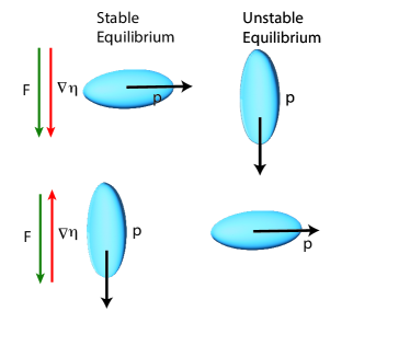
(a) Prolate spheroid

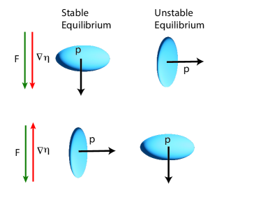
(b) Oblate spheroid

Figure 9: Steady configurations attained by (a) prolate and (b) oblate spheroids when the external force $\bm{F}$ and viscosity gradient $\bm{\nabla}\eta$ are co-linear. The top row is for the case when the external force and the viscosity gradient are in the same direction, while the bottom row is when they are in the opposite direction.

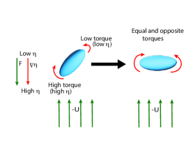
(a) Parallel

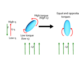
(b) Anti-parallel

Figure 10: Illustration of unequal torques created on a prolate spheroid when the force and viscosity gradient are co-linear. The left figure (a) is when the viscosity gradient and force are in the same direction, while the right figure (b) is when they are in opposite directions.

Fig. 8 plots the evolution of $\alpha$ with respect to time for prolate and oblate spheroids, for the cases when the force $\bm{F}$ and viscosity gradient $\bm{\nabla}\eta$ are parallel and anti-parallel to each other. For each set of conditions, two curves are given – one arising from the reduced order theory (dashed curve, Eq. (36)), and another from full numerical simulations where the reciprocal theorem is used at every time step (solid curve). The overlap is indistinguishable, thereby validating our theory. The second observation we make is that that irrespective of the initial orientation and viscosity gradient direction (parallel or anti parallel), both prolate and oblate spheroids evolve to a steady configuration of $\alpha$. This observation is very different than what is observed in Stokes flow where the orientation stays at its initial angle at all times (Leal, 2007).

Fig. 9 summarizes the steady orientations observed for different particle shapes and viscosity gradient directions. When the external force and the viscosity gradient are parallel to each other, the prolate spheroid adopts a stable configuration where the projector is perpendicular to external force, while the oblate spheroid orients itself such the projector is along the same direction as the external force. In both of these cases, the spheroid (whether prolate or oblate) has its shortest axis oriented along the direction of the viscosity gradient. On the other hand, when the spheroid is falling in the direction of decreasing viscosity (i.e., $\bm{F}$ and $\bm{\nabla}\eta$ are anti-parallel), the prolate spheroid attains a stable configuration where the projector is oriented along the force direction, whilst the oblate spheroid orients the projector perpendicular to the force direction. In both these cases, the longest axis of the particle (whether prolate and oblate) will be along the force direction.

To provide a physical understanding of this behavior, we refer to Fig. 10. Here, as observed from the reference frame of the particle, the flow around the prolate spheroid bifurcates into two parts about the stagnation point and engenders both a clockwise and counter-clockwise hydrodynamic torque. Fig. 10(a) illustrates the magnitude of the torques for the case when the viscosity gradient is in the same direction as the force, while Fig. 10(b) illustrates the case when the viscosity gradient is in the opposite direction. The pictures illustrate that the the unequal torques push the particle toward the stable orientations discussed above.

Lastly, we note that Fig. 9 summarizes the unstable, steady orientations that can occur for different combinations of viscosity gradient and particle shape. These orientations only exist if the initial condition is at a specific angle, and can only be observed in exceptionally rare cases.

5.1.3 Particle translation is different than in Stokes flow

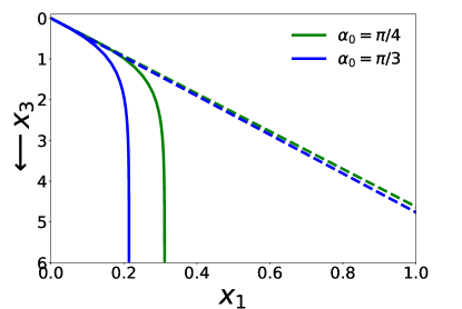
(a) Prolate, $A_{R}=5$

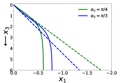
(b) Oblate, $A_{R}=1/5$

Figure 11: Particle trajectories for (a) prolate and (b) oblate spheroids when the external force and viscosity gradient are in the same direction ($\bm{F}=\bm{\hat{z}},\bm{\nabla}\eta=\beta\bm{\hat{z}}$). The dashed curves correspond to when no viscosity gradient is present ($\beta=0$), while the solid curve is when a viscosity gradient is present ($\beta=0.1$). Different color curves correspond to different initial starting angles $\alpha_{0}$. The prolate spheroid has $A_{R}=5$ while the oblate spheroid has $A_{R}=1/5$.

Beyond orientational kinematics, we are also interested in the translation of the spheroid. In a constant viscosity fluid with zero inertia, it is well-known that the particle stays at its initial orientation (Leal, 2007). If the initial angle is $\alpha=0$, $\frac{\pi}{2}$, or $\pi$, the particle will sediment vertically, while if $\alpha$ is not these values, the particle will drift in a straight, diagonal path. The direction in which the particle sediments is dictated by the resistances parallel and perpendicular to its orientation vector $\bm{p}$.

When a viscosity gradient is present, the translational velocity $\bm{U}$ obeys the same differential equation as the Stokes flow case (Eq. (37)), since we found that the viscosity gradient does not alter the force/translation coupling (see Eq. (30)). Thus, on the surface, it appears that the particle trajectory may seem unchanged due to the presence of a spatially varying viscosity field. However, upon closer inspection, we see that the differential equation (Eq. (30)) depends on the particle’s orientation angle $\alpha$, which itself is altered due to the viscosity gradient as discussed in the previous section. Thus, the viscosity gradient plays an indirect role in altering the translational dynamics.

Fig. 11 plots the trajectories of oblate and prolate spheroids for different values of the initial orientation angle $\alpha_{0}$. For $\alpha_{0}\neq 0$, $\frac{\pi}{2}$, and $\pi$, we observe motion in the sedimentation direction (3-direction) as well as a cross stream drift (1-direction). For the case when no viscosity gradient is present, the particle moves in a straight, diagonal path. When a viscosity gradient is present, the trajectory is no longer a straight line. The cross-stream drift eventually stops when the spheroid reaches a stable orientation, beyond which the spheroid sediments vertically in the $3$-direction. Since the spheroid ceases to drift once the stable orientation is reached, a spheroid whose initial orientation is further away from its stable orientation will drift further than a spheroid whose initial orientation is closer to its stable orientation. Therefore, for a prolate spheroid, a particle with initial orientation $\alpha_{0}=\pi/4$ will drift further than one with $\alpha_{0}=\pi/3$, since the stable orientation is $\alpha=\pi/2$ (see Fig. 11(a)). Conversely, for an oblate spheroid, the particle with an initial orientation $\alpha_{0}=\pi/3$ will drift further than one with $\alpha_{0}=\pi/4$, since the stable orientation is at $\alpha=0$.

5.2 Viscosity gradient is perpendicular to the external force

5.2.1 Governing equations

We will now examine the situation in Fig. 3 where the external force is in the positive $z$-direction ($\bm{F}=\bm{\hat{z}}$), and the viscosity gradient is perpendicular to the force ($\bm{\nabla}\eta=\beta\bm{\hat{x}}$). The spheroid’s orientation can point in any direction, and we state it takes the form $\bm{p}=[\sin\alpha\cos\phi,\sin\alpha\sin\phi,\cos\alpha]$, where $\alpha$ and $\phi$ are the polar and azimuthal angles, respectively. From our theory (Eqs. (29), (30b), and (31)), the orientation angles evolve as follows:

$$\frac{d\alpha}{dt}=-\beta\left(\lambda_{1}-\lambda_{3}\sin^{2}\alpha+\lambda_{4}\cos^{2}\alpha\right)\cos\phi$$ (38a)

$$\frac{d\phi}{dt}=\beta(\lambda_{1}+\lambda_{4})\cot\alpha\sin\phi$$ (38b)

where $\lambda_{1},\lambda_{3},$ and $\lambda_{4}$ are the force-rotation mobility coefficients determined in Sec. 4. The translation of the particle obeys the following:

$$\frac{dx}{dt}=\frac{1}{2}(c_{2}-c_{1})\sin(2\alpha)\cos\phi;\qquad\frac{dy}{dt}=\frac{1}{2}(c_{2}-c_{1})\sin(2\alpha)\sin\phi;\qquad\frac{dz}{dt}=c_{1}\sin^{2}\alpha+c_{2}\cos^{2}\alpha$$ (39)

where $c_{1}$ and $c_{2}$ are the mobility coefficients for particle translation in Stokes flow (given in Appendix B in dimensional form). Major conclusions are given below.

5.2.2 Particle can take a steady orientation different than the force and viscosity gradient directions

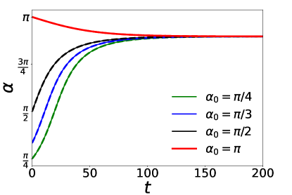
(a) Prolate spheroid

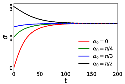
(b) Oblate spheroid

Figure 12: Orientation angle $\alpha$ vs. time for prolate ($A_{R}=5$) and oblate ($A_{R}=1/5$) spheroids when the external force and viscosity gradient are perpendicular ($\bm{F}=\bm{\hat{z}},\bm{\nabla}\eta=\beta\bm{\hat{x}}$). The dimensionless viscosity gradient is $\beta=0.1$, and the particle initially starts in the plane of $\bm{F}$ and $\bm{\nabla}\eta$ (i.e., $\phi_{0}=0$). Solid curves are from full numerical simulations based on the reciprocal theorem, while the dashed curves are from the reduced order theory (solving Eq. (38)).

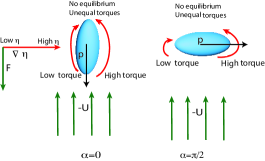
(a) Prolate spheroid

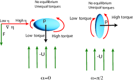
(b) Oblate spheroid

Figure 13: Schematic explaining the absence of steady orientations at $\alpha=0$ and $\alpha=\pi/2$ for (a) prolate and (b) oblate spheroids when the external force and viscosity gradient are perpendicular. This schematic is shown in the particle’s frame of reference.

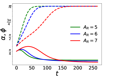
(a) Prolate, $\beta=0.1$

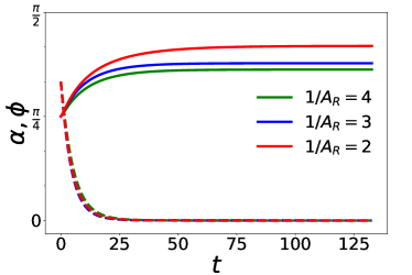
(b) Oblate, $\beta=0.1$

Figure 14: Orientation angles $\alpha(t)$ and $\phi(t)$ for prolate and oblate spheroids when the external force and viscosity gradient are perpendicular ($\bm{F}=\bm{\hat{z}},\bm{\nabla}\eta=\beta\bm{\hat{x}}$). The dashed curves show the evolution of $\phi$, while the solid curves show the evolution of $\alpha$. For all cases, the initial orientation is given by the ordered pair $(\phi_{0},\alpha_{0})=(\pi/3,\pi/4)$ and the dimensionless viscosity gradient is $\beta=0.1$. The results show that $\phi\rightarrow 0$ or $\pi$, and hence the particle becomes co-planar with $\bm{F}$ and $\bm{\nabla}\eta$.

.

We will first discuss the case when the particle starts in the same plane as $\bm{F}$ and $\bm{\nabla}\eta$ – in other words $\phi_{0}=0$. From Eq. (38b), we see that $d\phi/dt=0$ for this angle, so the particle stays at $\phi=0$ and only the polar angle $\alpha$ will change. Fig. 12 plots $\alpha$ versus time for both prolate and oblate spheroids, for the specific case of $A_{R}=5$ and $A_{R}=-1/5$, respectively. First of all, we note that the results from the reduced order theory (solid curve, Eq. (38)) are virtually indistinguishable from the full numerical simulation (dashed curve), indicating the validity of our theory. Secondly, for all starting conditions, we observe the particle converges to one steady orientation. However, this steady orientation is not $\alpha=0$, $\alpha=\pi$, or $\alpha=\pi/2$, which was the case when the force and viscosity gradient vectors were co-linear.

We elucidate this point more clearly in Fig. 13. Here, we observe that neither $\alpha=0,\pi/2,$ or $\pi$ are steady configurations because the counter-clockwise torque is different than the clockwise torque at these specific angles. Some general trends are described below for prolate and oblate particles:

• Prolate spheroids: For prolate spheroids, we observe from Fig. 13 that the difference between the counter-clockwise and clockwise torques is smaller for $\alpha=0$ and $\pi$ (where the long axis is along the force direction) compared to $\alpha=\pi/2$ (where the long axis is along the viscosity gradient direction). Therefore, the steady orientation is closer to $\alpha=0$ and $\pi$ than to $\alpha=\pi/2$, and continues to approach $\alpha=0$ or $\pi$ as the aspect ratio increases. In the limiting case of needle like particles where $A_{R}\to\infty$ the steady orientation reaches $\alpha=n\pi$. Between the two configurations of $\alpha=0+\Delta$ and $\alpha=\pi-\Delta$ (where $\Delta$ is a positive constant depending on aspect ratio), $\alpha=\pi-\Delta$ is the stable configuration, while $\alpha=0+\Delta$ is unstable (see Fig.12(a)).

• Oblate spheroids: For oblate spheroids, the difference in hydrodynamic torques is larger at $\alpha=0$ compared to $\alpha=\pi/2$, because in the former case the longer axis is oriented along the viscosity gradient direction. Therefore, for oblate spheroids, the equilibrium orientation configuration is closer to $\alpha=\pi/2$ than to $\alpha=0$. In the limiting case of a thin disc where $A_{R}\rightarrow 0$, the stable orientation is at $\alpha=\pi/2$. Between the two configurations of $\alpha=\pi/2\pm\xi$ (where $\xi$ is a positive constant depending on the aspect ratio), $\alpha=\pi/2-\xi$ is the stable orientation, while $\alpha=\pi/2+\xi$ is an unstable orientation (see Fig. 12(b))

The results discussed above illustrate the dynamics when the initial particle orientation is co-planar with $\bm{F}$ and $\bm{\nabla}\eta$ – i.e., $\phi_{0}=0$ or $\phi=\pi$. Fig. 14b plots the orientation angles $\phi$ and $\alpha$ over time when the starting angle is no longer co-planar with $\bm{F}$ and $\bm{\nabla}\eta$ – i.e., $\phi_{0}\neq 0$ or $\pi$. We see that at long times, the angle $\phi\rightarrow 0$ or $\pi$ – i.e., the orientation ends up in the same plane as $\bm{F}$ and $\bm{\nabla}\eta$. The angle $\alpha$ also converges to the same result as before. Thus, we conclude that the steady orientation angles discussed previously are stable to out of plane perturbations.

5.2.3 Not all spheroids have a steady orientation

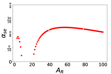
(a) Prolate

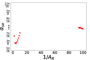
(b) Oblate

Figure 15: Stable orientations $\alpha_{se}$ for prolate and oblate spheroids of different aspect ratio parameters $A_{R}$ when the external force and viscosity gradient are perpendicular to each other ($\bm{F}=\bm{\hat{z}}$ $\bm{\nabla}\eta=\beta\bm{\hat{x}}$, $\beta=0.1$). Regions that do not have data points are regions where the particle tumbles and does not exhibit a stable orientation.

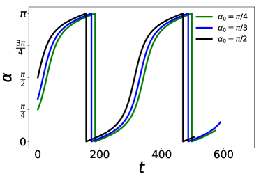
(a) Prolate, $A_{R}=13$

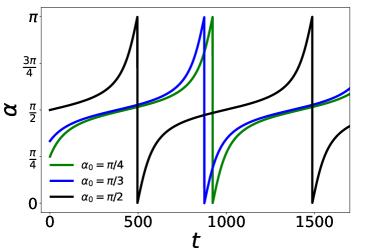
(b) Oblate, $A_{R}=1/13$

Figure 16: Tumbling of (a) prolate spheroids and (b) oblate spheroids when the external force and viscosity gradient are perpendicular to each other ($\bm{F}=\bm{\hat{z}}$ $\bm{\nabla}\eta=\beta\bm{\hat{x}}$, $\beta=0.1$). For the aspect ratio parameter shown in this figure ($A_{R}=13$ for prolate and $A_{R}=1/13$ for oblate), there is no stable orientation and the spheroids continue to tumble.

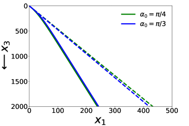
(a) $A_{R}=5$

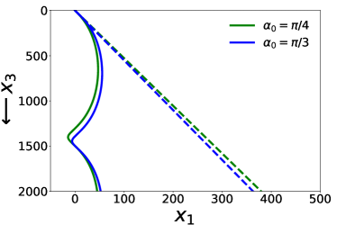
(b) $A_{R}=11$

Figure 17: Particle trajectories for prolate spheroids with (a) $A_{R}=5$ and (b) $A_{R}=11$ when the external force and viscosity gradient are perpendicular ($\bm{F}=\bm{\hat{z}},\bm{\nabla}\eta=\beta\bm{\hat{x}}$). The dashed curves correspond to when no viscosity gradient is present ($\beta=0$), while the solid curve is when a viscosity gradient is present ($\beta=0.1$). Different color curves correspond to different initial starting angles $\alpha_{0}$. Plot (a) illustrates a case when the spheroid attains a steady orientation, while (b) illustrates a case when the spheroid tumbles.

Fig. 15 plots the steady orientation angles for prolate and oblate spheroids for different aspect ratio parameters. The steady orientations occur when $\frac{d\alpha}{dt}=0$ and $\frac{d\phi}{dt}=0$ in Eq. (38), which corresponds to the criterion:

$$\phi=n\pi\qquad\lambda_{1}+\lambda_{3}\sin^{2}\alpha+\lambda_{4}\cos^{2}\alpha=0$$ (40)

In the above equation, ($\lambda_{1},\lambda_{3},\lambda_{4}$) are the mobility coefficients for force-rotation coupling that were calculated in Sec. 4, which are only functions of the aspect ratio parameter $A_{R}$. Fig. 15 show that for a wide range of $A_{R}$, the above criterion is satisfied and a steady angle $\alpha_{se}$ exists. The stable orientation $\alpha_{se}$ for a prolate spheroid is closer to $0$ and $\pi$ compared an oblate spheroid, while the oblate spheroid has a stable angle closer to $\pi/2$. We also observe that for certain values of the aspect ratio parameter $A_{R}$, no steady orientation is reached. These situations occur for prolate spheroids between $A_{R}=9$ to $21$, and oblate spheroids between $1/A_{R}=11$ to $1/A_{R}=91$ (see Fig. 15). At these aspect ratio parameters, the spheroid keeps tumbling and does not reach a steady state. This trend is illustrated vividly in Fig. 16 for both prolate ($A_{R}=13$) and oblate ($A_{R}=1/13$) spheroids.

5.2.4 Translation dynamics

Fig. 17 shows the spheroid’s translation trajectories for the case when the force and viscosity gradient are perpendicular to each other. Two different dynamics occur depending on whether the spheroid obtains a stable orientation or not. In Fig. 17(a) when the particle has a stable orientation ($A_{R}=5$), the particle at long times will move in a straight, diagonal line – i.e., sediment downwards and also have a component along the viscosity gradient direction. This diagonal motion qualitatively looks similar to the motion when the spheroid is in a constant viscosity fluid (Leal, 2007). However, in a constant viscosity fluid, the angle of motion is determined by the particle’s initial angle, whereas in this case, all particles will eventually move with the same trajectory, regardless of starting angle (see Fig. 17(a)).

Conversely, in Fig. 17 (b) when the particle is at an aspect ratio that does not have a steady orientation, the particle will tumble throughout its sedimentation. In this case, the particle’s motion will sediment in the gravity direction, but its trajectory will oscillate in the viscosity gradient direction (1-direction), with the oscillation period scaling with the tumbling time.

5.3 General case: general direction for viscosity gradient

5.3.1 Governing equations

We now consider the most general case where $\bm{F}$ and $\bm{\nabla}\mathbf{\eta}$ are neither parallel or orthogonal to each other, but are inclined at an angle $\theta$ to each other. The external force points in the positive $z$-direction $\bm{F}=\hat{\bm{z}}$, while the viscosity gradient is as follows:

$$\bm{\nabla}\eta=\beta\bm{\hat{d}}=\beta\cos\theta\bm{\hat{z}}+\beta\sin\theta\bm{\hat{x}}$$ (41)

Similar to before, the orientation vector is $\bm{p}=[\sin\alpha\cos\phi,\sin\alpha\cos\phi,\cos\alpha]$, where $\alpha$ and $\phi$ are the polar and azimuthal angles. To determine how these angles evolve over time, we note that the dynamics are a linear superposition of the cases described previously. In other words,

$$\frac{d\alpha}{dt} =\frac{d\alpha}{dt}|_{\parallel}\cos\theta+\frac{d\alpha}{dt}|_{\perp}\sin\theta$$ (42a)

$$\frac{d\phi}{dt} =\frac{d\phi}{dt}|_{\parallel}\cos\theta+\frac{d\phi}{dt}|_{\perp}\sin\theta$$ (42b)

where $\frac{d\alpha}{dt}_{\parallel}$ and $\frac{d\alpha}{dt}_{\perp}$ are the variations in the polar angle from viscosity gradients parallel and perpendicular to the external force, given by Eq. (36) (using the positive sign) and Eq. (38a), respectively. The corresponding terms $\frac{d\phi}{dt}_{\parallel}$ and $\frac{d\phi}{dt}_{\perp}$ are the same quantities for the azimuthal angle, which is zero for $\frac{d\phi}{dt}_{\parallel}$ and Eq. (38b) for $\frac{d\phi}{dt}_{\perp}$. The equation for particle translation is the same as Eq. (39).

5.3.2 Steady orientation angles

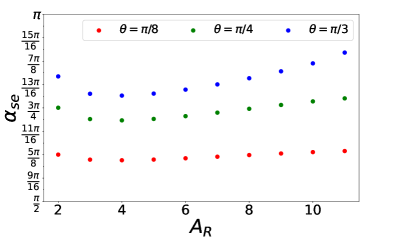
(a) Prolate spheroid

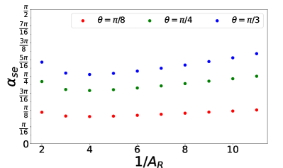
(b) Oblate spheroid

Figure 18: Stable orientation angles $\alpha_{se}$ for prolate and oblate spheroids when the viscosity gradient $\bm{\nabla}\eta$ and the external force $\bm{F}$ are inclined at an angle $\theta$ to each other.

If a steady orientation angle exists, it will be in the plane spanned by $\bm{F}$ and $\bm{\nabla}\eta$ as discussed previously – i.e., $\phi=0$. We set $\phi=0$ and determine the conditions under which $\frac{d\alpha}{dt}=0$ in Eq. (42a). The criterion for a steady orientation angle is:

$$\frac{1}{2}\left(\lambda_{3}+\lambda_{4}\right)\sin(2\alpha)\cos{\theta}-\left(\lambda_{1}-\lambda_{3}\sin^{2}\alpha+\lambda_{4}\cos^{2}{\alpha}\right)\sin{\theta}=0.$$ (43)

For illustration, Fig. 18 plots the steady orientation angles $\alpha_{se}$ for different values of the angle $\theta$ between the external force $\bm{F}$ and $\bm{\nabla}\mathbf{\eta}$. The results are plotted for prolate and oblate spheroids with aspect ratio parameter $A_{R}=5$ and $A_{R}=1/5$, respectively. We observe that $\alpha_{se}$ varies between $\pi/2$ and $\pi$ for prolate spheroids and between $0$ and $\pi/2$ for oblate spheroids. As discussed in the previous sections, these limits are the stable orientations for very high aspect ratio spheroids when the viscosity gradients are parallel and perpendicular to external force. For example, as $\theta\to 0$, we see $\alpha_{se}\rightarrow\pi/2$ for prolate spheroids and $0$ for oblate spheroids, which are the stable orientation for these particles when the viscosity gradient is parallel to the external force.

Lastly, Fig.  19 provides a phase diagram that describes when a steady orientation exists for different particle shapes and viscosity gradient directions. When the viscosity gradient is parallel ($\theta=0$) or anti-parallel ($\theta=\pi$) to the force, there always exists a stable, steady orientation, whereas when the viscosity gradient is perpendicular to the force ($\theta=\pi/2$), there is a range of aspect ratio parameters $A_{R}$ where steady behavior does not exist. At other angles, we observe intermediate behavior between the two limits as illustrated in the figure.

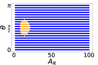
(a) Prolate spheroid

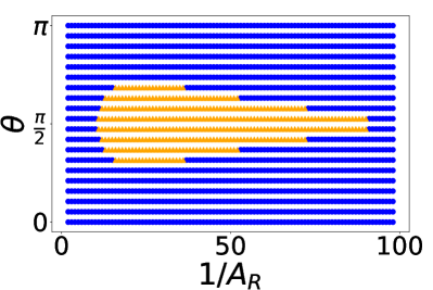
(b) Oblate spheroid

Figure 19: Phase diagram demarcating the region in ($\theta,A_{R}$) space where a stable orientation is reached (blue circles) and where the spheroid tumbles without reaching any stable orientation (yellow triangles). Here ${\theta}$ is the angle between the viscosity gradient $\bm{\nabla\eta}$ and external force $\bm{F}$, while ${A_{R}}$ is the aspect ratio parameter.

5.4 Discussion of applicability of model and incorporating disturbance viscosity

In this paper, we assumed the viscosity field around the particle is a linear function of space and is independent of the flow and the particle geometry. In reality, however, the viscosity field has a more complicated spatial dependence, as it is linked to a scalar field like temperature or concentration that depends on the aforementioned quantities. In this section, we make suggestions on how to incorporate these effects into the analysis and what changes can be expected to the main results.

For illustrative purposes, let us consider a particle in a fluid subject to a temperature gradient $\nabla T$ far away from the particle. The fluid’s viscosity depends linearly on temperature – i.e., $\eta-\eta_{0}=\frac{d\eta}{dT}(T-T_{0})$, and thus the viscosity field also varies spatially around the particle. If the thermal Peclet number is small and the temperature profile is steady, the temperature field will satisfy Laplace’s equation inside and outside the particle: (see (Dassios, 2012) for details):

$$\nabla^{2}T^{out}=0;\qquad\qquad\nabla^{2}T^{in}=0;$$ (44)

This equation is subject to the following boundary conditions: (a) $T^{out}\rightarrow T_{0}+\nabla T\cdot\bm{x}$ far away from the particle ($|\bm{x}|\rightarrow\infty)$, and (b) on the particle surface, the temperatures and fluxes are continuous – i.e., $T^{in}=T^{out}$ and $\left(\bm{n}\cdot\nabla T^{out}\right)=k_{r}\left(\bm{n}\cdot\nabla T^{in}\right)$, where $k_{r}$ is the conductivity ratio between the particle and fluid phase. Once one solves the temperature profile, one can obtain the viscosity field $\eta(\bm{x})$ and then solve for the particle motion in this field. The rigid body motion will still follow the same procedure discussed earlier in the paper – i.e., one performs a perturbation expansion for the viscosity and finds the correction to the rigid body motion via the reciprocal theorem using an extra stress tensor $\tau_{ij}^{ex}=(\eta(\bm{x})-\eta_{0})\gamma_{ij}^{(0)}$. The mobility tensors described in Sec. 4 will take the same form, except the numerical values for the force/rotation mobility coefficients $(\lambda_{1},\lambda_{3},\lambda_{4})$ will be different. For the special cases when one neglects the presence of the particle in the transport equation, or if the conductivity ratio is $k_{r}=1$, the viscosity field will be linear everywhere, and we will recover the results described earlier in the manuscript. Otherwise, the viscosity field will have a more complicated spatial dependence, but the qualitative trends will likely remain the same for the steady orientations and the shape of the particle trajectories. We currently do not have any quantitative results for such an analysis (perhaps to be taken up later in a different paper). But as shown in (Shaik & Elfring, 2021) for swimming spheres, we expect that the disturbance temperature field will only bolster the effects of spatial variation in viscosity, and may not lead to any novel effects. In Appendix E, we outline how one solves Laplace’s equation around an ellipsoidal particle.

6 Conclusion

In this paper, we study a spheroid sedimenting in Newtonian fluid with a viscosity field that varies linearly in space. We employ the principles of linearity, reversibility, symmetry to delineate the mobility relationships for this problem. In the limit of small viscosity gradients, we find that the force/velocity and torque/rotation couplings remain unchanged from the Stokes flow limit. However, the viscosity gradient gives rise to an additional force/rotation and torque/velocity coupling, which is characterized by a third order tensor $M_{ijk}$. The reduced analytical form of this tensor is given by Eq. (29), up to three undetermined coefficients. The values of these coefficients are determined numerically, under the aegis of a reciprocal theorem-based simulation, for a wide range of particle aspect ratios.

Illustrative examples and specific results of our theory are discussed next. Unlike in Stokes flow where the particle orientation stays at its initial orientation during sedimentation, we find that viscosity gradients alter the orientation over time. When the viscosity gradient is along the external force direction, both prolate and oblate spheroids reach a stable orientation where the longest axis is perpendicular to the viscosity gradient. When the viscosity gradient is opposite the external force, the spheroids reach a stable orientation where the longest axis is along to the viscosity gradient. We also show that for most initial orientation angles, the spheroid aquires a drift in a direction transverse to its (main) sedimentation direction until its orientation stabilizes, at which point it moves downward.

When the viscosity gradient and the external force are perpendicular, the plane defined by the viscosity gradient and force is a plane of stability, and the spheroid, irrespective of its initial orientation, will eventually become co-planar with the force and the viscosity gradient. Depending on the particle aspect ratio, the spheroid may continue to rotate in this plane or reach a steady orientation. For the limiting case of a needle-like particle, the prolate spheroid will orient its projector in the direction of the force, while conversely, for the limiting case of a flat disk, the oblate spheroid will orient its projector in the direction of the viscosity gradient. Finally, we note in the general case when the viscosity gradient and external force are neither parallel or perpendicular to each other, the dynamics of the particle is a linear combination of the cases discussed above.

Throughout the analysis, we have neglected the coupling between the viscosity field and the flow or particle motion. Guidelines for incorporating this coupling are presented, using ellipsoidal harmonics to solve the Laplace equation in low $Pe$ limit. However, based on previous literature (Shaik & Elfring, 2021) we believe that such an analysis may not yield any novel results not yet accounted for.

Finally, we remark that even though we employed a perturbative approach to the solution in the limit of weak viscosity gradients, we expect that the steady state behavior – namely the stable orientation of the spheroids – will remain unchanged even when the viscosity gradients become stronger. Stronger viscosity gradients will change the rate at which the stable orientation is attained, but not the value of the steady orientation per se. Lastly, a spheroid is a typical axisymmetric particle with no isotropy but fore-aft symmetry. We believe the qualitative results here will hold for other orientable particles with fore-aft symmetry, and thus can be a model representation of several systems in nature and in industry. Additionally, the current problem may be a stepping stone towards the analysis of more complex systems, for instance flows with linear and quadratic components, or with density (in addition to viscosity) stratification, among others.

Declaration of Interests

The authors report no conflict of interest.

7 Appendix

7.1 Appendix A – Disturbance velocity for an ellipsoid in Stokes flow

Consider a reference frame at an ellpsoid’s center of mass with axes aligned along the particle’s principle axes. From (Kim & Karilla, 2005, pg. 55), the Stokes velocity field around the ellipsoid from external force and torque is the following:

$$v_{i}=\frac{1}{16\pi\eta_{0}}\sum_{j=1}^{3}F_{j}\left[\delta_{ij}G_{0}-x_{j}\frac{\partial G_{0}}{\partial x_{i}}+\frac{a_{j}^{2}}{2}\frac{\partial^{2}G_{1}}{\partial x_{i}\partial x_{j}}\right]$$ (45a)

$$v_{i}=\frac{3}{64\pi\eta_{0}}\sum_{j=1}^{3}\left(\bm{T\times\nabla}\right)_{j}\left[\delta_{ij}G_{1}-x_{j}\frac{\partial G_{1}}{\partial x_{i}}+\frac{a_{j}^{2}}{4}\frac{\partial^{2}G_{2}}{\partial x_{i}\partial x_{j}}\right]$$ (45b)

In these formulas, no summation is assumed for repeated indices unless explicitly stated. To obtain formulas for $v_{ki}^{trans}$ and $v_{ki}^{rot}$ in the reciprocal theorem, we substitute into Eq. (45) the force and torque that comes from unit translation and rotation, respectively.

In the above expressions, the expression for $G_{n}$ is:

$$G_{n}(x,y,z)=\int_{\lambda}^{\infty}\left(\frac{x^{2}}{a^{2}+t}+\frac{y^{2}}{b^{2}+t}+\frac{z^{2}}{c^{2}+t}-1\right)^{n}\frac{dt}{\Delta(t)}$$ (46)

with $\Delta(t)=\sqrt{(a^{2}+t)(b^{2}+t)(c^{2}+t)}$ and $\lambda(x,y,z)$ being the positive root of

$$\frac{x^{2}}{a^{2}+t}+\frac{y^{2}}{b^{2}+t}+\frac{z^{2}}{c^{2}+t}=1$$ (47)

7.2 Appendix B – Resistance formulae for an ellipsoid in Stokes flow

Let us consider a reference frame with the origin at the center of mass of an ellipsoid and the Cartesian axes aligned along the principle axes.

We denote the ellipsoid’s semi-axes as ($a_{1},a_{2},a_{3}$) = ($a,b,c$). In dimensional form, the resistance tensors $R^{FU}$ and $R^{T\omega}$ are diagonal, while the cross-coupling term $R^{F\omega}=R^{TU}=0$. The diagonal elements are:

$$R_{11}^{FU}=\frac{12\eta_{0}V}{\chi_{0}+\alpha_{1}a_{1}^{2}};\quad R_{11}^{T\omega}=\frac{4\eta_{0}V\left(a_{2}^{2}+a_{3}^{2}\right)}{\alpha_{2}a_{2}^{2}+\alpha_{3}a_{3}^{2}}$$ (48)

where $V=\frac{4\pi}{3}a_{1}a_{2}a_{3}$ is the particle volume, and $\left(\chi_{0},\alpha_{1},\alpha_{2}\alpha_{3}\right)$ are elliptic integrals defined below:

$$\begin{gathered}\chi_{0}=\frac{3}{4\pi}V\int_{0}^{\infty}\frac{dt}{\Delta(t)}\\ \alpha_{i}=\frac{3}{4\pi}V\int_{0}^{\infty}\frac{dt}{\left(\mathrm{a}_{\mathrm{i}}^{2}+\mathrm{t}\right)\Delta(t)}\\ \Delta(t)=\sqrt{\left(a_{1}^{2}+t\right)\left(a_{2}^{2}+t\right)\left(a_{3}^{2}+t\right)}\end{gathered}$$

The other elements of the diagonal tensors are obtained by index cycling.

The mobility matrix is the inverse of the resistance matrix, and hence given by the inverse of the diagonal elements above. For the special case when the particle is a spheroid with $a_{1}\neq a_{2}=a_{3}$, the coefficients $c_{1}-c_{4}$ for the mobility matrix in Eq. (25a) and Eq. (25b) are:

$$c_{1}=\frac{1}{R_{22}^{FU}};\quad c_{2}=\frac{1}{R_{11}^{FU}};\quad c_{3}=\frac{1}{R_{22}^{T\omega}};\quad c_{4}=\frac{1}{R_{11}^{T\omega}}$$

These coefficients have analytical formulae (see pgs 64 and 68 in Kim and Karilla). Using the notation in this paper, we obtain for prolate and oblate spheroids:

• Prolate spheroids

  $$c_{1} =\frac{1}{6\pi\eta_{0}a}\frac{1}{Y_{A}}; Y_{A}=\frac{16}{3}e^{3}\left[2e+(3e^{2}-1)L\right]^{-1}$$ (49a)

  $$c_{2} =\frac{1}{6\pi\eta_{0}a}\frac{1}{X_{A}} X_{A}=\frac{8}{3}e^{3}\left[-2e+(1+e^{2})L\right]^{-1}$$ (49b)

  $$c_{3} =\frac{1}{8\pi\eta_{0}a^{3}}\frac{1}{Y_{C}} Y_{C}=\frac{4}{3}e^{3}(2-e^{2})\left[-2e+(1+e^{2})L\right]^{-1}$$ (49c)

  $$c_{4} =\frac{1}{8\pi\eta_{0}a^{3}}\frac{1}{X_{C}} X_{C}=\frac{4}{3}e^{3}(1-e^{2})\left[2e-(1-e^{2})L\right]^{-1}$$ (49d)

  where $e=\sqrt{1-\frac{b^{2}}{a^{2}}}$ is the spheroid’s eccentricity and $L=\ln\left(\frac{1+e}{1-e}\right)$. To get the non-dimensional form used in the manuscript, we multiply $c_{1}$ and $c_{2}$ by $6\pi\eta_{0}R=6\pi\eta_{0}(ab^{2})^{1/3}$, and multiply $c_{3}$ and $c_{4}$ by $6\pi\eta_{0}R^{3}=6\pi\eta_{0}ab^{2}$.
  

• Oblate spheroids

  $$c_{1} =\frac{1}{6\pi\eta_{0}b}\frac{1}{Y_{A}}; Y_{A}=\frac{8}{3}e^{3}\left[(2e^{2}+1)C-e\sqrt{1-e^{2}}\right]^{-1}$$ (50a)

  $$c_{2} =\frac{1}{6\pi\eta_{0}b}\frac{1}{X_{A}} X_{A}=\frac{4}{3}e^{3}\left[(2e^{2}-1)C+e\sqrt{1-e^{2}}\right]^{-1}$$ (50b)

  $$c_{3} =\frac{1}{8\pi\eta_{0}b^{3}}\frac{1}{Y_{C}} Y_{C}=\frac{2}{3}e^{3}(2-e^{2})\left[e\sqrt{1-e^{2}}-(1-2e^{2})C\right]^{-1}$$ (50c)

  $$c_{4} =\frac{1}{8\pi\eta_{0}b^{3}}\frac{1}{X_{C}} X_{C}=\frac{2}{3}e^{3}\left[C-e\sqrt{1-e^{2}}\right]^{-1}$$ (50d)

  where $e=\sqrt{1-\frac{a^{2}}{b^{2}}}$ is the spheroid’s eccentricity and $C=\cot^{-1}\left(\frac{\sqrt{1-e^{2}}}{e}\right)$. To get the non-dimensional form used in the manuscript, we multiply $c_{1}$ and $c_{2}$ by $6\pi\eta_{0}R=6\pi\eta_{0}(ab^{2})^{1/3}$, and multiply $c_{3}$ and $c_{4}$ by $6\pi\eta_{0}R^{3}=6\pi\eta_{0}ab^{2}$.

7.3 Appendix C – Reciprocal theorem and $O(\beta)$ solution

To delineate the $\mathcal{O}(\beta)$ correction to the particle kinematics – i.e., obtain the solution for ($U_{i}^{(1)},\omega_{i}^{(1)}$) – there are two approaches possible. The brute force approach is to solve the velocity and stress field around the particle, and then integrate the stress on the particle’s surface to find the polymeric force and torque. However, this approach is tedious and analytically intractable for complicated geometries. Instead, we circumvent the calculation of the velocity and the stress field around the particle and directly obtain the polymeric force and torque using the reciprocal theorem (Leal, 1980).

First, we note that the fluid stress field at $\mathcal{O}(\beta)$ has two parts:

$$\sigma_{ij}^{(1)}=\dot{\gamma}_{ij}^{(1)}-p^{(1)}\delta_{ij}+\tau_{ij}^{ex}.$$ (51)

One is the Newtonian part given by $\dot{\gamma}_{ij}^{(1)}-p^{(1)}\delta_{ij}$. The other part is polymeric, denoted as $\tau_{ij}^{\text{ex}}$ and given by:

$$\tau_{ij}^{ex}=(\hat{d}_{k}x_{k})\dot{\gamma}_{ij}^{(0)}$$ (52)

We note the important observation that the polymeric stress at $\mathcal{O}(\beta)$ depends on the strain rate at leading order.

In the spirit of the reciprocal theorem, we define an auxiliary problem wherein the same particle, at the same location and same orientation, is sedimenting in a Newtonian fluid with a constant (spatially invariant) viscosity. The quantities pertaining to the auxiliary problem are denoted by the aux superscript. Therefore, the external force and the torque acting on the particle in the auxiliary problem is given by $F_{i}^{aux},T_{i}^{aux}$ and its rigid body motion is given by $U_{i}^{aux},\omega^{aux}_{i}$. The flow field around the particle is $v_{i}^{aux}$, while the stress field is $\sigma_{ij}^{aux}$, expressed as:

$$\sigma_{ij}^{aux}=\dot{\gamma}_{ij}^{aux}-p^{aux}\delta_{ij}$$ (53)

Since the stress field of the auxiliary problem and that of the $\mathcal{O}(\beta)$ problem are divergence free:

$$\frac{\partial\sigma_{ij}^{aux}}{\partial x_{j}}=\frac{\partial\sigma_{ij}^{(1)}}{\partial x_{j}}=0,$$ (54)

or,

$$v_{i}^{(1)}\frac{\partial\sigma_{ij}^{aux}}{\partial x_{j}}=v_{i}^{aux}\frac{\partial\sigma_{ij}^{(1)}}{\partial x_{j}}=0,$$ (55)

Using the product rule, the above equation reduces to:

$$\frac{\partial v_{i}^{(1)}\sigma_{ij}^{aux}}{\partial x_{j}}-\frac{\partial v_{i}^{aux}\sigma_{ij}^{(1)}}{\partial x_{j}}=\sigma_{ij}^{aux}\frac{\partial v_{i}^{(1)}}{\partial x_{j}}-\sigma_{ij}^{(1)}\frac{\partial v_{i}^{aux}}{\partial x_{j}}$$ (56)

We now substitute the expressions $\sigma_{ij}^{aux}=\dot{\gamma}_{ij}^{aux}-p^{aux}\delta_{ij}$ and $\sigma_{ij}^{(1)}=\dot{\gamma}_{ij}^{(1)}-p^{(1)}\delta_{ij}+\tau_{ij}^{ex,(0)}$ to the right hand side. Using the identities $\frac{\partial v_{i}}{\partial x_{i}}=\frac{\partial v_{i}^{aux}}{\partial x_{i}}=0$ and $\dot{\gamma}_{ij}^{(1)}\frac{\partial v_{i}^{aux}}{\partial x_{j}}=\dot{\gamma}_{ij}^{aux}\frac{\partial v_{i}^{(1)}}{\partial x_{j}}$, we obtain:

$$\frac{\partial v_{i}^{(1)}\sigma_{ij}^{aux}}{\partial x_{j}}-\frac{\partial v_{i}^{aux}\sigma_{ij}^{(1)}}{\partial x_{j}}=-\tau_{ij}^{ex,(0)}\frac{\partial v_{i}^{aux}}{\partial x_{j}},$$ (57)

Next, we integrate the above equation over the volume outside the particle and use the divergence theorem. This procedure yields:

$$\int_{\mathcal{S}}n_{j}v_{i}^{(1)}\sigma_{ij}^{aux}dS=\int_{\mathcal{S}}n_{j}v_{i}^{aux}\sigma_{ij}^{(1)}dS+\int_{V}\tau_{ij}^{ex,(0)}\frac{\partial v_{i}^{aux}}{\partial x_{j}}dV,$$ (58)

where $\mathcal{S}$ is the surface of the particle and $n_{j}$ is the normal to the particle surface pointing inside the fluid. On particle surface, $v_{i}^{(1)}$ and $v_{i}^{aux}$ are rigid body motion – i.e., $v_{i}^{(1)}=U_{i}^{(1)}+\epsilon_{ijk}\omega_{j}^{(1)}x_{k}$ and $v_{i}^{aux}=U_{i}^{aux}+\epsilon_{ijk}\omega_{j}^{aux}x_{k}$. Substituting these expressions into the surface integrals yield:

$$-F_{i}^{aux}U_{i}^{(1)}-T_{i}^{aux}\omega_{i}^{(1)}=\int_{V}\tau_{ij}^{ex,(0)}\frac{\partial v_{i}^{aux}}{\partial x_{j}}dV$$ (59)

Note when deriving the above expression, we made use of the fact that the force and torque acting on the particle at $O(\beta)$ is zero ($F_{i}^{(1)}=T_{i}^{(1)}=0$). Lastly, let us write the auxillary force and torque as a linear combination of the rigid body velocities using the resistance tensors for the particle:

$$F_{i}^{aux} =R_{ij}^{FU}U_{j}^{aux}+R_{ij}^{F\omega}\omega_{j}^{aux}$$ (60)

$$T_{i}^{aux} =R_{ij}^{TU}U_{j}^{aux}+R_{ij}^{T\omega}\omega_{j}^{aux}$$

where in the above equation, the resistance tensors satisfy the following symmetry relationships: $\bm{R}^{FU}=(\bm{R}^{FU})^{T}$, $\bm{R}^{T\omega}=(\bm{R}^{T\omega})^{T}$, and $\bm{R}^{F\omega}=(\bm{R}^{TU})^{T}$. We will also write the auxillary velocity field in the volume integral for Eq. (59) as a linear combination of the rigid body motions:

$$v_{i}^{aux}=v_{ik}^{trans}U_{k}^{aux}+v_{ik}^{rot}\omega_{k}^{aux}$$ (61)

where $v_{ik}^{rot}$ and $v_{ik}^{rot}$ are the velocity fields in the $i$ direction induced by unit translation or rotation in the $k$ direction. Substituting Eqs. (60) and (61) into (59) and eliminating $U_{i}^{aux}$ and $\omega_{i}^{aux}$ yields the final result (Eq. (16)) stated in the manuscript.

7.4 Appendix D – Simplification of mobility tensor $M_{ijk}$

Here, we show that Eq. (28) is equivalent to Eq. (29). To that end, we re-write Eq. (28) as:

$$M_{ijk}=\lambda_{1}\underbrace{\epsilon_{ijk}}_{\text{Term 1}}+\lambda_{2}\underbrace{p_{i}\epsilon_{jkq}p_{q}}_{\text{Term2}}+\lambda_{3}\underbrace{p_{j}\epsilon_{ikq}p_{q}}_{\text{Term3}}+\lambda_{4}\underbrace{p_{k}\epsilon_{ijq}p_{q}}_{\text{Term4}}$$ (62)

Without any loss of generality, we assume a particular orientation of the projection vector $p_{i}$ namely $p_{i}=\delta_{i1}$ (and so on). Therefore, Eq. (63) may be written as:

$$M_{ijk}=\lambda_{1}\underbrace{\epsilon_{ijk}}_{\text{Term 1}}+\lambda_{2}\underbrace{\delta_{i1}\epsilon_{jk1}}_{\text{Term2}}+\lambda_{3}\underbrace{\delta_{j1}\epsilon_{ik1}}_{\text{Term3}}+\lambda_{4}\underbrace{\delta_{k1}\epsilon_{ij1}}_{\text{Term4}}$$ (63)

Say,

$$M_{ijk}^{(1)} =\text{Term 1}=\epsilon_{ijk}$$ (64a)

$$M_{ijk}^{(2)} =\text{Term 2}=\delta_{i1}\epsilon_{jk1}$$ (64b)

$$M_{ijk}^{(3)} =\text{Term 3}=\delta_{j1}\epsilon_{ik1}$$ (64c)

$$M_{ijk}^{(4)} =\text{Term 4}=\delta_{k1}\epsilon_{ij1}$$ (64d)

To expand the different tensors, term by term, we find that the only nonzero terms in $M_{ijk}^{(1)}$ are:

$$M_{123}^{(1)}=M_{312}^{(1)}=M_{231}^{(1)}=1$$ (65a)

$$M_{132}^{(1)}=M_{321}^{(1)}=M_{213}^{(1)}=-1$$ (65b)

Similarly, the nonzero terms in $M_{ijk}^{(2)}$ are given as:

$$M_{123}^{(2)}=1$$ (66a)

$$M_{132}^{(2)}=-1$$ (66b)

and the nonzero terms in $M_{ijk}^{(3)}$ are given as:

$$M_{213}^{(3)}=-1$$ (67a)

$$M_{312}^{(3)}=1$$ (67b)

whilst, the nonzero terms in $M_{ijk}^{(4)}$ are given as:

$$M_{231}^{(4)}=1$$ (68a)

$$M_{321}^{(4)}=-1$$ (68b)

From the visual inspection of Eqs. (65), (66), (67), (68), we obtain the following relationship:

$$M_{ijk}^{(1)}=M_{ijk}^{(2)}+M_{ijk}^{(3)}+M_{ijk}^{(4)},$$ (69)

which means out of the four terms $M_{ijk}^{(1)}$,$M_{ijk}^{(2)}$,$M_{ijk}^{(3)}$ and $M_{ijk}^{(4)}$, only $3$ are linearly independent, and therefore, without loss of generality, we can remove $M_{ijk}^{(2)}$ ($=\text{Term2}$) from Eq. (63) (or Eq. (28)), which leads to, with slight change in notation, Eq. (29).

7.5 Appendix E – Solving Laplace equation around an ellipsoid with a far field temperature gradient

Here we outline how to solve Laplace’s equation around an ellipsoidal particle. We will use ellipsoidal harmonics, a technique is widely used in electrostatics, and the results in papers (Sten, 2006) directly apply here. Let us consider a frame of reference where the Cartesian coordinate system $(x,y,z)$ aligns with the semi-major axes $(a,b,c)$ of the ellipsoid, with $a\geq b\geq c$. If the far-field temperature is:

$$T^{\infty}(\bm{x})=T_{0}+\frac{\partial T}{\partial x}x+\frac{\partial T}{\partial y}y+\frac{\partial T}{\partial z}z$$ (70)

the solution outside the ellipsoid takes the following form:

$$T(\bm{x})=T^{\infty}(\bm{x})+\sum_{p=1}^{3}B_{1p}\mathcal{F}_{1}^{p}(\bm{x})$$ (71)

In the above equation, $\mathcal{F}_{1}^{p}(\bm{x})=F_{1}^{p}(\xi)E_{1}^{p}(\mu)E_{1}^{p}(\nu)$ are decaying ellipsoidal harmonics using the ellipsoidal coordinate system $(\xi,\mu,\nu)$, where $\xi=a$ denotes the surface of the ellipsoid. The functions $E_{1}^{p}$ and $F_{1}^{p}$ are Lame functions of the first and second kind, defined in publication (Sten, 2006). In Eq. (71), the coefficients $B_{1p}$ are the following:

$$B_{11} =\frac{abc}{3}\frac{1}{kh}\frac{(1–k_{r})}{1+L_{1}^{1}(a)(k_{r}-1)}\frac{\partial T}{\partial x}$$ (72a)

$$B_{12} =\frac{abc}{3}\frac{1}{h\sqrt{k^{2}–h^{2}}}\frac{(1–k_{r})}{1+L_{1}^{2}(a)(k_{r}-1)}\frac{\partial T}{\partial y}$$ (72b)

$$B_{13} =\frac{abc}{3}\frac{1}{k\sqrt{k^{2}–h^{2}}}\frac{(1–k_{r})}{1+L_{1}^{3}(a)(k_{r}-1)}\frac{\partial T}{\partial z}$$ (72c)

where $k=\sqrt{a^{2}–c^{2}}$ and $h=\sqrt{a^{2}–b^{2}}$. The geometric factors $L_{1}^{1,2,3}(a)$ take the following form (Sten, 2006):

$$L_{1}^{1,2,3}(a)=abc\int_{a}^{\infty}\frac{d\xi’}{\left[E_{1}^{1,2,3}(\xi’)\right]^{2}\sqrt{\left(\xi^{\prime 2}–h^{2}\right)\left(\xi^{\prime 2}–k^{2}\right)}}$$ (73)

References

- Anand (2014) Anand, Vishal 2014 Slip law effects on heat transfer and entropy generation of pressure driven flow of a power law fluid in a microchannel under uniform heat flux boundary condition. Energy 76, 716–732.
- Anand (2016) Anand, V. 2016 Effect of slip on heat transfer and entropy generation characteristics of simplified Phan-Thien-Tanner fluids with viscous dissipation under uniform heat flux boundary conditions: Exponential formulation. Applied Thermal Engineering 98.
- Anand & Christov (2019a) Anand, V. & Christov, I. C. 2019a On the Deformation of a Hyperelastic Tube Due to Steady Viscous Flow Within. In Dynamical Processes in Generalized Continua and Structures (ed. H. Altenbach, A. Belyaev, V. A. Eremeyev, A. Krivtsov & A. V. Porubov), Springer Series on Advanced Structured Materials, vol. 103, chap. 2, pp. 17–35. Cham, Switzerland: Springer Nature.
- Anand & Christov (2019b) Anand, Vishal & Christov, Ivan C. 2019b On the enhancement of heat transfer and reduction of entropy generation by asymmetric slip in pressure-driven non-Newtonian microflows. Journal of Heat Transfer 141 (2).
- Anand & Christov (2020) Anand, V. & Christov, I. C. 2020 Transient compressible flow in a compliant viscoelastic tube. Phys. Fluids 32, 112014.
- Anand & Christov (2021) Anand, V. & Christov, I. C. 2021 Revisiting steady viscous flow of a generalized Newtonian fluid through a slender elastic tube using shell theory. Z. Angew. Math. Mech. (ZAMM) 101, e201900309.
- Anand & Narsimhan (2023) Anand, Vishal & Narsimhan, Vivek 2023 Dynamics of spheroids in pressure driven flows of shear thinning fluids .
- Anand et al. (2019) Anand, V., Rathinaraj, J. D. J. & Christov, I. C. 2019 Non-Newtonian fluid–structure interactions: Static response of a microchannel due to internal flow of a power-law fluid. J. Non-Newtonian Fluid Mech. 264, 62–72.
- Ardekani et al. (2017) Ardekani, Arezoo M., Doostmohammadi, Amin & Desai, Nikhil 2017 Transport of particles, drops, and small organisms in density stratified fluids. Physical Review Fluids 2 (10), 100503.
- Arrigo et al. (1999) Arrigo, Kevin R, Robinson, Dale H, Worthen, Denise L, Dunbar, Robert B, DiTullio, Giacomo R, VanWoert, Michael & Lizotte, Michael P 1999 Phytoplankton Community Structure and the Drawdown of Nutrients and CO¡sub¿2¡/sub¿ in the Southern Ocean. Science 283 (5400), 365–367.
- Asghar et al. (2020) Asghar, Zeeshan, Javid, Khurram, Waqas, Muhammad, Ghaffari, Abuzar & Khan, Waqar Azeem 2020 Cilia-driven fluid flow in a curved channel: effects of complex wave and porous medium. Fluid Dynamics Research 52 (1), 015514.
- Auguste et al. (2013) Auguste, Franck, Magnaudet, Jacques & Fabre, David 2013 Falling styles of disks. Journal of Fluid Mechanics 719, 388–405.
- Butler & Shaqfeh (2002) Butler, Jason E. & Shaqfeh, Eric S.G. 2002 Dynamic simulations of the inhomogeneous sedimentation of rigid fibres. Journal of Fluid Mechanics 468, 205–237.
- Cox (1965) Cox, R. G. 1965 The steady motion of a particle of arbitrary shape at small Reynolds numbers. Journal of Fluid Mechanics 23 (4), 625–643.
- Dabade et al. (2015) Dabade, Vivekanand, Marath, Navaneeth K. & Subramanian, Ganesh 2015 Effects of inertia and viscoelasticity on sedimenting anisotropic particles. Journal of Fluid Mechanics 778, 133–188.
- Dandekar & Ardekani (2020) Dandekar, Rajat & Ardekani, Arezoo M. 2020 Swimming sheet in a viscosity-stratified fluid. Journal of Fluid Mechanics .
- Dandekar et al. (2020) Dandekar, Rajat, Shaik, Vaseem A. & Ardekani, Arezoo M. 2020 Motion of an arbitrarily shaped particle in a density stratified fluid. Journal of Fluid Mechanics 890, A16.
- Dassios (2012) Dassios, George 2012 Ellipsoidal Harmonics: Theory and Applications. Ellipsoidal Harmonics .
- Datt & Elfring (2019) Datt, Charu & Elfring, Gwynn J. 2019 Active Particles in Viscosity Gradients. Physical Review Letters 123 (15).
- Doostmohammadi et al. (2014) Doostmohammadi, A., Dabiri, S. & Ardekani, A. M. 2014 A numerical study of the dynamics of a particle settling at moderate Reynolds numbers in a linearly stratified fluid. Journal of Fluid Mechanics 750, 5–32.
- Du et al. (2012) Du, Jian, Keener, James P., Guy, Robert D. & Fogelson, Aaron L. 2012 Low-Reynolds-number swimming in viscous two-phase fluids. Physical Review E 85 (3), 036304.
- Eastham & Shoele (2020) Eastham, Patrick S. & Shoele, Kourosh 2020 Axisymmetric squirmers in Stokes fluid with nonuniform viscosity. Physical Review Fluids 5 (6).
- Esparza López et al. (2021) Esparza López, Christian, Gonzalez-Gutierrez, Jorge, Solorio-Ordaz, Francisco, Lauga, Eric & Zenit, Roberto 2021 Dynamics of a helical swimmer crossing viscosity gradients. Physical Review Fluids 6 (8).
- Gagnon & Arratia (2016) Gagnon, D. A. & Arratia, P. E. 2016 The cost of swimming in generalized Newtonian fluids: experiments with C. elegans. Journal of Fluid Mechanics 800, 753–765.
- Galdi (2000) Galdi, Giovanni P. 2000 Slow steady fall of rigid bodies in a second-order fluid. Journal of Non-Newtonian Fluid Mechanics 90 (1), 81–89.
- Galdi et al. (2011) Galdi, Giovanni P., Vaidya, Ashwin, Pokorný, Milan, Joseph, Daniel D. & Feng, Jimmy 2011 Orientation of symmetric bodies falling in a second-order liquid at nonzero Reynolds number. Mathematical Models and Methods in Applied Sciences 12 (11), 1653–1690.
- Hanazaki et al. (2009) Hanazaki, H., Konishi, K. & Okamura, T. 2009 Schmidt-number effects on the flow past a sphere moving vertically in a stratified diffusive fluid. Physics of Fluids 21 (2), 026602.
- Hatwalne et al. (2004) Hatwalne, Yashodhan, Ramaswamy, Sriram, Rao, Madan & Simha, R. Aditi 2004 Rheology of Active-Particle Suspensions. Physical Review Letters 92 (11), 118101.
- Herzhaft & Guazzelli (1999) Herzhaft, Benjamin & Guazzelli, Elisabeth 1999 Experimental study of the sedimentation of dilute and semi-dilute suspensions of fibres. Journal of Fluid Mechanics 384, 133–158.
- Howard Berg (2004) Howard Berg 2004 E. coli in Motion, 1st edn. New York, NY: Springer New York.
- Jacquemin et al. (2006) Jacquemin, J., Husson, P., Padua, A. A.H. & Majer, V. 2006 Density and viscosity of several pure and water-saturated ionic liquids. Green Chemistry 8 (2), 172–180.
- Khayat & Cox (1989) Khayat, R. E. & Cox, R. G. 1989 Inertia effects on the motion of long slender bodies. Journal of Fluid Mechanics 209, 435–462.
- Kim (1986) Kim, Sangtae 1986 THE MOTION OF ELLIPSOIDS IN A SECOND ORDER FLUID. Journal of Non-Newtonian Fluid Mechanics 21, 255–269.
- Kim & Karilla (2005) Kim, Sangtae & Karilla, Seppo 2005 Microhydrodynamics: Principles and Selected Application, 2nd edn. Mineola, New York: Dover Publications.
- Kim et al. (2016) Kim, Sangwon, Lee, Seungmin, Lee, Jeonghun, Nelson, Bradley J., Zhang, Li & Choi, Hongsoo 2016 Fabrication and manipulation of ciliary microrobots with non-reciprocal magnetic actuation. Scientific Reports 6.
- Koch & Shaqfeh (1989) Koch, Donald L. & Shaqfeh, Eric S. G. 1989 The instability of a dispersion of sedimenting spheroids. Journal of Fluid Mechanics 209, 521–542.
- Koch & Shaqfeh (1991) Koch, Donald L. & Shaqfeh, E. S. G. 1991 Screening in sedimenting suspensions. Journal of Fluid Mechanics 224, 275–303.
- Kuusela et al. (2003) Kuusela, E., Lahtinen, J. M. & Ala-Nissila, T. 2003 Collective Effects in Settling of Spheroids under Steady-State Sedimentation. Physical Review Letters 90 (9), 4.
- Leal (1980) Leal, L G 1980 Particle motions in a viscous fluid. Ann. Rev. Fluid Mech 12, 435–76.
- Leal (2007) Leal, L Gary 2007 Advanced transport phenomena: fluid mechanics and convective transport processes, , vol. 7. Cambridge University Press.
- Li et al. (2017) Li, Jinxing, Ávila, Berta Esteban Fernández De, Gao, Wei, Zhang, Liangfang & Wang, Joseph 2017 Micro/nanorobots for biomedicine: Delivery, surgery, sensing, and detoxification. Science Robotics 2 (4).
- Liebchen et al. (2018) Liebchen, Benno, Monderkamp, Paul, ten Hagen, Borge & Löwen, Hartmut 2018 Viscotaxis: Microswimmer Navigation in Viscosity Gradients. Physical Review Letters 120 (20), 208002.
- Lofquist & Purtell (1984) Lofquist, Karl E. B. & Purtell, L. Patrick 1984 Drag on a sphere moving horizontally through a stratified liquid. Journal of Fluid Mechanics 148, 271–284.
- Mehaddi et al. (2018) Mehaddi, R., Candelier, F. & Mehlig, B. 2018 Inertial drag on a sphere settling in a stratified fluid. Journal of Fluid Mechanics 855, 1074–1087.
- More & Ardekani (2022) More, Rishabh V & Ardekani, Arezoo M 2022 Annual Review of Fluid Mechanics Motion in Stratified Fluids. Annu. Rev. Fluid Mech. 2023 55, 157–192.
- More et al. (2021) More, Rishabh V., Ardekani, Mehdi N., Brandt, Luca & Ardekani, Arezoo M. 2021 Orientation instability of settling spheroids in a linearly density-stratified fluid. Journal of Fluid Mechanics 929.
- Nelson et al. (2010) Nelson, Bradley J., Kaliakatsos, Ioannis K. & Abbott, Jake J. 2010 Microrobots for minimally invasive medicine.
- Nicolai et al. (1998) Nicolai, H., Herzhaft, B., Hinch, E. J., Oger, L. & Guazzelli, E. 1998 Particle velocity fluctuations and hydrodynamic self‐diffusion of sedimenting non‐Brownian spheres. Physics of Fluids 7 (1), 12.
- Palagi et al. (2013) Palagi, Stefano, Jager, Edwin WH, Mazzolai, Barbara & Beccai, Lucia 2013 Propulsion of swimming microrobots inspired by metachronal waves in ciliates: from biology to material specifications. Bioinspiration & Biomimetics 8 (4), 046004.
- Qin & Pak (2023) Qin, Ke & Pak, On Shun 2023 Purcell’s swimmer in a shear-thinning fluid. Phys. Rev. Fluids 8 (3), 33301.
- Rafaï et al. (2010) Rafaï, Salima, Jibuti, Levan & Peyla, Philippe 2010 Effective Viscosity of Microswimmer Suspensions. Physical Review Letters 104 (9), 098102.
- Shaik & Elfring (2021) Shaik, Vaseem A. & Elfring, Gwynn J. 2021 On the hydrodynamics of active particles in viscosity gradients. Physical Review of Fluids .
- Shin et al. (2006) Shin, Mansoo, Koch, Donald L. & Subramanian, Ganesh 2006 A pseudospectral method to evaluate the fluid velocity produced by an array of translating slender fibers. Physics of Fluids 18 (6), 063301.
- Shin et al. (2009) Shin, Mansoo, Koch, Donald L. & Subramanian, Ganesh 2009 Structure and dynamics of dilute suspensions of finite-Reynolds-number settling fibers. Physics of Fluids 21 (12), 123304.
- Sokolov & Aranson (2009) Sokolov, Andrey & Aranson, Igor S. 2009 Reduction of Viscosity in Suspension of Swimming Bacteria. Physical Review Letters 103 (14), 148101.
- Sten (2006) Sten, Johan C.-E. 2006 Ellipsoidal harmonics and their application in electrostatics. Journal of Electrostatics 64 (10), 647–654.
- Takabe et al. (2017) Takabe, Kyosuke, Tahara, Hajime, Islam, Md Shafiqul, Affroze, Samia, Kudo, Seishi & Nakamura, Shuichi 2017 Viscosity-dependent variations in the cell shape and swimming manner of Leptospira. Microbiology (United Kingdom) 163 (2), 153–160.
- Varanasi & Subramanian (2022) Varanasi, Arun Kumar & Subramanian, Ganesh 2022 Motion of a sphere in a viscous density stratified fluid. Journal of Fluid Mechanics 949, A29.
- Venkatesh et al. (2022) Venkatesh, Anirudh, Anand, Vishal & Narsimhan, Vivek 2022 Peeling of linearly elastic sheets using complex fluids at low Reynolds numbers. Journal of non Newtonian fluid mechanics .
- Vishnampet & Saintillan (2012) Vishnampet, Ramanathan & Saintillan, David 2012 Concentration instability of sedimenting spheres in a second-order fluid. Physics of Fluids 24 (7), 073302.
- Wang et al. (2020) Wang, Shiyan, Tai, Cheng Wei & Narsimhan, Vivek 2020 Dynamics of spheroids in an unbound quadratic flow of a general second-order fluid. Physics of Fluids 32 (11).
- YICK et al. (2009) YICK, KING YEUNG, TORRES, CARLOS R., PEACOCK, THOMAS & STOCKER, ROMAN 2009 Enhanced drag of a sphere settling in a stratified fluid at small Reynolds numbers. Journal of Fluid Mechanics 632, 49–68.
- Zhuang et al. (2017) Zhuang, Jiang, Park, Byung Wook & Sitti, Metin 2017 Propulsion and Chemotaxis in Bacteria-Driven Microswimmers. Advanced Science 4 (9).