Sparsity-Aware Optimal Transport for Unsupervised Restoration Learning

Abstract

Recent studies show that, without any prior model, the unsupervised restoration learning problem can be optimally formulated as an optimal transport (OT) problem, which has shown promising performance on denoising tasks to approach the performance of supervised methods. However, it still significantly lags behind state-of-the-art supervised methods on complex restoration tasks such as super-resolution, deraining, and dehazing. In this paper, we exploit the sparsity of degradation in the OT framework to significantly boost its performance on these tasks. First, we disclose an observation that the degradation in these tasks is quite sparse in the frequency domain, and then propose a sparsity-aware optimal transport (SOT) criterion for unsupervised restoration learning. Further, we provide an analytic example to illustrate that exploiting the sparsity helps to reduce the ambiguity in finding an inverse map for restoration. Experiments on real-world super-resolution, deraining, and dehazing demonstrate that SOT can improve the PSNR of OT by about 2.6 dB, 2.7 dB and 1.3 dB, respectively, while achieving the best perception scores among the compared supervised and unsupervised methods. Particularly, on the three tasks, SOT significantly outperforms existing unsupervised methods and approaches the performance of state-of-the-art supervised methods.

1 Introduction

Image restoration plays a fundamental role in low-level computer vision, which has attracted much research attention in the past few decades. Traditional model based methods typically utilize prior models of image and/or degradation, such as sparsity, low-rankness, smoothness, self-similarity or other priors of natural image, and Gaussianity, spatially independent i.i.d. of noise [1, 2, 3, 4, 5]. Recently, benefited from the powerful deep learning techniques, the field of image restoration has made much progress in the past few years [6, 7].

Generally, the success of deep network based methods usually rely on sufficient paired degraded-clean data. Nevertheless, in some applications such paired data is difficult or even impractical to collect. For such applications, as a common practice, synthesized degraded-clean data can be used to learn a restoration model. However, the gap between synthesized and real-world data limits the practical performance of the learned model on real-world data, especially when the degradation is too complex to accurately simulate. In these circumstances, unsupervised methods without requiring any degraded-clean pairs are preferred.

To relax the requirement of paired training data, unsupervised learning methods have recently been actively studied for various image restoration tasks. For example, for unsupervised/self-supervised denoising learning, the noise-to-noise (N2N) [8], noise-to-void (N2V) [9], noise-to-self (N2S) [10] methods, as well as many variants have been developed, see [11, 12, 13, 14, 15] and the references therein. While N2N uses noisy pairs, N2V and N2S learn the restoration models in a self-supervised manner. Typically, these methods rely on prior assumptions, such as the noise in noisy pairs are independent [8, 11, 13], or the noise is spatially independent and/or the noise type is a priori known [9, 10, 14, 15]. Such assumptions limit the performance when the noise does not well conform with the assumptions.

In the recent work [16], it has been shown that, in the absence of any prior model of the degradation, the unsupervised restoration learning problem can be optimally formulated as an optimal transport (OT) problem. The OT criterion based unsupervised learning method has achieved promising performance on various denoising tasks to approach the performance of supervised methods. However, it still significantly lags behind state-of-the-art supervised methods on more complex restoration tasks such as super-resolution, deraining, and dehazing. A main reason is that, for these restoration tasks, seeking an inverse of the degradation map is more ambiguous. In light of this understanding, this work is motivated to exploit prior models of the degradation in the OT criterion to reduce the ambiguity in learning an inverse map of the degradation.

Specifically, in this work, we exploit the sparsity of degradation in the OT framework to significantly boost the performance on these complex restoration tasks. The main contributions are as follows.

First, we disclose an empirical observation that, for the super-resolution, deraining, and dehazing tasks, the degradation is quite sparse in the frequency domain. Based on this observation, we propose a sparsity-aware optimal transport (SOT) criterion for unsupervised restoration learning.

Then, we provide an analysis to illustrate that exploiting the sparsity of degradation in the OT criterion helps to reduce the ambiguity in finding an inverse map of the degradation.

Finally, we provide extensive experimental results on both synthetic and real-world data for the super-resolution, deraining, and dehazing tasks. The results demonstrate that exploiting the sparsity of degradation can significantly boost the performance of the OT criterion. For example, compared with the vanilla OT criterion on real-world super-resolution, deraining and dehazing, it achieves a PSNR improvement of about 2.6 dB, 2.7 dB and 1.3 dB, respectively, and at meantime, attains the best perception scores among the compared supervised and unsupervised methods. Meanwhile, in synthetic data experiments on the three tasks, the PSNR improvement is about 2.5, 1.6, 3.4 dB, respectively. Noteworthily, on all the tasks, SOT considerably outperforms existing unsupervised methods to approach the performance of state-of-the-art supervised methods.

Our work provides a generic unsupervised (unpaired) learning framework, which applies to various restoration applications as long as the degradation can be sparsely represented. Relaxing the requirement of collecting or synthesizing paired degraded-clean data is of practical importance, especially for applications where paired data is difficult to collect or accurately simulate. In such realistic circumstances, the proposed method has much potential as it shows favorable performance on real-world data even compared with state-of-the-art supervised methods.

2 Related Work

We review the works related to this work, especially on unsupervised methods in various image restoration tasks.

Image denoising. Traditional hand-crafted model based denoising methods typically design models based on a priori information on the signal and noise [17, 1, 2, 18]. The performance of these methods is usually closely related to hyperparameter setting. Recently, deep learning methods without requiring paired noisy-clean data have attracted active attention. The N2N method [8], as well as its variants [11, 19, 20, 21], utilize noisy pairs to train restoration models under the assumption that the noise is zero-mean and independent homogeneous across paired samples. Self-supervised methods adopt special networks or training methods that extract information from the noisy image itself for supervised learning, e.g. adopting a blind-spot network to predict masked pixel by neighboring pixels or designing sampling methods to construct paired training data from noisy images [9, 10, 12, 22, 23, 14, 15]. Commonly, these methods rely on the assumption that the noise follows independent homogeneous distribution, e.g. spatially independent. Generally, specific prior assumptions limit realistic generalization of these methods. More recently, based on the OT theory, the work [16] constructs an optimal criterion for unpaired restoration learning in the absence of any prior noise model. While this method has shown promising performance that approach supervised methods on denoising tasks, it still significantly lags behind supervised methods on more complex tasks such as super-resolution, deraining, and dehazing.

Image super-resolution. The research of image super-resolution has a long history [24, 3, 25, 26]. The work [27] proposes the first deep network based super-resolution method, then deep network based super-resolution has attracted much attention in the past few years [28, 29, 30, 31, 32, 33]. Since the method SRGAN [29] firstly introduces GAN [34] into image super-resolution to improve perceptual quality, GAN has been widely used as a basic component in learning super-resolution models [30, 31, 32, 33]. Such methods typically use synthesized paired data for supervised learning, e.g. by bicubic interpolation. In order to achieve better performance on realistic data, many unsupervised super-resolution learning methods have been developed recently. Most of these methods considers an unpaired setting that only unpaired low-resolution and high-resolution samples are available. Basically, a mainstream of these methods are designed based on CycleGAN [35]. To compensate for the lack of generative constraints in CycleGAN, many improvements have been made in [36, 37, 38, 39, 40, 41, 42].

Image deraining. For image deraining, the DSC method [4] uses dictionary learning as well as sparse coding, of which the basic idea is to use a learned dictionary with strong mutual exclusion on a very high discriminative code that sparsely approximates the image blocks of both layers. However, its performance degrades significantly when the background of the input image is similar to rain drops. In the past few years, a number of deep network based methods have been developed and much progress has been made [43, 44, 45, 46, 47]. Considering unsupervised methods, while the conditional GAN [48] requires paired training data, CycleGAN [35] does not and hence can be naturally employed for unsupervised image deraining to relax the requirement of paired data through a cyclic training structure. However, the generation guidance of CycleGAN is weak, which results in artifacts in the generated images and affects the restoration quality. To address this problem, DeCyGAN [49] designs an unsupervised attention guided rain streak extractor to extract the rain streak masks with two constrained cycle-consistency branches jointly. There also exits approaches based on CycleGAN, such as [50, 51]. The work [52] introduces contrastive learning into unsupervised deraining. It can separate the rain layer from clean image with the help of the intrinsic self-similarity property within samples and the mutually exclusive property between the two layers.

Image dehazing. Image dehazing has long been a challeging problem [53], for which the dark channel prior (DCP) based method [5] is a classic model-based method. In [5], it is observed that in most non-sky patches of clean images, there exists at least one color channel has very low intensity at some pixels, and in comparison, local patches of hazy images tend to have a greater brightness (less dark). Recently, the work [54] only uses hazy images for model training by minimizing a DCP loss. In addition to the supervised methods [55, 56, 57, 58, 59], many unsupervised methods, which learn the dehazing map from unpaired clean and hazy images, have been developed recently. For example, the works [60, 61] use GAN to extract the information of clean images from hazy ones. As CycleGAN is a typical unsupervised framework, many methods improve on it with specific designs [62, 63, 64, 65]. Moreover, the D4 method [66] explored the scattering coefficients and depth information contained in hazy and clean images. By estimating the scene depth, it is able to re-render hazy images with different thicknesses, which further facilitates the training of the dehazing network.

3 Preliminaries

This section first presents the problem formulation and then introduces the OT based unsupervised restoration learning method.

3.1 Problem Formulation

Consider a degradation to restoration process as

$$X~{}\longrightarrow~{}Y~{}\stackrel{{\scriptstyle f}}{{\longrightarrow}}~{}\hat{X},$$

where $X\sim{p_{X}}$ is the source, $Y$ is the degraded observation, $\hat{X}:=f(Y)$ is the restoration with $f$ being the restoration model to be learned. Meanwhile, without loss of generality, we consider a typical additive model for the degradation as

$$Y=X+N,$$ (1)

where $N$ stands for the degradation.

Note that among the three restoration tasks considered in this work, while the degradation models for the deraining and dehazing tasks directly conform to this additive model, it is not the case for the super-resolution task as it involves resolution reduction from $X$ to $Y$. However, model (1) still applies when we consider the frequency domain model, since resolution reduction is in fact equivalent to a loss of high-frequency components in the frequency domain. As will be presented in Section 4, the proposed method uses a fidelity loss in frequency domain.

Generally, due to the information loss in the data process chain $X\rightarrow Y$, seeking an inverse process from $Y$ to $X$ for restoration is ambiguous and suffers from distortion. The ideal goal of restoration is to seek an inverse process with the lowest distortion. It is to suppress/remove/rectify the degradation in the observation $Y$ as much as possible, and at meantime, preserve the information of the source $X$ contained in $Y$ as much as possible. Besides, for some image restoration tasks, high perception quality is another objective in addition to low distortion, which reflects the degree to which the restoration $\hat{X}$ looks like a valid natural clean sample from human’s perception.

Accordingly, an optimal criterion to fulfill the above goals, e.g., degradation suppression, maximally information preserving of $X$, and high perception quality, is given by

$$\begin{array}[]{c}\mathop{\max}\limits_{f}I\left({f(Y);X}\right)\\ {\rm{subject\ to\ }}~{}~{}d({p_{\hat{X}}},{p_{X}})\leq 0,\end{array}$$ (2)

where $I(\cdot;\cdot)$ is the mutual information. $d(\cdot,\cdot)$ is a divergence measures the deviation between two distributions, such as the Kullback-Leibler divergence or Wasserstein distance, which satisfies $d(p,q)\geq 0$ and $d(p,q)=0\Leftrightarrow{p=q}$ for any distributions $p$ and $q$. The perceptual quality of restoration is measured by the distribution divergence from natural samples as $d({p_{\hat{X}}},{p_{X}})$. It has been well recognized that perception quality is associated with the deviation from natural sample statistics [67, 68, 69, 70]. The constraint $d({p_{\hat{X}}},{p_{X}})\leq 0$ enforces ${p_{\hat{X}}}={p_{X}}$, which ensure the restoration having perfect perception quality. It has been recently revealed that pursuing high perception quality would inevitably lead to increase of the lowest achievable distortion [71, 72, 73, 74]. To implement criterion (2), degraded-clean pairs $\{(Y,X)\}$ are required for supervision.

3.2 OT for Unsupervised Restoration Learning

OT can be traced back to the seminal work of Monge [75] in 1781, with significant advancements by Kantorovich [76] in 1942. It has a well-established theoretical foundation and provides a powerful framework for comparing probability measures based on their underlying geometry. OT has recently received increasing attention in machine learning [77, 78, 79].

Computationally, the OT problem seeks the most efficient transport map of transforming one distribution of mass to another with minimum cost. Specifically, let ${\cal P}(X)$ and ${\cal P}(Y)$ denote two sets of probability measures on $X$ and $Y$, respectively. Meanwhile, let $\nu\sim{\cal P}(Y)$ and $\mu\sim{\cal P}(X)$ denote two probability measures. The OT problem seeks the most efficient transport plan from $\nu$ to $\mu$ that minimizes the transport cost.

Definition 1. (Transport map): Given two probability measures $\nu\sim{\cal P}(Y)$ and $\mu\sim{\cal P}(X)$, $f:Y\to X$ is a transport map from $\nu$ to $\mu$ if

$$\mu(A)=\nu({f^{-1}}(A)),$$

for all $\mu$-measurable sets $A$.

Definition 2. (Monge’s optimal transport problem) [75]: For a probability measure $\nu$, let ${f_{\sharp}}\nu$ denote the transport of $\nu$ by $f$. Let $c:Y\times X\to[0,+\infty]$ be a cost function that $c(y,x)$ measures the cost of transporting $y\in Y$ to $x\in X$. Then, given two probability measures $\nu\sim{\cal P}(Y)$ and $\mu\sim{\cal P}(X)$, the OT problem is defined as

$$\begin{array}[]{c}\mathop{\inf}\limits_{f}\int_{Y}{c\left({f(y),y}\right)}d\nu(y)\\ {\rm{subject\ to\ }}~{}~{}\mu={f_{\#}}\nu,\end{array}$$ (3)

over $\nu$-measurable maps $f:Y\to X$. A minimum to this problem, e.g. denoted by ${f^{*}}$, is called an OT map from $\nu$ to $\mu$.

The OT problem seeks a transport plan to turn the mass of $\nu$ into $\mu$ at the minimal geometric cost measured by the cost function $c$, e.g. typically $c\left({f(y),y}\right):={\left\|{f(y)-y}\right\|^{\beta}}$ with $\beta\geq 1$.

In the absence of any degraded-clean pairs for supervised learning of the restoration model, an unsupervised learning method using only unpaired noisy and clean data has been proposed in [16] based on the OT formulation (3) as

$$\begin{gathered}\mathop{\min}\limits_{f}{\mathbb{E}_{Y\sim{p_{Y}}}}\left(\left\|Y-f(Y)\right\|^{\beta}\right)\\ {\text{subject \ to \ }}~{}~{}{p_{\hat{X}}}={p_{X}}.\end{gathered}$$ (4)

Formulation (4) is an OT problem seeks a restoration map $f$ from $Y$ to $X$. The constraint ${p_{\hat{X}}}={p_{X}}$ enforces that the restoration $\{\hat{X}\}$ has the same distribution as natural clean images $\{X\}$. Under this constraint, the restoration would have good perception quality, i.e. looks like natural clean images, since each $\hat{X}$ lies in the manifold (set) of $X$ [71, 72, 73, 74]. Meanwhile, the constraint ${p_{\hat{X}}}={p_{X}}$ imposes an image prior stronger than any hand-crafted priors, such as sparsity, low-rankness, smoothness and dark-channel prior. These priors have been widely used in traditional image restoration methods. Any reasonable prior model for natural clean images would be fulfilled under the constraint ${p_{\hat{X}}}={p_{X}}$.

The objective in (4) imposes fidelity of the restoration $\hat{X}$ to $Y$, which ensures minimum distance transport and hence the restoration map can maximally preserve the information of $X$ contained in $Y$ [16]. From the data process chain $X\rightarrow Y\rightarrow\hat{X}$, it follows that $I(\hat{X};X)\leq I(Y;X)$. Hence, under the constraint on $\hat{X}$, maximally preserving the information of $X$ contained in $Y$ in the restoration can be fulfilled by maximizing the mutual information $I(\hat{X};Y)$.

In contrast, when without the fidelity term, formulation (4) can be implemented by standard GAN to generate $\hat{X}$ satisfies ${p_{\hat{X}}}={p_{X}}$, e.g, by $\mathop{\min}\limits_{f}d({p_{X}},{p_{\hat{X}}})$. However, the map from $Y$ to $X$ is no longer an minimum distance transport and the restoration $\hat{X}$ may be excessively far from the clean source $X$. For instance, the generator $f$ can disregard the input $Y$ and randomly generate samples $\hat{X}$ from the distribution ${p_{X}}$ to satisfy ${{p_{\hat{X}}}=p_{X}}$ but with $\hat{X}$ be independent on $X$, i.e., $I(\hat{X};X)=0$. The conditional GAN [48] does not suffer from this degeneration problem by discriminating between $(Y,X)$ and $(Y,\hat{X})$, but requires paired degraded-clean data $(Y,X)$ for supervision. RoCGAN [80] also uses paired degraded-clean data. Although AmbientGAN does not require paired degraded-clean, it requires a pre-defined degradation model which can be easily sampled [81]. Similarly, NR-GAN [82] does not suffer from such limitation, but requires either known noise distribution type or noise satisfying some invariant properties.

In implementation, the OT based formulation (4) is relaxed into an unconstrained form as

$$\mathop{\min}\limits_{f}{{\mathbb{E}}_{Y\sim{p_{Y}}}}\left(\left\|Y-f(Y)\right\|^{\beta}\right)+\lambda d({p_{X}},{p_{\hat{X}}}),$$ (5)

where $\lambda>0$ is a balance parameter. Then, formulation (5) is implemented based on WGAN-gp [83]. Though relaxed, it has been shown in [16] that under certain conditions the unconstrained formulation (5) has the same solution as the original constrained formulation (4) in theory. However, in practice the balance parameter $\lambda$ needs to be tuned to achieve satisfactory performance. More recently, an OT algorithm for unpaired super-resolution has been proposed in [84], which is an alternative for solving (4).

4 Incorporating Sparsity Prior into OT for Unsupervised Restoration Learning

The degradation map $X\rightarrow Y$ in (1) is typically non-injective and inevitably incurs information loss of the source $X$. Hence, the degradation map is non-invertible and seeking an inverse of it is ambiguous. In this scenario, exploiting prior information of the degradation map is an effective way to reduce the inverse ambiguity. In this section, we first show the sparsity property of the degradation for three representative restoration tasks, and then exploit this property in the OT framework to propose a sparsity-aware formulation for restoration learning. Furthermore, we provide an analytic example to show the effectiveness of exploiting sparsity in reducing the ambiguity of inverting the degradation process.

4.1 The Sparsity of Degradation

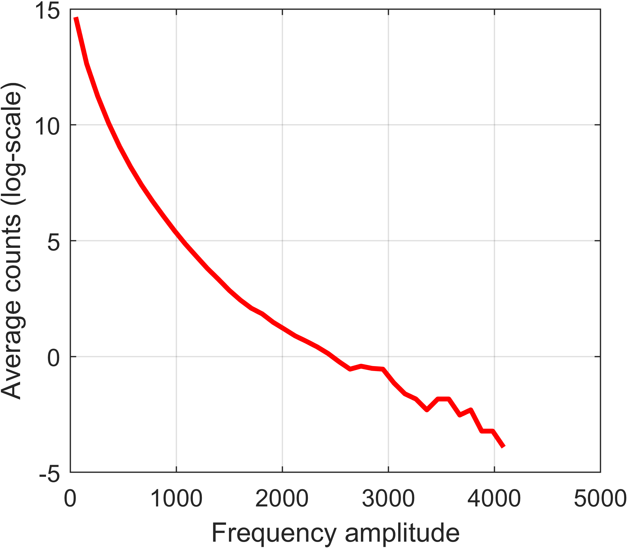
(a) Super-resolution

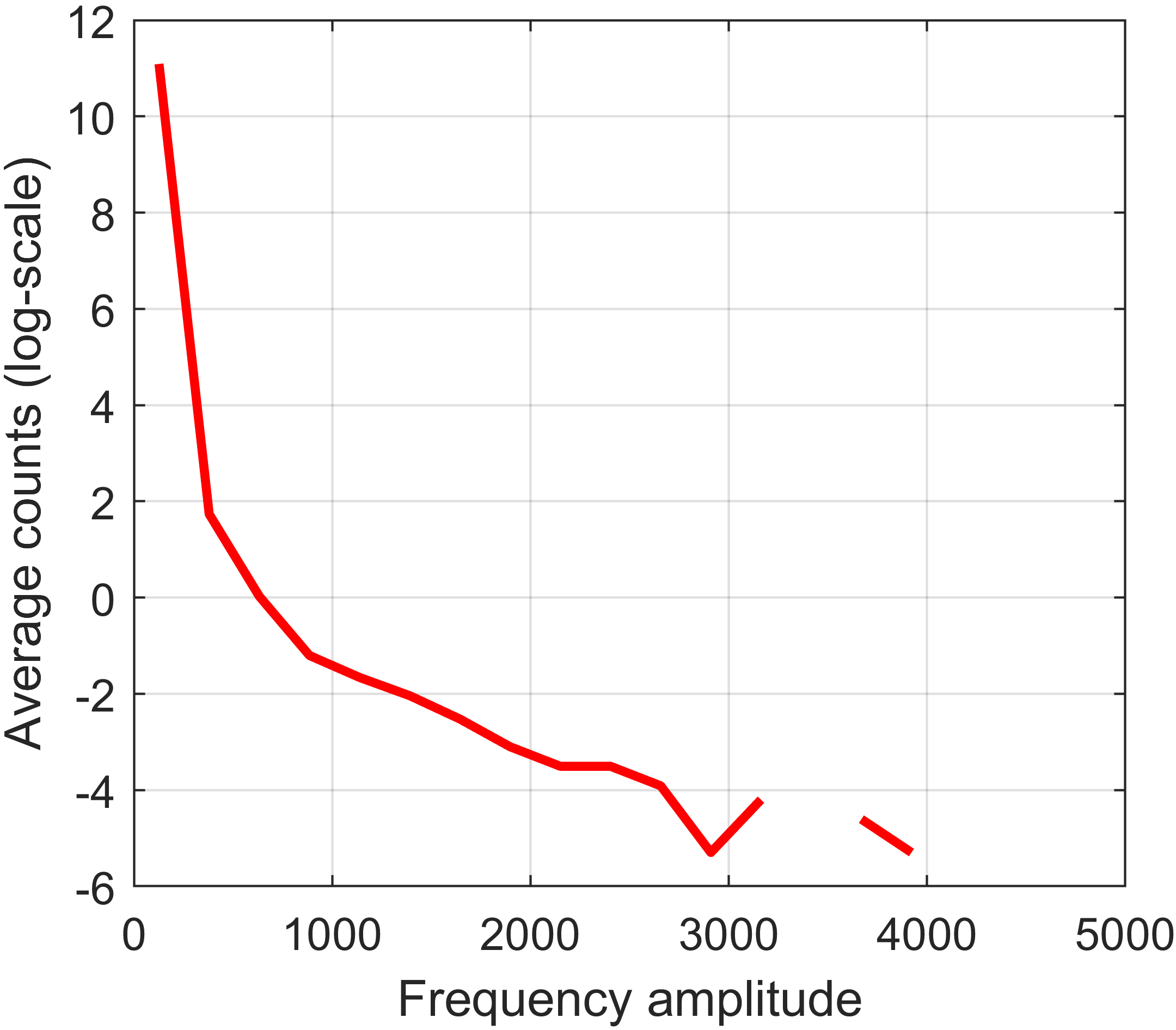
(b) Deraining

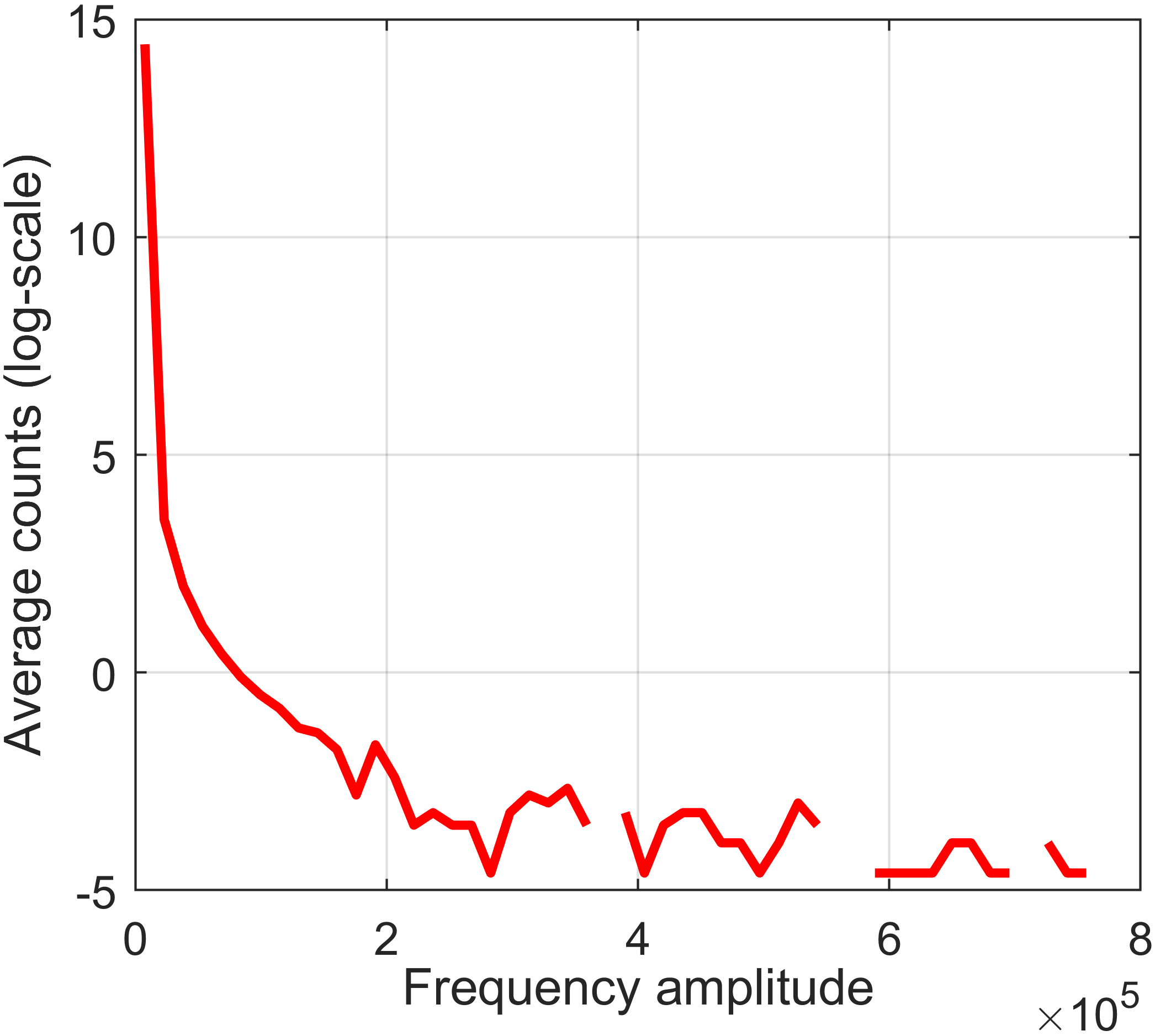
(c) Dehazing

Figure 1: Histograms of the degradation $N$ in the frequency domain for three restoration tasks. (a) Super-resolution (500 real-world images from the RealVSR dataset [85]). (b) Deraining (400 real-world images from the SPA dataset [86]). (c) Dehazing (200 real-world images from the Dense-haze dataset [87]). The degradation in the three tasks are very sparse in the frequency domain, which follows a hyper Laplacian distribution.

In what follows, we show that for three representative restoration tasks, super-resolution, deraining, and dehazing, the degradation $N$ is very sparse in the frequency domain. Fig. 1 presents the histogram statistic of the degradation in the frequency domain for each of the three tasks. 500 real-world images from the super-resolution dataset RealVSR [85], 400 real-world images from the deraining dataset SPA [86], and 200 real-world images from the dehazing dataset Dense-haze [87] are used to compute the histogram statistic for the three tasks, respectively. Given $L$ degraded-clean pairs $\{(y_{i},x_{i})\}_{i=1,\cdots,L}$ from a dataset, the histogram in the frequency domain is computed based on the absolute FFT coefficients $\{|{\rm{fft2}}(y_{i}-x_{i})|\}_{i=1,\cdots,L}$, ${\rm{fft2}}(\cdot)$ is the 2D FFT. Each histogram is averaged over the image pair number $L$. For super-resolution, $Y$ is obtained from a $1/4$ times low resolution version of $X$ by 4 times bicubic up-sampling.

It can be seen from Fig. 1 that, for each of the three tasks, the frequency domain representation of the degradation is very sparse, which follows a hyper-Laplacian distribution. This significant sparsity feature of the degradation provides a natural and useful prior for restoration inference. It is exploited in our method by promoting sparsity of the degradation in the frequency domain to achieve more accurate restoration. Note that although these statistic results are derived based on real-world degradation data, the implementation of our algorithm does not require an accurate estimation of the sparsity parameter of the degradation and, as will be shown in experiments, a rough selection of $q$ of the $\ell_{q}$ cost (e.g. $q\in\{0.5,1\}$) is enough for achieving satisfactory performance.

4.2 Proposed Method Exploiting Degradation Sparsity in OT

The optimal transport criterion (4) does not impose any constraint on the degradation $N$. Though optimal in the case without prior information of the degradation, it is suboptimal when prior information of the degradation is available. For example, if the distribution of $N$ is a priori known, an ideal criterion extending (4) becomes

$$\begin{gathered}\mathop{\min}\limits_{f}{\mathbb{E}_{Y\sim{p_{Y}}}}\left(\left\|f(Y)-Y\right\|^{\beta}\right)\\ {\text{subject \ to \ }}~{}~{}{p_{\hat{X}}}={p_{X}},~{}{p_{\hat{N}}}={p_{N}},\end{gathered}$$ (6)

where $N:=Y-f(Y)=Y-\hat{X}$. Adding the constraint ${p_{\hat{N}}}={p_{N}}$ can effectively leverage the prior information of the degradation process (1) to find a better transport map for the inverse problem $Y\rightarrow X$ with lower distortion. While the distribution $p_{X}$ can be learned from natural clean images, seeking an estimation of $p_{N}$ requires the collection of sufficient degradation $\{n_{i}\}$. In fact, if a collection of sufficient degradation $\{n_{i}\}$ is available, degraded-clean pairs $\{x_{j}+n_{i},x_{j}\}$ can be directly obtained and the restoration model can be learned in a supervised manner. However, in practice, collecting real-world degradation $\{n_{i}\}$ would be as difficult as collecting real-world degraded-clean pairs $\{(y_{i},x_{i})\}$.

In this work, we relax the requirement of $p_{N}$ and employ a simple generic prior for the degradation instead. It is inspired by the above empirical observation that for some restoration tasks the degradation is very sparse in the frequency domain, as shown in Fig. 1. Specifically, we propose a formulation to make use of the frequency domain sparsity of degradation as

$$\begin{gathered}\mathop{\min}\limits_{f}{\mathbb{E}_{Y\sim{p_{Y}}}}\left(\left\|\mathcal{F}(f(Y)-Y)\right\|^{q}_{q}\right)\\ {\text{subject \ to \ }}~{}~{}{p_{\hat{X}}}={p_{X}},\end{gathered}$$ (7)

where $\mathcal{F}(\cdot)$ stands for the discrete Fourier transform, and $\|\cdot\|^{q}_{q}$ is the $\ell_{q}$-norm with $0\leq q\leq 1$. Since the FFT representation of $N$, i.e. $\mathcal{F}(N)$, is sparse, a necessary condition for an inverting map $f$ to be optimal is that it should conform to this property such that $\mathcal{F}(N)=\mathcal{F}(f(Y)-Y)$ is sparse. To achieve this, in formulation (7) we use the $\ell_{q}$-norm loss with $0\leq q\leq 1$ to promote the sparsity. The $\ell_{q}$-norm is a sparsity-promotion loss in data fitting, which has been widely used in sparse recovery to obtain sparse solution [88, 89].

For the particular case of $q=2$, formulation (7) reduces to the OT problem (4) with $\ell_{2}$ cost since $\|\mathcal{F}(f(Y)-Y)\|^{2}_{2}=\|f(Y)-Y\|^{2}_{2}$. The $\ell_{2}$ cost is optimal for degradation with Gaussian distribution but not optimal for sparse degradation with super-Gaussian distribution. As it has been shown in Fig. 1 that, the frequency domain distribution of degradation is far from Gaussian rather being hyper-Laplace, using $\ell_{2}$ cost can result in unsatisfactory performance far from optimal.

In implementation, an unconstrained form of (7) is used as

$$\mathop{\min}\limits_{f}{\mathbb{E}_{Y\sim{p_{Y}}}}\left(\left\|\mathcal{F}(f(Y)-Y)\right\|^{q}_{q}\right)+\lambda d(p_{\hat{X}},p_{X}),$$ (8)

where $\lambda>0$ is a balance parameter. As the discrete Fourier transform is complex-valued, for a vector $M\in\mathbb{C}^{m+1}$, the $\ell_{q}$ loss is computed as

$$\|M\|_{q}^{q}=\sum_{i=0}^{m}\left(\Re^{2}\{M(i)\}+\Im^{2}\{M(i)\}\right)^{\frac{q}{2}}.$$ (9)

4.3 An Analysis on the Effectiveness of the Sparsity Prior

Under the degradation process $Y=X+N$, the distribution of $Y$ is a convolution of the distributions of $X$ and $N$, i.e., $p_{Y}=p_{X}\otimes p_{N}$. Generally, the inverse problem from $Y$ to $X$ is ambiguous due to the information loss in the degradation process. In the absence of any prior information of $N$, the optimal transport map $f_{\sharp}p_{Y}=p_{X}$ obtained by (4) can be used as an ideal inverse (restoration) map [16]. However, when prior information of $N$ is available, the map $f$ is no longer optimal and does not necessarily approach the lower bound of inverse distortion. Naturally, the prior information of $N$ can be exploited to reduce the inverting ambiguity to some extent and hence result in lower restoration distortion.

As our objective is to exploit the underlying sparsity of $N$ to reduce the inverse ambiguity, here we use an example to show the effectiveness of exploiting the sparsity of the degradation in helping to find the desired correct inverse map.

Example 1 [Exploiting the sparsity of degradation helps to find an inverse map with lower distortion]. Consider a discrete random source $X\in\mathbb{R}^{m+1}$, which follows a two-point distribution with probability mass function as

$$p_{X}(x)=\left\{\!{\begin{array}[]{*{20}{l}}\!{p_{1},}&{x=x_{1}}\\ \!{p_{2},}&{x=x_{2}}\end{array}}\right.,$$

with

$$x_{1}=[-a,\mathop{\underbrace{b,\cdots,b}}\limits_{m}]^{T},~{}~{}~{}~{}x_{2}=[-a,\mathop{\underbrace{-b,\cdots,-b}}\limits_{m}]^{T},$$

where $a\gg b>0$ such that $a^{2}>mb^{2}$ and $a^{q}<mb^{q}$ for any $0\leq q\leq 1$. For example, these two conditions hold for $a=1$, $b=0.1$ and $10<m<100$. If only considering $q=0$, they hold for $a=1$, $b=0.1$ and $1<m<100$. Furthermore, consider a degradation process as (1), where $N\in\mathbb{R}^{m+1}$ also follows a two-point distribution with probability mass function given by

$$p_{N}(n)=\left\{\!{\begin{array}[]{*{20}{l}}\!{\tilde{p}_{1},}&{n=n_{1}}\\ \!{\tilde{p}_{2},}&{n=n_{2}}\end{array}}\right.,$$

with

$$n_{1}=[-2a,0,\cdots,0]^{T},~{}~{}~{}~{}n_{2}=[2a,0,\cdots,0]^{T}.$$

Note that $N$ is sparse as only one of its elements is nonzero. In this setting, the distribution of $Y$ is given by the convolution between $p_{X}$ and $p_{N}$ as

$$p_{Y}(y)=\left\{\!{\begin{array}[]{*{20}{l}}\!{p_{1}\tilde{p}_{1},}&{y=y_{1}}\\ \!{p_{1}\tilde{p}_{2},}&{y=y_{2}}\\ \!{p_{2}\tilde{p}_{1},}&{y=y_{3}}\\ \!{p_{2}\tilde{p}_{2},}&{y=y_{4}}\end{array}}\right.,$$

with

$$y_{1}=[-3a,b,\cdots,b]^{T},~{}~{}~{}~{}y_{2}=[a,b,\cdots,b]^{T},$$

$$y_{3}=[-a,-b,\cdots,-b]^{T},~{}~{}~{}~{}y_{4}=[3a,-b,\cdots,-b]^{T}.$$

Then, given the distributions of $X$ and $Y$, we investigate the inverse process $Y\rightarrow X$ by seeking the OT from $p_{Y}$ to $p_{X}$ with different cost functions. Particularly, we evaluate the $\ell_{q}$ cost with $0\leq q\leq 1$ in comparison with the widely used $\ell_{2}$ cost.

First, with the $\ell_{2}$ cost and under the condition $a^{2}>mb^{2}$, a solution $f_{2}^{*}:Y\rightarrow X$ to the OT problem

$$\begin{gathered}\mathop{\min}\limits_{f_{2}}{\mathbb{E}_{Y\sim{p_{Y}}}}\left(\left\|f_{2}(Y)-Y\right\|^{2}_{2}\right)\\ {\text{subject \ to \ }}~{}~{}(f_{2})_{\sharp}{p_{Y}}={p_{X}},\end{gathered}$$ (10)

would map $y_{2}\rightarrow x_{2}$ rather than $y_{2}\rightarrow x_{1}$ since $\|y_{2}-x_{2}\|^{2}_{2}=4mb^{2}<\|y_{3}-x_{2}\|^{2}_{2}=4a^{2}$ and $y_{3}\rightarrow x_{1}$ rather than $y_{3}\rightarrow x_{2}$ since $\|y_{3}-x_{1}\|^{2}_{2}=4mb^{2}<\|y_{3}-x_{2}\|^{2}_{2}=4a^{2}$. For example, let $p_{1}=\tilde{p}_{1}=0.5$ and $p_{2}=\tilde{p}_{2}=0.5$, the optimal map $f_{2}^{*}$ is given by $f_{2}^{*}(y_{1})=x_{1}$, $f_{2}^{*}(y_{2})=x_{2}$, $f_{2}^{*}(y_{3})=x_{1}$, and $f_{2}^{*}(y_{4})=x_{2}$, as illustrated in Fig. 2(b). In contrast, with the $\ell_{q}$ cost and under the condition $a^{q}<mb^{q}$, $\forall q\in[0,1]$, it follows that $\|y_{2}-x_{2}\|^{q}_{q}=m(2b)^{q}>\|y_{3}-x_{2}\|^{q}_{q}=(2a)^{q}$. Hence, the solution $f_{q}^{*}:Y\rightarrow X$ to the OT problem

$$\begin{gathered}\mathop{\min}\limits_{f_{q}}{\mathbb{E}_{Y\sim{p_{Y}}}}\left(\left\|f_{q}(Y)-Y\right\|^{q}_{q}\right)\\ {\text{subject \ to \ }}~{}~{}(f_{q})_{\sharp}{p_{Y}}={p_{X}},\end{gathered}$$ (11)

is given by $f_{q}^{*}(y_{1})=x_{1}$, $f_{q}^{*}(y_{2})=x_{1}$ and $f_{q}^{*}(y_{3})=x_{2}$, $f_{q}^{*}(y_{4})=x_{2}$, as illustrated in Fig. 2(c).

(a) Degradation process

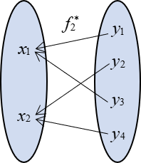
(b) Inverse via OT with $\ell_{2}$ cost

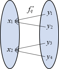
(c) Inverse via OT with $\ell_{q}$ cost for any $0\leq q\leq 1$

Figure 2: An illustration of the optimal transport from $p_{Y}$ to $p_{X}$ with different cost function in Example 1. (a) The degradation process $Y=X+N$. (b) Inverse via the optimal transport $f_{2}$ with $\ell_{2}$ cost. (c) Inverse via the optimal transport $f_{q}$ with $\ell_{q}$ cost for any $0\leq q\leq 1$. In this example, the optimal transport map under the $\ell_{q}$ cost yields the correct inverse map with zero distortion, while that under the $\ell_{2}$ cost does not.

In this example, the residual $N$ is very sparse as it has only one nonzero element. This sparsity property can be exploited by using a sparsity-promotion data fitting cost, such as the $\ell_{q}$-norm with $0\leq q\leq 1$ [88, 89]. Since using the $\ell_{q}$ cost can well exploit the underlying sparsity prior of the degradation to reduce the ambiguity in finding the inverse map, in this example it yields the desired correct inverse map under the OT criterion, which has a zero distortion. In comparison, the $\ell_{2}$ cost yields an undesired map, which does not align with the degradation map and has a nonzero distortion, as shown in Fig. 2. This example illustrates that exploiting the sparsity prior of the degradation (e.g., by the $\ell_{q}$ cost) can effectively help to find an inverse transport map with lower restoration distortion.

5 Experimental Results

We conduct experimental evaluation on three image restoration tasks, including super-resolution, deraining, and dehazing. For each task, the proposed method is compared with state-of-the-art supervised and unsupervised methods on both synthetic and real-world data. Note that, since for each of the tasks there exists a number of supervised and unsupervised methods, it is difficult to compare with all the representative methods in each task. The focus here is to compare with state-of-the-art supervised and unsupervised methods in each task. Particularly, state-of-the-art supervised methods are used as ideal baselines for comparison. For our method, two variants, denoted by SOT ($\ell_{0.5}$) and SOT ($\ell_{1}$), are evaluated in each task, which use the $\ell_{0.5}$ cost and $\ell_{1}$ cost, respectively. The compared methods are as follows.

• For the super-resolution task, the compared supervised methods include RankSR [31], RCAN [32], ESRGAN [30] and RNAN [33]. The compared unsupervised methods include USIS [38], OT[16].

• For the deraining task, the compared methods include DSC[4], RESCAN[43], MPRNet[44], SIRR[45], CycleGAN[35], DeCyGAN[49], OT[16], where DSC is a traditional method, RESCAN and MPRNet are supervised methods, SIRR is a semi-supervised method, while CycleGAN, DeCycleGAN and OT are unsupervised methods.

• For the dehazing task, the compared methods include DCP [5], AODNet [56], Dehamer [57], GCANet [58], FFANet [59], D4 [66], OT [16], where DCP is a traditional model-based method, AODNet, Dehamer, GCANet and FFANet are supervised learning methods, wile D4 and OT are unsupervised learning methods.

In order to make a comprehensive evaluation, the restoration quality is evaluated in terms of both distortion metrics, including peak signal to noise ratio (PSNR) and structural similarity (SSIM), and perceptual quality metrics, including perception index (PI) [90] and learned perceptual image patch similarity (LPIPS) [91].

We implement the proposed formulation (8) based on WGAN-gp [83], with $0\leq q\leq 1$ and $\lambda$ being tuned for each task. Note that the best selection of the value of $q$ depends on the statistics of the data and hence is application and data dependent. In practice it is generally difficult to select the optimal value of $q$. Therefore, in the implementation we only roughly test two values of $q$, e.g., $q=0.5$ and $q=1$ for the $\ell_{q}$ cost of SOT. Experimental results show that this rough selection is sufficient to yield satisfactory performance of SOT.

For a fair comparison, our method and the OT method [16] use the same network structure, which consists of a generator and a discriminator. The generator uses the network in MPRNet [44], which is one of the state-of-the-art models, while the discriminator is the same as that in [16]. The discriminator takes the generator output (restored images) and clean images as input. It should be noted that although clean images are used here, the proposed method is unsupervised because the noisy input of the generator (restoration model) and the clean images input to the discriminator are not paired.

5.1 Synthetic Image Super-Resolution

First, we conduct super-resolution experiment on synthetic data. The used DIV2K[92] dataset contains a total of 1000 high-quality RGB images with a resolution of about 2K. 100 images are used for testing. Since OT requires the input to have the same size as the output, we follow the pre-upsampling method [93] to upsample the low-resolution images before feeding them into the network by bicubic.

TABLE I: Quantitative comparison on 4x super-resolution of synthetic images (using the DIV2K dataset).

Method		PSNR/SSIM	LPIPS/PI
Traditional	Bicubic	26.77/0.755	0.1674/7.07
Supervised	RankSR[31]	26.56/0.734	0.0541/3.01
	RCAN[32]	29.33/0.828	0.0925/5.24
	ESRGAN[30]	26.66/0.749	0.0520/3.26
	RNAN[33]	29.31/0.827	0.0966/5.40
Unsupervised	USIS[38]	22.22/0.628	0.1761/3.52
	OT[16]	25.73/0.719	0.0838/4.44
	SOT ($\ell_{0.5}$)	28.25/0.801	0.0612/3.03
	SOT ($\ell_{1}$)	27.91/0.783	0.0821/3.45

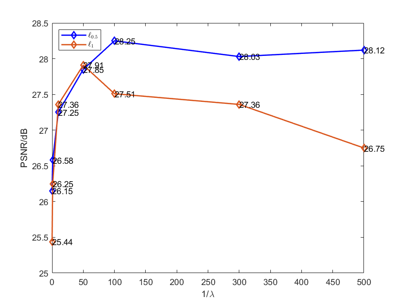
Figure 3: Restoration PSNR of SOT in image super-resolution for different values of $\lambda$.

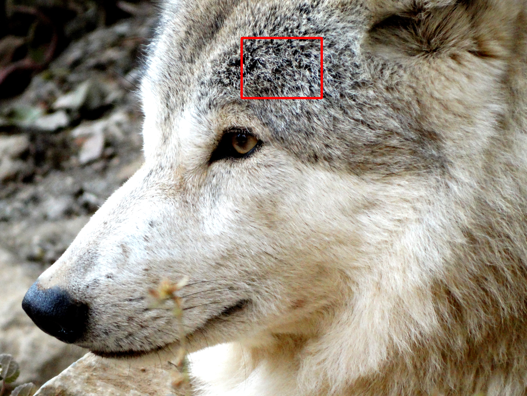
(a) Test image

(b) Ground truth

(c) Bicubic (26.59 dB)

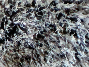
(d) RankSR (26.64/0.743/0.053)

(e) RCAN (29.35/0.829/0.093)

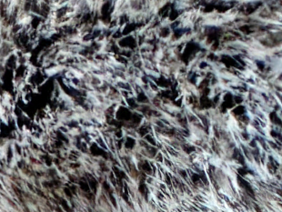
(f) ESRGAN (26.66/0.751/0.052)

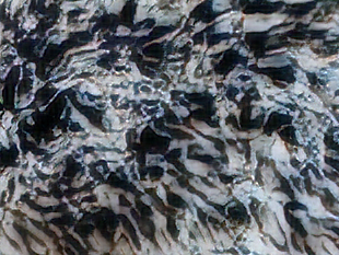
(g) USIS (23.44/0.701/0.167)

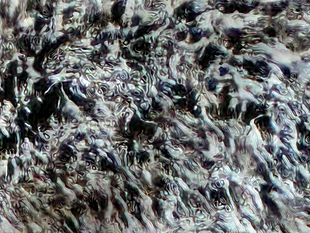
(h) OT (26.88/0.754/0.082)

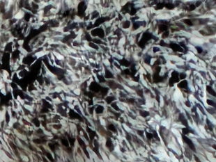
(i) SOT ($\ell_{0.5}$) (28.62/0.821/0.060)

Figure 4: Visual comparison on 4x synthetic image super-resolution. The PSNR/SSIM/LPIPS results are provided in the brackets. The images are enlarged for clarity.

Table 1 presents quantitative results of 4x super-resolution on the DIV2K dataset. It can be seen that the proposed method SOT can achieve PSNR and SSIM results close to those of state-of-the-art supervised learning methods, e.g., with about 1.06 dB difference compared with RCAN. Meanwhile, in terms of the perception indices, its perceptual quality exceeds some of the supervised methods such as RCAN. It should be noted that both RankSR and ESRGAN take perceptual quality as the reconstruction target and use perceptual quality metrics such as LPIPS as the optimization target during training. Hence, they can achieve better perceptual quality scores. However, recent studies on the trade-off between distortion and perceptual quality show that, the improvement in perceptual quality would necessarily lead to increase of reconstruction distortion, e.g. the deterioration of the MSE, PSNR and SSIM metrics [73, 72]. Accordingly, the PSNR and SSIM results of RankSR and ESRGAN are worse. Moreover, by exploiting the degradation sparsity, the proposed SOT significantly outperforms the vanilla OT method, e.g. an improvement of about 2.52 dB in PSNR. Using the $\ell_{0.5}$ cost yields better results of SOT than the $\ell_{1}$ cost.

Fig. 3 shows the PSNR of SOT versus the value of $\lambda$, which investigates the effect of the parameter $\lambda$. Fig. 4 compares the visual quality of 4x super-resolution on a typical sample from the DIV2K dataset. It can be seen that the result of RCAN, which yields the highest PSNR, is closer to the ground-truth, but the reconstructed images appear to be blurred and the details are not clear enough. The proposed SOT method with the $\ell_{0.5}$ cost yields higher PSNR than RankSR and ESRGAN, while having comparable perception quality.

5.2 Real-Word Image Super-Resolution

TABLE II: Quantitative comparison on real-world image super-resolution (using the RealVSR dataset).

Method		PSNR/SSIM	LPIPS/PI
Traditional	Bicubic	23.15/0.749	0.1347/5.94
Supervised	RankSR[31]	21.05/0.607	0.1031/2.79
	RCAN[32]	23.39/0.772	0.1573/5.79
	ESRGAN[30]	21.13/0.632	0.1024/3.53
	RNAN[33]	23.19/0.752	0.1599/5.88
Unsupervised	USIS[38]	19.06/0.502	0.2122/3.35
	OT[16]	21.34/0.658	0.1110/4.12
	SOT ($\ell_{0.5}$)	23.89/0.782	0.0839/3.27
	SOT ($\ell_{1}$)	22.85/0.722	0.0758/3.23

In synthetic super-resolution experiments, bicubic down-sampling is widely used to construct paired training data. However, real-word degradation can substantially deviate from bicubic down-sampling. This limits the performance of the synthetic data learned model on real-world data. To further verify the performance of the proposed method on real scenes, we conduct experiment on a real-world super-resolution dataset RealVSR [85]. In this dataset, paired data is constructed by firstly using the multi-camera system of iPhone 11 Pro Max to capture images of different resolutions in the same scene separately, and then adopting post-processing such as color correction and pixel alignment. The results on this dataset are shown in Table 2.

(a) Test image

(b) Ground truth

(c) bicubic (23.01 dB)

(d) RankSR (20.87/0.612/0.104)

(e) RCAN (23.48/0.784/0.157)

(f) ESRGAN (21.06/0.634/0.101)

(g) USIS (19.57/0.527/0.211)

(h) OT (21.65/0.674/0.111)

(i) SOT ($\ell_{0.5}$) (24.03/0.792/0.084)

Figure 5: Visual comparison on real-world image super-resolution. The PSNR/SSIM/LPIPS results are provided in the brackets. The images are enlarged for clarity.

From the results, the proposed method can achieve better PSNR, SSIM and LPIPS scores even compared with state-of-the-art supervised methods. Moreover, exploiting degradation sparsity can improve the performance of the OT method by a large margin. For example, SOT($\ell_{0.5}$) achieves a PSNR about 2.55 dB higher than OT with significant better perception scores. SOT($\ell_{0.5}$) has lower distortion than SOT($\ell_{1}$) (e.g. about 1 dB higher in PSNR) but with worse perception scores. This accords well with the distortion-perception tradeoff theory.

Fig. 5 compares the visual quality of the methods on a typical sample from the RealVSR dataset. It can be seen that SOT achieves the best PSNR, SSIM and LPIPS scores. Qualitatively, it can achieve high-quality detail reconstruction while having less artifacts than the perception-oriented methods.

5.3 Synthetic Image Deraining

For synthetic image deraining, we train the models on the Rain1800 dataset [94] and test on the Rain100L dataset [95]. These two datasets respectively contain 1800 and 100 images of natural scenes with simulated raindrops.

TABLE III: Quantitative comparison of the deraining methods on synthetic data (the Rain1800 and Rain100L datasets are used for training and testing, respectively).

method		PSNR/SSIM	LPIPS/PI
	Rainy	25.52/0.825	0.1088/3.77
Traditional	DSC[4]	25.72/0.831	0.1116/2.79
	RESCAN[43]	29.80/0.881	0.0731/2.87
Supervised	MPRNet[44]	36.40/0.965	0.0167/3.21
Semi-supervised	SIRR[45]	23.48/0.800	0.0978/2.88
	CycleGAN[35]	24.03/0.820	0.0960/2.80
	DeCyGAN[49]	24.89/0.821	0.0952/3.12
	OT[16]	33.71/0.954	0.0158/2.76
	SOT ($\ell_{0.5}$)	34.74/0.948	0.0132/2.54
Unsupervised	SOT ($\ell_{1}$)	35.33/0.963	0.0108/2.51

Table 3 shows the quantitative results tested on the Rain100 dataset. Clearly, the proposed method can achieve a PSNR close to the state-of-the-art supervised method. For example, the difference in PSNR between SOT($\ell_{1}$) and MPRNet is about 1.07 dB. Noteworthily, SOT($\ell_{1}$) achieves the best perception scores among all the compared unsupervised and supervised methods. Again, SOT performs much better than OT, which demonstrates the effectiveness sparsity exploitation. For SOT, the $\ell_{1}$ cost yields better performance than the $\ell_{0.5}$ cost.

(a) Test image

(b) Ground truth

(c) Rainy (25.41 dB)

(d) DSC (25.78/0.835/0.112)

(e) RESCAN (30.21/0.892/0.072)

(f) MPRNet (36.58/0.972/0.018)

(g) SIRR (24.59/0.825/0.098)

(h) DeCyGAN (25.32/0.865/0.095)

(i) SOT ($\ell_{1}$) (36.02/0.968/0.011)

Figure 6: Visual comparison on synthetic image deraining. The PSNR/SSIM/LPIPS results are provided in the brackets. The images are enlarged for clarity.

Fig. 6 compares the visual quality of the methods. It can be observed that the supervised methods, such as MPRNet, can achieve excellent rain removal but with the restoration being over-smoothing. The proposed method can reconstruct better texture details, while achieving effective rain removal.

TABLE IV: Quantitative comparison of the deraining methods on real-world data (using the SPA dataset [86]).

method		PSNR/SSIM	LPIPS/PI
	Rainy	34.30/0.923	0.0473/8.49
Traditional	DSC[4]	32.29/0.921	0.0498/7.89
	RESCAN[43]	38.34/0.961	0.0250/8.03
Supervised	MPRNet[44]	46.12/0.986	0.0109/7.68
Semi-supervised	SIRR[45]	22.66/0.710	0.1323/7.87
	CycleGAN[35]	28.79/0.923	0.0422/7.58
	DeCyGAN[49]	34.78/0.929	0.0528/7.50
	OT[16]	41.68/0.951	0.0098/7.35
	SOT ($\ell_{0.5}$)	42.69/0.958	0.0096/7.15
Unsupervised	SOT ($\ell_{1}$)	44.37/0.982	0.0084/7.06

5.4 Real-world Image Deraining

For the real-world image derainging experiment, we chose the real scene dataset SPA [86] for training and testing. This dataset takes images with and without rain in the same scene by fixing the camera position, hence the rain-free images can be used as the ground-truth for supervised model training. The experimental results are shown in Table 4.

Similar to the results in the synthetic deraining experiment, the proposed method achieves the best performance among the unsupervised methods. It achieves a PSNR only 1.75 dB lower than the state-of-the-art supervised method MPRNet. Particularly, SOT achieves the best perception scores, which even surpasses that of the supervised methods. In addition, SOT($\ell_{1}$) attains a PSNR 2.69 dB higher than that of the vanilla OT method.

(a) Ground truth

(b) Rainy (35.26 dB)

(c) DSC (32.36/0.915/0.050)

(d) RESCAN (38.65/0.962/0.024)

(e) MPRNet (45.62/0.982/0.011)

(f) SIRR (22.31/0.689/0.132)

(g) CycleGAN (30.27/0.856/0.040)

(h) DeCyGAN (34.58/0.918/0.053)

(i) SOT ($\ell_{1}$) (45.72/0.979/0.008)

Figure 7: Visual comparison on real-world image deraining. The PSNR/SSIM/LPIPS results are provided in the brackets.

Fig. 7 compares the visual quality of the deraining methods on a typical real sample. It can be seen that, SOT can achieve a quality on par with the state-of-the-art supervised method MPRNet to provide a visually plausible restoration, which demonstrate the effectiveness of SOT on real data. It should be noted that although CycleGAN can also achieve excellent rain removal, it introduces additional distortion such as color, resulting in larger distortion, e.g., with a PSNR more than 10 dB lower than that of MPRNet and SOT.

5.5 Synthetic Image Dehazing

Hazy scenes, like rainy scenes, can significantly affect the quality of the captured images, but the difference in distribution between the two is obvious. Under a hazy sky, the whole image will be covered with a gray or white fog layer. Therefore, a global image reconstruction is needed. For the synthetic image dehazing task, we train and test the models on the OTS dataset [96]. This dataset contains a large number of images of outdoor scenes with various levels of synthetic fog layers. We selected 100 images from the dataset as the test set.

Table 5 shows the quantitative results of the compared methods on the OTS dataset. It can be seen that the proposed method can achieve a PSNR approaching that of the state-of-the-art supervised methods. For instance, the difference in PSNR between SOT($\ell_{1}$) and the state-of-the-art transformer based supervised method Dehamer is about 1.18 dB, while SOT($\ell_{1}$) achieves the best perception scores among all the compared supervised and unsupervised methods. In this experiment, SOT with the $\ell_{1}$ cost attains a PSNR 3.37 dB higher than the standard OT method, e.g., 32.20 dB versus 28.83 dB. Fig. 8 compares the visual quality of the methods. The restoration quality of the proposed method is even on par with Dehamer.

TABLE V: Quantitative comparison of the dehazing methods on synthetic data (using the OTS dataset [96]).

Method		PSNR/SSIM	LPIPS/PI
	Hazy	18.13/0.851	0.0747/2.96
Traditional	DCP[5]	16.83/0.863	0.0670/2.27
	AODNet[56]	18.42/0.828	0.0703/2.69
	Dehamer[57]	33.38/0.946	0.0168/2.35
	GCANet[58]	19.85/0.704	0.0689/2.39
Supervised	FFANet[59]	30.80/0.935	0.0182/2.68
	D4[66]	21.89/0.845	0.0466/2.39
	OT[16]	28.83/0.919	0.0236/2.60
	SOT ($\ell_{0.5}$)	31.63/0.905	0.0165/2.14
Unsupervised	SOT ($\ell_{1}$)	32.20/0.935	0.0157/2.08

(a) Test image

(b) Ground truth

(c) Hazy (20.72 dB)

(d) DCP (18.23/0.851/0.067)

(e) Dehamer (34.62/0.953/0.017)

(f) GCANet (21.69/0.756/0.070)

(g) FFANet (32.81/0.936/0.019)

(h) D4 (21.98/0.864/0.047)

(i) SOT ($\ell_{1}$) (34.57/0.914/0.016)

Figure 8: Visual comparison on synthetic image dehazing. The PSNR/SSIM/LPIPS results are provided in the brackets. The images are enlarged for clarity.

5.6 Real-World Image Dehazing

For the real-world image dahazing task, we chose the real scene dataset Dense-haze [87] for training and testing. This dataset was obtained from two sets of images in the same scene with fog and under normal conditions through artificial smoke. The artificial smoke in the dataset is quite dense and hence the restoration task is extremely challenging.

TABLE VI: Quantitative comparison of the compared methods on real-world data (using hteDense-haze dataset [87]).

Method		PSNR/SSIM	LPIPS/PI
	Hazy	10.55/0.435	0.2057/7.04
Traditional	DCP[5]	11.01/0.415	0.3441/5.91
	AODNet[56]	10.64/0.469	0.2453/6.11
	Dehamer[57]	16.63/0.585	0.1523/5.65
	GCANet[58]	12.46/0.454	0.2524/5.04
Supervised	FFANet[59]	8.77/0.452	0.1985/6.71
	D4[66]	9.69/0.462	0.2140/5.03
	OT[16]	14.17/0.503	0.1699/4.89
	SOT ($\ell_{0.5}$)	15.01/0.526	0.1523/4.56
Unsupervised	SOT ($\ell_{1}$)	15.40/0.567	0.1451/4.50

Table 6 presents the results of the compared methods on this dataset. Similar to the results in the synthetic dehazing task, SOT achieves the best performance among the unsupervised methods. Besides, in term of the LPIPS and PI scores, its perception quality even surpasses that of the supervised methods, i.e. the best among all the compared supervised and unsupervised methods. Compared with the standard OT method, the performance of SOT still improves considerably on this challenging realistic task.

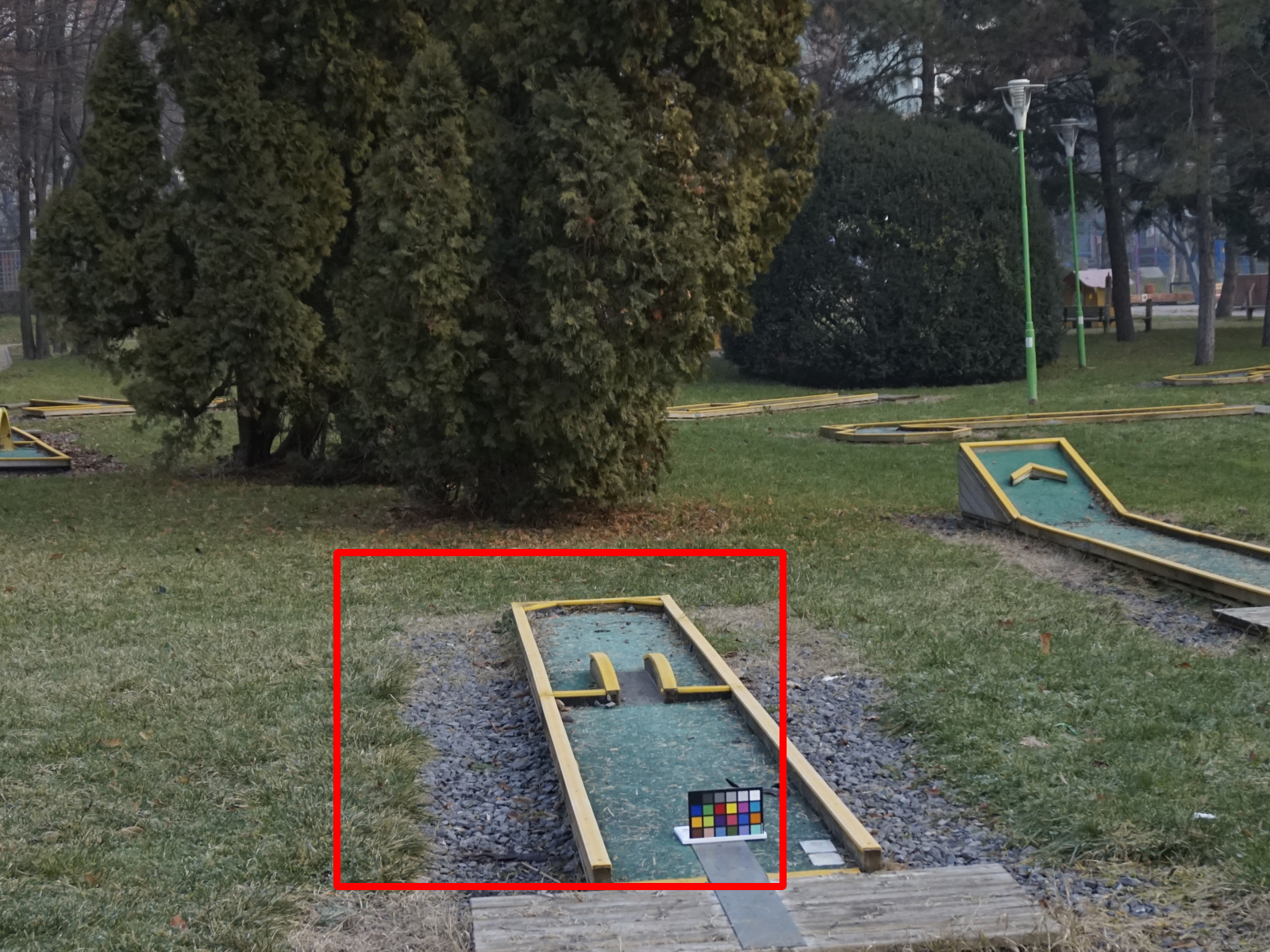
(a) Test image

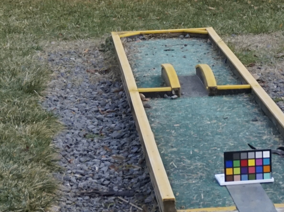
(b) Ground truth

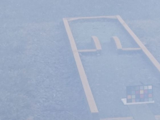
(c) Hazy (9.89 dB)

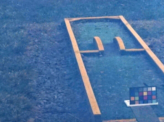
(d) DCP (10.35/0.407/0.342)

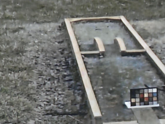
(e) Dehamer (15.87/0.569/0.155)

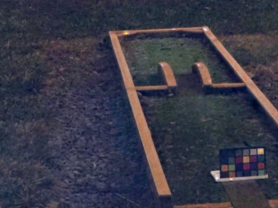
(f) GCANet (13.62/0.487/0.256)

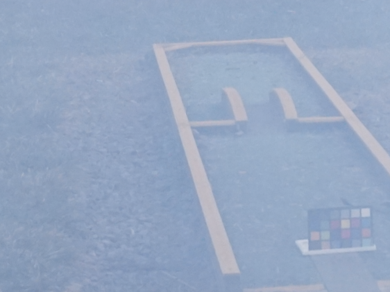
(g) FFANet (8.61/0.464/0.199)

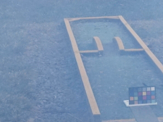
(h) D4 (9.77/0.471/0.217)

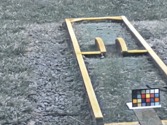
(i) SOT ($\ell_{1}$) (14.78/0.536/0.146)

Figure 9: Visual comparison on a challenging real-word image dehazing task with severe haze. The PSNR/SSIM/LPIPS results are provided in the brackets. The images are enlarged for clarity.

Fig. 9 compares the visual quality of the methods. Noteworthily, the visual quality of SOT is distinctly better compared with the state-of-the-art transformer based supervised method Dehamer, e.g. the color of the palette restored by SOT is much closer to the real scene. This task is quite challenging as the observation (hazy images) is severely degraded with an average PSNR of only about 10 dB. The results demonstrate the potential of the proposed method on realistic difficult tasks to handle complex degradation.

6 Conclusions

An unsupervised restoration learning method has been developed, which exploits the sparsity of degradation in the OT criterion to reduce the ambiguity in seeking an inverse map for the restoration problem. It is based on an observation that, the degradation for some restoration tasks is sparse in the frequency domain. The proposed method has been extensively evaluated in comparison with existing supervised and unsupervised methods on super-resolution, deraining, and dehazing tasks. The results demonstrate that it can significantly improve the performance of the OT criterion to approach the performance of state-of-the-art supervised methods. Particularly, among the compared supervised and unsupervised methods, the proposed method achieves the best PSNR, SSIM and LPIPS results in real-world super-resolution, and the best perception scores (LPIPS and PI) in real-world deraining and dehazing. Our method is the first generic unsupervised method that can achieve favorable performance in comparison with state-of-the-art supervised methods on all the super-resolution, deraining, and dehazing tasks.

References

- [1] A. Buades, B. Coll, and J.-M. Morel, “A non-local algorithm for image denoising,” in IEEE Conference Computer Vision and Pattern Recognition (CVPR), vol. 2, pp. 60–65, 2005.
- [2] K. Dabov, A. Foi, V. Katkovnik, and K. Egiazarian, “Image denoising by sparse 3-d transform-domain collaborative filtering,” IEEE Transactions on Image Processing, vol. 16, no. 8, pp. 2080–2095, 2007.
- [3] M. Elad and A. Feuer, “Restoration of a single superresolution image from several blurred, noisy, and undersampled measured images,” IEEE Transactions on Image Processing, vol. 6, no. 12, pp. 1646–1658, 1997.
- [4] Y. Luo, Y. Xu, and H. Ji, “Removing rain from a single image via discriminative sparse coding,” in IEEE/CVF International Conference on Computer Vision, pp. 3397–3405, 2015.
- [5] K. He, J. Sun, and X. Tang, “Single image haze removal using dark channel prior,” IEEE Transactions on Pattern Analysis and Machine Intelligence, vol. 33, no. 12, pp. 2341–2353, 2010.
- [6] X. Mao, C. Shen, and Y.-B. Yang, “Image restoration using very deep convolutional encoder-decoder networks with symmetric skip connections,” in Advances in Neural Information Processing Systems, pp. 2802–2810, 2016.
- [7] Y. Zhang, Y. Tian, Y. Kong, B. Zhong, and Y. Fu, “Residual dense network for image restoration,” IEEE Transactions on Pattern Analysis and Machine Intelligence, vol. 43, no. 7, pp. 2480–2495, 2020.
- [8] J. Lehtinen, J. Munkberg, J. Hasselgren, S. Laine, T. Karras, M. Aittala, and T. Aila, “Noise2noise: Learning image restoration without clean data,” in International Conference on Machine Learning (ICML), pp. 4620–4631, 2018.
- [9] A. Krull, T.-O. Buchholz, and F. Jug, “Noise2void-learning denoising from single noisy images,” in IEEE Conference Computer Vision and Pattern Recognition (CVPR), pp. 2129–2137, 2019.
- [10] J. Batson and L. Royer, “Noise2self: Blind denoising by self-supervision,” in International Conference on Machine Learning (ICML), pp. 524–533, 2019.
- [11] T. Ehret, A. Davy, J.-M. Morel, G. Facciolo, and P. Arias, “Model-blind video denoising via frame-to-frame training,” in IEEE Conference Computer Vision and Pattern Recognition (CVPR), pp. 11369–11378, 2019.
- [12] Y. Quan, M. Chen, T. Pang, and H. Ji, “Self2self with dropout: Learning self-supervised denoising from single image,” in IEEE Conference Computer Vision and Pattern Recognition (CVPR), pp. 1890–1898, 2020.
- [13] M. Zhussip, S. Soltanayev, and S. Y. Chun, “Extending stein’s unbiased risk estimator to train deep denoisers with correlated pairs of noisy images,” in Advances in Neural Information Processing Systems, pp. 1465–1475, 2019.
- [14] S. Laine, T. Karras, J. Lehtinen, and T. Aila, “High-quality self-supervised deep image denoising,” Advances in Neural Information Processing Systems, vol. 32, pp. 6970–6980, 2019.
- [15] X. Wu, M. Liu, Y. Cao, D. Ren, and W. Zuo, “Unpaired learning of deep image denoising,” in European Conference on Computer Vision (ECCV), pp. 352–368, 2020.
- [16] W. Wang, F. Wen, Z. Yan, and P. Liu, “Optimal transport for unsupervised denoising learning,” IEEE Transactions on Pattern Analysis and Machine Intelligence, vol. 45, no. 2, pp. 2104–2118, 2023.
- [17] A. Buades, B. Coll, and J.-M. Morel, “A review of image denoising algorithms, with a new one,” Multiscale Modeling & Simulation, vol. 4, no. 2, pp. 490–530, 2005.
- [18] M. Lebrun, “An analysis and implementation of the bm3d image denoising method,” Image Processing on Line, vol. 2012, pp. 175–213, 2012.
- [19] N. Moran, D. Schmidt, Y. Zhong, and P. Coady, “Noisier2noise: Learning to denoise from unpaired noisy data,” in IEEE Conference Computer Vision and Pattern Recognition (CVPR), pp. 12064–12072, 2020.
- [20] J. Xu, Y. Huang, M.-M. Cheng, L. Liu, F. Zhu, Z. Xu, and L. Shao, “Noisy-as-clean: learning self-supervised denoising from corrupted image,” IEEE Transactions on Image Processing, vol. 29, pp. 9316–9329, 2020.
- [21] S. Cha, T. Park, B. Kim, J. Baek, and T. Moon, “Gan2gan: Generative noise learning for blind denoising with single noisy images,” in International Conference on Learning Representations, 2020.
- [22] S. Soltanayev and S. Y. Chun, “Training deep learning based denoisers without ground truth data,” in Advances in Neural Information Processing Systems, pp. 3261–3271, 2018.
- [23] A. Krull, T. Vičar, M. Prakash, M. Lalit, and F. Jug, “Probabilistic noise2void: Unsupervised content-aware denoising,” Frontiers in Computer Science, vol. 2, p. 5, 2020.
- [24] R. Tsai, “Multiframe image restoration and registration,” Advance Computer Visual and Image Processing, vol. 1, pp. 317–339, 1984.
- [25] R. R. Schultz and R. L. Stevenson, “Extraction of high-resolution frames from video sequences,” IEEE Transactions on Image Processing, vol. 5, no. 6, pp. 996–1011, 1996.
- [26] D. Glasner, S. Bagon, and M. Irani, “Super-resolution from a single image,” in IEEE International Conference on Computer Vision, pp. 349–356, 2009.
- [27] C. Dong, C. C. Loy, K. He, and X. Tang, “Image super-resolution using deep convolutional networks,” IEEE Transactions on Pattern Analysis and Machine Intelligence, vol. 38, no. 2, pp. 295–307, 2015.
- [28] J. Kim, J. K. Lee, and K. M. Lee, “Accurate image super-resolution using very deep convolutional networks,” in IEEE Conference on Computer Vision and Pattern Recognition, pp. 1646–1654, 2016.
- [29] C. Ledig, L. Theis, F. Huszár, J. Caballero, A. Cunningham, A. Acosta, A. Aitken, A. Tejani, J. Totz, Z. Wang, et al., “Photo-realistic single image super-resolution using a generative adversarial network,” in IEEE Conference on Computer Vision and Pattern Recognition, pp. 4681–4690, 2017.
- [30] X. Wang, K. Yu, S. Wu, J. Gu, Y. Liu, C. Dong, Y. Qiao, and C. Change Loy, “Esrgan: Enhanced super-resolution generative adversarial networks,” in European Conference on Computer Vision (ECCV) Workshops, 2018.
- [31] W. Zhang, Y. Liu, C. Dong, and Y. Qiao, “Ranksrgan: Generative adversarial networks with ranker for image super-resolution,” in IEEE/CVF International Conference on Computer Vision, pp. 3096–3105, 2019.
- [32] Y. Zhang, K. Li, K. Li, L. Wang, B. Zhong, and Y. Fu, “Image super-resolution using very deep residual channel attention networks,” in European Conference on Computer Vision (ECCV), pp. 286–301, 2018.
- [33] Y. Zhang, K. Li, K. Li, B. Zhong, and Y. Fu, “Residual non-local attention networks for image restoration,” in International Conference on Learning Representations (ICLR), 2018.
- [34] I. Goodfellow, J. Pouget-Abadie, M. Mirza, B. Xu, D. Warde-Farley, S. Ozair, A. Courville, and Y. Bengio, “Generative adversarial nets,” in Advances in Neural Information Processing Systems, 2014.
- [35] J.-Y. Zhu, T. Park, P. Isola, and A. A. Efros, “Unpaired image-to-image translation using cycle-consistent adversarial networks,” in IEEE/CVF International Conference on Computer Vision, pp. 2223–2232, 2017.
- [36] A. Lugmayr, M. Danelljan, and R. Timofte, “Unsupervised learning for real-world super-resolution,” in IEEE/CVF International Conference on Computer Vision Workshop (ICCVW), pp. 3408–3416, 2019.
- [37] Y. Yuan, S. Liu, J. Zhang, Y. Zhang, C. Dong, and L. Lin, “Unsupervised image super-resolution using cycle-in-cycle generative adversarial networks,” in IEEE Conference on Computer Vision and Pattern Recognition Workshops, pp. 701–710, 2018.
- [38] K. Prajapati, V. Chudasama, H. Patel, K. Upla, R. Ramachandra, K. Raja, and C. Busch, “Unsupervised single image super-resolution network (usisresnet) for real-world data using generative adversarial network,” in IEEE/CVF Conference on Computer Vision and Pattern Recognition (CVPR) Workshops, pp. 464–465, 2020.
- [39] A. Bulat, J. Yang, and G. Tzimiropoulos, “To learn image super-resolution, use a gan to learn how to do image degradation first,” in European Conference on Computer Vision (ECCV), pp. 185–200, 2018.
- [40] T. Zhao, W. Ren, C. Zhang, D. Ren, and Q. Hu, “Unsupervised degradation learning for single image super-resolution,” arXiv preprint arXiv:1812.04240, 2018.
- [41] L. Wang, Y. Wang, X. Dong, Q. Xu, J. Yang, W. An, and Y. Guo, “Unsupervised degradation representation learning for blind super-resolution,” in IEEE/CVF Conference on Computer Vision and Pattern Recognition, pp. 10581–10590, 2021.
- [42] N. Ahn, J. Yoo, and K.-A. Sohn, “Simusr: A simple but strong baseline for unsupervised image super-resolution,” in IEEE/CVF Conference on Computer Vision and Pattern Recognition Workshops, pp. 474–475, 2020.
- [43] X. Li, J. Wu, Z. Lin, H. Liu, and H. Zha, “Recurrent squeeze-and-excitation context aggregation net for single image deraining,” in European Conference on Computer Vision (ECCV), pp. 254–269, 2018.
- [44] S. W. Zamir, A. Arora, S. Khan, M. Hayat, F. S. Khan, M.-H. Yang, and L. Shao, “Multi-stage progressive image restoration,” in IEEE Conference Computer Vision and Pattern Recognition (CVPR), pp. 14821–14831, 2021.
- [45] W. Wei, D. Meng, Q. Zhao, Z. Xu, and Y. Wu, “Semi-supervised transfer learning for image rain removal,” in IEEE Conference on Computer Vision and Pattern Recognition (CVPR), pp. 3877–3886, 2019.
- [46] X. Fu, J. Huang, X. Ding, Y. Liao, and J. Paisley, “Clearing the skies: A deep network architecture for single-image rain removal,” IEEE Transactions on Image Processing, vol. 26, no. 6, pp. 2944–2956, 2017.
- [47] R. Li, L.-F. Cheong, and R. T. Tan, “Heavy rain image restoration: Integrating physics model and conditional adversarial learning,” in IEEE/CVF Conference on Computer Vision and Pattern Recognition, pp. 1633–1642, 2019.
- [48] M. Mirza and S. Osindero, “Conditional generative adversarial nets,” arXiv preprint arXiv:1411.1784, 2014.
- [49] Y. Wei, Z. Zhang, Y. Wang, M. Xu, Y. Yang, S. Yan, and M. Wang, “Deraincyclegan: Rain attentive cyclegan for single image deraining and rainmaking,” IEEE Transactions on Image Processing, vol. 30, pp. 4788–4801, 2021.
- [50] X. Jin, Z. Chen, J. Lin, Z. Chen, and W. Zhou, “Unsupervised single image deraining with self-supervised constraints,” in IEEE International Conference on Image Processing (ICIP), pp. 2761–2765, 2019.
- [51] H. Zhu, X. Peng, J. T. Zhou, S. Yang, V. Chanderasekh, L. Li, and J.-H. Lim, “Singe image rain removal with unpaired information: A differentiable programming perspective,” in Proceedings of the AAAI Conference on Artificial Intelligence, vol. 33, pp. 9332–9339, 2019.
- [52] Y. Ye, C. Yu, Y. Chang, L. Zhu, X.-l. Zhao, L. Yan, and Y. Tian, “Unsupervised deraining: Where contrastive learning meets self-similarity,” in IEEE/CVF Conference on Computer Vision and Pattern Recognition, pp. 5821–5830, 2022.
- [53] R. Fattal, “Single image dehazing,” ACM Transactions on Graphics (TOG), vol. 27, no. 3, pp. 1–9, 2008.
- [54] A. Golts, D. Freedman, and M. Elad, “Unsupervised single image dehazing using dark channel prior loss,” IEEE Transactions on Image Processing, vol. 29, pp. 2692–2701, 2019.
- [55] B. Cai, X. Xu, K. Jia, C. Qing, and D. Tao, “Dehazenet: An end-to-end system for single image haze removal,” IEEE Transactions on Image Processing, vol. 25, no. 11, pp. 5187–5198, 2016.
- [56] B. Li, X. Peng, Z. Wang, J. Xu, and D. Feng, “Aod-net: All-in-one dehazing network,” in IEEE/CVF International Conference on Computer Vision, pp. 4770–4778, 2017.
- [57] C.-L. Guo, Q. Yan, S. Anwar, R. Cong, W. Ren, and C. Li, “Image dehazing transformer with transmission-aware 3d position embedding,” in IEEE Conference on Computer Vision and Pattern Recognition (CVPR), pp. 5812–5820, 2022.
- [58] D. Chen, M. He, Q. Fan, J. Liao, L. Zhang, D. Hou, L. Yuan, and G. Hua, “Gated context aggregation network for image dehazing and deraining,” in IEEE Winter Conference on Applications of Computer Vision (WACV), pp. 1375–1383, 2019.
- [59] X. Qin, Z. Wang, Y. Bai, X. Xie, and H. Jia, “Ffa-net: Feature fusion attention network for single image dehazing,” in AAAI Conference on Artificial Intelligence, vol. 34, pp. 11908–11915, 2020.
- [60] X. Yang, Z. Xu, and J. Luo, “Towards perceptual image dehazing by physics-based disentanglement and adversarial training,” in AAAI Conference on Artificial Intelligence, vol. 32, 2018.
- [61] S. Zhao, L. Zhang, Y. Shen, and Y. Zhou, “Refinednet: A weakly supervised refinement framework for single image dehazing,” IEEE Transactions on Image Processing, vol. 30, pp. 3391–3404, 2021.
- [62] A. Dudhane and S. Murala, “Cdnet: Single image de-hazing using unpaired adversarial training,” in IEEE Winter Conference on Applications of Computer Vision (WACV), pp. 1147–1155, IEEE, 2019.
- [63] D. Engin, A. Genç, and H. Kemal Ekenel, “Cycle-dehaze: Enhanced cyclegan for single image dehazing,” in IEEE Conference on Computer Vision and Pattern Recognition Workshops, pp. 825–833, 2018.
- [64] J. Zhao, J. Zhang, Z. Li, J.-N. Hwang, Y. Gao, Z. Fang, X. Jiang, and B. Huang, “Dd-cyclegan: Unpaired image dehazing via double-discriminator cycle-consistent generative adversarial network,” Engineering Applications of Artificial Intelligence, vol. 82, pp. 263–271, 2019.
- [65] W. Liu, X. Hou, J. Duan, and G. Qiu, “End-to-end single image fog removal using enhanced cycle consistent adversarial networks,” IEEE Transactions on Image Processing, vol. 29, pp. 7819–7833, 2020.
- [66] Y. Yang, C. Wang, R. Liu, L. Zhang, X. Guo, and D. Tao, “Self-augmented unpaired image dehazing via density and depth decomposition,” in IEEE Conference on Computer Vision and Pattern Recognition (CVPR), pp. 2037–2046, 2022.
- [67] Z. Wang, G. Wu, H. R. Sheikh, E. P. Simoncelli, E.-H. Yang, and A. C. Bovik, “Quality-aware images,” IEEE Transactions on Image Processing, vol. 15, no. 6, pp. 1680–1689, 2006.
- [68] A. Mittal, A. K. Moorthy, and A. C. Bovik, “No-reference image quality assessment in the spatial domain,” IEEE Transactions on Image Processing, vol. 21, no. 12, pp. 4695–4708, 2012.
- [69] A. K. Moorthy and A. C. Bovik, “Blind image quality assessment: From natural scene statistics to perceptual quality,” IEEE Transactions on Image Processing, vol. 20, no. 12, pp. 3350–3364, 2011.
- [70] M. A. Saad, A. C. Bovik, and C. Charrier, “Blind image quality assessment: A natural scene statistics approach in the dct domain,” IEEE Transactions on Image Processing, vol. 21, no. 8, pp. 3339–3352, 2012.
- [71] Y. Blau and T. Michaeli, “The perception-distortion tradeoff,” in IEEE Conference Computer Vision and Pattern Recognition (CVPR), pp. 6228–6237, 2018.
- [72] Z. Yan, F. Wen, R. Ying, C. Ma, and P. Liu, “On perceptual lossy compression: The cost of perceptual reconstruction and an optimal training framework,” in International Conference on Machine Learning (ICML), pp. 11682–11692, 2021.
- [73] Y. Blau and T. Michaeli, “Rethinking lossy compression: The rate-distortion-perception tradeoff,” in International Conference on Machine Learning (ICML), pp. 675–685, 2019.
- [74] Z. Yan, F. Wen, and P. Liu, “Optimally controllable perceptual lossy compression,” in International Conference on Machine Learning (ICML), 2022.
- [75] G. Monge, “Mémoire sur la théorie des déblais et des remblais,” Histoire de l’Académie Royale des Sciences de Paris, 1781.
- [76] L. Kantorovich, “On translation of mass,” in Dokl. AN SSSR, vol. 37, p. 20, 1942.
- [77] S. Kolouri, S. R. Park, M. Thorpe, D. Slepcev, and G. K. Rohde, “Optimal mass transport: Signal processing and machine-learning applications,” IEEE Signal Processing Magazine, vol. 34, no. 4, pp. 43–59, 2017.
- [78] C. Villani, Topics in Optimal Transportation. No. 58, 2003.
- [79] M. Arjovsky, S. Chintala, and L. Bottou, “Wasserstein generative adversarial networks,” in International Conference on Machine Learning (ICML), pp. 214–223, 2017.
- [80] G. G. Chrysos, J. Kossaifi, and S. Zafeiriou, “Rocgan: Robust conditional gan,” International Journal of Computer Vision, vol. 128, no. 10, pp. 2665–2683, 2020.
- [81] A. Bora, E. Price, and A. G. Dimakis, “Ambientgan: Generative models from lossy measurements,” in International Conference on Learning Representations, 2018.
- [82] T. Kaneko and T. Harada, “Noise robust generative adversarial networks,” in IEEE Conference Computer Vision and Pattern Recognition (CVPR), pp. 8404–8414, 2020.
- [83] I. Gulrajani, F. Ahmed, M. Arjovsky, V. Dumoulin, and A. C. Courville, “Improved training of wasserstein gans,” in Advances in Neural Information Processing Systems, pp. 5767–5777, 2017.
- [84] M. Gazdieva, L. Rout, A. Korotin, A. Filippov, and E. Burnaev, “Unpaired image super-resolution with optimal transport maps,” Preprint arXiv:2202.01116, 2022.
- [85] X. YANG, W. Xiang, H. Zeng, and L. Zhang, “Real-world video super-resolution: A benchmark dataset and a decomposition based learning scheme,” IEEE/CVF International Conference on Computer Vision, 2021.
- [86] T. Wang, X. Yang, K. Xu, S. Chen, Q. Zhang, and R. W. Lau, “Spatial attentive single-image deraining with a high quality real rain dataset,” in IEEE Conference on Computer Vision and Pattern Recognition (CVPR), pp. 12270–12279, 2019.
- [87] C. O. Ancuti, C. Ancuti, M. Sbert, and R. Timofte, “Dense-haze: A benchmark for image dehazing with dense-haze and haze-free images,” in IEEE International Conference on Image Processing (ICIP), pp. 1014–1018, 2019.
- [88] G. Marjanovic and V. Solo, “Lq sparsity penalized linear regression with cyclic descent,” IEEE Transactions on Signal Processing, vol. 62, no. 6, pp. 1464–1475, 2014.
- [89] F. Wen, P. Liu, Y. Liu, R. C. Qiu, and W. Yu, “Robust sparse recovery in impulsive noise via - optimization,” IEEE Transactions on Signal Processing, vol. 65, no. 1, pp. 105–118, 2017.
- [90] Y. Blau, R. Mechrez, R. Timofte, T. Michaeli, and L. Zelnik-Manor, “The 2018 pirm challenge on perceptual image super-resolution,” in Proceedings of the European Conference on Computer Vision (ECCV) Workshops, pp. 0–0, 2018.
- [91] R. Zhang, P. Isola, A. A. Efros, E. Shechtman, and O. Wang, “The unreasonable effectiveness of deep features as a perceptual metric,” in IEEE Conference on Computer Vision and Pattern Recognition (CVPR), pp. 586–595, 2018.
- [92] E. Agustsson and R. Timofte, “Ntire 2017 challenge on single image super-resolution: Dataset and study,” in IEEE/CVF Conference on Computer Vision and Pattern Recognition (CVPR) workshops, pp. 126–135, 2017.
- [93] Z. Wang, J. Chen, and S. C. Hoi, “Deep learning for image super-resolution: A survey,” IEEE Transactions on Pattern Analysis and Machine Intelligence, vol. 43, no. 10, pp. 3365–3387, 2020.
- [94] H. Zhang, V. Sindagi, and V. M. Patel, “Image de-raining using a conditional generative adversarial network,” IEEE Transactions on Circuits and Systems for Video Technology, vol. 30, no. 11, pp. 3943–3956, 2019.
- [95] W. Yang, R. T. Tan, J. Feng, J. Liu, Z. Guo, and S. Yan, “Deep joint rain detection and removal from a single image,” in IEEE/CVF Conference on Computer Vision and Pattern Recognition (CVPR), pp. 1357–1366, 2017.
- [96] B. Li, W. Ren, D. Fu, D. Tao, D. Feng, W. Zeng, and Z. Wang, “Benchmarking single-image dehazing and beyond,” IEEE Transactions on Image Processing, vol. 28, no. 1, pp. 492–505, 2018.